The Period-Width relationship for radio pulsars revisited

Abstract

In the standard picture of radio pulsars, the radio emission arises from a set of open magnetic field lines, the extent of which is primarily determined by the pulsar’s spin period, $P$, and the emission height. We have used a database of parameters from 600 pulsars to show that the observed profile width, $W$, follows $W\propto P^{-0.3}$ albeit with a large scatter, emission occurs from heights below 400 km and that the beam is underfilled. Furthermore, the prevalence in the data for long period pulsars to have relatively wide profiles can only be explained if the angle between the magnetic and rotation axis decays with time.

1 Introduction

Soon after the discovery of radio pulsars it was realised that they were rapidly rotating, highly magnetised neutron stars. The high rotation rate means that not all the magnetic field lines are closed and radiation streams out from the open field lines resulting in a regular pulse of radio emission once per rotation as seen from Earth. The extent of the open field lines depends primarily on the rotation rate and hence there is an expectation of a relationship between the pulsar spin period, $P$, and the opening angle of the cone of the bundle of open field lines. However, the observed pulse width, $W$, depends on a plethora of factors including the height of the radio emission above the surface of the star, the geometry of the star, the viewing angle and the extent to which the beam is filled with emitting regions.

Much can therefore be learned simply by measuring the width of the pulse profile and indeed there is a long tradition of such work in the literature with key papers in the 1990s (Rankin, 1990, 1993; Gil et al., 1993; Kramer et al., 1994, 1998; Gould & Lyne, 1998; Tauris & Manchester, 1998) and again over the last decade (Mitra & Rankin, 2002; Weltevrede & Johnston, 2008a; Young et al., 2010; Maciesiak & Gil, 2011; Maciesiak et al., 2012; Skrzypczak et al., 2018). In this paper we revisit this question using a set of 600 pulsars observed with the Parkes telescope (Johnston & Kerr, 2018) and a novel technique for measuring pulse widths down to 10% of the peak level. Section 2 provides a review of the factors which go into the observed pulse width. Section 3 introduces the dataset and the analysis technique, the results are given in Section 4. Finally Section 5 discusses the implications of the results in the context of a simulation of the population.

2 What factors determine the width of a radio pulsar profile?

The simplest assumptions to make are that the magnetic field structure is dipolar, that the radio emission occurs at a height $h_{em}$ and that emission entirely fills the (circular) open field line region. In this case, the half-opening angle, $\rho$, of the cone of radio emission is given by

$$\rho=s\,\,\,\sqrt{\frac{9\,\,\pi\,\,\,h_{\rm em}}{2\,\,\,P\,\,\,c}}$$ (1)

with $P$ the pulsar spin period and $c$ the speed of light (Rankin, 1990). The parameter $s$ is the ratio of the emission longitude to the size of the polar cap. For simplicity, it is generally taken to be 1.0.

Using these simple ideas, the width of the pulse profile that one measures, $W$, is then simply given by a combination of $\rho$ and the geometry as follows:

$${\rm cos}\rho={\rm cos}\alpha\,\,{\rm cos}\zeta\,\,+\,\,{\rm sin}\alpha\,\,{\rm sin}\zeta\,\,{\rm cos}(W/2)$$ (2)

where $\alpha$ is the inclination angle between the rotation and magnetic axis and $\zeta=\alpha+\beta$ where $\beta$ is the angle between the magnetic axis and the observers line of sight (Gil et al., 1984). This equation shows that for $\alpha=90\degr$ and $\beta=0\degr$, then $W=2\rho$. Measured widths can be narrower than $2\rho$ for high values of $\alpha$ when the line of sight cuts near the bottom or top of the cone (i.e. high $|\beta|$). Conversely, measured widths can be significantly larger than $2\rho$ for low values of $\alpha$ where the line-of-sight can remain within the emission cone for a significant fraction of the spin period.

In the following subsections we examine some of our assumptions in more detail.

2.1 Emission Height

It can be seen from Equation 1 that if $h_{em}$ is a fixed value for all pulsars then $\rho\propto P^{-1/2}$, but if $h_{em}$ is a fixed fraction of the light cylinder radius than $\rho$ will be independent of $P$. Indeed, the literature to date prefers the former, with Kramer et al. (1994, 1998); Rankin (1993) showing $\rho\propto P^{-1/2}$ and others (Gould & Lyne, 1998; Weltevrede & Johnston, 2008a) showing a somewhat flatter relationship.

More complicated arrangements are also possible. Gupta & Gangadhara (2003) showed that emission heights are large on the outside of the polar cap but smaller towards the middle of the polar cap. Karastergiou & Johnston (2007) showed that emission heights for young pulsars can be large but restricted to a narrow range, whereas older pulsars can have a much wider range of possible emission heights.

Emission heights can, in principle, also be computed using a method first developed by Blaskiewicz et al. (1991). This relies on the determination of the offset between the centroid of the pulse profile and the location of the steepest gradient of the swing of the position angle of the linear polarization. Unfortunately, as Weltevrede & Johnston (2008a) showed, the agreement between heights determined using this method and those computed from the pulse profile width is rather poor.

We note that some authors invoke the Ruderman & Sutherland (1975) model to explain the significance of the $\rho\propto P^{-1/2}$ observational result. However, there is as yet no theory which links the emission height to the pulsar parameters and so there is no a priori reason to expect that $\rho\propto P^{-1/2}$.

2.2 Emission from outside the polar cap

In the standard picture of radio emission, emission from outside the conventionally-defined open field lines is not expected. Some recent evidence, however, seems to indicate that this might be violated for the short-period, highly energetic pulsars. For the interpulse pulsar PSR J1057–5526, Weltevrede & Wright (2009) showed that emission from the main pulse must arise outside the open field lines. Rookyard et al. (2015a, b) showed the same puzzling results for a number of $\gamma$-ray loud pulsars; in order to reconcile the $\gamma$-ray emission with the wide radio profiles, emission from outside the open field lines must be present. They showed that there is a linear dependence between $s$ and $\alpha$ with pulsars with lower $\alpha$ having larger values of $s$, and indeed for $\alpha<30\degr$ then $s>2$.

2.3 Beam structure

We know that the open field lines are not uniformly filled with radio emission, because pulsars show a wide and bewildering variety of structures in their pulse profiles. In the empirical models of Rankin and collaborators, the beams have either one or two ‘conal’ rings of emission in addition to emission from near the centre (‘core’) of the beam (see e.g. Figure 1 in Rankin 1993). Results of model fitting imply that the emission comes from a low height, independent of pulsar period (Mitra & Rankin, 2002) and the cones only cover part of the available beam. Outer cones appear to have a higher emission height than inner cones (Mitra & Rankin, 2002; Gupta & Gangadhara, 2003). Some authors, most recently Maciesiak & Gil (2011), Maciesiak et al. (2012) and Skrzypczak et al. (2018), have attempted to fit the period-width relationship to core and cone components separately and we will return to this issue later.

This organised picture finds its contrast in the work of Lyne & Manchester (1988) who present evidence for the patchy nature of the pulsar beam rather than for organised conal structures. In their model, ‘patches’ of emission are spread at random over the polar cap and this can lead to the so-called ‘partial cone’ pulsars where only one edge of the beam is apparent. According to Lyne & Manchester (1988), therefore, the observed widths may not be a reflection of the entire polar cap due to the patchiness (although see Mitra & Rankin 2011 for a rebuttal).

For the pulsars with the highest values of $\dot{E}$, Johnston & Weisberg (2006) noticed that many of the profiles are ‘wide doubles’ with overall widths of 100$\degr$ or more and with the trailing component dominating. Such pulsars stick out in the $\dot{E}-W$ plane as noted by Weltevrede & Johnston (2008a). This may in turn imply that the beam structure of the energetic pulsars is different from that of older pulsars (Ravi et al., 2010).

We use $f$ to parameterise the filling fraction of the beam along the line of sight cut through the polar cap. $f=1$ implies that emission occurs (at least) on the leading and trailing edges of the polar cap so that the measured width would be the same as that expected from Equation 2. For, say $f=0.1$, the beam is patchy with only 10% illuminated so that the measured width is significantly smaller than expected.

2.4 Beam circularity

Much of the above discussion is predicated on beams that are circular and bounded by the open field lines. This is however an assumption built into the models. Over the years, there has been discussion of either longitudonal (McKinnon, 1993; Gangadhara, 2004) or latitudonal (Narayan & Vivekanand, 1983) compression of the beams. These are relatively minor perturbations of the circular assumption. The possibility of elliptical beams has been mooted to explain the sub-pulse bi-drifting (Szary & van Leeuwen, 2017; Wright & Weltevrede, 2017) but the applicability to the population as a whole is not clear. At the same time, observations of precession of pulsars have allowed us a mapping of the radio beam the results of which are intriguing. PSRs J1141–6545 (Manchester et al., 2010) and J1906+0746 (Desvignes et al., 2013) have beams which are very underfull in longitude but filled in latitude and similar though less extreme results are also seen in PSRs B1913+16 (Clifton & Weisberg, 2008) and B1534+12 (Fonseca et al., 2014). As a result, Wang et al. (2014) proposed a fan-beam model to produce radially extended beams. Their model predicts that the width increases (contrary to the standard circular beam picture) and the intensity decreases as $\beta$ increases.

2.5 Distribution of $\alpha$

The birth distribution of $\alpha$ is also unclear, with many authors postulating a random value of $\alpha$ as a starting assumption. Note that a random value of $\alpha$ in the population will not be reflected in the observed population. This is because orthogonal rotators have beams which cover a much larger solid angle of sky than do aligned rotators and so have a greater chance of detection. Hence the observed population should have a sine-like distribution of $\alpha$.

There is strong evidence that $\alpha$ decays towards zero (alignment of spin and magnetic axes) over the observable lifetime of a radio pulsar, as presented in Tauris & Manchester (1998), Weltevrede & Johnston (2008b), Young et al. (2010) and Johnston & Karastergiou (2017, hereafter JK17). This will affect the observed distribution of pulse widths as a function of age (or period). On the other hand, the young pulsar in the Crab Nebula appears to have $\alpha$ increasing towards orthogonality over the few decades of observation of the pulsar (Lyne et al., 2013), so the situation for the youngest pulsars is far from clear (Rookyard et al., 2015b).

2.6 Selection effects

The observed population of $\sim$2500 pulsars is not representative of the pulsar population as a whole. In particular, the search techniques strongly favour pulsars with narrow pulse widths over those with broad pulses (see e.g. the review in van Heerden et al. 2017). This is particularly acute at long pulse periods where the red noise in the Fourier transform of the time series largely precludes finding wide, nearly aligned profiles (Lazarus et al., 2015). In addition, the fan-beam model of Wang et al. (2014) predicts that the radio luminosity is a function of $\beta$, implying that pulsars discovered at large distances should (preferentially) have low values of $\beta$ compared to those discovered nearby.

2.7 Summary

Although Equations 1 and 2 promise much, we have seen the dangers in using them blindly. First $h_{em}$ can vary from $\sim$100 km to several thousand km both for different emission regions in the one pulsar and from pulsar to pulsar. Secondly, $s$ appears to be as large as $\sim$4 in the young pulsars (Rookyard et al., 2015b), but only $\sim$0.7 for older pulsars (Mitra & Rankin, 2002). In addition, $h_{em}$ and $s$ can only be disentangled if one of them can be measured independently through other means. Thirdly, $\alpha$ and $\zeta$ are difficult to measure for a given pulsar and the underlying distribution of $\alpha$ and its time-derivative are unclear. The beam may not be filled and ‘missing’ parts of the emission profile may lead to an underestimation of the width of the profile. Finally, the beam may not be circular and can either be marginally compressed in longitude or latitude, be elliptical, or in the shape of a fan-beam.

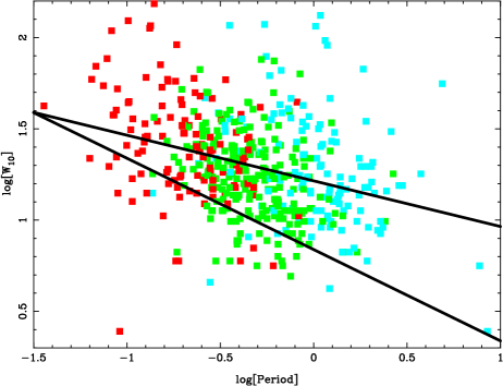
Figure 1: Profile widths at 10% of the peak value versus pulse period for 475 pulsars at an observing frequency of 1.4 GHz. Red points are pulsars with $\dot{E}>10^{34}$ erg s^-1, green points have $10^{32}$ erg s${}^{-1}<\dot{E}<10^{34}$ erg s^-1 and blue points have $\dot{E}<10^{32}$ erg s^-1. The lower-bound line, $W_{\rm 10}=6.9\degr P^{-0.5}$, used by Gould & Lyne (1998) is shown as is the fit to our data, $W_{\rm 10}=15.8\degr P^{-0.28}$.

3 Dataset and Analysis

We use the 600 pulsars observed at 1.4 GHz using the Parkes telescope and described in the paper by Johnston & Kerr (2018). This is a homogeneous sample of southern hemisphere pulsars brighter than $\sim$0.7 mJy. In that paper, only values of $W_{50}$ (the width of the profile at 50% of the peak) were listed but we have developed a method for measuring $W_{10}$ (the width of the profile at 10% of the peak) in the presence of noise, enabling us to measure accurate values for both high and low peak signal-to-noise ratio profiles.

The method relies on the assumption that the data consist of signal and a white noise term. For simplicity, it is assumed that the variance of the white noise term is constant across the profile (homoscedastic), whereas in reality, the variance will be slightly greater for parts of the profile where the signal is stronger (heteroscedastic). The signal is assumed to be a smooth function of pulse phase, and no other assumption is made. We then use the data to derive a Gaussian Process for each profile, which is a Bayesian, non-parametric model, in the sense that no assumption is made about the functional form of the pulse profile with phase (Roberts et al., 2012, GP). The GP requires prior choice of a covariance function, which governs the way in which the intensity at a given pulse phase affects and is affected by its surroundings. We use a squared exponential covariance function, as it satisfies our smoothness assumption and is infinitely differentiable, providing us with a means to analytically compute the derivatives of the model:

$$k(x_{i},x_{j})=h^{2}\exp\left[-\left(\frac{x_{i}-x_{j}}{\lambda}\right)^{2}\right],$$ (3)

where $h$ and $\lambda$ are two hyper-parameters that control the magnitude and length-scale of the covariance. The full covariance matrix of the GP is then:

$$\bf{V}(\bf{x},\bf{x})=\bf{K}(\bf{x},\bf{x})+\sigma^{2}\bf{I},$$ (4)

where $\bf{K}$ is the covariance matrix whose elements are given in Eq. 3, and $\bf{V}$ the covariance matrix including the white noise term mentioned above. In total, this model has three hyper-parameters, adding $\sigma$ to the aforementioned two. Roberts et al. (2012) explain how the hyper-parameters are best determined, and we follow their guidance in our solution. It is worth considering for a moment the potential of modeling pulse profiles in this way. First, there is no requirement for a definition of an on-pulse and off-pulse region to determine the noise variance. Secondly, the model can be separated into its two constituent parts, the signal and the noise, effectively yielding an optimized version of a noiseless profile, given the data. Thirdly, the derivatives of the signal model can be computed analytically. While it is true that the shape of pulsar profiles suggests that a model with pulse-phase dependent hyper-parameters would be more appropriate than the model we have used here, in practice, the model performs exceptionally well in produce noiseless profiles of very high fidelity.

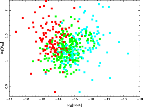
Figure 2: Period derivative ($\dot{P}$) versus $W_{10}$ for 475 pulsars. The colour convention is as per Figure 1.

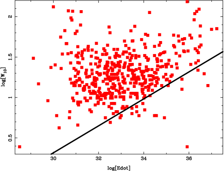
Figure 3: Spin-down energy ($\dot{E}$) versus $W_{10}$ for 475 pulsars. The straight line has a slope of $-1/6$ as expected if $W\propto P^{-0.5}$.

.

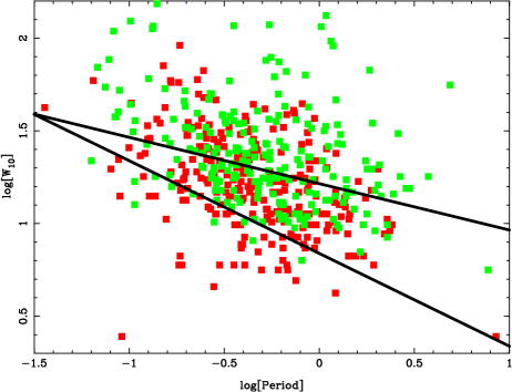
Figure 4: Profile widths at 10% of the peak value versus pulse period for 254 single pulsars (red) and 232 multiple pulsars (green).

4 Results

From the 600 pulsars in the sample, we removed 32 which showed obvious signs of scatter-broadening (Johnston & Kerr, 2018) and removed a further 4 pulsars with no measured $\dot{P}$ or $\dot{E}$. From the remaining 564 pulsars, we measured $W_{10}$ for 475 and were unable to obtain a fit for 89 pulsars with a measured peak low signal-to-noise ratio smaller than 10. Finally, for 9 pulsars showing interpulse emission we separately measured $W_{10}$ for both the main and interpulses, giving a grand total of 484 measured widths. Given that all width measurements are conducted on high signal-to-noise ratio profiles ($>10$), the error associated with the measurement is small compared to the spread in measured widths of the sample. It is indicative that the width error associated with the noisiest profiles corresponds to a few phase bins, or $\sim 1\degr$.

Figure 1 shows $W_{10}$ versus $P$ for these pulsars. There is a strong anti-correlation between the parameters and a large scatter about the mean trend. Two lines are shown in Figure 1. The first is the lower bound defined by $W_{10}=6.9\degr P^{-0.5}$ as given in Gould & Lyne (1998) and the second is a straight line fit through the data which yields $W_{10}=15.8\degr(\pm 0.6)P^{-0.28\pm 0.03}$. The lower bound in Figure 1 comes from the widespread claim in the literature that, for a constant emission height, the minimum width is given when $\alpha=90\degr$, $\beta=0\degr$ (Rankin, 1990; Gould & Lyne, 1998; Maciesiak et al., 2012). However, this is incorrect. First, higher values of $\beta$ will reduce the width and, secondly, if the polar cap is not filled and/or the beam is patchy this will also decrease the observed width.

The pulsar with the narrowest width, PSR J1028$-$5819 with a spin-period of 91 ms (Keith et al., 2008), lies more than an order of magnitude below the Gould & Lyne (1998) line. It has a double-peaked radio profile with a high degree of polarization and is a $\gamma$-ray emitter; either its radio beam is extraordinarily underfilled or the line-of-sight just cuts through the very edge of the beam. The pulsar with the widest (unscattered) profile is PSR J1015$-$5719 with a width of 153° and a spin period of 140 ms.

Figure 2 shows $W_{10}$ versus $\dot{P}$, the derivative of the spin period. There is no correlation between the parameters, with a large scatter in $W_{10}$ at all values of $\dot{P}$. Figure 3 shows $W_{10}$ versus $\dot{E}$, the rotational spin-down energy of the pulsar. As $\dot{E}\propto P^{-3}\dot{P}$ so if $W_{10}\propto P^{-1/2}$ and is uncorrelated with $\dot{P}$ then $W_{10}\propto\dot{E}^{1/6}$. Indeed, at values of $\dot{E}>10^{33}$ erg s^-1 this slope is observed in the data albeit with low significance. Below $\dot{E}\sim 10^{33}$ erg s^-1 however, the measured widths do not continue to decline and if anything, appear to increase contrary to expectations, with a significant number of pulsars with $\dot{E}<10^{32}$ erg s^-1 and $W_{10}>30\degr$, an order of magnitude larger than expectations.

Figure 5: Period-width diagram for pulsars showing emission from both poles. Squares denote the measurements with the colours representing $\dot{E}$ as in Figure 1. The underlying heat map represents the log of the pdf of a simulation which has a fixed $\alpha=85\degr$, $h_{em}$ between 200 and 400 km, and the average filling fraction set to 0.7. Contours denote 0.5, 1.0 and 1.5-$\sigma$ down from the peak of the heat map.

4.1 Single versus multiple components

We sub-divided the 600 pulsars into two main classes. The first class, the ‘singles’, shows a single, gaussian-like component with no evidence of multiple components. The second class, the ‘multiples’, shows clear evidence for multiple components in the profile. There are 254 pulsars (52%) in the first class and 232 (48%) in the second class with the rest (124 pulsars) either too weak or ambiguous to classify. Figure 4 shows the same plane as Figure 1 for pulsars in these two classes. Both classes occupy the entire period space and there is strong overlap in the widths of the two classes. However, of the 36 pulsars with $W_{10}>50\degr$, only 8 have a single component. Conversely, of the 62 pulsars with $W_{10}<10\degr$ only 12 are multiple component pulsars. On average, pulsars with multiple components are 50% wider than those with only one component; fitting a straight line through the data yields $W_{10}=12.3\degr(\pm 0.6)P^{-0.34\pm 0.04}$, and for $W_{10}=19.5\degr(\pm 0.9)P^{-0.26\pm 0.04}$ for the single and multiple component pulsars respectively.

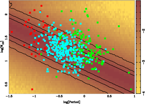
Figure 6: Period-width diagram for 475 pulsars. Squares denote the measurements with the colours representing $\dot{E}$ as in Figure 1. $\alpha$ has a random distribution for all $P$, $h_{em}$ lies between 200 and 400 km, and the average filling fraction set to 0.7. Colour coding of the background and the contours are as per Figure 5.

5 Implications and Discussion

How then do we overcome the issues outlined in Section 2.7 in order to make sense of the observed profile widths presented in Section 4?

5.1 Simulations

We create a simulation such that it is possible to obtain a probability density function (pdf) for the width of a pulsar profile given its period and a set of free parameters. The free parameters are:

• a functional form for the pdf of $h_{em}$ including a possible dependence with age or spin-down energy

• a functional form for the pdf of $s$ including a possible dependence of $s$ on $\alpha$

• a functional form for the pdf of $\alpha$ including a possible dependence with age or spin period

• a functional form for the pdf of $f$, the filling fraction of the beam

We retain the simplification of circular beams. This implies that $\beta$ can be drawn from a flat distribution between $\pm\rho$ once $\rho$ is determined. A Monte-Carlo simulation using the free parameters will then yield a probability density function for $\rho$ via Equation 1 and hence $W$ via Equation 2 for a given combination of pulsar geometry, period, age and spin-down energy.

5.2 Interpulses

The interpulse pulsars are critical to the results for two reasons. First, $\alpha\approx 90\degr$ thereby simplifying the relationship between $W$ and $\rho$ (see equation 2). Secondly, for these pulsars we often know the full geometry well (see e.g. Kramer & Johnston 2008; Keith et al. 2010) including $\beta$ and $h_{em}$. Note that $\alpha_{IP}=180\degr-\alpha_{MP}$ and $\beta_{IP}=180\degr-2\alpha_{MP}+\beta_{MP}$ so that in some instances $\beta_{MP}$ can be very different from $\beta_{IP}$ with the subsequent implications for a difference in measured width between the main and interpulse. There is also no a-priori reason why the emission height of the main and interpulses should be the same.

Generally Keith et al. (2010) find that $h_{em}<300$ km (except for PSR J1057–5552) and that the beams are somewhat underfilled. In the dataset used here, there are 19 interpulse pulsars and we can measure $W_{10}$ for 16 of the main pulses and for 10 of the interpulses. Note that, unlike in Maciesiak et al. (2011) we do not attempt to identify ‘core’ components in these pulsars but measure the full width ($W_{10}$) of the profile. Figure 5 shows the period-width plane for these 26 values. A straight line fit to these data yields $W_{10}=10.7\degr(\pm 2.1)P^{-0.21\pm 0.12}$, thus a similar slope to the data as a whole but a narrower width (as expected given that $\alpha\approx 90\degr$). If we fix the slope at $-0.5$ then the result is $W_{10}=6.8\degr(\pm 0.7)P^{-0.5}$, similar to that found by (Gould & Lyne, 1998).

We find that the simulation cannot reproduce these widths using only a spread in $h_{em}$. Rather, a combination of filling factor and heights are required for the simulation to match the data. There is also additional evidence that the narrow widths seen in e.g. PSR J1611–5209 require that the beam be underfilled (Keith et al., 2010). The data can be reproduced with a range in $h_{em}$ between 200 and 400 km and with the average filling fraction set to 0.7.

The resultant log of the pdf of the simulation is given as the background colour scale on Figure 5. The fit is acceptable, the only two outliers are the interpulse width for PSR J1057–5226 and PSR J1825–0925. For PSR J1057–5226, $\alpha$ is as low as $70\degr$ and $s$ may be larger than 1 (Weltevrede & Wright, 2009). PSR J1825–0925 which may be aligned and not an orthogonal rotator (see the arguments and counterarguments in Dyks et al. 2005 and Hermsen et al. 2017). The simulation is also able to reproduce the difference in widths between the main and interpulses; this is largely due to the differing values of $\beta$ between the two lines-of-sight, something which Maciesiak et al. (2011) do not take into account.

5.3 Extension to the whole dataset

Given the result for the interpulse pulsars, we fix the emission height range and the filling factor to those used in Figure 5. To extend these results to the entire dataset, we need an $\alpha$ distribution and we therefore assume that the intrinsic distribution is random. Because of the effects of beaming, the observed distribution is sinusoidal (i.e. it peaks at $\alpha=90\degr$). The results are shown in Figure 6.

It is immediately noticeable that although the bulk of the pulsars fall within the highest contours of the pdf, the observed distribution has a higher mean than the simulation and there are a substantial fraction of pulsars which are significantly wider observationally than expected in the simulation. Furthermore, the simulation predicts a much larger number of interpulses than seen in the observational data. These deviations mean that the assumptions going into producing the simulation are not correct; either the $\alpha$ distribution is not random, and/or there is some dependence with $s$ on $\alpha$.

Figure 7: Probability density function of $\alpha$ shown for 5 values of log($P$) in equal steps from $-1.25$ to $+0.75$.

5.4 Decay of $\alpha$ with time

If $\alpha$ decays with time (as Figures 3 and 6 seem to hint at) then older pulsars should also have larger pulse widths as a result, relative to the no decay case. Problematically we cannot determine the true age of a pulsar as the so-called characteristic age, $\tau_{c}=P/(2\dot{P})$, has been shown not to be a good indicator, especially for older pulsars as shown in JK17. This makes it hard to include $\alpha$ decay in the simulations. To achieve this, we must find a way to use $P$ as a proxy for age and therefore to establish $\alpha$ as a function of $P$. We can draw on the results of the simulation in JK17, who incorporated $\alpha$-decay and were able to match their simulated pulsar population with the observed population. This gives us the probability density function of $\alpha$ as a function of $P$ for the simulated pulsars that also pass the detection criteria.

To assess what happens if we include $\alpha$ decay in this way into the current simulation, we convolve the original random distribution in $\alpha$ with a cut-off which depends on $P^{2}$. The resultant probability density function of $\alpha$ for 5 different spin periods is shown in Figure 7. These distributions are consistent with those found for pulsars with different pulse periods in the work of JK17. Including this form of $\alpha$-decay in the simulations here leads to the results shown in Figure 8. The main difference between Figures 8 and 6 is that the pdf bends upwards at large $P$ as the $\alpha$ distribution is skewed towards smaller values at these periods.

We assess the requirement to include $\alpha$ decay in the following way. First we compute the peak of the simulated pulse-width distribution for each $P$ in the range we have simulated, i.e. the most likely pulse width for each period. We subtract the pulse widths for both the simulation and the observed distribution from this peak value. This has the effect of removing the correlation between $W$ and $P$ allowing us to compare the distribution across period. We bin the data into 3 bins across the period axis, $P<0.3$ s, $0.3<P<1.0$ s, $P>1.0$ s. Figure 9 shows the histograms of the resulting distributions for the simulation and the observations for the cases without and with $\alpha$-decay. Clearly, without $\alpha$-decay, the match between the histograms is poor especially for pulsars with long periods, whereas with $\alpha$-decay the simulation and data match well in all 3 period bins.

5.5 Dependence of $s$ on $\alpha$

It is already well established that high $\dot{E}$ pulsars have wide profiles (Johnston & Weisberg, 2006) and these could be caused by high emission heights (Karastergiou & Johnston, 2007; Weltevrede & Johnston, 2008a) or emission from outside the conventional polar cap region (Rookyard et al., 2015b). Rookyard et al. (2015b) have derived a dependence for $s$ on $\alpha$ via the equation

$$s=-0.022\alpha+2.80$$ (5)

with $\alpha$ in degrees. We note that this maintains $s\sim 1$ when $\alpha\sim 90\degr$ and so this does not change the results for the interpulses given in Figure 5. However, for low values of $\alpha$ it allows $s$ to be significantly larger than 1 which results in a larger distribution of possible widths. At the same time, Rookyard et al. (2015b) recognised that the filling factor of the beams was small and that many components were “missing” which meant that the ‘true’ widths they assumed were significantly larger than the observed widths. It is not clear how the results from their sample of high $\dot{E}$ gamma-ray pulsars can be extrapolated to the long-period, low $\dot{E}$ bulk of the pulsar population. We do not include this effect in our simulations.

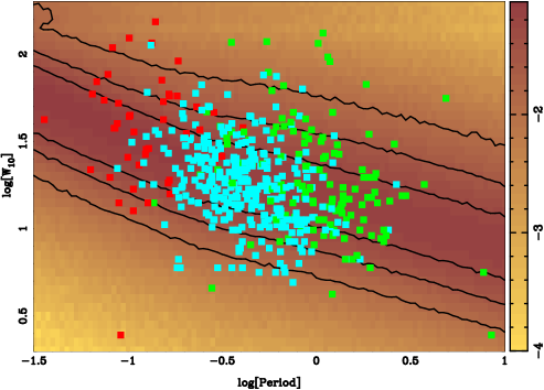
Figure 8: As for Figure 6 with the addition of an $\alpha$ distribution which depends on $P$ (see text and Figure 7 for details). Squares denote the measurements with the colours representing $\dot{E}$ as in Figure 1. Colour coding of the background and the contours are as per Figure 5.

Figure 9: Histogram of the difference between the simulated (or observed) pulse width versus the expected pulse width for different values of $P$. Bottom panels: Results from the case without $\alpha$-decay see Figure 6. Top panels: Results from the case with $\alpha$-decay; see Figure 8. From left to right, panels represent pulsars with $P<0.3$ s, $0.3<P<1.0$ s, $P>1.0$ s, the solid line represents the simulation and the dashed line the observed population.

5.6 Singles and multiples

What are the implications of the relative fraction of singles and multiples and the differences between the widths of single and multipe component pulsars?

In a simple version of the Rankin beam models, the numbers can be reconciled if the core component is relatively large and the the conal component occupies a large fraction of the beam. In this case, a large fraction of single components can be obtained by cutting through the cone at moderate to high $\beta$ and these single components will also be relatively wide compared to double components at lower $\beta$. In addition, narrow single components can be obtained where the cone is not present and the line of sight cuts through the core component.

In the patchy model of Lyne & Manchester (1988), the number of active patches along the line of sight determines the profile shape. In order to have an equal fraction of single and multiple profile pulsars, the patch size must be relatively large and should overlap frequently. This seems consistent with the mean beam emissivity shown by Han & Manchester (2001).

6 Summary

We have used the database of pulsars provided by Johnston & Kerr (2018) and a novel method based on a Gaussian Process technique to determine the pulse widths at the 10% level for a sample of 600 pulsars at an observing frequency of 1.4 GHz. We have investigated the relationship between a pulsar’s spin period and its width and find that:

• for a given spin period, a broad range of widths are observed, although the general trend is that $W_{10}\propto P^{-0.3}$.

• emission heights are low and have a narrow range between 200 and 400 km irrespective of $P$.

• pulsars which have interpulse emission and are orthogonal rotators show evidence for an underfilled beam; i.e. their pulse widths are narrower than expected.

• pulsars with low $\dot{E}$ have wider profiles than expected from their spin periods; this is most likely due to $\alpha$ decay in this older population.

• there should exist a population of long-period, low-$\alpha$ pulsars which are difficult to detect with standard techniques but which may be amenable to discover via a fast-folding algorithm (Cameron et al., 2017).

• pulsars with multiple components are wider than those with only one component. This has implications for the overall beam structure and the size of the emitting regions, but it remains difficult to distinguish between the models of Rankin (1993) and Lyne & Manchester (1988).

References

- Blaskiewicz et al. (1991) Blaskiewicz M., Cordes J. M., Wasserman I., 1991, ApJ, 370, 643
- Cameron et al. (2017) Cameron A. D., Barr E. D., Champion D. J., Kramer M., Zhu W. W., 2017, MNRAS, 468, 1994
- Clifton & Weisberg (2008) Clifton T., Weisberg J. M., 2008, ApJ, 679, 687
- Desvignes et al. (2013) Desvignes G., Kramer M., Cognard I., Kasian L., van Leeuwen J., Stairs I., Theureau G., 2013, in IAU Symposium, Vol. 291, van Leeuwen J., ed, Neutron Stars and Pulsars: Challenges and Opportunities after 80 years, p. 199
- Dyks et al. (2005) Dyks J., Zhang B., Gil J., 2005, ApJ, 626, L45
- Fonseca et al. (2014) Fonseca E., Stairs I. H., Thorsett S. E., 2014, ApJ, 787, 82
- Gangadhara (2004) Gangadhara R. T., 2004, ApJ, 609, 335
- Gil et al. (1984) Gil J., Gronkowski P., Rudnicki W., 1984, A&A, 132, 312
- Gil et al. (1993) Gil J. A., Kijak J., Seiradakis J. H., 1993, A&A, 272, 268
- Gould & Lyne (1998) Gould D. M., Lyne A. G., 1998, MNRAS, 301, 235
- Gupta & Gangadhara (2003) Gupta Y., Gangadhara R. T., 2003, ApJ, 584, 418
- Han & Manchester (2001) Han J. L., Manchester R. N., 2001, MNRAS, 320, L35
- Hermsen et al. (2017) Hermsen W. et al., 2017, MNRAS, 466, 1688
- Johnston & Karastergiou (2017) Johnston S., Karastergiou A., 2017, MNRAS, 467, 3493
- Johnston & Kerr (2018) Johnston S., Kerr M., 2018, MNRAS, 474, 4629
- Johnston & Weisberg (2006) Johnston S., Weisberg J. M., 2006, MNRAS, 368, 1856
- Karastergiou & Johnston (2007) Karastergiou A., Johnston S., 2007, MNRAS, 380, 1678
- Keith et al. (2008) Keith M. J., Johnston S., Kramer M., Weltevrede P., Watters K. P., Stappers B. W., 2008, MNRAS, 389, 1881
- Keith et al. (2010) Keith M. J., Johnston S., Weltevrede P., Kramer M., 2010, MNRAS, 402, 745
- Kramer & Johnston (2008) Kramer M., Johnston S., 2008, MNRAS, 390, 87
- Kramer et al. (1994) Kramer M., Wielebinski R., Jessner A., Gil J. A., Seiradakis J. H., 1994, A&AS, 107
- Kramer et al. (1998) Kramer M., Xilouris K. M., Lorimer D. R., Doroshenko O., Jessner A., Wielebinski R., Wolszczan A., Camilo F., 1998, ApJ, 501, 270
- Lazarus et al. (2015) Lazarus P. et al., 2015, ApJ, 812, 81
- Lyne et al. (2013) Lyne A., Graham-Smith F., Weltevrede P., Jordan C., Stappers B., Bassa C., Kramer M., 2013, Science, 342, 598
- Lyne & Manchester (1988) Lyne A. G., Manchester R. N., 1988, MNRAS, 234, 477
- Maciesiak & Gil (2011) Maciesiak K., Gil J., 2011, MNRAS, 417, 1444
- Maciesiak et al. (2012) Maciesiak K., Gil J., Melikidze G., 2012, MNRAS, 424, 1762
- Maciesiak et al. (2011) Maciesiak K., Gil J., Ribeiro V. A. R. M., 2011, MNRAS, 414, 1314
- Manchester et al. (2010) Manchester R. N. et al., 2010, ApJ, 710, 1694
- McKinnon (1993) McKinnon M. M., 1993, ApJ, 413, 317
- Mitra & Rankin (2002) Mitra D., Rankin J. M., 2002, ApJ, 577, 322
- Mitra & Rankin (2011) Mitra D., Rankin J. M., 2011, ApJ, 727, 92
- Narayan & Vivekanand (1983) Narayan R., Vivekanand M., 1983, A&A, 122, 45
- Rankin (1990) Rankin J. M., 1990, ApJ, 352, 247
- Rankin (1993) Rankin J. M., 1993, ApJ, 405, 285
- Ravi et al. (2010) Ravi V., Manchester R. N., Hobbs G., 2010, ApJ, 716, L85
- Roberts et al. (2012) Roberts S., Osborne M., Ebden M., Reece S., Gibson N., Aigrain S., 2012, Philosophical Transactions of the Royal Society of London Series A, 371, 20110550
- Rookyard et al. (2015a) Rookyard S. C., Weltevrede P., Johnston S., 2015a, MNRAS, 446, 3367
- Rookyard et al. (2015b) Rookyard S. C., Weltevrede P., Johnston S., 2015b, MNRAS, 446, 3356
- Ruderman & Sutherland (1975) Ruderman M. A., Sutherland P. G., 1975, ApJ, 196, 51
- Skrzypczak et al. (2018) Skrzypczak A., Basu R., Mitra D., Melikidze G. I., Maciesiak K., Koralewska O., Filothodoros A., 2018, ApJ, 854, 162
- Szary & van Leeuwen (2017) Szary A., van Leeuwen J., 2017, ApJ, 845, 95
- Tauris & Manchester (1998) Tauris T. M., Manchester R. N., 1998, MNRAS, 298, 625
- van Heerden et al. (2017) van Heerden E., Karastergiou A., Roberts S. J., 2017, MNRAS, 467, 1661
- Wang et al. (2014) Wang H. G. et al., 2014, ApJ, 789, 73
- Weltevrede & Johnston (2008a) Weltevrede P., Johnston S., 2008a, MNRAS, 391, 1210
- Weltevrede & Johnston (2008b) Weltevrede P., Johnston S., 2008b, MNRAS, 387, 1755
- Weltevrede & Wright (2009) Weltevrede P., Wright G., 2009, MNRAS, 395, 2117
- Wright & Weltevrede (2017) Wright G., Weltevrede P., 2017, MNRAS, 464, 2597
- Young et al. (2010) Young M. D. T., Chan L. S., Burman R. R., Blair D. G., 2010, MNRAS, 402, 1317