Learning Deep Stochastic Optimal Control Policies using Forward-Backward SDEs

Abstract

In this paper we propose a new methodology for decision-making under uncertainty using recent advancements in the areas of nonlinear stochastic optimal control theory, applied mathematics, and machine learning. Grounded on the fundamental relation between certain nonlinear partial differential equations and forward-backward stochastic differential equations, we develop a control framework that is scalable and applicable to general classes of stochastic systems and decision-making problem formulations in robotics and autonomy. The proposed deep neural network architectures for stochastic control consist of recurrent and fully connected layers. The performance and scalability of the aforementioned algorithm are investigated in three non-linear systems in simulation with and without control constraints. We conclude with a discussion on future directions and their implications to robotics.

I Introduction

Over the past 15 years there has been significant interest from the robotics community in developing algorithms for stochastic control of systems operating in dynamic and uncertain environments. This interest was initiated by two main developments related to theory and hardware. From a theoretical standpoint, there has been a better – and in some sense deeper – understanding of connections between different disciplines. As an example, the connections between optimality principles in control theory and information theoretic concepts in statistical physics are well understood so far [1, 2, 3, 4]. These connections have resulted in novel algorithms that are scalable, real-time, and can handle complex nonlinear dynamics [5]. On the hardware side, there have been significant technological developments that made possible the use of high performance computing for real-time Stochastic Optimal Control (SOC) in robotics [6].

Traditionally, SOC problems are solved using Dynamic Programming (DP). Dynamic Programming requires solving a nonlinear second order Partial Differential Equation (PDE) known as the Hamilton-Jacobi-Bellman (HJB) equation [7]. It is well-known that the HJB equation suffers from the curse of dimensionality. One way to tackle this problem is through an exponential transformation to linearize the HJB equation, which can then be solved with forward sampling using the linear Feynman-Kac lemma [8] [9]. While the linear Feynman-Kac lemma provides a probabilistic representation of the solution to the HJB that is exact, its application relies on certain assumptions between control authority and noise. In addition, the exponential transformation of the value function reduces the discriminability between good and bad states, which makes the computation of the optimal control policy difficult.

An alternative approach to solve SOC problems is to transform the HJB into a system of Forward-Backward Stochastic Differential Equations using a nonlinear version of the Feynman-Kac lemma [10, 11]. This is a more general approach compared to the standard Path Integral control framework, in that it does not rely on any assumptions between control authority and noise. In addition, it is valid for general classes of stochastic processes including jump-diffusions and infinite dimensional stochastic processes [12, 13]. However, the main challenge in using the nonlinear Feynman-Kac lemma lies in the solution of the backward SDE. This process requires the back-propagation of a conditional expectation, and thus cannot be solved by simple trajectory integration, as it is done with forward SDEs. Therefore, numerical approximation techniques are needed for utilization in an actual algorithm. Exarchos and Theodorou [14] developed an importance sampling based iterative scheme by approximating the conditional expectation at every time step using linear regression (see also [15] and [16]). However, this method suffers from compounding errors from Least Squares approximation at every time step.

Recently, the idea of using Deep Neural Networks and other data-driven techniques for approximating the solutions of non-linear PDEs has been garnering significant attention. In Raissi et al. [17], DNNs were used for both solving and data-driven discovery of the coefficients of non-linear PDEs popular in physics literature such as the Schrödinger, the Allen-Cahn, the Navier-Stokes, and the Burgers equations. They have demonstrated that their DNN-based approach can surpass the performance of other data-driven methods such as sparse linear regression proposed by Rudy et al. [18]. On the other hand, using DNNs for end-to-end Model Predictive Optimal Control (MPOC) has also become a popular research area. Pereira et al. [19] introduced a DNN architecture for Imitation Learning (IL), inspired by MPOC, based on the Path Integral (PI) Control approach alongside Amos et al. [20] who introduced an end-to-end MPOC architecture that uses the KKT conditions of the convex approximation. Pan et al. [21] demonstrated the MPOC capabilities of a DNN control policy using only camera and wheel speed sensors, through IL. Morton et al. [22] used a Koopman operator based DNN model for learning the dynamics of fluids and performing MPOC for suppressing vortex shedding in the wake of a cylinder.

This tremendous success of DNNs as universal function approximators [23] inspires an alternative scheme to solve systems of FBSDEs. Recently, Han et al. [24] introduced a Deep Learning based algorithm to solve FBSDEs associated with nonlinear parabolic PDEs. Their framework was applied to solve the HJB equation for a white-noise driven linear system to obtain the value function at the initial time step. This framework, although effective for solving parabolic PDEs, can not be applied directly to solve the HJB for optimal control of unstable nonlinear systems since it lacks sufficient exploration and is limited to only states that can be reached by purely noise driven dynamics. This problem was addressed in [14] through application of Girsanov’s theorem, which allows for the modification of the drift terms in the FBSDE system thereby facilitating efficient exploration through controlled forward dynamics.

In this paper, we propose a novel framework for solving SOC problems of nonlinear systems in robotics. The resulting algorithms overcome limitations of previous work in [24] by exploiting Girsanov’s theorem as in [14] to enable efficient exploration and by utilizing the benefits of recurrent neural networks in learning temporal dependencies. We begin by proposing essential modifications to the existing framework of FBSDEs to utilize the solutions of the HJB equation at every timestep to compute an optimal feedback control which thereby drives the exploration to optimal areas of the state space. Additionally, we propose a novel architecture that utilizes Long-Short Term Memory (LSTM) networks to capture the underlying temporal dependency of the problem. In contrast to the individual Fully Connected (FC) networks in [24], our proposed architecture uses fewer parameters, is faster to train, scales to longer time horizons and produces smoother control trajectories. We also extend our framework to problems with control-constraints which are very relevant to most applications in Robotics wherein actuation torques must not violate specified box constraints. Finally, we compare the performance of both network architectures on systems with nonlinear dynamics such as pendulum, cartpole and quadcopter in simulation.

The rest of this paper is organized as follows: in Section II we reformulate the stochastic optimal control problem in the context of FBSDE. In Section III we use the same FBSDE framework to the control constrained case. Then we provide the Deep FBSDE Control algorithm in Section IV. The simulation results are included in Section V. Finally we conclude the paper and discuss future research directions.

II Stochastic Optimal Control through FBSDE

II-A Problem Formulation

Let ($\Omega,\mathcal{F},\{\mathcal{F}_{t}\}_{t\geq 0},\mathbb{Q}$) be a complete, filtered probability space on which a $v$-dimensional standard Brownian motion $w(t)$ is defined, such that $\{\mathcal{F}_{t}\}_{t\geq 0}$ is the normal filtration of $w(t)$. Consider a general stochastic nonlinear system with control affine dynamics,

$$\mathrm{d}x(t)=f(x(t),t)\mathrm{d}t+G(x(t),t)u(x(t),t)\mathrm{d}t+\Sigma(x(t),t)\mathrm{d}w(t)$$ (1)

where, $0<t<T<\infty$, $T$ is the time horizon, $x\in\mathbb{R}^{n}$ is the state vector, $u\in\mathbb{R}^{m}$ is the control vector, $f:\mathbb{R}^{n}\times[0,T]\rightarrow\mathbb{R}^{n}$ represents the drift, $G:\mathbb{R}^{n}\times[0,T]\rightarrow\mathbb{R}^{n\times m}$ represents the actuator dynamics, $\Sigma:\mathbb{R}^{n}\times[0,T]\rightarrow\mathbb{R}^{n\times v}$ represents the diffusion. The Stochastic Optimal Control problem can be formulated as minimization of an expected cost functional given by

$$J\big{(}x(t),t\big{)}=\mathbb{E}_{\mathbb{Q}}\Big{[}g\big{(}x(T)\big{)}+\int_{t}^{T}\big{(}q(x(\tau)\big{)}+\frac{1}{2}u^{\mathrm{T}}Ru)\mathrm{d}\tau\Big{]},$$ (2)

where $g:\mathbb{R}^{n}\rightarrow\mathbb{R}^{+}$ is the terminal state cost, $q:\mathbb{R}^{n}\rightarrow\mathbb{R}^{+}$ is the running state cost and $R$ is a $m\times m$ positive definite matrix. The expectation is taken with respect to the probability measure $\mathbb{Q}$ over the space of trajectories induced by controlled stochastic dynamics. With the set of all admissible controls $\mathcal{U}$, we can define the value function as,

$$\begin{cases}V\big{(}x(t),t\big{)}&=\inf_{u(.)\in\mathcal{U}[0,T]}J\big{(}x(t),t\big{)}\\ V\big{(}x(T),T\big{)}&=g\big{(}x(T)\big{)}.\end{cases}$$ (3)

Using stochastic Bellman’s principle, as shown in [10], if the value function is in $C^{1,2}$, then its solution can be found with Ito’s differentiation rule to satisfy the Hamilton-Jacobi-Bellman equation,

$$\begin{cases}V_{t}+\inf_{u(\cdot)\in\mathcal{U}[0,T]}\Big{\{}\frac{1}{2}\operatorname{\rm{tr}}(V_{xx}\Sigma\Sigma^{\mathrm{T}})+V_{x}^{\mathrm{T}}(f+Gu)+q\\ +\frac{1}{2}u^{\mathrm{T}}Ru\Big{\}}=0\\ V(x(T),T)=g(x(T)),\end{cases}$$ (4)

where $V_{x},V_{xx}$ denote the gradient and Hessian of $V$ respectively. The explicit dependence on independent variables in the PDE above and all PDEs henceforth is omitted for the sake of conciseness, but will be maintained for their corresponding SDEs for clarity. For the chosen form of the cost functional integrand, the infimum operation can be carried out by taking the gradient of the terms inside, known as the Hamiltonian, with respect to $u$ and setting it to zero,

$$G^{\mathrm{T}}(x(t),t)V_{x}(x(t),t)+Ru(x(t),t)=0.$$ (5)

Therefore, the optimal control is obtained as

$$u^{*}(x(t),t)=-R^{-1}G^{\mathrm{T}}(x(t),t)V_{x}(x(t),t).$$ (6)

Plugging the optimal control back into the original HJB equation, the following form of the equation is obtained,

$$\begin{cases}V_{t}+\frac{1}{2}\operatorname{\rm{tr}}(V_{xx}\Sigma\Sigma^{\mathrm{T}})+V_{x}^{\mathrm{T}}f+q-\frac{1}{2}V_{x}^{\mathrm{T}}GR^{-1}G^{\mathrm{T}}V_{x}=0\\ V(x(T),T)=g(x(T)).\end{cases}$$ (7)

II-B Non-linear Feynman-Kac lemma

Here we restate the non-linear Feynman-Kac lemma from [14]. Consider the Cauchy problem,

$$\begin{cases}\nu_{t}+\frac{1}{2}\operatorname{\rm{tr}}\big{(}\nu_{xx}\Sigma\Sigma^{\mathrm{T}}\big{)}+\nu_{x}^{\mathrm{T}}b+h=0\\ \nu(x(T),T)=g(x(T)),\,x\in\mathbb{R}^{n},\end{cases}$$ (8)

wherein the functions $\Sigma(x(t),t)$, $b(x(t),t)$, $h(x,\nu,z,t)$ and $g(x(T))$ satisfy mild regularity conditions [14]. Then, (8) admits a unique (viscosity) solution $\nu:\mathbb{R}^{n}\times[0,T]\rightarrow\mathbb{R}$, which has the following probabilistic representation,

$$\nu(x(t),t) =y(t)$$ (9)

$$\Sigma^{\mathrm{T}}\nu_{x}(x(t),t) =z(t)$$ (10)

wherein $\big{(}x(\cdot),y(\cdot),z(\cdot)\big{)}$ is the unique solution of an FBSDE system. The forward component of that system is given by

$$\begin{cases}\mathrm{d}x(t)&=b(x(t),t)\mathrm{d}t+\Sigma(x(t),t)\mathrm{d}w(t)\\ x(0)&=\xi\\ \end{cases}$$ (11)

where, without loss of generality, $w$ is chosen as a n-dimensional Brownian motion. The process $x(t)$, satisfying the above forward SDE, is also called the state process. The associated backward SDE is

$$\begin{cases}\mathrm{d}y(t)&=-h(x(t),y(t),z(t),t)\mathrm{d}t+z(t)^{\mathrm{T}}\mathrm{d}w(t)\\ y(T)&=g(x(T)).\end{cases}$$ (12)

The function $h(\cdot)$ is called the generator or driver.

We assume that there exists a matrix-valued function $\Gamma:\mathbb{R}^{n}\times[0,T]\rightarrow\mathbb{R}^{n\times m}$ such that the controls matrix $G(x(t),t)$ in (1) can be decomposed as $G(x(t),t)=\Sigma(x(t),t)\Gamma(x(t),t)$ for all $(x,t)\in\mathbb{R}^{n}\times[0,T]$, satisfying the same mild regularity conditions. This decomposition can be justified as the case of stochastic actuators, where noise enters the system through the control channels. Under this assumption, we can apply the nonlinear Feynman-Kac lemma to the HJB PDE (7) and establish equivalence to (8) with coefficients of (8) given by

$$\begin{split}b(x(t),t)&=f(x(t),t)\\ h(x(t),y(t),z(t),t)&=q(x(t))-\frac{1}{2}z^{\mathrm{T}}\Gamma R^{-1}\Gamma^{\mathrm{T}}z.\end{split}$$ (13)

II-C Importance Sampling for Efficient Exploration

There are several cases of systems in which the goal state practically cannot be reached by the uncontrolled stochastic system dynamics. This issue can be eliminated if one is given the ability to modify the drift term of the forward SDE. Specifically, by changing the drift, we can direct the exploration of the state space towards the given goal state, or any other state of interest, reachable by control. Through Girsanov’s theorem [25] on change of measure, the drift term in the forward SDE (11) can be changed if the backward SDE (12) is compensated accordingly. This is known as the importance sampling for FBSDEs. This results in a new system of FBSDEs in certain sense equivalent to the original ones,

$$\begin{cases}\mathrm{d}\tilde{x}(t)=[b(\tilde{x}(t),t)+\Sigma(\tilde{x}(t),t)K(t)]\mathrm{d}t+\Sigma(\tilde{x}(t),t)\mathrm{d}\tilde{w}(t)\\ \tilde{x}(0)=\xi,\end{cases}$$ (14)

along with the compensated BSDE,

$$\begin{cases}\mathrm{d}\tilde{y}(t)=(-h(\tilde{x}(t),\tilde{y}(t),\tilde{z}(t),t)+\tilde{z}(t)^{\mathrm{T}}K(t))\mathrm{d}t\\ +\tilde{z}(t)^{\mathrm{T}}\mathrm{d}\tilde{w}(t)\\ \tilde{y}(T)=g(\tilde{x}(T)),\end{cases}$$ (15)

for any measurable, bounded and adapted process $K:[0,T]\rightarrow\mathbb{R}^{n}$. We refer the readers to proof of Theorem 1 in [14] for the full derivation of change of measure for FBSDEs. The PDE associated with this new system is given by

$$\begin{cases}V_{t}+\frac{1}{2}\operatorname{\rm{tr}}\big{(}V_{\tilde{x}\tilde{x}}\,\Sigma\Sigma^{\mathrm{T}}\big{)}+V_{x}^{\mathrm{T}}\big{(}b+\Sigma K\big{)}+h-\tilde{z}^{\mathrm{T}}K=0\\ V(\tilde{x},T)=g(\tilde{x}(T)),\end{cases}$$ (16)

which is identical to the original problem (8) as we have merely added and subtracted the term $\tilde{z}^{\mathrm{T}}K$. Recalling the decomposition of control matrix in the case of stochastic actuators, the modified drift term can be applied with any nominal control $\bar{u}$ to achieve the controlled dynamics,

$$\begin{split}\mathrm{d}\tilde{x}(t)=\big{[}f(\tilde{x}(t),t)+\Sigma\big{(}\tilde{x}(t),t\big{)}&\Gamma\big{(}\tilde{x}(t),t\big{)}\bar{u}(t)\big{]}\mathrm{d}t\\ &+\Sigma\big{(}\tilde{x}(t),t\big{)}\mathrm{d}\tilde{w}(t)\end{split}$$ (17)

with $K(t)=\Gamma(\tilde{x}(t),t)\,\bar{u}$. The nominal control $\bar{u}$ can be any open or closed-loop control, a random control, or a control calculated from a previous run of the algorithm.

II-D FBSDE Reformulation

Solutions to BSDEs need to satisfy a terminal condition, and thus, integration needs to be performed backwards in time, yet the filtration still evolves forward in time. It turns out that a terminal value problem involving BSDEs admits an adapted solution if one back-propagates the conditional expectation of the process. This was the basis of the approximation scheme and corresponding algorithm introduced in [14]. However, this scheme is prone to approximation errors introduced by least squares estimates which compound over time steps. On the other hand, the Deep Learning (DL)-based approach in [24] uses the terminal condition of the BSDE as a prediction target for a self-supervised learning problem with the goal of using back-propagation to estimate the value function at the initial timestep. This was achieved by treating the value at the initial timestep, $V(\tilde{x}(0),0)$, as one of the trainable parameters of a DL model. There is a two-fold advantage of this approach: (i) starting with a random guess of $V(\tilde{x}(0),0;\phi)$, the backward SDE can be forward propagated instead. This eliminates the need to back-propagate a least-squares estimate of the conditional expectation to solve the BSDE and instead treat the BSDE similar to the FSDE, and (ii) the approximation errors at every time step are compensated by the backpropagation training process of DL. This is because the individual networks, at every timestep, contribute to a common goal of predicting the target terminal condition and are jointly trained.

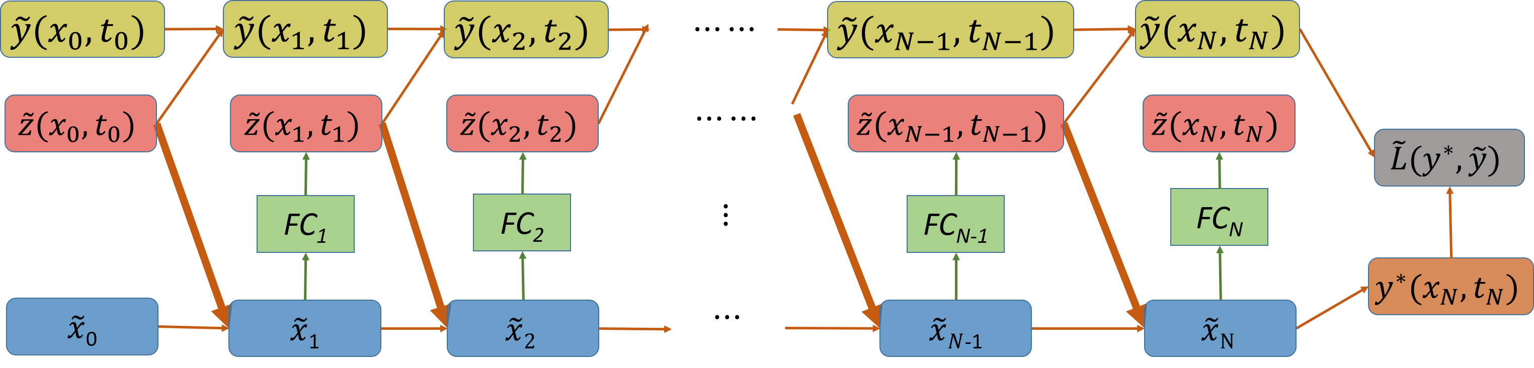
Figure 1: FC neural network architecture (boldfaced connections indicate importance sampling).

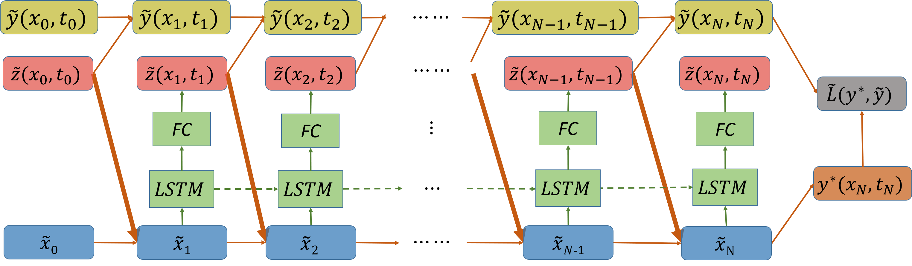
Figure 2: LSTM neural network architecture (boldfaced connections indicate importance sampling). Note that the $FC_{t}$ networks in (Fig. 1) above are different for each time step, whereas here the same weights are shared for every time step.

In this work, we combine the importance sampling concepts for FBSDEs with the Deep Learning techniques that allows for the forward sampling of the BSDE and propose a new algorithm for Stochastic Optimal Control problems. The novelty of our approach is to incorporate importance sampling for efficient exploration in the DL model. Instead of the original HJB equation (7), we focus on obtaining solutions for the modified HJB PDE in (16) by using the modified FBSDE system (14), (15). Additionally, we explicitly compute the control at every time step using the analytical expression for optimal control (6) in the computational graph. Similar to [24], the FBSDE system is solved by integration of both the SDEs forward in time as follows,

$$\begin{cases}\mathrm{d}\tilde{x}(t)=f(\tilde{x}(t),t)\mathrm{d}t+\Sigma(\tilde{x}(t),t)\big{[}\bar{u}(\tilde{x}(t),t)\mathrm{d}t+\mathrm{d}\tilde{w}(t)\big{]}\\ \bar{u}(\tilde{x}(t),t)=\Gamma u^{*}(\tilde{x}(t),t;\theta_{t})=-\Gamma R^{-1}\Gamma^{\mathrm{T}}\tilde{z}(t;\theta_{t})\\ \tilde{x}(0)=\xi\end{cases}$$ (18)

and

$$\begin{cases}\mathrm{d}\tilde{y}(t)=\big{(}-h(\tilde{x}(t),\tilde{y}(t),\tilde{z}(t;\theta_{t}),t)\\ +\tilde{z}(t;\theta_{t})^{\mathrm{T}}\,\Gamma(\tilde{x}(t),t)\,\bar{u}\big{)}\mathrm{d}t+\tilde{z}(t;\theta_{t})^{\mathrm{T}}\mathrm{d}\tilde{w}(t)\\ \tilde{y}(0)=V(\tilde{x}(0),0;\phi).\end{cases}$$ (19)

III Stochastic Control Problems with Control Constraints

The framework we have considered so far can be suitably modified to accommodate a certain type of control constraints, namely upper and lower bounds $(-u^{\max},u^{\max})$. Specifically, each control dimension component satisfies $|u_{j}(\tilde{x}(t),t)|\leq u^{\max}_{j}$ for all $j=\{1,\cdots,m\}$. Such control constraints are common in mechanical systems, where control forces and/or torques are bounded, and may be readily introduced in our framework via the addition of a “soft” constraint, integrated within the cost functional. In recent work, Exarchos et al. [26] showed how box-type control constraints for $L^{1}$-optimal control problems (also called minimum fuel problems), can be incorporated into an FBSDE scheme. These are in contrast to the more frequently used quadratic control cost ($L^{2}$ or minimum energy) SOC problems. Indeed, one can replace the cost functional given by (2) with .

$$J\big{(}\tilde{x}(t),t\big{)}=\mathbb{E}_{\mathbb{Q}}\bigg{[}g(\tilde{x}(T))+\int_{t}^{T}\bigg{(}q(\tilde{x}(t))+\sum_{j=1}^{m}S_{j}(u_{j})\bigg{)}\mathrm{d}t\bigg{]},$$ (20)

where

$$S_{j}(u_{j})=c_{j}\int_{0}^{u_{j}}\operatorname{sig}^{-1}\big{(}\frac{\mathrm{v}}{u^{\max}_{j}}\big{)}\mathrm{d}\mathrm{v},\qquad j=\{1,\ldots,m\},$$ (21)

$c_{j}$ are constant weights, $\operatorname{sig}(\cdot)$ denotes the sigmoid (tanh-like) function that saturates at infinity, i.e., $\operatorname{sig}(\pm\infty)=\pm 1$, while $\mathrm{v}$ is a dummy variable of integration. A suitable example along with its inverse is

$$\operatorname{sig}(\mathrm{v})=\frac{2}{1+e^{-\mathrm{v}}}-1,\quad\mathrm{v}\in\mathbb{R}$$ (22)

$$\operatorname{sig}^{-1}(\mathrm{\mu})=\log\bigg{(}\frac{1+\mathrm{\mu}}{1-\mathrm{\mu}}\bigg{)},\quad\mathrm{\mu}\in(-1,1).$$ (23)

Following the same procedure as in Section II, we set the derivative of the Hamiltonian equal to zero and obtain

$$-\begin{bmatrix}c_{1}\operatorname{sig}^{-1}(\frac{u_{1}}{u^{\max}_{1}})\\ \vdots\\ c_{m}\operatorname{sig}^{-1}(\frac{u_{m}}{u^{\max}_{m}})\end{bmatrix}-G^{\mathrm{T}}(\tilde{x}(t),t)v_{\tilde{x}}(\tilde{x}(t),t)=0.$$ (24)

By introducing the notation

$$G(\tilde{x}(t),t)=[\mathrm{g}_{1}(\tilde{x}(t),t)\quad\mathrm{g}_{2}(\tilde{x}(t),t)\quad\cdots\quad\mathrm{g}_{m}(\tilde{x}(t),t)]$$

where $\mathrm{g}_{i}$ (not to be confused with the terminal cost $g$) denotes the i-th column of $G$, we may write the optimal control in component-wise notation as

$$\begin{split}&u_{j}^{*}(\tilde{x}(t),t)=u^{\max}_{j}\operatorname{sig}\bigg{(}-\frac{1}{c_{j}}\mathrm{g}_{j}^{\mathrm{T}}(\tilde{x}(t),t)V_{\tilde{x}}(\tilde{x}(t),t)\bigg{)},\\ &j=\{1,\cdots,m\}\end{split}$$ (25)

The optimal control can be written equivalently in vector form. Indeed, if $[u^{\max}_{1},\ldots,u^{\max}_{m}]^{\mathrm{T}}$ is the vector of bounds, $R^{-1}=[1/c_{1},\ldots,1/c_{m}]$ is a diagonal matrix of the reciprocals of the weights and $\mathrm{U}_{max}=diag([u^{\max}_{1},\ldots,u^{\max}_{m}]^{\mathrm{T}})$ is a diagonal matrix of the bounds, one readily obtains

$$\begin{split}&u^{*}(\tilde{x}(t),t)=\mathrm{U}_{max}\operatorname{sig}\bigg{(}-R^{-1}G^{{}^{\mathrm{T}}}(\tilde{x}(t),t)V_{\tilde{x}}(\tilde{x}(t),t)\bigg{)}\end{split}$$ (26)

Substituting the equation of the constrained controls into eqn. 16 results in

$$\begin{cases}V_{t}+\frac{1}{2}\operatorname{\rm{tr}}\big{(}V_{\tilde{x}\tilde{x}}\,\Sigma\Sigma^{\mathrm{T}}\big{)}+V_{\tilde{x}}^{\mathrm{T}}\big{(}b+\Sigma K\big{)}+h-\tilde{z}^{\mathrm{T}}K=0\\ V(\tilde{x}(T),T)=g(\tilde{x}(T))\end{cases}$$ (27)

where $h$ is specified by the expression that follows:

$$h=q(\tilde{x}(t))+V_{\tilde{x}}^{\mathrm{T}}G(\tilde{x}(t),t)u^{*}(\tilde{x}(t),t)+\sum_{j=1}^{m}S_{j}(u_{j}^{*})$$ (28)

1  Given:

2$\tilde{x}_{0}=\xi,\;f,\;G$, $\Sigma,\;\Gamma$: Initial state and system dynamics;

3$g,\;q,\;R$: Cost function parameters;

4$N$: Task horizon, $K$: Number of iterations, $M$: Batch

5size; bool: Boolean for constrained control case;

6$U_{max}$: maximum controls per input channel;

$\Delta t$: Time discretization; $\lambda$: weight-decay parameter;

7  Parameters:

8$\tilde{y}_{0}=V(\tilde{x}_{0},0;\phi)$: Value function at $t=0$;

9$\tilde{z}_{0}=\Sigma^{\mathrm{T}}\,\nabla_{\tilde{x}}V$: Gradient of value function at $t=0$;

10$\theta$: Weights and biases of all fully-connected and/or

LSTM layers;

  Initialize neural network parameters;

11  Initialize states:

12$\{\tilde{x}^{i}_{0}\}_{i=1}^{M},\;\tilde{x}^{i}_{0}=\xi$

13$\{\tilde{y}^{i}_{0}\}_{i=1}^{M},\;\tilde{y}^{i}_{0}=V(\tilde{x}^{i}_{0},0;\phi)$

$\{\tilde{z}^{i}_{0}\}_{i=1}^{M},\;\tilde{z}^{i}_{0}=\Sigma^{\mathrm{T}}\nabla_{\tilde{x}}V(\tilde{x}^{i}_{0},0;\phi)$

  for $k=1$ to $K$ do

     for $i=1$ to $M$ do

        for $t=1$ to $N-1$ do

           Compute gamma matrix: $\Gamma_{t}^{i}=\Gamma\big{(}\tilde{x}^{i}_{t},t\big{)}$;

           if bool == True then

              ${u^{i}_{t}}^{*}=U_{max}sig\big{(}-R^{-1}{\Gamma^{i}_{t}}^{\mathrm{T}}\tilde{z}^{i}_{t}\big{)}$;

           else

              ${u^{i}_{t}}^{*}=-R^{-1}{\Gamma^{i}_{t}}^{\mathrm{T}}\tilde{z}^{i}_{t}$;

           end if

           Sample Brownian noise: $\Delta\tilde{w}^{i}_{t}\sim\mathcal{N}(0,\Sigma)$

           Update value function: $\tilde{y}^{i}_{t+1}=\tilde{y}^{i}_{t}-\tilde{h}\big{(}\tilde{x}^{i}_{t},\,\tilde{y}^{i}_{t},\,\tilde{z}^{i}_{t},t\big{)}\Delta t+{\tilde{z}^{i}_{t}}{}^{\mathrm{T}}\,\Gamma^{i}_{t}\,{u^{i}_{t}}{}^{*}\,\Delta t+{\tilde{z}^{i}_{t}}{}^{\mathrm{T}}\Delta\tilde{w}^{i}_{t}$

           Update system state: $\tilde{x}^{i}_{t+1}=\tilde{x}^{i}_{t}+f(\tilde{x}^{i}_{t},t)\Delta t+\Sigma\big{(}\Gamma^{i}_{t}{u^{i}_{t}}{}^{*}\Delta t+\Delta\tilde{w}^{i}_{t}\big{)}$

           Predict gradient of value function: $\tilde{z}^{i}_{t+1}=f_{FC}\big{(}\tilde{x}^{i}_{t+1};\theta_{t}^{k}\big{)}$ or $f_{LSTM}\big{(}\tilde{x}^{i}_{t+1};\theta^{k}\big{)}$

        end for

        Compute target terminal value: ${y^{*}_{N}}^{i}=g\big{(}\tilde{x}^{i}_{N}\big{)}$

     end for

     Compute mini-batch loss: $\mathcal{L}=\displaystyle\frac{1}{M}\sum_{i=1}^{M}\|{y^{*}_{N}}^{i}-\tilde{y}^{i}_{N}\|^{2}_{2}+\lambda\|\theta^{k}\|^{2}_{2}$

     $\theta^{k+1}\leftarrow$ Adam.step($\mathcal{L},\theta^{k}$); $\phi^{k+1}\leftarrow$ Adam.step($\mathcal{L},\phi^{k}$)

  end for

  return  $\theta^{K},\phi^{K}$

Algorithm 1 Finite Horizon Deep FBSDE Controller

IV Deep FBSDE Controller

In this section we present the algorithm for the Deep FBSDE stochastic controller and discuss the underlying network architectures.

Algorithm: The task horizon $0<t<T$ in continuous-time can be discretized as $t=\{0,1,\cdots,N\}$, where $T=N\Delta t$. Here we abuse the notation $t$ as both the continuous time variable and discrete time index. With this we can also discretize all the variables as step functions such that $\tilde{x}_{t},\tilde{y}_{t},\tilde{z}_{t},u^{*}_{t}=\tilde{x}(t),\tilde{y}(t),\tilde{z}(t),u^{*}(t)$ if the discrete time index $t$ is between the time interval $\big{[}t\Delta t,(t+1)\Delta t\big{)}$.

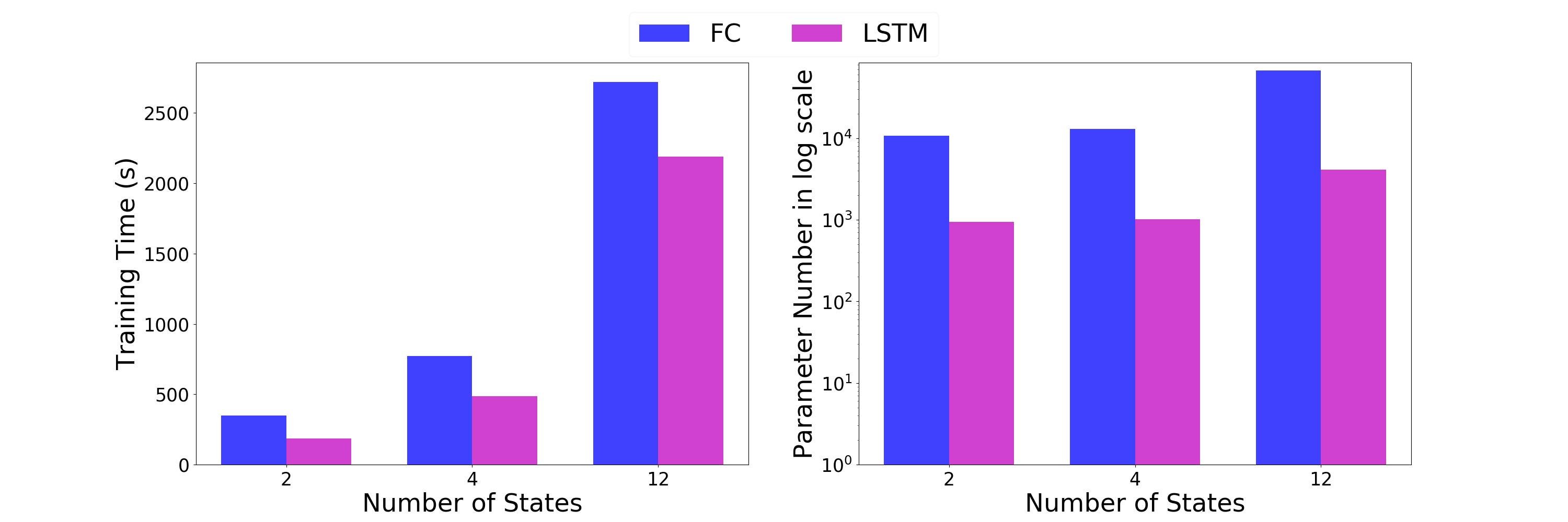
Figure 3: Comparing neural network training time (left) and number of trainable parameters (right) vs. state dimensionality for the proposed FC (Fig. 1) and LSTM (Fig. 2) network architectures.

The Deep FBSDE algorithm, as shown in Alg. 1, solves the finite time horizon control problem by approximating the gradient of the value function $\tilde{z}^{i}_{t}$ at every time step with a DNN parameterized by $\theta_{t}$. Note that the superscript $i$ is the batch index, and the batch-wise calculation can be implemented in parallel. The initial value $\tilde{y}^{i}_{0}$ and its gradient $\tilde{z}^{i}_{0}$ are parameterized by trainable variables $\phi$ and are randomly initialized. The optimal control action is calculated using the discretized version of (6) (or (26) for the control constrained case). The dynamics $\tilde{x}$ and value function $\tilde{y}$ are propagated using the Euler integration scheme, as shown in the algorithm. The function $h$ is calculated using (13) (or (28) for the control constrained case). The predicted final value $\tilde{y}^{i}_{N}$ is compared against the true final value ${y^{*}_{N}}^{i}$ to calculate the loss. The networks can be trained with any one of the variants of Stochastic Gradient Descent (SGD) such as the Adam optimizer [27] until convergence with custom learning rate scheduling. The trained networks can then be used to predict the optimal control at every time step starting from the given initial condition $\xi$.

Network Architectures: The network architectures illustrated in figures 1 and 2, are extensions of the network introduced in [24] (refer to fig. 4 in the paper). The neural network architectures in figures 1 and 2 have additional connections (highlighted by boldfaced arrows) that use the predicted gradient of the value function at every time step to compute and apply an optimal feedback control. An architecture similar to fig. 1 was introduced in [28] to solve model-based Reinforcement Learning (RL) problems posed as finite time horizon SOC problems. This consisted of a FC network at every timestep to predict an action as a function of the current state. The networks were stacked together to form one large deep network which was trained in an end-to-end fashion with the goal of minimizing the accumulated cost (or maximizing accumulated reward). In contrast, the network architecture in fig. 1 uses the explicit form of the optimal feedback control (eq. (6) or eq. (26)) at every timestep calculated using the value function gradient predicted by the network. In addition, we use the prediction to propagate the value function according to the BSDE (19) and minimize the difference between the propagated value function and the true value function at the final state. This, however, creates a new path for gradient backpropagation through time [29] which introduces both advantages and challenges for training the networks. The advantage being a direct influence of the weights on the state cost $q(\tilde{x}_{t})$ leading to accelerated convergence. Nonetheless, this passage also leads to the vanishing gradient problem, which has been known to plague training of Recurrent Neural Networks for long sequences (or time horizons).

To tackle this problem, we propose a new LSTM-based network architecture, as shown in fig. 2, which can effectively deal with the vanishing gradient problem [30] as it allows for the gradient to flow unchanged. Additionally, since the weights are shared across all time steps, the total number of parameters to train is far less than the FC structure. These features allows the algorithm to scale to optimal problems of long time horizons. Intuitively, one can also think of the use of LSTM as modeling the time evolution of $V_{\tilde{x}}$, in contrast to the FC structure, which acts independently at every time step.

V Simulation Results

We applied the Deep FBSDE controller to systems of pendulum, cartpole and quadcopter for the task of reaching a target final state. The trained networks are evaluated over 128 trials and the results are compared between the different network architectures for both the unconstrained and control constrained case. We use FC and LSTM to denote experiments with the network architectures in fig. 1 and 2 respectively. We use 2 layer FC and LSTM networks and tanh activation for all experiments, with $\Delta t=0.02\,s$. All experiments were conducted in TensorFlow [31] on an Intel i7-4820k CPU Processor. A comparison of training time and trainable parameter number is shown in fig. 3, where it is clear that the LSTM network saves at least 20% of training time and has much fewer parameters than the FC network.

In all trajectory plots, the solid line represents the mean trajectory, and shaded region shows the 95% confidence region. To differentiate between the 4 cases, we use blue for unconstrained FC, green for unconstrained LSTM, cyan for constrained FC and magenta for constrained LSTM.

V-A Pendulum

The algorithm was applied to the pendulum system for the swing-up task with a time horizon of 1.5 seconds. The equation of motion for the pendulum is given by

$$ml^{2}\ddot{\theta}+mgl\sin{\theta}+b\dot{\theta}=u.$$ (29)

The initial pendulum angle is 0 $radian$, and the target pendulum angle and rate are $\pi$ $radians$ and 0 $rad/s$ respectively. A maximum torque constraint of $u^{max}=10\;Nm$ is used for the control constrained cases.

Fig. 4 shows the state trajectories across the 4 case. It can be observed that the swing-up task is completed in all casess with low variance. However, the pole rate does not return to 0 for unconstrained FC, as compared to unconstrained LSTM. When the control is constrained, the pendulum angular rate becomes serrated for FC while remaining smooth for LSTM. This also more noticeable in the control torques (fig. 5). The control torques becomes very spiky for FC due to the independent networks at each time step. On the other hand, the hidden temporal connection within LSTM allows for smooth and optimally behaved control policy.

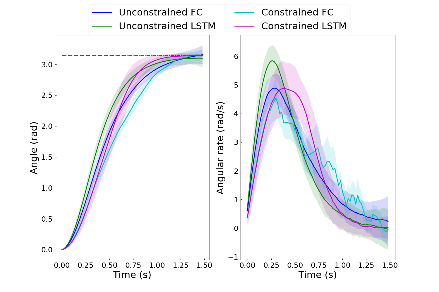
Figure 4: Pendulum states. Left: Pendulum Angle; Right: Pendulum Rate.

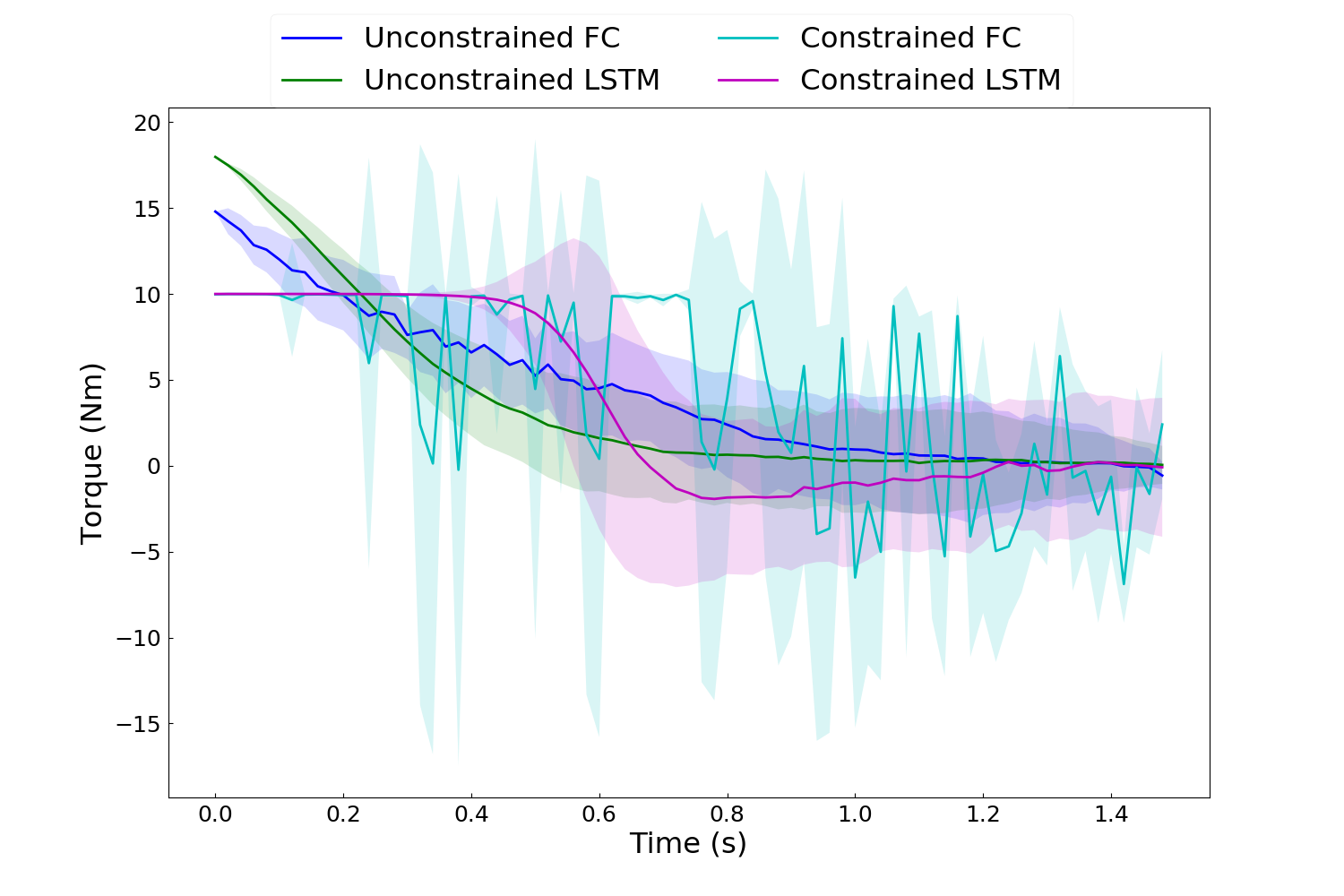
Figure 5: Pendulum controls.

V-B Cart Pole

The algorithm was applied to the cart-pole system for the swing-up task with a time horizon of 1.5 seconds. The equations of motion for the cart-pole are given by

$$2\ddot{x}+\ddot{\theta}\cos{\theta}-\dot{\theta}^{2}\sin{\theta}=u$$ (30)

$$\ddot{x}\cos{\theta}+\ddot{\theta}+\sin{\theta}=0.$$ (31)

The initial pole angle is 0 $radian$, and the target pole angle is $\pi$ $radians$ with target pole and cart velocities of 0 $rad/s$ and 0 $m/s$ respectively. Note that despite the target of 0 $m$ for cart position, we do not penalize non-zero cart position in training. A maximum force constraint of 10 $N$ is used for the control constrained case.

The cart-pole states are shown in fig. 6. Similar to the pendulum experiment, the swing-up task is completed with low variance acrossed all cases. Interestingly, when control is constrained, both FC and LSTM swing the pole in the direction opposite to target at first and utilize momentum to complete the task. Another interesting observation is that in the unconstrained case, the LSTM-policy is able to exploit long-term temporal connections to initially apply large controls to swing-up the pole and then focus on decelerating the pole for the rest of the time horizon, whereas the FC-policy appears to be more myopic resulting in a delayed swing-up action. Similar to the pendulum experiment, under control constraint the FC-policy results in sawtooth-like controls while the LSTM-policy outputs smooth control trajectories.

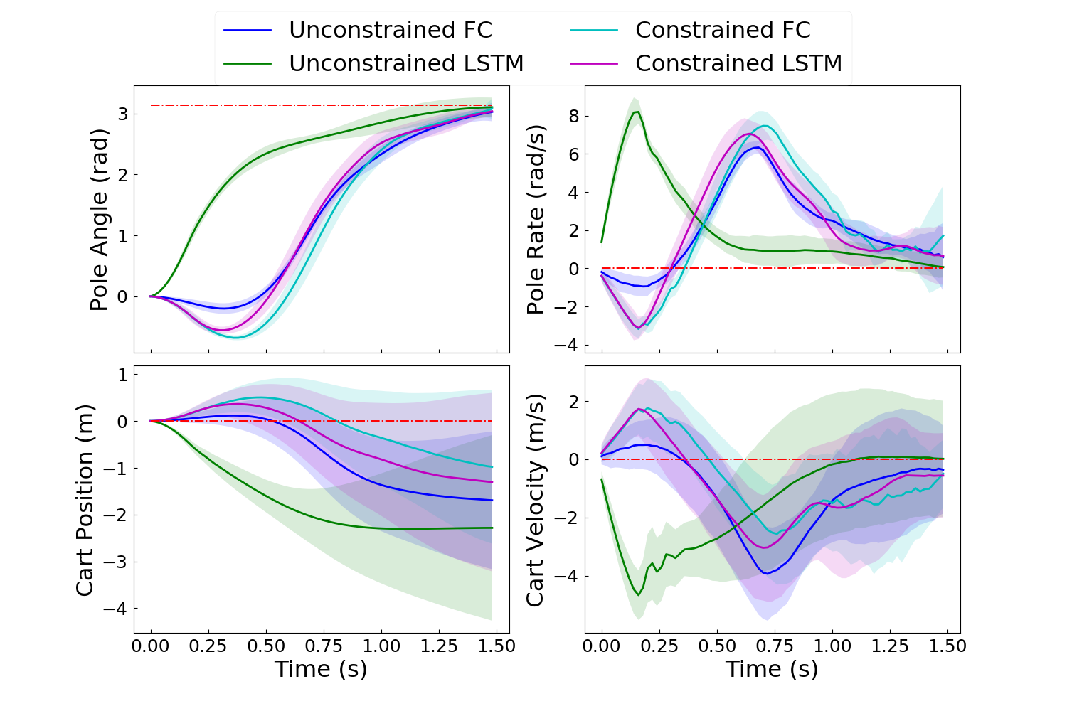
Figure 6: Cart Pole states. Top Left: Pole Angle; Top Right: Pole Rate; Bottom Left: Cart Position; Bottom Right: Cart Velocity.

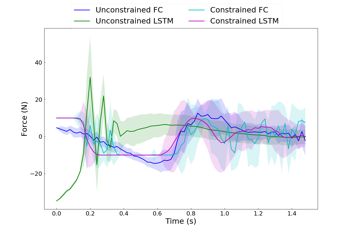
Figure 7: Cart Pole controls.

V-C Quadcopter

The algorithm was applied to the quadcopter system for the task of flying from its initial position to a target final position with a time horizon of 2 seconds. The quadcopter dynamics used is described in detail by Habib et al. [32]. The initial condition is 0 across all states, and the target is 1 $m$ upward, forward and to the right from the initial location with zero velocities and attitude. The controls are motor torques. A maximum torque constraint of 3 $Nm$ is imposed for the control constrained case.

This task required $N=100$ individual FC networks. After extensive experimentation, we conclude that tuning the FC-based policy becomes significantly difficult and cumbersome as the time horizon of the task increases. On the other hand, tuning our proposed LSTM-based policy was equivalent to that for the cart-pole and pendulum experiments. Moreover, the shared weights across all time steps results in faster build-times and run-times of the TensorFlow computational graph. As seen in the figures (8-10) from our experiments, the performance of the LSTM-based policies surpassed that of the FC-based policies (especially for the attitude states) due to exploiting long term temporal dependence and ease of tuning.

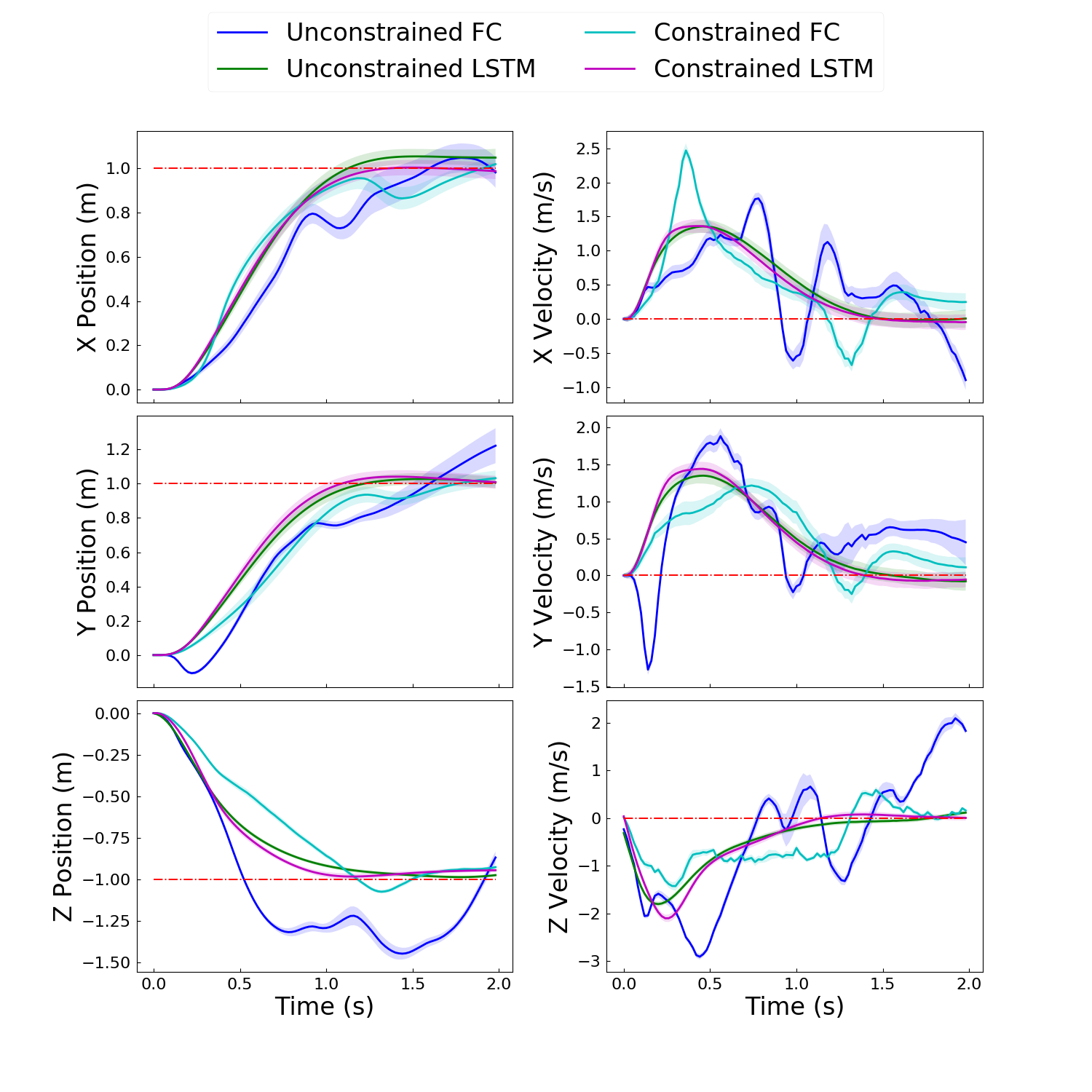
Figure 8: Quadcopter states. Top Left: X Position; Top Right: X Velocity; Middle Left: Y Position; Middle Right: Y Velocity; Bottom Left: Z Position; Bottom Right: Z Velocity.

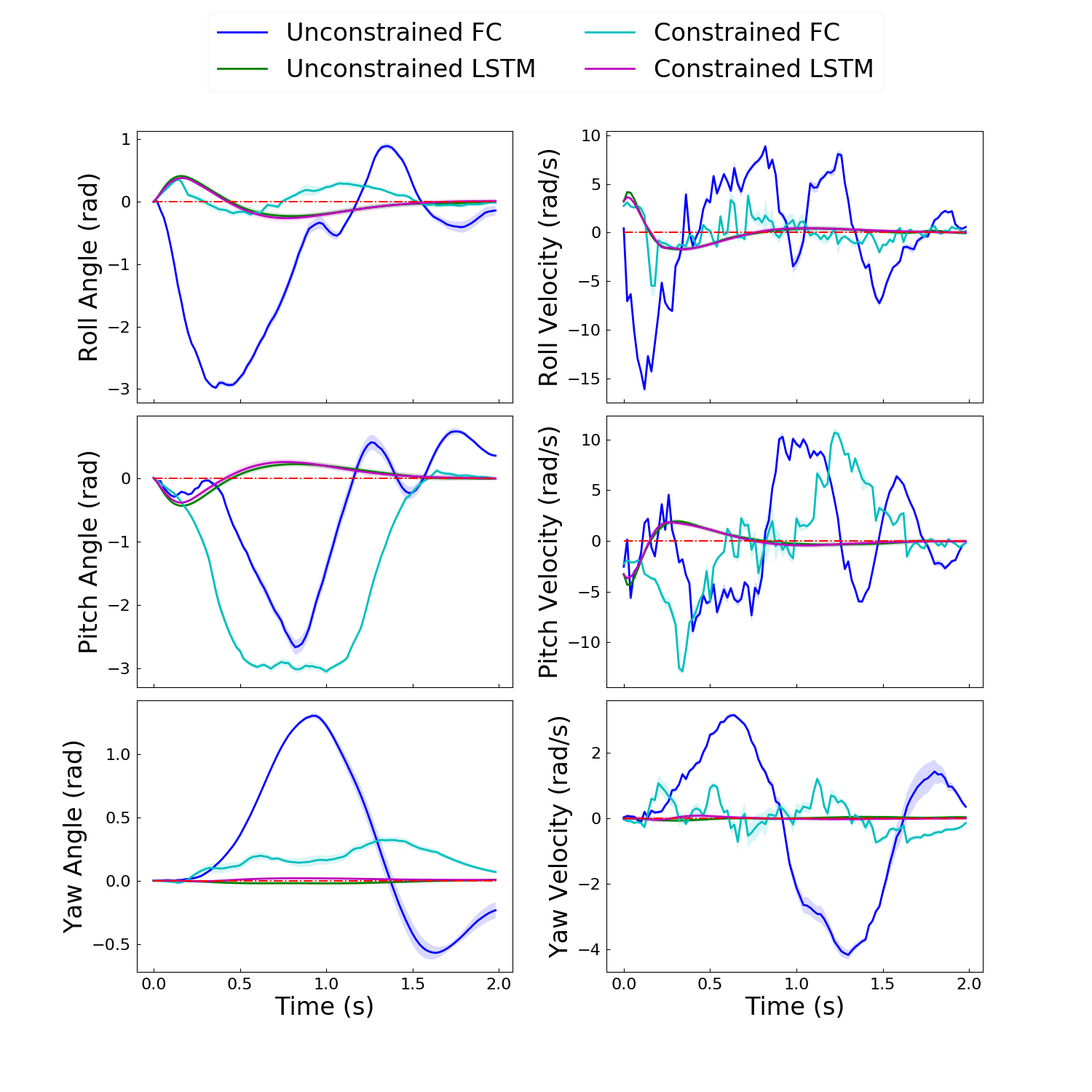
Figure 9: Quadcopter states. Top Left: Roll Angle; Top Right: Roll Velocity; Middle Left: Pitch Angle; Middle Right: Pitch Velocity; Bottom Left: Yaw Angle; Bottom Right: Yaw Velocity.

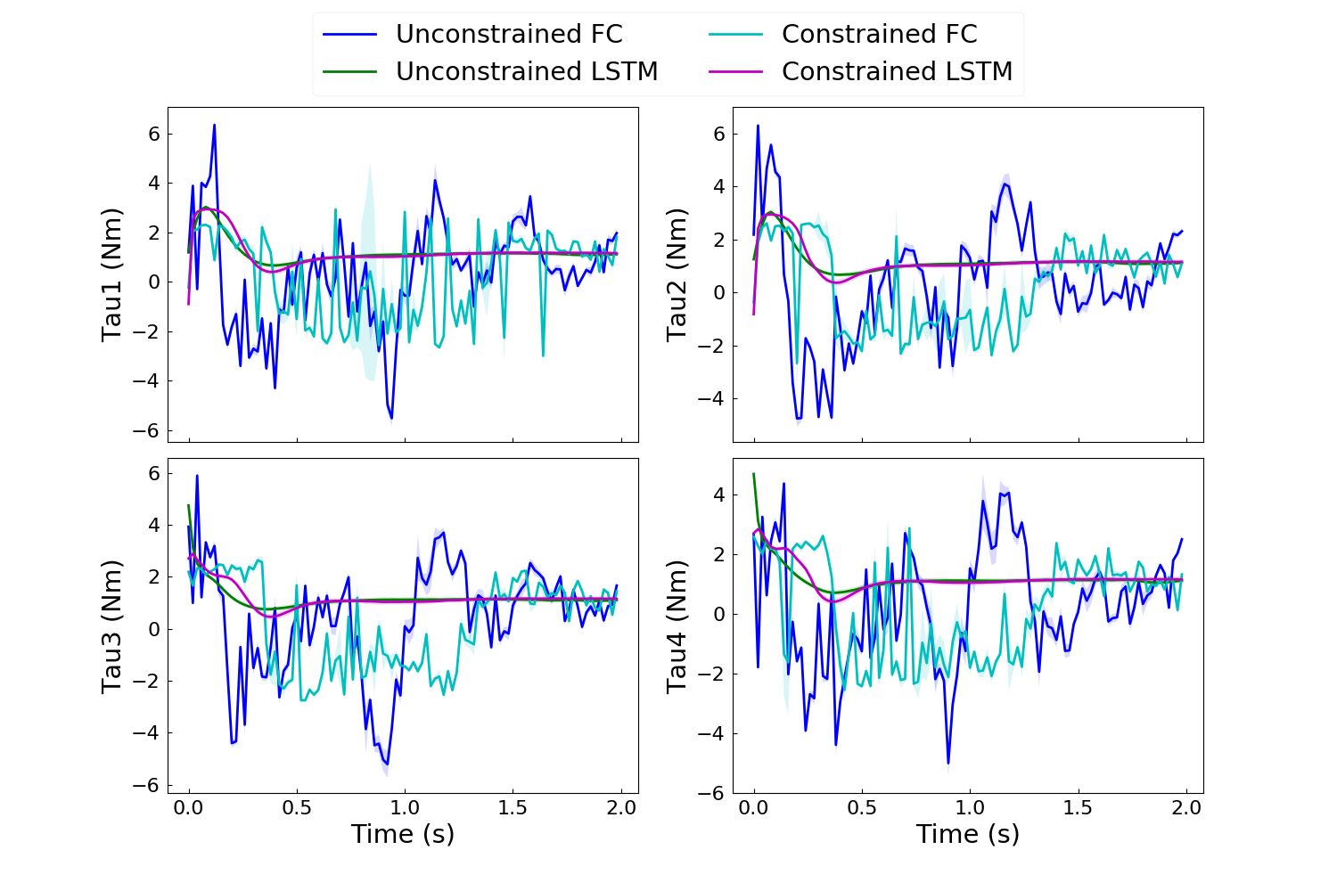
Figure 10: Quadcopter controls.

VI Conclusions

In this paper, we proposed the Deep FBSDE Control algorithm that utilizes fully connected and recurrent layers based on the LSTM network architecture. The proposed algorithm solves finite time horizon Stochastic Optimal Control problems for nonlinear systems with control-affine dynamics and constraints in the controls.

The architectures presented in this paper can be extended in many different ways, some of which include:

• Risk-Sensitive and Min-Max Stochastic Optimal Control: This type of Stochastic Optimal Control problems result in the so-called Hamilton-Jacobi-Bellman-Isaacs PDE. The min-max formulations are typically used to model stochastic disturbances with unknown mean. Solving these SOC problems will result in robust policies in robotics.

• Stochastic Optimal Control of systems with generalized stochasticities: For systems with Lévy and jump-diffusion noise, the resulting HJB equation is a partial-integro-differential equation. Stochastic models that include jump-diffusions could be used to model wind-gust or ground forces in terrestrial vehicles.

• Non-affine control dynamics: Very often in robotics dynamics are represented by function approximators such as DNNs or Gaussian Processes (GPs). This choice results in dynamics that are non-affine in controls. A potential new direction is to generalize the Deep FBSDE Control algorithm for such representations.

References

- Dai Pra et al. [1996-12-08] P. Dai Pra, L. Meneghini, and W. Runggaldier. Connections between stochastic control and dynamic games. Mathematics of Control, Signals, and Systems (MCSS), 9(4):303–326, 1996-12-08. URL http://dx.doi.org/10.1007/BF01211853.
- Fleming [1971] W.H. Fleming. Exit probabilities and optimal stochastic control. Applied Math. Optim, 9:329–346, 1971.
- Theodorou and Todorov [2012] E.A Theodorou and E. Todorov. Relative entropy and free energy dualities: Connections to path integral and kl control. In the Proceedings of IEEE Conference on Decision and Control, pages 1466–1473, Dec 2012. doi: 10.1109/CDC.2012.6426381.
- Theodorou [2015] E. A. Theodorou. Nonlinear stochastic control and information theoretic dualities: Connections, interdependencies and thermodynamic interpretations. Entropy, 17(5):3352, 2015.
- Williams et al. [2018] G. Williams, P. Drews, B. Goldfain, J. M. Rehg, and E. A. Theodorou. Information-theoretic model predictive control: Theory and applications to autonomous driving. IEEE Transactions on Robotics, 34(6):1603–1622, Dec 2018. ISSN 1552-3098. doi: 10.1109/TRO.2018.2865891.
- NVIDIA [Aug 31, 1999] NVIDIA. Nvidia launches the world’s first graphics processing unit: Geforce 256. Aug 31, 1999. URL https://www.nvidia.com/object/IO_20020111_5424.html.
- Bellman [2013] Richard Bellman. Dynamic programming. Courier Corporation, 2013.
- Theodorou et al. [2010] E. A. Theodorou, J. Buchli, and S. Schaal. A Generalized Path Integral Control Approach to Reinforcement Learning. J. Mach. Learn. Res., 11:3137–3181, December 2010. ISSN 1532-4435.
- Karatzas and Shreve [1991] I. Karatzas and S. E. Shreve. Brownian Motion and Stochastic Calculus (Graduate Texts in Mathematics). Springer, 2nd edition, August 1991. ISBN 0387976558.
- Yong and Zhou [1999] Jiongmin Yong and Xun Yu Zhou. Stochastic controls: Hamiltonian systems and HJB equations, volume 43. Springer Science & Business Media, 1999.
- Pardoux and Rascanu [2014] Etienne Pardoux and Aurel Rascanu. Stochastic Differential Equations, Backward SDEs, Partial Differential Equations, volume 69. 07 2014. doi: 10.1007/978-3-319-05714-9.
- Kharroubi and Pham [2015] Idris Kharroubi and Huyen Pham. Feynman-Kac representation for Hamilton-Jacobi-Bellman IPDE. Ann. Probab., 43(4):1823–1865, 07 2015. doi: 10.1214/14-AOP920. URL https://doi.org/10.1214/14-AOP920.
- Fabbri et al. [2017] Giorgio Fabbri, Fausto Gozzi, and Andrzej Swiech. Stochastic Optimal Control in Infinite Dimensions - Dynamic Programming and HJB Equations. Number 82 in Probability Theory and Stochastic Modelling. Springer, January 2017. URL https://hal-amu.archives-ouvertes.fr/hal-01505767. OS.
- Exarchos and Theodorou [2018] I. Exarchos and E. A. Theodorou. Stochastic optimal control via forward and backward stochastic differential equations and importance sampling. Automatica, 87:159–165, 2018.
- Exarchos and Theodorou [2016] I. Exarchos and E. A. Theodorou. Learning optimal control via forward and backward stochastic differential equations. In American Control Conference (ACC), 2016, pages 2155–2161. IEEE, 2016.
- Exarchos [2017] I. Exarchos. Stochastic Optimal Control-A Forward and Backward Sampling Approach. PhD thesis, Georgia Institute of Technology, 2017.
- Raissi et al. [2019] M Raissi, P Perdikaris, and GE Karniadakis. Physics-informed neural networks: A deep learning framework for solving forward and inverse problems involving nonlinear partial differential equations. Journal of Computational Physics, 378:686–707, 2019.
- Rudy et al. [2017] Samuel H Rudy, Steven L Brunton, Joshua L Proctor, and J Nathan Kutz. Data-driven discovery of partial differential equations. Science Advances, 3(4):e1602614, 2017.
- Pereira et al. [2018] M. Pereira, D. D. Fan, G. Nakajima An, and E. A. Theodorou. MPC-Inspired Neural Network Policies for Sequential Decision Making. arXiv preprint arXiv:1802.05803, 2018.
- Amos et al. [2018] Brandon Amos, Ivan Jimenez, Jacob Sacks, Byron Boots, and J. Zico Kolter. Differentiable MPC for End-to-end Planning and Control. Advances in Neural Information Processing Systems, 2018.
- Pan et al. [2018] Y. Pan, C. Cheng, K. Saigol, K. Lee, X. Yan, E. A. Theodorou, and B. Boots. Agile Off-Road Autonomous Driving Using End-to-End Deep Imitation Learning. Robotics: Science and Systems, 2018.
- Morton et al. [2018] Jeremy Morton, Antony Jameson, Mykel J Kochenderfer, and Freddie Witherden. Deep Dynamical Modeling and Control of Unsteady Fluid Flows. Advances in Neural Information Processing Systems 31, pages 9278–9288, 2018.
- Goodfellow et al. [2016] Ian Goodfellow, Yoshua Bengio, and Aaron Courville. Deep Learning. The MIT Press, 2016. ISBN 0262035618, 9780262035613.
- Han et al. [2018] Jiequn Han, Arnulf Jentzen, and Weinan E. Solving high-dimensional partial differential equations using deep learning. Proceedings of the National Academy of Sciences, 115(34):8505–8510, 2018. ISSN 0027-8424. doi: 10.1073/pnas.1718942115. URL https://www.pnas.org/content/115/34/8505.
- Girsanov [1960] Igor Vladimirovich Girsanov. On transforming a certain class of stochastic processes by absolutely continuous substitution of measures. Theory of Probability & Its Applications, 5(3):285–301, 1960.
- Exarchos et al. [2018] I. Exarchos, E. A. Theodorou, and P. Tsiotras. Stochastic -optimal control via forward and backward sampling. Systems & Control Letters, 118:101–108, 2018.
- Kingma and Ba [2014] Diederik P. Kingma and Jimmy Ba. Adam: A method for stochastic optimization. CoRR, abs/1412.6980, 2014. URL http://arxiv.org/abs/1412.6980.
- Han et al. [2016] Jiequn Han et al. Deep Learning Approximation for Stochastic Control Problems. arXiv preprint arXiv:1611.07422, 2016.
- Werbos [1990] Paul J Werbos. Backpropagation through time: what it does and how to do it. Proceedings of the IEEE, 78(10):1550–1560, 1990.
- Hochreiter and Schmidhuber [1997] Sepp Hochreiter and Jürgen Schmidhuber. LSTM can solve hard long time lag problems. pages 473–479, 1997.
- Abadi et al. [2015] Martín Abadi, Ashish Agarwal, Paul Barham, Eugene Brevdo, Zhifeng Chen, Craig Citro, Greg S. Corrado, Andy Davis, Jeffrey Dean, Matthieu Devin, Sanjay Ghemawat, Ian Goodfellow, Andrew Harp, Geoffrey Irving, Michael Isard, Yangqing Jia, Rafal Jozefowicz, Lukasz Kaiser, Manjunath Kudlur, Josh Levenberg, Dan Mané, Rajat Monga, Sherry Moore, Derek Murray, Chris Olah, Mike Schuster, Jonathon Shlens, Benoit Steiner, Ilya Sutskever, Kunal Talwar, Paul Tucker, Vincent Vanhoucke, Vijay Vasudevan, Fernanda Viégas, Oriol Vinyals, Pete Warden, Martin Wattenberg, Martin Wicke, Yuan Yu, and Xiaoqiang Zheng. TensorFlow: Large-scale machine learning on heterogeneous systems, 2015. URL http://tensorflow.org/. Software available from tensorflow.org.
- Habib et al. [2014] Maki K Habib, Wahied Gharieb Ali Abdelaal, Mohamed Shawky Saad, et al. Dynamic modeling and control of a quadrotor using linear and nonlinear approaches. 2014.