Primal-dual gap estimators for a posteriori error analysis of nonsmooth minimization problems

Abstract.

The primal-dual gap is a natural upper bound for the energy error and, for uniformly convex minimization problems, also for the error in the energy norm. This feature can be used to construct reliable primal-dual gap error estimators for which the constant in the reliability estimate equals one for the energy error and equals the uniform convexity constant for the error in the energy norm. In particular, it defines a reliable upper bound for any functions that are feasible for the primal and the associated dual problem. The abstract a posteriori error estimate based on the primal-dual gap is provided in this article, and the abstract theory is applied to the nonlinear Laplace problem and the Rudin-Osher-Fatemi image denoising problem. The discretization of the primal and dual problems with conforming, low-order finite element spaces is addressed. The primal-dual gap error estimator is used to define an adaptive finite element scheme and numerical experiments are presented, which illustrate the accurate, local mesh refinement in a neighborhood of the singularities, the reliability of the primal-dual gap error estimator and the moderate overestimation of the error.

1. Introduction

Many problems in various applications like partial differential equations, mechanics, imaging, and operations research can be formulated as convex minimization problems of the form

$$\inf_{u\in X}E(u)=\inf_{u\in X}F(Bu)+G(u)$$

with convex functionals $F,G$ and a bounded linear operator $B$. Examples are the nonlinear Laplace equation, the Rudin-Osher-Fatemi model for image denoising, obstacle problems or convex programming. Depending on the data and the geometry of the problem a solution $u\in X$ of the above minimization problem may suffer from singularities which can harm the convergence rate as the mesh size $h>0$ of a finite element method tends to zero. A well-known example for this phenomenon is the linear Laplace problem on the L-shaped domain. The geometry of the domain leads to a convergence rate of order $\mathcal{O}(h^{\gamma})$ instead of $\mathcal{O}(h)$ in the energy norm, where $0<\gamma<1$ and $\gamma$ depends on the angle at the reentrant corner. Singularities may also arise due to intrinsic properties of the functions in the underlying space $X$. An example is the space of functions with bounded variation $BV(\Omega)$, which allows for jumps along interfaces, which is of interest, e.g., in image processing to preserve sharp edges. Yet, these jumps cause problems in the finite element approximation of $BV$-functions.

One way to overcome these drawbacks is adaptive mesh refinement. The general procedure of adaptive routines is to compute an approximation of the minimizer in the discrete space with a given underlying triangulation, compute a posteriori error estimators on the basis of the computed approximation, refine the mesh locally where the error estimators are relatively large and to compute a new approximate solution corresponding to the new mesh. In this sense, adaptive methods are iterative numerical methods. The reader is referred to, e.g., [5, 1, 38, 50, 47] to get an overview of adaptive finite element methods.

The design of a posteriori error estimators is fundamental to adaptive finite element methods. Particularly, it is crucial that the error estimators define upper (reliability) and lower (efficiency) bounds for an appropriate measure of the error and that the constant in the upper bound is small and known. We will consider primal-dual gap error estimators which can be derived using duality theory from convex analysis. In the contributions [43, 41, 42, 40, 44, 45, 8, 12] these primal-dual gap error estimators have been introduced and used for various problems, e.g., elasto-plasticity and optimal transport. In [43] the primal-dual gap error estimator has been analyzed for general convex minimization problems with uniformly convex functionals and the relation to other a posteriori error estimators based on, e.g., residual and gradient recovery methods has been addressed. Yet, the numerical study of primal-dual gap error estimators has not been considered in any of those contributions. We will analyze primal-dual gap based error estimators for the nonlinear Laplace problem

$$E_{\Delta_{\sigma}}(u)=\frac{1}{\sigma}\int_{\Omega}|\nabla u|^{\sigma}\,{\mathrm{d}}x-\int_{\Omega}fu\,{\mathrm{d}}x\quad\longrightarrow\quad\text{Min.!}$$

with $1<\sigma<\infty$, which has also been addressed in [41] without a numerical study, and for the Rudin-Osher-Fatemi (ROF) model

$$E_{\rm rof}(u)=|{\rm D}u|(\Omega)+\frac{\alpha}{2}\|u-g\|_{L^{2}(\Omega)}^{2}\quad\longrightarrow\quad\text{Min.!}$$

with $|{\rm D}u|(\Omega)$ the total variation of $u$, which has been analyzed in, e.g., [8].

The nonlinear Laplace problem serves as a model problem for degenerate nonlinear systems. Results concerning the regularity of solutions, their approximation by finite elements and a priori error estimates can be found, e.g., in [30, 18, 7, 33, 32, 22, 21, 25, 24]. An important observation in the a priori error analysis was that the energy norm is not well suited for the analysis since optimal convergence rates can only be guaranteed under restrictive assumptions on the regularity of the solution, cf. [30, 18, 7, 33, 32]. It turned out that a so-called quasi-norm, which is a weighted $L^{2}$-norm of the gradient with a weight depending on the gradient and which has been introduced in [7], is more appropriate for the analysis of the nonlinear Laplacian, cf. [24, 20]. Particularly, the optimal convergence rate $\mathcal{O}(h)$ for P1 finite elements can be proven under much less restrictive regularity assumptions on the solution, cf. [25, 24, 20]. In [35, 34, 36] residual-based a posteriori error estimators have been proposed and reliability and efficiency has been established with respect to the quasi-norm. However, the involved constants are not explicitly available. Residual-based quasi-norm error estimators yielding explicit constants in the reliability estimate have been discussed in [16] under the assumption that the modulus of the gradient is greater than zero almost everywhere in the domain whereas the reliability and efficiency of quasi-norm error estimators based on gradient recovery techniques has been established in [17]. The convergence of an adaptive scheme with residual-based a posteriori error estimators has been proven in [49]. In [19, 13] the linear convergence and optimality of an adaptive method driven by residual-based quasi-norm error estimators has been proven. The involved constants particularly for the upper bound depend on the nonlinearity of the problem. In [27, 28] the error is measured in a residual flux-based dual norm and the a posteriori error estimator consists of a residual term, a diffusive flux term and a linearization term. Flux reconstruction techniques are presented to compute the error estimator and reliability (with constant one) and efficiency (with a constant independent of the nonlinearity of the problem) are shown. Particular focus is on the balance of linearization and discretization errors.

The ROF model serves as a prototype for $BV$-regularized minimization problems with applications, e.g., in image processing (cf. [46, 4]) and mechanics (cf. [48]). A primal-dual gap error estimator has been proposed to define an adaptive algorithm for the ROF problem in [8], which has proven to accurately detect the a priori unknown jump sets of the minimizer yielding locally refined meshes in a neighborhood of the jump sets. Therein, a finite element method has been proposed where the primal and dual problem have been discretized with continuous, elementwise affine finite elements. However, the approximation of the dual ROF problem by continuous finite elements is suboptimal since the dual ROF problem is posed on $H_{\rm N}(\operatorname{div};\Omega)$. This is reflected in the experiments in  [8] where oscillations of the approximations along the interface can be observed.

The advantage of primal-dual gap error estimators is that they are applicable to a large class of convex minimization problems and naturally yield upper bounds for the energy difference between the energy of an arbitrary admissible test function and the optimal energy with constant one. In case of $F$ or $G$ being strongly convex (or coercive) they also define upper bounds for some appropriate error measure with a constant depending on the coercivity constant. Particularly, they define reliable upper bounds independently of the iterative solver used to approximate discrete solutions to the primal and dual problem, i.e., the primal-dual gap error estimator can be evaluated at any two feasible functions for the primal and the dual problem to obtain an upper bound for the error. Last but not least, the functionals $F$ and $G$ need not be assumed to be differentiable and there does not need to exist a variational formulation of the primal problem to establish the reliability of the primal-dual gap error estimators.

In this paper we will consider primal-dual gap error estimators for both the nonlinear Laplace problem and the ROF problem. While in [41] the primal-dual gap error estimator has been considered for the nonlinear Laplacian, the discretization and numerical implementation is missing. Furthermore, noting that the dual problem corresponding to the nonlinear Laplace problem is given by a smooth, linearly constrained optimization problem a modified error estimator, which is an upper bound for the primal-dual gap error estimator, is suggested in [41] allowing for dual test functions that do not satisfy the linear constraint. We will consider the “original” primal-dual gap error estimator to control the quasi-norm used in [7, 19]. In particular, the primal-dual gap error estimator $\eta_{\rm pd}$ can be used to improve the reliability estimate for the convergent, reliable and efficient residual-based error estimator $\eta_{\rm res}$ analyzed in [19, 13], i.e., defining $\eta_{\rm com}=\min\{\eta_{\rm pd},\eta_{\rm res}\}$ we obtain a reliable, robust, efficient and convergent error estimator. Continuous, piecewise affine finite elements are used for the discretization of the primal nonlinear Laplace problem and the ROF problem posed in $W^{1,\alpha}(\Omega)$ and $BV(\Omega)\cap L^{2}(\Omega)$, respectively. The dual problems are posed in $W^{\beta}(\operatorname{div};\Omega)$, $\beta=\alpha/(\alpha-1)$, and $H_{\rm N}(\operatorname{div};\Omega)$ in case of the nonlinear Laplacian and the ROF problem, respectively. In both cases we use the Brezzi-Douglas-Marini finite element (cf.  [14]), which consists of discontinuous piecewise affine vector fields with continuous normal components across interelement sides, for the discretization. This is in contrast to the discretization in [8] where the dual ROF problem has been discretized with continuous, piecewise affine vector fields, which is known to be problematic in, e.g., the discretization of the dual formulation of the linear Laplacian with mixed finite elements. Particularly, oscillations are observed in the approximation of $u$ along the interface, cf. Section 6. The discrete optimization problems related to the primal and the dual problems are solved using the Variable-Alternating Direction Method of Multipliers (Variable-ADMM) proposed in [10] which is an operator splitting method with variable step sizes.

The paper is organized as follows. In Section 2 we introduce the notation, important function spaces and finite element spaces and state some approximation results. The abstract primal-dual gap error estimator and a posteriori error estimate are the subject of Section 3. In Sections 4 and 5 we state the nonlinear Laplace problem and the ROF problem, respectively, and the associated dual problems, summarize a priori and a posteriori error estimates and briefly address the numerical solution of the discrete primal and dual problems. Finally, we present in Section 6 our numerical results for both problems for examples for which the exact solutions are explicitly available.

Let us remark that this article is part of the thesis [37], in which certain arguments have been elaborated.

2. Preliminaries

2.A. Function spaces and convex analysis

We let $\Omega\subset\mathbb{R}^{d}$,  $d=2,3$, be a bounded, polygonal Lipschitz domain with Dirichlet boundary $\Gamma_{\rm D}$ and Neumann boundary $\Gamma_{\rm N}$ such that $\partial\Omega=\Gamma_{\rm D}\cup\Gamma_{\rm N}$. The $L^{2}$-norm on $\Omega$ is denoted by $\|\cdot\|$ and is induced by the scalar product

$$(v,w):=\int_{\Omega}v\cdot w\,{\mathrm{d}}x$$

for scalar functions or vector fields $v,w\in L^{2}(\Omega;\mathbb{R}^{r})$, $r\in\{1,d\}$, and we write $|\cdot|$ for the Euclidean norm.
For $s\geq 0$ and $\sigma\geq 1$ we let $W^{s,\sigma}(\Omega;\mathbb{R}^{r})$ be the standard Sobolev space with norm $\|\cdot\|_{W^{s,\sigma}(\Omega)}$ and seminorm $|\cdot|_{W^{s,\sigma}(\Omega)}$ with differentiability exponent $s$ and integrability exponent $\sigma$. The subspace $W_{\rm D}^{s,\sigma}(\Omega;\mathbb{R}^{r})$ consists of all functions in $W^{s,\sigma}(\Omega;\mathbb{R}^{r})$ that vanish on $\Gamma_{\rm D}$ for $s\geq 1$ in the sense of traces. If $s=0$ we write $L^{\sigma}(\Omega;\mathbb{R}^{r})$ instead of $W^{s,\sigma}(\Omega;\mathbb{R}^{r})$.
Finally, for $\sigma^{\prime}\geq 1$, we denote by $W^{\sigma^{\prime}}(\operatorname{div};\Omega)$ the function space consisting of all vector fields $p\in L^{\sigma^{\prime}}(\Omega;\mathbb{R}^{d})$ such that there exists a function $f\in L^{\sigma^{\prime}}(\Omega)$ with

$$\int_{\Omega}p\cdot\nabla\varphi\,{\mathrm{d}}x=-\int_{\Omega}f\varphi\,{\mathrm{d}}x$$

for all continuously differentiable, compactly supported functions $\varphi\in C_{c}^{1}(\Omega)$. If such a function $f\in L^{\sigma^{\prime}}(\Omega)$ exists, we write $\operatorname{div}p=f$. The space $W^{\sigma^{\prime}}(\operatorname{div};\Omega)$ is equipped with the norm

$$\|\cdot\|_{W^{\sigma^{\prime}}(\operatorname{div};\Omega)}=\|\cdot\|_{L^{\sigma^{\prime}}(\Omega)}+\|\operatorname{div}\cdot\|_{L^{\sigma^{\prime}}(\Omega)}.$$

Furthermore, we denote by $W_{\rm N}^{\sigma^{\prime}}(\operatorname{div};\Omega)$ all elements of $p\in W^{\sigma^{\prime}}(\operatorname{div};\Omega)$ with $p\cdot n=0$ on $\Gamma_{\rm N}$ in distributional sense, i.e.,

$$\langle p\cdot n,u\rangle=\int_{\Omega}p\cdot\nabla u\,{\mathrm{d}}x+\int_{\Omega}u\operatorname{div}p\,{\mathrm{d}}x=0$$

for all $u\in W_{\rm D}^{1,\sigma}(\Omega)$, where $\sigma\geq 1$ is the dual exponent to $\sigma^{\prime}\geq 1$, i.e., $1/\sigma+1/\sigma^{\prime}=1$. If $\sigma^{\prime}=2$ we write $H(\operatorname{div};\Omega)$ instead of $W^{2}(\operatorname{div};\Omega)$, and accordingly $H_{\rm N}(\operatorname{div};\Omega)$ instead of $W_{\rm N}^{2}(\operatorname{div};\Omega)$.

For the general, abstract a posteriori error estimate we will work with two reflexive Banach spaces $X$ and $Y$ equipped with the norms $\|\cdot\|_{X}$ and $\|\cdot\|_{Y}$, respectively. We denote their duals by $X^{\prime}$ and $Y^{\prime}$ and the corresponding duality pairings by $\langle\cdot,\cdot\rangle_{X^{\prime},X}$ and $\langle\cdot,\cdot\rangle_{Y^{\prime},Y}$, respectively. The double duals $X^{\prime\prime}$ and $Y^{\prime\prime}$ are identified with $X$ and $Y$, respectively. If $X$ is a Hilbert space with inner product $(\cdot,\cdot)_{X}$, we identify the dual $X^{\prime}$ with $X$. Given a bounded linear operator $B:X\to Y$ we denote by $B^{\prime}:Y^{\prime}\to X^{\prime}$ its adjoint. For proper, convex and lower-semicontinuous functionals $F:Y\to\mathbb{R}\cup\{\infty\}$ and $G:X\to\mathbb{R}\cup\{\infty\}$ the subdifferentials $\partial G(u)\subset X^{\prime}$ at $u\in X$ and $\partial F(p)\subset Y^{\prime}$ at $p\in Y$ are defined by

$$\begin{split}\partial G(u)&=\{w\in X^{\prime}:\;\langle w,v-u\rangle_{X^{\prime},X}+G(u)\leq G(v)\quad\text{for all }v\in X\},\\ \partial F(p)&=\{\lambda\in Y^{\prime}:\;\langle\lambda,q-p\rangle_{Y^{\prime},Y}+F(p)\leq F(q)\quad\text{for all }q\in Y\}.\end{split}$$

Possible coercivity of the functionals $F$ and $G$ is characterized by non-negative mappings $\varrho_{F}:Y\times Y\to\mathbb{R}_{+}$ and $\varrho_{G}:X\times X\to\mathbb{R}_{+}$ such that for $w\in\partial G(u)$ and $\lambda\in\partial F(p)$ we have

(1) $$\begin{split}\langle w,v-u\rangle_{X^{\prime},X}+G(u)+\varrho_{G}(v,u)&\leq G(v)\quad\text{for all }v\in X,\\ \langle\lambda,q-p\rangle_{Y^{\prime},Y}+F(p)+\varrho_{F}(q,p)&\leq F(q)\quad\text{for all }q\in Y.\end{split}$$

This can be regarded as a generalization of the notion of uniform convexity and strong convexity. The existence of non-trivial $\varrho_{G}$ or $\varrho_{F}$ will induce an error measure for which we establish primal-dual gap error estimates. For the a posteriori error analysis we will need the Fenchel conjugates $F^{*}$ and $G^{*}$, which are defined by

$$F^{*}(q)=\sup_{p\in Y}\langle q,p\rangle_{Y^{\prime},Y}-F(p),\quad G^{*}(v)=\sup_{u\in X}\langle v,u\rangle_{X^{\prime},X}-G(u).$$

These are used to convert the primal problems into dual problems.

2.B. Finite element spaces

We let $(\mathcal{T}_{h})_{h>0}$ be a family of regular triangulations of $\Omega$. The set $\mathcal{S}_{h}$ consists of all edges ($d=2$) or faces ($d=3$) of elements of $\mathcal{T}_{h}$ and $\mathcal{N}_{h}$ denotes the set of nodes of $\mathcal{T}_{h}$. The elementwise constant mesh size function $h_{\mathcal{T}}\in\mathcal{L}^{\infty}(\Omega)$ is defined by

$$h_{\mathcal{T}}|_{T}=h_{T}=\operatorname{diam}(T)$$

for all $T\in\mathcal{T}_{h}$. In the context of locally refined meshes we employ the average mesh size

$$\overline{h}=|\mathcal{N}_{h}|^{-1/d}$$

defined with the cardinality $|\mathcal{N}_{h}|$ of $\mathcal{N}_{h}$. Throughout the paper $c$ will denote a generic, positive and mesh-independent constant.
For an integer $k\geq 0$ and a triangle $T\in\mathcal{T}_{h}$ let $P_{k}(T)$ be the space of polynomials on $T$ with total degree at most $k$. We then consider for $r\in\{1,d\}$ the finite element spaces

$$\mathcal{S}^{k}(\mathcal{T}_{h})^{r}:=\bigl{\{}v_{h}\in C(\overline{\Omega};\mathbb{R}^{r}):\;v_{h}|_{T}\in P_{k}(T)^{r}\text{ for all }T\in\mathcal{T}_{h}\bigr{\}}$$

and

$$\mathcal{L}^{k}(\mathcal{T}_{h})^{r}:=\big{\{}q_{h}\in L^{1}(\Omega;\mathbb{R}^{r}):\;q_{h}|_{T}\in P_{k}(T)^{r}\text{ for all }T\in\mathcal{T}_{h}\big{\}}.$$

For an elementwise continuous function $v\in C(\mathcal{T}_{h})$ the operator

$$\widehat{\mathcal{I}}_{h}:C(\mathcal{T}_{h})\to\mathcal{L}^{1}(\mathcal{T}_{h})$$

is defined by the elementwise application of the standard nodal interpolation operator $\mathcal{I}_{h}:C(\overline{\Omega})\to\mathcal{S}^{1}(\mathcal{T}_{h})$. Note that $\widehat{\mathcal{I}}_{h}|_{C(\overline{\Omega})}=\mathcal{I}_{h}$. With the nodal basis $\{\varphi_{z}:\;z\in\mathcal{N}_{h}\}\subset\mathcal{S}^{1}(\mathcal{T}_{h})$ the bilinear form

$$(v,w)_{h}:=\int_{\Omega}\widehat{\mathcal{I}}_{h}(vw)\,{\mathrm{d}}x=\sum_{T\in\mathcal{T}_{h}}\sum_{z\in\mathcal{N}_{h}\cap T}\beta_{z}^{T}v|_{T}(z)w|_{T}(z)$$

for $v,w\in\mathcal{L}^{1}(\mathcal{T}_{h})$, where $\beta_{z}=\int_{T}\varphi_{z}\,{\mathrm{d}}x$, defines an inner product on $\mathcal{L}^{1}(\mathcal{T}_{h})$. This mass lumping will allow for the nodewise solution of certain nonlinearities. We have the relation

$$\|v_{h}\|\leq\|v_{h}\|_{h}\leq(d+2)^{1/2}\|v_{h}\|$$

for all $v_{h}\in\mathcal{L}^{1}(\mathcal{T}_{h})$, cf. [9, Lemma 3.9].

For completeness we provide the next lemma which states that $\mathcal{S}^{1}(\mathcal{T}_{h})^{d}$ is dense in $W^{\beta}(\operatorname{div};\Omega)$.

Lemma 2.1.

Let $p\in W^{\beta}(\operatorname{div};\Omega)$. For every $\varepsilon>0$ there exists $h(\varepsilon)>0$ such that for all $h\leq h(\varepsilon)$ there exists a function $q_{h}\in\mathcal{S}^{1}(\mathcal{T}_{h})^{d}$ with

$$\|p-q_{h}\|_{W^{\beta}(\operatorname{div};\Omega)}<\varepsilon.$$

Proof.

Since $C^{\infty}(\overline{\Omega};\mathbb{R}^{d})$ is dense in $W^{\beta}(\operatorname{div};\Omega)$, there exists for given $\varepsilon>0$ a function $q\in C^{\infty}(\overline{\Omega};\mathbb{R}^{d})$ with

$$\|p-q\|_{H(\operatorname{div};\Omega)}<\varepsilon/2.$$

Standard nodal interpolation estimates yield

$$\|q-\mathcal{I}_{h}q\|_{W^{\beta}(\operatorname{div};\Omega)}\leq\|q-\mathcal{I}_{h}q\|_{W^{1,\beta}(\Omega;\mathbb{R}^{d})}\leq ch|q|_{W^{2,\infty}(\Omega;\mathbb{R}^{d})}.$$

Now let $h$ be such that

$$\|q-\mathcal{I}_{h}q\|_{W^{\beta}(\operatorname{div};\Omega)}<\varepsilon/2.$$

Choosing $q_{h}=\mathcal{I}_{h}q$ and using the triangle inequality yields the assertion. ∎

For an element $T\in\mathcal{T}_{h}$ and $p_{h}\in P_{k}(T)^{r}$ we have by an inverse estimate

$$\|p_{h}\|_{L^{2}(T)}^{2}\leq ch_{T}^{2\min\{0,d/2-d/\alpha\}}\|p_{h}\|_{L^{\alpha}(T)}^{2},$$

cf. [15]. Hence, we may introduce for $1\leq\alpha<2$ the weighted $L^{2}$-inner product

$$(p_{h},q_{h})_{w_{\alpha}}=(h_{\mathcal{T}}^{d(2/\alpha-1)}p_{h},q_{h})$$

for $p_{h},q_{h}\in\mathcal{L}^{k}(\mathcal{T}_{h})$. Its induced norm then has the property $\|\cdot\|_{w_{\alpha}}\leq c\|\cdot\|_{L^{\alpha}(\Omega)}$ on $\mathcal{L}^{k}(\mathcal{T}_{h})$.

Let us finally introduce the so called Brezzi-Douglas-Marini (BDM) finite element space which is given by

$$\mathcal{BDM}(\Omega)=\mathcal{L}^{1}(\mathcal{T}_{h})^{d}\cap H(\operatorname{div};\Omega)\subset H(\operatorname{div};\Omega),$$

cf. [14]. For an element $T\in\mathcal{T}_{h}$ we can define a local interpolation operator $\Pi_{h,T}:H^{1}(T)^{d}\to P_{1}(T)^{d}$ by

$$\int_{S}q\cdot n\psi\,{\mathrm{d}}s=\int_{S}\Pi_{h,T}q\cdot n\psi\,{\mathrm{d}}s$$

for all sides $S\in\mathcal{S}_{h}\cap T$ of the element $T$ and all affine functions $\psi\in P_{1}(S)$ on $S$. Note that the interpolation operator is well-defined also for less regular functions, e.g., for $q\in H(\operatorname{div};T)\cap L^{\gamma}(T;\mathbb{R}^{d})$ with $\gamma>2$, cf. [14]. The global interpolation operator $\Pi_{h}:H^{1}(\Omega)^{d}\to\mathcal{BDM}(\Omega)$ is then defined by

$$(\Pi_{h}q)|_{T}=\Pi_{h,T}(q|_{T})$$

and, in particular, $\Pi_{h}q\in\mathcal{BDM}(\Omega)\subset H(\operatorname{div};\Omega)$. For more details on $H(\operatorname{div};\Omega)$-conforming finite element spaces we refer the reader to [14].

3. Abstract error estimate

In the following we recap the existing results on abstract a posteriori error estimation for convex minimization problems and refer to [40, 43, 41, 8] for further details.

Let $F:Y\to\mathbb{R}\cup\{\infty\}$ and $G:X\to\mathbb{R}\cup\{\infty\}$ be proper, convex and lower-semicontinuous functionals and $B:X\to Y$ be bounded and linear. Under these hypothesis there holds $F=(F^{*})^{*}$ and we obtain

$$\begin{split}\inf_{u\in X}E(u)&=\inf_{u\in X}F(Bu)+G(u)\\ &=\inf_{u\in X}\sup_{p\in Y^{\prime}}\;\langle p,Bu\rangle_{Y^{\prime},Y}-F^{*}(p)+G(u)\\ &\geq\sup_{p\in Y^{\prime}}\inf_{u\in X}\;-F^{*}(p)+\langle p,Bu\rangle_{Y^{\prime},Y}+G(u)\\ &=\sup_{p\in Y^{\prime}}-\sup_{u\in X}\;F^{*}(p)+\langle-B^{\prime}p,u\rangle_{X^{\prime},X}-G(u)\\ &=\sup_{p\in Y^{\prime}}\;-F^{*}(p)-G^{*}(-B^{\prime}p)\\ &=:\sup_{p\in Y^{\prime}}D(p).\end{split}$$

Hence, the dual formulation seeks a maximizer $p\in Y^{\prime}$ for $D$. Particularly, we have the weak duality relation

(2) $$E(v)\geq D(q)$$

for all $v\in X$ and $q\in Y^{\prime}$. If $u\in X$ is a minimizer for $E$, the necessary optimality condition reads

$$0\in\partial E(u).$$

With a nonnegative coercivity functional $\varrho_{E}:X\times X\to[0,\infty)$ this is equivalent to

(3) $$\varrho_{E}(v,u)+E(u)\leq E(v)$$

for all $v\in X$. A combination of (2) and (3) yields the following abstract a posteriori error estimate.

Proposition 3.1 (Primal-dual gap estimates).

Let $X_{h}\subset X$ and $Y_{h}\subset Y^{\prime}$ and $u\in X$ and $u_{h}\in X_{h}$ be minimial for $E$ in $X$ and $X_{h}$, respectively. We then have the a priori error estimate

$$\varrho_{E}(u,u_{h})\leq E(u_{h})-E(u)\leq\inf_{v_{h}\in X_{h}}E(v_{h})-E(u).$$

For any $w_{h}\in X_{h}$ and $q_{h}\in Y_{h}$ we have with $\eta(w_{h},q_{h}):=(E(w_{h})-D(q_{h}))^{1/2}$ the a posteriori error estimate

$$\varrho_{E}(u,u_{h})\leq\eta^{2}(w_{h},q_{h}).$$

Proof.

The a priori error estimate is a direct consequence of (3). Using the optimality (3) of $u\in X$, the weak duality (2) and $Y_{h}\subset Y^{\prime}$ we then obtain

$$\varrho_{E}(u,u_{h})\leq E(w_{h})-E(u)\leq E(u_{h})-\sup_{p\in Y^{\prime}}D(p)\leq E(w_{h})-D(q_{h}),$$

which concludes the proof. ∎

Remarks 3.2.

1. Note that in case of strong duality, i.e., there holds equality in (2), the a posteriori error estimate stated in Proposition 3.1 is sharp in the sense that if we use $w_{h}=u$ and $q_{h}=p$ in $\eta$ with $u\in X$ and $p\in Y^{\prime}$ being solutions to the primal and the dual problem, respectively, we have

$$\eta^{2}(u,p)=E(u)-D(p)=\inf_{v\in X}E(v)-\sup_{q\in Y^{\prime}}D(q)=0.$$

Sufficient for strong duality is that there exists $w\in X$ with $F(Bw)<\infty$, $G(w)<\infty$ and $F$ being continuous at $Bw$. In this case the solutions are related by the inclusions

$$-B^{\prime}p\in\partial G(u),\quad p\in\partial F(Bu),$$

cf. [26], which are equivalent to the variational inequalities

$$\begin{split}\langle-B^{\prime}p,v-u\rangle_{X^{\prime},X}+\varrho_{G}(v,u)+G(u)&\leq G(v),\\ \langle p,Bv-Bu\rangle_{Y^{\prime},Y}+\varrho_{F}(Bv,Bu)+F(Bu)&\leq F(Bv).\end{split}$$

Adding both inequalities gives (3) with

$$\varrho_{E}(v,u)=\varrho_{F}(Bv,Bu)+\varrho_{G}(v,u),$$

which serves as an error measure.
2. Let us emphasize that for the derivation of the reliability estimate for the primal-dual gap error estimator $\eta$ we did not need to make any assumptions on the differentiability of the functionals $F$ and $G$.
3. One is free in the construction of feasible functions $w_{h}\in X_{h}$ and $q_{h}\in Y_{h}$ to define the error estimator $\eta(w_{h},q_{h})$. We will use the Variable-ADMM introduced in [10] to approximately solve the primal and the dual problem for the nonlinear Laplace problem and the ROF problem. However, feasible functions, e.g., for the dual problem, may be constructed using other techniques like gradient recovery or flux reconstruction techniques, if they are applicable for the specific problem. The relation between primal-dual gap error estimators and other error estimators is discussed in [43] for a certain class of convex minimization problems.

4. Nonlinear Laplace equation

4.A. Primal and dual formulation

The nonlinear Laplace problem seeks for $\sigma\in(1,\infty)$, $\sigma^{\prime}=\sigma/(\sigma-1)$, $f\in L^{\sigma^{\prime}}(\Omega)$, $g\in L^{\sigma^{\prime}}({\Gamma_{\rm N}})$, $\widetilde{u}_{\rm D}\in W^{1,\sigma}(\Omega)$ and $u_{\rm D}=\widetilde{u}_{\rm D}|_{\Gamma_{\rm D}}$ a function $u\in W^{1,\sigma}(\Omega)$ which is minimal for

$$E_{\Delta_{\sigma}}(u)=\frac{1}{\sigma}\int_{\Omega}|\nabla u|^{\sigma}\,{\mathrm{d}}x-\int_{\Omega}fu\,{\mathrm{d}}x-\int_{\Gamma_{\rm N}}gu\,{\mathrm{d}}s+I_{u_{\rm D}}(u|_{\Gamma_{\rm D}}).$$

The indicator functional $I_{u_{\rm D}}$ encodes the boundary condition $u|_{\Gamma_{\rm D}}=u_{\rm D}$ on ${\Gamma_{\rm D}}=\partial\Omega\setminus{\Gamma_{\rm N}}$. The minimization problem admits a unique minimizer, cf.  [30]. Minimization problems of the above structure arise in various areas of interest, e.g., nonlinear diffusion [39], nonlinear elasticity [2], and fluid mechanics [3, 6].

Let us make the following assumption that will simplify the presentation.

Assumption 4.1.

For ease of presentation we restrict to the case $g=0$ and $u_{\rm D}=0$ in what follows. We then omit the indicator functional $I_{u_{\rm D}}(u|_{\Gamma_{\rm D}})$ in the definition of $E_{\Delta_{\sigma}}$ and seek for a minimizer $u\in W_{\rm D}^{1,\sigma}(\Omega)$ instead.

The dual nonlinear Laplace problem seeks $p\in W_{\rm N}^{\sigma^{\prime}}(\operatorname{div};\Omega)$ that maximizes the functional

$$D_{\Delta_{\sigma}}(p):=-\frac{1}{\sigma^{\prime}}\int_{\Omega}|p|^{\sigma^{\prime}}\,{\mathrm{d}}x-I_{\{f\}}(-\operatorname{div}p).$$

The following result (cf. [41, Thm. 1]) shows that the dual nonlinear Laplace problem is in fact the dual problem to the primal nonlinear Laplace problem in the sense of Fenchel duality. It further ensures the strong duality between the primal and the dual nonlinear Laplace problem.

Theorem 4.2 (Strong duality).

There exists a unique minimizer $u\in W_{\rm D}^{1,\sigma}(\Omega)$ for $E_{\Delta_{\sigma}}$ and a unique maximizer $p\in W_{\rm N}^{\sigma^{\prime}}(\operatorname{div};\Omega)$ for $D_{\Delta_{\sigma}}$. The functions $u$ and $p$ are related by $\operatorname{div}p=-f$, $p=|\nabla u|^{\sigma-2}\nabla u$ (or, equivalently, $\nabla u=|p|^{\sigma^{\prime}-2}p$) and

$$E_{\Delta_{\sigma}}(u)=D_{\Delta_{\sigma}}(p).$$

Proof.

The assertion follows from standard arguments in duality theory, cf. [41, 26]. ∎

Next, we introduce suitable finite element spaces for the primal and dual nonlinear Laplace problem.

4.B. Finite element spaces and a priori estimates

To make use of the primal-dual gap estimator we need to choose conforming finite element spaces $X_{h}\subset W_{\rm D}^{1,\sigma}(\Omega)$ and $Y_{h}\subset W_{\rm N}^{\sigma^{\prime}}(\operatorname{div};\Omega)$. We let

$$X_{h}=\mathcal{S}^{1}(\mathcal{T}_{h})\cap W_{\rm D}^{1,\sigma}(\Omega),\quad Y_{h}=\mathcal{BDM}(\Omega)\cap W_{\rm N}^{\sigma^{\prime}}(\operatorname{div};\Omega).$$

For $f_{h}\in\mathcal{L}^{0}(\mathcal{T}_{h})$ being the elementwise $L^{2}$-projection of $f$ we set

$$\begin{split}E_{\Delta_{\sigma}}^{h}(u_{h})&=\frac{1}{\sigma}\int_{\Omega}|\nabla u_{h}|^{\sigma}\,{\mathrm{d}}x-\int_{\Omega}f_{h}u_{h}\,{\mathrm{d}}x,\\ D_{\Delta_{\sigma}}^{h}(p_{h})&=-\frac{1}{\sigma^{\prime}}\int_{\Omega}|p_{h}|^{\sigma^{\prime}}\,{\mathrm{d}}x-I_{\{f_{h}\}}(-\operatorname{div}p_{h}),\\ \widehat{D}_{\Delta_{\sigma}}^{h}(p_{h})&=-\frac{1}{\sigma^{\prime}}\int_{\Omega}\widehat{\mathcal{I}}_{h}|p_{h}|^{\sigma^{\prime}}\,{\mathrm{d}}x-I_{\{f_{h}\}}(-\operatorname{div}p_{h}).\end{split}$$

As it has been found out in earlier contributions, the energy norm $\|\nabla\cdot\|_{L^{\sigma}(\Omega)}$ is not well suited for the a priori and a posteriori error analysis for the nonlinear Laplacian, since one obtains convergence rates that are not optimal for a discretization with linear finite elements, cf. [7]. Instead, for a fixed function $v\in W^{1,\sigma}(\Omega)$, a so called quasi-norm defined by

$$\|\nabla w\|_{(v,\sigma)}^{2}:=\int_{\Omega}(|\nabla v|+|\nabla w|)^{\sigma-2}|\nabla w|^{2}\,{\mathrm{d}}x$$

has been introduced and widely used in the literature, cf. [7, 24, 35, 34, 36, 17, 19, 13]. Defining

$$V(\nabla v):=|\nabla v|^{\frac{\sigma-2}{2}}\nabla v$$

it has been shown in [20, 19] that there exist constants $c,C>0$ with

$$c\|\nabla v-\nabla w\|_{(v,\sigma)}^{2}\leq\|V(\nabla v)-V(\nabla w)\|^{2}\leq C\|\nabla v-\nabla w\|_{(v,\sigma)}^{2}.$$

The following a priori estimate for the quasi-norm has been shown in [20, Lem. 5.2].

Proposition 4.3 (A priori estimate).

Let $u$ and $u_{h}$ be the minimizers for $E_{\Delta_{\sigma}}$ in $W_{\rm D}^{1,\sigma}(\Omega)$ and in $X_{h}$, respectively. Then we have

$$\|V(\nabla u)-V(\nabla u_{h})\|\leq c\inf_{v_{h}\in X_{h}}\|V(\nabla u)-V(\nabla v_{h})\|.$$

If the minimizer $u$ additionally satisfies $V(\nabla u)\in W^{1,2}(\Omega;\mathbb{R}^{d})$, there holds

$$\|V(\nabla u)-V(\nabla u_{h})\|\leq c\inf_{v_{h}\in X_{h}}\|V(\nabla u)-V(\nabla v_{h})\|\leq ch\|\nabla V(\nabla u)\|.$$

Proof.

A complete proof is given in [20]. ∎

Remark 4.4.

Under certain regularity assumptions on the data $f$ and the boundary $\partial\Omega$ one can prove $V(\nabla u)\in W^{1,2}(\Omega;\mathbb{R}^{d})$, cf. [23, 25]. In general, one may only expect $V(\nabla u)\in W^{1,\gamma}(\Omega;\mathbb{R}^{d})$ for some $\gamma>1$ and, in this case,

$$\|V(\nabla u)-V(\nabla u_{h})\|\leq ch^{s}$$

with $s=\min\{1,2-2/\gamma\}$, cf. [13, Rem. 5.2].

To obtain an a posteriori error estimate in the style of Proposition 3.1 we need to bound the error in the quasi-norm by the energy difference. This is established in [19, Lem. 16] for the difference between two finite element solutions of the nonlinear Laplace problem on nested finite element spaces.

Proposition 4.5 ([19, Lem. 16]).

Let $u\in W_{\rm D}^{1,\sigma}(\Omega)$ be the unique minimizer of $E_{\Delta_{\sigma}}$ and $v_{h}\in X_{h}$ be arbitrary. Then we have

$$c\|V(\nabla u)-V(\nabla v_{h})\|^{2}\leq E_{\Delta_{\sigma}}(v_{h})-E_{\Delta_{\sigma}}(u).$$

Proof.

A proof is presented in [19, Lem. 16], where the error between two minimizers $u_{h}\in X_{h}$ and $u_{h^{\prime}}\in X_{h^{\prime}}$ of $E_{\Delta_{\sigma}}$ in nested spaces $X_{h}\subset X_{h^{\prime}}\subset W_{\rm D}^{1,\sigma}(\Omega)$ is considered. However, the minimality property of $u_{h}$ is not used so that we may replace it by any test function $v_{h}\in X_{h}$, see also [13, Lem. 3.2, Rem. 3.3]. We refer the reader to [19, Lem. 16] for details. ∎

The previous proposition enables us to follow the arguments for the a posteriori error analysis presented in the abstract setting.

4.C. A posteriori estimate and error estimator

By Proposition 4.5 and the strong duality ensured by Theorem 4.2 we obtain an a posteriori error estimate and an error estimator in the fashion of Proposition 3.1, which can be used for adaptive local mesh refinement. The next result is a special case of Proposition 3.1 for the nonlinear Laplace problem, where also the data approximation error is taken into account.

Proposition 4.6 (A posteriori estimate).

Let $u$ and $u_{h}$ be the unique minimizers for $E_{\Delta_{\sigma}}$ in $W_{\rm D}^{1,\sigma}(\Omega)$ and for $E_{\Delta_{\sigma}}^{h}$ in $X_{h}$, respectively, and let $p_{h}$ be the unique maximizer for $D_{\Delta_{\sigma}}^{h}$ in $Y_{h}$. Then we have for any $v_{h}\in X_{h}$ and $q_{h}\in Y_{h}$ with $\operatorname{div}q_{h}=-f_{h}$ that

$$c\|V(\nabla u)-V(\nabla u_{h})\|^{2}\leq\eta_{\Delta_{\sigma}}^{h}(v_{h},q_{h})^{2}+c\|p_{h}\|_{L^{\sigma^{\prime}}(\Omega)}^{1/(\sigma-1)}\|f-f_{h}\|_{L^{\sigma^{\prime}}(\Omega)},$$

with $\eta_{\Delta_{\sigma}}^{h}(v_{h},q_{h})^{2}=E_{\Delta_{\sigma}}^{h}(v_{h})-D_{\Delta_{\sigma}}^{h}(q_{h})$.

Proof.

By Proposition 4.5, the strong duality given by Theorem 4.2 and the optimality of $u_{h}$ and $p_{h}$ in $X_{h}$ and $Y_{h}$, respectively, we have

$$\begin{split}c\|V(\nabla u)-V(\nabla u_{h})\|^{2}\leq&\;E_{\Delta_{\sigma}}(u_{h})-E_{\Delta_{\sigma}}(u)\\ =&\;E_{\Delta_{\sigma}}(u_{h})-D_{\Delta_{\sigma}}(p)\\ =&\;E_{\Delta_{\sigma}}^{h}(u_{h})-D_{\Delta_{\sigma}}^{h}(p_{h})\\ &+E_{\Delta_{\sigma}}(u_{h})-E_{\Delta_{\sigma}}^{h}(u_{h})+D_{\Delta_{\sigma}}^{h}(p_{h})-D_{\Delta_{\sigma}}(p)\\ \leq&\;\eta_{\Delta_{\sigma}}^{h}(v_{h},q_{h})^{2}\\ &+E_{\Delta_{\sigma}}(u_{h})-E_{\Delta_{\sigma}}^{h}(u_{h})+D_{\Delta_{\sigma}}^{h}(p_{h})-D_{\Delta_{\sigma}}(p).\end{split}$$

Using $\|u_{h}\|_{L^{\sigma}(\Omega)}\leq c\|\nabla u_{h}\|_{L^{\sigma}(\Omega)}\leq c\|f_{h}\|_{L^{\sigma^{\prime}}(\Omega)}^{1/(\sigma-1)}$ the first data approximation error can be estimated by

$$E_{\Delta_{\sigma}}(u_{h})-E_{\Delta_{\sigma}}^{h}(u_{h})=\int_{\Omega}u_{h}(f-f_{h})\,{\mathrm{d}}x\leq c\|f_{h}\|_{L^{\sigma^{\prime}}(\Omega)}^{1/(\sigma-1)}\|f-f_{h}\|_{L^{\sigma^{\prime}}(\Omega)}.$$

To estimate the second error involving the discretization of the dual functional we will construct a function $\widetilde{p}_{h}\in W_{\rm N}^{\sigma^{\prime}}(\operatorname{div};\Omega)$ for which $D_{\Delta_{\sigma}}$ is finite, i.e., $\operatorname{div}\widetilde{p}_{h}=-f$, and which relates $p$ and $p_{h}$. Let $w^{(h)}\in W^{1,\sigma}(\Omega)$ be the unique weak solution with vanishing mean of

$$-\operatorname{div}(|\nabla w^{(h)}|^{\sigma-2}\nabla w^{(h)})=f-f_{h},\quad|\nabla w^{(h)}|^{\sigma-2}\nabla w^{(h)}\cdot n=0\text{ on }\partial\Omega$$

and set $p^{(h)}=|\nabla w^{(h)}|^{\sigma-2}\nabla w^{(h)}$. Then we have $p^{(h)}\in W_{\rm N}^{\sigma^{\prime}}(\operatorname{div};\Omega)$ with

$$\|p^{(h)}\|_{L^{\sigma^{\prime}}(\Omega)}\leq c\|f-f_{h}\|_{L^{\sigma^{\prime}}(\Omega)}.$$

For $\widetilde{p}_{h}=p_{h}+p^{(h)}$ there holds $-\operatorname{div}\widetilde{p}_{h}=f$, i.e., $D_{\Delta_{\sigma}}(\widetilde{p}_{h})<\infty$. With the optimality of $p$ and the monotonicity

$$|a|^{\sigma^{\prime}}-|b|^{\sigma^{\prime}}\leq{\sigma^{\prime}}|a|^{\sigma^{\prime}-2}a\cdot(a-b)$$

for $a,b\in\mathbb{R}^{d}$ we can then bound the error $D_{\Delta_{\sigma}}^{h}(p_{h})-D_{\Delta_{\sigma}}(p)$ by

$$\begin{split}D_{\Delta_{\sigma}}^{h}(p_{h})-D_{\Delta_{\sigma}}(p)\leq&\;D_{\Delta_{\sigma}}^{h}(p_{h})-D_{\Delta_{\sigma}}(\widetilde{p}_{h})\\ \leq&\;\int_{\Omega}|p_{h}|^{\sigma^{\prime}-2}p_{h}\cdot(p_{h}-\widetilde{p}_{h})\,{\mathrm{d}}x\\ \leq&\;\||p_{h}|^{\sigma^{\prime}-1}\|_{L^{\sigma}(\Omega)}\|p^{(h)}\|_{L^{\sigma^{\prime}}(\Omega)}\\ \leq&\;c\|p_{h}\|_{L^{\sigma^{\prime}}(\Omega)}^{1/(\sigma-1)}\|f-f_{h}\|_{L^{\sigma^{\prime}}(\Omega)},\end{split}$$

which completes the proof. ∎

Remarks 4.7.

1. In our numerical experiments below the sequence of discrete solutions to the dual nonlinear Laplace problem $(p_{h})_{h>0}$ remained bounded in $L^{\sigma^{\prime}}(\Omega)$. Unfortunately, we were not able to prove this theoretically in general.
2. In Proposition 4.9 we prove that the density of the estimator is nonnegative.

Remarks 4.8.

1. Note that the (discrete) primal-dual gap error estimator $\eta_{\Delta_{\sigma}}^{h}$ defines for arbitrary $v_{h}\in X_{h}$ and $q_{h}\in Y_{h}$ with $\operatorname{div}q_{h}=-f_{h}$ a reliable upper bound (up to data oscillations) for the error in the quasi-norm, i.e., we do not need to compute exact discrete solutions $u_{h}$ and $p_{h}$ of the primal and dual nonlinear Laplace problem, respectively.
2. The proof of the reliability of the primal-dual gap error estimator did not require any differentiability assumptions on $E_{\Delta_{\sigma}}$ or a variational formulation of the primal nonlinear Laplace problem.
3. Using integration by parts and $\operatorname{div}q_{h}=-f_{h}$ we obtain the expression

$$\eta_{\Delta_{\sigma}}^{h}(v_{h},q_{h})^{2}=\int_{\Omega}\frac{1}{\sigma}|\nabla v_{h}|^{\sigma}+\frac{1}{\sigma^{\prime}}|q_{h}|^{\sigma^{\prime}}-q_{h}\cdot\nabla v_{h}\,{\mathrm{d}}x.$$

4. In our numerical experiments we will use the computable (lumped) discrete primal-dual gap error estimator

$$\widehat{\eta}_{\Delta_{\sigma}}^{h}(v_{h},q_{h})^{2}=E_{\Delta_{\sigma}}^{h}(v_{h})-\widehat{D}_{\Delta_{\sigma}}^{h}(q_{h}).$$

As before, integration by parts and the relation $\operatorname{div}q_{h}=-f_{h}$ yield

$$\widehat{\eta}_{\Delta_{\sigma}}^{h}(v_{h},q_{h})^{2}=\int_{\Omega}\frac{1}{\sigma}|\nabla v_{h}|^{\sigma}+\frac{1}{\sigma^{\prime}}\widehat{\mathcal{I}}_{h}|q_{h}|^{\sigma^{\prime}}-q_{h}\cdot\nabla v_{h}\,{\mathrm{d}}x.$$

For $T\in\mathcal{T}_{h}$ the local error indicator is given by restriction of the global error estimator to the element $T$. We have the following nonnegativity result.

Proposition 4.9.

Let for any $T\in\mathcal{T}_{h}$ the local error indicator be defined by

$$\begin{split}\eta_{\Delta_{\sigma}}^{h,T}(v_{h},q_{h})^{2}&=\int_{T}\frac{1}{\sigma}|\nabla v_{h}|^{\sigma}+\frac{1}{\sigma^{\prime}}|q_{h}|^{\sigma^{\prime}}-q_{h}\cdot\nabla v_{h}\,{\mathrm{d}}x,\\ \widehat{\eta}_{\Delta_{\sigma}}^{h,T}(v_{h},q_{h})^{2}&=\int_{T}\frac{1}{\sigma}|\nabla v_{h}|^{\sigma}+\frac{1}{\sigma^{\prime}}\widehat{\mathcal{I}}_{h}|q_{h}|^{\sigma^{\prime}}-q_{h}\cdot\nabla v_{h}\,{\mathrm{d}}x.\end{split}$$

Then we have for any $v_{h}\in X_{h}$ and $q_{h}\in Y_{h}$

$$\widehat{\eta}_{\Delta_{\sigma}}^{h,T}(v_{h},q_{h})\geq\eta_{\Delta_{\sigma}}^{h,T}(v_{h},q_{h})\geq 0.$$

Proof.

Using that for an element $T\in\mathcal{T}_{h}$ and $x\in T$ the mapping $x\mapsto|q_{h}(x)|^{\sigma^{\prime}}$ is convex we conclude that $\widehat{\mathcal{I}}_{h}|q_{h}|^{\sigma^{\prime}}\geq|q_{h}|^{\sigma^{\prime}}$ on $T$ since $q_{h}|_{T}$ is affine, and, therefore,

$$\widehat{\eta}_{\Delta_{\sigma}}^{h,T}(v_{h},q_{h})^{2}\geq\eta_{\Delta_{\sigma}}^{h,T}(v_{h},q_{h})^{2}.$$

Note that the integrand in the definition of $\eta_{\Delta_{\sigma}}^{h,T}$ is nonnegative, because for arbitrary $b\in\mathbb{R}^{d}$ we have by Young’s inequality

$$(1/\sigma^{\prime})|b|^{\sigma^{\prime}}=\sup_{a\in\mathbb{R}^{d}}a\cdot b-(1/\sigma)|a|^{\sigma}.$$

Particularly, we have

$$\eta_{\Delta_{\sigma}}^{h,T}(v_{h},q_{h})^{2}=\int_{T}\frac{1}{\sigma}|\nabla v_{h}|^{\sigma}+\frac{1}{\sigma^{\prime}}|q_{h}|^{\sigma^{\prime}}-q_{h}\cdot\nabla v_{h}\,{\mathrm{d}}x\geq 0$$

for every element $T\in\mathcal{T}_{h}$. Hence, putting everything together, we arrive at

$$\widehat{\eta}_{\Delta_{\sigma}}^{h,T}(v_{h},q_{h})\geq\eta_{\Delta_{\sigma}}^{h,T}(v_{h},q_{h})\geq 0$$

for any $T\in\mathcal{T}_{h}$. ∎

In the sequel we briefly discuss the explicit computation of the primal-dual gap error estimator.

4.D. Iterative solution

As we have pointed out in Remark 4.8 the quantity $\eta_{\Delta_{\sigma}}^{h}(v_{h},q_{h})$, and therefore also $\widehat{\eta}_{\Delta_{\sigma}}^{h}(v_{h},q_{h})$ by Proposition 4.9, defines a reliable upper bound for any feasible functions $v_{h}\in X_{h}$ and $q_{h}\in Y_{h}$. Since the minimizer $u_{h}$ of $E_{\Delta_{\sigma}}^{h}$ in $X_{h}$ and the maximizer $p_{h}$ of $D_{\Delta_{\sigma}}^{h}$ in $Y_{h}$ are not directly available, a reasonable choice of functions $v_{h}$ and $q_{h}$ with $\operatorname{div}q_{h}=-f_{h}$ are approximate discrete solutions of the primal and dual nonlinear Laplace problem. These will be computed using splitting methods based on augmented Lagrange functionals, which have been introduced in [30, 29]. For the primal problem we define

$$\begin{split}L_{\tau}^{E}(u_{h},r_{h};\lambda_{h})&=\frac{1}{\sigma}\int_{\Omega}|r_{h}|^{\sigma}\,{\mathrm{d}}x-\int_{\Omega}f_{h}u_{h}\,{\mathrm{d}}x\\ &\quad+(\lambda_{h},\nabla u_{h}-r_{h})_{w_{\sigma}}+\frac{\tau}{2}\|\nabla u_{h}-r_{h}\|_{w_{\sigma}}^{2}\end{split}$$

for $u_{h}\in X_{h}$ and $r_{h},\lambda_{h}\in\mathcal{L}^{0}(\mathcal{T}_{h})^{d}$. For the dual problem we consider

$$\begin{split}L_{\tau}^{D}(p_{h},q_{h};\mu_{h})&=\frac{1}{\sigma^{\prime}}\int_{\Omega}\widehat{\mathcal{I}}_{h}|q_{h}|^{\sigma^{\prime}}\,{\mathrm{d}}x+I_{\{-f_{h}\}}(\operatorname{div}p_{h})\\ &\quad+(\mu_{h},p_{h}-q_{h})_{h,w_{\sigma^{\prime}}}+\frac{\tau}{2}\|p_{h}-q_{h}\|_{h,w_{\sigma^{\prime}}}^{2}\end{split}$$

for $q_{h},\mu_{h}\in\mathcal{L}^{1}(\mathcal{T}_{h})^{d}$ and $p_{h}\in Y_{h}$. The minimization of $E_{\Delta_{\sigma}}^{h}$ and $-\widehat{D}_{\Delta_{\sigma}}^{h}$ is equivalent to seeking a saddle point for $L_{\tau}^{E}$ and $L_{\tau}^{D}$, respectively, i.e.,

$$\begin{split}\min_{u_{h}\in X_{h}}E_{\Delta_{\sigma}}^{h}(u_{h})&=\min_{(u_{h},r_{h})\in X_{h}\times\mathcal{L}^{0}(\mathcal{T}_{h})^{d}}\max_{\lambda_{h}\in\mathcal{L}^{0}(\mathcal{T}_{h})^{d}}L_{\tau}^{E}(u_{h},r_{h};\lambda_{h}),\\ \min_{p_{h}\in Y_{h}}-\widehat{D}_{\Delta_{\sigma}}^{h}(p_{h})&=\min_{(p_{h},q_{h})\in Y_{h}\times\mathcal{L}^{1}(\mathcal{T}_{h})^{d}}\max_{\mu_{h}\in\mathcal{L}^{1}(\mathcal{T}_{h})^{d}}L_{\tau}^{D}(p_{h},q_{h};\mu_{h}).\end{split}$$

The associated saddle-point problems are then solved using the Variable-ADMM, cf.  [10] for details.

5. Rudin-Osher-Fatemi image denoising

5.A. Primal and dual formulation

In this section we consider a variant of the nonlinear Laplacian with limit exponent $\sigma=1$. For a given function $g\in L^{2}(\Omega)$ and a fidelity parameter $\alpha>0$ we seek a minimizer $u\in BV(\Omega)\cap L^{2}(\Omega)$ of the functional

$$E_{\rm rof}(u)=\int_{\Omega}|{\rm D}u|+\frac{\alpha}{2}\|u-g\|^{2}.$$

This particular minimization problem has been proposed in image processing for denoising a given noisy image $g$ and is known as the Rudin-Osher-Fatemi (ROF) image denoising problem [46]. It also serves as a model problem for general $BV$-regularized minimization problems and evolutions, cf., e.g., [48]. The (pre-)dual problem is given by the maximization of the functional

$$D_{\rm rof}(p)=-\frac{1}{2\alpha}\|\operatorname{div}p+\alpha g\|^{2}+\frac{\alpha}{2}\|g\|^{2}-I_{K_{1}(0)}(p)$$

in the set of vector fields $p\in H_{\rm N}(\operatorname{div};\Omega)$ with square integrable distributional divergence and vanishing normal component on $\partial\Omega$, cf. [31]. The indicator functional $I_{K_{1}(0)}$ of the set of vector fields $q\in L^{2}(\Omega;\mathbb{R}^{d})$ which satisfy $|q|\leq 1$ in $\Omega$ introduces a pointwise constraint. Note that a maximizer of $D_{\rm rof}$ may not be unique. The primal and the dual ROF problem are in strong duality and the unique minimizer $u\in BV(\Omega)\cap L^{2}(\Omega)$ of $E_{\rm rof}$ and any maximizer $p\in H_{\rm N}(\operatorname{div};\Omega)$ of $D_{\rm rof}$ are related by

$$\operatorname{div}p=\alpha(u-g),\quad-(u,\operatorname{div}(q-p))\leq 0$$

for all $q\in H_{\rm N}(\operatorname{div};\Omega)\cap K_{1}(0)$, cf. [31].

5.B. Finite element spaces and a priori estimates

As for the nonlinear Laplace equation we let

$$X_{h}=\mathcal{S}^{1}(\mathcal{T}_{h})\subset BV(\Omega)\cap L^{2}(\Omega).$$

The discrete space $Y_{h}$ is chosen to consist of continuous or discontinuous, elementwise affine vector fields

$$Y_{h}^{C}=\mathcal{S}^{1}(\mathcal{T}_{h})^{d}\cap H_{\rm N}(\operatorname{div};\Omega),\quad\text{or}\quad Y_{h}^{dC}=\mathcal{L}^{1}(\mathcal{T}_{h})^{d}\cap H_{\rm N}(\operatorname{div};\Omega).$$

We have the consistency relation $Y_{h}^{C}\subset Y_{h}^{dC}\subset H_{\rm N}(\operatorname{div};\Omega)$ and denote by  $Y_{h}$ either of the two spaces. Let $g_{h}\in\mathcal{L}^{0}(\mathcal{T}_{h})$ be the elementwise $L^{2}$-projection of $g$. The discretized functionals are then defined by

$$\begin{split}E_{\rm rof}^{h}(u_{h})&=\int_{\Omega}|\nabla u_{h}|\,{\mathrm{d}}x+\frac{\alpha}{2}\|u_{h}-g_{h}\|^{2},\\ D_{\rm rof}^{h}(p_{h})&=-\frac{1}{2\alpha}\|\operatorname{div}p_{h}+\alpha g_{h}\|^{2}-I_{K_{1}(0)}(p_{h})+\frac{\alpha}{2}\|g_{h}\|^{2}.\end{split}$$

Remark 5.1.

The discretization of the dual ROF problem with the lowest order Raviart-Thomas finite element is not suitable since it does not include nodal degrees of freedom which is required to ensure the pointwise constraint $|p_{h}|\leq 1$ which in turn is mandatory to derive a meaningful and useful a posteriori error estimate.

Let $u$ and $u_{h}$ be the unique minimizers of  $E_{\rm rof}$ in $BV(\Omega)\cap L^{2}(\Omega)$ and $X_{h}$, respectively. The strong convexity of $E_{\rm rof}$ can be used to derive the a priori error estimate

$$\frac{\alpha}{2}\|u-u_{h}\|^{2}\leq ch^{1/2}$$

if $u\in BV(\Omega)\cap L^{\infty}(\Omega)$, cf. [11, 9]. The optimal convergence rate for the approximation with continuous, piecewise linear functions is, however, given by

$$\min_{v_{h}\in\mathcal{S}^{1}(\mathcal{T}_{h})}\|u-v_{h}\|^{2}\leq ch,$$

which cannot be improved in general, cf. [11, 9].

Motivated by the relation $\operatorname{div}p=\alpha(u-g)$ we also consider for any discrete maximizer $p_{h}\in Y_{h}$ of $D_{\rm rof}^{h}$ the approximation

$$\overline{u}_{h}=\frac{1}{\alpha}\operatorname{div}p_{h}+g_{h}\in\mathcal{L}^{0}(\mathcal{T}_{h})$$

of $u$, for which the following convergence result can be proven.

Proposition 5.2.

Let for any $h>0$ the function $p_{h}$ be a discrete maximizer of $D_{\rm rof}^{h}$ in $Y_{h}$ and let $\overline{u}_{h}=(1/\alpha)\operatorname{div}p_{h}+g_{h}$. If $g_{h}\to g$ in $L^{2}(\Omega)$, we have

$$\|u-\overline{u}_{h}\|\to 0$$

as $h\to 0$.

Proof.

The sequence $(g_{h})_{h}\subset L^{2}(\Omega)$ is uniformly bounded since $g_{h}\to g$ in $L^{2}(\Omega)$. Using that $p_{h}$ is a minimizer for $-D_{\rm rof}^{h}$ in $Y_{h}$ we can bound

$$\frac{1}{2\alpha}\|\operatorname{div}p_{h}+\alpha g_{h}\|^{2}-\frac{\alpha}{2}\|g_{h}\|^{2}=-D_{\rm rof}^{h}(p_{h})\leq-D_{\rm rof}^{h}(0)=0,$$

i.e.,

$$\frac{1}{2\alpha}\|\operatorname{div}p_{h}+\alpha g_{h}\|^{2}\leq\frac{\alpha}{2}\|g_{h}\|^{2}.$$

Thus, the sequence $(p_{h})_{h>0}$ is uniformly bounded in $H_{\rm N}(\operatorname{div};\Omega)$. Hence, we can choose a subsequence $(p_{h^{\prime}})_{h^{\prime}>0}$ with $p_{h^{\prime}}\rightharpoonup p$ for a function $p\in H_{\rm N}(\operatorname{div};\Omega)$. On the other hand there exists for any $q\in H_{\rm N}(\operatorname{div};\Omega)$ a sequence $(q_{h})_{h>0}\subset Y_{h}^{C}$ with $|q_{h}|\leq 1$ for all $h>0$ and $q_{h}\to q$ in $H_{\rm N}(\operatorname{div};\Omega)$. Indeed, for given $q\in H_{\rm N}(\operatorname{div};\Omega)$ one can construct a smooth function $\widetilde{q}\in C_{c}^{\infty}(\Omega;\mathbb{R}^{d})$ via convolution of $q$ with a nonnegative convolution kernel noting that this process does not increase the $L^{\infty}$-norm. One then procedes as in the proof of Lemma 2.1 noting again that neither the nodal interpolation operator increases the $L^{\infty}$-norm. The weak lower-semicontinuity of $-D_{\rm rof}$ and the optimality of each $p_{h^{\prime}}$ yield

$$\begin{split}-D_{\rm rof}(p)&\leq\liminf_{h^{\prime}\to 0}-D_{\rm rof}(p_{h^{\prime}})\\ &\leq\limsup_{h^{\prime}\to 0}-D_{\rm rof}^{h^{\prime}}(p_{h^{\prime}})+D_{\rm rof}^{h^{\prime}}(p_{h^{\prime}})-D_{\rm rof}(p_{h^{\prime}})\\ &\leq\limsup_{h^{\prime}\to 0}-D_{\rm rof}^{h^{\prime}}(p_{h^{\prime}})+c\|g-g_{h^{\prime}}\|\\ &\leq\limsup_{h^{\prime}\to 0}-D_{\rm rof}^{h^{\prime}}(q_{h^{\prime}})\\ &=\limsup_{h^{\prime}\to 0}-D_{\rm rof}(q_{h^{\prime}})+D_{\rm rof}(q_{h^{\prime}})-D_{\rm rof}^{h^{\prime}}(q_{h^{\prime}})\\ &\leq\limsup_{h^{\prime}\to 0}-D_{\rm rof}(q_{h^{\prime}})+c\|g-g_{h^{\prime}}\|=-D_{\rm rof}(q).\end{split}$$

Hence, $p$ is a minimizer of $-D_{\rm rof}$. By choosing a sequence $(q_{h})_{h>0}\subset Y_{h}^{C}$ such that $q_{h}\to p$ in $H_{\rm N}(\operatorname{div};\Omega)$ we find that

$$-D_{\rm rof}(p)=\lim_{h^{\prime}\to 0}-D_{\rm rof}(p_{h^{\prime}}),$$

and, in particular, since $g_{h^{\prime}}\to g$,

$$\|\operatorname{div}p_{h^{\prime}}\|\to\|\operatorname{div}p\|.$$

This implies that $\operatorname{div}p_{h^{\prime}}\to\operatorname{div}p$ since $\operatorname{div}p_{h^{\prime}}\rightharpoonup\operatorname{div}p$. By strong duality of the primal and dual ROF problem we have

$$u=\frac{1}{\alpha}\operatorname{div}p+g.$$

With $\operatorname{div}p_{h^{\prime}}\to\operatorname{div}p$ and $g_{h^{\prime}}\to g$ it follows that

$$u-\overline{u}_{h^{\prime}}=\frac{1}{\alpha}\operatorname{div}p+g-\frac{1}{\alpha}\operatorname{div}p_{h^{\prime}}-g_{h^{\prime}}\to 0.$$

Thus, every convergent subsequence of $(\overline{u}_{h})_{h>0}$ converges to $u$. Therefore, the whole sequence converges to $u$. ∎

Using the strong convexity of the functional $E_{\rm rof}$, i.e., there holds

(4) $$\frac{\alpha}{2}\|u-v_{h}\|^{2}\leq E_{\rm rof}(v_{h})-E_{\rm rof}(u)$$

for any $v_{h}\in\mathcal{S}^{1}(\mathcal{T}_{h})$, we can carry out the a posteriori error analysis.

5.C. A posteriori estimate and error estimator

By the strong convexity (4) and the strong duality of the primal and dual ROF problem we can establish an a posteriori error estimate and an error estimator in the fashion of Proposition 3.1, which can be used for adaptive mesh refinement. The following reliability result is a special case of Proposition 3.1 for the ROF problem, where also the data approximation error is taken into account.

Proposition 5.3.

Let $u$ and $u_{h}$ be the unique minimizers for $E_{\rm rof}$ in $BV(\Omega)\cap L^{2}(\Omega)$ and $E_{\rm rof}^{h}$ in $X_{h}$, respectively, and let $p_{h}$ be a maximizer for $D_{\rm rof}^{h}$ in $Y_{h}$. Then we have for any $v_{h}\in X_{h}$ and $q_{h}\in Y_{h}$ with $|q_{h}|\leq 1$ that

$$\frac{\alpha}{2}\|u-u_{h}\|^{2}\leq\eta_{\rm rof}^{h}(v_{h},q_{h})^{2}+c\|g-g_{h}\|$$

with $\eta_{\rm rof}^{h}(v_{h},q_{h})^{2}=E_{\rm rof}^{h}(v_{h})-D_{\rm rof}^{h}(q_{h})$ and $c$ depending on $\|g\|$.

Proof.

Let $p\in H_{\rm N}(\operatorname{div};\Omega)$ be a maximizer of $D_{\rm rof}$. Taking $v=u_{h}$ in (4) and using the strong duality $E_{\rm rof}(u)=D_{\rm rof}(p)$, the optimality of $p$ in $H_{\rm N}(\operatorname{div};\Omega)$, the optimality of $p_{h}$ in $Y_{h}\subset H_{\rm N}(\operatorname{div};\Omega)$ and the optimality of $u_{h}$ in $X_{h}$ we have

$$\begin{split}\frac{\alpha}{2}\|u-u_{h}\|^{2}\leq&\;E_{\rm rof}(u_{h})-E_{\rm rof}(u)\\ =&\;E_{\rm rof}(u_{h})-D_{\rm rof}(p)\\ \leq&E_{\rm rof}(u_{h})-D_{\rm rof}(p_{h})\\ =&\;\eta_{\rm rof}^{h}(u_{h},p_{h})^{2}\\ &+E_{\rm rof}(u_{h})-E_{\rm rof}^{h}(u_{h})+D_{\rm rof}^{h}(p_{h})-D_{\rm rof}(p_{h})\\ \leq&\;\eta_{\rm rof}^{h}(v_{h},q_{h})^{2}\\ &+E_{\rm rof}(u_{h})-E_{\rm rof}^{h}(u_{h})+D_{\rm rof}^{h}(p_{h})-D_{\rm rof}(p_{h}).\end{split}$$

The first data approximation error can be bounded by

$$E_{\rm rof}(u_{h})-E_{\rm rof}^{h}(u_{h})=\frac{\alpha}{2}\int_{\Omega}(g_{h}-g)(2u_{h}-g-g_{h})\,{\mathrm{d}}x\leq c\|g-g_{h}\|,$$

where we used that $\|u_{h}\|\leq c\|g_{h}\|$ and $\|g_{h}\|\leq c\|g\|$. The second data approximation error can be analogously estimated by

$$\begin{split}&\;D_{\rm rof}^{h}(p_{h})-D_{\rm rof}(p_{h})\\ =&\;\frac{1}{2}\Bigl{[}\int_{\Omega}(g_{h}-g)(g_{h}+g)\,{\mathrm{d}}x+\int_{\Omega}(g-g_{h})(2\operatorname{div}p_{h}+\alpha(g+g_{h}))\,{\mathrm{d}}x\Bigr{]}\\ \leq&\;c\|g-g_{h}\|\end{split}$$

using that $\|\operatorname{div}p_{h}\|\leq c\|g_{h}\|\leq c\|g\|$, which completes the proof. ∎

Remarks 5.4.

1. Note that, as for the nonlinear Laplace problem, the (discrete) primal-dual gap error estimator $\eta_{\rm rof}^{h}$ defines for arbitrary $v_{h}\in X_{h}$ and $q_{h}\in Y_{h}$ with $|q_{h}|\leq 1$ a reliable upper bound (up to data oscillations) for the error. Particularly, the exact discrete solutions $u_{h}$ and $p_{h}$ of the primal and dual ROF problem, respectively, need not to be computed exactly to estimate the error.
2. Using binomial formulas and integration by parts we obtain the representation

$$\eta_{\rm rof}^{h}(v_{h},q_{h})^{2}=\int_{\Omega}|\nabla v_{h}|-\nabla v_{h}\cdot q_{h}\,{\mathrm{d}}x+\frac{1}{2\alpha}\|\operatorname{div}q_{h}-\alpha(v_{h}-g_{h})\|^{2}$$

for $v_{h}\in X_{h}$ and $q_{h}\in Y_{h}$ with $|q_{h}|\leq 1$.

As for the nonlinear Laplace problem, for $T\in\mathcal{T}_{h}$ the local error indicators are defined via restricting the global error estimator to the simplex $T$. The local error indicators are non-negative due to the condition $|q_{h}|\leq 1$ as the next proposition shows.

Proposition 5.5.

Let for any $T\in\mathcal{T}_{h}$ the local error indicator be defined by

$$\eta_{\rm rof}^{h,T}(v_{h},q_{h})^{2}=\int_{T}|\nabla v_{h}|-\nabla v_{h}\cdot q_{h}\,{\mathrm{d}}x+\frac{1}{2\alpha}\|\operatorname{div}q_{h}-\alpha(v_{h}-g)\|_{L^{2}(T)}^{2}.$$

Then we have for any $v_{h}\in X_{h}$ and $q_{h}\in Y_{h}$ with $|q_{h}|\leq 1$ that

$$\eta_{\rm rof}^{h,T}(v_{h},q_{h})\geq 0.$$

Proof.

The non-negativity immediately follows from $|q_{h}|\leq 1$ and the Cauchy-Schwarz inequality. ∎

To obtain a computable a posteriori error estimator we iteratively solve the primal and dual ROF problem.

5.D. Iterative solution

We approximate discrete minimizers  $u_{h}$ and  $p_{h}$ of  $E_{\rm rof}^{h}$ and  $-D_{\rm rof}^{h}$ as in the case of the nonlinear Laplacian via an augmented Lagrangian approach. To this end, we introduce for the primal problem

$$\begin{split}L_{\tau}^{E}(u_{h},r_{h};\lambda_{h})=&\;\int_{\Omega}|r_{h}|\,{\mathrm{d}}x+\frac{\alpha}{2}\|u_{h}-g_{h}\|^{2}\\ &+(\lambda_{h},\nabla u_{h}-r_{h})_{w}+\frac{\tau}{2}\|\nabla u_{h}-r_{h}\|_{w}^{2}\end{split}$$

for $u_{h}\in X_{h}$ and $r_{h},\lambda_{h}\in\mathcal{L}^{0}(\mathcal{T}_{h})^{d}$, and, for the dual problem,

$$\begin{split}L_{\tau}^{D}(p_{h},q_{h};\mu_{h})=&\;\frac{1}{2\alpha}\|\operatorname{div}p_{h}+\alpha g_{h}\|^{2}-\frac{\alpha}{2}\|g_{h}\|^{2}+I_{K_{1}(0)}(q_{h})\\ &+(\mu_{h},p_{h}-q_{h})_{h}+\frac{\tau}{2}\|p_{h}-q_{h}\|_{h}^{2}\end{split}$$

for $q_{h},\mu_{h}\in\mathcal{L}^{1}(\mathcal{T}_{h})^{d}$ and $p_{h}\in Y_{h}$. The corresponding saddle-point problems are again solved using the Variable-ADMM presented in [10].

6. Numerical experiments

In this section we present our numerical results for the approximation of solutions for the nonlinear Laplace equation and the ROF problem using mesh adaptivity which is based on the primal-dual gap estimators  $\eta(u_{h},p_{h})$. The refinement of a given triangulation  $\mathcal{T}_{h}$ relies on the Dörfler marking and consists in the bisection of elements $T\in\mathcal{M}_{h}$ of a minimal set $\mathcal{M}_{h}\subset\mathcal{T}_{h}$ for which

$$\Bigl{[}\sum_{T\in\mathcal{M}_{h}}\eta^{T}(u_{h},p_{h})^{2}\Bigr{]}^{1/2}\geq 1/2\Bigl{[}\sum_{T\in\mathcal{T}_{h}}\eta^{T}(u_{h},p_{h})\Bigr{]}^{1/2}$$

holds. Additional elements then are refined to avoid hanging nodes. The numerical approximations  $u_{h}$ and  $p_{h}$ for the primal and dual problem, respectively, are obtained using the corresponding saddle-point formulations and the Variable-ADMM presented in  [10].
Before we report the performance of the adaptive algorithm for the nonlinear Laplace equation and the ROF problem in this section, we will first briefly comment on the hybrid realization of the Brezzi-Douglas-Marini finite element space.

6.A. Hybrid implementation of $\mathcal{BDM}(\Omega)$

We first of all define the space

$$Z_{h}=\big{\{}r_{h}\in L^{\infty}(\cup\mathcal{S}_{h}):r_{h}|_{S}\mbox{ affine for all }S\in\mathcal{S}_{h}\big{\}},$$

i.e.,  $Z_{h}$ contains all functions $r_{h}$ that are piecewise affine, discontinuous functions on the skeleton $\mathcal{S}_{h}$ of the triangulation $\mathcal{T}_{h}$. The space $\mathcal{BDM}(\Omega)$ consists of all elementwise affine vector fields $q_{h}$ for which the normal component is continuous across interelement sides $S\in\mathcal{S}_{h}$, i.e.,

$$[\![q_{h}\cdot n_{S}]\!]|_{S}(x)=\lim_{\varepsilon\to 0}\big{(}q_{h}(x+\varepsilon n_{S})-q_{h}(x-\varepsilon n_{S})\big{)}\cdot n_{S}=0$$

for all $x\in S$ with a unit normal $n_{S}$ on $S$. If $\mathcal{BDM}(\Omega)$ is defined to be a subspace of $H_{\rm N}(\operatorname{div};\Omega)$, the normal component on $\Gamma_{\rm N}$ vanishes, i.e.,

$$[\![q_{h}\cdot n_{S}]\!]|_{S}(x)=q_{h}(x)\cdot n_{S}=0$$

for all boundary sides $S\in\mathcal{S}_{h}\cap\Gamma_{\rm N}$ and $x\in S$. This means that $q_{h}\in\mathcal{BDM}(\Omega)$, if and only if $q_{h}\in\mathcal{L}^{1}(\mathcal{T}_{h})^{d}$ and

$$\int_{\cup(\mathcal{S}_{h}\setminus(\mathcal{S}_{h}\cap\Gamma_{\rm D}))}[\![q_{h}\cdot n_{S}]\!]r_{h}\,{\mathrm{d}}s=0$$

for all $r_{h}\in Z_{h}$.

6.B. Nonlinear Laplace equation

We consider the nonlinear Laplace problem with inhomogeneous Dirichlet data on the L-shaped domain and let $\Omega=(-1,1)^{2}\setminus([0,1]\times[-1,0])$, $\Gamma_{\rm D}=\partial\Omega$ and $g=0$, and define the Dirichlet data  $u_{\rm D}=u|_{\partial\Omega}$ through restriction of the exact solution given in polar coordinates by

$$u(r,\theta)=r^{\delta}\sin(\delta\theta)$$

to the boundary. The choice of $\delta$ will be specified later in dependence of the choice of $\sigma$. The nonsmooth source term $f$ is then given in polar coordinates by

$$f(r,\theta)=-(2-\sigma)\delta^{\sigma-1}(1-\delta)r^{(\delta-1)(\sigma-1)-1}\sin(\delta\theta).$$

We let $\delta=(6/5)(1-1/\sigma)$. Then we have that $u\in W^{1,\sigma}(\Omega)$ but $u\notin W^{2,\sigma}(\Omega)$. In what follows $u_{h}\in X_{h}$ and $p_{h}\in Y_{h}$ denote approximate solutions to the primal and dual nonlinear Laplace problem obtained with the iterative scheme Variable-ADMM (cf. [10]).

(a)

(b)

(c)

(d)

Figure 1. Primal-dual gap error estimators $\widehat{\eta}_{\Delta_{\sigma}}^{h}$ and error $\varrho_{\Delta_{\sigma}}^{1/2}=\|V(\nabla u)-V(\nabla u_{h})\|$ (left) and primal and dual energy $E_{\Delta_{\sigma}}^{h}(u_{h})$ and $\widehat{D}_{\Delta_{\sigma}}^{h}(p_{h})$ (right) for uniform and adaptive mesh refinement. Top: Nonlinear Laplace problem with $\sigma=1.6$. Bottom: Nonlinear Laplace problem with $\sigma=1.2$.

In Figure 1 the error estimator $\widehat{\eta}_{\Delta_{\sigma}}^{h}(u_{h},p_{h})$ and the error in the quasi-norm on the left-hand side of the estimate in Proposition 4.6

$$\varrho_{\Delta_{\sigma}}^{1/2}=\|V(\nabla u)-V(\nabla u_{h})\|$$

are plotted against the number of degrees of freedom $N=|\mathcal{N}_{h}|$ in a loglog-plot. One can clearly observe that mesh adaptivity yields the quasi-optimal convergence rate $\overline{h}\sim N^{-1/2}$. Particularly, the primal-dual gap error estimator $\widehat{\eta}_{\Delta_{\sigma}}^{h}(u_{h},p_{h})$ defines a reliable upper bound for the error in the quasi-norm. On the right-hand side of Figure 1 we displayed the energy curves for the primal and dual energy $E_{\Delta_{\sigma}}^{h}(u_{h})$ and $\widehat{D}_{\Delta_{\sigma}}^{h}(p_{h})$, respectively. The primal and dual energy converge to the optimal value and the primal-dual gap $E_{\Delta_{\sigma}}^{h}(u_{h})-\widehat{D}_{\Delta_{\sigma}}^{h}(p_{h})$ converges to zero as $N\to\infty$ and at a higher rate, when local mesh refinement is used. In Figure 2 three snapshots of the refined mesh are displayed, which show that the primal-dual gap error estimator yields triangulations that are locally refined in the neighborhood of the singularity. The high resolution is even more localized for $\sigma\to 1$, since the singularity at the reentrant corner increases.

In Figure 3 the iteration numbers for the Variable-ADMM for the primal and dual problem are plotted versus the number of degrees of freedom for both uniform and adaptive mesh refinement and for parameters $\sigma=1.6$ and $\sigma=1.2$. The error tolerance for the residual in the Variable-ADMM was of order $\mathcal{O}(h^{2})$. One can observe that the iteration numbers for the dual problem critically increase as $\sigma$ is decreased.

(a)

(b)

(c)

Figure 2. Snapshots of refined meshes for nonlinear Laplace problem with $\sigma=1.6$ (left), $\sigma=1.2$ (middle) and $\sigma=1.05$ (right). The mesh is locally refined in a neighborhood of the reentrant corner. The resolution at the reentrant corner increases as $\sigma\to 1$.

(a)

(b)

Figure 3. Iterations numbers for Variable-ADMM for the minimization of  $E_{\Delta_{\alpha}}^{h}$  $\widehat{D}_{\Delta_{\alpha}}^{h}$ for both uniform and adaptive refinement. Left: $\alpha=1.6$; right: $\alpha=1.2$.

Let us finally consider the residual-based error estimator

$$\eta_{res}^{h}(u_{h})^{2}=\sum_{T\in\mathcal{T}_{h}}\eta_{res}^{h,T}(u_{h})^{2}$$

from [35, 34, 36, 19, 13] with

$$\eta_{res}^{h,T}(u_{h})^{2}=\eta_{E}^{h,T}(u_{h})^{2}+\sum_{S\in\mathcal{S}_{h}\setminus\partial\Omega,S\subset\partial T}\eta_{J}^{h,S}(u_{h})^{2}$$

and

$$\begin{split}\eta_{E}^{h,T}(u_{h})^{2}&=\int_{T}(|\nabla u_{h}|^{\sigma-1}+h_{T}|f_{h}|)^{\sigma^{\prime}-2}h_{T}^{2}|f_{h}|^{2}\,{\mathrm{d}}x,\\ \eta_{J}^{h,S}(u_{h})^{2}&=\int_{\omega_{S}}(|\nabla u_{h}|+|[\![\nabla u_{h}]\!]_{S}|)^{\sigma-2}|[\![\nabla u_{h}]\!]_{S}|^{2}\,{\mathrm{d}}x,\end{split}$$

where $\omega_{S}=\bigcup\{T_{1},T_{2}\in\mathcal{T}_{h}:\;S=T_{1}\cap T_{2}\}$ for $S\in\mathcal{S}_{h}\setminus\partial\Omega$ and $u_{h}$ is the unique discrete minimizer of $E_{\Delta_{\sigma}}^{h}$. The expression $[\![\nabla u_{h}]\!]_{S}$ denotes the jump of $\nabla u_{h}$ across an inner side $S\in\mathcal{S}_{h}$ defined by

$$[\![\nabla u_{h}]\!]_{S}=\nabla u_{h}|_{T_{1}}-\nabla u_{h}|_{T_{2}}$$

for $S=T_{1}\cap T_{2}$. The error estimator $\eta_{res}^{h}(u_{h})$ has been extensively studied in [35, 34, 36, 19, 13], where the efficiency and reliability of the estimator has been proven and the linear convergence as well as the optimality of the corresponding adaptive finite element scheme have been shown.

(a)

(b)

Figure 4. Primal-dual gap estimator $\widehat{\eta}_{\Delta_{\sigma}}^{h}$, residual-based estimator $\eta_{res}^{h}$ and error $\varrho_{\Delta_{\sigma}}^{1/2}=\|V(\nabla u)-V(\nabla u_{h})\|$ for a sequence of adaptively refined meshes driven by $\widehat{\eta}_{\Delta_{\sigma}}^{h}$. Left: Nonlinear Laplace problem with $\sigma=1.6$. Right: Nonlinear Laplace problem with $\sigma=1.2$.

In Figure 4 we compare the primal-dual gap error estimator $\widehat{\eta}_{\Delta_{\sigma}}^{h}(u_{h},p_{h})$ with the residual error estimator $\eta_{res}^{h}(u_{h})$ for the nonlinear Laplace problem with inhomogeneous Dirichlet data on the L-shaped domain for $\sigma=1.6$ and $\sigma=1.2$ as before. One can observe that both estimators decay at the same rate $\mathcal{O}(N^{-1/2})$ on a sequence of locally refined meshes driven by an element marking strategy based on $\widehat{\eta}_{\Delta_{\sigma}}^{h}(u_{h},p_{h})$. However, the overestimation of the primal-dual gap error estimator $\widehat{\eta}_{\Delta_{\sigma}}^{h}(u_{h},p_{h})$ is moderate compared to the residual-based error estimator $\eta_{res}^{h}(u_{h})$. While the overestimation of $\eta_{res}^{h}(u_{h})$ for $\sigma=1.6$ and $\sigma=1.2$ do not differ significantly, the gap between the primal-dual gap error estimator and the error diminishes for $\sigma=1.2$. Let us also remark that in the proofs of the reliability and the efficiency of the residual-based error estimator $\eta_{res}^{h}(u_{h})$ it is crucial that $u_{h}$ is the unique solution to the primal nonlinear Laplace problem in $X_{h}$, cf. [19]. Its robustness regarding inexact iterative solutions is not addressed in the aforementioned articles.

6.C. Rudin-Osher-Fatemi image denoising

We let $\Omega=(-1,1)^{2}$ and consider two examples, the first one with homogeneous Neumann boundary conditions and the second one with homogeneous Dirichlet boundary conditions, for which we have an explicit solution at hand. In the case of Dirichlet boundary conditions the dual energy functional $D_{\rm rof}$ is maximized over $H(\operatorname{div};\Omega)$ instead of $H_{\rm N}(\operatorname{div};\Omega)$. The calculations remain valid, but in general it is nontrivial to guarantee the existence of solutions for Dirichlet boundary conditions.

Example 6.1.

We set $\Gamma_{\rm D}=\emptyset$, $\Gamma_{\rm N}=\partial\Omega$, $\alpha=100$, and $g=\chi_{B_{1/2}^{\infty}(0)}$ the characteristic function of $B_{1/2}^{\infty}(0)=\{(x_{1},x_{2})\in\mathbb{R}^{2}:\;\max\{|x_{1}|,|x_{2}|\}\leq 1/2\}$.

(a)

(b)

Figure 5. Error estimator $\eta_{\rm rof}^{h}$ for Example 6.1 with discretization of the dual problem with continuous finite element space $Y_{h}^{C}$ (left) and $H(\operatorname{div};\Omega)$-conforming finite element space $Y_{h}^{dC}$ (right) for uniform and adaptive mesh refinement.

In Figure 5 the error estimator $\eta_{\rm rof}^{h}$ is plotted against the number of degrees of freedom $N=|\mathcal{N}_{h}|$ using a logarithmic scaling on both axes both for uniform and adaptive mesh refinement and with the dual problem discretized with the continuous finite element space $Y_{h}^{C}=\mathcal{S}^{1}(\mathcal{T}_{h})^{d}$ and the $H(\operatorname{div};\Omega)$-conforming finite element space $Y_{h}^{dC}=\mathcal{L}^{1}(\mathcal{T}_{h})^{d}\cap H_{\rm N}(\operatorname{div};\Omega)$. Again, one can observe that using locally refined meshes with $Y_{h}^{C}$ as the discrete space for the dual problem yields a better convergence rate $\overline{h}^{0.76}\sim N^{-0.38}$ as compared to uniform refinement with an experimental convergence rate of $\overline{h}^{0.47}$. For the choice $Y_{h}^{dC}$ we record the rates $\overline{h}^{0.81}\sim N^{-0.4}$ (adaptive) and $\overline{h}^{0.47}\sim N^{-0.24}$ (uniform). The choice of the finite element space for the discretization of the dual problem does not significantly affect the rate of convergence of the primal-dual gap error estimator $\eta_{\rm rof}^{h}$.

Example 6.2.

We set $\Gamma_{\rm D}=\partial\Omega$, $\Gamma_{\rm N}=\emptyset$, $\alpha=10$ and $g=\chi_{B_{1/2}^{2}(0)}$ with $B_{1/2}^{2}(0)=\{x\in\mathbb{R}^{2}:\;|x|\leq 1/2\}$.

In this case the exact solution is given by $u=(3/5)\chi_{B_{1/2}^{2}(0)}$, cf. [9].

(a)

(b)

Figure 6. Primal-dual gap error estimator $\eta_{\rm rof}^{h}$ and $L^{2}$-error $\varrho_{\rm rof}^{1/2}=(\alpha/2)^{1/2}\|u-u_{h}\|$ for Example 6.2 with discretization of the dual problem with continuous finite element space $Y_{h}^{C}$ (left) and $H(\operatorname{div};\Omega)$-conforming finite element space $Y_{h}^{dC}$ (right) for uniform and adaptive mesh refinement.

(a)

(b)

Figure 7. Iterations numbers for Variable-ADMM for the minimization of $E_{\rm rof}^{h}$ and $-D_{\rm rof}^{h}$ for both uniform and adaptive refinement. Left: $Y_{h}=Y_{h}^{C}$; right: $Y_{h}=Y_{h}^{dC}$.

In Figure 6 the error estimator $\eta_{\rm rof}^{h}$ and the $L^{2}$-error

$$\varrho_{\rm rof}^{1/2}=(\alpha/2)^{1/2}\|u-u_{h}\|$$

are plotted against the number of degrees of freedom in a loglog-plot and again, as before, both for uniform and adaptive mesh refinement and for the discretization of the dual problem with $Y_{h}^{C}$ (left) and $Y_{h}^{dC}$ (right). The plot underlines that the quantity $\eta_{\rm rof}^{h}$ defines a reliable estimator for the $L^{2}$-error $\varrho_{\rm rof}^{1/2}$ as predicted by Proposition 5.3. One can, once again, observe that adaptive mesh refinement leads to an improvement of the convergence rate from $\overline{h}^{0.44}\sim N^{-0.22}$ to $\overline{h}^{0.62}\sim N^{-0.31}$ for both discretization methods for the dual problem. In Figure 7 the iteration numbers for the Variable-ADMM for the primal and dual problem are plotted against the number of degrees of freedom for both uniform and adaptive mesh refinement and for discretizations of the dual problem with $Y_{h}=Y_{h}^{C}$ and $Y_{h}=Y_{h}^{dC}$. The error tolerance for the residual in the Variable-ADMM was of order $\mathcal{O}(h)$. The iteration numbers for $Y_{h}=Y_{h}^{C}$ and $Y_{h}=Y_{h}^{dC}$ do not differ significantly. However, one can observe that the iteration numbers of the Variable-ADMM as a function of the degrees of freedom grow significantly faster for the dual problem compared to the primal problem reflecting the weaker coercivity property.

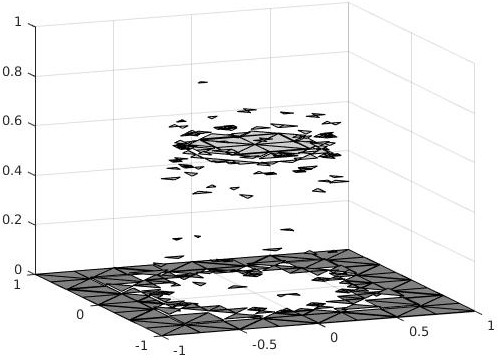
(a)

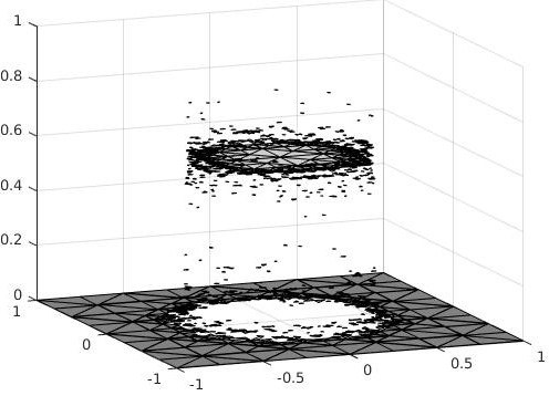
(b)

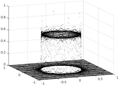
(c)

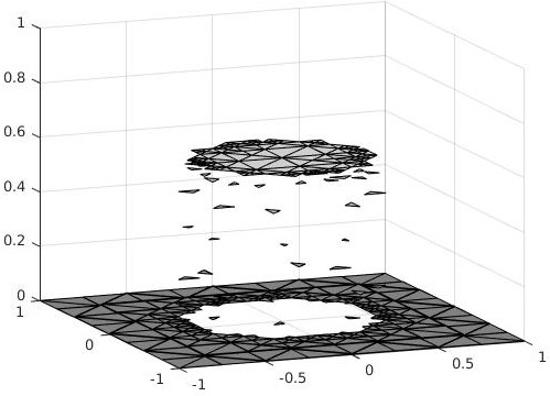
(d)

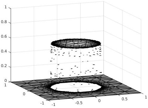
(e)

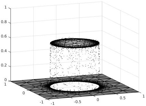
(f)

Figure 8. Piecewise constant approximations $\overline{u}_{h}=(1/\alpha)\operatorname{div}p_{h}+g_{h}$ for a sequence of adaptively refined triangulations for Example 6.2. Top: Dual variable is approximated in $Y_{h}^{C}=\mathcal{S}^{1}(\mathcal{T}_{h})^{d}$. Bottom: Dual variable is approximated in $Y_{h}^{dC}=\mathcal{L}^{1}(\mathcal{T}_{h})^{d}\cap H_{\rm N}(\operatorname{div};\Omega)$. One can observe oscillations of $\overline{u}_{h}$ along the jump set for the discretization of the dual ROF problem with $Y_{h}^{C}$.

In Figure 8 we depicted for a sequence of adaptively refined triangulations the piecewise constant approximations $\overline{u}_{h}=(1/\alpha)\operatorname{div}p_{h}+g_{h}$ with $p_{h}\in Y_{h}^{C}$ (top) and $p_{h}\in Y_{h}^{dC}$ (bottom), cf. Proposition 5.2. Although the different discretization methods for the dual problem do not affect the convergence rates in the presented experiments, the discretization of the dual problem with the continuous finite element space $Y_{h}^{C}$ causes oscillations in $\overline{u}_{h}$ along the jump set.

7. Conclusion

We have seen that the primal-dual gap error estimator defines a reliable upper bound with constant one for the error in the energy for convex minimization problems. For uniformly convex minimization problems it also controls the error with respect to a distance induced by the uniform convexity. The primal-dual gap error estimator has been introduced in [43] in an abstract setting and has been applied to several minimization problems in an infinite-dimensional framework. We extended the theory to general finite element discretizations of convex minimization problems and applied the theory to the nonlinear Laplace problem and the ROF problem, which serve as model problems for a wide class of convex minimization problems. The theoretical results, especially the reliability of the primal-dual gap error estimator, has been confirmed in several numerical experiments. In order to compute the estimator we approximately solved the primal and dual problems using the Variable-ADMM provided in [10]. Yet, it seems necessary to consider more efficient strategies to construct feasible functions especially for the dual problems.

References

- [1] M. Ainsworth and J. T. Oden. A posteriori error estimation in finite element analysis. Computer Methods in Applied Mechanics and Engineering, 142(1):1–88, 1997.
- [2] C. Atkinson and C. R. Champion. Some boundary-value problems for the equation . The Quarterly Journal of Mechanics and Applied Mathematics, 37(3):401–419, 1984.
- [3] C. Atkinson and C. W. Jones. Similarity solutions in some nonlinear diffusion problems and in boundary-layer flow of a pseudo plastic fluid. The Quarterly Journal of Mechanics and Applied Mathematics, 27:193–211, 1974.
- [4] G. Aubert and P. Kornprobst. Mathematical Problems in Image Processing, volume 147 of Applied Mathematical Sciences. Springer, 2nd edition, 2006.
- [5] I. Babuška and W. C. Rheinboldt. Error estimates for adaptive finite element computations. SIAM Journal on Numerical Analysis, 15(4):736–754, 1978.
- [6] Jacques Baranger and Khalid Najib. Numerical analysis of quasi-newtonian flow obeying the power low or the carreau flow. Numerische Mathematik, 58(1):35–49, 1990.
- [7] J. W. Barrett and W. B. Liu. Finite element approximation of the -Laplacian. Mathematics of Computation, 61(204):523–537, 1993.
- [8] S. Bartels. Error control and adaptivity for a variational model problem defined on functions of bounded variation. Mathematics of Computation, 84(293):1217–1240, 2015.
- [9] S. Bartels. Numerical Methods for Nonlinear Partial Differential Equations, volume 47 of Springer Series in Computational Mathematics. Springer, 2015.
- [10] S. Bartels and M. Milicevic. Alternating direction method of multipliers with variable step sizes. arXiv:1704.06069, 2017.
- [11] S. Bartels, R. H. Nochetto, and A. J. Salgado. Discrete total variation flows without regularization. SIAM Journal on Numerical Analysis, 52(1):363–385, 2014.
- [12] S. Bartels and P. Schön. Adaptive approximation of the monge-kantorovich problem via primal-dual gap estimates. ESAIM: M2AN, 51(6):2237–2261, 2017.
- [13] L. Belenki, L. Diening, and C. Kreuzer. Optimality of an adaptive finite element method for the -laplacian equation. IMA Journal of Numerical Analysis, 32:484–510, 2012.
- [14] D. Boffi, F. Brezzi, and M. Fortin. Mixed Finite Element Methods and Applications, volume 44 of Springer Series in Computational Mathematics. Springer, 2013.
- [15] S. C Brenner and L. R. Scott. The Mathematical Theory of Finite Element Methods, volume 15 of Texts in Applied Mathematics. Springer, 3rd edition, 2008.
- [16] C. Carstensen and R. Klose. A posteriori finite element error control for the -Laplace problem. SIAM Journal on Scientific Computing, 25(3):792–814, 2003.
- [17] C. Carstensen, W. B. Liu, and N. N. Yan. A posteriori fe error control for -Laplacian by gradient recovery in quasi-norm. Mathematics of Computation, 75(256):1599–1616, 2006.
- [18] S.-S. Chow. Finite element error estimates for non-linear elliptic equations of monotone type. Numerische Mathematik, 54(4):373–393, 1989.
- [19] L. Diening and C. Kreuzer. Linear convergence of an adaptive finite element method for the -Laplacian equation. SIAM Journal on Numerical Analysis, 46(2):614–638, 2008.
- [20] L. Diening and M. Růžička. Interpolation operators in orlicz–sobolev spaces. Numerische Mathematik, 107(1):107–129, 2007.
- [21] C. Ebmeyer. Mixed boundary value problems for nonlinear elliptic systems with ‐structure in polyhedral domains. Mathematische Nachrichten, 236(1):91–108.
- [22] C. Ebmeyer. Nonlinear elliptic problems with -structure under mixed boundary value conditions in polyhedral domains. Adv. Differential Equations, 6(7):873–895, 2001.
- [23] C. Ebmeyer. Global regularity in Sobolev spaces for elliptic problems with -structure on bounded domains. In J. F. Rodrigues, G. Seregin, and J. M. Urbano, editors, Trends in Partial Differential Equations of Mathematical Physics, pages 81–89, Basel, 2005. Birkhäuser Basel.
- [24] C. Ebmeyer and W. B. Liu. Quasi-norm interpolation error estimates for the piecewise linear finite element approximation of -Laplacian problems. Numerische Mathematik, 100(2):233–258, 2005.
- [25] C. Ebmeyer, W. B. Liu, and M. Steinhauer. Global regularity in fractional order sobolev spaces for the -Laplace equation on polyhedral domains. Z. Anal. Anwend., 24(2):353–374, 2005.
- [26] I. Ekeland and R. Témam. Convex Analysis and Variational Problems. Society for Industrial and Applied Mathematics, 1999.
- [27] L. El Alaoui, A. Ern, and M. Vohralík. Guaranteed and robust a posteriori error estimates and balancing discretization and linearization errors for monotone nonlinear problems. Computer Methods in Applied Mechanics and Engineering, 200(37):2782–2795, 2011. Special Issue on Modeling Error Estimation and Adaptive Modeling.
- [28] A. Ern and M. Vohralík. Adaptive inexact newton methods with a posteriori stopping criteria for nonlinear diffusion pdes. SIAM Journal on Scientific Computing, 35(4):A1761–A1791, 2013.
- [29] D. Gabay and B. Mercier. A dual algorithm for the solution of nonlinear variational problems via finite element approximation. Computers & Mathematics with Applications, 2(1):17–40, 1976.
- [30] R. Glowinski and A. Marroco. Sur l’approximation, par éléments finis d’ordre un, et la résolution, par pénalisation-dualité d’une classe de problèmes de Dirichlet non linéaires. R.A.I.R.O. Analyse Numérique, 9(R2):41–76, 1975.
- [31] K. Kunisch and M. Hintermüller. Total bounded variation regularization as a bilaterally constrained optimization problem. SIAM Journal on Applied Mathematics, 64(4):1311–1333, 2004.
- [32] W. B. Liu and J. W. Barrett. A further remark on the regularity of the solutions of the -Laplacian and its applications to their finite element approximation. Nonlinear Analysis: Theory, Methods & Applications, 21(5):379–387, 1993.
- [33] W. B. Liu and J. W. Barrett. A remark on the regularity of the solutions of the -Laplacian and its application to their finite element approximation. Journal of Mathematical Analysis and Applications, 178(2):470–487, 1993.
- [34] W. B. Liu and N. N. Yan. Quasi-norm a priori and a posteriori error estimates for the nonconforming approximation of -Laplacian. Numerische Mathematik, 89(2):341–378, 2001.
- [35] W. B. Liu and N. N. Yan. Quasi-norm local error estimators for -Laplacian. SIAM Journal on Numerical Analysis, 39(1):100–127, 2001.
- [36] W. B. Liu and N. N. Yan. On quasi-norm interpolation error estimation and a posteriori error estimates for -Laplacian. SIAM Journal on Numerical Analysis, 40(5):1870–1895, 2002.
- [37] M. Milicevic. Finite Element Discretization and Iterative Solution of Total Variation Regularized Minimization Problems and Application to the Simulation of Rate-Independent Damage Evolutions. PhD thesis, Albert-Ludwigs-Universität Freiburg, 2019.
- [38] R. H. Nochetto, K. G. Siebert, and A. Veeser. Theory of adaptive finite element methods: An introduction. In R. DeVore and A. Kunoth, editors, Multiscale, Nonlinear and Adaptive Approximation, pages 409–542, Berlin, Heidelberg, 2009. Springer Berlin Heidelberg.
- [39] J. R. Philip. -diffusion. Australian Journal of Physics, 14:1–13, 1961.
- [40] S. I. Repin. A posteriori error estimates for approximate solutions to variational problems with strongly convex functionals. Journal of Mathematical Sciences, 97(4):4311–4328, 1999.
- [41] S. I. Repin. A posteriori error estimates for approximate solutions of variational problems with functionals of power growth. Journal of Mathematical Sciences, 101(5):3531–3538, 2000.
- [42] S. I. Repin. A posteriori error estimation for nonlinear variational problems by duality theory. Journal of Mathematical Sciences, 99(1):927–935, 2000.
- [43] S. I. Repin. A posteriori error estimation for variational problems with uniformly convex functionals. Mathematics of Computation, 69(230):481–500, 2000.
- [44] S. I. Repin and L. S. Xanthis. A posteriori error estimation for elasto-plastic problems based on duality theory. Computer Methods in Applied Mechanics and Engineering, 138(1):317–339, 1996.
- [45] S. I. Repin and L. S. Xanthis. A posteriori error estimation for nonlinear variational problems. Comptes Rendus de l’Académie des Sciences - Series I - Mathematics, 324(10):1169–1174, 1997.
- [46] L. I. Rudin, S. Osher, and E. Fatemi. Nonlinear total variation based noise removal algorithms. Physica D: Nonlinear Phenomena, 60(1):259–268, 1992.
- [47] R. Stevenson. Optimality of a standard adaptive finite element method. Foundations of Computational Mathematics, 7(2):245–269, 2007.
- [48] M. Thomas. Quasistatic damage evolution with spatial -regularization. Discrete & Continuous Dynamical Systems - S, 6(1):235–255, 2013.
- [49] A. Veeser. Convergent adaptive finite elements for the nonlinear Laplacian. Numerische Mathematik, 92(4):743–770, 2002.
- [50] R. Verfürth. A Posteriori Error Estimation Techniques for Finite Element Methods. Oxford University Press, 2013.