Transient response of an electrolyte to a thermal quench

Abstract

We study the transient response of an electrolytic cell subject to a small, suddenly applied temperature increase at one of its two bounding electrode surfaces. An inhomogeneous temperature profile then develops, causing, via the Soret effect, ionic rearrangements towards a state of polarized ionic charge density $q$ and local salt density $c$. For the case of equal cationic and anionic diffusivities, we derive analytical approximations to $q,c$, and the thermovoltage $V_{T}$ for early ($t\ll\tau_{T}$) and late ($t\gg\tau_{T}$) times as compared to the relaxation time $\tau_{T}$ of the temperature. We challenge the conventional wisdom that the typically large Lewis number, the ratio $a/D$ of thermal to ionic diffusivities, of most liquids implies a quickly reached steady-state temperature profile onto which ions relax slowly. Though true for the evolution of $c$, it turns out that $q$ (and $V_{T}$) can respond much faster. Particularly when the cell is much bigger than the Debye length, a significant portion of the transient response of the cell falls in the $t\ll\tau_{T}$ regime, for which our approximated $q$ (corroborated by numerics) exhibits a density wave that has not been discussed before in this context. For electrolytes with unequal ionic diffusivities, $V_{T}$ exhibits a two-step relaxation process, in agreement with experimental data of Bonetti et al. [J. Chem. Phys. 142, 244708 (2015)].

I Introduction

The well-known Soret effect refers to the phenomenon that ions dissolved in a nonisothermal fluid can show preferential movement along or against thermal gradients, characterized by their heats of transport Agar et al. (1989); Würger (2010). Determining these ionic heats of transport, both experimentally Costesèque et al. (2004); Bonetti et al. (2011) and numerically Römer et al. (2013); Di Lecce et al. (2017); Di Lecce and Bresme (2018) is of primary importance for all applications involving nonisothermal electrolyte solutions, e.g., in colloid and polymer science. When ionic thermodiffusion is impeded, for instance, by blocking electrodes, local accumulations of either ionic species can be generated. Since such accumulations are not necessarily charge neutral, applying a temperature difference across an electrolyte can generate a so-called thermovoltage $V_{T}$. This thermovoltage, the ionic analog of the Seebeck potential in semiconductors, opens the door to energy scavenging from temperature differences Abraham et al. (2013); Zhao et al. (2016); Al-zubaidi et al. (2017); Liu et al. (2018). Since an electric current in an external circuit is only present during the transient build-up of $V_{T}(t)$ Wang et al. (2017), it is of interest to study how electrolytic cells respond shortly after a temperature difference is imposed. Bonetti et al. Bonetti et al. (2015) experimentally found that, after a seemingly instantaneous rise, $V_{T}(t)$ develops with the “slow” diffusion timescale $L^{2}/D_{+}$, with $2L$ being the electrode separation and $D_{+}$ the cationic diffusion constant.

Theoretical models were developed by Agar and Turner Agar and Turner (1960) and later by Stout and Khair Stout and Khair (2017), who both considered electrolytes with equal cationic and anionic diffusivities, $D_{+}=D_{-}\equiv D$. Motivated by the typically large ratio ${a}/D\approx 100$, with $a$ being the thermal diffusivity, their analyses departed from the ansatz that the steady-state temperature profile develops instantaneously [$T(x,t)=T(x)$, with $x$ being the spatial coordinate of their one-dimensional model electrolytic cells], after which ions relax slowly. With this ansatz, an exact expression for the transient response of the neutral salt density $c(x,t)$ Agar and Turner (1960) and approximate expressions for the ionic charge density $q(x,t)$ and corresponding $V_{T}(t)$ Stout and Khair (2017) were found. As we show in the present article, the corresponding exact solutions to $q$ and $V_{T}$ decay at late times with a common timescale $\tau_{q}=L^{2}/(D[(\kappa L)^{2}+\pi^{2}/4])$, with $\kappa$ being the inverse Debye length. This timescale and particularly the appearance of $\kappa$ therein presents us with two major problems. The first problem is that $\tau_{q}\approx 1/(D\kappa^{2})$ for large systems ($\kappa L\gg 1$), which does not explain the experimental observations of Ref. Bonetti et al. (2015) who found that $V_{T}$ develops much slower. As we show in this article, this discrepancy does not arise when one accounts for unequal diffusivities among ions. The second, conceptual, problem that $\tau_{q}$ hints at is that the ansatz $T(x,t)=T(x)$ can be unjustified. To see this, consider the ratio of the timescales of the pure thermal relaxation of the cell in the absence of ions [timescale $\tau_{T}=4L^{2}/(\pi^{2}{a})$, c.f. Eq. (III.1)] to that of the ionic charge relaxation:

$$\frac{\tau_{T}}{\tau_{q}}=\frac{D}{{a}}\left[1+\frac{4(\kappa L)^{2}}{\pi^{2}}\right]\,.$$ (1)

Since $\kappa$ depends on the salt concentration, this ratio can be varied over many decades, and is by no means restricted to $\tau_{T}/\tau_{q}\ll 1$ (requiring minute devices and very low salt concentrations). Hence, an instantaneous steady-state temperature profile onto which ions rearrange slowly is a special case of a more general problem. Given the longstanding experimental and theoretical interest in thermodiffusion of electrolytes Agar and Turner (1960); Stout and Khair (2017); Costesèque et al. (2004); Bonetti et al. (2015); Römer et al. (2013); Di Lecce et al. (2017); Di Lecce and Bresme (2018); Bonetti et al. (2011); Abraham et al. (2013), it is timely to discuss its solution.

II Setup

We consider an electrolytic cell (see Fig. 1) with two parallel flat electrodes at $x=\pm L$.

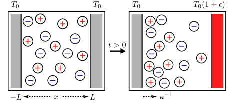
Figure 1: A model thermoelectric cell consisting of a 1:1 electrolyte with Debye length $\kappa^{-1}$ (solvent not shown) and two flat electrodes separated over a distance $2L$. At time $t=0$, the temperature of one electrode increases by a factor $1+\epsilon$.

Provided that the electrodes are much larger than their separation, we can ignore edge effects and treat this system as being one-dimensional. The electrodes are chemically inert and impermeable to ions and they are not connected by an external circuit, hence, do not acquire a surface charge. The cell is filled with an electrolyte solution at bulk salt concentration $\rho_{s}$ in a solvent of dielectric constant $\varepsilon$. The valence $z_{i}$ of ionic species $i=\{+,-\}$ is $z_{+}=1$ for the cations and $z_{-}=-1$ for the anions, respectively. The electrolyte is further characterized by ionic diffusion constants $D_{i}$, single-ion heats of transport $Q^{*}_{i}$, the mass density $\varrho$ (kg m^-3), the specific heat capacity $c_{p}$ (J K^-1 kg^-1), and the thermal conductivity $\kappa_{\theta}$ (J s^-1 m^-1 K^-1). For simplicity, we ignore all (salt) density dependence of these parameters. Moreover, we ignore convection here, which is reasonable if temperature differences are small and if the thermal gradient is aligned in the direction opposite to gravity Kalaydin et al. (2017). Alternatively, convection can be minimized in “microgravity,” e.g., onboard the International Space Station Triller et al. (2018).

II.1 Governing equations

The electrostatic potential $\psi(x,t)$, the local ionic number densities $\rho_{\pm}(x,t)$, and the local temperature $T(x,t)$ are modeled via the classical Poisson-Nernst-Planck and heat equations,

$$\varepsilon_{0}\varepsilon\partial^{2}_{x}\psi =-eq\,,$$ (2a)

$$\partial_{t}\rho_{i} =-\partial_{x}J_{i}\,,$$ (2b)

$$J_{i} =-D_{i}\left(\partial_{x}\rho_{i}+\frac{z_{i}e\rho_{i}}{k_{\rm B}T}\partial_{x}\psi+\frac{\rho_{i}Q^{*}_{i}}{k_{\rm B}T^{2}}\partial_{x}T\right)\,,$$ (2c)

$$\partial_{t}T ={a}\partial_{x}^{2}T-\frac{e}{\varrho c_{p}}(J_{+}-J_{-})\partial_{x}\psi\,,$$ (2d)

with $e$ being the proton charge and $\varepsilon_{0}$ being the vacuum permittivity. First, in the Poisson equation [(2a)] appears the ionic unit charge density $q=\rho_{+}-\rho_{-}$. Next, the Nernst-Planck equations [(2c)] account for diffusion, electromigration, and thermodiffusion. Finally, in the heat equation [(2d)] appears ${a}=\kappa_{\theta}/(\varrho c_{p})$, the thermal diffusivity, and a heat source term that was discussed at length in Refs. Janssen and van Roij (2017); Janssen et al. (2017).

Initially, the ionic density profiles and temperature are homogeneous:

$$\rho_{i}(x,t<0) =\rho_{s}\,, T(x,t<0) =T_{0}\,.$$ (3)

Thereafter, at $t=0$, the temperature of the electrode at $x=L$ is suddenly increased to $T(L,t=0)=T_{0}+\Delta T$, with $\Delta T>0$. For $t\geq 0$, the boundary conditions at the charge-neutral, ion-impermeable electrodes read

$$\partial_{x}\psi(\pm L,t) =0\,, J_{i}(\pm L,t) =0\,,$$ (4a)

$$T(-L,t) =T_{0}\,, T(L,t) =T_{0}+\Delta T\,.$$ (4b)

We note that Eq. (4a) only fixes $\psi$ up to a constant. Without loss of generality, we therefore moreover impose

$$\psi(L,t)=0\,.$$ (5)

This means that the thermovoltage, $V_{T}(t)=\psi(-L,t)-\psi(L,t)$, a key observable of our model system, simply reads $V_{T}(t)=\psi(-L,t)$.

II.2 Dimensionless formulation

We nondimensionalize Eqs. (2)-(5) with $\tilde{\psi}=\beta_{0}e\psi$ [with $\beta_{0}=1/(k_{\rm B}T_{0})$], $\tilde{T}=T/T_{0}$, $\tilde{x}=x/L$, $\tilde{t}=tD_{+}/L^{2}$, $\tilde{\rho}_{i}=\rho_{i}/\rho_{s}$, $\tilde{q}=q/\rho_{s}$, $\tilde{J}_{i}=J_{i}L/(D_{+}\rho_{s})$, and $\tilde{J}_{q}=\tilde{J}_{+}-\tilde{J}_{-}$ to find

$$2\partial_{\tilde{x}}^{2}\tilde{\psi} =-n^{2}\tilde{q},$$ (6a)

$$\partial_{\tilde{t}}\tilde{\rho}_{+} =\partial_{\tilde{x}}\left(\partial_{\tilde{x}}\tilde{\rho}_{+}+\frac{\tilde{\rho}_{+}}{\tilde{T}}\partial_{\tilde{x}}\tilde{\psi}+2\alpha_{+}\tilde{\rho}_{+}\partial_{\tilde{x}}\ln\tilde{T}\right)\,,$$ (6b)

$$\xi\partial_{\tilde{t}}\tilde{\rho}_{-} =\partial_{\tilde{x}}\left(\partial_{\tilde{x}}\tilde{\rho}_{-}-\frac{\tilde{\rho}_{-}}{\tilde{T}}\partial_{\tilde{x}}\tilde{\psi}+2\alpha_{-}\tilde{\rho}_{-}\partial_{\tilde{x}}\ln\tilde{T}\right)\,,$$ (6c)

$$\partial_{\tilde{t}}\tilde{T} =\frac{{a}}{D_{+}}\partial_{\tilde{x}}^{2}\tilde{T}-f\tilde{J}_{q}\partial_{\tilde{x}}\tilde{\psi}\,,$$ (6d)

and

$$\tilde{\rho}_{i}(\tilde{x},\tilde{t}<0) =1\,, \tilde{T}(\tilde{x},\tilde{t}<0) =1\,,$$ (7a)

$$\partial_{\tilde{x}}\tilde{\psi}(\pm 1,\tilde{t}\,) =0\,, \tilde{J}_{i}(\pm 1,\tilde{t}\,) =0\,,$$ (7b)

$$\tilde{T}(-1,\tilde{t}\geq 0) =1\,, \quad\tilde{T}(1,\tilde{t}\geq 0) =1+\epsilon\,,$$ (7c)

$$\tilde{\psi}(1,\tilde{t}\,) =0\,,$$ (7d)

where $\xi=D_{+}/D_{-}$ represents the ratio of ionic diffusivities, $f=k_{\rm B}\rho_{s}/(\varrho c_{p})$ is the ionic heat source coupling, $\alpha_{i}=Q^{*}_{i}/(2k_{\rm B}T)$ are the reduced Soret coefficients, and $\epsilon=\Delta T/T_{0}$ measures the size of the thermal quench. Moreover, $n=\kappa L$ is the dimensionless Debye separation parameter, with $\kappa^{-1}=[\varepsilon_{0}\varepsilon k_{\rm B}T_{0}/(2\rho_{s}e^{2})]^{1/2}$ being the Debye length. At steady state, $n$ measures to which extent nonzero $q$ values penetrate the bulk: While $n\gg 1$ indicates that $q$ is nonzero only in a small region close to the electrode surfaces, if $n\ll 1$, the ionic charge imbalance permeates the complete cell [cf. Eq. (15b)]. For reasons explained in Sec. III.2, we omitted $\partial_{\tilde{x}}D_{i}\partial_{\tilde{x}}\tilde{\rho}_{i}$ terms in Eqs. (6b) and (6c).

We see that our system is fully specified by seven dimensionless parameters, six of which ($n,\alpha_{\pm},\xi,{a}/D_{+}$, and $f$) appear in Eq. (6), and one of which ($\epsilon$) appears in Eq. (7c). In what follows, we will use the dimensionless formulation when we present simplifications to Eq. (6) because this simplifies calculations and because this highlights the roles played by these seven dimensionless parameters. However, when we present results, we prefer to restore to conventional units because that makes physical interpretation easier.

The next two sections [III and IV] deal with the case $\xi=1$, which is a reasonable simplification for several alkali halides. (For, e.g., KCl, RbBr, CsBr, and RbI, we find $\xi=0.97,1.00,1.00$, and $1.01$, respectively Agar et al. (1989)). We discuss the more general case of $\xi\neq 1$ in Sec. V. Importantly, we will find that the four quantities of our interest ($T$, $\psi$, $q$, and $c$) all relax at late times with one of three fundamental timescales: the “thermal diffusion time” $L^{2}/a$, the “diffusion time” $L^{2}/D$, or the “Debye time” $1/(D\kappa^{2})$.

III Analytical Approximations

We aim at deriving analytical approximations to Eqs. (6) and (7) for the case $\xi=1$. To do so, we employ an essential simplification of Eq. (6), namely, that $f\ll 1$ for most electrolytes. For small thermal quenches (cf. Sec. III.2) this means that the thermal problem [Eq. (6d)] decouples from the ionic problem [Eqs. (6a), (6b), and (6c)]. Accordingly, we first review the thermal relaxation of a pure solvent (Sec. III.1), which serves as input to determine $q,\psi$, and the local salt density $c=\rho_{+}+\rho_{-}$ (Secs. III.3 and III.4).

III.1 Pure thermal relaxation

In absence of ions, or when the source term of the heat equation is negligible, transient thermal response to a boundary value quench is governed by a simplified heat equation, $\partial_{t}T=a\partial_{x}^{2}T$, and the same initial and boundary conditions as in Eqs. (3) and (4b). Writing $\mathcal{K}_{j}=j\pi/2$ for $j=1,2,3,\dots$, the solution to this textbook problem reads Carslaw and Jaeger (1959); Cole et al. (2010)

$$\frac{T(x,t)-T_{0}}{\Delta T} =\sum_{j\geq 1}\frac{\sin[\mathcal{K}_{j}(x/L-1)]}{\mathcal{K}_{j}}\exp\!\left[-\mathcal{K}_{j}^{2}\frac{at}{L^{2}}\right]$$

$$\quad+\frac{1+x/L}{2}\,.$$ (8)

The infinite modes of $T$ decay at increasingly short timescales $L^{2}/(\mathcal{K}_{j}^{2}{a})$ with increasing $j$: the slowest mode ($j=1$) decays with $\tau_{T}\equiv 4L^{2}/(\pi^{2}{a})$, i.e., proportional to the thermal diffusion time.

At early times ($t\ll\tau_{T}$), $T(x,t)$ is barely affected by the Dirichlet boundary condition $T(-L,t)=T_{0}$. The temperature in the finite-sized cell can then also be modeled by the same heat equation in a semi-infinite geometry $x\in(-\infty,L]$. In that case we have Cole et al. (2010)

$$\frac{T(x,t)-T_{0}}{\Delta T} \approx\textrm{Erfc}\left[\frac{L-x}{2\sqrt{at}}\right]\,.$$ (9)

Naturally, the largest error made with this approximation occurs at the $x=-L$ boundary: $[T(-L,t)-T_{0}]/\Delta T=\textrm{Erfc}\left[L/\sqrt{at}\,\right]=\{2.1\times 10^{-45},7.8\times 10^{-6},0.16\}$ at $ta/L^{2}=\{10^{-2},10^{-1},1\}$, respectively. Hence, Eq. (9) can be safely used up to $ta/L^{2}=10^{-1}$.

III.2 Small-$\epsilon$ expansions

As we show next, for $\epsilon\ll 1$, we can analytically solve Eqs. (6a), (6b), and (6c) both at early times [using Eq. (9)] and at late times [using the steady-state limit of Eq. (III.1)]. To do so, we expand $\psi$, $q$, and $c$ in the small parameter $\epsilon$: $\psi=\psi_{0}+\epsilon\psi_{1}+\mathcal{O}(\epsilon^{2})$, $q=q_{0}+\epsilon q_{1}+\mathcal{O}(\epsilon^{2})$, and $c=c_{0}+\epsilon c_{1}+\mathcal{O}(\epsilon^{2})$, respectively, and do the same for the remaining five dimensionless parameters: $\alpha_{i}=\alpha_{i,0}+\epsilon\alpha_{i,1}+\mathcal{O}(\epsilon^{2})$, etc. Inserting those variables and parameters into Eqs. (6a), (6b), and (6c) results in $\mathcal{O}(1)$ problems that characterize the initial isothermal situation (clearly, $\psi_{0}=0$, $q_{0}=0$, and $c_{0}=2\rho_{s}$), and different $\mathcal{O}(\epsilon)$ problems for $\psi_{1},q_{1}$, and $c_{1}$ for the early- and late-time response. With a slight abuse of notation, from hereon, we drop the subscript zeros of all dimensionless parameters, because subscript-one parameters only appear in $\mathcal{O}(\epsilon^{2})$ terms. Likewise, if $a$ depends on $T$, Eqs. (III.1) and (9) apply only if $\epsilon\ll 1$. (When we presented these equations for arbitrary $\epsilon$, we tacitly assumed that $a(T)=a$). We moreover note that the source term in Eq. (2d) is $\mathcal{O}(\epsilon^{2})$. This means that the results of Sec. III.1, derived by setting $f=0$, are accurate for finite $f$ as well. Finally, we omitted $\partial_{\tilde{x}}D_{i}\partial_{\tilde{x}}\tilde{\rho}_{i}$ in Eqs. (6b) and (6c) because these terms are $O(\epsilon^{2})$ as well.

III.3 Early-time ($t\ll\tau_{T}$) ionic response

Inserting Eq. (9) into Eqs. (6b) and (6c) yields

$$\partial_{\tilde{t}}\tilde{q}_{1} =\partial^{2}_{\tilde{x}}\tilde{q}_{1}-n^{2}\tilde{q}_{1}+\frac{{\alpha_{\rm d}}(1-\tilde{x})}{\sqrt{\pi}(a\tilde{t}/D)^{3/2}}\exp{\bigg{[}-\frac{D(1-\tilde{x})^{2}}{4a\tilde{t}}\bigg{]}}$$ (10a)

$$\partial_{\tilde{t}}\tilde{c}_{1} =\partial^{2}_{\tilde{x}}\tilde{c}_{1}+\frac{{\alpha_{\rm s}}(1-\tilde{x})}{\sqrt{\pi}(a\tilde{t}/D)^{3/2}}\exp{\bigg{[}-\frac{D(1-\tilde{x})^{2}}{4a\tilde{t}}\bigg{]}}\,,$$ (10b)

with $\alpha_{\rm d}=\alpha_{+}-\alpha_{-}$ and $\alpha_{\rm s}=\alpha_{+}+\alpha_{-}$. The $n^{2}\tilde{q}_{1}$ term in Eq. (10a) stems from the electromotive term $2\partial^{2}_{\tilde{x}}\tilde{\psi}_{1}$ in $\tilde{J}_{q}$, together with Eq. (6a). The corresponding electromotive term in the salt flow $\partial_{\tilde{x}}[\tilde{q}_{1}\partial_{\tilde{x}}\tilde{\psi}_{1}]$ is $\mathcal{O}(\epsilon^{2})$ thus neglected in Eq. (10b).

At time $t=0$, the system is charge neutral [$q(x,t)=0$] and the nonzero ionic charge current is caused solely by thermodiffusion. There will be early (but finite) times at which thermodiffusion still dominates electromigration: times, thus, at which the electromotive term $n^{2}\tilde{q}_{1}$ in Eq. (10a) can be neglected. Clearly, (1) we cannot expect to find a self-consistent nonzero solution for $q(x,t)$ in this way and (2) the temporal range of validity of this approximation will decrease with increasing $n$. With the omission of the $n^{2}\tilde{q}_{1}$ term in Eq. (10a), the equations governing the early-time response of $\tilde{q}_{1}/\alpha_{d}$ and $\tilde{c}_{1}/\alpha_{\rm s}$ are the same. Since the same equations have the same solutions, our forthcoming results for $q_{1}$ are trivially transferable to $c_{1}$. Substituting $p=D(\tilde{x}-1)^{2}/(4a\tilde{t}\,)$ in Eq. (10a) yields a inhomogeneous ordinary differential equation:

$$p\frac{\mathrm{d}^{2}\tilde{q}_{1}}{\mathrm{d}p^{2}}+\left(\frac{1}{2}+p\frac{a}{D}\right)\frac{\mathrm{d}\tilde{q}_{1}}{\mathrm{d}p} =-\frac{2{\alpha_{d}}}{\sqrt{\pi}}\sqrt{p}\exp{[-p]}\,,$$ (11a)

$$\sqrt{p}\frac{\mathrm{d}\tilde{q}_{1}}{\mathrm{d}p}\bigg{|}_{p=0} =\frac{2{\alpha_{d}}}{\sqrt{\pi}}\,,$$ (11b)

where Eq. (11b) follows from $\tilde{J}_{q}(1,\tilde{t}\,)=0$ [cf. Eq. (7b)]. While Eq. (11b) fixes one of the two integration constants of the general solution of Eq. (11a), it turns out that the other integration constant cannot be fixed by $\tilde{J}_{q}(\tilde{x}=-1,t)=0$; we simply do not have the freedom to impose $\mathrm{d}\tilde{q}_{1}/\mathrm{d}p$ in two positions. This must be because Eq. (11a) resulted from a procedure that ignores the electrode at $\tilde{x}=-1$. To fix this second integration constant nevertheless, we enforce charge neutrality $\int_{-1}^{1}\mathrm{d}\tilde{x}\,\tilde{q}_{1}(\tilde{x},\tilde{t}\,)=0\Rightarrow\int_{0}^{D/(a\tilde{t}\,)}\mathrm{d}p\,\tilde{q}_{1}(p)/\sqrt{p}=0$, which arises naturally from Eqs. (2b) and (4a). We find

$$\frac{q_{1}(x,t)}{2\rho_{s}\alpha_{d}} =\frac{2D}{D-a}\Bigg{\{}\frac{\sqrt{at}}{L\sqrt{\pi}}\left(\exp\left[-\frac{L^{2}}{Dt}\right]-\exp\left[-\frac{L^{2}}{at}\right]\right)$$

$$\quad\quad\,\,\,-\sqrt{\frac{{a}}{{D}}}\textrm{Erf}\left[\frac{L-x}{2\sqrt{Dt}}\right]+\textrm{Erf}\left[\frac{L-x}{2\sqrt{at}}\right]$$

$$\quad\quad\,\,+\sqrt{\frac{{a}}{{D}}}\textrm{Erf}\left[\frac{L}{\sqrt{Dt}}\right]-\textrm{Erf}\left[\frac{L}{\sqrt{at}}\right]\Bigg{\}}\,,$$ (12)

and the same for $c_{1}/(2\rho_{s}\alpha_{s})$.

We can now find $\psi(x,t)$ by integrating $q_{1}$ twice and enforcing $\psi(L,t)=0$ and $\partial_{x}\psi(L,t)=0$. The solution, which is too lengthy to be reproduced here, turns out to satisfy the boundary condition $\partial_{x}\psi(-L,t)=0$ as well. This means that the electromotive term drops out of $\tilde{J}_{q}(-1,\tilde{t})$. We determined the importance of the two remaining terms in $\tilde{J}_{q}(-1,\tilde{t})=-\partial_{\tilde{x}}\tilde{q}_{1}(-1,\tilde{t})-2\alpha_{d}\partial_{\tilde{x}}\ln\tilde{T}(-1,\tilde{t})$ with Eqs. (9) and (III.3) and found for $a/D=100$ that $\tilde{J}_{q}(-1,\tilde{t})=\{10^{-43},1.8\times 10^{-4}\}$ at $ta/L^{2}=\{10^{-1},1\}$, respectively. Hence, as long as Eq. (9) approximates $T(x,t)$ decently, the boundary condition $\tilde{J}_{q}(-1,\tilde{t}\,)=0$ that we could not strictly impose is satisfied approximately nevertheless.

III.4 Late-time ($t\gg\tau_{T}$) ionic response

Upon inserting the steady-state temperature profile $\tilde{T}=1+\epsilon(1+\tilde{x})/2$, at $\mathcal{O}(\epsilon)$, Eqs. (6b) and (6b) give rise to

$$\partial_{\tilde{t}}\tilde{q}_{1} =\partial^{2}_{\tilde{x}}\tilde{q}_{1}-n^{2}\tilde{q}_{1}\,, \quad\quad\quad\partial_{\tilde{t}}\tilde{c}_{1} =\partial^{2}_{\tilde{x}}\tilde{c}_{1}\,.$$ (13)

Here, the thermodiffusion terms in the ionic fluxes amount to constants $\tilde{J}_{i}\sim\epsilon\alpha_{i}$; hence, their spatial derivatives are absent in Eq. (13). As pointed out by Refs. Costesèque et al. (2004); Stout and Khair (2017), $\alpha_{\rm s}$ and $\alpha_{\rm d}$ then only appear in the boundary conditions,

$$\tilde{q}_{1}(\tilde{x},\tilde{t}<0) =0\,, \tilde{c}_{1}(\tilde{x},\tilde{t}<0) =0\,,$$ (14a)

$$\partial_{\tilde{x}}\tilde{q}_{1}(\pm 1,\tilde{t}\,) =-\alpha_{\rm d}\,, \quad\partial_{\tilde{x}}\tilde{c}_{1}(\pm 1,\tilde{t}\,) =-\alpha_{\rm s}\,,$$ (14b)

hence do not affect the relaxation rates. Only few of the original seven dimensionless numbers controlling Eqs. (6) and (7) now remain. We set $\xi=1$ and, by using the steady-state temperature profile, we have effectively set ${a}/D\to\infty$. With these choices, $\alpha_{\pm}$ moved from the PDEs to the BCs. Moreover, as long as $f\lessapprox 1$, the source term of the heat equation (6d) is $\mathcal{O}(\epsilon^{2})$ hence irrelevant. With $\epsilon$ only appearing in the small-$\epsilon$ expansions, $n$ is the only remaining parameter that can influence the relaxation rates of our system. In Appendix A we solve Eqs. (6a) and (13) subject to Eq. (14). Writing $\mathcal{N}_{j}=(j-1/2)\pi$ for $j=1,2,3,\dots$, the solutions read

$$\frac{e\psi_{1}(x,t)}{k_{\rm B}T_{0}\alpha_{\rm d}} =-n^{2}\sum_{j\geq 1}\frac{1+(-1)^{j}\sin\!\left[\mathcal{N}_{j}x/L\right]}{\mathcal{N}_{j}^{2}\left[n^{2}+\mathcal{N}_{j}^{2}\right]}\exp{\left[-t/\tau_{q}^{j}\,\right]}$$

$$\quad+\frac{1}{2n}\frac{\sinh(nx/L)-\sinh n}{\cosh n}+\frac{1}{2}-\frac{x}{2L}\,,$$ (15a)

$$\frac{q_{1}(x,t)}{2\rho_{s}\alpha_{\rm d}} =-2\sum_{j\geq 1}\frac{(-1)^{j}\sin\!\left[\mathcal{N}_{j}x/L\right]}{n^{2}+\mathcal{N}_{j}^{2}}\exp{\left[-t/\tau_{q}^{j}\,\right]}$$

$$\quad-\frac{1}{n}\frac{\sinh(nx/L)}{\cosh n}\,,$$ (15b)

$$\frac{c_{1}(x,t)}{2\rho_{s}\alpha_{\rm s}} =-2\sum_{j\geq 1}\frac{(-1)^{j}\sin\!\left[\mathcal{N}_{j}x/L\right]}{\mathcal{N}_{j}^{2}}\exp{\left[-\frac{\mathcal{N}_{j}^{2}\,Dt}{L^{2}}\,\right]}$$

$$\quad-\frac{x}{L}\,,$$ (15c)

where $\tau_{q}^{j}=L^{2}/[D\left(n^{2}+\mathcal{N}_{j}^{2}\right)]$ and where Eq. (15c) appeared previously in Ref. Agar and Turner (1960). We see that, indeed, the relaxation of $\psi$ and $q$ (in units of $L^{2}/D$) depends only on $n$, while the relaxation of $c$ (in units of $L^{2}/D$) has no parametric dependence whatsoever. At late times, the relaxation of the functions in Eq. (15) is dominated by the $j=1$ terms of the sums: While $c$ decays with $4L^{2}/(\pi^{2}D)$, $\psi$ and $q$ relax with $\tau_{q}\equiv L^{2}/\left[D\left(n^{2}+\pi^{2}/4\right)\right]$, as anticipated in the introduction. Hence, for $n\ll 1$ we find a universal decay time $4L^{2}/(\pi^{2}D)$ proportional to the diffusion time, whereas for $n\gg 1$, $\psi$ and $q$ relax with the Debye time $1/(D\kappa^{2})$.

IV Results

We numerically solved Eq. (6) with comsol multiphysics 5.4 for $\xi=1$, ${a}/D=100$, $\alpha_{+}=0.5$, $\alpha_{-}=0.1$, $f=2\times 10^{-3}$, $\epsilon=10^{-3}$, and $n=1$ and $n=100$. This parameter set is representative for an aqueous KCl solution ($\varrho\approx 10^{6}$ g m^-3, $c_{p}\approx 4$ J g^-1, $a/D$, and $\alpha_{\pm}$ from Ref. Stout and Khair (2017)) subject to a thermal quench of $0.3$ K around room temperature. Because $\kappa^{-1}$ amounts to several tens of nanometers at most (at 1 mM, $\kappa^{-1}=9.6$ nm), large $n$ values can be easily achieved experimentally by using $L$ values in the micrometer regime (or larger). Conversely, the small $n=1$ value requires both high dilution and minute devices ($L$ in the nanometer regime). While this latter case might be difficult to reach experimentally, we discuss $n=1$ because, judging from Eq. (1), if anywhere, this is the parameter setting for which the instantaneous temperature ansatz [and Eq. (15)] should work best.

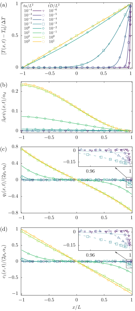
Figure 2: Thermal and ionic relaxation at $n=1$ and ${a}/D=100$ in response to a thermal quench ($\epsilon=10^{-3}$) at $x=L$. Numerical solution (symbols) to Eq. (6) at times $tD/L^{2}=\{10^{-6}-10\}$ for $T$ (a), $\psi$ (b), $q$ (c), and $c$ (d) where obtained at $\xi=1$, $\alpha_{+}=0.5$, $\alpha_{-}=0.1$, $f=2\times 10^{-3}$. (a) Also shows Eq. (III.1) (lines) at the same times and Eq. (9) (plusses) at $tD/L^{2}=10^{-3}$. (b)-(d) Also show Eq. (15) with lines. The insets of (c) and (d) show Eq. (III.3) (dashed lines) at times $tD/L^{2}=\{10^{-6}-10^{-3}\}$

IV.1 Local fields at $n=1$

We show analytical (lines) and numerical (symbols) solutions to Eq. (6) for $n=1$ in Fig. 2, where we plot the position dependence of $T$, $\psi$, $q$, and $c$ for logarithmically separated times between $tD/L^{2}=10^{-6}$ and $tD/L^{2}=10$. In Fig. 2 (a) we show the temperature. As a sanity check, we also compared numerical solutions for $(T(x,t)-T_{0})/\Delta T$ at $f=0$ to the exact result Eq. (III.1) [in this section we truncate the sums in Eqs. (III.1) and (15) after 2000 terms]: The difference between either predictions was at most $0.02$ (at $tD/L^{2}=10^{-6}$), dropping to $10^{-12}$ at late times. The difference between $T$ calculated with either $f=2\times 10^{-3}$ or $f=0$ (and other parameters as before) was too small to detect within this numerical error margin. In any case, with our choice $f=2\epsilon$, the source term of the heat equation (6d) is $\mathcal{O}(\epsilon^{3})$. Therefore, its effects are beyond the range of validity of our theory.

As anticipated in Sec. III.1, Fig. 2(a) moreover shows that Eq. (9) accurately describes $T(x,t)$ at $ta/L^{2}=0.1$ (plusses) as well as at earlier times (not shown). For the stated parameter set, Fig. 2 shows that $T(x,t)$ relaxes almost completely before $\psi,q$, and $c$ deviate from their initial values. Consequently, the ionic relaxation falls predominantly in the late-time regime ($t\gg\tau_{T}$) discussed in Sec. III.4: From $ta/L^{2}=10$ onwards, the assumption of a thermal steady state that we used to derive Eq. (15) is justified. Consequently, at late times, we observe a decent correspondence between numerics and the analytical predictions for $\psi_{1},q_{1}$, and $c_{1}$ [Eqs. (15a), (15b), and (15c), respectively]. Conversely, at early times ($t\ll\tau_{T}$), when Eq. (9) accurately describes $T(x,t)$, one expects the predictions of Eq. (III.3) for $q_{1}$ and $c_{1}$ to be accurate. Indeed, the inset of Fig. 2(c) (a zoom-in of the main panel to the region $x\lessapprox L$) shows an excellent agreement between Eq. (III.3) (dashed lines) and the same numerical data until $tD/L^{2}=10^{-3}$, while at that same time, Eq. (15b) gives erroneous predictions (the line does not pierce the open squares). Interestingly, this inset exhibits a tiny ionic charge density wave that moves with the front of thermal perturbation and that breaks the antisymmetry (present at late times) of $q$ and $c$ around the midplane at early times. Given the equivalence at early times of $q_{1}/\alpha_{d}$ to $c_{1}/\alpha_{s}$ as discussed in Sec. III.3, the inset of Fig. 2(d) shows that the same analytical expression Eq. (III.3) also describes the evolution of $c_{1}$ at early times well.

IV.2 Local fields at $n=100$

Figure 3 shows numerical solutions to Eq. (6) and the same analytical approximations as before, now for $n=100$.

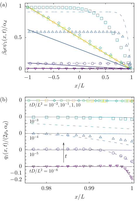
Figure 3: Numerical (symbols) and analytical (lines) results for $\psi_{1}$ (a) and $q_{1}(x,t)$ (b) at $n=100$. All other parameters, colors, symbols, and line styles are as in Fig. 2.

Since $T$ and $c_{1}$ are essentially $n$ independent [cf. Eqs. (III.1), (9), (III.3) and (15)], we only show $\psi_{1}$ in Fig. 3(a) and $q_{1}$ in Fig. 3(b). We see in Fig. 3(b) that Eq. (III.3) is now accurate only until $tD/L^{2}=10^{-5}$ [as this equation is $n$ independent, the dashed lines in Fig. 3(b) are the same as in the inset of Fig. 2(c)]. This difference with the $n=1$ case (accurate until $tD/L^{2}=10^{-3}$) is understood in terms of the larger error made for higher $n$ in neglecting the term $n^{2}\tilde{q}_{1}$ in Eq. (10a). Equation (15b) is accurate after $tD/L^{2}=10^{-2}$, comparable to $tD/L^{2}=10^{-1}$ for the $n=1$ case. The key difference with the $n=1$ case, however, is that at $tD/L^{2}=10^{-1}$, $q_{1}(x,t)$ has already reached its steady-state profile [cf. Eq. (1): With increasing $n$, the early-time ($t\ll\tau_{T}$) regime of the transient response of $q$ and $\psi$ gains in importance]. Hence, Eq. (15b) is irrelevant for the description of the transient behavior of $q(x,t)$ for $n=100$ and solely captures its steady state. Yet, out of curiosity, we plot the corresponding late-time expression for $\psi_{1}$ [Eq. (15a)] in Fig. 3(a); while this expression gets the shape of $\psi_{1}$ completely wrong (except at steady state), it surprisingly accurately estimates the thermovoltage $V_{T}(t)=\epsilon\psi_{1}(-L,t)+\mathcal{O}(\epsilon^{2})$ at all times considered. Apparently, for the development of $V_{T}(t)$, it is not necessary that the thermal perturbation has spanned the system: The local charge separation as observed in Fig. 3(b) leads to the same voltage drop, but now already over the small region coincident with the thermal perturbation. Meanwhile, it comes as somewhat of a surprise that the analytical prediction for $\psi_{1}$ calculated with Eqs. (III.3) provides fair approximations to our numerical results only for very early times ($tD/L^{2}=10^{-6},10^{-5}$), thereafter overestimating $\psi_{1}$ greatly. Since this method to approximate $\psi_{1}$ already goes awry at $t\ll\tau_{T}$, discrepancies cannot be attributed to usage of the approximate early-time temperature [Eq. (9) instead of Eq. (III.1)] in the derivation of Eq. (III.3). Apparently, $\psi_{1}$ is very sensitive to the errors in $q_{1}$ (observable in Fig. 3(b) from $tD/L^{2}=10^{-4}$ onwards) resulting from the omission of the electromotive term $\tilde{c}_{0}\partial^{2}_{\tilde{x}}\tilde{\psi}_{1}$ in Eq. (10).

IV.3 Boundary value relaxation

In Fig. 4 we show numerics (symbols) and analytical predictions from Eq. (15) (lines) for the relaxation of $\psi_{1}(-L,t)$ and the absolute boundary values of the ionic charge and salt densities, $|q_{1}(\pm L,t)|$ and $|c_{1}=\pm L,t)|$, respectively. Concerning $V_{T}(t)=\epsilon\psi_{1}(-L,t)+\mathcal{O}(\epsilon^{2})$, we see that analytical predictions agree well with numerics for $n=1$ [unsurprising, given the agreement observed in Fig. 2(b)] and $n=100$, where a minor discrepancy is observed at very early times. Again, since the steady-state temperature ansatz is only justifiable after $tD/L^{2}=0.1$, the good agreement observed Fig. 4(b) between numerics and Eq. (15a) up to $tD/L^{2}=10^{-6}$ [pushing that equation five orders of magnitude into temporal terra incognita] is remarkable.

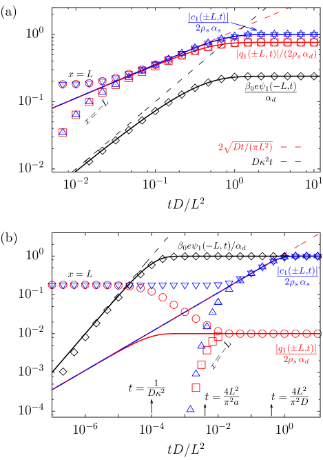
Figure 4: The relaxation of $\psi_{1}(-L,t),q_{1}(\pm L,t)$, and $c_{1}(\pm L,t)$ (black, red, blue) from numerics (symbols) and Eq. (15) (lines) ($j\leq 10$), for $n=1$ (a) and $n=100$ (b). Plotted as well are $D\kappa^{2}t$ (black dashed) and $2\sqrt{Dt/(L^{2}\pi)}$ (red dashed).

The small-$t$ scaling of $\beta_{0}eV_{T}/(\alpha_{d}\epsilon)=\kappa^{2}Dt$ (black dashed lines) is derived in Appendix B.

We see in Fig. 4 that, at early times ($t<\tau_{T}$), $|c_{1}(\pm L,t)|$ and $|q_{1}(\pm L,t)|$ are perturbed at the quenched ($x=L$) electrode (down triangles and circles), and unperturbed at the other side (up triangles and squares). With Eq. (III.3) we find that the early-time plateaus observed in Fig. 4 lie at $\lim_{t\to 0^{+}}|q_{1}(L,t)|/(2\rho_{s}\alpha_{d})=\lim_{t\to 0^{+}}|c_{1}(L,t)|/(2\rho_{s}\alpha_{s})=2/(1+\sqrt{a/D})\approx 0.18$, independent of $n$. Interestingly, at $n=100$ this prediction for $c_{1}$ is still accurate around $t\approx\tau_{T}$, when Eq. (III.3) inaccurately describes $q_{1}$ [Fig. 3(b)]. At $n=1$ the omission of the $n^{2}q_{1}$ term in Eq. (10a) is justifiable and the prediction $\lim_{t\to 0^{+}}|q_{1}(L,t)|/(2\rho_{s}\alpha_{d})\approx 0.18$ holds up to $t\approx\tau_{T}$ as well. From $tD/L^{2}=0.01\Leftrightarrow t\approx\tau_{T}$ onwards, we see, for $n=1$, that numerics and analytical predictions from Eq. (15) converge, in line with our observations in Fig. 2. Once converged, they scale as $|q_{1}(\pm L)|=|c_{1}(\pm L)|=2\sqrt{Dt/(L^{2}\pi)}$ (red dashed lines) as derived in Appendix B, finally relaxing to their steady-state values around $tD/L^{2}=1\Leftrightarrow t\approx\tau_{q}$.

For $n=100$ and $a/D=100$, Eq. (15) predicts that $V_{T}(t)$ and $q_{1}(\pm L,t)$ relax two orders of magnitude faster [at $t=L^{2}/(D[n^{2}+\pi^{2}/4])\approx 1/(D\kappa^{2})$] than $T$ [at $t=4L^{2}/(a\pi^{2})$]. While $V_{T}(t)$ really does develop on this short timescale (as discussed above), $q_{1}(\pm L,t)$ becomes enslaved to the “slow” thermal relaxation. Together with relaxation of $c_{1}(\pm L,t)$ at $t=4L^{2}/(D\pi^{2})$, Fig. 4(b) shows a separation of timescales over four orders of magnitude for the three observables $\psi_{1}(-L,t),|q_{1}(\pm L,t)|$, and $|c_{1}(\pm L,t)|$. The separation of timescales of boundary observables $V_{T}(t)$ and $q(\pm L,t)$ seems to contradict the intuition that ionic charge and electrostatic potential are instantaneously related via the Poisson equation, and should thus relax in lockstep. However, the Poisson equation is a nonlocal relation between $\psi(x,t)$ and $q(x,t)$, which, apparently, does not forbid $\psi$ and $q$ to relax differently at specific locations. Indeed, Fig. 3(a) clearly shows that the overall electrostatic potential $\psi_{1}(x,t)$ reaches its steady state much later (around $ta/L^{2}=1$) than $\psi_{1}(-L,t)$.

V Unequal ionic diffusivities

We note that our finding $V_{T}(t)\sim\exp[-D\kappa^{2}t]$ in Fig. 4(b) is at odds with the experimental data of Ref. Bonetti et al. (2015). They studied a $6$-mm-wide cell filled with a concentrated electrolyte (2M EMIMTFSI in acetonitrile) subject to a thermal quench of $\Delta T=20$ K. Their measurements indicated that $V_{T}(t)\sim\exp[-\pi^{2}D_{+}t/(4L^{2})]$, where the fitted cationic diffusion constant $D_{+}$ was a factor 3 off from literature values for the pure EMIMTFSI ionic liquid (without solvent). In principle, the discrepancy between our works could have arisen due to several simplifying assumptions underlying our model, as their setup: (1) used a concentrated electrolyte, for which our continuum Nernst-Planck description of the ionic currents (reasonable for dilute electrolytes) might be unsuitable and to which it is difficult to assign a Debye length; (2) had comparable lateral and in-plane dimensions, which further undermines our one-dimensional model; and (3) was exposed to a thermal quench two orders of magnitude larger than what we imposed in Sec. IV. Accordingly, we performed exploratory numerical simulations of Eq. (6) with $\epsilon=0.1$ (and $T$ independent dimensionless parameters) and found that the third speculation does not explain the discrepancy: In that case, the qualitative behavior [including the fast $V_{T}(t)\sim\exp[-D\kappa^{2}t]$-relaxation] of our model is unaltered, with the notable exception that the antisymmetry of the steady-state profiles of $c$ and $q$ around $x=0$ is broken.

Instead of the above three speculations, it turns out that the qualitative features of the experimental data of Ref. Bonetti et al. (2015) can be reproduced by our model if one accounts for different diffusivities among the ions private . After all, NMR measurements of pure EMIMTFSI (without solvent) determined an apparent cationic transference number $D_{+}/(D_{-}+D_{+})\approx 0.63$, which implies $\xi=1.7$ Noda et al. (2001).

Once more using the steady-state temperature ansatz, in Appendix C we derive $V_{T}$ for $n\gg 1$ and for general $\xi$:

$$\frac{eV_{T}(t)}{k_{\rm B}T_{0}\epsilon} =\alpha_{\rm d}-2\alpha_{\rm s}\frac{1-\xi}{1+\xi}\sum_{j\geq 1}\frac{1}{\mathcal{N}_{j}^{2}}\exp{\left[-\frac{2\mathcal{N}_{j}^{2}}{1+\xi}\frac{D_{+}t}{L^{2}}\right]}-4\frac{\xi\alpha_{+}-\alpha_{-}}{1+\xi}\sum_{j\geq 1}\frac{1}{\mathcal{N}_{j}^{2}}\exp{\left[-\frac{1+\xi}{2\xi}D_{+}\kappa^{2}t\right]}+\mathcal{O}\left(n^{-1}\right)+\mathcal{O}\left(\epsilon\right)\,,$$ (16)

which reduces correctly to the $n\gg 1$ limit of $\psi_{1}(-L)$ [cf. Eq. (B)] for $\xi=1$. Strikingly, in Eq. (16) now appear relaxation times that scale like the diffusion time as $\sim L^{2}$, which is a promising sign for our attempt at explaining the data of Ref. Bonetti et al. (2015). Moreover, we can rewrite the exponents of Eq. (16) to $\exp{\left[-D_{a}\kappa^{2}t\right]}$ and $\exp{\left[-\mathcal{N}_{j}^{2}D_{h}t/L^{2}\right]}$, respectively, with $D_{a}\equiv(D_{-}+D_{+})/2$ being the arithmetic and $D_{h}\equiv 2/[(1/D_{-}+1/D_{+})]$ being the harmonic mean of the ionic diffusion constants, respectively Alexe-Ionescu et al. (2007); Balu and Khair (2018). Notably, precisely these two means appear in the electrolyte conductance and in Nernst’s expression for the ambipolar diffusivity of neutral salt, respectively. While it is now tempting to interpret $V_{T}(t)$ as being generated simultaneously by ionic charge density and salt density relaxation, we note that $V_{T}(t)$ is ultimately only directly related to $q(x,t)$ (cf. Appendix C). The appearance of parameters typical for salt diffusion ($\alpha_{s}$ and $L^{2}/D_{h}$) merely suggests that there is a nontrivial coupling between $c$ and $q$ whenever $\xi\neq 1$. We leave an in-depth analysis of $q$ and $c$ at $\xi\neq 1$ for future work.

In Fig. 5, we plot Eq. (16) (lines) for $n=100$ and several $\xi=\{10,5,2,1,0.5,0.2,0.1\}$, and all other parameters the same as in Sec. IV.

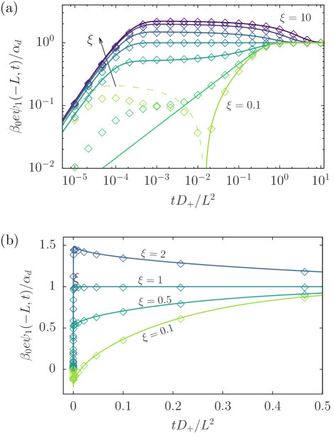
Figure 5: Predictions for $V_{T}(t)=\epsilon\psi_{1}(-L,t)+\mathcal{O}(\epsilon^{2})$ from a numerical simulation of Eq. (6) (symbols) and from the analytical expression Eq. (16) (lines), on double logarithmic scales (a) and linear scales (b). The dashed line represents $-\psi_{1}(-L,t)$ at times where $\psi_{1}(-L,t)<0$. In (a), going from top to bottom, the lines represent $\xi=\{10,5,2,1,0.5,0.2,0.1\}$. All other parameters are the same as in Fig. 2.

Overall, we observe a good agreement between that equation and numerical simulations of Eq. (6) (symbols). Noticeable deviations occur for small $\xi$ and $t<\tau_{T}$, when the steady-state temperature ansatz used to derive Eq. (16) is unjustified. Note, also, that the $\xi=1$-case corresponds to the black diamonds in Fig. 4(b). For $\xi\neq 1$, the data plotted on double logarithmic scales [Fig. 5(a)] exhibits two distinct relaxation processes: a quick rise of $V_{T}$ on the Debye timescale, followed by a slower $L^{2}/D_{+}$ relaxation towards the steady state. In between these two timescales, $V_{T}$ exhibits a plateau, whose height $V^{p}_{T}$ can be found by setting $tD_{+}/L^{2}=0$ and $tD_{+}\kappa^{2}=\infty$ in Eq. (16):

$$\frac{eV_{T}^{p}}{k_{\rm B}T_{0}\epsilon}=\frac{2}{1+\xi}\left[\xi\alpha_{+}-\alpha_{-}\right]\,.$$ (17)

In fact, for $tD_{+}\kappa^{2}=0$, both sums in Eq. (16) can be performed and Eq. (16) correctly predicts $V_{T}(0)=0$. For the case of KCl as discussed in Sec. IV, Eqs. (16) and (17) indicate that in Fig. 4(b) we missed an intermediate-time voltage plateau $2\%$ below the steady-state thermovoltage, and the slow $L^{2}/D_{+}$ relaxation from one to the other.

When plotted along linear axes [Fig. 5(b)], $V_{T}$ seemingly instantaneously jumps to the aforementioned plateau values, and relaxes to the steady state thereafter. Here, the case $\xi=0.5$ looks similar to the data of Figs. 2 and 3 of Ref. Bonetti et al. (2015). A quantitative comparison between our works is not possible, however, as there is no data for $\xi$ and $\alpha_{\pm}$ of EMIMTFSI in acetonitrile at the dilution used in Ref. Bonetti et al. (2015). The fact that $V_{T}$ “overshoots” its steady-state value for certain combinations of $\xi$’s and $\alpha_{\pm}$’s could be exploited to boost the performance of thermally chargeable capacitors. With Eq. (17) and the tabulated data of Ref. Agar et al. (1989) we see that alkali hydroxides and hydrohalic acids could be promising electrolytes for this purpose [for example, $eV_{T}^{p}/(k_{\rm B}T_{0}\epsilon)=-5.75$ for LiOH]. Alternatively, with knowledge of the steady-state thermovoltage, the intermediate-time thermovoltage plateau value, and either $\xi$, $\alpha_{+}$ or $\alpha_{-}$, one can give an indirect prediction of the other two.

VI Discussion

Recent molecular dynamics simulation of a binary mixture subject to a thermal quench have predicted an early-time local mole fraction (Fig. 5 in Ref. Hafskjold (2017)) very similar to the density profile in Fig. 3(b). For these uncharged molecules, the absence of an electromigration term in the fluxes is obvious De Groot (1942); Bierlein (1955); Costesèque et al. (2004). Hence, it would be interesting to see to what extend Eq. (III.3) describes the early-time thermodiffusion of binary mixtures as well.

Moreover, Eq. (III.3) sheds new light on an age-old puzzle, the very fast temperature-induced concentration polarization observed by Tanner in 1927 Tanner (1927). Our analytical result $\lim_{t\to 0^{+}}|c_{1}(L,t)|/(2\rho_{s}\alpha_{s})=2/(1+\sqrt{a/D})$ and numerical data in Fig. 4 naturally indicate that a nonzero boundary salt density is present for all nonzero times. These results complement earlier efforts Thomaes (1951); Van Vaerenbergh and Legros (1990) to explain Tanner’s observations with calculations that used the steady-state temperature profile $(T-T_{0})/\Delta T=1/2+x/2L$ at all times.

VII Conclusion

We have studied the response of a model electrolytic cell subject to a quench in the temperature at one of its two confining electrode surfaces. The system is modeled by four coupled differential equations [Eq. (6)] and boundary conditions [Eq. (7)] in which seven dimensionless numbers appear: the size of the quench $\epsilon$, the Debye separation parameter $\kappa L$, the ratio of ionic diffusivities $D_{+}/D_{-}$, the ratio of thermal to cationic diffusivities ${a}/D_{+}$, the reduced ionic Soret coefficients $\alpha_{+}$ and $\alpha_{-}$, and the combination $k_{\rm B}\rho_{s}/\varrho c_{p}$ for ionic heat production, respectively.

We first studied the case $D_{+}=D_{-}$, which is relevant to, e.g., aqueous KCl, RbBr, RbI, and CsBr. In this case we found analytical approximations to the ionic charge density $q$, neutral salt concentration $c$, and electrostatic potential $\psi$ for early and late times compared to the thermal relaxation. These expressions were shown to correspond well to numerical simulations of the same quantities in their respective temporal regimes of validity [we performed the numerical simulations of Eq. (6) using a parameter set typical for aqueous KCl]. This leaves behind an intermediate time window for which we only have numerical data. Notably, the size of this window depends on $\kappa L$ because the early-time expression for $q$ was derived with the omission of the thermodiffusion term $(\kappa L)^{2}q$ in the ionic charge current. This means that the early-time expressions approximate $q$ over a longer time period at $\kappa L=1$ (valid until $tD/L^{2}=10^{-3}$) than at $\kappa L=100$ (valid until $tD/L^{2}=10^{-5}$). The importance of either regimes (early- and late-time) was shown to depend on $\kappa L$. For $\kappa L=1$, the system behaves mainly as explained in Ref. Stout and Khair (2017): The quenched temperature relaxes quickly, after which the electrostatic potential and ionic charge and salt densities relax slowly. Conversely, for $\kappa L=100$, the rearrangement of ions in thermal gradients is sufficiently fast that the ionic charge density can track the thermal relaxation. For all parameters considered, an ionic charge density wave is observed that spreads as the thermal perturbation travels through the system. While the ionic relaxation becomes enslaved to the slow thermal relaxation, the thermovoltage develops on the Debye timescale, the fastest timescale of the system.

For the case of $D_{+}\neq D_{-}$, we have shown that the relaxation of the thermovoltage happens via a two-step process: a fast relaxation on the Debye timescale, followed by a slower diffusive relaxation. In fact, for a suitably chosen electrolyte, the thermovoltage overshoots its steady-state value. This feature could be exploited for enhanced thermal energy scavenging by thermally chargeable capacitors.

The main conclusions of this article are twofold: Depending on the Debye separation parameter, (1) assuming an instantaneous steady-state temperature profile leads to satisfactory predictions for the transient salt density profiles, but wrong predictions for the transient ionic charge density and electrostatic potential profiles; (2) the thermovoltage relaxes both on the Debye timescale $1/(D\kappa^{2})$ and the diffusion timescale $L^{2}/D$. The relative importance of these two relaxation processes depends on the ionic Soret coefficients and on the ratio of ionic diffusivities.

Appendix A Derivation of Eq. (15)

We apply Laplace transformations on Eqs. (6a) and (13) to transform the PDEs for $\tilde{\psi}_{1}$, $\tilde{q}_{1}$, and $\tilde{c}_{1}$ into ODEs for their Laplace transformed counterparts $\hat{\tilde{\psi}}_{1}$, $\hat{\tilde{q}}_{1}$, and $\hat{\tilde{c}}_{1}$ [we denote the Laplace transform of a function $f(\tilde{x},\tilde{t}\,)$ by $\hat{f}(\tilde{x},s)=\int_{0}^{\infty}\textrm{d}\tilde{t}\,\exp{(-s\tilde{t}\,)}f(\tilde{x},\tilde{t}\,)$]. Stout and Khair Stout and Khair (2017) already found solutions to these ODEs [see their Eq. (20)], which in our notation read

$$\frac{\hat{\tilde{c}}_{1}(\tilde{x},s)}{\alpha_{\rm s}} =-\frac{1}{rs}\frac{\sinh(r\tilde{x})}{\cosh r}\,,$$ (18a)

$$\frac{\hat{\tilde{q}}_{1}(\tilde{x},s)}{\alpha_{\rm d}} =-\frac{1}{ms}\frac{\sinh(m\tilde{x})}{\cosh m}\,,$$ (18b)

$$\frac{\hat{\tilde{\psi}}_{1}(\tilde{x},s)}{\alpha_{\rm d}} =\frac{n^{2}}{2m^{2}s}\left[\frac{\sinh(m\tilde{x})-\sinh m}{m\cosh m}+1-\tilde{x}\right],$$ (18c)

with $r^{2}=s$ and $m^{2}=n^{2}+s$. To determine $\tilde{\psi}_{1},\tilde{q}_{1}$, and $\tilde{c}_{1}$, we need to perform inverse Laplace transformations on Eq. (18). For instance, determining $\tilde{\psi}(\tilde{x},\tilde{t}\,)$ comes down to

$$\hat{\tilde{\psi}}_{1}(\tilde{x},\tilde{t}\,) =\sum_{s\in s_{\ell}}\text{Res}\left(\hat{\tilde{\psi}}_{1}\exp(s\tilde{t}\,),s_{\ell}\right)\,,$$ (19)

where the poles $s_{\ell}=\{s_{0},s_{n},s^{\star}_{j}\}$ of $\hat{\tilde{\psi}}_{1}(\tilde{x},s)$ are located at $s_{0}=0$, $s_{n}=-n^{2}$, and $s^{\star}_{j}=(m^{\star}_{j})^{2}-n^{2}$ where $m^{\star}_{j}=\pm i(j-1/2)\pi\equiv\pm i\mathcal{N}_{j}$ with $j\in\mathbb{N}$.

The pole $s_{0}=0$ gives the steady-state solution,

$$\text{Res}\left(\hat{\tilde{\psi}}_{1}\exp(s\tilde{t}\,),0\right)=\frac{\sinh(n\tilde{x})-\sinh n}{2n\cosh n}+\frac{1-\tilde{x}}{2}.$$ (20)

To find the residue of the pole at $s_{n}=-n^{2}$, we expand $\hat{\tilde{\psi}}_{1}$ around $s=-n^{2}$,

$$\hat{\tilde{\psi}}_{1}\overset{s\to-n^{2}}{=} \frac{1}{2m^{2}}\left[\cancel{\frac{x}{L}-\frac{x}{L}}+\mathcal{O}\left(m^{3}\right)\right]=\mathcal{O}\left(m\right)\,.$$ (21)

This implies

$$\text{Res}\left(\hat{\tilde{\psi}}_{1}\exp(s\tilde{t}\,),s=-n^{2}\right)=0,$$ (22)

because $m=0$ at $s=-n^{2}$. For the poles at $s^{\star}_{j}$ we expand

$$\cosh(m)\overset{s\to s^{\star}_{j}}{=} \frac{\sinh m}{2m}\bigg{|}_{s=s^{\star}_{j}}\left(s-s^{\star}_{j}\right)$$

$$\Rightarrow\frac{1}{\cosh(m)}\overset{s\to s^{\star}_{j}}{=} \frac{2i(-1)^{j}m^{\star}}{s-s^{\star}_{j}}\,,$$ (23)

where, going to the second line we used $m(s^{\star}_{j})=\pm m^{\star}_{j}$, and $\sinh m^{\star}_{j}=i(-1)^{j+1}$. We find

$$\sum_{j\geq 1}\text{Res}\left(\hat{\tilde{\psi}}_{1}\exp(s\tilde{t}\,),s^{\star}_{j}\right)=$$

$$=\sum_{j\geq 1}\text{Res}\left(\frac{i(-1)^{j}[\sinh(m^{\star}\tilde{x})-\sinh m^{\star}]}{(m^{\star}/n)^{2}s^{\star}}\frac{\exp(s\tilde{t}\,)}{s-s^{\star}},s^{\star}_{j}\right)$$

$$=-\sum_{j\geq 1}\frac{1+(-1)^{j}\sin(\mathcal{N}_{j}\tilde{x})}{\mathcal{N}_{j}^{2}\left[1+\mathcal{N}_{j}^{2}/n^{2}\right]}\exp{\left[-\left(n^{2}+\mathcal{N}_{j}^{2}\right)\tilde{t}\,\right]}.$$ (24)

Combining Eqs. (20), (21), and (A) yields Eq. (15a).

We now easily find $\tilde{q}_{1}$ [Eq. (15b)] by inserting Eq. (15a) into the Poisson equation (2a). Likewise, noting that the equations governing $\tilde{q}_{1}/\alpha_{\rm d}$ and $\tilde{c}_{1}/\alpha_{\rm s}$ are the same for $n\to 0$ [cf. Eq. (13)], $\tilde{c}_{1}$ [Eq. (15c)] is found from Eq. (15b) by taking $n\to 0$ therein. We have checked Eq. (15) against numerical Laplace inversions of Eq. (18), using the ’t Hoog algorithm De Hoog et al. (1982). The results coincided perfectly for all times and parameters considered.

Before performing the inverse Laplace transforms on Eq. (18), Ref. Stout and Khair (2017) first applied Padé approximations to those expressions. Approximations to $\tilde{\psi}_{1},\tilde{q}_{1}$, and $\tilde{c}_{1}$ are then easily read off. Notably, the timescales $\tau^{\rm app}_{q}$ and $\tau^{\rm app}_{\psi}$ with which the approximated $\tilde{q}_{1}$ and $\tilde{\psi}_{1}$ relaxed were unequal, $\tau^{\rm app}_{q}\neq\tau^{\rm app}_{\psi}$. However, since $\hat{\tilde{q}}_{1}(\tilde{x},s)$ and $\hat{\tilde{\psi}}_{1}(\tilde{x},s)$ have the same pole structure, any difference between $\tau^{\rm app}_{q}$ and $\tau^{\rm app}_{\psi}$ must stem from the Padé approximation scheme employed. Other than fixing this glitch, the merits of Eq. (15) over the approximate expressions of Ref. Stout and Khair (2017) are limited: As discussed in Ref. Janssen and Bier (2018), Padé approximations around $s_{0}=0$ lead to decent predictions for the late-time response of the respective functions. Indeed, we have seen that Eq. (15) (that also captures all fast-decaying $s_{j}^{\star}$ modes) deviates strongly from the Padé approximations only at early times ($\tilde{t}<0.1$). But as discussed in the main text, at those early times, Eq. (15) does not describe the physics of interest, because the steady-state temperature ansatz is erroneous there.

Appendix B Early-time boundary value scaling of Eq. (15)

From Eq. (15a) follows a prediction for $V_{T}(t)$:

$$\frac{\beta_{0}eV_{T}(\tilde{t}\,)}{\alpha_{\rm d}\epsilon} =1-\frac{\tanh n}{n}-2\sum_{j\geq 1}\frac{\exp{\left[-\left(n^{2}+\mathcal{N}_{j}^{2}\right)\tilde{t}\,\right]}}{\mathcal{N}_{j}^{2}\left[1+\mathcal{N}_{j}^{2}/n^{2}\right]}$$

$$\quad+\mathcal{O}\left(\epsilon\right)\,.$$ (25)

Expanding this expression around $\tilde{t}=0$, for the first two terms of the expansion, the infinite sum can be performed. Thence, at short times, $V_{T}$ increases as

$$\lim_{\tilde{t}\to 0}\frac{\beta_{0}eV_{T}(\tilde{t}\,)}{\alpha_{\rm d}\epsilon} =n^{2}\tilde{t}\,.$$ (26)

To determine $\lim_{\tilde{t}\to 0}c(-L,\tilde{t}\,)$, we rewrite Eq. (15c) to

$$\frac{\tilde{c}_{1}(-1,\tilde{t}\,)}{\alpha_{\rm s}} =2\sqrt{\tilde{t}}\sum_{j\geq 1}\sqrt{\tilde{t}}\,\frac{1-\exp{\left[-p^{2}\right]}}{p^{2}}.$$ (27)

with $p=\mathcal{N}_{j}\sqrt{\tilde{t}}$. Now consider the following integral

$$\int_{\mathcal{N}_{j}\sqrt{\tilde{t}}}^{\mathcal{N}_{j+1}\sqrt{\tilde{t}}}\mathrm{d}p\,\frac{1-\exp{\left[-p^{2}\right]}}{p^{2}}=$$

$$\quad\quad=-\int_{\mathcal{N}_{j}\sqrt{\tilde{t}}}^{\mathcal{N}_{j+1}\sqrt{\tilde{t}}}\mathrm{d}p\,\left(p-\mathcal{N}_{j+1}\sqrt{\tilde{t}}\right)\frac{\mathrm{d}}{\mathrm{d}p}\frac{1-\exp{\left[-p^{2}\right]}}{p^{2}}$$

$$\quad\quad\quad-(\mathcal{N}_{j}-\mathcal{N}_{j+1})\sqrt{\tilde{t}}\,\frac{1-\exp{\left[-\mathcal{N}^{2}_{j}\tilde{t}\,\right]}}{\mathcal{N}^{2}_{j}\tilde{t}}\,,$$ (28)

where we used integration by parts and $(\mathrm{d}/\mathrm{d}p)(p-j\pi\sqrt{\tilde{t}})=1$. With $\mathcal{N}_{j}-\mathcal{N}_{j+1}=-\pi$ we conclude that

$$\frac{1-\exp{\left[-\mathcal{N}^{2}_{j}\tilde{t}\,\right]}}{\mathcal{N}^{2}_{j}\sqrt{\tilde{t}}} =\int_{\mathcal{N}_{j}\sqrt{\tilde{t}}}^{\mathcal{N}_{j+1}\sqrt{\tilde{t}}}\mathrm{d}p\,\frac{1-\exp{\left[-p^{2}\right]}}{\pi p^{2}}+\mathcal{O}(\tilde{t}\,)\,,$$ (29)

because the integral on the right hand side of Eq. (B) is $\mathcal{O}(\tilde{t}\,)$. Inserting the above result into Eq. (27) gives

$$\frac{\tilde{c}_{1}(-1,\tilde{t}\,)}{\alpha_{\rm s}} =\frac{2}{\pi}\sqrt{\tilde{t}}\sum_{j\geq 1}\int_{\mathcal{N}_{j}\sqrt{\tilde{t}}}^{\mathcal{N}_{j+1}\sqrt{\tilde{t}}}\mathrm{d}p\,\frac{1-\exp{\left[-p^{2}\right]}}{p^{2}}+\mathcal{O}(\tilde{t}\,^{3/2})$$

$$=\frac{2}{\pi}\sqrt{\tilde{t}}\int_{\pi\sqrt{\tilde{t}}/2}^{\infty}\mathrm{d}p\,\frac{1-\exp{\left[-p^{2}\right]}}{p^{2}}+\mathcal{O}(\tilde{t}\,^{3/2})$$

$$=\frac{2}{\pi}\sqrt{\tilde{t}}\int_{0}^{\infty}\mathrm{d}p\,\frac{1-\exp{\left[-p^{2}\right]}}{p^{2}}+\mathcal{O}(\tilde{t}\,)$$

$$=2\sqrt{\frac{\tilde{t}}{\pi}}+\mathcal{O}(\tilde{t}\,)\,.$$ (30)

With a similar calculation one finds $\lim_{\tilde{t}\to 0}\tilde{q}_{1}(-1,\tilde{t}\,)/\alpha_{\rm d}=2\sqrt{\tilde{t}/\pi}+\mathcal{O}(\tilde{t}\,)$.

Appendix C Derivation of Eq. (16)

Similar to Eq. (13), but now for $\xi\neq 1$, we find

$$\partial_{\tilde{t}}\tilde{\rho}_{+,1} =\partial^{2}_{\tilde{x}}\tilde{\rho}_{+,1}-\frac{n^{2}}{2}\left(\tilde{\rho}_{+,1}-\tilde{\rho}_{-,1}\right)\,,$$ (31a)

$$\xi\partial_{\tilde{t}}\tilde{\rho}_{-,1} =\partial^{2}_{\tilde{x}}\tilde{\rho}_{-,1}+\frac{n^{2}}{2}\left(\tilde{\rho}_{+,1}-\tilde{\rho}_{-,1}\right)\,.$$ (31b)

We apply Laplace transformations of both sides of Eq. (31) and group the result in a matrix equation,

$$\left(\begin{array}[]{c}\partial^{2}_{\tilde{x}}\hat{\tilde{\rho}}_{+,1}\\ \partial^{2}_{\tilde{x}}\hat{\tilde{\rho}}_{-,1}\end{array}\right)= \begin{pmatrix}\displaystyle{s+\dfrac{n^{2}}{2}}&\displaystyle{-\dfrac{n^{2}}{2}}\\ \displaystyle{-\dfrac{n^{2}}{2}}&\displaystyle{\xi s+\dfrac{n^{2}}{2}}\end{pmatrix}\left(\begin{array}[]{c}\hat{\tilde{\rho}}_{+,1}\\ \hat{\tilde{\rho}}_{-,1}\end{array}\right)$$ (32e)

$$\Rightarrow X^{\prime\prime}= MX\,,$$ (32f)

where we adopted the notation of Ref. Balu and Khair (2018): double primes indicate second partial derivatives on the vector $X=(\hat{\tilde{\rho}}_{+,1},\hat{\tilde{\rho}}_{-,1})^{T}$. We rewrite $M$ to $M=PDP^{-1}$ where

$$P =\begin{pmatrix}\nu_{1}&\nu_{2}\\ 1&1\end{pmatrix}\,, D =\begin{pmatrix}\mu^{2}&0\\ 0&\eta^{2}\end{pmatrix}\,,$$ (33a)

with components given by

$$\nu_{1} =\frac{s(\xi-1)+\zeta}{n^{2}}\,, \mu^{2} =\frac{1}{2}\left[n^{2}+s(1+\xi)-\zeta\right]\,,$$ (34a)

$$\nu_{2} =\frac{s(\xi-1)-\zeta}{n^{2}}\,, \eta^{2} =\frac{1}{2}\left[n^{2}+s(1+\xi)+\zeta\right]\,,$$ (34b)

with

$$\zeta=\sqrt{n^{4}+s^{2}(1-\xi)^{2}}\,.$$ (35)

With $U=(u_{1},u_{2})^{T}\equiv P^{-1}X$ we rewrite Eq. (32f) to $U^{\prime\prime}=DU$, which is solved by $u_{1}=a_{1}\sinh\mu\tilde{x}$ and $u_{2}=a_{2}\sinh\eta\tilde{x}$, with $a_{1},a_{2}$ to be fixed by the boundary conditions. We return to our familiar densities via $X=PU$,

$$\hat{\tilde{\rho}}_{+,1} =\nu_{1}a_{1}\sinh\mu\tilde{x}+\nu_{2}a_{2}\sinh\eta\tilde{x}\,,$$ (36a)

$$\hat{\tilde{\rho}}_{-,1} =a_{1}\sinh\mu\tilde{x}+a_{2}\sinh\eta\tilde{x}\,.$$ (36b)

Enforcing the Laplace-transformed b.c.’s [cf. Eq. (14)],

$$\partial_{\tilde{x}}\hat{\tilde{\rho}}_{\pm,1}(\pm 1,\tilde{t}\,) =-\frac{\alpha_{\pm}}{s}\,,$$ (37)

yields

$$\nu_{1}a_{1}\mu\cosh\mu+\nu_{2}a_{2}\eta\cosh\eta =-\frac{\alpha_{+}}{s}\,,$$ (38a)

$$a_{1}\mu\cosh\mu+a_{2}\eta\cosh\eta =-\frac{\alpha_{-}}{s}\,,$$ (38b)

for both boundaries (since $\cosh-x=\cosh x$). We solve for $a_{1}$ and $a_{2}$,

$$a_{1} =\frac{\alpha_{-}\nu_{2}-\alpha_{+}}{(\nu_{1}-\nu_{2})s\,\mu\cosh\mu}\,,\quad a_{2} =\frac{\alpha_{-}-\alpha_{+}\nu_{1}}{(\nu_{1}-\nu_{2})s\,\eta\cosh\eta}\,,$$ (39)

and insert these results into Eq. (36) to find

$$\hat{\tilde{q}}_{1}(\tilde{x},s) =\frac{n^{2}}{2\zeta s}\bigg{[}(\nu_{1}-1)(\alpha_{-}\nu_{2}-\alpha_{+})\frac{\sinh\mu\tilde{x}}{\mu\cosh\mu}$$

$$\quad\quad\quad\quad+(\nu_{2}-1)(\alpha_{+}-\alpha_{-}\nu_{1})\frac{\sinh\eta\tilde{x}}{\eta\cosh\eta}\bigg{]}\,.$$ (40)

In the special case $\xi=1$, Eqs. (34) and (35) reduce to $\nu_{1}=1$, $\nu_{2}=-1$, $\mu^{2}=s$, $\eta^{2}=n^{2}+s$, and $\zeta=n^{2}$, and $\hat{\tilde{q}}_{1}$ reduces to Eq. (18b).

Now, the following local electrostatic potential

$$\hat{\tilde{\psi}}_{1}(\tilde{x},s) =\frac{n^{4}}{4\zeta}\bigg{[}(\alpha_{-}\nu_{2}-\alpha_{+})\frac{\nu_{1}-1}{s\,\mu^{2}}\left(x-\frac{\sinh\mu\tilde{x}}{\mu\cosh\mu}\right)$$

$$\quad\quad\quad+(\alpha_{+}-\alpha_{-}\nu_{1})\frac{\nu_{2}-1}{s\,\eta^{2}}\left(x-\frac{\sinh\eta\tilde{x}}{\eta\cosh\eta}\right)\bigg{]}\,,$$ (41)

satisfies both the Poisson equation (6a) and one of its boundary conditions Eq. (7b). We do need to not enforce Eq. (7d), as it trivially drops out of the thermovoltage, $\hat{V}_{T}(s)=\hat{\psi}(-1,s)-\hat{\psi}(1,s)$, the quantity of interest here. We find

$$\hat{\tilde{V}}_{T}(s) \equiv\hat{\tilde{V}}_{T}^{a}(s)+\hat{\tilde{V}}_{T}^{b}(s)+\mathcal{O}\left(\epsilon^{2}\right)\,,$$ (42a)

$$\hat{\tilde{V}}_{T}^{a}(s) =\frac{n^{4}\epsilon}{2\zeta}(\alpha_{-}\nu_{2}-\alpha_{+})\frac{1-\nu_{1}}{s\,\mu^{2}}\left(1-\frac{\tanh\mu}{\mu}\right)\,,$$ (42b)

$$\hat{\tilde{V}}_{T}^{b}(s) =\frac{n^{4}\epsilon}{2\zeta}(\alpha_{+}-\alpha_{-}\nu_{1})\frac{1-\nu_{2}}{s\,\eta^{2}}\left(1-\frac{\tanh\eta}{\eta}\right)\,.$$ (42c)

Besides the pole at $s=0$, which determines the steady state of $V_{T}$, the poles of $\hat{\tilde{V}}_{T}(s)$ with nonzero residues appear in the $\tanh\mu$ and $\tanh\eta$ terms of Eq. (42), and lie at $\mu=\pm i\mathcal{N}_{j}$ and $\eta=\pm i\mathcal{N}_{j}$. With Eq. (34a) we write

$$n^{2}+s(1+\xi)-\sqrt{n^{4}+s^{2}(1-\xi)^{2}}=-2\mathcal{N}_{j}^{2}\,,$$ (43)

which has two solutions for each $j$:

$$s^{j}_{\pm} =\mp\frac{1}{4\xi}\sqrt{n^{4}(1+\xi)^{2}+4n^{2}\mathcal{N}_{j}^{2}(1-\xi)^{2}+4\mathcal{N}_{j}^{4}(1-\xi)^{2}}$$

$$\quad-\frac{1}{4\xi}\left(n^{2}+2\mathcal{N}_{j}^{2}\right)(1+\xi)\,.$$ (44)

As we are interested in $n\gg 1$, we report

$$s^{j}_{\pm}\overset{n\gg 1}{=} \mp\frac{1}{4\xi}n^{2}(1+\xi)\left(1+2\frac{\mathcal{N}_{j}^{2}}{n^{2}}\frac{(1-\xi)^{2}}{(1+\xi)^{2}}\right)$$

$$-\frac{1}{4\xi}\left(n^{2}+2\mathcal{N}_{j}^{2}\right)(1+\xi)+\mathcal{O}(n^{-2})\,.$$ (45)

This amounts to

$$s^{j}_{+} =-\frac{n^{2}(1+\xi)}{2\xi}-\mathcal{N}_{j}^{2}\frac{1+\xi^{2}}{\xi(1+\xi)}+\mathcal{O}(n^{-2})\,,$$

$$s^{j}_{-} =-\frac{2\mathcal{N}_{j}^{2}}{1+\xi}+\mathcal{O}(n^{-2})\,.$$ (46)

Interestingly, $\cosh\eta=0$ has the same $s^{j}_{\pm}$ solutions. To determine which $s^{j}_{\pm}$ solutions are physically relevant, we take $\xi=1$ in Eq. (44) and find $s^{j}_{\pm}=-n^{2}(1\pm 1)/2-\mathcal{N}_{j}^{2}$. Hence, we retrieve the $\xi=1$ timescales if we take $s^{j}_{-}$ for the $\cosh\mu=0$ poles, and $s^{j}_{+}$ for the $\cosh\eta=0$ poles.

The $n\gg 1$ behavior of Eqs. (34) and (35) evaluated at $s^{j}_{-}$ reads

$$\zeta(s^{j}_{-}) =n^{2}+\mathcal{O}(n^{-2})\,,$$ (47a)

$$\nu_{1} =1-\frac{s^{j}_{-}(1-\xi)}{n^{2}}+\mathcal{O}(n^{-4})\,,$$ (47b)

$$\nu_{2} =-1-\frac{s^{j}_{-}(1-\xi)}{n^{2}}+\mathcal{O}(n^{-4})\,,$$ (47c)

$$\mu^{2} =\frac{s^{j}_{-}(1+\xi)}{2}+\mathcal{O}(n^{-2})\,,$$ (47d)

while at $s^{j}_{+}$ we find

$$\zeta(s^{j}_{+}) =\frac{n^{2}(1+\xi^{2})}{2\xi}+\frac{\mathcal{N}_{j}^{2}(1-\xi)^{2}}{\xi}+\mathcal{O}(n^{-0})\,,$$ (48a)

$$\nu_{1} =\frac{1}{\xi}+\mathcal{O}(n^{-2})\,,$$ (48b)

$$\nu_{2} =-\xi+\mathcal{O}(n^{-2})\,,$$ (48c)

$$\eta^{2} =-\mathcal{N}_{j}^{2}+\mathcal{O}(n^{-2})\,.$$ (48d)

Similar to Eq. (A) we find

$$\frac{\tanh\mu}{\mu}\overset{s\to s^{j}_{-}}{=} \frac{4}{1+\xi}\frac{1}{s-s^{j}_{-}}\,,$$ (49a)

$$\frac{\tanh\eta}{\eta}\overset{s\to s^{j}_{+}}{=} \frac{4}{1+\xi}\frac{1}{s-s^{j}_{+}}\,.$$ (49b)

Inserting Eqs. (47) and (49a) into $\hat{V}_{T}^{a}(s)$ gives

$$\hat{\tilde{V}}_{T}^{a}(s)\overset{s\to s^{j}_{-}}{\sim}-2\epsilon\alpha_{\rm s}\frac{1-\xi}{1+\xi}\frac{1}{\mathcal{N}_{j}^{2}(s-s^{j}_{-})}+\mathcal{O}(n^{-2})\,,$$ (50)

while inserting Eqs. (48) and (49b) into $\hat{V}_{T}^{b}(s)$ gives

$$\hat{\tilde{V}}^{b}_{T}(s) \overset{s\to s^{j}_{+}}{\sim}-4\epsilon\frac{\xi\alpha_{+}-\alpha_{-}}{1+\xi}\frac{1}{\mathcal{N}_{j}^{2}(s-s^{j}_{+})}+\mathcal{O}(n^{-2})\,.$$ (51)

We used proportionality signs in Eqs. (50) and (51) because we disregarded the 1’s in the bracketed terms of Eq. (42), as their residues are zero at $s^{j}_{-}$ and $s^{j}_{+}$, respectively. Calculating $V_{T}(t)=\sum_{s_{\xi}}\textrm{Res}\left(\hat{V}_{T}(s)\exp{(st)},s_{\xi}\right)$, with $s_{\xi}=\{0,s^{j}_{-},s^{j}_{+}\}$, now gives Eq. (16).

References

- Agar et al. (1989) J. N. Agar, C. Y. Mou, and J. L. Lin, J. Phys. Chem. 93, 2079 (1989).
- Würger (2010) A. Würger, Rep. Progr. Phys. 73, 126601 (2010).
- Costesèque et al. (2004) P. Costesèque, T. Pollak, J. K. Platten, and M. Marcoux, Eur. Phys. J. E 15, 249 (2004).
- Bonetti et al. (2011) M. Bonetti, S. Nakamae, M. Roger, and P. Guenoun, J. Chem. Phys. 134, 114513 (2011).
- Römer et al. (2013) F. Römer, Z. Wang, S. Wiegand, and F. Bresme, J. Phys. Chem. B 117, 8209 (2013).
- Di Lecce et al. (2017) S. Di Lecce, T. Albrecht, and F. Bresme, Sci. Rep. 7, 44833 (2017).
- Di Lecce and Bresme (2018) S. Di Lecce and F. Bresme, J. Phys. Chem B 122, 1662 (2018).
- Abraham et al. (2013) T. J. Abraham, D. R. MacFarlane, and J. M. Pringle, Energy Environ. Sci. 6, 2639 (2013).
- Zhao et al. (2016) D. Zhao, H. Wang, Z. U. Khan, J. C. Chen, R. Gabrielsson, M. P. Jonsson, M. Berggren, and X. Crispin, Energy Environ. Sci. 9, 1450 (2016).
- Al-zubaidi et al. (2017) A. Al-zubaidi, X. Ji, and J. Yu, Sustainable Energy Fuels 1, 1457 (2017).
- Liu et al. (2018) A. T. Liu, G. Zhang, A. L. Cottrill, Y. Kunai, A. Kaplan, P. Liu, V. B. Koman, and M. S. Strano, Adv. Energy Mater. 8, 1802212 (2018).
- Wang et al. (2017) H. Wang, D. Zhao, Z. U. Khan, S. Puzinas, M. P. Jonsson, M. Berggren, and X. Crispin, Adv. Electron. Mater. 3, 1700013 (2017).
- Bonetti et al. (2015) M. Bonetti, S. Nakamae, B. T. Huang, T. J. Salez, C. Wiertel-Gasquet, and M. Roger, J. Chem. Phys. 142, 244708 (2015).
- Agar and Turner (1960) J. N. Agar and J. C. R. Turner, Proc. R. Soc. Lond. A 255, 307 (1960).
- Stout and Khair (2017) R. F. Stout and A. S. Khair, Phys. Rev. E 96, 022604 (2017).
- Kalaydin et al. (2017) E. N. Kalaydin, N. Yu. Ganchenko, G. S. Ganchenko, N. V. Nikitin, and E. A. Demekhin, Phys. Rev. Fluids 2, 114201 (2017).
- Triller et al. (2018) T. Triller, H. Bataller, M. M. Bou-Ali, M. Braibanti, F. Croccolo, J. M. Ezquerro, Q. Galand, Jna. Gavaldà, E. Lapeira, A. Laverón-Simavilla, et al., Microgravity Sci. Technol. 30, 295 (2018).
- Janssen and van Roij (2017) M. Janssen and R. van Roij, Phys. Rev. Lett. 118, 096001 (2017).
- Janssen et al. (2017) M. Janssen, E. Griffioen, P. M. Biesheuvel, R. van Roij, and B. Erné, Phys. Rev. Lett. 119, 166002 (2017).
- Carslaw and Jaeger (1959) H. S. Carslaw and J. C. Jaeger, in “Conduction of Heat in Solids: Oxford Science Publications,” (Oxford, England, 1959) pp. 99–100.
- Cole et al. (2010) K. D. Cole, J. V. Beck, A. Haji-Sheikh, and B. Litkouhi, in “Heat Conduction Using Green’s Functions,” (Taylor & Francis, 2010) pp. 34 & 158–160.
- (22) M. Bonetti, S. Nakamae, and M. Roger (private communication) .
- Noda et al. (2001) A. Noda, K. Hayamizu, and M. Watanabe, J. Phys. Chem. B 105, 4603 (2001).
- Alexe-Ionescu et al. (2007) A. Alexe-Ionescu, G. Barbero, I. Lelidis, and M. Scalerandi, J. Phys. Chem. B 111, 13287 (2007).
- Balu and Khair (2018) B. Balu and A. S. Khair, Soft Matter 14, 8267 (2018).
- Hafskjold (2017) B. Hafskjold, Eur. Phys. J. E 40, 4 (2017).
- De Groot (1942) S. R. De Groot, Physica 9, 699 (1942).
- Bierlein (1955) J. A. Bierlein, J. Chem. Phys. 23, 10 (1955).
- Tanner (1927) C. C. Tanner, Trans. Faraday Soc. 23, 75 (1927).
- Thomaes (1951) G. Thomaes, Physica 17, 885 (1951).
- Van Vaerenbergh and Legros (1990) S. Van Vaerenbergh and J. C. Legros, Phys. Rev. A 41, 6727 (1990).
- De Hoog et al. (1982) F. R. De Hoog, J. H. Knight, and A. N. Stokes, SIAM J. Sci. Stat. Comput. 3, 357 (1982).
- Janssen and Bier (2018) M. Janssen and M. Bier, Phys. Rev. E 97, 052616 (2018).