mystyle_empt[][][ ] mystyle[0][][ Chapter 0. ] Section 0.0. 0 1pt mystyle2[0][][ ] 0 1pt mystyle3[0][][ Appendix 0. ] Appendix 0. 0 1pt mystyle4[0][][ Chapter 0. ] Chapter 0. 0 1pt

Departamento de Física Atómica
Molecular y Nuclear

Tesis Doctoral

From proteins to grains:
a journey through simple models

Doctorando:

Carlos Alberto Plata Ramos
    
    

Director:
Antonio Prados Montaño Tutor:
Diego Gómez García

October, 2018

   

No pidas tiempo al tiempo compañera
y piensa en qué gastarte todo el tiempo que nos queda

Tino Tovar

List of publications

This thesis includes, at least partially, the research contained in the following works:

• Carlos A. Plata, Fabio Cecconi, Mauro Chinappi, and Antonio Prados, Understanding the dependence on the pulling speed of the unfolding pathway of proteins, Journal of Statistical Mechanics P08003 (2015).

• Alessandro Manacorda, Carlos A. Plata, Antonio Lasanta, Andrea Puglisi, and Antonio Prados, Lattice models for granular-like velocity fields: hydrodynamic description, Journal of Statistical Physics 164, 810 (2016).

• Carlos A. Plata, Alessandro Manacorda, Antonio Lasanta, Andrea Puglisi, and Antonio Prados, Lattice models for granular-like velocity fields: finite-size effects, Journal of Statistical Mechanics 093203 (2016).

• Carlos A. Plata and Antonio Prados, Global stability and $H$-theorem in lattice models with nonconservative interactions, Physical Review E 95, 052121 (2017).

• Carlos A. Plata and Antonio Prados, Kovacs-like memory effect in athermal systems: linear response analysis, Entropy 19, 539 (2017).

• Carlos A. Plata and Antonio Prados, Modelling the unfolding pathway of biomolecules: theoretical approach and experimental prospect. In Luis L. Bonilla, Efthimios Kaxiras, and Roderick Melnik (editors),Coupled Mathematical Models for Physical and Biological Nanoscale Systems and Their Applications, Springer Proceedings in Mathematics and Statistics 232, 137 (Springer, 2018).

• Carlos A. Plata, Zackary N. Scholl, Piotr E. Marszalek, Antonio Prados, Relevance of the speed and direction of pulling in simple modular proteins, Journal of Chemical Theory and Computation 14, 2910 (2018).

Other works that are not included in the thesis are:

• Antonio Prados and Carlos A. Plata, Comment on “Critique and correction of the currently accepted solution of the infinite spherical well in quantum mechanics” by Huang Young-Sea and Thomann Hans-Rudolph, Europhysics Letters 116, 60011 (2016).

Table of contents

1. 1 Introduction
   1. 1.1 Biophysics
      1. 1.1.1 Single-molecule experiments
      2. 1.1.2 Theoretical developments
      3. 1.1.3 Unfolding pathway and its pulling dependence
      4. 1.1.4 Summary of part I
   2. 1.2 Granular gases
      1. 1.2.1 Granular hydrodynamics
      2. 1.2.2 Irreversibility: $H$-theorem
      3. 1.2.3 Memory effects: Kovacs experiment
      4. 1.2.4 Summary of part II
2. I Predicting the unfolding pathway of modular systems with toy models
   1. 2 The basics of modelling modular systems
      1. 2.1 The model fundamentals
      2. 2.2 Pulling the system: perturbative solution
         1. 2.2.1 Asymmetry term
         2. 2.2.2 Kinetic term
      3. 2.3 The critical velocities
      4. 2.4 Comparing our theory with simulations
         1. 2.4.1 Free energies of the units: shape and physical parameters
         2. 2.4.2 Numerical results
      5. 2.5 Moving closer to the experiment
         1. 2.5.1 Finite stiffness
         2. 2.5.2 Location of the elastic reaction
         3. 2.5.3 Units with different contour lengths
      6. 2.6 Experimental prospect
   2. 3 Testing the model with molecular dynamics
      1. 3.1 The candidate protein
      2. 3.2 All-atom molecular dynamics simulation
         1. 3.2.1 Pulling trajectories
         2. 3.2.2 Unfolding criterion
      3. 3.3 Pulling the CC construct
         1. 3.3.1 C-pulling
         2. 3.3.2 N-pulling
      4. 3.4 Independence of the initial conformations for the pulling stage
3. II Understanding granular matter with simple lattice models
   1. 4 Continuum limit, fluctuating hydrodynamics and finite size effects
      1. 4.1 Model and previous results
         1. 4.1.1 Evolution equations
         2. 4.1.2 Physical interpretation
         3. 4.1.3 Average fields in the continuum limit
         4. 4.1.4 Fluctuating hydrodynamics
      2. 4.2 Dynamics of the one-particle distribution function
      3. 4.3 The one-particle distribution function for some physical states
         1. 4.3.1 The Homogeneous Cooling State
         2. 4.3.2 The Uniform Shear Flow steady state
      4. 4.4 Study of the fluctuations
         1. 4.4.1 Velocity fluctuations
         2. 4.4.2 Effect of velocity fluctuations on the total energy
      5. 4.5 Finite size effects: exact solution of the HCS
         1. 4.5.1 Eigenvalues for large systems
         2. 4.5.2 Long time limit
   2. 5 Global stability, derivation of the $H$-theorem
      1. 5.1 Basics of the model
         1. 5.1.1 The stochastic forcing
         2. 5.1.2 Nonequilibrium steady states
      2. 5.2 Proof of global stability
      3. 5.3 Why cannot Boltzmann’s $H_{B}$ be the “good” Lyapunov functional?
      4. 5.4 $H$-theorem for some specific NESS
         1. 5.4.1 USF state: simulations
         2. 5.4.2 Numerical results in the uniformly heated system
   3. 6 Memory effects in athermal systems
      1. 6.1 Linear theory for the Kovacs memory effect
         1. 6.1.1 Master equation approach
         2. 6.1.2 Macroscopic equations approach
      2. 6.2 Kovacs hump in the model of granular media
         1. 6.2.1 Kinetic approach
         2. 6.2.2 Kovacs hump in linear response
         3. 6.2.3 Nonlinear Kovacs hump
      3. 6.3 Numerical results
         1. 6.3.1 Validation of the first Sonine approximation
         2. 6.3.2 Kovacs hump
         3. 6.3.3 Time evolution of the $H$-functional
   4. 7 Conclusions
   5. A Stability threshold
   6. B Fluctuating expression for the dissipation
   7. C Simulation method
   8. D Lees-Edwards boundary conditions
   9. E Derivation of the expression for $dH/dt$ in a general driven state
   10. F Completion of the proof of global stability
   11. List of acronyms

Chapter 1 Introduction

How…? Why…? Curiosity is a natural instinct common to the whole mankind. Questioning is the very first step in any intellectual process, either science in general or physics in particular make no exception. Statistical mechanics was born to answer a question: how is the macroscopic world we see related to their microscopic components? Bernoulli, Maxwell, Boltzmann, Gibbs… all of them helped to establish the foundations of statistical mechanics. Nevertheless, the answer is not complete nowadays; fortunately for statistical physicists, there is still a lot of work to do. On the one hand, the scope is getting broader. Right now, we attempt to understand molecular biophysics, ecology, social sciences, and much more with the mathematical tools of statistical mechanics. On the other hand, the “right” theoretical framework for nonequilibrium statistical mechanics, in contrast to its equilibrium counterpart, is still under active development.

This thesis is devoted to the analysis, through the lens of statistical mechanics, of two simple models motivated within two quite different fields: biophysics and kinetic theory of granular gases. The use of simple models for understanding, reproducing and predicting nature is a cornerstone in physics. The goal of this kind of modeling is to catch the essence of a complex system with the minimal, simplest, possible ingredients. The advantage of this approach is twofold. First, simplicity enables a (more) rigorous mathematical treatment, leaving the number of necessary approximations to a minimum. Second, the low number of ingredients allows us to isolate the features of a system that are responsible for the emergence of a certain behavior.

Our work is divided into two parts, corresponding to the two aforementioned models. As stated above, we study them with the usual tools of statistical mechanics. That means that, depending on our level of description, our starting point is either Langevin-type equations, for the description of fluctuating physical quantities, or Fokker-Planck/master equations, for the description of probability density functions. On the one hand, in part I, we put forward and study a elasticity model for modular proteins capable of predicting the unfolding pathway of these macromolecules. On the other hand, we analyze a lattice model mimicking the main features of shear modes in granular gases in part II.

1.1 Biophysics

Biophysics is a relatively new scientific discipline. Its evident etymology gives us a neat clue of the scope it deals with. It has to do with the physics of the biological systems. The wide range of length scales covered by biosystems makes it natural to distinguish among several subfields within biophysics, which study systems going from biomolecules, as DNA or RNA, to ecosystems at global scale.

At first glance, one could argue that physics and biology seem not to share a lot in common. In principle, physics is more conceptual and “simplistic”, whereas biology tries to describe life in all detail. Traditionally, this has led to two different approaches in biophysics: the biologist’s and the physicist’s. In the first, biology borrows tools from physics, either experimental or theoretical ones, in order to analyze the biological system of interest. In the latter, biology provides the system to be analyzed, which is useful to elucidate new physical phenomena. These definitions of different approaches stem from quite “selfish” standpoints and are getting obsolete nowadays. Differences between the biologist’s and the physicist’s approach have become subtler, with the borders between the different sciences blurring more and more with time. Currently, the most frequent view is a unified but multidisciplinary approach.

As stated above, there are several subfields within biophysics depending on the length scale of interest. Molecular biophysics focus on the study of biomolecules: their structure, function, and dynamics. Two main kinds of biomolecules have been analyzed in this context: nucleic acids (DNA and RNA) and proteins. Our understanding of their elasticity properties is a essential step forward in our comprehension of some of the basic mechanisms underlying how the cell works. Throughout the first part of this thesis, we focus on the study of elastomechanical properties of proteins.

Proteins are, roughly, chains of amino acids linked by peptide bonds. Amino acids are organic compounds, composed of an amine and a carboxylic acid group, which makes any protein to have a C-terminus and a N-terminus. There are 20 amino acids, which differ from each other in their residue. It is the residue that gives each amino acid its peculiarity, so to say. Some residues are polar and thus hydrophilic, others are nonpolar and thus hydrophobic. Some of them are charged, either positively or negatively. This is important for the spatial arrangement of the protein, as explained below.

Proteins are extraordinary complex systems, and thus they are studied from four levels of description that are called structures. The primary structure studies the particular sequence of amino acids: in other words, the primary structure is determined by the ordered list of their corresponding residues. The secondary structure deals with the formation of stable substructures, mainly driven by hydrogen bonding. There are two of these structures: $\alpha$-helices, which have a coiled up shape, and $\beta$-sheets, which have a zig-zag shape. The tertiary structure provides the tridimensional arrangement of the protein, which is mainly driven by the interactions between the residues. For instance, hydrophilic residues prefer to point outwards, closer to water, whereas hydrophobic residues prefer to point inwards, further from water. In addition, there are also disulphur (covalent) bonds between the thiol side chain of cysteine, van der Waals interactions between nonpolar residues, ionic bonds between charged residues, etc. Finally, the quaternary structure takes into account the conformation of complex proteins comprising several polypeptide chains. The aforementioned different levels of structure are visualized in figure 1.1.

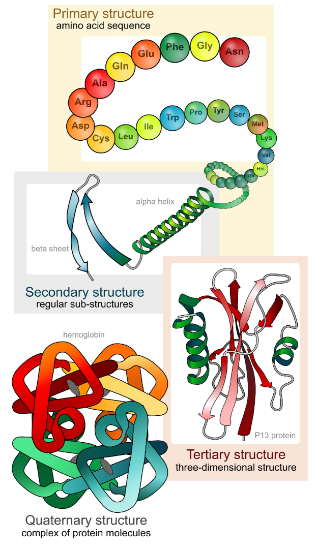
Figure 1.1: Visual of the different levels of description distinguished in the study of proteins, from primary to quaternary structure. In the primary structure, the different amino acids are usually denoted by a three letter code. Image taken from [1].

One of the burning issues in biophysics is the folding and unfolding of proteins. Why? On the one hand, most proteins in the body work properly just in their folded state. Nevertheless, there are misfolded states, metastable in a physical language; proteins in these states are responsible for some diseases as Alzheimer’s, Parkinson’s or the bovine spongiform encephalopathy [2, 3]. This fact can be intuitively understood with the nice parallelism between protein folding and origami figures depicted in figure 1.2. It is when the mechanism responsible for discarding the misfolded proteins—that is, throwing them into the trash—does not properly work that these diseases appear. On the other hand, there are also proteins with mechanical functions that unfold during the extension of muscles. Hence, it is natural that a huge community of biophysicists tries to improve our current understanding of the processes of folding and unfolding [4].

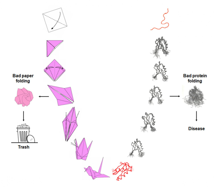
Figure 1.2: Origami analogy of the folding process in proteins. Misfolded states are responsible for different diseases. Image taken from [5].

1.1.1 Single-molecule experiments

The development of the so-called single-molecule experiments in the last decades has triggered a whole new area of investigation on the elastomechanical properties of biomolecules [6, 7, 8, 9]. Up to that breakthrough, experiments were carried out in bulk. In bulk experiments, many particles are involved and thus the only information obtained was about average and collective behavior.

The most used single-molecule techniques are laser optical tweezers (LOT) and atomic force microscopy (AFM). In the LOT case, the molecule is caught between two beads that are optically trapped by lasers. In turn, in the AFM case, the molecule is tightened between a subtract and the tip of a cantilever. AFM excels because of its extensive use and, specifically, has played a crucial role in the study of modular proteins [10, 11, 12]. Figure 1.3 shows a sketch of the experimental setup in a pulling experiment of a molecule comprising two modules. The biomolecule is stretched between the platform and the tip of the cantilever. The spring constant of the cantilever is $k_{c}$, which is usually in the range of $10-100$ pN/nm [13]. The stretching of the molecule makes the cantilever bend by $\Delta X$, and then the force can be recorded as $F=k_{c}\Delta X$. The total length of the whole system $\Delta X+L$, is the sum of the bending of the cantilever and the molecule’s elongation.

Usually, AFM can operate in two modes depending on the control parameter, either length or force. In length control experiments, the position of the platform where the sample rests is controlled by a piezoelectric material and the resulting force is measured. In force control experiments, the force is controlled by a feedback algorithm and the length is recorded. Therefore, in both modes the output of the experiment is a force-extension curve. This force-extension curve provides a fingerprint of the elastomechanical properties of the molecule under study.

Here, we focus on length control experiments with “modular biomolecules”. With this general terminology we allude to both polyproteins [14, 15] (proteins comprising smaller protein modules or domains) and structurally simpler proteins with intermediate states stemming from the unfolding of stable substructures named “unfoldons” [16, 17], see below. The heterogeneity of natural polyproteins makes it quite complicate to study them. For that reason, the generation of artificial engineered homopolyproteins [18, 19], proteins composed of identical (or very similar) repeats, has been a milestone in the advancement of single-molecule experiments.

When a modular biomolecule is pulled in a length control AFM experiment, a sawtooth pattern comes about in the force-extension curve [10, 11, 12], as sketched in figure 1.3. The force generally increases with the length as an indication of the resistance of the biomolecule to stretch under the applied mechanical load. However, at certain values of the length, there are almost vertical “force rips”, marking the unfolding of one of the units: its abrupt unfolding entails a force relaxation, similar to the one found when untying a knot in a rope. Probably, due to its length and relatively stiff nature, one of the most paradigmatic force-extension curve is that of homopolyproteins comprising several immunoglobulin domains of titin, which is the largest known protein in vertebrates [20].

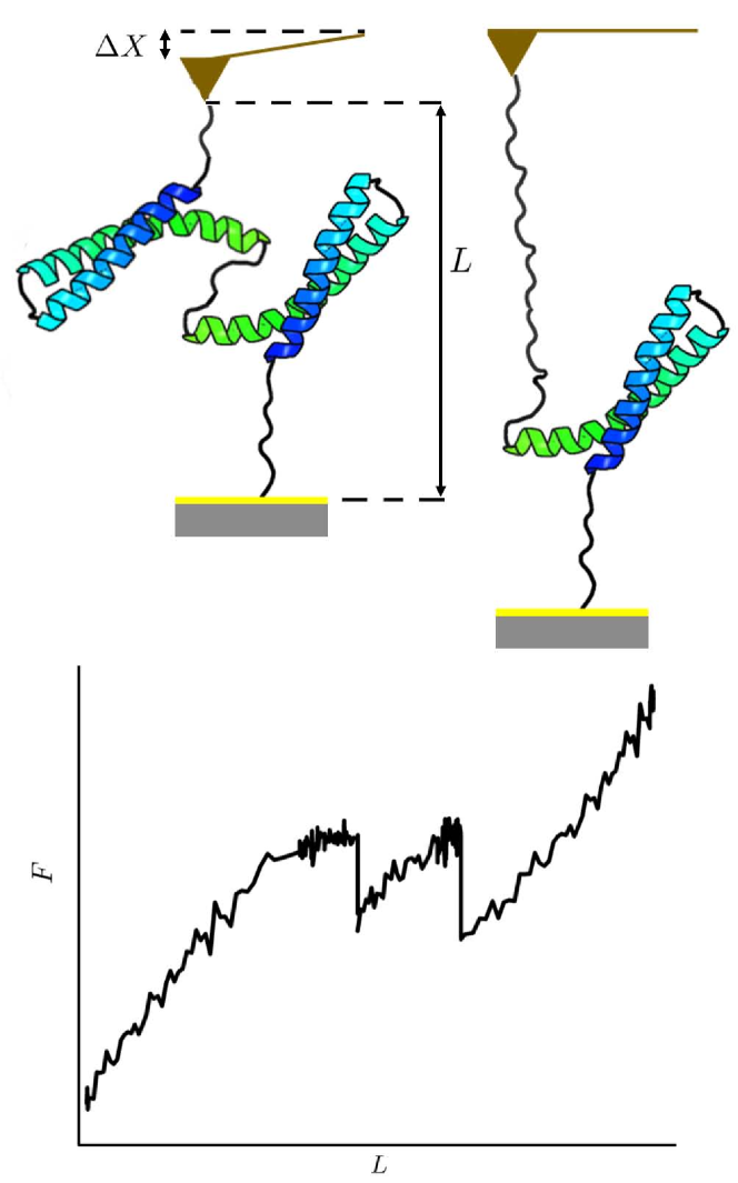
Figure 1.3: (Top) Sketch of the experimental setup in an AFM experiment with a modular biomolecule comprising two modules. On the left, the position of the platform has been shifted, producing an elongation $L$ of the molecule and bending the cantilever a magnitude $\Delta X$. On the right, the force is almost relaxed because of the unraveling of one of the modules. (Bottom) Typical force-extension curve output of the length control AFM experiment above. The rips in the force account for the unfolding of the modules.

1.1.2 Theoretical developments

Biomolecules are particularly appealing systems from a statistical mechanics perspective. Consider that $N$ is the number of atoms that the system comprises. In biomolecules, we have $1\ll N\ll N_{A}$, $N_{A}$ being the Avogadro number. Since relative fluctuations typically scale with $1/\sqrt{N}$, theorists are interested in biomolecules as a perfect laboratory for the development of the thermodynamics of small systems. Herein, we have enough constituent particles to use statistical mechanics arguments, but the fluctuations are still really important [21].

One of the most relevant achievements made by the thermodynamics of the small systems is the derivation of fluctuation theorems. They link equilibrium observables of the system with work functionals in irreversible, nonequilibrium, processes. The first of these theorems is given by Jarzynski equality [22, 23], which was later generalized by Crooks [24, 25]. Starting from work measurements in single-molecule experiments with biomolecules [26], these relations have been used to reconstruct their free energy landscapes.

Polymer physics provides the two most paradigmatic elasticity models of biomolecules: the freely-jointed chain (FJC) and the worm-like chain (WLC) [27, 28]. The main goal of these models is to give an equilibrium force-extension curve for the system. The FJC model considers a concatenation of rigid rods of fixed length with no internal interaction at all, whereas the WLC emerges after considering a continuous chain with elastic energy due to its bending, as sketched in figure 1.4. Let $\bm{r}(s)$ be the parametrization of the curve describing the polymer as a function of its arc length, the unitary tangent vector of the chain is given by

$$\bm{t}=\frac{\partial\bm{r}}{\partial s}.$$ (1.1)

This vector can be decomposed into the perpendicular and parallel to the force directions, with components $\bm{t}_{\perp}$ and $\bm{t}_{\parallel}$, respectively. Specifically, we have that

$$\bm{t}_{\parallel}=(\bm{t}\cdot\bm{u}_{\parallel})\bm{u}_{\parallel},\qquad\bm{u}_{\parallel}=\frac{\bm{F}}{|\bm{F}|},$$ (1.2)

and $\bm{t}_{\perp}=\bm{t}-\bm{t}_{\parallel}$. The curvature $\kappa$ is defined by

$$\kappa\equiv\left|\frac{\partial\bm{t}}{\partial s}\right|=\left|\frac{\partial^{2}\bm{r}}{\partial s^{2}}\right|.$$ (1.3)

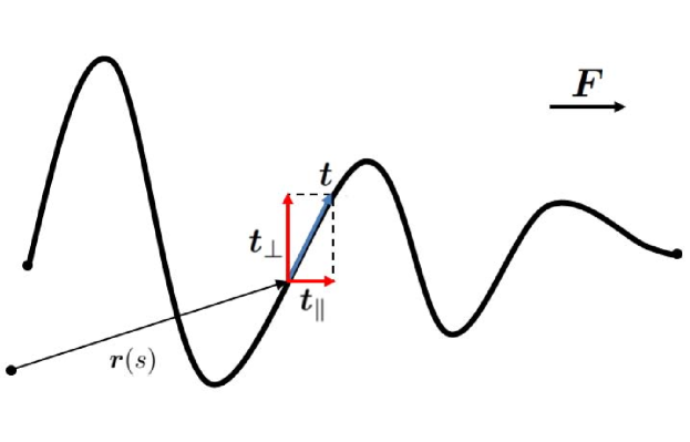
Figure 1.4: Sketch of the WLC model. The protein chain tends to align with the pulling force $\bm{F}$.

The energy of the WLC model is given by

$$H=\frac{1}{2}k_{B}TP\int_{0}^{L_{c}}\!\!\!\!ds\,\kappa^{2}(s)-FL.$$ (1.4)

The first term stands for the energy due to the bending of the polymer. Therein, $k_{B}$ is the Boltzmann constant, $T$ is the temperature, and $P$ is a parameter called the persistence length that gives the characteristic length scale for bending. The longer the persistence length, the larger the bending contribution of the energy. The maximum value of $s$ is the contour length $L_{c}$, which corresponds to the length of the fully extended polymer. The second term on the rhs of (1.4) stands for the energy associated with the pulling force, where

$$L=\int_{0}^{L_{c}}ds\,\bm{t}\cdot\bm{u}_{\parallel}$$ (1.5)

is the projection of the length of the polymer onto the force direction. Of course, $|L|$ is upper bounded by the contour length $L_{c}$, $L=L_{c}$ in the fully extended configuration for which $\bm{t}_{\perp}=\bm{0}$ ($\kappa=0$).

Both the equilibrium force-extension curves of the FJC and WLC models give a harmonic response for small enough stretching, that is $F\propto L$. On the contrary, in the limit of strong pulling the extension of the system approaches its contour length $L_{c}$ and the force diverges as either $(L-L_{c})^{-1}$ for the FJC model, or $(L-L_{c})^{-2}$ for the WLC model. Both the FJC and WLC models have been used for fitting real experiments with biomolecules, giving reasonably good results [29, 30, 31]. Specifically, the following WLC fit [29]

$$\frac{FP}{k_{B}T}=\frac{L}{L_{c}}+\frac{1}{4}\left(\frac{L_{c}}{L_{c}-L}\right)^{2}-\frac{1}{4},$$ (1.6)

is asymptotically valid along all the length range, and it is intensively employed in the literature.

However, the aforementioned paradigmatic models do not take into account the internal structure of the chain. In fact, the internal structure of the biomolecule is responsible for its different states, folded or unfolded for instance. A coarse-grained modeling usually involves considering each unit within a macromolecule as a two-state system, which can be in either a folded or an unfolded state. To account for this, some models [32, 33, 34] consider a WLC with several possible values of the contour lengths: each branch of the force extension curve is fitted by a WLC model with a different value of contour length. Transitions between folded and unfolded states typically follow the development of Kramers theory [35, 36] carried out by Bell [37] and Evans [38]. The Bell-Evans expression provides the transition rates between states, given the applied force and the details of the free energy barrier.

Quite recently, some more theoretical models [39, 40, 41], closer to the approach that will be followed in this thesis, have been proposed to analyze the elasticity of modular biomolecules. These models successfully explain the sawtooth pattern observed in the experiments: interestingly, an equilibrium-statistical-mechanics theory is sufficient to understand their emergence. In a nutshell, the models start from a free energy where each module gives an additive contribution thereto, the individual contributions being double well functions of the corresponding unit’s extension. By maximizing the probability distribution function within the right statistical ensemble (force-control or length-control), or equivalently minimizing the corresponding free energy, the equilibrium force-extension curve of the system is obtained. As a consequence of the different metastable configurations (folded or unfolded) for each module, the force-extension curve presents different branches, see top left panel of figure 1.5.

When dynamics is incorporated, hysteresis processes might appear. In figure 1.5, some force-extension curves of a system of 8 units for different velocities are shown. The hysteretic behavior strongly depends on the pulling rate employed. More specifically, an interesting interplay between the pulling velocity and the temperature is observed. At a certain value of the temperature, the system mainly sweeps the equilibrium force-extension curve if the pulling speed is slow enough: this is the quasistatic regime of pulling (bottom left). However, for higher velocities, hysteresis comes about (top right). This phenomenon is accentuated as the temperature is lowered, since thermally activated transitions are not possible in “cold” systems. This allows the system to sweep the whole metastable branches (bottom right), a regime that is usually said to correspond to the “maximum hysteresis path” [42] (also adiabatic pulling [41]).

In fact, the maximum hysteresis path regime described above stems from the interplay between the pulling velocity and the temperature: the pulling velocity must be slow enough to allow the system to move over the (metastable) equilibrium branches but fast enough to prevent the system from going from the folded to the unfolded basin (or vice versa) by thermal activation. This regime will be of crucial relevance in the development of the theory presented in part I of this thesis.

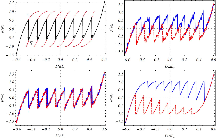
Figure 1.5: (Top left) Equilibrium force rips in the force-extension curve for a system with 8 units (length-control). Different colors are used to represent the stability: solid black for stable parts, dotted red for metastable parts and black arrows for force rips. In a quasistatic pulling process, the system follows the solid black curve with a series of first-order transitions in the force. (Top right) Hysteresis cycle for a system composed of 8 units, at a relatively high pulling speed and moderate temperature. Two traces are plotted: solid blue for unfolding and dashed red for refolding. (Bottom left) Same plot as in the top right panel, but for a smaller pulling velocity. Aside from thermal fluctuations, the system almost sweeps the equilibrium curve: the pulling is basically quasistatic (Bottom right) The same plot as in the bottom left panel, but for an almost vanishing temperature. Thermal fluctuations are so small that the system approaches the $T=0$ behavior (adiabatic pulling): therein, the branches are swept up to the end of the metastability region. Taken from [41].

1.1.3 Unfolding pathway and its pulling dependence

The unfolding pathway is, roughly, the order and the way in which the structural blocks of a macromolecule unfold. The force-extension curve obtained in single-molecule experiment characterizes the elastomechanical behavior of the macromolecule and provides basic and essential information about the unfolding pathway. Some studies show that the pulling velocity plays a relevant role in determining the unfolding pathway, see for example [12, 43, 17, 44].

Different unfolding pathways have been observed depending on (i) pulling direction, that is, which of the ends (C-terminus or N-terminus) the molecule is pulled from and (ii) the pulling speed [12, 43, 17, 44]. Intuitively, it has been claimed that it is the inhomogeneity in the distribution of the force across the protein, for high enough pulling speeds, that causes the unfolding pathway to change [17]. Nevertheless, to the best of our knowledge, a theory that explains this crossover is still lacking.

Our interest in this problem was triggered by the dissenting unfolding pathway observed in the maltose binding protein (MBP) in experiments [16] and simulations for high pulling velocity [17]. This molecule unfolds in four steps, which led Bertz and Rief to identify four internal substructures they call “unfoldons”, see figure 1.6. More specifically, AFM experiments allowed them to characterize these four unfoldons in the MBP, labeling them as M1, M2, M3 and M4, with M1 being the closest to the C-terminus and M3 the closest to the N-terminus [16]. Pulling the molecule at a typical speed of $10^{-9}$ nm/ps, Bertz and Rief found a well-defined unfolding pathway: the weakest unfoldon (M1), that is, the one characterized by the lowest opening force, unraveled first. Thereafter, the remainder of the unfoldons opened sequentially, from weakest to strongest (M4).

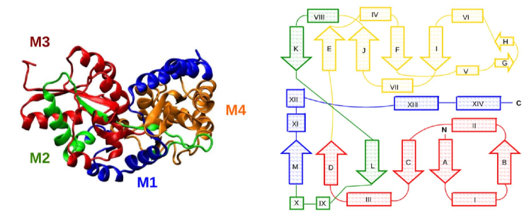
Figure 1.6: Structure of the Maltose Binding Protein (PDB ID: 4MBP). The color code identifies the four unfoldons: M1 blue; M2 green; M3 red; M4 gold. (Left) Crystallographic structure. (Right) Topological diagram. Taken from [17].

Later, Guardiani et al. had a more detailed look into the unfolding of the MBP [17]. They showed, by means of a combination of G$\overline{\mbox{o}}$ model simulations and steered molecular dynamics, that the unfolding pathway is more complex and seems to depend on both the velocity and direction of pulling. C-pulling simulations of the G$\overline{\mbox{o}}$ model always showed a pathway compatible with Bertz and Rief’s experiment, see top panel of figure 1.7. However, N-pulling simulations of the G$\overline{\mbox{o}}$ model displayed a different behavior: for small velocities, again Bertz and Rief’s pathway was found, but for high enough pulling speed it was M3, the closest to the N-terminus, that opened first, as shown in the bottom panel of figure 1.7. Steered molecular dynamics simulations at a pulling speed of $5\cdot 10^{-3}$ nm/ps gave results that were consistent with those from the G$\overline{\mbox{o}}$ model at high velocities, showing the different pathways (M1 vs. M3 opening first) depending on the pulled terminus (C vs. N).

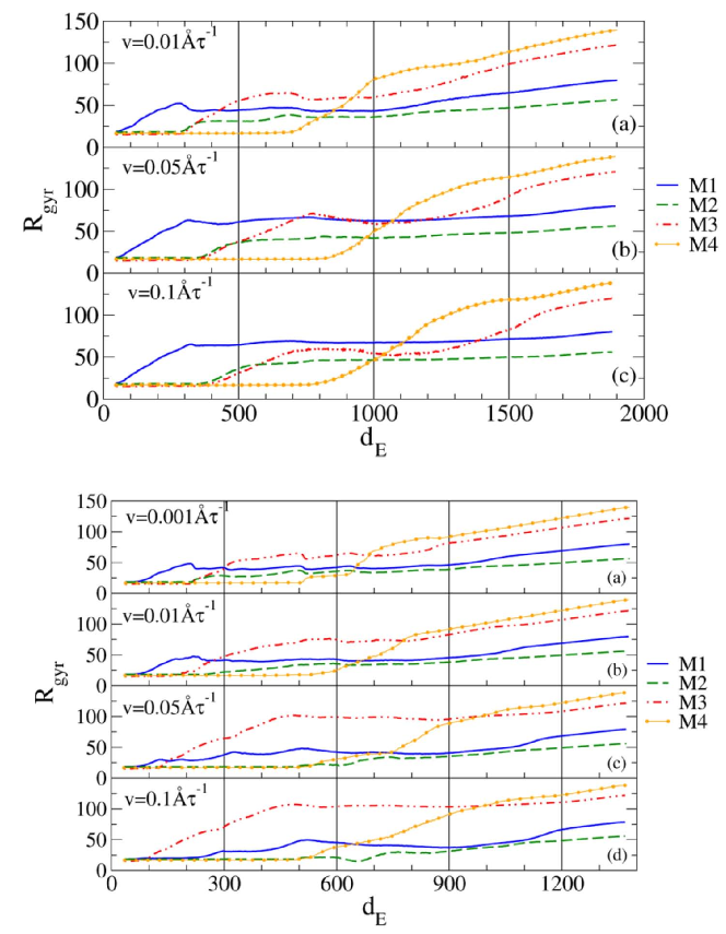
Figure 1.7: Evolution of the gyration radius for unfoldons M1, M2, M3, and M4 as functions of the end-to-end distance (Å) at different pulling speeds. The curves show averages over 50 runs of simulations of the G$\overline{\mbox{o}}$ model, for C-pulling (above) and N-pulling (bottom). For C-pulling, it is always M1, the weakest unfoldon, that opens first (solid blue line). Notwithstanding, for N-pulling, the first unfoldon that unravels depends on the pulling velocity: for slow pulling ($v=0.001\text{\AA}\tau^{-1}$) it is still M1, but for fast enough pulling ($v=0.1\text{\AA}\tau^{-1}$) it is M3, the closest to the pulled end as depicted in figure 1.6 (dot-dashed red line). Taken from [17].

In this context, Guardiani et al. introduced in [17] a toy model to qualitatively explain the observed pathways, which is the starting point of part I of this thesis. This simple model is akin to those employed in [39, 40, 41] to investigate the force-extension curves of modular proteins, their main difference stemming by the incorporation—in the simplest way—of the spatial structure of the chain into Guardiani et al.’s model. Numerical simulations of the latter presented a phenomenology that was compatible with both the G$\overline{\mbox{o}}$ model and the steered molecular dynamics results [17]. One of our aims is to develop a theoretical framework for this simple model, in order to get a deeper understanding of the dependence of the unfolding pathway on the pulling velocity and direction.

1.1.4 Summary of part I

Despite the large number of models developed to unravel the nature of biomolecules, not everything is neat. In part I, we attempt both to better understand and to predict the unfolding pathway of modular biomolecules.

Our approach to this problem follows the philosophy presented above, we put forward a simple model with the minimal ingredients to grasp the essence of the system. We do so in chapter 2. Therein, we introduce the model, which portrays the conformation of the protein into a 1d chain with different units. Each unit contributes to the global free energy with a function that only depends on its own extension with a double-well shape. The perturbative solution of the dynamical system leads to our predicting of the first module that unfolds. Numerical results are in excellent agreement with our theoretical predictions. Additionally, we carry out some modifications of the model, in order to get closer to real experiments. The results are unchanged at the lowest (leading) order, thus proving the robustness of our analysis.

Finally, we test the theoretical scheme developed in chapter 2 in a simple biomolecule, which comprises two coiled-coil structures, in chapter 3. This analysis is carried out by means of steered molecular dynamics simulations of the coiled-coil construct. First, characterizing the molecule is required: in particular, we need to introduce a criterion for considering it unfolded or folded. Such a criterion allows us to make a systematic comparison with the theoretical framework. A thorough statistical study of the simulations output provides a significant test of theory and validates the usefulness of the approach.

Some technical details that are omitted in the main body of this part of the thesis are given in appendix A.

1.2 Granular gases

A granular material is made of macroscopic particles that are called grains [45, 46]. They can be found almost everywhere, for example dust, sand, seeds, pills, iceberg groups or asteroid populations are all instances of granular matter. Improving our knowledge of granular matter has a clear technical, industrial, and even economic interest. To support this statement, it suffices to turn our thoughts to transport and storage industry, agriculture or construction. In figure 1.8, some typical examples of granular material are shown.

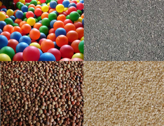
Figure 1.8: Some examples of granular matter: balls, gravel, lentils and sesame seeds. Taken from [47].

All granular materials share some typical properties. First, grains are solid and macroscopic, that is, their dynamics is governed by classical mechanics laws and they fill a space that is excluded to the other grains. Second, their interactions are nonconservative in the following sense: when two grains collide, some of their energy is “lost” into internal degrees of freedom, mainly due to deformation, as heat. Third, the characteristic energy of a grain is much greater than the thermal energy. Therefore, the temperature of the medium in which the grains are immersed is largely irrelevant: the typical energy to lift a grain by its own diameter is several orders of magnitude larger than the thermal energy [48]. Indeed, in granular fluids one can define a relevant granular temperature from kinetic theory, linked to velocity fluctuations. This granular temperature has nothing to do with the “conventional” temperature, which as already stated plays no role, but is related to the energy injection mechanism that is needed to keep grains moving.

The result of enclosing a granular material and shaking it rapidly is a fluidized granular material: the granular fluid that we have just referred to above. The amount of available space and the intensity of the shaking determine the regime of fluidization [49]. When interactions are dominated by two-particle instantaneous (hard-core-like) collisions, one usually speaks of a granular gas. This regime is typically achieved in experiments when the packing fraction is of the order of $\sim\!1\%$ or less, and the peak acceleration is many times the gravity acceleration.

The gas regime has played a crucial role in the development of granular kinetic theory: in the dilute limit, one may retrace the classical molecular kinetic theory after having relaxed the constraint of energy conservation [50]. Granular collisions are, in fact, inelastic: this occurs because each grain is approximated as a rigid body and the collisional internal dynamics is replaced by an effective energy loss, usually characterized by a normal restitution coefficient $\alpha\in(0,1]$. This is the smooth hard-particle model: particles only interact when at contact, then the component of the relative velocity along the direction joining their centers is reversed and shrunk by a factor $\alpha$, whereas the other components remain unchanged. Therefore, $\alpha=1$ corresponds to elastic collisions, whereas $\alpha\to 0$ describes the completely inelastic limit.

Most of granular kinetic theory rests upon many variants of the basic model of smooth hard particles. Important variants include roughness and rotation [51, 52, 53, 54, 55] as well as the consideration of velocity-dependent inelasticity [56]. Notwithstanding, the simple model of smooth inelastic hard spheres suffices to explain the basic phenomenology of granular gases. In this context, the Boltzmann equation for inelastic hard spheres constitutes the foundation of many investigations in the realm of granular phenomena, with both numerical and analytical approaches [57].

Granular fluids exhibiting separation between fast microscopic scales and slow macroscopic ones have led to several procedures to build a granular hydrodynamics [58, 59]. Note that the scale separation hypothesis is less clear in the granular case, as compared to molecular gases. First, one has the spontaneous tendency of granular gases to develop strong inhomogeneities even at the scale of a few mean free paths. Second, a granular system is typically of “small” size: it is usually constituted by a few thousands of grains [60, 61]. The latter limitation cannot be easily relaxed even in theoretical studies: stability analyses have shown that spatially homogeneous states are unstable for too large sizes in some typical states [62].

The intrinsic “small” size of granular gases makes it essential to address another task: an adequate and consistent description of fluctuations, which are always important in a small system [63, 64, 65]. The number of particles $N$, ranging from $10^{2}$ to $10^{4}$, is large enough to make it possible to apply the methods of statistical mechanics, but definitely much smaller than the Avogadro number. Interestingly, this is also the case for biomolecules, as stated before in section 1.1.2; the special relevance of fluctuations is a point that links the two parts of this thesis.

Unfortunately, there is no general theory currently available for mesoscopic fluctuations out-of-equilibrium. Notwithstanding, important steps in the deduction of a consistent fluctuating hydrodynamics for inelastic hard spheres have been recently taken in the context of kinetic theory [66]. In this regard, the quite broad framework of Macroscopic Fluctuation Theory [67] cannot be employed. In its current state of development, Macroscopic Fluctuation Theory does not include macroscopic equations with advection terms and momentum conservation, such as those in the “granular” Navier-Stokes equations.

In the last decades, lattice models have proved to be a flexible tool to identify the essential steps in a rigorous approach to the hydrodynamic limit, both at the average [68, 69] and fluctuating [67] levels of description. Fluctuating hydrodynamics in linear and nonlinear lattice diffusive models have been recently investigated, both in the conservative [70, 71, 72, 73] and in the nonconservative cases for the energy field [74, 75, 76, 77, 78]. Later, a lattice model, which in some simplified way mimics the velocity field of a granular gas, has been put forward to incorporate momentum conservation [79]. This model is the central pillar of our investigations in part II of this thesis.

1.2.1 Granular hydrodynamics

Evolution equations for the “slow” fields, in space $\bm{r}$ and time $t$, density $n(\bm{r},t)$, velocity $\bm{u}(\bm{r},t)$, and granular temperature $T(\bm{r},t)$ constitute the full granular hydrodynamics. These equations can be derived from the Boltzmann equation for inelastic hard spheres, through a Chapman-Enskog procedure closed at the Navier-Stokes order [59, 46]. For generic dimension $d$, they are given by

$$\partial_{t}{n}+\nabla\cdot(n\bm{u}) =0,$$ (1.7a)

$$\partial_{t}{\bm{u}}+\bm{u}\cdot\nabla\bm{u}+(nmk_{B})^{-1}\nabla\cdot\mathcal{P} =0,$$ (1.7b)

$$\partial_{t}{T}+\bm{u}\cdot\nabla T+\frac{2}{dnk_{B}}\left[\mathcal{P}:(\nabla\bm{u})+\nabla\cdot\bm{q}\right]+\zeta T =0,$$ (1.7c)

in which $m$ is the mass of the particles. The energy dissipation rate is $\zeta(\bm{r},t)>0$, being $\zeta\to 0$ in the elastic limit, while the pressure tensor $\mathcal{P}(\bm{r},t)$ and the heat flow $\bm{q}(\bm{r},t)$ read

$$\mathcal{P}_{ij}=p\delta_{ij}-\eta\left(\nabla_{i}u_{j}+\nabla_{j}u_{i}-\frac{2}{d}\delta_{ij}\nabla\cdot\bm{u}\right),\quad\bm{q}=-\kappa\nabla T-\mu\nabla n.$$ (1.8)

Additionally, the bulk pressure $p$, the shear viscosity $\eta$, the heat-temperature conductivity $\kappa$ and the heat-density conductivity $\mu$ are given by constitutive relations [46]. We briefly recall that the transport coefficients depend on the hydrodynamic fields. Specifically, for hard-spheres one has that $\eta\sim\sqrt{T}$, $\kappa\sim\sqrt{T}$, $\mu\sim n^{-1}T^{3/2}$ and $\zeta\sim n\sqrt{T}$ [46].

This thesis is not an exhaustive investigation of granular hydrodynamics and its rich catalog of possible stationary and nonstationary regimes [50, 49]. Our aim is to study the model introduced in part II, validating its use for the simplified investigation of some peculiar states in the granular realm. With this intention, we highlight three essential aspects that give some contact points of the aforementioned model with actual granular fluids. First, the existence of a spatially homogeneous nonstationary solution, that is, the “Homogeneous Cooling State” (HCS). Second, the instability of such a state with respect to perturbations with long enough wavelength (small enough wavenumber). And third, the existence of the Uniform Shear Flow (USF) stationary state, in which the energy loss due to collisions is balanced—on average—by the heating brought about by the velocity difference, that is, the shear, imposed between the system boundaries [80]. All such aspects stem from a key difference with respect to the hydrodynamics of molecular fluids, which is the presence of the energy sink term $\zeta T$ in (1.7).

When spatial homogeneity is assumed along with periodic boundary conditions, and initial conditions $n(\bm{r},t=0)=n$, $u(\bm{r},t=0)=0$, and $T(\bm{r},t=0)=T(0)$, (1.7) are reduced to

$$\dot{T}(t)=-\zeta(t)T(t).$$ (1.9)

Since $\zeta(t)\propto T(t)^{1/2}$ for hard-spheres, (1.9) leads to the well known Haff’s law [81]

$$T_{\text{\tiny HCS}}(t)=T(0)\left[1+\frac{\zeta(0)t}{2}\right]^{-2}.$$ (1.10)

A different collisional model that is often used to simplify the kinetic theory approach is the so-called gas of pseudo-Maxwell molecules [82]: its peculiarity is that $\zeta(t)=\zeta(0)$ is constant and therefore Haff’s law simplifies to an exponential decay,

$$T_{\text{\tiny HCS}}(t)=T(0)\exp[-\zeta(0)t].$$ (1.11)

This spatially homogeneous solution, with monotonically decreasing temperature, is generally called “Homogeneous Cooling State” (HCS). Of course, it can be predicted at the more fundamental and general level of the Boltzmann [83] or even Liouville[84] equations.

The HCS is not stable if the system size exceeds some critical value. Spatial perturbations of the velocity and density fields are amplified when the system is large enough [85, 62]. A linear stability analysis shows that the fastest amplification usually occurs for shear modes, which correspond to a transverse perturbation of the velocity field. For instance, a nonzero $y$ component of $\bm{u}$ modulated along the $x$ direction, that is, $u_{y}(x,t)$. The critical wavelength $L_{c}$ separating the stable from the unstable regime depends upon the restitution coefficient as

$$L_{c}^{2}\propto(1-\alpha^{2})^{-1}.$$ (1.12)

Velocity perturbations are not really amplified, because the amplitude of their fluctuations (temperature) always decay: the instability is observed only when the rescaled velocity field $u(\bm{r},t)/\sqrt{T_{\text{\tiny HCS}}(t)}$ is considered. Perturbations in the other fields (density, longitudinal velocity and temperature), the evolution of which are coupled with the velocity field, are also amplified, but with a slower rate and for longer wavelengths.

There is a range of system sizes such that the only linearly unstable mode is the shear mode [50]. This entails that the velocity field is incompressible and density does not evolve from its initial uniform configuration. Such a regime may be observed for a certain amount of time, longer and longer as the elastic limit is approached. In two dimensions, (1.7) is obeyed with constant density and, for instance, $u_{x}=0$ whereas the hydrodynamic fields $u_{y}$ and $T$ only depend on $x$. In this situation, we have that (1.7) reduces to

$$\partial_{t}{u_{y}(x,t)} =(nm)^{-1}\partial_{x}[\eta\partial_{x}u_{y}(x,t)],$$ (1.13a)

$$\partial_{t}{T}(x,t) =\frac{1}{nk_{B}}\eta[\partial_{x}u_{y}(x,t)]^{2}+\frac{1}{n}\partial_{x}[\kappa\partial_{x}T(x,t)]-\zeta T.$$ (1.13b)

In section 4.1.3 we will see that our lattice model is well described, in the continuum limit, by completely analogous equations.

It is interesting to put in evidence a particular stationary solution of the system (1.13). Seeking time-independent solutions thereof, one finds

$$\partial_{x}[\eta\partial_{x}u_{y}^{(\text{s})}(x)]=0,\quad\frac{\eta}{k_{B}}[\partial_{x}u_{y}^{(\text{s})}(x)]^{2}=-\partial_{x}[\kappa\partial_{x}T^{(\text{s})}(x)]+n\zeta T^{(\text{s})}(x).$$ (1.14)

The general situation is that both the average velocity and temperature profiles are inhomogeneous: this is the so-called Couette flow state, which also exists in molecular fluids. Nevertheless, in granular fluids, there appears a new steady state in which the temperature is homogeneous throughout the system, $T^{(\text{s})}(x)=T$, and the average velocity has a constant gradient, $\partial_{x}u=a$: this is the Uniform Shear Flow (USF) state, characterized by the equations

$$\partial_{x}^{2}u_{y}^{(\text{s})}(x)=0,\quad\eta[\partial_{x}u_{y}^{(\text{s})}(x)]^{2}=nk_{B}\zeta T^{(\text{s})}.$$ (1.15)

Such a steady state is peculiar of granular gases where the viscous heating term is locally compensated by the energy sink term. In granular gases of hard spheres, it has been proven that the USF state is linearly stable for perturbations in the direction of the shear [86].

1.2.2 Irreversibility: $H$-theorem

In thermodynamics and statistical mechanics, proving the global stability of the equilibrium state—or, in general, of the relevant stationary state—usually involves the introduction of a suitable Lyapunov functional [87]. A Lyapunov functional of the probability distribution function (PDF) has the following three properties:

• It is bounded from below.

• It monotonically decreases with time.

• Its time derivative vanishes only when the PDF is the equilibrium one.

Therefore, in the long time limit, the Lyapunov functional must tend to a finite value and thus its time derivative vanishes. As a consequence, any PDF, corresponding to an arbitrary initial preparation, tends to the equilibrium PDF. This rigorously proves that the equilibrium state is irreversibly approached and said to be globally stable.

One of the most relevant examples of such a Lyapunov functional is the renowned Boltzmann $H$-functional. At the Boltzmann level of description, the nonequilibrium behavior of a dilute gas is completely encoded in the one-particle velocity distribution function $f(\bm{r},\bm{v},t)$. After introducing the Stosszahlansatz or molecular chaos hypothesis, Boltzmann derived a closed nonlinear integro-differential equation for $f(\bm{r},\bm{v},t)$ governing its time evolution [88]. Also, for spatially homogeneous states, he showed that the functional $H_{B}[f]=\int d\bm{v}f(\bm{v},t)\ln\!f(\bm{v},t)$ has the three properties of a Lyapunov functional. This $H$-theorem shows that all solutions of the Boltzmann equation tend in the long time limit to the Maxwell velocity distribution.

Thus, irreversibility naturally stems from a reversible molecular picture [89, 90]. Indeed, a key point for deriving the $H$-theorem is the reversibility of the underlying microscopic dynamics. This almost paradoxical interplay between reversibility and irreversibility has not been entirely absent of controversy [91, 92, 93]. In an inhomogeneous situation, one has to consider the spatial dependence of the one-particle distribution function $f(\bm{r},\bm{v},t)$, and the above functional must be generalized to

$$H_{B}[f]=\int d\bm{r}\,d\bm{v}f(\bm{r},\bm{v},t)\ln\!f(\bm{r},\bm{v},t).$$ (1.16)

With an additional assumption about the smoothness of the walls of the gas container, in order to avoid energy transport through them, it can also be shown that (1.16) is a nonincreasing Lyapunov functional in the conservative case [94].

In the realm of Markovian stochastic processes, we find another example of Lyapunov functionals. Therein, the stochastic process $X(t)$ is completely determined by its conditional probability density $P_{1|1}(X,t|X_{0},t_{0})$ of finding the system in state $X$ at time $t$, given it was in state $X_{0}$ at time $t_{0}$, and the probability density $P(X,t)$ of finding the system in state $X$ at time $t$ [95]. Both probability densities satisfy a master equation, but with different initial conditions: the first verifies $P_{1|1}(X,t_{0}|X_{0},t_{0})=\delta(X-X_{0})$, whereas for the latter $P(X,t_{0})=P_{\text{ini}}(X)$, with $P_{\text{ini}}(X)$ corresponding to the arbitrary initial preparation.

When the Markovian stochastic process under scrutiny is irreducible or ergodic, that is, every state can be reached from any other state by a chain of transitions with nonzero probability, there is only one stationary solution of the master equation. In physical systems, this steady solution must correspond to the equilibrium-statistical-mechanics distribution $P_{\text{eq}}(X)$. Moreover, a Lyapunov functional can be constructed,

$$\mathcal{H}[P]=\int dXP_{\text{eq}}(X)\,g\!\left[\frac{P(X,t)}{P_{\text{eq}}(X)}\right],$$ (1.17)

where $g(x)$ is any positive-definite convex function ($g^{\prime\prime}(x)\geq 0$). It must be stressed that the proof of this $H$-theorem for master equations rely only on the ergodicity of the underlying microscopic dynamics. It is not necessary to assume detailed balance, which is connected with the reversibility of the underlying microscopic dynamics [95].

The most usual choice for $g$ is $g(x)=x\ln x-x+1$, which leads to the Kullback-Leibler divergence [96]

$$\mathcal{H}[P]=\int dXP(X,t)\,\ln\!\left[\frac{P(X,t)}{P_{\text{eq}}(X)}\right].$$ (1.18)

This choice has the physical advantage of $\mathcal{H}[P]$ being “extensive”: if the system at hand comprises two independent subsystems $A$ and $B$, so that $dX\equiv dX_{A}dX_{B}$ and $P(X)=P_{A}(X_{A})P_{B}(X_{B})$, one has that $\mathcal{H}[P]=\mathcal{H}_{A}[P_{A}]+\mathcal{H}_{B}[P_{B}]$. This feature is desirable since usually one considers $-\mathcal{H}$ to define a nonequilibrium entropy $S$. In this way, the nonincreasing behavior of $\mathcal{H}$ leads to a nondecreasing time evolution of $S$. Moreover, in this way $\mathcal{H}[P]$ remains invariant upon a change of variables $Y=f(X)$ [97, 98].

Although the Boltzmann equation is not a master equation, we may wonder why the expressions for $H_{B}$ in (1.16) and $\mathcal{H}[P]$ in (1.18) are different. Specifically, we may wonder why not writing

$$H[f]=\int d\bm{r}\,d\bm{v}f(\bm{r},\bm{v},t)\ln\!\left[\frac{f(\bm{r},\bm{v},t)}{f_{\text{eq}}(\bm{v})}\right]$$ (1.19)

for the Boltzmann equation, instead of $H_{B}[f]$. Up to now, we have been implicitly considering the “classic” problem with elastic collisions between particles, in which the system eventually reaches thermodynamic equilibrium. Therein, the answer is trivial: since $\ln f_{\text{eq}}(\bm{v})$ is a sum of constants of motion, $H[f]-H_{B}[f]$ is constant and both are utterly equivalent.

The problem about the existence of an extensive $H$-functional is quite relevant in nonequilibrium statistical mechanics. If there is one, it makes it possible to define a monotonically increasing nonequilibrium entropy $-H$ that extends the Clausius inequality to nonequilibrium states, as already stated above. In this context, it is important to stress that the final state is, in general, not an equilibrium one but a nonequilibrium steady state. Thus, stationarity holds but nonvanishing currents are allowed in the system. In addition, the equilibrium distribution $f_{\text{eq}}$ in $H$ has to be substituted with the stationary one $f_{\text{s}}$. Due to its intrinsically nonequilibrium nature, granular fluids is a benchmark for these investigations.

In granular fluids, functionals $H[f]$ and $H_{B}[f]$ are no longer equivalent: with the stationary PDF, $\ln f_{\text{s}}$ is no longer a sum of constants of motion. Indeed, for granular gases described by the inelastic Boltzmann equation [46, 100], there are some results that hint at $H_{B}$ not being a “good” Lyapunov functional. Within the first Sonine approximation, it has been proven that the time derivative of $H_{B}$ does not have a definite sign in the linear approximation around the steady state [101].

Moreover, Marconi et al. have numerically shown that $H_{B}$ is nonmonotonic and even steadily increases from certain initial conditions [97]. They have also put forward some numerical evidence, further reinforced by García de Soria et al.’s work [98], in favor of $H$ being a “good” Lyapunov functional. Numerical results for the specific case of a uniformly heated inelastic Maxwell model, taken from [97], are reproduced in figure 1.9. In addition, it should be stressed that $H$ is found to be a nonincreasing function in [98] by a combination of three different simulation methods: spectral method, direct simulation Monte Carlo [102, 103], and molecular dynamics.

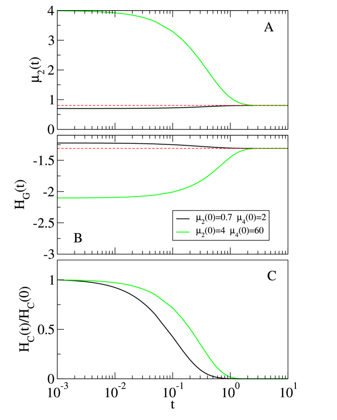
Figure 1.9: Time evolution of different candidates for a Lyapunov functional in a uniformly heated inelastic Maxwell model. Boltzmann’s $H_{B}$ ($H_{G}$ in the notation of Ref. [97]) is shown in panel B , $H$ ($H_{C}$) is shown in panel C, whereas the evolution of the granular temperature to its steady value is displayed in panel A. These numerical results show that $H_{B}$ does not decrease for some situations, in contrast a monotonic decrease of $H$ is always observed. Taken from [97].

These numerical evidences in favor of $H$ being a “good” Lyapunov functional [97, 98] call for further theoretical work. Some attempts at proving such a result have been carried out by García de Soria et al. [98]. Specifically, they have shown that an $H$-theorem holds at the level of the $N$-particle PDF (Kac-like description), with an $H$-functional similar to that in (1.18). Undoubtedly, this proof at the $N$-particle level is a neat step forward in the right direction. However, to the best of our knowledge, there is no rigorous mathematical proof for the $H$-theorem at the level of the one-particle description. In addition, only spatially homogeneous situations, in which the $\bm{r}$-dependence of $f$ and thus the integration over $\bm{r}$ may be dropped, have been analyzed [97, 98].

Wrapping things up, an analytical proof of either global stability or the $H$-theorem is currently unavailable at the level of the kinetic one-particle description for granular gases. This is true even for simple collision terms, such as those corresponding to hard-spheres or the cruder Maxwell molecules model, which are considered in [97, 98]. Therefore, it seems worth investigating this subject in simplified models, like the one introduced in part II of this thesis, for which analytical calculations are expected to be more feasible.

1.2.3 Memory effects: Kovacs experiment

The equilibrium state of physical systems is characterized by the value of a few macroscopic variables, for instance pressure, volume and temperature in molecular fluids. These macroscopic variables provide a full characterization of the system: different samples sharing the same values respond identically to an external perturbation. On the contrary, a system in a nonequilibrium state, even if it is stationary, is not fully characterized by the value of the macroscopic variables: the response to an external perturbation may depend also on additional variables or, equivalently, on its entire thermal history. This behavior unavoidably leads to the emergence of memory effects.

Kovacs carried out a pioneering work in the field of memory effects in nonequilibrium systems [104]. The Kovacs experiment showed that pressure, volume and temperature did not fully characterize the state of a sample of polyvinyl acetate that had been aged for a long time at a certain temperature $T_{1}$. The pressure was fixed during the whole experiment, and the time evolution of the volume was recorded. After a waiting time $t_{w}$, the temperature was suddenly changed to $T$, for which the equilibrium value of the volume equaled its instantaneous value at precisely $t_{w}$. Counterintuitively—from an equilibrium perspective—the volume did not remain constant. Instead, it displayed a hump, passing through a maximum before tending back to its initial equilibrium value.

This effect has extensively been studied in glassy systems [105, 106, 107, 108, 109, 110, 111]. Therein, the relevant physical variable is the energy instead of the volume. First, the system is equilibrated at a “high” temperature $T_{0}$. Then, at $t=0$, the temperature is suddenly quenched to a lower temperature $T$, after which the relaxation function $\phi(t)$ of the energy $E$ is recorded. Specifically, $\phi(t)=\langle E(t)\rangle-\langle E\rangle_{\text{eq}}$, where $\langle E\rangle_{\text{eq}}$ is the average equilibrium energy at temperature $T$. Alternatively, a similar procedure is followed, equilibrating the system again at $T_{0}$, but at $t=0$, the temperature is changed to an even lower value $T_{1}$, $T_{1}<T<T_{0}$. The system relaxes isothermally at $T_{1}$ for a certain waiting time $t_{w}$, such that $\langle E\rangle(t=t_{w})$ equals $\langle E\rangle_{\text{eq}}$. At this time $t_{w}$, the temperature is increased to its corresponding equilibrium value $T$. However, the energy does not remain constant, but displays a hump behavior represented by a function $K(t)$. At first, $K(t)$ increases from zero until a maximum is attained for $t=t_{k}$, and only afterwards, it goes back to zero. Similarly to the relaxation function, we have defined $K(t)=\langle E(t)\rangle-\langle E\rangle_{\text{eq}}$, for $t\geq t_{w}$. Note that $K(t)\leq\phi(t)$ for all times, with the equality being only asymptotically approached in the long time limit. A qualitative plot of the Kovacs effect is depicted in figure 1.10.

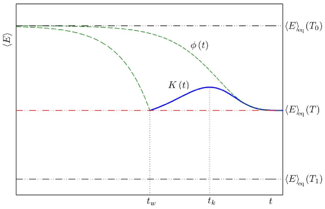
Figure 1.10: Scheme of the Kovacs experiment. The dashed curve on the right, labeled by $\phi(t)$, represents the direct relaxation from $T_{0}$ to $T$. The dashed curve on the left stands for the part of the relaxation from $T_{0}$ to $T_{1}$ that is interrupted at $t=t_{w}$ by the second temperature jump, changing abruptly the temperature from $T_{1}$ to $T$. After this second jump, the system follows the nonmonotonic response $K(t)$, given by the solid line, which reaches a maximum at $t=t_{k}$ and, afterwards, approaches $\phi(t)$ for very long times.

For molecular (thermal) systems, the equilibrium distribution is the canonical one, and it has been shown that, in linear response theory [109],

$$K(t)=\frac{T_{0}-T_{1}}{T_{0}-T}\phi(t)-\frac{T-T_{1}}{T_{0}-T}\phi(t-t_{w}),$$ (1.20)

where the final temperature $T$ and the waiting time $t_{w}$ are related by

$$\frac{T-T_{1}}{T_{0}-T_{1}}=\frac{\phi(t_{w})}{\phi(0)}.$$ (1.21)

In linear response, the relaxation function $\phi(t)$ decays monotonically in time because it is proportional to the equilibrium time correlation function, as predicted by the fluctuation-dissipation theorem. Therefrom,

$$\phi(t)\propto\langle E(0)E(t)\rangle_{\text{eq}}-\langle E\rangle_{\text{eq}}^{2}=\sum_{i}c_{i}\exp(\lambda_{i}t),$$ (1.22)

with $c_{i}>0$ and $\lambda_{i}<0$ for all $i$ [95].

The linear response results above make it possible to understand the phenomenology observed in the Kovacs experiments [109]: (i) the inequality $0\leq K(t)\leq\phi(t)$, which assures that the hump always has a positive sign (from now on, “normal” behavior), (ii) the existence of only one maximum in the hump and (iii) the increase of the maximum height and the shift of its position to smaller times as $t_{w}$ is decreased. Nevertheless, it must be noted that the experiments, both real [104] and numerical [105, 106, 107, 108, 109, 110], are mostly done out of the linear response regime. Therefore, it seems that the validity of these results extends beyond expectations. In fact, it has been checked that the linear approximation still gives a fair description of the hump for not-so-small temperature jumps in simple models [111].

More recently, the Kovacs memory effect has been investigated in granular gases. The simplest case is that of granular gases considered in [112, 113], uniformly heated by the stochastic thermostat introduced in [114, 115, 116, 57]. The value of the kinetic energy, or granular temperature, at the nonequilibrium steady state (NESS) $T_{s}$ is controlled by the driving intensity $\xi$ of the thermostat, $T_{s}=T_{s}(\xi)$. Therefore, a Kovacs-like protocol can be implemented in a completely analogous way to the one described above, with the the granular temperature $T$ and driving intensity $\xi$ playing the role of energy and conventional temperature, respectively.

In the simplest protocol, the driving intensity is first decreased from $\xi_{0}$ to $\xi_{1}=0$, and after the waiting time $t_{w}$ increased to $\xi$, with the instantaneous value of the granular temperature verifying $T(t_{w})=T_{s}(\xi)$. Then, the granular gas is freely cooling in the waiting time window. One of the main results found in [112, 113] is the emergence of “anomalous” Kovacs behavior for large enough inelasticity, when $K(t)$ becomes negative and displays a minimum instead of a maximum, see figure 1.11 for details. For smaller inelasticities, however, the response becomes normal and $K(t)$ is positive as in molecular systems.

It must be stressed that these results have been obtained in the nonlinear regime, that is, for driving jumps $\xi_{0}-\xi$, $\xi_{0}-\xi_{1}$ that are not small. The main implication of the Kovacs-like behavior is, once more, the necessity of incorporating additional variables to have a complete characterization of nonequilibrium states. In the granular gas, this additional information are the non-Gaussianities of the velocity distribution function, basically encoded in the so-called excess kurtosis [112, 113]. Finally, we note that similar anomalous Kovacs humps have been found for other energy injection mechanisms [117], which undoubtedly show that their emergence is not an artifact introduced by the use of the stochastic thermostat.

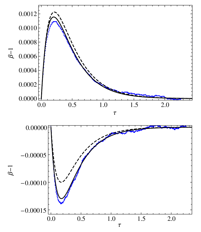
Figure 1.11: Emergence of anomalous Kovacs response in a uniformly heated granular gas. Specifically, $\beta=\sqrt{T_{s}/T}$, where $T_{s}$ is the steady value of the temperature, and $\tau$ measures time in the number of collisions per particle. Therefore, a maximum in the temperature corresponds to a minimum in $\beta$ and vice versa. (Top) Highly inelastic case (restitution coefficient $\alpha=0.3$), for which the anomalous Kovacs response is clearly observed. (Bottom) Inelasticity is decreased ($\alpha=0.8$, closer to the elastic case $\alpha=1$) and the Kovacs response becomes normal. The crossover from normal to anomalous response takes place at $\alpha=1/\sqrt{2}$; a detailed discussion can be found in [112], from which the figure is taken.

Kovacs-like behavior has also been reported in other, more complex, athermal systems. This is the case of disordered mechanical systems [118] and active matter [119]. In the latter, a “giant” Kovacs hump has been observed, with the numerically observed maximum being much larger than the one predicted by the extrapolation of the linear response expression (1.20) to the considered nonlinear protocol. Moreover, an alternative derivation of (1.20) has been provided in the supplemental material of [119]. This derivation holds for athermal systems, since it does not make use of either the explicit form of the probability distribution or the relationship between response functions and time correlations at the steady state. Nevertheless, it is restricted to discrete-time dynamics at the macroscopic (average) level of description. In chapter 6, we proceed to generalize these results for continuous time dynamics and also for the mesoscopic level of description. Therein, the dynamics is governed by a master equation for the probability distribution function, from which the macroscopic description can be obtained in the appropriate limit.

1.2.4 Summary of part II

As advanced above, part II is devoted to the thorough analysis of a lattice model that attempts to catch the essential phenomenology of the shear modes of granular fluids.

In each chapter, we explore different aspects of the model. We start by introducing the model in chapter 4. Therein, we focus on the continuous hydrodynamic-like limit that, to the lowest order, leads to equations completely analogous to those in (1.13). In that limit, we study different relevant physical states. Specifically, we analyze the Homogeneous Cooling State and the Uniform Shear Flow state through its one-particle velocity distribution. We also go beyond the aforementioned lowest order analysis in two ways: (i) looking into the behavior of the fluctuating fields and (ii) solving exactly the Homogeneous Cooling State on the lattice.

In chapter 5, we turn our attention to the stability of the NESS of this model system. Not only have we proven the global stability of a quite general family of states, but also clarified the inadequacy of $H_{B}$, given by (1.16), as a Lyapunov functional. We finish the chapter with a rigorous proof of an $H$-theorem. To the best of our knowledge, our result constitutes the first proof, even in simple models, of an $H$-theorem within the context of systems with nonconservative interactions.

Finally, chapter 6 is devoted to the analysis of Kovacs-like memory effects. We develop a general theoretical framework for the linear response analysis in athermal systems, starting from either the master equation for the probability distribution function (mesoscopic description) or the evolution equations for the macroscopic moments (macroscopic description). Our results are particularized for a variant of our lattice model of granular gas, and they show an excellent agreement with simulations. Although we test the theory in our specific model, it is worth noting the quite broad range of physical systems that our developed theoretical framework can be directly applied to.

Appendices B-F deal with some technicalities that are skipped within the main text of this part of the thesis.

Part I Predicting the unfolding pathway of modular systems with toy models

Chapter 2 The basics of modelling modular systems

Over the course of this first part of the thesis, we study in depth a simple model of elasticity for biomolecules. This model, introduced by Guardiani et al. [17] for simulation purposes, lacked a thorough theoretical analysis.

Herein, we specifically look for a theory capable of predicting the unfolding pathway in modular biomolecule submitted to mechanical pulling. We expect that this theory could also explain the unfolding pathway observed in experiments [16] and simulations [17] of the maltose binding protein. As described in the introduction chapter, the unfolding pathway depends on the pulling velocity: at very low pulling rates, it is the weakest unit that unfolds first, while at higher rates the first unit to unravel is the pulled one.

This chapter is dedicated to the development of the aforementioned theory and its plan is detailed below. We start by introducing the basics of the model in section 2.1. The system dynamical response to mechanical pulling is obtained by means of a perturbative approach in section 2.2. Section 2.3 is devoted to the obtention of the solution of the dynamical equations, which allows us to study the emergence of a set of critical velocities at which the unfolding pathway changes. Section 2.4 is dedicated to the comparison of the theoretical predictions with numerical results of the model equations. We seek more realistic variants of the model in section 2.5. Finally, we propose a possible experiment for testing our theory in section 2.6.

2.1 The model fundamentals

Let us consider a certain modular biomolecule comprising $N$ modules. The paradigmatic example is a polyprotein composed of $N$, possibly different, modules. Notwithstanding, we may also be considering a protein domain with $N$ unfoldons. From now on, we will refer to these modules or unfoldons, indistinctly, as modules or units. When the system is submitted to an external force $F$, the simplest description is to portray it as a one-dimensional chain in the direction of the force. We denote the end-to-end extension of the $i$-th unit by $x_{i}$. In a real AFM experiment, the molecule is attached as a whole to the AFM device and stretched. Following Guardiani et al. [17], we model this system with a sequence of nonlinear bonds, as in figure 2.1. Therein, the endpoints of the $i$-th unit are denoted by $q_{i-1}$ and $q_{i}$, so that its extension $x_{i}$ is

$$x_{i}=q_{i}-q_{i-1},\quad i=1,\ldots,N.$$ (2.1)

In this basic model, we consider that the left end of the first unit is fixed, that is, $q_{0}=0$ for all times.

We assume that the inertia terms can be neglected and the evolution of the system follows the coupled overdamped Langevin equations

$$\gamma\dot{q}_{i}=-\frac{\partial}{\partial q_{i}}A(q_{0},\ldots,q_{N})+\eta_{i},$$ (2.2)

in which $\eta_{i}$ are Gaussian white noise terms. They verify

$$\langle\eta_{i}(t)\rangle=0,\quad\langle\eta_{i}(t)\eta_{j}(t^{\prime})\rangle=2\gamma k_{B}T\delta_{ij}\delta(t-t^{\prime}),$$ (2.3)

with $\gamma$ being the friction coefficient of each unit (the same for all), $T$ the temperature of the fluid in which the protein is immersed, and $k_{B}$ the Boltzmann constant. The global free energy function of the system is

$$A(q_{0},\ldots,q_{N})=\sum_{i=1}^{N}a_{i}(q_{i}-q_{i-1})+a_{p}(q_{N})\,.$$ (2.4)

In (2.4), $a_{p}(q_{N})$ is the contribution to the free energy introduced by the force control or length control device, see below, while $a_{i}(x_{i})$ is the contribution to $A$ stemming from the $i$-th unit, which is only function of its own extension $x_{i}$.

The total length of the system is given by

$$\sum_{i=1}^{N}x_{i}=q_{N}.$$ (2.5)

In force control experiments, the applied force $F$ is a given function of time, whereas in length control experiments the device (portrayed by the spring in figure 2.1) tries to keep the total length $q_{N}$ equal to the desired value $L$, also a certain function of time. The corresponding contributions to the free energy are

$$a_{p}(q_{N})=-Fq_{N},\qquad\text{force control},$$ (2.6a)

$$a_{p}(q_{N})=\frac{1}{2}k_{c}(q_{N}-L)^{2},\qquad\text{length control},$$ (2.6b)

in which $k_{c}$ stands for the stiffness of the length control device. The length is perfectly controlled in the limit $k_{c}\to\infty$, when $q_{N}=L$ for all times. For the sake of a common notation, we have not used different letters for Helmholtz or Gibbs free energies. It has to be understood that, on the one hand, introducing (2.6a) in (2.4), we obtain a Gibbs free energy. On the other hand, if we use (2.6b) in (2.4), and the limit $k_{c}\to\infty$ (taking into account that $a_{p}\to 0$ since the force $k_{c}(L-q_{n})$ goes to a constant Lagrange multiplier), the result is a Helmholtz free energy whose minimum, restrained to the total length constraint, gives the equilibrium configuration of the system.

An apparently similar system, briefly discussed in section 1.1.2, in which each module of the chain follows the Langevin equation $\gamma\dot{x}_{i}=-\partial A/\partial x_{i}+\eta_{i}$, has been analyzed in the literature [40, 41]. In this approach, the modules are completely independent in force control experiments, the global free energy is the sum of individual ones and, because of this, Langevin equations completely neglect the spatial structure of the chain. While this simplifying assumption poses no problem for the characterization of the force-extension curves in [41], it is not suited for the investigation of the unfolding pathway. In this context, the spatial structure plays an essential role. The spatial structure of biomolecules can be described in quite a realistic way by using the framework proposed by Hummer and Szabo several years ago [120], but our simplified picture in figure 2.1 makes an analytical approach feasible.

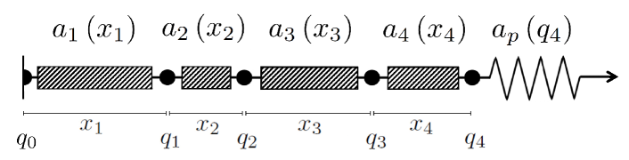
Figure 2.1: Sketch of the basic model for a protein with four units. Each unit is depicted by a rectangle with nonharmonic free energy $a_{i}(x_{i})$. The beads mark the coordinates $q_{i}$ of their endpoints, so that the $i$-th unit’s extension $x_{i}=q_{i}-q_{i-1}$ (by definition, $q_{0}=0$). Finally, the spring represents the device attached to the pulled end $q_{4}$, which controls either the applied force (force control) or the end-to-end distance $q_{4}$ (length control). The device contribution to the free energy is $a_{p}(q_{4})$, see (2.4) and (2.6).

Now, we look into the unfolding pathway of this system. As the evolution equations are stochastic, this pathway may vary from one trajectory of the dynamics to another. Nevertheless, in many experiments [17, 43, 16] a quite well-defined pathway is observed, which suggests that thermal fluctuations do not play an important part in its determination. Physically, this means that the free energy barrier separating the unfolded and folded conformations at coexistence—that is, at the critical force, see below—is expected to be much larger than the typical energy $k_{B}T$ for thermal fluctuations. Therefore, we expect the thermal noise terms in our Langevin equations to be negligible and, consequently, they will be dropped in the remainder of our theoretical approach. Of course, if the unfolding barrier for a given biomolecule were only a few $k_{B}T$s, the thermal noise terms in the Langevin equations could not be neglected and our theoretical approach would have to be changed.

In order to undertake a theoretical analysis of the stretching dynamics, we introduce one further simplification of the problem. We consider that the device controlling the length is perfectly stiff, thus the total length $q_{N}=L$ does not fluctuate. We expect this assumption to have little impact on the unfolding pathway: otherwise, the latter would be more a property of the length control device than of the chain. In fact, we show in section 2.4.2 that the unfolding order is not affected by this simplification. For perfect length control, the mathematical problem is identical to that of the force control situation, but now the force $F$ is an unknown (Lagrange multiplier) that must be calculated at the end by imposing the constraint $q_{N}=\sum_{i}x_{i}=L$. Therefore, the extensions $x_{i}$’s obey the deterministic equations

$$\gamma\dot{x}_{1}= -a^{\prime}_{1}(x_{1})+a^{\prime}_{2}(x_{2}),$$ (2.7a)

$$\gamma\dot{x}_{i}= -2a^{\prime}_{i}(x_{i})+a^{\prime}_{i+1}(x_{i+1})+a^{\prime}_{i-1}(x_{i-1}),\quad 1<i<N,$$ (2.7b)

$$\gamma\dot{x}_{N}= -2a^{\prime}_{N}(x_{N})+a^{\prime}_{N-1}(x_{N-1})+F,$$ (2.7c)

$$F= \,\,\gamma v_{p}+a^{\prime}_{N}(x_{N}).$$ (2.7d)

We have introduced the pulling speed

$$v_{p}\equiv\dot{L},$$ (2.8)

which is usually time independent.

We assume that $a_{i}(x_{i})$ allows for bistability in a certain range of the external force $F$, in the sense that $a_{i}(x_{i})-Fx_{i}$ is a double-well potential with two minima, see figure 2.2. Therefore, in that force range, each unit may be either folded, if $x_{i}$ is in the well corresponding to the minimum with the smallest extension, or unfolded, when $x_{i}$ belongs to the well with the largest extension. If the length is kept constant ($v_{p}=0$), there is an equilibrium solution of (2.7),

$$a^{\prime}_{1}(x_{1}^{\text{st}})=a^{\prime}_{2}(x_{2}^{\text{st}})=\cdots=a^{\prime}_{N}(x_{N}^{\text{st}})=F^{\text{st}},$$ (2.9)

and $F^{\text{st}}$ is calculated with the constraint $\sum_{i}x_{i}^{\text{st}}=L$. This solution is stable as long as $a^{\prime\prime}_{i}(x_{i}^{\text{st}})>0$ for all $i$.

If all the units are identical, $a_{i}(x)=a(x)$, the metastability regions of each module—the range of forces for which the equation $a^{\prime}_{i}(x)=F$ has several solutions—coincide.

Therefore, as briefly introduced in section 1.1.2, we obtain stationary branches corresponding to $J$ unfolded units and $N-J$ folded units that have been analyzed in detail in [41, 39]. If all the modules are not identical, the metastability regions do not perfectly overlap since the units are not equally strong: the weakest one is that for which the equation $a^{\prime}_{i}(x)=F$ ceases to have multiple solutions at a smaller force value.

It is important to note that if we change all the forces $a^{\prime}_{i}(x_{i})$ to $\tilde{a}^{\prime}_{i}(x_{i})=a^{\prime}_{i}(x_{i})-F_{0}$ and $F$ to $\varphi=F-F_{0}$, we have the same system (2.7) but with $\tilde{a}^{\prime}_{i}$ and $\varphi$ instead of $a^{\prime}_{i}$ and $F$, respectively. Then, we may use the free energies for any common value of the force $F_{0}$ and interpret the Lagrange multiplier as the excess force from this value to be applied to the system. A similar result is also found if the length is controlled by using a device with a finite value of the stiffness $k_{c}$. A constant force only shifts the equilibrium point of a harmonic oscillator: $(q_{N}-L)$ must be substituted by $(q_{N}-L-F_{0}/k_{c})$.

2.2 Pulling the system: perturbative solution

We write the $i$-th unit’s free energy as

$$a_{i}(x)=a(x)+\xi\,\delta a_{i}(x),$$ (2.10)

in which $a(x)$ is the “main” part, common to all the units, and $\xi\delta a_{i}(x)$ represents the separation from this main contribution. If all the units are perfectly identical, $a_{i}(x)=a(x)$ for all $i$ or, equivalently, $\delta a_{i}(x)=0$. In principle, in an actual experiment, the splitting of the free energy in (2.10) can be done if the free energy $a_{i}$ of each unit is known: we may define the common part as the “average” free energy over all the units, $a(x)\equiv\overline{a}(x)\equiv N^{-1}\sum_{i=1}^{N}a_{i}(x)$, and $\xi\delta a_{i}(x)\equiv a_{i}(x)-\overline{a}(x)$. From a physical point of view, the dimensionless parameter $\xi>0$ measures the importance of the heterogeneity in the free energies. Our theory could be applied to a situation in which the free energy deviations $\delta a_{i}$ were stochastic and followed a certain probability distribution, for instance to represent the slight differences among very similar units, as done in [41] to analyze the force-extension curves. Also the forces $a^{\prime}_{i}(x)$ in the evolution equations are split as

$$a^{\prime}_{i}(x)=a^{\prime}(x)+\xi\,\delta\!f_{i}(x),\quad\delta\!f_{i}(x)\equiv\delta a^{\prime}_{i}(x).$$ (2.11)

As already noted above, we can use the free energies for any common value of the force $F_{0}$, and interpret $F$ as the extra applied force from this value. In what follows, we consider the main part $a(x)$ with two, equally deep, minima corresponding to the folded (F) and unfolded (U) configurations. Therefore, our “origin of force” $F_{0}$ corresponds to the critical force for the main, common, contribution $a$ to the units’ free energies. Figure 2.2 presents a qualitative picture of the free energy and its derivative. The two minima correspond to lengths $\ell_{F}$ and $\ell_{U}$, with $\ell_{F}<\ell_{U}$. Also the point $\ell_{b}$ at which $a^{\prime\prime}(\ell_{b})=0$ is marked.

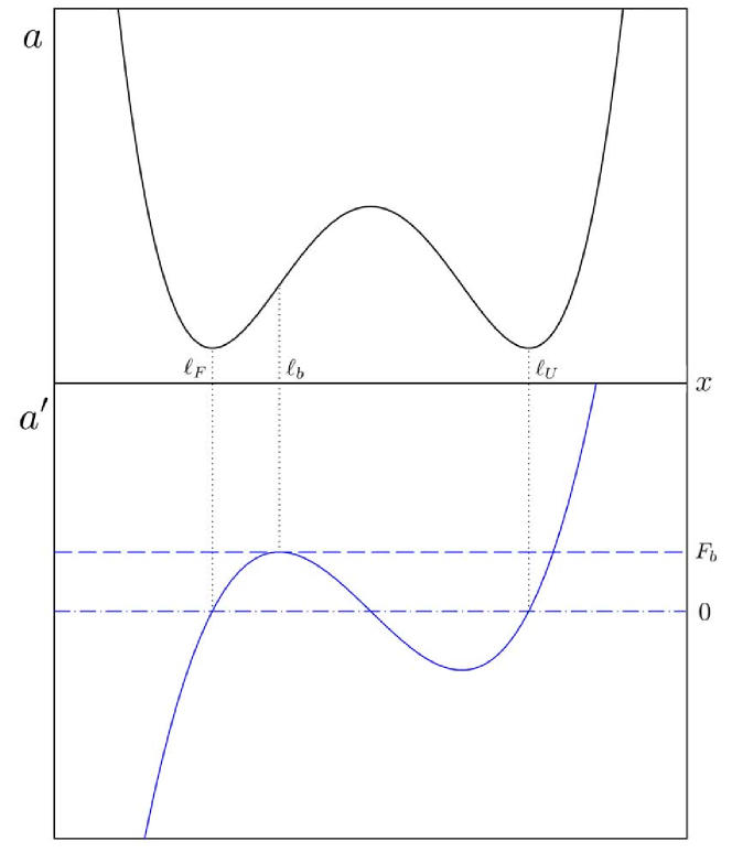
Figure 2.2: Qualitative behavior of the main contribution to the free energy $a(x)$ (top) and its associated force $a^{\prime}(x)$ (bottom) as functions of the extension. Specifically, the plots correspond to the critical force, for which the two minima of the free energy are equally deep. The values of the lengths at the folded and unfolded minima are $\ell_{F}$ and $\ell_{U}$, respectively. The threshold length $\ell_{b}$ stands for the length at the limit of stability, with $F_{b}$ being the corresponding force.

It is the condition $a^{\prime\prime}(\ell_{b})=0$ that essentially determines the stability threshold, as it provides the limit force $F_{b}=a^{\prime}(\ell_{b})>0$ at which the folded basin ceases to exist for the “main” potential. In the deterministic approximation considered here, thermal fluctuations are neglected and, for $F<F_{b}$, the folded unit cannot jump over the free energy barrier hindering its unfolding: it has to wait until, at $F=F_{b}$, the only possible extension is that of the unfolded basin. Of course, neglecting thermal noise restricts in some way the range of applicability of our results, see section 2.3 for a more detailed discussion and also the numerical section 2.4.2.

Keeping the above discussion in mind, now we analyze the limit of stability of the different units. The asymmetry correction $\delta f_{i}$ shifts the threshold force for the different units and the extension $x_{i,b}$ at which the $i$-th unit loses its stability is obtained by solving the equation $a^{\prime\prime}_{i}(x_{i,b})=a^{\prime\prime}(x_{i,b})+\xi\delta f^{\prime}_{i}(x_{i,b})=0$. Linearizing in both the displacement $x_{i,b}-\ell_{b}$ and $\xi$ one gets

$$a^{\prime\prime}(\ell_{b})+a^{\prime\prime\prime}(\ell_{b})(x_{i,b}-\ell_{b})+\xi\delta f^{\prime}_{i}(\ell_{b})=0.$$ (2.12)

Noting that $a^{\prime\prime}(\ell_{b})=0$, we obtain

$$x_{i,b}=\ell_{b}-\xi\,\frac{\delta f^{\prime}_{i}(\ell_{b})}{a^{\prime\prime\prime}(\ell_{b})}.$$ (2.13)

The corresponding force is

$$F_{i,b}\equiv a^{\prime}_{i}(x_{i,b})=F_{b}+\xi\,\delta\!f_{i}(\ell_{b}),$$ (2.14)

in which we have consistently dropped terms of the order of $\xi^{2}$. Then, units with $\delta\!f_{i}(\ell_{b})<0$ ($\delta\!f_{i}(\ell_{b})>0$) are weaker (stronger) than average. See appendix A for more details.

When the system is pulled, the total length of the system $L$ has been shown to be a good reaction coordinate [121] and, on physical grounds, it is reasonable to use $L$ to measure time. Therefore, we write the evolution equations (2.7) as

$$\gamma v_{p}\frac{dx_{1}}{dL}= -a^{\prime}(x_{1})+a^{\prime}(x_{2})+\xi[-\delta f_{1}(x_{1})+\delta\!f_{2}(x_{2})],$$ (2.15a)

$$\gamma v_{p}\frac{dx_{i}}{dL}= -2a^{\prime}(x_{i})+a^{\prime}(x_{i+1})+a^{\prime}(x_{i-1})+\xi[-2\delta\!f_{i}(x_{i})+\delta\!f_{i+1}(x_{i+1})+\delta f_{i-1}(x_{i-1})],$$

$$\qquad\qquad\qquad\qquad\qquad\qquad\qquad\qquad\qquad\qquad\qquad\qquad\qquad\qquad 1<i<N,$$ (2.15b)

$$\gamma v_{p}\frac{dx_{N}}{dL}= -2a^{\prime}(x_{N})+a^{\prime}(x_{N-1})+F+\xi[-2\delta f_{N}(x_{N})+\delta\!f_{N-1}(x_{N-1})],$$ (2.15c)

$$F= \,\,\gamma v_{p}+a^{\prime}(x_{N})+\xi\,\delta\!f_{N}(x_{N}).$$ (2.15d)

Moreover, this change of variable makes the pulling speed $v_{p}$ appear explicitly in the equations, allowing us to consider $v_{p}$ as a perturbation parameter for slow enough pulling processes.

Now, we consider a system such that (i) the asymmetry in the free energies is small and (ii) it is slowly pulled. Equations (2.15) are solved by means of a perturbative expansion in powers of the pulling velocity $v_{p}$ and the disorder parameter $\xi$, that is,

$$x_{i}(L)= \,\,x_{i}^{(0)}(L)+\xi\delta x_{i}(L)+v_{p}\Delta x_{i}(L),$$ (2.16a)

$$F(L)= \,\,F^{(0)}(L)+\xi\delta F(L)+v_{p}\Delta F(L),$$ (2.16b)

up to the linear order in both $v_{p}$ and $\xi$.

The zero-th (lowest) order corresponds to the chain of identical units, $\xi=0$, with a given constant length $L$, $v_{p}=0$. Namely, $x_{i}^{(0)}$ and $F^{(0)}$ obey the equations

$$0= -a^{\prime}(x_{1}^{(0)})+a^{\prime}(x_{2}^{(0)}),$$ (2.17a)

$$0= -2a^{\prime}(x_{i}^{(0)})+a^{\prime}(x_{i+1}^{(0)})+a^{\prime}(x_{i-1}^{(0)}),\quad 1<i<N,$$ (2.17b)

$$0= -2a^{\prime}(x_{N}^{(0)})+a^{\prime}(x_{N-1}^{(0)})+F^{(0)},$$ (2.17c)

$$F^{(0)}= \,\,a^{\prime}(x_{N}^{(0)}),$$ (2.17d)

which have the straightforward solution

$$a^{\prime}(x_{i}^{(0)})=F^{(0)}.$$ (2.18)

The force is equally distributed among all the units of the chain in equilibrium, as expected.

If we start the pulling process from a configuration in which all the units are folded and the force is outside the metastability region, that is, the usual situation, the units extensions and the applied force are

$$x_{i}^{(0)}=\ell\equiv\frac{L}{N},\quad\forall i,\qquad F^{(0)}=a^{\prime}(\ell),$$ (2.19)

to the lowest order. To calculate the linear corrections in $\xi$ and $v_{p}$, we have to substitute (2.16) and (2.19) into (2.15), and equate terms proportional to $\xi$ and $v_{p}$, respectively. This is done below in two separate sections: first, for the asymmetry contribution $\delta x_{i}$, and second, for the “kinetic” contribution $\Delta x_{i}$.

2.2.1 Asymmetry term

All the modules are not characterized by the same free energy. Here, we calculate the first order correction introduced by this “asymmetry” in the modules. The asymmetry corrections $\delta x_{i}$ obey the system of equations

$$\delta x_{2}-\delta x_{1}= \,\,\frac{\delta\!f_{1}(\ell)-\delta\!f_{2}(\ell)}{a^{\prime\prime}(\ell)},$$ (2.20a)

$$\delta x_{i+1}+\delta x_{i-1}-2\delta x_{i}= \,\,\frac{2\delta\!f_{i}(\ell)-\delta\!f_{i+1}(\ell)-\delta\!f_{i-1}(\ell)}{a^{\prime\prime}(\ell)},\quad 1<i<N,$$ (2.20b)

$$\delta x_{N-1}-2\delta x_{N}= \,\,\frac{2\delta\!f_{N}(\ell)-\delta\!f_{N-1}(\ell)-\delta F}{a^{\prime\prime}(\ell)},$$ (2.20c)

$$\delta F= \,\,a^{\prime\prime}(\ell)\delta x_{N}+\delta\!f_{N}(\ell),$$ (2.20d)

which is linear in the $\delta x_{i}$’s, and thus can be analytically solved. Note that our expansion breaks down when $a^{\prime\prime}(\ell)=0$. This was expected, since the stationary branch with all the modules folded is unstable when $a^{\prime\prime}_{i}$ becomes negative for some unit $i$, and to the lowest order this takes place when $a^{\prime\prime}(\ell)=0$.

The solution of (2.20) is obtained by standard methods for solving difference equations [122], with the result

$$\delta x_{i}=\frac{\overline{\delta\!f}(\ell)-\delta\!f_{i}(\ell)}{a^{\prime\prime}(\ell)},\;\forall i,\quad\delta F=\overline{\delta\!f}(\ell)=\frac{1}{N}\sum_{i=1}^{N}\delta f_{i}(\ell).$$ (2.21)

Interestingly, the force is homogeneous across the chain, since to first order in $\xi$ we have that

$$a^{\prime}_{i}(x_{i})=a^{\prime}(x_{i}^{(0)})+\xi[a^{\prime\prime}(x_{i}^{(0)})\delta x_{i}+\delta\!f_{i}(x_{i}^{(0)})]=a^{\prime}(\ell)+\xi\overline{\delta\!f}(\ell)=F^{(0)}+\xi\delta F,$$ (2.22)

where we have made use of (2.11), (2.19) and (2.21). Equation (2.22) is nothing but the stationary solution (2.9), up to first order in the disorder. If the zero-th order free energy were the average of the $a_{i}$’s, no correction for the Lagrange multiplier (applied force) would appear to the first order. This is logical, up to the first order, the force expression coincides with the spatial derivative of the average potential, that is, $F^{(0)}+\xi\delta F=a^{\prime}(\ell)+\xi\overline{\delta\!f}(\ell)=\overline{a^{\prime}}(\ell)$. Moreover, (2.21) implies that there are units with $\delta x_{i}>0$ and others with $\delta x_{i}<0$, depending on the sign of $\overline{\delta\!f}(\ell)-\delta\!f_{i}(\ell)$. This is a consequence of the length constraint $\sum_{i}x_{i}^{(0)}=L$ for all times, as given by (2.19), from which $\sum_{i}\delta x_{i}=0$.

Let us remember that we denote by $\ell_{b}$ the value of the extension at which the common main free energy reaches its limit of stability, see figure 2.2. Taking into account only the asymmetry correction, it is the weakest unit that unfolds first: since the most negative $\delta\!f_{i}(\ell)$ leads to the largest positive $\delta x_{i}$ which is the one that verifies the condition $x_{i}=\ell+\xi\delta x_{i}=\ell_{b}$ for the shortest time. For a more detailed discussion, see appendix A. An alternative way of looking at this is to recall that the force corresponding to the limit of stability is smallest for the weakest unit: since the force is homogeneously distributed along the chain, it is the weakest module that first reaches its stability threshold.

2.2.2 Kinetic term

Now we look into the “kinetic” correction that stems from the finite pulling speed $v_{p}$. The zero-th order solution is given by (2.19), so that $dx_{i}^{(0)}/dL=N^{-1}$ for all $i$, and we have

$$\Delta x_{2}-\Delta x_{1}= \,\,\frac{\gamma}{Na^{\prime\prime}(\ell)},$$ (2.23a)

$$\Delta x_{i+1}+\Delta x_{i-1}-2\Delta x_{i}= \,\,\frac{\gamma}{Na^{\prime\prime}(\ell)},\quad 1<i<N,$$ (2.23b)

$$\Delta x_{N-1}-2\Delta x_{N}= \,\,\frac{1}{a^{\prime\prime}(\ell)}\left[\frac{\gamma}{N}-\Delta F\right],$$ (2.23c)

$$\Delta F= \,\,\gamma+a^{\prime\prime}(\ell)\Delta x_{N}.$$ (2.23d)

The solution to this system of linear difference equations is again obtained by employing standard methods [122], with the result

$$\Delta x_{i}= \,\,\frac{\gamma}{2Na^{\prime\prime}(\ell)}\left[i(i-1)-\frac{(N+1)(N-1)}{3}\right],$$ (2.24a)

$$\Delta F= \,\,\frac{(N+1)(2N+1)\gamma}{6N}.$$ (2.24b)

Also, $\sum_{i}\Delta x_{i}=0$ because the zero-th order solution (2.19) gives the total length, $\sum_{i}x_{i}^{(0)}=L$ for all times. Note that (2.24a) is reasonable on intuitive grounds: the kinetic correction $\Delta x_{i}$ increases with $i$ because the last module is the one closer to the pulled end. Therefore, on the basis of only the kinetic correction, it is the last module that would unfold first, since $\Delta x_{N}$ is the largest and the condition $x_{i}=\ell+v_{p}\Delta x_{i}=\ell_{b}$ is first verified for $i=N$.

It is interesting to highlight that the force was equally distributed for the asymmetry correction, as expressed by (2.22), but this is no longer true if we incorporate the kinetic correction. Up to the the first order,

$$a^{\prime}_{i}(x_{i})=a^{\prime}(x_{i}^{(0)}+\xi\delta x_{i}+v_{p}\Delta x_{i})+\xi\delta\!f_{i}(x_{i})\simeq a^{\prime}(\ell)+\xi\overline{\delta\!f}(\ell)+v_{p}a^{\prime\prime}(\ell)\Delta x_{i}.$$ (2.25)

Therefore, the force $a^{\prime}_{i}(x_{i})$ depends on the unit $i$: for all times, it is smaller the further from the pulled unit we are. Again, there is an alternative way of understanding the reason why the last unit would unfold first if we were considering perfectly identical units ($\xi=0$): for any time, it would be the one suffering the largest force, and thus the first to reached their common limit of stability $F_{b}$.

2.3 The critical velocities

If the last unit is not the weakest, there is a competition between the asymmetry and the kinetic corrections. For very low pulling speeds, in the sense that $v_{p}/\xi\to 0$, the term proportional to $v_{p}$ can be neglected and it is the weakest unit (the one with the largest $\delta x_{i}$) that unfolds first, as discussed in section 2.2.1. On the other hand, for very small disorder, in the sense that $\xi/v_{p}\to 0$, the term proportional to $\xi$ is the one to be neglected and it is the last unit (the one with the largest $\Delta x_{i}$) that unfolds first, as also discussed in section 2.2.2. Therefore, different unfolding pathways are expected as the pulling speed is changed.

Collecting all the contributions to the extensions, we have that

$$x_{i}=\ell+\frac{\xi\overline{\delta\!f}(\ell)-v_{p}\gamma\dfrac{N^{2}-1}{6N}}{a^{\prime\prime}(\ell)}+\frac{v_{p}\gamma\dfrac{i(i-1)}{2N}-\xi\delta\!f_{i}(\ell)}{a^{\prime\prime}(\ell)}.$$ (2.26)

We have rearranged the terms in $x_{i}$ in such a way that the first two terms on the rhs are independent of the unit $i$, all the dependence of the length of the module on its position across the chain has been included in the last term. We are expanding the solution in powers of $v_{p}$ around the “static” solution, which is obtained by putting $v_{p}=0$ in (2.26). Thus, the “static” solution corresponds to the stationary one the system would reach if we kept the total length constant and equal to its instantaneous value at the considered time. It is essential to realize that (2.26) is only valid for very slow pulling, as long as the corrections to the “static” solution are small, and this is the reason why the limit of stability is basically unchanged as compared to the static case. In order to be more precise, we refer to this kind of very slow pulling as adiabatic pulling. One of our main results is that, even for the case of adiabatic pulling, there appear different unfolding pathways depending on the value of the pulling speed.

In the adiabatic limit we are considering here, the pulling process has to be slow enough to make the system move very close to the stationary force-length branches, but not so slow to give the system enough time to escape from the folded basin by thermal activation. As discussed in [41], there is an interplay between the pulling velocity and thermal fluctuations. For very slow pulling velocities, the system has enough time to surpass the energy barrier separating the two minima, which leads to the typical logarithmic dependence of the “unfolding force” $F_{U}$ on the pulling speed, specifically $F_{U}\propto(\ln v_{p})^{c}$ [123, 124]. The parameter $c$ is of the order of unity, and its particular value depends on the specific shape of the potential (linear-cubic, cuspid-like, …) considered [124]. On the other hand, as already argued at the beginning of section 2.2, for adiabatic pulling, the units unfold not because they are able to surpass the free energy barrier but because the folded state ceases to exist at the force $F_{b}$ corresponding to the upper limit of the metastability region. Therefore, our predictions are expected to be valid in an intermediate range of velocities: high enough to avoid thermal activation, but low enough to allow for a perturbative analysis of the dynamical equations.

The unit that unfolds first is the one for which $x_{i}=\ell_{b}$ for the shortest time. In light of the above, it is natural to investigate whether it is possible to determine which module is the first to unfold for a given pulling speed. To put it another way, we would like to calculate the “critical” velocities separating velocity intervals inside which a specific module unfolds first. Let us assume that, for a given pulling speed $v_{p}$, it is the $i$-th module that unfolds first. All the modules $j$ to its left, that is, with $j<i$, will not open first if the pulling velocity is further increased because the difference between the kinetic corrections $\Delta x_{i}-\Delta x_{j}$ increases with $v_{p}$. Therefore, the first module $j$ that unfolds when the velocity surpasses some critical value is always to its right. More specifically, velocity $v^{i}(j)$ for which each couple of modules $(i,j)$, $j>i$, reach simultaneously the stability threshold verifies

$$x_{i}(\ell_{c})=x_{j}(\ell_{c})=\ell_{b},$$ (2.27)

which yields both the value of $\ell_{c}$ (or time $t_{c}$) at which the stability threshold is reached and the relationship between $v_{p}$ and $\xi$. Equations (2.26) and (2.27) imply that

$$-\xi\delta f_{i}(\ell_{c})+\gamma v^{i}(j)\frac{i(i-i)}{2N}=-\xi\delta\!f_{j}(\ell_{c})+\gamma v^{i}(j)\frac{j(j-1)}{2N}.$$ (2.28)

We already know that the length corresponding to the limit of stability is very close to the threshold length $\ell_{b}$, its distance thereto being of the order of $\sqrt{\xi}$, as shown in appendix A. Therefore, to the lowest order, $\ell_{c}$ can be approximated by $\ell_{b}$ and we get

$$\frac{\gamma v^{i}(j)}{\xi}=\frac{2N[\delta\!f_{j}(\ell_{b})-\delta\!f_{i}(\ell_{b})]}{j(j-1)-i(i-1)},\quad j>i.$$ (2.29)

Clearly, the minimum of these velocities $v^{i}(j)$ is the one that matters. Let us denote by $j^{(i)}_{\text{min}}$ the position of the module for which $v^{i}(j)$ reaches its minimum value $v_{\text{min}}^{i}$,

$$v_{\text{min}}^{i}=v^{i}(j^{(i)}_{\text{min}})=\min_{j}v^{i}(j)$$ (2.30)

for $v_{p}$ just below $v_{\text{min}}^{i}$, it is the $i$-th module that unfolds first, but for $v_{p}$ just above $v_{\text{min}}^{i}$, it is the $j^{(i)}_{\text{min}}$-th module that unfolds first. Let us denote the weakest module by $\alpha_{1}$, that is, $\delta\!f_{i}(\ell_{b})$ is smallest for $i=\alpha_{1}$. If $v_{p}$ is smaller than $v_{\text{min}}^{\alpha_{1}}$, the first unit to reach the stability limit is the weakest one. Then, we rename the latter velocity $v_{c}^{(1)}$, that is,

$$v_{c}^{(1)}=v_{\text{min}}^{\alpha_{1}},\quad\delta\!f_{\alpha_{1}}(\ell_{b})=\min_{i}\delta\!f_{i}(\ell_{b}),$$ (2.31)

because it is the first one of a (possible) series of critical velocities separating different unfolding pathways, as detailed below.

Let us denote by $\alpha_{2}$ the module which unfolds first in the “second” velocity region, $v_{p}$ just above $v_{c}^{(1)}$, that is, $\alpha_{2}=j_{\text{min}}^{(\alpha_{1})}$. This unit ceases to be the first to unfold for the velocity

$$v_{c}^{(2)}=v_{\text{min}}^{\alpha_{2}}.$$ (2.32)

The successive changes on the unfolding pathway take place at the critical velocities

$$v_{c}^{(k)}=v_{\min}^{\alpha_{k}},$$ (2.33)

at which $\alpha_{k+1}=j_{\text{min}}^{(\alpha_{k})}$. This succession ends when $\alpha_{k+1}=N$: in that case, for $v_{p}>v^{(k)}_{c}$, the first unit to unfold is always the pulled one. This upper critical velocity $v_{c}^{\text{end}}$ can be computed in a more direct way,

$$v_{c}^{\text{end}}=\max_{j}v^{j}(N).$$ (2.34)

Consistency of the theory requires that $v_{c}^{(k+1)}>v_{c}^{(k)}$. This can be proved right away. The consistency condition implies that

$$\delta\!f_{\alpha_{k+2}}(\ell_{b})>\frac{\delta\!f_{\alpha_{k+1}}(\ell_{b})(\nu_{k+2}-\nu_{k})-\delta\!f_{\alpha_{k}}(\ell_{b})(\nu_{k+2}-\nu_{k+1})}{\nu_{k+1}-\nu_{k}},$$ (2.35)

in which $\nu_{k}=\alpha_{k}(\alpha_{k}-1)$. Due to (2.33), $\alpha_{k+1}$ minimizes $v^{\alpha_{k}}(j)$. Therefore, in particular, $v^{\alpha_{k}}(\alpha_{k+1})<v^{\alpha_{k}}(\alpha_{k+2})$, which is readily shown to be equivalent to (2.35) and proves the inequality.

We have a trivial case for $\alpha_{1}=N$, when the pulled unit is precisely the weakest and it is always the first to unfold for any pulling speed. The simplest nontrivial case appears when all the modules have the same free energy with the exception of the weakest, and $\alpha_{1}\neq N$, (2.29), (2.31) and (2.34) reduce to

$$\frac{\gamma v^{(1)}_{c}}{\xi}=\frac{\gamma v^{\text{end}}_{c}}{\xi}=\frac{2N[\delta\!f_{N}(\ell_{b})-\delta\!f_{\alpha_{1}}(\ell_{b})]}{N(N-1)-\alpha_{1}(\alpha_{1}-1)}.$$ (2.36)

Note that the situation is quite simple, since there exist a single critical velocity $v_{c}=v_{c}^{(1)}=v_{c}^{\text{end}}$. For $v_{p}<v_{c}$ the weakest module unfolds first whereas for $v_{p}>v_{c}$ the last one unfolds first. If more units have different free energies, the situation may be more complex, as shown in the previous paragraph. There appear intermediate critical velocities, which define pulling speed windows where neither the weakest unit nor the last one is the first to unfold. In order to obtain these regions, we need to recursively evaluate (2.33).

2.4 Comparing our theory with simulations

2.4.1 Free energies of the units: shape and physical parameters

Different shapes for the double-well potentials have been considered in the literature. They can be classified in, mainly, two different classes: simple Landau-like quartic potentials which are employed to understand the basic mechanisms underlying the observed behaviors [17, 41, 39], and more complex realistic potentials, when the aim is obtaining a more detailed, closer to quantitative, description of the experiments [40, 41, 126, 127].

For the simplest modeling of a double well, we use a quartic potential $a_{q}(x)$

$$a_{q}(x)=\frac{\varepsilon}{4}\left[\left(x-\sigma\right)^{2}-\alpha^{2}\right]^{2}.$$ (2.37)

The physical meaning of the parameters are straightforward: $\varepsilon$ scales the shape of the potential, $x=\sigma$ gives the position of the maximum of the barrier, whereas the minima are at $x=\sigma\pm\alpha$. This simple dependence allows us to compute analytically the borders of the metastability region, specifically one can obtain the stability threshold

$$\ell_{b}=\sigma-\frac{\alpha}{\sqrt{3}},$$ (2.38)

and the forces within the metastability region fulfill

$$|F|<F_{b}=a^{\prime}(\ell_{b})=\frac{2\sqrt{3}}{9}\varepsilon\alpha^{3}.$$ (2.39)

Below, we use a nondimensional version of this potential. It is done by defining a length scale $[x]$ and a energy scale $\varepsilon[x]^{4}$,

$$a_{q}(x)=\frac{1}{4}\left[\left(x-\sigma\right)^{2}-\alpha^{2}\right]^{2}$$ (2.40)

where we have not used any special notation for the nondimensional variables in order not to clutter our formulae.

The more realistic proposal we use in this work has been put forward by Berkovich et al. some years ago [126, 127]. Therein, the free energy of a module is represented by the sum of a Morse potential, which mimics the enthalpic minimum of the folded state, and a WLC term [29], which accounts for the entropic contribution to the elasticity of the unfolded state. Specifically, Berkovich’s free energy $a_{B}(x)$ is written as

$$a_{B}(x)=U_{0}\left[\left(1-e^{-2b\frac{x-R_{c}}{R_{c}}}\right)^{2}-1\right]+\frac{k_{B}T}{4P}L_{c}\left(\frac{1}{1-\frac{x}{L_{c}}}-1-\frac{x}{L_{c}}+\frac{2x^{2}}{L_{c}^{2}}\right).$$ (2.41)

This shape has shown to be useful for some pulling experiments with actual proteins as titin I27 or ubiquitin [126, 127]. Therein, each parameter has a neat physical interpretation. First, in the WLC part, we recall (see section 1.1.2) that we have: (i) the contour length $L_{c}$, which is the maximum length for the totally extended protein, and (ii) the persistence length $P$, which measures the characteristic length over which the chain is flexible. Both of them, $L_{c}$ and $P$, can be thought in terms of the number of amino acids in the chain. Note that the derivative of the WLC term leads precisely to the force-extension curve given by (1.6), with the identification $L\leftrightarrow x$. Second, for the Morse contribution, we have: (iii) $R_{c}$, which gives the location of the enthalpic minimum and (iv) $U_{0}$ and $b$, which measure the depth and the width (in a nontrivial form) of the folded basin. The explicit function giving the stability threshold $\ell_{b}$ in terms of the parameters in Berkovich’s potential cannot be obtained. However, we can always estimate $\ell_{b}$ numerically, solving $a_{B}^{\prime\prime}(\ell_{b})=0$ for a specific set of parameters.

Once more, we use below nondimensional variables. In order to do so, we define a force scale $[F]$ and take $L_{c}$ as the length unit. Accordingly, dimensionless variables are introduced with the definitions $\mu=U_{0}/(L_{c}[F])$, $\beta=2bL_{c}/R_{c}$, $\rho=R_{c}/L_{c}$, $A=k_{B}TL_{c}/(4PU_{0})$. Thus, the corresponding dimensionless potential reads

$$a_{B}(x)=\mu\!\left\{\left[1-e^{-\beta(x-\rho)}\right]^{2}-1+A\!\left(\frac{1}{1-x}-1-x+2x^{2}\right)\right\}.$$ (2.42)

2.4.2 Numerical results

Here, we check the agreement between our theory and the numerical integration of the evolution equations. First, we discuss the validity of the simplifications introduced in the development of the theory, namely (i) negligible thermal noise and (ii) perfect length control. Second, we look into the critical pulling speed, showing that there appears such a critical speed in the simulations and comparing this numerical value with our theory.

We consider a system composed of $N=4$ units, such as the maltose binding protein [17], see section 1.1.3. First, each unit is assumed to be characterized by a quartic bistable free energy. In reduced variables, the free energies have the form $a_{i}(x)=\epsilon_{i}a(x)$, with $\epsilon_{i}=1$ for $i\neq 1$, $\epsilon_{1}<1$, where $a(x)=a_{q}(x)$ as given by (2.40), with $\sigma=0$ and $\alpha=3$. Here, the value of $\sigma$ is different from the one in [17] ($\sigma=8$). Its only effect is a shift of the origin of the extensions, our choice implies that a positive (negative) sign of the extension corresponds to an unfolded (folded) configuration. The value of the friction coefficient is, also in reduced variables, $\gamma=1$. We use these dimensionless reduced variables to make it easier to compare our results with those in [17].

As stated above, the function (2.40) is one of the simplest, but reasonable, choices to describe the free energy of different unit of the same modular biomolecule. Using the notation introduced in (2.11), we have

$$\delta\!f_{i}(x)=0,\;i\neq 1,\qquad\delta\!f_{1}(x)=-\xi a_{q}^{\prime}(x),$$ (2.43)

with $\xi=1-\epsilon_{1}$. Equations (2.13) and (2.14) give us the limits of stability up to first order in the asymmetry $\xi$,

$$x_{i,b}=\ell_{b},\;\forall i,\quad F_{i,b}=F_{b},\;i\neq 1,\qquad F_{1,b}=(1-\xi_{1})F_{b}.$$ (2.44)

For this simple example, (2.44) is exact. The weakest unit is the first one, because $F_{1,b}$ is the minimum value of the force at the limit of stability. For the values of the parameters we are using, $\ell_{b}=-\alpha/\sqrt{3}=-1.73$ and $F_{b}=a^{\prime}(\ell_{b})=2\sqrt{3}\alpha^{3}/9=10.4$. Since we are writing the free energies for a common given value of the force, all the units have their two minima equally deep at the same force. This assumption is made to keep things simple: the main ingredient for having an unfolding pathway that depends on the pulling speed is to have different values of the forces $F_{i,b}$ at the stability threshold for the different units.

In the case we are considering, the weakest unit is the first one, while the others share the same free energy. This means that we have the simplest scenario for the critical velocity in our theoretical approach: either the weakest (for $v_{p}<v_{c}$) or the last (for $v_{p}>v_{c}$) unit that opens first, as discussed at the end of the section 2.2. Here, (2.36) for $\alpha_{1}=1$ and $N=4$ reduces to

$$\frac{\gamma v_{c}}{\xi}=\frac{2}{3}F_{b}.$$ (2.45)

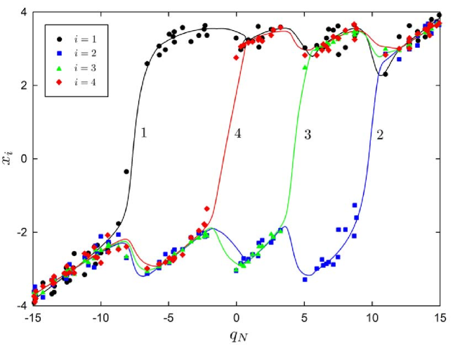
Figure 2.3: Evolution of the units’ extensions as a function of the system length $q_{N}$. The pulling speed is $v_{p}=0.38$ and the length control device has a stiffness $k_{c}=5$. The symbols correspond to a typical realization of the Langevin process (2.2) with $T=1$, whereas the lines correspond to the deterministic (zero noise) approximation.

To start with, we consider the relevance of the noise terms in (2.2). In figure 2.3, we plot the integration of the Langevin equations together with the deterministic approximation [95] for a particular case: the first unit’s free energy corresponds to $\epsilon_{1}=0.8$ ($\xi=0.2$), the stiffness of the length control device is $k_{c}=5$, the temperature is $T=1$, and the pulling speed is $v_{p}=0.38$. For these values of the parameters, taken from [17], the critical velocity in (2.45) is $v_{c}=1.4$; thus we are considering a subcritical velocity, $v_{p}<v_{c}$. Thermal fluctuations are small, which entail that the same unfolding pathway is observed in the deterministic and the majority of the stochastic trajectories.

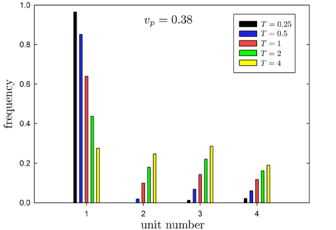
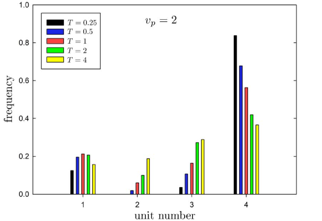
Figure 2.4: First-unfolding frequency for each of the units. These frequencies have been obtained by integrating the Langevin equations with perfect length control, for different values of the temperature. (Top) Numerical frequencies obtained in $1000$ trajectories, for a subcritical pulling speed $v_{p}=0.38<v_{c}$. (Bottom) The same as in the top panel, but for a supercritical pulling speed $v_{p}=2>v_{c}$. As the temperature decreases, the frequency of the deterministic unfolding pathway approaches unity in both cases.

Let us consider in more detail the relevance of thermal noise: from a physical point of view, it may be inferred by looking at the height of the free energy barrier at the critical force in terms of the thermal energy $k_{B}T$. For the values of the parameters we are using, this barrier is around $20k_{B}T$, which explains why thermal noise is basically negligible in figure 2.3. If the temperature is decreased from $T=1$ to $T=0.25$, the barrier is so high, around $80$ times the thermal energy, that essentially all the stochastic trajectories coincide with the deterministic one. On the other hand, if the temperature is increased to $T=4$, the barrier in only a few $k_{B}T$, and we expect that the deterministic approximation ceases to be valid.

In order to further clarify the role played by the temperature, we present figure 2.4. Both panels display bar graphs with the frequencies with which each unit unfolds first in the stochastic trajectories. Specifically, the statistics shown has been obtained with $1000$ trajectories of the Langevin equations (2.2) with perfect length control, and several different values of the temperature. In the top panel, a subcritical velocity $v_{p}=0.38<v_{c}$ is considered, so that the weakest (first) unit is expected to unfold first. In the bottom panel, the numerical data for a supercritical velocity $v_{p}=2>v_{c}$ are shown, for which the pulled (fourth) unit would unfold first. The effect of thermal noise is quite similar in both cases. For the lowest temperature $T=0.25$, the frequency of the deterministic pathway is close to unity and, for the temperature in figure 2.3, $T=1$, its frequency is still very large, clearly larger than any of the others. On the other hand, for the highest temperature, $T=4$, thermal noise is no longer negligible.

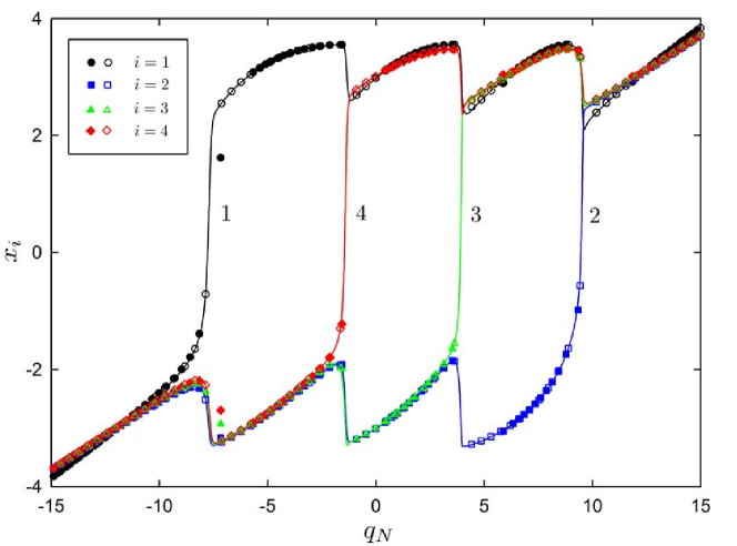
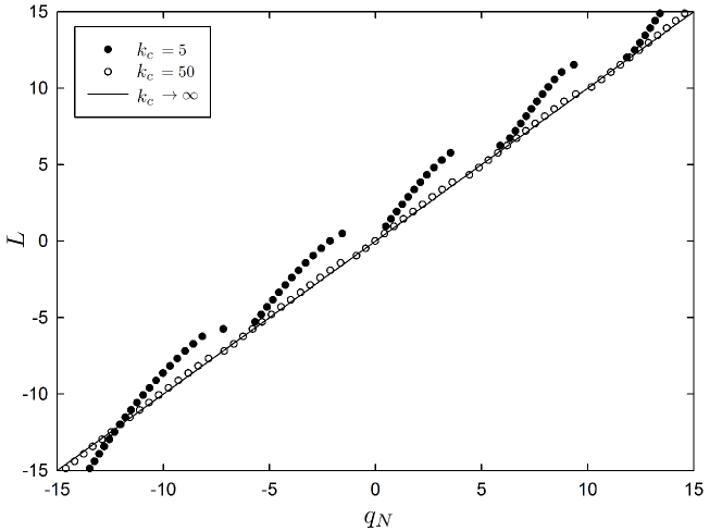
Figure 2.5: (Top) Evolution of the units’ extensions as a function of the system length $q_{N}$. The symbols correspond to the integration of the deterministic equations, for $k_{c}=5$ (filled) and $k_{c}=50$ (empty), whereas the line corresponds to the limit of perfect length control, $k_{c}\to\infty$. The pulling speed is the same as in figure 2.3, that is, $v_{p}=0.38$. (Bottom) Comparison between the desired and actual lengths, $L$ and $q_{N}$. Clearly, the length control improves as $k_{c}$ increases.

In the following, we restrict the analysis to the physically relevant case in which the deterministic approximation gives a good description of the first unfolding event. In figure 2.5 (top panel), we look into the same pulling experiment as before, but now we compare the deterministic evolution of the extensions for two finite values of the stiffness to the $k_{c}\to\infty$ limit. Consistently with our expectations, the unfolding pathway is not affected by this simplification. For the smaller values of $k_{c}$, the length is not perfectly controlled, but the length control improves as $k_{c}$ increases, as seen in the bottom panel. Notwithstanding, the curves in the top panel, which correspond to different values of $k_{c}$, are almost perfectly superimposed when plotted as a function of the real length of the system $q_{N}$ (but not of the desired length $L$). This means that the real length $q_{N}$ is a good reaction coordinate, as already stated in section 2.2.

We have integrated the deterministic approximation (2.7) (zero noise) of the Langevin equations for different values of the pulling speed, and extracted from them the numerical value of the critical velocity as a function of the asymmetry $\xi=1-\epsilon_{1}$. In order to obtain this numerical prediction, we initially set $v_{p}$ equal to the theoretical critical velocity given by (2.45). Then, we recursively shift it by a small amount $\delta v_{p}$, such that $\delta v_{p}/v_{c}=0.0001$, until the pathway changes. We compare the values so obtained to the theoretical expression (2.45), in figure 2.6. We find an excellent agreement for $\xi\lesssim 0.1$, for $\xi>0.1$ there appear some quantitative discrepancies. They stem from two points: (i) the perturbative expansion used for obtaining (2.36) from (2.27) and (ii) the intrinsically approximate character of (2.27), since $\ell_{b}$ gives rigorously the limit of stability only for the static case $v_{p}=0$. Therefore, we have looked for the solution of (2.27) in the numerical integration of the deterministic equations. This is the dashed line in figure 2.6, which substantially improves the agreement between theory and numerics because we have eliminated the deviations arising from point (i) above. In fact, for the case we have studied in the previous figures, which corresponds to a not so small asymmetry $\xi=0.2$, the improved theory gives an almost perfect prediction for the critical velocity. Note that the new numerical estimate of $v_{c}$ by solving (2.27) is always below that given by (2.36). This can be easily understood: since the value $\ell_{c}$ at which $x_{1}$ and $x_{4}$ intersect is lower than $\ell_{b}$, the pulling velocity needed for the crossing is lower than (2.36).

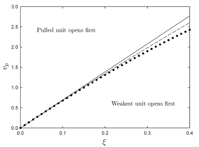
Figure 2.6: Phase diagram for the unfolding pathway in the pulling velocity-asymmetry plane for the quartic potential. Two well-defined regions are observed. These regions are separated by the curve critical velocity $v_{c}$ vs. asymmetry $\xi$ of the first unit. The numerical values for $v_{c}$ (circles) are compared to the theoretical expression (2.45) (solid line). The dashed line corresponds to the alternative approach discussed in the text, which improves the agreement with the numerical results for $\xi>0.1$. Error bars have been omitted because they are smaller than point size.

Now we consider the more realistic Berkovich’s potential, given by (2.41) and (2.42). We take the values of the parameters from [41, 128], namely

$$P=0.4\text{ nm},\quad L_{c}=30\text{ nm},\quad R_{c}=4\text{ nm},\quad b=2,\quad U_{0}=100\text{ pN}\,\text{ nm},$$ (2.46)

and $T=300$ K. Defining the force scale $[F]=100$ pN, the values of the nondimensional parameters in (2.42) are $\mu=0.0333$, $\beta=30$, $\rho=0.133$ and $A=0.776$. In dimensionless variables, $F_{b}=0.527$ ($52.7$ pN) and $\ell_{b}=0.157$ ($4.70$ nm). The relevant time scale is set by the friction coefficient $\gamma$, $[t]=\gamma L_{c}/[F]$. In turn, $\gamma$ is given by the Einstein relation $D=k_{B}T/\gamma$, where $D$ is the diffusion coefficient for tethered proteins in solution. We consider a typical value $D=1500$ nm²/s, also taken from [126], so that $\gamma=0.0028$ pN nm^-1 s.

We consider a system of $4$ units, again with all the units but the first being identical. Then, $a_{i}(x)=a_{B}(x)$, $i\neq 1$, and the first unit is the weakest because $a_{1}(x)=(1-\xi)a_{B}(x)$. The situation is then similar to the one we have already analyzed with the quartic potential (2.40), but there is a difference that should be noted: here, $a_{B}(x)$ is the free energy at zero force, whereas for the quartic potential $a_{q}(x)$ was the free energy at the critical force $F_{0}$ for which the folded and unfolded minima were equally deep. Then, the force here must not be interpreted as the extra force from $F_{0}$, but as the whole force applied to the polyprotein. On the basis of our theory, we expect the simplest situation with only one critical velocity $v_{c}$, below (above) which the weakest unit (the pulled unit) unfolds first. This is also indeed the case in the numerical simulations, and we compare the theoretical and numerical critical velocities in figure 2.7. A very good agreement is found again, up to values of the asymmetry $\xi$ of the order $0.1-0.2$.

The above discussion shows that the validity of the theory presented here is not restricted to simple potentials like the quartic one; on the contrary, it can be confidently applied to situations in which the units are described by realistic potentials. For the typical parameters we are using, the theoretical critical velocity $v_{c}$ for the Berkovich potential equals $1270$nm/s for an asymmetry $\xi=0.1$. The latter can be regarded as a conservative estimate of the largest asymmetries for which our theory gives an almost perfect account of the unfolding pathway. Interestingly, this pulling speed corresponds to the upper range of velocities employed in AFM experiments, for instance see table I of [9]. Therefore, testing our theory in real AFM experiments with modular proteins should be achievable, see also section 2.6.

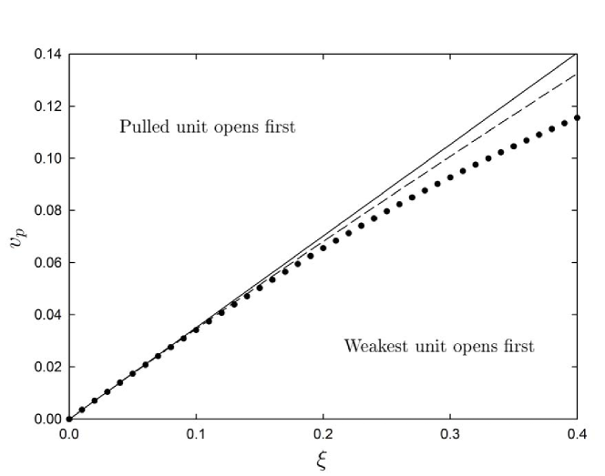
Figure 2.7: Phase diagram for the unfolding pathway in the pulling velocity-asymmetry plane for the Berkovich potential (2.42). As in figure 2.6, there appear two well-defined regions, separated by the curve critical velocity $v_{c}$ vs. asymmetry $\xi$. Numerical values for $v_{c}$ (circles) compare very well with our theoretical prediction (2.36) (solid line). Again, the dashed line corresponds to the alternative approach discussed in the text, which once more improves the agreement theory-simulation as $\xi$ increases.

Finally, we consider a more complex situation, in which more than one unit is different from the rest. Therefore, there may exist more than one critical velocity as discussed in section 2.3. To be concrete, we have considered a system with $4$ units in which $a_{2}(x)=a_{3}(x)=a_{q}(x)$, $a_{1}(x)=(1-\xi)a_{q}(x)$, as before, but the pulled unit free energy is changed to $a_{4}(x)=(1+3\xi/2)a_{q}(x)$. In this situation, we have two different critical velocities: for very low pulling speeds, the weakest unit is the first to unfold, but there appears a velocity window inside which neither the weakest nor the pulled unit is the first to unfold. This stems from the fact that the first and the third unit reach simultaneously the limit of stability for a velocity $v^{1}(3)=4\xi\gamma^{-1}F_{b}/3$ that is smaller than the velocity $v^{1}(4)=5\xi\gamma^{-1}F_{b}/3$ for which the first and the last would do so. The physical reason behind this is the pulled unit’s threshold force being larger enough than that of the third one. We recall that $v^{i}(j)$ is the velocity for which the $i$-th and the $j$-th unit reach simultaneously their limits of stability. Afterwards, the third unit and the fourth attain the limit of stability in unison for a velocity $v^{3}(4)=2\xi\gamma^{-1}F_{b}$, and the following picture emerges from our theory. Using the notation introduced in section 2.3, we define two critical velocities,

$$\frac{\gamma v_{c}^{(1)}}{\xi}=\frac{4F_{b}}{3},\qquad\frac{\gamma v_{c}^{(2)}}{\xi}=2F_{b},$$ (2.47)

such that: (i) for $v_{p}<v_{c}^{(1)}$, it is the weakest unit that unfolds first, (ii) for $v_{c}^{(1)}<v_{p}<v_{c}^{(2)}$, it is the third unit that unfolds first, and (iii) for $v_{p}>v_{c}^{(2)}$, the first unit to unfold is the pulled one.

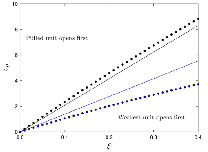
Figure 2.8: Phase diagram for the unfolding pathway in the pulling velocity-asymmetry plane for the more complex situation with two critical velocities. Now, we have three well-defined regions, separated by two curves, respectively, critical velocities $v_{c}^{(1)}$ (blue) and $v_{c}^{(2)}$ (black) vs. asymmetry $\xi$. Note that our theoretical approach is able to reproduce the existence of the three different pulling regimes. Nevertheless, the discrepancies between theoretical and numerical values for the critical velocities are larger than those in figures 2.6 and 2.7.

We check the more complex scenario described in the previous paragraph in figure 2.8. On the one hand, our theory correctly predicts the existence of the three pulling regimes described above. On the other hand, even for very small asymmetries, there appear some noticeable discrepancies between theory and simulation. The validity of the perturbative expansion for obtaining the critical velocities, expressed by condition (2.27), is strongly supported by the accurateness of the theoretical prediction for the simplest case with only one critical velocity, see figures 2.6 and 2.7. Then, we believe that this discrepancy stems from the intrinsically approximate character of the condition $a^{\prime\prime}_{i}=0$ for determining the stability threshold for finite pulling velocity $v_{p}\neq 0$. Thus, improving the present theory should involve the derivation of a more accurate condition for the stability threshold in this case. This refinement to our theoretical framework, which probably makes a multiple scale analysis necessary for lengths close to the condition $a^{\prime\prime}=0$, is an open question that deserves further investigation.

2.5 Moving closer to the experiment

Now, we try to get closer to the experiment. We do so by introducing some variants of the basic model we have analyzed in the previous sections. The main idea is to sophisticate the model to make it more realistic, and test the robustness of our theoretical results.

In a real AFM experiment, the stiffness is finite and, as a result, the control over the length is not perfect. Furthermore, the position that is externally controlled is, usually, that of the platform and the main elastic force stems from the bending of the tip of the cantilever, as depicted in figure 1.3.

Some authors [120] have used other elastic reactions that reflect the attachment by means of flexible linkers among the platform and the pulled end, and between consecutive modules. Here, we will consider a perfect absorption, in order to keep the model as simple as possible.

Also, the procedure followed in the previous sections for making the free energy of one unit different from the rest may be considered a little bit artificial. Therefore, we also introduce here a more physical way of perturbing the free energies. Specifically, we do so by changing the contour length of the corresponding module.

This section is structured as follows. We study the effect on the unfolding pathway of the finite value of the stiffness and the location of the spring, in sections 2.5.1 and 2.5.2, respectively. Finally, section 2.5.3 is devoted to analyze the perturbation of the free energy of one unit brought to bear by the change of its contour length.

2.5.1 Finite stiffness

Here, we still consider the basic model depicted in figure 2.1, with the spring located at the pulled end. Notwithstanding, we assume unperfect length control, that is, the stiffness $k_{c}$ of the spring is finite. Still, we consider the macroscopic equations (zero noise), which are

$$\gamma\dot{x}_{1}= -a^{\prime}_{1}(x_{1})+a^{\prime}_{2}(x_{2}),$$ (2.48a)

$$\gamma\dot{x}_{i}= -2a^{\prime}_{i}(x_{i})+a^{\prime}_{i+1}(x_{i+1})+a^{\prime}_{i-1}(x_{i-1}),\quad 1<i<N,$$ (2.48b)

$$\gamma\dot{x}_{N}= -2a^{\prime}_{N}(x_{N})+a^{\prime}_{N-1}(x_{N-1})+k_{c}\left(L-\sum_{k=1}^{N}x_{k}\right).$$ (2.48c)

This system differs from that in (2.7) because, in the last equation, the Lagrange multiplier $F$ is substituted by the harmonic force $k_{c}(L-\sum_{k}x_{k})$. As in the previous case, this system is analytically solvable by means of a perturbative expansion in $v_{p}$ and $\xi$. The approximate solution for the extension $x_{i}$ is

$$x_{i}=\ell+ \frac{\xi Nk_{c}\overline{\delta f}(\ell)-v_{p}\gamma k_{c}\dfrac{[3U^{\prime\prime}(\ell)+k_{c}(N-1)]N(N+1)}{6[Nk_{c}+U^{\prime\prime}(\ell)]}}{U^{\prime\prime}(\ell)[Nk_{c}+a^{\prime\prime}(\ell)]}$$

$$+ \frac{v_{p}\gamma k_{c}i(i-1)-2\xi[Nk_{c}+a^{\prime\prime}(\ell)]\delta f_{i}(\ell)}{2a^{\prime\prime}(\ell)[Nk_{c}+a^{\prime\prime}(\ell)]}.$$ (2.49)

Here $\ell\neq L/N$, it stems from the relation

$$a^{\prime}(\ell)=k_{c}(L-N\ell).$$ (2.50)

We can see easily how we reobtain (2.26) taking the limit $k_{c}\to\infty$ in (2.49), as it should be. Although the solution is slightly different, it still breaks down when $a^{\prime\prime}(\ell)$ vanishes, that is, when $\ell\to\ell_{b}$. Therefore, to the lowest order, again we have to seek a solution of (2.27), with the extensions given by (2.49), and substitute $\ell_{c}\simeq\ell_{b}$ therein. This leads to the same critical velocities found for the infinite stiffness limit.

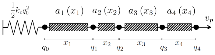
Figure 2.9: Sketch of the model for a protein with four units. It is identical to figure 2.1, except for the position of the length control device, which is now located at the fixed end.

2.5.2 Location of the elastic reaction

As depicted in figure 1.3, in an AFM experiment the distance between the moving platform and the fixed cantilever is the controlled quantity. Then, the model sketched in figure 2.9 is closer to the experimental setup: the left end corresponds to the fixed cantilever, with $q_{0}$ standing for $\Delta X$, and the right end represents the moving platform. Thus, the free energy of this setup is given by

$$A(q_{0},\ldots,q_{N})=\sum_{i=1}^{N}a_{i}(q_{i}-q_{i-1})+\frac{1}{2}k_{c}q_{0}^{2}\,.$$ (2.51)

From the free energy (2.51), we derive the Langevin equations by making use of (2.2). The macroscopic equations (zero noise) read

$$\gamma\dot{x}_{1}= -2a^{\prime}_{1}(x_{1})+a^{\prime}_{2}(x_{2})+k_{c}\left(L-\sum_{k=1}^{N}x_{k}\right),$$ (2.52a)

$$\gamma\dot{x}_{i}= -2a^{\prime}_{i}(x_{i})+a^{\prime}_{i+1}(x_{i+1})+a^{\prime}_{i-1}(x_{i-1}),\quad 1<i<N,$$ (2.52b)

$$\gamma\dot{x}_{N}= -a^{\prime}_{N}(x_{N})+a^{\prime}_{N-1}(x_{N-1})+\gamma v_{p}.$$ (2.52c)

In the infinite stiffness limit, $k_{c}\to\infty$, the harmonic contribution in (2.52a) tends to a new Lagrange multiplier $F$ such that $\sum_{i}x_{i}=L$. By summing up all the equations, it is obtained that $F=a_{1}^{\prime}(x_{1})$ and the resulting system is exactly equal to that in (2.7). This is logical: if the spring is totally stiff and then the control over the length is perfect, the two models are identical. It is worth emphasizing that the two variants of the model, with the spring at either the fixed or moving end, have the same number of degrees of freedom. In the original model, the left end is fixed, $q_{0}=0$ and our degrees of freedom are $q_{i}$, $i=1,\ldots,N$, whereas in figure 2.9 we have the dynamical constraint $q_{N}=L$ and the degrees of freedom are $q_{i}$, $i=0,\ldots,N-1$. In the limit as $k_{c}\to\infty$, we have the constraints $q_{0}=0$ and $q_{N}=L$ in both models, making it obvious that they are identical.

The system (2.52) with finite stiffness can be solved in an analogous way, by means of a perturbative expansion in the asymmetry $\xi$ and the pulling velocity $v_{p}$. The result is

$$x_{i}=\ell+ \frac{\xi Nk_{c}\overline{\delta f}(\ell)-v_{p}\gamma k_{c}\dfrac{[3a^{\prime\prime}(\ell)+k_{c}(N-1)]N(N+1)}{6[Nk_{c}+a^{\prime\prime}(\ell)]}}{a^{\prime\prime}(\ell)[Nk_{c}+a^{\prime\prime}(\ell)]}$$

$$+ \frac{v_{p}\gamma k_{c}i\left(i-1+\dfrac{2a^{\prime\prime}(\ell)}{k_{c}}\right)-2\xi[Nk_{c}+a^{\prime\prime}(\ell)]\delta f_{i}(\ell)}{2a^{\prime\prime}(\ell)[Nk_{c}+a^{\prime\prime}(\ell)]},$$ (2.53)

where $\ell$ is again given by (2.50). Of course, we can reobtain (2.26) by taking the infinite stiffness limit in (2.53). Although the final solution for the extension is different from the previous one, when we look for the critical velocities and make the approximation $\ell_{c}\simeq\ell_{b}$ we get the same analytical results for them.

The main conclusion of the last two sections, 2.5.1 and 2.5.2, is that the existence of a set of critical velocities, setting apart regions where the first unit to unfold is different, is robust. In particular, it is not an artificial effect of either the limit $k_{c}\to\infty$ or the location of the spring. Indeed, at the lowest order, all the variants of the model give the same critical velocities. This robustness is an appealing feature of our theory, which makes it reasonable to seek the predicted phenomenology in real experiments.

2.5.3 Units with different contour lengths

In the experiments, the observation of the unfolding pathway is not trivial at all. The typical outcome of AFM experiments is a force-extension curve in which the identification of the unfolding events is, in principle, not possible when the modules are identical. Thus, in order to test our theory, molecular engineering techniques that manipulate proteins adding some extra structures, such as coiled-coil [129] or Glycine [130] probes, come in handy. For instance, a polyprotein in which all the modules except one have the same contour length may be constructed in this way. A reasonable model for this situation is a chain with modules described by Berkovich’s potentials (2.41) with the same parameters for all the modules, with the exception of the contour length of one of them. According to our discussion in section 2.3, this configuration is one of the simplest in which a critical velocity, as given by (2.36), emerges. In addition, this peculiar behavior may be observed in real experiments, because the unfolding of the unit that is different can be easily identified in the force-extension curve, see next section.

Then, we consider that the free energy of the different unit is perturbed in the more physical way described above. Accordingly, we change the module’s free energy by considering that the contour length of the module is slightly increased, from $L_{c}$ to $L_{c}+\Delta$. Consistently, we use $a(x)=a_{B}(x;L_{c})$ to represent the free energy of each of the identical modules, and $a_{1}(x)=a_{B}(x;L_{c}+\Delta)$ for that of the first one. We have explicitly introduced in the notation that the only difference between the first unit and the rest is the slightly different contour length. Thus, we can linearize $a_{1}(x)$ around $a(x)$, using the natural, dimensionless, asymmetry parameter $\xi=\Delta/L_{c}\ll 1$. Therefore,

$$a_{1}^{\prime}(x)\simeq a_{B}^{\prime}(x;L_{c})+\xi\delta f_{1}(x;L_{c}),$$ (2.54)

where

$$\delta f_{1}(x;L_{c})\equiv L_{c}\frac{\partial a_{B}^{\prime}(x;L_{c})}{\partial L_{c}}=-\frac{k_{B}T}{2P}\left[\frac{\frac{x}{L_{c}}}{\left(1-\frac{x}{L_{c}}\right)^{3}}+\frac{2x}{L_{c}}\right].$$ (2.55)

The linearization in (2.54) is useful for the direct application of our theory to some engineered systems, see next section. We would like to emphasize that $\delta f_{1}(x;L_{c})<0$, since the function between brackets is always positive for $0<x<L_{c}$. That means that, for two units described by Berkovich’s free energy (2.41) with the same values for all parameters except the contour length, the weakest unit is the longest one.

2.6 Experimental prospect

Let us consider an example of a possible real experiment for a polyprotein with $N=10$ modules. We characterize the modules by Berkovich’s potentials with the parameters introduced in (2.46), with $k_{B}T=4.2\text{ pN}\,\text{ nm}$ and friction coefficient $\gamma=0.0028$pN nm^-1s [126]. We call this system M₁₀: since all the modules are equal in M₁₀, it is not a very interesting system from the point of view of our theory. Nevertheless, now we can resort to the ideas we have just put forward. Thus, we consider a mutant species M${}^{\prime}_{10}$ that is identical to M₁₀, except for the module located in the first position (the fixed end), which has an insertion adding $\Delta$ to its contour length. Our theory gives an estimate for the critical velocity $v_{c}$ by inserting (2.55) into (2.36) with $\alpha_{1}=1$.

In figure 2.10, we compare the theoretical estimate for the critical velocity with the actual critical velocity obtained by integration of the dynamical system (2.52). Specifically, we have considered a system with spring constant $k_{c}=100$pN/nm. The numerical strategy to determine $v_{c}$ has been quite similar to that in section 2.4.2: starting from a completely folded state we let the system evolve obeying (2.52), with a “high” value of $v_{p}$—well above the critical velocity—, up to the first unfolding. We tune $v_{p}$ down until it is observed that the first module that unfolds is the weakest one: this marks the actual critical velocity. There are two theoretical lines: the solid line stems from the rigorous application of (2.36), with $\delta f_{1}$ given by (2.55), and $v_{c}$ is a linear function of $\xi$, whereas the dashed line corresponds to the substitution in (2.36) of $\xi\delta f_{1}(x)$ by $a_{B}^{\prime}(x;L_{c}+\Delta)-a_{B}^{\prime}(x;L_{c})$, without linearizing in the asymmetry $\xi$. Note the good agreement between theory and numerics, especially in the “complete” theory where, for the range of plotted values, the relative error never exceeds 5$\%$. Interestingly, most of the computed values of the critical velocity lie in the range of typical AFM pulling speeds, from $10$ nm/s to $10^{4}$ nm/s [13].

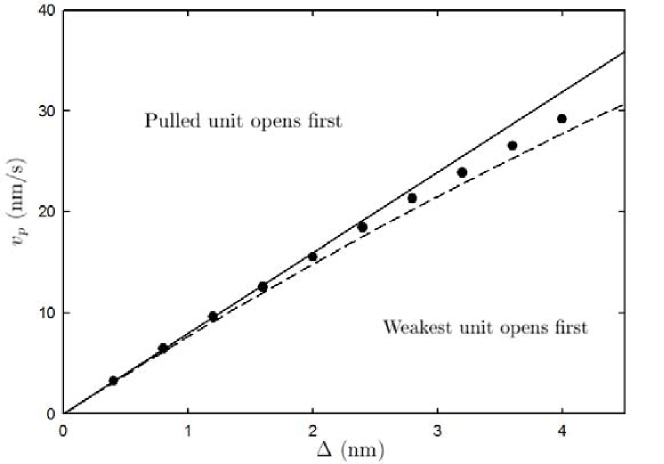
Figure 2.10: Critical velocity in the M${}^{\prime}_{10}$ system. The parameter $\Delta$ is the first module’s additional contour length. Numerical values (circles) are compared with two theoretical results: “complete” (dashed line) and linear (solid line).

Below the critical velocity $v_{c}$, it is always the weakest unit that unfolds first. Above $v_{c}$, the unit that unfolds first is the pulled one. For the sake of concreteness, from now we consider a specific molecule M${}^{\prime}_{10}$ fixing $\Delta=2$ nm. Inserting the linear estimation (2.55) into (2.36), we get a critical velocity $v_{c}\simeq 16$ nm/s, which is in the range of typical pulling speeds in AFM experiments.

In figure 2.11, we plot the extension of each unit vs the total extension $q_{N}-q_{0}$ in our notation ($L$ in figure 1.3). We have numerically integrated (2.52) for two values of $v_{p}$: one below and one above $v_{c}$, namely $v_{p}=10$ nm/s and $v_{p}=22$ nm/s. The red trace stands for the weakest unit extension whereas the blue one corresponds to the pulled module. We can see that, for $v_{p}=10\text{ nm/s}<v_{c}$, the first unit that unfolds is the weakest one, whereas for $v_{p}=22\text{ nm/s}>v_{c}$ that is no longer the case. Specifically, the first unit that unfolds is the pulled one, and the weakest unfolds in the fourth place.

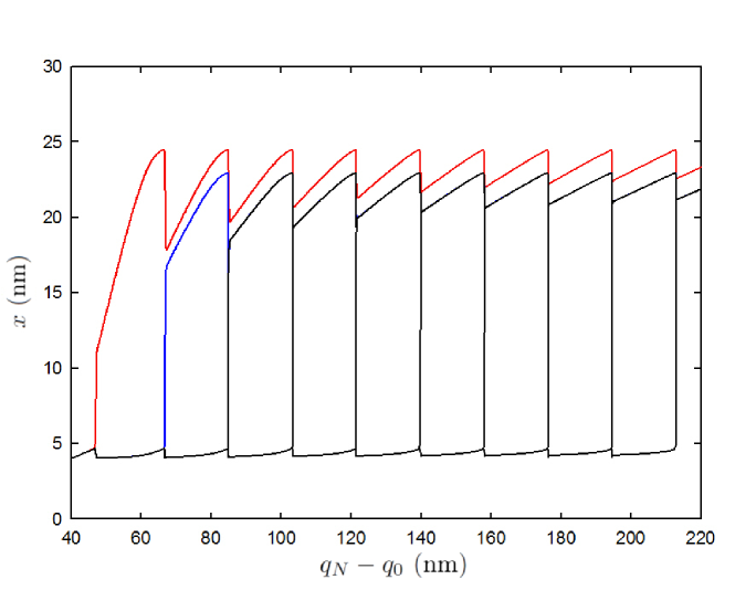
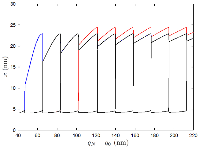
Figure 2.11: Evolution of the units’ extensions as a function of the system length $q_{N}-q_{0}$. The potential parameters are given in (2.46), and the pulling speeds are $v_{p}=10$ nm/s $<v_{c}$ (top) and $v_{p}=22$ nm/s $>v_{c}$ (bottom). The stiffness is $k_{c}=100$ pN/nm, which lies in the range of typical AFM values. The red line corresponds to the weakest unit and the blue line to the pulled one.

The plots in figure 2.11 are the most useful in order to detect the unfolding pathway of the polyprotein. Unfortunately, they are not accessible in real experiments, for which the typical output is the force-extension curve, as already stated above. As a consequence, we have also plotted the force-extension curve in order to bring to light the expected outcome of a real experiment. In figure 2.12, we show the force-extension curve for the two considered velocities in the same graph (solid line for the lower speed and dashed line for the higher one).

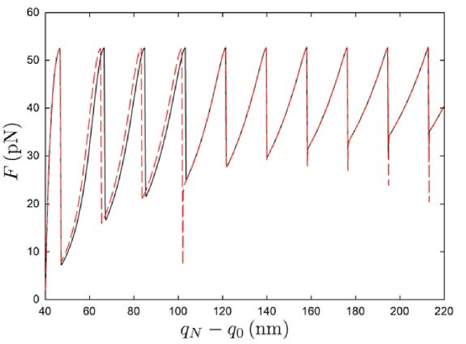
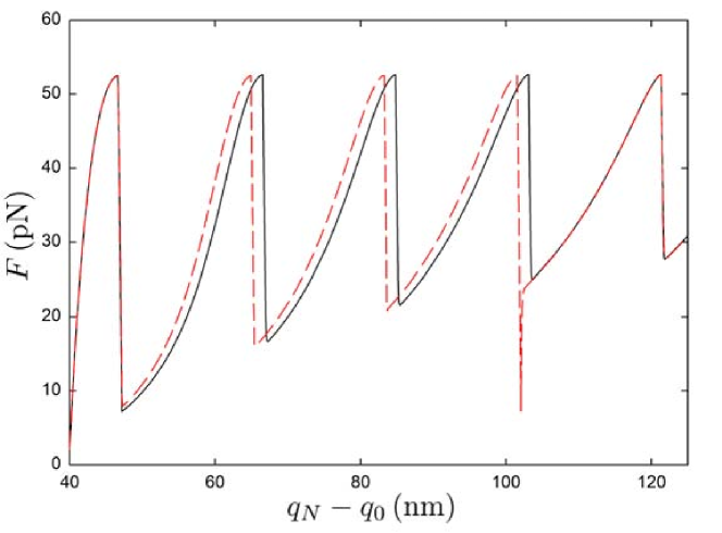
Figure 2.12: (Top) Force-extension curve corresponding to the pulling experiment in figure 2.11. Specifically, we consider two pulling velocities $v_{p}=10$ nm/s (subcritical, solid) and $v_{p}=22$ nm/s (supercritical, dashed). (Bottom) Zoom of the region of interest, which clearly shows the shift between the peaks stemming from the increased contour length of the mutant unit.

The force-extension curves in figure 2.12 are superimposed until the first force rip, which corresponds to the first unfolding event: that of the mutant module for the slower velocity and that of the pulled unit for the faster one. As the mutant unit has a longer contour length than the rest, a shift between the curves in the next three spikes is found. This shift stems from the effective contour length of the polyprotein having an extra contribution of $2$ nm. Reasonably, for the higher velocity, this shift disappears when the mutant module unfolds. Thenceforth, the force-extension curves are once again superimposed. This plot clearly shows how the emergence of a critical velocity could be sought in a real experiment.

Chapter 3 Testing the model with molecular dynamics

The theoretical approach developed in the previous chapter is clearly a drastic simplification of reality. In fact, the final result of our theory is deterministic, in the sense that the unfolding pathway is a definite one, the randomness coming from thermal fluctuations being effectively “suppressed” by the fast enough pulling velocity. In reality, as also discussed in chapter 2, the unfolding pathway does have some degree of stochasticity, stemming from the interactions between the molecule under study and the fluid where it is immersed, which are encoded in the Gaussian white noises of our Langevin description.

Testing the theory is a mandatory step of scientific method. The task of performing real pulling experiments with a modular protein that matches all the requirements of our theoretical framework is not simple at all. Therefore, in this chapter, we focus on steered molecular dynamic (SMD) of engineered systems. Since the first investigations made by Grubmüller [131] and Schulten [132], these computational techniques have shown to be of crucial relevance in the current development of biophysics [133, 134, 135]. To test our theoretical predictions, we consider a particularly simple structure composed of coiled coils. This kind of structures is common in nature, which makes it extremely useful as a model system [136, 137, 138].

The organization of the chapter is as follows. Section 3.1 is devoted to stress the relevance of the hypotheses assumed in the theory developed in the previous chapter. Also, we discuss its applicability to specific molecules in specific ranges of velocities. Therein, we introduce the construct we work with throughout this chapter, which comprises two consecutive coiled-coil structures. The simulation procedure along with the method employed for the data analysis are presented in section 3.2. Specifically, we explain how we acquire the initial configurations from which the construct is pulled. In section 3.3, the results of our simulations are put forward, and they are compared with our theoretical prediction. A key point in our numerical analysis is our assumption about the independence of the initial conditions chosen for the pulling stage. Then, in section 3.4, we prove this data acquisition to be actually uncorrelated, within the accuracy of our statistics.

3.1 The candidate protein

We expect our theoretical approach to hold for some molecules within a specific range of pulling velocities. One of the obvious requirements our protein candidate must meet is a negligible interaction between repeats, since we have assumed no nearest-neighbor interaction terms in the global free energy. Regarding the range of velocities, if pulling is very slow and quasistatic, the first unfolding event occurs at the length value for which the free energy minima over the branch with all the units folded and over the branch with only one unit unfolded are equally deep [39]. Therein, the jump between branches occurs by thermal activation over the free energy barrier separating them. As a consequence, the completely folded branch is only partially swept, as marked by the dashed vertical (red) lines in figure 3.1. In contrast, there is a range of fast pulling velocities that do not give the system enough time to be thermally activated over the barrier, but are slow enough to allow it to sweep completely the part of the branches that corresponds to metastable equilibrium states. In this case, the jump between branches comes about at the limit of metastability, only when the folded minimum disappears [41], as depicted in the top panel of figure 3.1. This is marked by the solid vertical (blue) lines in the bottom panel of figure 3.1. This range of adiabatic velocities we are interested in, as defined in chapter 2, are also said to lead to the “maximum hysteresis path” [42], regime briefly introduced at the end of section 1.1.2.

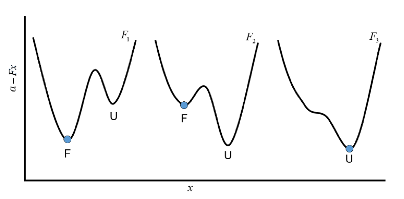
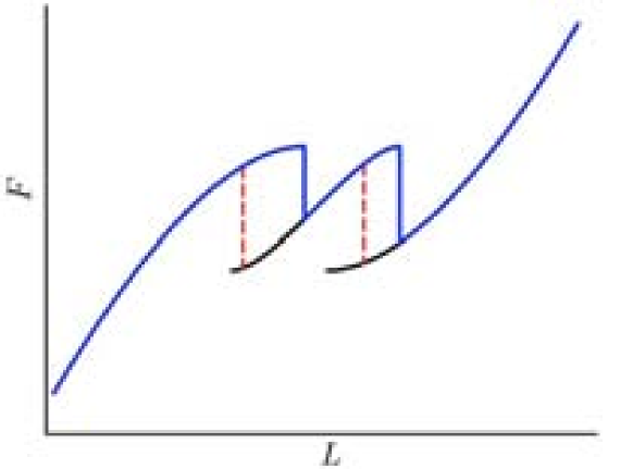
Figure 3.1: (Top) Schematic free energy landscape of a single repeat for three different forces $F_{1}<F_{2}<F_{3}$. The system starts in the folded (F) state, which is the absolute minimum for $F_{1}$. If thermal noise is negligible, the repeat remains in the folded state for $F_{2}$ even when the unfolded state is more stable. For $F_{3}$, the F state disappears, and the repeat finally unfolds. (Bottom) Qualitative picture of the stability branches in a modular system with two units. The blue line shows the unfolding pathway followed in the limit of the so-called “maximum hysteresis path”, when the pulling speed is high enough to make the system sweep the whole branches, including their metastable parts. In this limit, the jumps between consecutive branches take place by the mechanism shown in the top panel because the system does not have enough time to jump over the barrier separating the folded and unfolded states. In other words, the “fast enough” pulling speed effectively suppresses thermal fluctuations. Conversely, in the quasistatic limit the transition from folded to unfolded takes place at the lengths (dashed red lines) at which the branch with one more unfolded unit becomes more stable, that is, when its free energy becomes smaller. For the quasistatic case, the system has always time to find its way through the barrier.

We have designed a simple homopolyprotein, which we employ below to test whether it fits our theoretical description. We have extracted the structure of an antiparallel coiled-coil motif (CC) from the archeal box C/D sRNP core protein (Protein Data Bank entry 1NT2), which comprises 67 residues and whose N-terminus and C-terminus are, respectively, arginine (ARG) and isoleucine (ILE) [139]. This structure has been proven to be useful as a mechanical folding probe [129]. We use this CC as the building blocks of the molecule: our system is simply a concatenation of two CC motives connected by a linker, which is composed of two consecutive pairs of alternated residues of glycine and serine. We expect this linker not to introduce any significant interaction between the two domains. The initial conformation of the constructed model structure and orientation of the two CC repeats is shown in figure 3.2. The end- to-end vector points from the N-terminus to the C-terminus, aligned with the $x$-axis, whereas both axial directions of the two CC structures are located as parallel as possible to the $z$-axis.

According to the theoretical framework we have developed along this work, since we have two identical units, we expect that if we pull from one end of the designed molecule, the first repeat to unfold will be precisely the closest to the moving end. We perform SMD simulations to analyze the degree of agreement of the obtained numerical results with the theory.

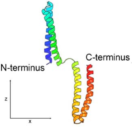
Figure 3.2: Initial conformation of the homopolyprotein comprising two CCs in the SMD simulations. The pulling direction is aligned with the $x$-axis, whereas the axial directions of the CCs are aligned with the $z$-axis.

3.2 All-atom molecular dynamics simulation

Our molecular dynamics simulations start from the initial conformation shown in figure 3.2. First, we add hydrogen atoms using VMD Automatic PSF Builder [140]. Then, we create a water box of size $300\textrm{\AA}\times 70\textrm{\AA}\times 120\textrm{\AA}$, in the $x$-, $y$-, and $z$-axes, respectively, which is long enough in the direction of pulling (the $x$-axis) to contain the unfolded protein. Also, NaCl is introduced in the system replacing water molecules until the concentration reaches $150\,$mM/L and the charge is neutralized. Finally, simulations are performed using NAMD2 2.10 [141], with two different stages: (i) the “equilibration stage” at $310\,$K and (ii) the “pulling stage” with velocity $v_{0}=1.4\cdot 10^{-2}\,$nm/ps and stiffness $4860\,$pN/nm. We have also considered faster pulling velocities, namely $2v_{0}$ and $5v_{0}$, as detailed below. The molecule’s behavior for these faster pulling velocities has been investigated in order to elucidate whether or not the unfolding pathway becomes more deterministic as the pulling speed is increased.

These typical pulling speeds in steered molecular dynamics simulations are higher by several orders of magnitude than the experimental ones. However, they are necessary to investigate this kind of system with the available computer power. In addition, this high velocity range is especially relevant for our present purposes, since we are interested in exploring the maximum hysteresis path limit. Note that the considered value for the stiffness of the elastic reaction is also two orders of magnitude higher than the typical ones in AFM experiments, and thus closer to the perfect length control situation assumed in the theory developed in chapter 2.

3.2.1 Pulling trajectories

A notable number of pulling trajectories $N_{T}$ are needed in order to obtain a meaningful statistical analysis of the unfolding pathway. The final configuration of the molecule in the equilibration stage is taken as the initial condition for the pulling stage. In order to generate different initial conditions for pulling, we have considered one “long” trajectory in the equilibration stage and collected the molecule configurations at several different times $t_{k}$, with $t_{k+1}-t_{k}>0.1\,$ns, as the initial conditions for the different pulling trajectories $k=1,\ldots,N_{T}$. We have checked the “independence” of the trajectories obtained from these initial conditions, in the sense that the unfolding pathway from two consecutive initial conditions, corresponding to $k$ and $k+1$, are not correlated. Details are given in section 3.4.

The duration of the pulling stage $\Delta t_{p}$ is chosen to allow the molecule to unravel. The size of a single CC motif in its axial direction is around 5 nm, specifically 4.82 nm between the two C$\alpha$s most separated in the axial direction. Therefore, a motif can be considered as completely unfolded when its end-to-end distance, measured between their C$\alpha$s in the terminal residues ARG and ILE, exceeds 10 nm. For the “base” velocity $v_{0}=1.4\cdot 10^{-2}\,$nm/ps, we have chosen $\Delta t_{p}=1.6\,$ns, so that the total length increment is $v_{0}\Delta t_{p}=22.4\,$nm. For the faster pulling velocities, $2v_{0}$ and $5v_{0}$, we have decreased $\Delta t_{p}$ accordingly.

In SMD simulations, the length of each repeat can be measured as a function of time and thus we may introduce the basic (and the simplest) classification of trajectories by labeling them as “good” (G) if the CC motif closest to the pulled end unfolds sooner than the furthest, and “bad” (B) otherwise. Clearly, it is G-trajectories that agree with the prediction of the theory developed in chapter 2, when particularized for identical units. The above basic classification of SMD trajectories as G or B can be refined, so as to have a more accurate description of the unfolding pathway, as done below in section 3.2.2. In our theoretical framework, the unfolding is sequential: when the first unit unfolds, the second one has not reached its limit of stability and thus remains in the folded state. However, in the simulations, this perfectly sequential unfolding is not always found: when the first unit unfolds, the second one can be partially unfolded, see also section 3.3.

3.2.2 Unfolding criterion

Following the discussion in the previous paragraph and for the sake of accuracy, we define a criterion for distinguishing between different subtypes of trajectories. Therefore, we incorporate a quantitative measurement of the degree of unfolding for each repeat; first in a geometric way, and second taking into account the fraction of native contacts [142]. As already said above, the size of the CC motif in its axial direction is approximately $5\,$nm and thus we consider a motif to be completely unfolded when its end-to-end distance is greater than $10\,$nm. Also, we define when a motif is partially unfolded in our simulations by introducing an “unfolding threshold”, that is, a length below which we consider the unit to be still folded. Specifically, we take this unfolding threshold to be $7\,$nm, which corresponds to an opening angle of $90^{\circ}$ in a rigid rods picture, as depicted in figure 3.3.

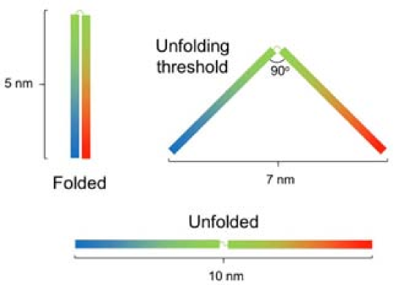
Figure 3.3: Simple unfolding criterion for the CC under study. This criterion is based on a rigid-rod picture. Depending on the value of its end-to-end distance, we consider the molecule as (i) folded if it is shorter than 7 nm, (ii) partially unfolded when it is between 7 and 10 nm, and (iii) completely unfolded if it is longer than 10 nm.

The above “geometric” choice for the unfolding threshold has some degree of arbitrariness, especially in relation to the length (or angle between rigid-rods) chosen for the unfolding threshold. In order to give a physical basis for this choice, we look into the fraction of native contacts [142] as a function of the total length for a single CC motif in figure 3.4. For this purpose, we have performed a SMD simulation in which a single CC motif, which is initially folded, is pulled at a speed of $3.75\cdot 10^{-3}\,$nm/ps from either its C-terminus (blue) or its N-terminus (red). It can be observed how the number of native contacts decreases along the trajectory, with a well-defined plateau arising between (approximately) 7 and 10 nm. Clearly, the borders of this plateau demarcate the region where the main bonds that keep the double-stranded CC folded are broken. Therefore, the above-defined geometric thresholds for considering the molecule folded/partially unfolded/completely unfolded agree with the corresponding limits in the fraction-of-native-contacts picture.

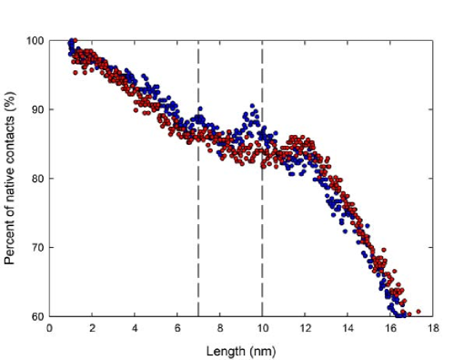
Figure 3.4: Percentage of native contacts as a function of the total length. Both the data from C-pulling (blue) and N-pulling (red), at a speed $3.75\cdot 10^{-3}\,$nm/ps, are plotted. The borders of the plateau agree quite well with the thresholds up to (from where) we consider the molecule to be folded (unfolded) in the geometrical picture, marked with vertical dashed lines.

Consistently with the above-described criteria, let us index the different subtypes of trajectories by (I, II, III, IV), attending to their degree of agreement with the theoretical prediction. G-trajectories are split into I and II subtypes: when the pulled motif is the first that unfolds, the other unit can be either still folded (type I) or partially unfolded (type II). Similarly, B-trajectories are divided into III and IV subtypes: when the non-pulled motif unfolds first, the pulled unit can be either partially unfolded (type III) or still folded (type IV). The explicit distinction between the different cases, for a simulation in which the molecules is pulled from its C-terminus, is shown in table 3.1. Obviously, if the molecule is pulled from its N-terminus, the same classification of trajectories applies but with the role of the repeats C and N reversed.

Table 3.1: Definition of the different trajectory types in a SMD C-pulling simulation. Types I and IV are the closest trajectories to a deterministic pathway, agreeing and disagreeing, respectively, with the prediction of our model.

Type	Subtype	First repeat that unfolds	State of the other repeat
Good (G)	I	C-terminus	folded
Good (G)	II	C-terminus	partially unfolded
Bad (B)	III	N-terminus	partially unfolded
Bad (B)	IV	N-terminus	folded

3.3 Pulling the CC construct

In this section, we present the SMD results corresponding to the pulling of the CC construction described above. We consider the two possible experiments, pulling from the C-terminus (C-pulling) and from the N-terminus (N-pulling), separately.

3.3.1 C-pulling

First, we pull the molecule from its C-terminus at the base velocity $v_{0}=1.4\cdot 10^{-2}\,$nm/ps. We plot the evolution of the distance between the end terminals of each repeat in this C-pulling experiment in figure 3.5. The red line stands for the pulled repeat (C-terminus) whereas we plot in blue the length of the other repeat (N-terminus). It can be seen how the pulled repeat clearly unfolds first in type I. Although from different categories, types II, III and IV seem to share a common feature. In the initial part of the trajectory, it is the pulled repeat the fastest to lengthen but its unfolding comes to a standstill before being completed, and the second repeat takes advantage of this impasse to increase its extension.

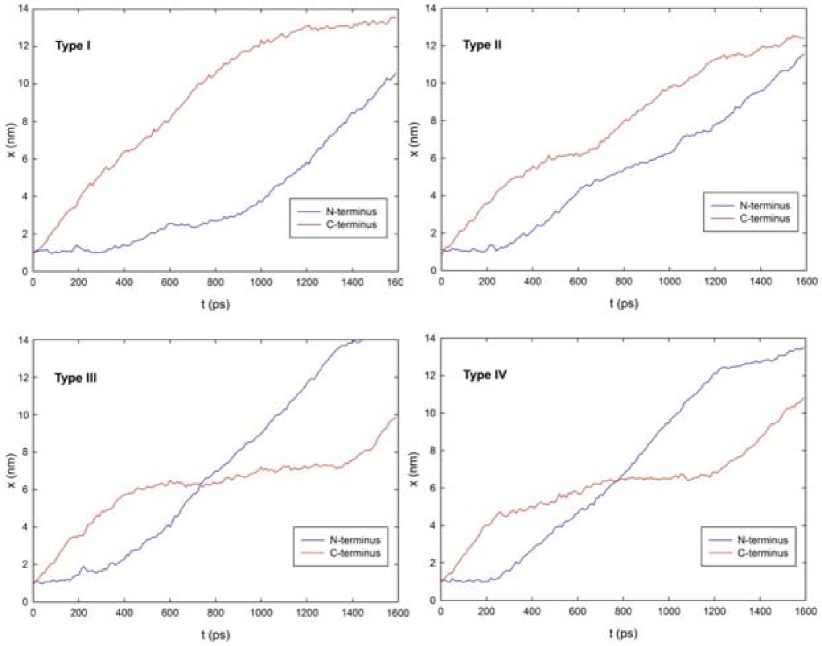
Figure 3.5: Representative plots of the different types of trajectories for SMD C-pulling simulations. Each panel corresponds to a given type, as labeled. Both repeats’ extensions are plotted: N-repeat (blue) and C-repeat (red). Our model predicts that the pulled repeat (C-terminus) is the first that unfolds. Videos corresponding to each of the trajectory types can be found in the supporting information to [143].

Due to thermal fluctuations, we do not expect to obtain a perfect agreement with our theory, but a preponderance of the deterministic (type I) trajectories. As discussed before, a “fast” pulling velocity is necessary to be in the “maximum hysteresis path” limit, in which our theory is expected to hold. Therefore, in addition to the base velocity $v_{0}=1.4\cdot 10^{-2}\,$nm/ps, we have carried out simulations at velocity $2v_{0}$. Specifically, we have done 31 trajectories for each velocity and collected their statistical information in table 3.2, which is completely compatible with our theoretical expectation. There is already a preponderance of type I trajectories at the base velocity $v_{0}$, at which they represent almost half of the total number of trajectories, against a reduced fraction, only 16$\%$, of type IV trajectories. Moreover, the prevalence of type I trajectories increases with the pulling velocity, as expected in our theoretical framework: at velocity $2v_{0}$, more than two thirds of the SMD runs are of type I and there are no type IV trajectories.

We can get additional insight by calculating the frequencies of G (sum of I+II) and B (sum of III+IV) trajectories. This simplification of the types of events shows, even more clearly, the preponderance of the deterministic path as the velocity is increased: the frequency of G-trajectories shows a clear increase from 61$\%$ at velocity $v_{0}$ to 87$\%$ at velocity $2v_{0}$ (the frequency of B-trajectories decreases accordingly from 39$\%$ to 13$\%$). This is the reason why we have not considered even higher velocities for C-pulling.

The above results show that increasing the pulling speed effectively diminishes the relevance of thermal activation effects and makes the unfolding more “deterministic”, in the sense of increasing the prevalence of type I trajectories. It should also be stressed that detailed analysis of the rest of type trajectories highlights a branching from type I due to an impasse of the length of pulled repeat, as already stated at the beginning of this section. Wrapping things up, our theory seems to predict the unfolding mechanism displayed in the SMD of this CC homopolyprotein—at least, when it is pulled from the C-end.

Table 3.2: Statistical analysis of the output of 31 runs of SMD C-pulling simulations of the two CCs construct. At the base velocity $v_{0}$, there is already a significant preponderance of type I trajectories (45$\%$) as compared to type IV ones (16$\%$). Type I trajectories clearly prevail as the pulling velocity is increased to $2v_{0}$, at which its frequency is boosted up to 67$\%$. In addition, no type IV trajectories are found at this higher velocity. This behavior clearly agrees with our theoretical prediction.

Type	Occurrence at $v_{0}$ ($\%$)	Occurrence at $2v_{0}$ ($\%$)
I	45	68
II	16	19
III	23	13
IV	16	0
Good = I + II	61	87
Bad = III + IV	39	13

3.3.2 N-pulling

Of course, our one-dimensional theory is completely left-right symmetric, since the free energy only depends on the extensions. Therefore, if we perform the same kind of SMD simulations but pulling from the N-terminus, we expect similar results (within statistical errors for the limited number of trajectories). Thus, the unfolding should start, preponderantly, from the unit closer to the N-terminus. Nevertheless, we show below that the situation is more complex, which we understand as a signature of anisotropy in the considered molecule.

Table 3.3 presents the statistics of the different types of trajectories for SMD simulations in which we pull from the N-terminus. In terms of the same base velocity $v_{0}=1.4\cdot 10^{-2}\,$nm/ps, we have conducted numerical experiments at velocities $v_{0}$, $2v_{0}$ and $5v_{0}$. Specifically, the statistics have been obtained again from 31 runs for each pulling velocity. The situation is much more complex than for C-pulling, since for both $v_{0}$ and $2v_{0}$ there is no clear preponderance of the deterministic pathway. On the one hand, the fraction of G-trajectories increases from less than half to more than two thirds as the pulling velocity is increased from $v_{0}$ to $2v_{0}$, which seems to indicate that the pathway is becoming more deterministic. On the other hand, the frequency of type I trajectories decreases in favor of those of type II. This complex behavior makes it necessary to consider a higher velocity, so as to ascertain the tendency of the pathway as the velocity is increased. Specifically, we have incorporated simulations with pulling velocity $5v_{0}$. For this velocity, almost every trajectory (97$\%$) is type I, again in agreement with our theoretical framework.

Table 3.3: Statistical analysis of the output of 31 runs of SMD N-pulling simulations of the two CCs construct. In addition to the pulling velocities $v_{0}$ and $2v_{0}$, already analyzed for C-pulling, we have considered a faster velocity $5v_{0}$.

Type	Occurrence at $v_{0}$ ($\%$)	Occurrence at $2v_{0}$ ($\%$)	Occurrence at $5v_{0}$ ($\%$)
I	29	13	97
II	13	55	3
III	23	29	0
IV	35	3	0
Good = I + II	42	68	100
Bad = III + IV	58	32	0

Anisotropy of biological systems has been extensively studied [144]. Indeed, in the work of Gao et al. [145], a coiled-coil system very similar to ours presents different unfolding kinetics depending on the direction of the pulling: N- or C-pulling. Therein, the observed N-pulling transition rates between folded and unfolded states were much higher than the C-pulling rates. This property is compatible with our observations: if transition rates are higher in N-pulling, thermally activated jumps from the folded to the unfolded state could be relevant for the slower pulling velocities, although they were not for C-pulling. In this situation, we expect the range of velocities in which the “deterministic” or “maximum hysteresis” prevails to depend on the end from which the molecule is pulled. Specifically, we expect it to be higher for N-pulling, in agreement with our observations. Anyhow, the deterministic pathway becomes largely preponderant when the pulling velocity is high enough, as confirmed by our N-pulling simulations with the fastest velocity $5v_{0}$.

3.4 Independence of the initial conformations for the pulling stage

A possible issue with our simulations stems from our choice of initial conformations for the pulling stage. Instead of equilibrating the system many times, we have chosen to run a long trajectory and pick different conformations along it as the initial conditions for the subsequent pulling. One may wonder, quite reasonably, whether these initial conditions for the pulling stage are really uncorrelated, as we implicitly are assuming, or not. In this section, we thoroughly discuss this issue.

Let us denote by $\Gamma_{k}$ the different $k=1,\ldots,N_{T}$ initial conformations used as initial conditions for the pulling stage. To check the independence of these initial conformations $\Gamma_{k}$ invoked in section 3.2.1, we have analyzed possible correlations between the observed pathways in consecutive runs $k$ and $k+1$. In particular, we have focused our attention on the four possible pairs of “good” (G) and “bad” (B) trajectories (GG, GB, BG, BB) for each case we have considered, i.e. for given pulled terminus and pulling speed.

The $k$-th pulling trajectory, for given pulled terminus and pulling speed, starts from conformation $\Gamma_{k}$. Let us introduce a stochastic variable $\zeta_{k}$ to identify the type to which the $k$-th trajectory belongs. Thus, $\zeta_{k}$ can have two values that are denoted by $\alpha$, that is, $\alpha$ is equal to either G or B. In consecutive runs, $k$ and $k+1$, the possible values of the pair ($\zeta_{k}$,$\zeta_{k+1}$) are denoted by $\alpha\beta$, that is, the four possibilities (GG, GB, BG, BB). We denote the number of pairs of consecutive trajectories with a certain outcome $\alpha\beta$ by $n_{\alpha\beta}$, which is

$$n_{\alpha\beta}=\sum_{k=1}^{N_{p}}\delta_{\zeta_{k},\alpha}\delta_{\zeta_{k+1},\beta}$$ (3.1)

where $N_{p}=N_{T}-1$ is the number of consecutive pairs and $\delta_{ij}$ is Kronecker delta.

The probability that any trajectory corresponds to a given type (G or B) can be formally written as

$$\left\langle\delta_{\zeta_{k},\alpha}\right\rangle=p_{\alpha}.$$ (3.2)

We are denoting the corresponding probabilities by $p_{\text{G}}$ and $p_{\text{B}}$, respectively, and $p_{G}+p_{B}=1$ because these events are mutually exclusive, $\delta_{\zeta_{k},\text{G}}=1-\delta_{\zeta_{k},\text{B}}$. Now, assuming the outcomes of consecutive trajectories to be independent, we can ask ourselves the following questions in an ensemble of simulations comprising $N_{T}$ trajectories (corresponding to a given pulled terminus and pulling speed).

1. What is the expected number of each pair type $\left\langle n_{\alpha\beta}\right\rangle$?

2. What are their corresponding standard deviations $\sigma_{\alpha\beta}$?

The mean value is directly obtained by taking into account (3.2), for all $k$, and the assumed statistical independence of the variables $\zeta_{k}$ and $\zeta_{k+1}$. Therefore, one gets straightforwardly that

$$\left\langle n_{\alpha\beta}\right\rangle=N_{p}p_{\alpha}p_{\beta}.$$ (3.3)

The derivation of the expression for the fluctuations is lengthier. We start by writing

$$n_{\alpha\beta}^{2}=\sum_{k=1}^{N_{p}}\sum_{l=1}^{N_{p}}\delta_{\zeta_{k},\alpha}\delta_{\zeta_{k+1},\beta}\delta_{\zeta_{l},\alpha}\delta_{\zeta_{l+1},\beta},$$ (3.4)

and we split the above expression into four contributions, corresponding to the cases (i) $l=k$, (ii)-(iii) $l=k\pm 1$, and (iv) all the other values of $l$. Thus, we can write

$$n_{\alpha\beta}^{2}= \sum_{k=1}^{N_{p}}\delta_{\zeta_{k},\alpha}\delta_{\zeta_{k+1},\beta}+\delta_{\alpha\beta}\sum_{k=1}^{N_{p}-1}\delta_{\zeta_{k},\alpha}\delta_{\zeta_{k+1},\alpha}\delta_{\zeta_{k+2,\beta}}$$

$$+\delta_{\alpha\beta}\sum_{k=2}^{N_{p}}\delta_{\zeta_{k-1},\alpha}\delta_{\zeta_{k},\alpha}\delta_{\zeta_{k+1,\beta}}+\sum_{k=1}^{N_{p}}\sum_{l\neq k,k\pm 1}^{N_{p}}\delta_{\zeta_{k},\alpha}\delta_{\zeta_{k+1},\beta}\delta_{\zeta_{l},\alpha}\delta_{\zeta_{l+1},\beta}.$$ (3.5)

Table 3.4: Frequencies (empirical and theoretical) and expected statistical errors for individual events and pairs of consecutive events. The values for the frequencies of G- and B-trajectory types are taken from tables 3.2 and 3.3.

Frequency	C-$v_{0}$	C-$2v_{0}$	N-$v_{0}$	N-$2v_{0}$	N-$5v_{0}$
G	0.61	0.87	0.42	0.68	1.00
B	0.39	0.13	0.58	0.32	0.00
GG	0.37	0.73	0.13	0.50	1.00
GG-th	0.38	0.76	0.18	0.46	1.00
GG-err	0.12	0.10	0.09	0.12	0.00
GB	0.23	0.13	0.27	0.17	0.00
GB-th	0.24	0.11	0.24	0.22	0.00
GB-err	0.05	0.05	0.05	0.05	0.00
BG	0.23	0.13	0.27	0.17	0.00
BG-th	0.24	0.11	0.24	0.22	0.00
BG-err	0.05	0.05	0.05	0.05	0.00
BB	0.17	0.00	0.33	0.17	0.00
BB-th	0.15	0.02	0.34	0.10	0.00
BB-err	0.08	0.02	0.11	0.07	0.00

Now we compute the average. We have four contributions on the rhs of the equation above: in the first sum, there are $N_{p}$ terms, each of them with average $p_{\alpha}p_{\beta}$; in both the second and third sums, there are $N_{p}-1$ terms, each of them with average $p_{\alpha}^{2}p_{\beta}$; and in the fourth sum we have the remaining $N_{p}^{2}-(3N_{p}-2)$ terms, each of them with average $p_{\alpha}^{2}p_{\beta}^{2}$. Once more, we have assumed the independence of the variables $\zeta_{k},\zeta_{l}$ for $l\neq k$. Thus, we get

$$\left\langle n_{\alpha\beta}^{2}\right\rangle=N_{p}p_{\alpha}p_{\beta}+2\delta_{\alpha\beta}\left(N_{p}-1\right)p_{\alpha}^{2}p_{\beta}+\left[N_{p}^{2}-\left(3N_{p}-2\right)\right]p_{\alpha}^{2}p_{\beta}^{2}.$$ (3.6)

The variance is thus given by

$$\sigma_{\alpha\beta}^{2}\equiv\left\langle n_{\alpha\beta}^{2}\right\rangle-\left\langle n_{\alpha\beta}\right\rangle^{2}=N_{p}p_{\alpha}p_{\beta}(1-3p_{\alpha}p_{\beta})+2p_{\alpha}^{2}p_{\beta}^{2}+2\delta_{\alpha\beta}\left(N_{p}-1\right)p_{\alpha}^{2}p_{\beta}.$$ (3.7)

For the sake of clarity, we list below the average values and the variances for the three pairs of outcomes leading to different values; note that $\left\langle n_{\text{GB}}\right\rangle=\left\langle n_{\text{BG}}\right\rangle$ and also $\sigma_{\text{GB}}=\sigma_{\text{BG}}$. Specifically,

$$\left\langle n_{\text{GG}}\right\rangle=N_{p}p_{\text{G}}^{2}, \sigma_{\text{GG}}^{2}=p_{\text{G}}^{2}\left(1-p_{\text{G}}\right)\left[N_{p}+p_{\text{G}}\left(3N_{p}-2\right)\right],$$ (3.8a)

$$\left\langle n_{\text{BB}}\right\rangle=N_{p}p_{\text{B}}^{2}, \sigma_{\text{BB}}^{2}=p_{\text{B}}^{2}\left(1-p_{\text{B}}\right)\left[N_{p}+p_{\text{B}}\left(3N_{p}-2\right)\right],$$ (3.8b)

$$\left\langle n_{\text{GB}}\right\rangle=\left\langle n_{\text{BG}}\right\rangle=N_{p}p_{\text{G}}p_{\text{B}}, \sigma^{2}_{\text{GB}}=\sigma^{2}_{\text{BG}}=N_{p}p_{\text{G}}p_{\text{B}}\left(1-3p_{\text{G}}p_{\text{B}}\right)+2p_{\text{G}}^{2}p_{\text{B}}^{2}.$$ (3.8c)

As expected, the variances would vanish if the process were purely deterministic and $p_{\text{G}}=1$ or, equivalently, $p_{\text{B}}=0$, since all the pairs would correspond to the GG case.

From an empirical point of view, we can identify $p_{\text{G}}$ and $p_{\text{B}}$ with the frequencies of G- and B-trajectories for the considered experiment (given pulled terminus/pulling speed). After doing that, we can count the actual number of pairs $n_{\alpha\beta}$ for each pair type in the ensemble of $N_{T}$ trajectories, and check if it lies within the theoretical expectation, for these empirical values of $p_{\alpha}$. What we show below is that for all our simulations we have that $\left|n_{\alpha\beta}-\left\langle n_{\alpha\beta}\right\rangle\right|\leq\sigma_{\alpha\beta}$, that is, the assumption of considering the initial conformations as independent is really good.

In order to give all the results in table 3.4, we list the empirical frequencies for each ensemble of trajectories, corresponding to a given pulled terminus and pulling speed. For example, C-$v_{0}$ means that the data in the corresponding column is for C-pulling at velocity $v_{0}$. For each column, the rows correspond to the frequencies for different events: (i) in the G and B rows, we give the empirical frequencies for good and bad trajectories, taken from tables 3.2 and 3.3; (ii) in the subsequent $\alpha\beta$ rows, the empirical frequencies for two consecutive trajectories of type $\alpha\beta$; (iii) in the $\alpha\beta$-th row, the corresponding theoretical prediction for that frequency, calculated as $\left\langle n_{\alpha\beta}\right\rangle/N_{p}$ from (3.8); (iv) in the $\alpha\beta$-err, we provide the theoretical prediction for the standard deviation of that frequency, calculated as $\sigma_{\alpha\beta}/N_{p}$ from (3.8). For the theoretical values of $\left\langle n_{\alpha\beta}\right\rangle/N_{p}$ and $\sigma_{\alpha\beta}/N_{p}$, we take $p_{\text{G}}$ and $p_{\text{B}}$ equal to the empirical frequencies of G- and B-trajectories, respectively, as already stated above.

Part II Understanding granular matter with simple lattice models

Chapter 4 Continuum limit, fluctuating hydrodynamics and finite size effects

Throughout this part of the thesis, we mainly investigate a lattice model for granular media inspired by two previous models on the lattice, specifically those in [146, 76]. The model differs from these two previous proposals in a few crucial aspects. First, in [146], the velocity field evolved under the enforcement of the so-called kinematic constraint, which is disregarded here. Second, in [76], only the energy field was considered, and therefore momentum conservation was absent.

Lattice models have been of paramount importance for understanding rigorously the conditions needed to have a hydrodynamic description, both at the average [68, 69] and fluctuating [67] levels. Recently, fluctuating hydrodynamics has been employed to derive the large deviation function in the context of energy-conserving [70, 71, 72, 73] and even in energy-dissipating [76, 75, 77, 78] models. Both in the conservative and nonconservative case, momentum conservation has not been taken into account. This shortcoming may be relevant, since it is known that momentum conservation is linked to the appearance of long-ranged correlations in out-of-equilibrium systems [147, 148]. More specifically, spatial long-range velocity correlations in the homogeneous cooling state can be partly explained by fluctuating hydrodynamics, but require a more refined treatment to be fully investigated.

This chapter is dedicated to introduce our model, from the basics to more involved issues. Our approach intends to contain the essential ingredients to investigate granular fluids, but reducing the complexity of the mathematical framework. In this way, we expect to get a transparent interpretation of the physical results. In particular, we aim to elucidate the “perturbative” nature of the continuum limit and calculate the corrections thereto [149]. Such corrections give interesting information about the structure—in space and time—of the correlated granular fluctuations and reveal new phenomena, which are peculiar of inelastic collisions.

The organization of this chapter is the following. In section 4.1, we briefly revise the main aspects of the model, focusing on its continuum, hydrodynamic-like, limit. A more detailed description of the model can be found in [79, 150, 151]. The evolution of the one-particle distribution function and some physically relevant stationary states are thoroughly analyzed, respectively, in sections 4.2 and 4.3. Section 4.4 is devoted to the study of the fluctuations of the system, including a discussion of their relation with some instabilities that appear in the model. Finally, we present an exact solution for the two-particle correlation function of the system in section 4.5, which is valid for arbitrary size and provides further insight into the instabilities.

4.1 Model and previous results

4.1.1 Evolution equations

Let us consider a 1d lattice with $N$ sites. First, we define the dynamics in discrete time. After the $p$-th step of the dynamics, the particle at the $l$-th site has a velocity $v_{l,p}\in$ $\mathbb{R}$, and the configuration for the system at time $p$ is denoted as $\bm{v}_{p}\equiv\{v_{1,p},...,v_{N,p}\}$. One individual trajectory of the stochastic process is built in the following way: the configuration of the system changes from time $p$ to time $p+1$ because a pair of nearest neighbors $\left(l,l+1\right)$ is chosen at random and collides inelastically, that is, $\bm{v}_{p+1}=\hat{b}_{l}\bm{v}_{p}$ where the operator $\hat{b}_{l}$ transforms the pre-collisional velocities $(v_{l,p},v_{l+1,p})$ into the post-collisional ones $(v_{l,p+1},v_{l+1,p+1})$ and leaves all other sites unaltered. The post-collisional velocities are given by

$$v_{l,p+1} = v_{l,p}-\frac{1+\alpha}{2}\Delta_{l,p},$$ (4.1a)

$$v_{l+1,p+1} = v_{l+1,p}+\frac{1+\alpha}{2}\Delta_{l,p},$$ (4.1b)

where $\Delta_{l,p}=v_{l,p}-v_{l+1,p}$ and the normal restitution coefficient is $\alpha\in(0,1]$. Note that, by its own definition, this stochastic process is Markovian. In the following, we use a notation such that the evolution operator $\hat{b}_{l}$ acts naturally on observables, for example, $\hat{b}_{l}v_{l,p}=v_{l,p+1}$. Momentum is always conserved,

$$(\hat{b}_{l}-1)(v_{l,p}+v_{l+1,p})=0,$$ (4.2)

whereas energy, if $\alpha\neq 1$, is not,

$$(\hat{b}_{l}-1)(v^{2}_{l,p}+v^{2}_{l+1,p})=(\alpha^{2}-1)\Delta_{l,p}^{2}/2<0.$$ (4.3)

The collision rule (4.1), which corresponds to the simplest one used in granular fluids [46], is valid for bulk sites. It must be complemented with suitable evolution equations for the sites next to the system boundaries, which depend on the physical situation at hand. See below for details.

The evolution equation for the velocities can be cast in the form

$$v_{l,p+1}-v_{l,p}=-j_{l,p}+j_{l-1,p},\quad j_{l,p}=\frac{1+\alpha}{2}\Delta_{l,p}\delta_{y_{p},l},$$ (4.4)

which is nothing but a discrete continuity equation. Therein, $j_{l,p}$ is the momentum current from site $l$ to site $l+1$ at time $p$, $\delta_{y_{p},l}$ is Kronecker’s delta, and $y_{p}$ is a homogeneously distributed random integer in $[1,L]$, where $L$ is the number of possible colliding pairs. For periodic boundary conditions, $L=N$, whereas for thermostatted boundaries $L=N+1$.

We have only kinetic energy, ${\cal K}_{p}=\sum_{l=1}^{N}e_{l,p}$ at time $p$, where $e_{l,p}=v_{l,p}^{2}$. By squaring (4.4), the evolution equation for the energy at site $l$ reads

$$e_{l,p+1}-e_{l,p}=-J_{l,p}+J_{l-1,p}+d_{l,p}.$$ (4.5)

There are two contributions to the evolution of the energy: (i) the “flux” term $-J_{l,p}+J_{l-1,p}$, and (ii) a sink term $d_{l,p}$ stemming from the inelasticity of collisions. The energy current $J_{l,p}$ from site $l$ to site $l+1$ and energy dissipation $d_{l,p}$ at site $l$ are

$$J_{l,p}=(v_{l,p}+v_{l+1,p})j_{l,p},\quad d_{l,p}=\frac{\alpha^{2}-1}{4}\left[\delta_{y_{p},l}\Delta_{l,p}^{2}+\delta_{y_{p},l-1}\Delta_{l-1,p}^{2}\right]<0,$$ (4.6)

respectively.

The above stochastic dynamics generates the trajectories corresponding to the Markov process described by the following master equation in continuous time [150, 151],

$$\partial_{\tau}P_{N}(\bm{v},\tau|\bm{v}_{0},\tau_{0})=\omega\sum_{l=1}^{L}\left|\Delta_{l}\right|^{\beta}\left[\frac{P_{N}(\hat{b}_{l}^{-1}\bm{v},\tau|\bm{v}_{0},\tau_{0})}{\alpha^{\beta+1}}-P_{N}(\bm{v},\tau|\bm{v}_{0},\tau_{0})\right],$$ (4.7)

where $P_{N}(\bm{v},\tau|\bm{v}_{0},\tau_{0})$ is the conditional probability density of finding the system in state $\bm{v}$ at time $\tau$ provided it was in state $\bm{v}_{0}$ at time $\tau_{0}$. Above, $\omega$ is a constant with dimensions of frequency that determines the time scale. Moreover, the operator $\hat{b}_{l}^{-1}$ is the inverse of $\hat{b}_{l}$, that is, $\hat{b}_{l}^{-1}$ changes the post-collisional velocities into the pre-collisional ones for the colliding pair $(l,l+1)$. At the $p$-th step of each dynamical trajectory, the continuous time $\tau$ is incremented by

$$\delta\tau_{p}=-\Omega_{p}(L)^{-1}\ln z,\quad\Omega_{p}(L)=\omega\sum_{l=1}^{L}\left|v_{l,p}-v_{l+1,p}\right|^{\beta},$$ (4.8)

in which $z$ is a stochastic variable homogeneously distributed in the interval $(0,1)$ and $\beta\geq 0$ is a parameter that affects the collision rate. On the one hand, the collision rate becomes independent of the relative velocity for $\beta=0$, similarly to the case of pseudo-Maxwell molecules [146, 152]. On the other hand, $\beta=1$ and $\beta=2$ are analogous to the hard core [83] and “very hard-core” [82, 153] collisions, respectively. From now on, we focus on the Maxwell case $\beta=0$, although the case with $\beta\neq 0$ is considered in chapter 6.

The initial condition for (4.7) is clearly $P_{N}(\bm{v},\tau_{0}|\bm{v}_{0},\tau_{0})=\delta(\bm{v}-\bm{v}_{0})$. Moreover, the one-time probability distribution $P_{N}(\bm{v},\tau)$ verifies the same equation but with an arbitrary (normalized) initial condition $P_{N}(\bm{v},0)$.

4.1.2 Physical interpretation

Literally taken, there is no mass transport in the model, particles are at fixed positions on the lattice and they only exchange momentum and kinetic energy. As discussed in section 1.2.1, this can be a valid assumption in an incompressible regime which is expected when the velocity field is divergence free, for instance during the first stage of the development of the shear instability, or in the so-called Uniform Shear Flow. We are also disregarding the so-called kinematic constraint, at difference with the approach in [146, 154]: a colliding pair is chosen regardless of the sign of its relative velocity.

Our model has a nice physical interpretation: the dynamics occurs inside an elongated 2d or 3d channel, the lattice sites represent positions on the long axis, while the transverse (shorter) directions are ignored; the velocity of the particles do not represent their motion along the lattice axis but rather along a perpendicular one, as depicted in figure 4.1. Let us easily imagine that the (hidden) component along the lattice axis is of the order of the perpendicular component, but in random direction. On the one hand, this justifies our disregarding of the kinematic constraint, while on the other, the collision rate may still be considered proportional to some power $\beta$ of the relative velocity. A fair confirmation of this interpretation comes from the average hydrodynamics equations derived below. As anticipated in section 1.2.1, they replicate the transport equations (1.13) for granular gases in $d>1$, but restricted to the shear (transverse) velocity field.

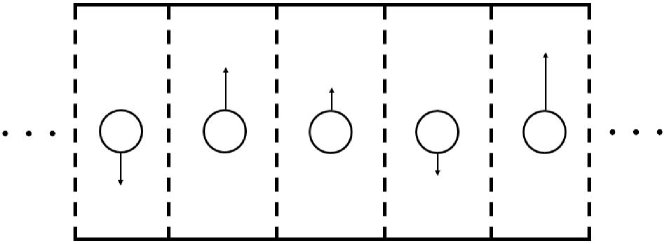
Figure 4.1: Sketch of the lattice model of granular media. Sites are characterized by a transverse-to-the-lattice velocity and exchange momentum and energy through nearest-neighbor collisions.

4.1.3 Average fields in the continuum limit

In the large system size limit as $L\to\infty$, a continuum limit may be introduced by considering that the average velocity $u_{l,p}=\langle v_{l,p}\rangle$ and energy $E_{l,p}=\langle v_{l,p}^{2}\rangle$ are smooth functions of space and time. Of course, the local temperature $T_{l,p}=E_{l,p}-u_{l,p}^{2}$ is also assumed to be smooth. Specifically, we introduce hydrodynamic continuous space and time variables, respectively,

$$x=\frac{l-1}{L},\quad t=\frac{\omega\tau}{L^{2}}.$$ (4.9)

For $\beta=0$, the balance equations for the average velocity $u(x,t)$ and energy

$$E(x,t)=u^{2}(x,t)+T(x,t)$$ (4.10)

read

$$\partial_{t}u(x,t) =-\partial_{x}j_{\text{av}}(x,t),$$ (4.11a)

$$\partial_{t}E(x,t) =-\partial_{x}J_{\text{av}}(x,t)+d_{\text{av}}(x,t).$$ (4.11b)

Therein, the average momentum and energy currents, $j_{\text{av}}(x,t)$ and $J_{\text{av}}(x,t)$, respectively, are given by

$$j_{\text{av}}(x,t)=-\partial_{x}u(x,t),\quad J_{\text{av}}(x,t)=-\partial_{x}E(x,t),$$ (4.12)

and the dissipation field $d_{\text{av}}(x,t)$ is

$$d_{\text{av}}(x,t)=-\nu T,$$ (4.13)

with

$$\nu=(1-\alpha^{2})L^{2}.$$ (4.14)

In order to write the average dissipation we have made use of the molecular chaos assumption or Stosszahlansatz. Specifically, we have assumed that

$$\langle v_{l,p}v_{l\pm 1,p}\rangle=u_{l,p}u_{l\pm 1,p}+\mathcal{O}(L^{-1}).$$ (4.15)

In (4.14), we have introduced the macroscopic dissipation coefficient $\nu$, which is the relevant parameter in the hydrodynamic space and time scales [150, 151]. Note that if $\nu$ is of order unity, the collisions have to be quasi-elastic $1-\alpha^{2}\ll 1$. It is straightforward to combine (4.11), (4.12) and (4.13) to write closed equations for the hydrodynamic fields: average velocity and temperature,

$$\partial_{t}u(x,t) =\partial_{xx}u(x,t),$$ (4.16a)

$$\partial_{t}T(x,t) =-\nu T(x,t)+\partial_{xx}T(x,t)+2\left[\partial_{x}u(x,t)\right]^{2}.$$ (4.16b)

These equations must be solved submitted to suitable boundary conditions, which depend on the physical state under scrutiny. Note the resemblance between our hydrodynamic equations and those in (1.13).

4.1.4 Fluctuating hydrodynamics

The balance equations (4.11) may also be written at the fluctuating level of description, by considering that $v(x,t)$ and $e(x,t)$ are fluctuating quantities, whose averages are $u(x,t)$ and $E(x,t)$. In this way, fluctuating balance equations are written for both $v(x,t)$ and $e(x,t)$, which are the continuum limit versions of the microscopic balance equations (4.4) and (4.5), namely

$$\partial_{t}{v}(x,t)=-\partial_{x}j(x,t), j(x,t)=-\partial_{x}v(x,t)+\xi^{(j)}(x,t),$$ (4.17a)

$$\partial_{t}{e}(x,t)=-\partial_{x}J(x,t)+d(x,t), J(x,t)=-\partial_{x}e(x,t)+\xi^{(J)}(x,t).$$ (4.17b)

In the equations above, $(j,J)$ are the fluctuating currents for momentum and energy, and $(\xi^{(j)},\xi^{(J)})$ are their corresponding noises. These noises have been shown to be Gaussian and white [150, 151]. The amplitudes of their correlations $\langle\xi^{(\gamma)}\xi^{(\gamma^{\prime})}\rangle$ can be cast in matrix form,

$$\langle\xi^{(\gamma)}(x,t)\xi^{(\gamma^{\prime})}(x^{\prime},t^{\prime})\rangle=L^{-1}\bm{\Xi}^{(\gamma\gamma^{\prime})}\delta(x-x^{\prime})\delta(t-t^{\prime}),$$ (4.18)

where $(1,2)$ for $\gamma$ or $\gamma^{\prime}$ correspond to $(j,J)$. These amplitudes have been computed within the local equilibrium approximation in [150], with the result

$$\bm{\Xi}=2T(x,t)\begin{pmatrix}1&&2u(x,t)\\ 2u(x,t)&&2[T(x,t)+2u^{2}(x,t)]\end{pmatrix}.$$ (4.19)

The average velocity $u(x,t)$ and the temperature $T(x,t)$ must be calculated in the state corresponding to the physical situation of interest.

Finally, the dissipation field $d(x,t)$ is given by

$$d(x,t)=-\nu\theta(x,t)=-\nu\left[e(x,t)-v_{R}^{2}(x,t)\right],$$ (4.20)

where $v_{R}^{2}$ is the regular part of $v^{2}$, defined as

$$v_{R}^{2}(x,t)\equiv v^{2}(x,t)-L^{-1}\theta(x,t)\lim_{\Delta x\to 0}\delta(\Delta x).$$ (4.21)

This regular part of the velocity field has the property $\langle v_{R}^{2}(x,t)\rangle=u^{2}(x,t)$, as shown in appendix B. Equation (4.20) tells us that the fluctuations of the dissipation field are enslaved to those of the fluctuating temperature field $\theta(x,t)$. This is so because the dissipation noise $\xi^{(d)}$ is subdominant as compared to the current noises, since it scales as $L^{-3}$ instead of as $L^{-1}$, as proven in [150].

4.2 Dynamics of the one-particle distribution function

Here, we apply the usual procedure of kinetic theory and map the master equation into a BBGKY hierarchy. In particular, we focus on the evolution equation for the one-particle distribution function at site $l$ and at time $\tau$, which we denote by $P_{1}(v;l,\tau)$. By definition,

$$P_{1}(v;l,\tau)=\int d\bm{v}P_{N}(\bm{v},\tau)\delta(v_{l}-v).$$ (4.22)

It is easy to show that none of the terms in the sum (4.7) contribute to the time evolution of $P_{1}$ except those corresponding to $l-1$ and $l$, because the collisions involving the pairs $(l-1,l)$ and $(l,l+1)$ are the only ones which change the velocity at site $l$. Therefore,

$$\partial_{\tau}P_{1}(v;l,\tau)=\omega$$

$$\times\left\{\int_{-\infty}^{+\infty}\!\!dv_{l-1}|\Delta_{l-1}|^{\beta}\left[\frac{P_{2}(\hat{b}_{l-1}^{-1}\{v_{l-1},v\};l-1,l,\tau)}{\alpha^{\beta+1}}-P_{2}(v_{l-1},v;l-1,l,\tau)\right]\right.$$

$$\left.\;+\int_{-\infty}^{+\infty}\!\!dv_{l+1}|\Delta_{l}|^{\beta}\left[\frac{P_{2}(\hat{b}_{l}^{-1}\{v,v_{l+1}\};l,l+1,\tau)}{\alpha^{\beta+1}}-P_{2}(v,v_{l+1};l,l+1,\tau)\right]\right\},$$

where $P_{2}(v,v^{\prime};l,l+1,\tau)$ is the two-particle probability distribution for finding the particles at the $l$-th and $(l+1)$-th sites with velocities $v$ and $v^{\prime}$, respectively. For the special case $\beta=0$, the evolution equation for $P_{1}$ can be further simplified, because the terms on the rhs of (4.2) coming from the loss (negative) terms of the master equation can be integrated. We get

$$\partial_{\tau}P_{1}(v;l,\tau)=\omega\left[-2P_{1}(v;l,\tau)+\frac{1}{\alpha}\int_{-\infty}^{+\infty}dv_{l-1}P_{2}(\hat{b}_{l-1}^{-1}\{v_{l-1},v\};l-1,l,\tau)\right.\\ +\left.\frac{1}{\alpha}\int_{-\infty}^{+\infty}dv_{l+1}P_{2}(\hat{b}_{l}^{-1}\{v,v_{l+1}\};l,l+1,\tau)\right].$$ (4.24)

The equation for $P_{1}$, either (4.2) for a generic $\beta$ or (4.24) for $\beta=0$, could be converted to a closed equation for $P_{1}$ by introducing the molecular chaos assumption, which in our present context means that

$$P_{2}(v,v^{\prime};l,l+1,\tau)=P_{1}(v;l,\tau)P_{1}(v^{\prime};l+1,\tau)+\mathcal{O}(L^{-1}).$$ (4.25)

By neglecting the $\mathcal{O}(L^{-1})$ terms in (4.25), we obtain a pseudo-Boltzmann or kinetic equation for $P_{1}$, which determines the evolution of the one-time and one-particle averages under the assumption of $\mathcal{O}(L^{-1})$ correlations. Note that this “smallness” of two-particle correlations do not prevent them from being long-ranged.

In the continuum (hydrodynamic-like) limit defined in (4.9), the evolution equation for the one-particle distribution function (4.2) can be written in a simpler form. The main idea is the quasi-elasticity of the microscopic dynamics, stemming from (4.14), i.e. $\alpha=1-L^{-2}\nu/2+\mathcal{O}(L^{-4})$. Then,

$$P_{2}\left(\hat{b}^{-1}_{l-1}\{v_{l-1},v\};l-1,l,\tau\right)=P_{2}\left(v-\frac{\nu}{4L^{2}}\Delta_{l-1},v_{l-1}+\frac{\nu}{4L^{2}}\Delta_{l-1};l-1,l,\tau\right)$$

$$=\left[1+\frac{\nu}{4L^{2}}\Delta_{l-1}(\partial_{v_{l-1}}-\partial_{v})\right]P_{2}(v,v_{l-1};l-1,l,\tau)+\mathcal{O}(L^{-4}).$$ (4.26)

Moreover, we make use of the molecular chaos assumption (4.25) and identify

$$P_{1}(v;l,\tau)=P_{1}(v;x=(l-1)/L,t=\omega\tau/L^{2}),$$ (4.27)

that is, we consider $P_{1}$ to be a smooth function of the hydrodynamic space and time variables $x$ and $t$.

Under the hypotheses outlined above, a lengthy but straightforward calculation gives for arbitrary $\beta$ that

$$\partial_{t}P_{1}(v;x,t)= \,\,\partial_{x}\int_{-\infty}^{+\infty}dv^{\prime}|v^{\prime}-v|^{\beta}\left[P_{1}(v^{\prime};x,t)\partial_{x}P_{1}(v;x,t)\right.$$

$$\qquad\qquad\qquad\qquad\qquad-\left.P_{1}(v;x,t)\partial_{x}P_{1}(v^{\prime};x,t)\right]$$

$$-\frac{\nu}{2}\partial_{v}\int_{-\infty}^{+\infty}dv^{\prime}(v^{\prime}-v)|v^{\prime}-v|^{\beta}P_{1}(v^{\prime};x,t)P_{1}(v;x,t).$$ (4.28)

The most important corrections to this equation emanate from finite size effects that give rise to nonzero correlations, i.e. the corrections to molecular chaos hypothesis that are expected to be of the order of $L^{-1}$, see section 4.5 for details. This equation must be supplemented with suitable boundary conditions depending on the physical state under scrutiny. Note that the divergence structure of the rhs of (4.2) stems from the fact that $P_{1}(v;x,t)$ is a locally conserved quantity.

If we took moments in (4.2), we would obtain the hydrodynamic equations for a generic value of $\beta$. It is clear, from the structure of this equation, that these hydrodynamic equations would be not closed and constitutive relations for the momentum and energy currents and the dissipation fields would be needed. We also recall that in our model there is no mass transport and therefore the “field density” $n(x,t)$ is uniform and constant in time,

$$n(x,t)=\int_{-\infty}^{+\infty}dv\,P_{1}(v;x,t)=1,$$ (4.29)

which is consistent with the result $\partial_{t}n(x,t)=0$ obtained by marginalizing $v$ in (4.2).

Again, for the case $\beta=0$, the equation for $P_{1}$ in the continuum limit can be simplified,

$$\partial_{t}P_{1}(v;x,t)=\partial_{xx}P_{1}(v;x,t)+\frac{\nu}{2}\partial_{v}\left[(v-u(x,t))P_{1}(v;x,t)\right]$$ (4.30)

The above equation is not linear for $P_{1}$, since the average momentum is a functional thereof, $u(x,t)=\int_{-\infty}^{+\infty}dv\,vP_{1}(v;x,t)$. Note that, consistently, by taking moments in (4.30), the average hydrodynamic equations (4.16) are reobtained. Moreover, the evolution equations for all the moments are closed (at any order) under the molecular chaos assumption, without further knowledge of the one-particle distribution function $P_{1}$.

Note that an appealing physical picture for $P_{1}(v;x,t)$ arises in the continuum limit. In fact,

$$P_{1}(v;x,t)\,dv\,dx=\sum_{l=1}^{N}P_{1}(v;l,t)\,dv\,\Delta x\,\Theta(L^{-1}l-x)\Theta(x+dx-L^{-1}l)\\ =L^{-1}\sum_{l=1}^{N}P_{1}(v;l,t)\,dv\,\Theta(L^{-1}l-x)\Theta(x+dx-L^{-1}l),$$ (4.31)

in which $\Theta(x)$ is Heaviside step function. The product of Heaviside functions selects the range of $l$’s corresponding to the interval $(x,x+dx)$. Thus, $P_{1}(v;x,t)dv\,dx$ can be interpreted as the fraction of the total number of particles with velocities in the interval $(v,v+dv)$ and positions in the interval $(x,x+dx)$, which makes it neater the connection with the usual kinetic approach.

4.3 The one-particle distribution function for some physical states

In this section, we restrict ourselves to the pseudo-Maxwell case $\beta=0$. Therein, we analyze two physically relevant states that are typical of dissipative systems such as granular fluids. Specifically, we investigate the Homogeneous Cooling State (HCS) and the Uniform Shear Flow (USF) state. Although the model also admits stationary solutions of Couette Flows for appropiate boundary conditions [150, 151], they are not treated here. The theoretical results below are compared to numerical results, which have been obtained by means of Monte Carlo simulations described in appendix C. Specifically, we always plot the scaled one-particle distribution defined as

$$\varphi(c;x,t)=\sqrt{T(x,t)}P_{1}(v;x,t),\quad c=\frac{v-u(x,t)}{\sqrt{T(x,t)}},$$ (4.32)

in order to avoid visualizing the much sharper distributions $P_{1}$ that arise in some situations as a consequence of the cooling.

4.3.1 The Homogeneous Cooling State

Let us consider a system with periodic boundary conditions. Moreover, the initial condition is “thermal”, that is, the random variables $v_{l,0}$ are Gaussian with zero average and unit variance. This means that we are choosing the uniform initial temperature to be the temperature unit. From this initial condition, the system evolves into the state known as the Homogeneous Cooling State (HCS), in which the system remains homogeneous and the temperature decays in time. At the (average) hydrodynamic level, one has [150, 151]

$$u(x,t)=0,\qquad T_{\text{\tiny HCS}}(x,t)=T(t=0)e^{-\nu t}.$$ (4.33)

Since the collision frequency of our model is velocity-independent, we are dealing with pseudo-Maxwell molecules and thus the temperature decays exponentially in time. This is the expected behavior, which replaces the typical algebraic decay for hard particles, known as Haff’s law [81].

As stated in 1.2.1, the HCS is known to be unstable: it breaks down in too large or too inelastic systems [85, 62]. In our model and in the continuum limit, this condition (studied in [79]) reads $\nu>\nu_{c}$, or, equivalently, $L>L_{c}$, where

$$\nu_{c}=8\pi^{2},\quad L_{c}=2\pi\sqrt{2}\left(1-\alpha^{2}\right)^{-1/2}.$$ (4.34)

Note that the scaling of the critical length $L_{c}$ is the same as that introduced in (1.12). When $\nu<\nu_{c}$ (or $L<L_{c}$) there is no unstable mode. This instability mechanisms is completely analogous to the one found in granular gases for the shear mode [156]. Note that the amplification appears in the rescaled velocity $\tilde{u}(x,t)=u(x,t)/v_{\text{th}}(t)$, being $v_{\text{th}}(t)=\sqrt{T_{\text{\tiny HCS}}(t)}$, and not in the velocity $u(x,t)$.

Interestingly, the one-particle distribution function can be exactly calculated in the HCS. Taking into account the homogeneity of the state and the vanishing of the average velocity $u(x,t)$, (4.30) for $P_{1}(v;t)$ simplifies to

$$\partial_{t}P_{1}(v;t)=\frac{\nu}{2}\partial_{v}\left[vP_{1}(v;t)\right].$$ (4.35)

This equation can be integrated right away to give

$$P_{1}(v;t)=e^{\nu t/2}P_{1}(ve^{\nu t/2};t=0).$$ (4.36)

Now, we employ the definition of the scaled distribution function (4.32), that here reduces to

$$\varphi(c;t)=v_{\text{th}}(t)P_{1}(v;t),\quad c=v/v_{\text{th}}(t).$$ (4.37)

By combining (4.36) and (4.37), we find that $\varphi(c;t)$ does not evolve, that is,

$$\varphi(c;t)=\sqrt{T(0)}P_{1}(c\sqrt{T(0)};t=0)=\varphi(c;0).$$ (4.38)

Therefore, the one-particle distribution function would remain Gaussian for all times if it were so initially, as is usually the case. In general, the shape of the initial distribution of velocities is not altered, and it only “shrinks” with the thermal velocity. A similar behavior was found for elastic Maxwell molecules with annihilation starting from the Boltzmann equation [157]. This is a peculiarity of Maxwell molecules, in which the probability that a given pair collides is independent of its relative velocity.

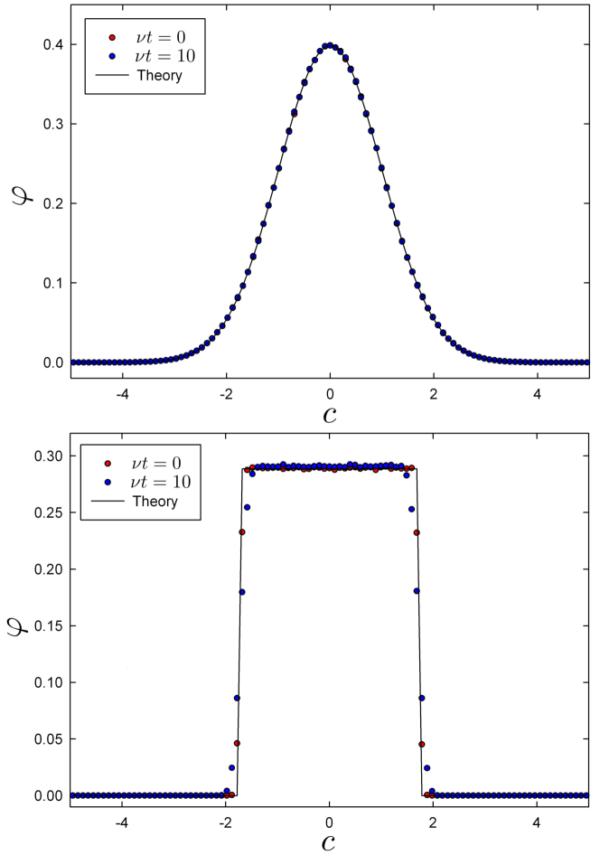
Figure 4.2: Time evolution of the scaled one-particle distribution function $\varphi(c)$ in the HCS. The shape of the distribution remains unaltered when plotted as a function of the scaled velocity $c=v/v_{\text{th}}(t)$. The two panels correspond to different initial conditions $P_{1}(v;0)$: Gaussian (top) and square (bottom). Note that deviations from the initial shape are barely observable in the Gaussian case, and remain very small for the square shape. We have averaged over $10^{4}$ realizations, in a system with $N=500$ and $\nu=20$.

We have simulated the homogeneous cooling state of a system made of $10^{3}$ particles, with periodic boundaries and starting from a flat velocity profile $u(x,0)\equiv 0$ with unit variance $T(x,0)\equiv T_{0}=1$. It can be observed how the one-particle distribution function $P_{1}(v;t)$ conserves its initial shape, as given by (4.38). We check numerically this result for $\nu=20$ by considering two initial velocity distributions, Gaussian and square, that is,

$$P_{1}(v;t=0)=(2v_{0})^{-1}\Theta(v_{0}-|v|),$$ (4.39)

$\Theta(v)$ being the Heaviside step function. The parameter $v_{0}$ is adjusted in order to have unit variance ($v_{0}=\sqrt{3}$). In figure 4.2, we compare the theoretical prediction with numerical results, finding excellent agreement except for very small finite-size corrections.

4.3.2 The Uniform Shear Flow steady state

Here, a velocity difference $a$ (shear rate) is imposed between the velocities at the left and right boundaries of the system. Specifically, the boundary conditions for the hydrodynamic equations are

$$u(1,t)-u(0,t) =a,\; \left.\partial_{x}u(x,t)\right|_{x=0} =\left.\partial_{x}u(x,t)\right|_{x=1},$$ (4.40a)

$$T(0,t) =T(1,t),\; \left.\partial_{x}T(x,t)\right|_{x=0} =\left.\partial_{x}T(x,t)\right|_{x=1},$$ (4.40b)

that is, of Lees-Edwards type [158]. The corresponding stationary solution of the hydrodynamic equations (4.16) is known as the Uniform Shear Flow (USF) state,

$$u_{s}(x)=a(x-1/2),\quad T_{s}=2a^{2}/\nu,$$ (4.41)

that is, the velocity profile is linear whereas the temperature remains homogeneous. This steady state is peculiar of dissipative systems, the continuous energy loss in collisions compensates the viscous heating. The rheological effects described by Santos et al. [159, 160] are not present in our system because the microscopic dynamics is quasi-elastic.

In chapter 5, we show that the USF is globally stable, that is, the system monotonically approaches the USF state from any initial condition. This is done by proving an $H$-theorem [95, 161] at the level of the one-particle distribution function. Physically, this is reasonable because the energy injection allows the system to fully explore its phase space, which hints at the validity of the $H$-theorem for the master equation at the $N$-particle level [97, 98]. This is consistent with the (linear) stability of the USF state of a dilute granular gas of hard spheres [86] with respect to perturbations in the velocity gradient introduced in section 1.2.1. Note that in our 1d model mimicking the shear modes, these perturbations are the only possible ones to consider.

For the USF state, the stationary solution of the one-particle distribution function can be solved: we seek a time-independent solution of (4.30) with the “scaling” form

$$P_{1}^{(\text{s})}(v;x)=T_{s}^{-1/2}\varphi(c),\qquad c=\frac{v-u_{s}(x)}{T_{s}^{1/2}}.$$ (4.42)

By doing so, the probability distribution verifies the appropriate boundary conditions for the USF state, that is,

$$P_{1}(v;x=1,t)=P_{1}(v-a;x=0,t),\quad\left.\partial_{x}P_{1}(v;x,t)\right|_{x=1}=\left.\partial_{x}P_{1}(v-a;x,t)\right|_{x=0}.$$ (4.43)

Therefrom, the Lees-Edwards conditions directly follow (4.40). The resulting equation for $\varphi(c)$ is

$$\varphi^{\prime\prime}(c)+[c\varphi(c)]^{\prime}=0,$$ (4.44)

in which the prime stands for the derivative with respect to $c$. Thus, the physical solution is $\varphi(c)\propto\exp(-c^{2}/2)$ and

$$P_{1}^{(\text{s})}(v;x)=(2\pi T_{s})^{-1/2}\exp\left\{-\frac{[v-u_{s}(x)]^{2}}{2T_{s}}\right\},$$ (4.45)

that is, the steady one-particle velocity distribution for the USF state is a Gaussian with average local velocity $u_{s}(x)$ and temperature $T_{s}$. In [150, 151], the equation for higher order central moments of the velocity have been derived. Of course, the steady values for those moments are in agreement with the Gaussian shape obtained here.

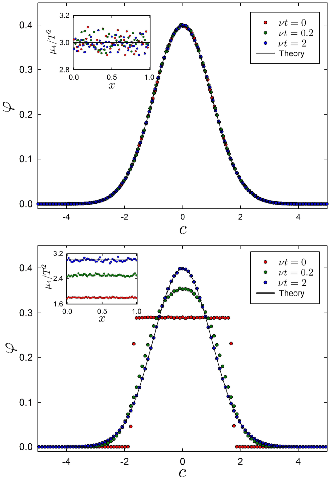
Figure 4.3: Evolution of the scaled one-particle velocity distribution in the USF. Specifically, we show how the Gaussian steady distribution (4.45) is approached. In both panels, the initial velocity profile is already the steady one $u_{s}(x)$ but the initial homogeneous temperature $T_{0}=1\neq T_{s}$. We have considered, a shear rate $a=5$ in a system with $N=500$ and $\nu=20$. Different initial shapes of the distribution have been chosen for each panel: Gaussian (top) and square (bottom). In the insets, we show the time evolution of the fourth central moment $\mu_{4}$ over $T^{2}$, which equals 3 for a Gaussian distribution, In all cases, averages over $M=10^{4}$ simulation trajectories have been performed.

The USF described above can be simulated by introducing appropriate collision rules for the boundary pairs. When the pair $(1,N)$ is chosen to collide at time $p$, there are two separate collisions: particle $1$ ($N$) undergoes a collision with a particle with velocity $v_{N,p}-a$ ($v_{1,p}+a$). These boundary collision rules introduce a shear rate $a$ between the left and right ends of the system, and at the hydrodynamic level are represented by the Lees-Edwards conditions (4.40). This can be readily shown by considering the special evolution equations for $v_{1,p}$ and $v_{N,p}$ with the above boundary collision rules in the continuum limit, see appendix D.

In figure 4.3, we check numerically the tendency of the system to approach the steady Gaussian one-particle velocity distribution of the USF state, given by (4.45). We do so in two cases: in the top panel, we start from a Gaussian distribution with the steady velocity profile but with an initial value of the temperature $T_{0}=1\neq T_{s}$. No time evolution is apparent in the scaled variables, since the distribution remains a Gaussian of unit variance for all times. In the bottom panel, our simulation starts from a square distribution. It is clearly observed that the Gaussian shape is approached as time increases. In the inset of both panels, we show the fourth central moment $\mu_{4}$ over $T^{2}$ at the same times, which also tends to its Gaussian value.

For the longest time in figure 4.3, $\nu t=2$, the one-particle velocity distribution has already reached the predicted Gaussian shape. It is worth pointing out that this is so although the temperature is still $10$% below its steady value (not shown, see [150, 151]). This fact suggests the existence of a two-step approach to the steady state. In a first stage, the one-particle distribution function forgets its initial conditions and tends to a “normal” solution of the kinetic equation. Afterwards, it is moving over this “normal” solution that the system reaches the steady state. This resembles the so-called hydrodynamic $\beta$-state reported by García de Soria et al. in a uniformly heated granular gas [162, 163].

4.4 Study of the fluctuations

In this section, we focus on fluctuations around the HCS, which have already been analyzed in the literature for a hard-sphere system described by the Boltzmann equation close to the shear instability [164]. To do so, it is useful to go to Fourier space, by considering that all the fields are written as

$$y(x,t)=\sum_{n}y_{n}(t)e^{ik_{n}x},\quad y_{n}(t)=\int_{0}^{1}dx\,y(x,t)e^{-ik_{n}x},\;k_{n}=2n\pi.$$ (4.46)

4.4.1 Velocity fluctuations

The equation for the fluctuating velocity (4.17a) is closed,

$$\partial_{t}{v}=\partial_{xx}v-\partial_{x}\xi^{(j)},$$ (4.47)

and going to Fourier space,

$$\partial_{t}{v}_{n}=-k_{n}^{2}v_{n}-ik\xi_{n}^{(j)}.$$ (4.48)

The long time behavior of the solution to (4.48) is readily obtained by taking the initial time $t_{0}$ to $-\infty$, and then

$$v_{n}(t)=-ik_{n}\int_{-\infty}^{t}ds\,e^{-k_{n}^{2}(t-s)}\xi_{n}^{(j)}(s).$$ (4.49)

Now, we compute the equal-time velocity correlation in Fourier space,

$$\langle v_{n}(t)v_{n^{\prime}}(t)\rangle_{\text{\tiny HCS}}=-k^{2}\int_{-\infty}^{t}\!\!\!ds\,e^{-k^{2}(t-s)}\int_{-\infty}^{t}\!\!\!ds^{\prime}e^{-k^{2}(t-s^{\prime})}\langle\xi_{n}^{(j)}(s)\xi_{n^{\prime}}^{(j)}(s^{\prime})\rangle_{\text{\tiny HCS}}.$$ (4.50)

Making use of the time dependence of the temperature in the HCS, that is, Haff’s law (4.33), we get to the lowest order

$$\langle v_{n}(t)v_{n^{\prime}}(t)\rangle_{\text{\tiny HCS}}=\frac{T_{\text{\tiny HCS}}(t)}{L}\frac{2k_{n}^{2}}{2k_{n}^{2}-\nu}\delta_{n,-n^{\prime}}=\frac{T_{\text{\tiny HCS}}(t)}{L}\left(1+\frac{\nu}{2k_{n}^{2}-\nu}\right)\delta_{n,-n^{\prime}},$$ (4.51)

provided that $2k_{n}^{2}-\nu>0$. Thus, these correlations are valid for all $n$ when $\nu<\nu_{c}=8\pi^{2}$ since at $\nu=\nu_{c}$ we have that $\langle v_{1}(t)v_{-1}(t)\rangle$ diverges.

The above correlations allow us to calculate the spatial integral of $v^{2}(x,t)$. At the fluctuating level, we have that

$$\int_{0}^{1}dx\,v^{2}(x,t)=\sum_{n=-\infty}^{+\infty}v_{n}(t)v_{-n}(t),$$ (4.52)

which is Parseval’s theorem for the Fourier transform. By taking averages, we readily see that $v^{2}$ has a singular contribution, because the sum of the correlations $\langle v_{n}(t)v_{-n}(t)\rangle$ diverges. This stems from the $\delta(0)$ contribution in (4.21), the average value of which in the HCS is

$$\langle L^{-1}\theta(x,t)\lim_{\Delta x\to 0}\delta(\Delta x)\rangle=L^{-1}T_{\text{\tiny HCS}}(t)\sum_{n}1,$$ (4.53)

since $\delta(x-x^{\prime})=\sum_{n}\exp[ik_{n}(x-x^{\prime})]$. Therefore,

$$\hskip 34.1433pt\int_{0}^{1}dx\,\langle v_{R}^{2}(x,t)\rangle =\frac{T_{\text{\tiny HCS}}(t)}{L}\,\psi_{\text{\tiny HCS}},$$ (4.54a)

$$\psi_{\text{\tiny HCS}}(\nu)\equiv\sum_{n}\frac{\nu}{2k_{n}^{2}-\nu} =-\frac{\sqrt{\nu}}{2\sqrt{2}}\cot\left({\frac{\sqrt{\nu}}{2\sqrt{2}}}\right).$$ (4.54b)

Of course, the spatial integral of the regular part has a finite value. The shear instability of the HCS is clearly observed within the framework of the fluctuating hydrodynamic description: at $\nu=\nu_{c}=8\pi^{2}$, we have that

$$\lim_{\nu\to\nu_{c}}\psi_{\text{\tiny HCS}}(\nu)=\infty,$$ (4.55)

and the spatial integral of $v_{R}^{2}$ diverge. In particular, it is $\langle v_{1}(t)v_{-1}(t)\rangle$ that diverges, as readily seen from (4.51) and said above.

4.4.2 Effect of velocity fluctuations on the total energy

Here, we consider the fluctuations of the total energy per particle, defined by

$$e(t)=\int_{0}^{1}dx\,e(x,t).$$ (4.56)

At the mesoscopic fluctuating level, we have that

$$\frac{d}{dt}e(t)=\int_{0}^{1}dx\,d(x,t)=-\nu\,e(t)+\nu\!\int_{0}^{1}dx\,v_{R}^{2}(x,t),$$ (4.57)

consistently with (4.17) and (4.20).

We introduce a rescaled dimensionless total energy by

$$\tilde{e}(t)=\frac{e(t)}{T_{\text{\tiny HCS}}(t)},$$ (4.58)

which verifies the evolution equation

$$\frac{d}{dt}\tilde{e}(t)=\nu\!\int_{0}^{1}dx\,\tilde{v}_{R}^{2}(x,t),$$ (4.59)

in which $\tilde{v}_{R}^{2}(x,t)=v_{R}^{2}(x,t)/T_{\text{\tiny HCS}}(t)$. Now, we take averages and make use of (4.54) to write

$$\frac{d}{dt}\tilde{E}(t)=\psi_{\text{\tiny HCS}}\frac{\nu}{L},$$ (4.60)

which has to be integrated with the initial condition $\tilde{E}(0)=1$. We have omitted the $\nu$-dependence of $\psi_{\text{\tiny HCS}}$ in order not to clutter our formulae. Therefore, up to order of $L^{-1}$, we have

$$\tilde{E}(t)=1+\delta\tilde{E}(t),\quad\delta{\tilde{E}}(t)=\psi_{\text{\tiny HCS}}\frac{\nu\,t}{L}.$$ (4.61)

which is expected to be valid as long as $\nu\psi_{\text{\tiny HCS}}t/L\ll 1$. Equation (4.61) can be also obtained by solving perturbatively the evolution equations for the temperature and two-particle correlation function [155, 151].

There is a critical dissipation value $\nu_{\psi}$ such that $\psi_{\text{\tiny HCS}}$ vanishes, that is,

$$\nu_{\psi}=\nu_{c}/4=2\pi^{2},\qquad\psi_{\text{\tiny HCS}}(\nu_{\psi})=0,$$ (4.62)

and the finite-size correction in (4.61) changes sign. Therefore, at this point we find a change in the time-derivative of $\delta\tilde{E}(t)$. For large system sizes, the energy decays faster (slower) than the Haff’s law for $\nu<\nu_{\psi}$ ($\nu>\nu_{\psi}$) because $\psi_{\text{\tiny HCS}}<0$ ($\psi_{\text{\tiny HCS}}>0$). Comparisons between these theoretical results and Monte Carlo simulations give an excellent agreement [155, 151].

4.5 Finite size effects: exact solution of the HCS

In this section, we further analyze the velocity correlations. The average equation for the granular temperature (or the energy) in the HCS is closed only when the correlation $\langle v_{l}v_{l+1}\rangle$ is neglected, since it is expected to be of the order of $L^{-1}$. In other words, the evolution equation for the temperature is closed in the molecular chaos approximation. Interestingly, for the case of Maxwell molecules we are considering in this work, we can account for the effect of the correlations in an exact way, thus going beyond molecular chaos.

We assume that the system is in a spatial-translation-invariant state, such as the HCS. We define the set of spatial correlations of the velocity at time $\tau$ as

$$C_{k}(\tau)=\langle v_{j}(\tau)v_{j+k}(\tau)\rangle.$$ (4.63)

Here, $k$ represents the distance between the involved sites in the correlation. Note that the average temperature at any site $j$ is given by $C_{0}$,

$$T(\tau)\equiv C_{0}(\tau)=\langle v_{j}^{2}(\tau)\rangle.$$ (4.64)

As a consequence of momentum conservation, in the center of mass frame we have the “sum rule”

$$C_{0}(\tau)+2\sum_{k=1}^{\frac{L-1}{2}}C_{k}(\tau)=0,\quad\forall\tau,$$ (4.65)

where we have considered an odd $L$.

The evolution equation of the correlations is readily obtained from the master equation (4.7),

$$\omega^{-1}\partial_{\tau}{C_{0}}= \,\,(\alpha^{2}-1)(C_{0}-C_{1}),$$ (4.66a)

$$\omega^{-1}\partial_{\tau}{C_{1}}= \,\,\frac{1-\alpha^{2}}{2}(C_{0}-C_{1})+(1+\alpha)(C_{2}-C_{1}),$$ (4.66b)

$$\omega^{-1}\partial_{\tau}{C_{k}}= \,\,(1+\alpha)(C_{k+1}+C_{k-1}-2C_{k}),\quad 2\leq k\leq(L-1)/2,$$ (4.66c)

$$\hskip 19.91692ptC_{\frac{L+1}{2}}= \,\,C_{\frac{L-1}{2}},\quad\forall\tau.$$ (4.66d)

Above, we have omitted the $\tau$-dependence of the correlations to keep our notation simple, and written the evolution equations for odd $L$, because the “upper” boundary condition (for the maximum value of $k$) is simpler to write. For even $L$, the boundary condition would read $C_{\frac{L}{2}+1}=C_{\frac{L}{2}-1}$. Of course, our choice of $L$ as odd is irrelevant in the large system size limit $L\gg 1$.

The hierarchy (4.66) can be exactly solved by reducing it to the eigenvalue problem of a certain matrix. We carry out this approach to the problem also for odd $L$. The problem for an even number particles may be solved by following an utterly similar strategy, but the boundary conditions are a little more involved to write. We do not present here these calculations because they do not provide any additional physical insight.

First, it is useful to introduce a change of variables in order to make the matrix symmetric. Specifically, we define

$$c_{0}=C_{0},\qquad c_{k}=\sqrt{2}\,C_{k},\quad 1\leq k\leq(L-1)/2.$$ (4.67)

Second, we rewrite the hierarchy (4.66) as

$$\omega^{-1}(1+\alpha)^{-1}\partial_{\tau}c_{0} =-(1-\alpha)c_{0}+\frac{1-\alpha}{\sqrt{2}}c_{1},$$ (4.68a)

$$\omega^{-1}(1+\alpha)^{-1}\partial_{\tau}c_{1} =\frac{1-\alpha}{\sqrt{2}}c_{0}-\frac{3-\alpha}{2}c_{1}+c_{2},$$ (4.68b)

$$\omega^{-1}(1+\alpha)^{-1}\partial_{\tau}c_{k} =c_{k-1}-2c_{k}+c_{k+1},\quad 2\leq k\leq(L-3)/2,$$ (4.68c)

$$\omega^{-1}(1+\alpha)^{-1}\partial_{\tau}c_{\frac{L-1}{2}} =c_{\frac{L-3}{2}}-c_{\frac{L-1}{2}},$$ (4.68d)

in which we have extracted the common factor $(1+\alpha)$ on the rhs of (4.66) and made use of (4.66d) to write (4.68d) for $c_{\frac{L-1}{2}}$.

Now, we can solve the system above by a standard eigenvector method, that is, we seek solutions of the form

$$c_{k}=e^{\lambda(1+\alpha)\omega\tau}\phi_{k}.$$ (4.69)

We denote the eigenvalues by $\lambda$ and its corresponding eigenvector by $\phi$, $\phi_{k}$ is thus the $k$-th component thereof. In this way, we reach the system

$$\hskip 8.53581pt\lambda\phi_{0} =-(1-\alpha)\phi_{0}+\frac{(1-\alpha)}{\sqrt{2}}\phi_{1},$$ (4.70a)

$$\hskip 8.53581pt\lambda\phi_{1} =\frac{(1-\alpha)}{\sqrt{2}}\phi_{0}-\frac{(3-\alpha)}{2}\phi_{1}+\phi_{2},$$ (4.70b)

$$\hskip 8.53581pt\lambda\phi_{k} =\phi_{k-1}-2\phi_{k}+\phi_{k+1},\quad 2\leq k\leq(L-3)/2,$$ (4.70c)

$$\lambda\phi_{\frac{L-1}{2}} =\phi_{\frac{L-3}{2}}-\phi_{\frac{L-1}{2}}.$$ (4.70d)

Equations (4.70) are a system of second-order difference equations for $\phi_{k}$ with constant coefficients, in which (4.70c) is the general equation and (4.70b) and (4.70d) are their boundary conditions. On top of that, (4.70a) acts as an extra condition that ensures momentum conservation, as shown below (see also [155, 151]). The general solution of (4.70c) is of the form $\phi_{k>0}=r^{k}$ [122], which substituted into (4.70c) has two solutions $(r_{1},r_{2})$ that verify

$$r_{1}r_{2} =1,$$ (4.71a)

$$r_{1}+r_{2} =2+\lambda.$$ (4.71b)

We introduce a new variable $q\in[0,\pi]$ such that $r_{1}=e^{iq}$ and $r_{2}=e^{-iq}$, as suggested by (4.71a). Note that $|r_{1}|=|r_{2}|=1$, if one of the roots were larger than one it would lead to correlations increasing with $k$, which is physically absurd. Moreover, from a purely mathematical point of view, restricting ourselves to $|r_{1}|=|r_{2}|=1$ leads to a complete set of eigenvectors. From (4.71b), we obtain

$$\lambda(q)=2(\cos q-1),$$ (4.72)

and the corresponding eigenvector is given by

$$\phi_{k>0}(q) =A\,e^{ikq}+B\,e^{-ikq},$$ (4.73a)

$$\phi_{0}(q) =\frac{1-\alpha}{\sqrt{2}\left(2\cos q-1-\alpha\right)}(A\,e^{iq}+B\,e^{-iq}).$$ (4.73b)

The boundary conditions (4.70b) and (4.70d) determine the constants $A$ and $B$, and also the allowed values of the “index” $q$. The determinant of the linear system for $A$ and $B$ must be zero, which is equivalent to impose that $q$ must be a zero of the function

$$g(q)= \,\,2\sin\left(\frac{L+3}{2}q\right)-(5+3\alpha)\sin\left(\frac{L+1}{2}q\right)+(5+7\alpha)\sin\left(\frac{L-1}{2}q\right)$$

$$-(3+5\alpha)\sin\left(\frac{L-3}{2}q\right)+(1+\alpha)\sin\left(\frac{L-5}{2}q\right).$$ (4.74)

This function has $(L+1)/2$ different zeros in the half-open interval $[0,\pi)$, which we denote by $q_{n}$: $q_{0}=0$, $q_{n}$ is the $n$-th nonvanishing zero of $g(q)$, $n=1,\ldots,(L-1)/2$. In addition $q=\pi$ also makes $g(q)$ vanish, but it does not correspond to an eigenvalue because the associated eigenvector would be identically zero, as shown below. In this way, we find $(L+1)/2$ eigenvalues

$$\lambda_{n}=2(\cos q_{n}-1),$$ (4.75)

the corresponding eigenvectors of which give a complete set for our problem. In figure 4.4, we plot the function $g(q)$ for $L=11$, which has six zeros in the interval $[0,\pi)$.

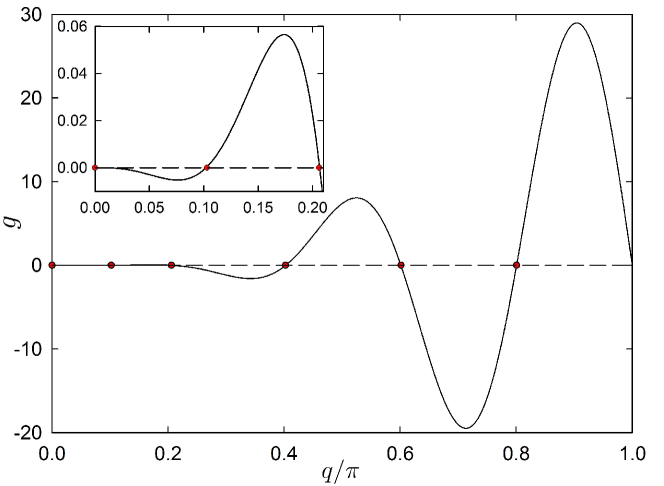
Figure 4.4: Plot of the function $g(q)$ defined in (4.5). The system size is $L=11$. Its zeros $q_{n}$ determine the eigenvalues, as given by (4.75). The first zero is always $q_{0}=0$, and there are $(L-1)/2$ additional zeros $q_{i}\neq 0$, $i=1,\ldots,(L-1)/2$. The inset shows a zoom of the small $q$ region, to facilitate the identification of $q_{1}$ and $q_{2}$.

The proportionality relation obtained between $A$ and $B$ makes it possible to write the eigenvector corresponding to the eigenvalue $\lambda_{n}$ up to a normalization constant $\mathcal{N}_{n}$,

$$\phi^{(n)}_{k>0} =\mathcal{N}_{n}\cos\left[\left(\frac{L}{2}-k\right)q_{n}\right],$$ (4.76a)

$$\phi^{(n)}_{0} =\frac{(1-\alpha)\mathcal{N}_{n}}{\sqrt{2}\left(2\cos q_{n}-1-\alpha\right)}\cos\left[\left(\frac{L}{2}-1\right)q_{n}\right].$$ (4.76b)

The above expressions clearly show that there is no eigenvector for $q=\pi$, since all its components are zero (recall that $L$ is odd). The constant $\mathcal{N}_{n}$ is chosen to obtain a orthonormal set of eigenvectors, in the sense that

$$\sum_{k=0}^{\frac{L-1}{2}}\phi^{(n)}_{k}\phi^{(n^{\prime})}_{k}=\delta_{nn^{\prime}}.$$ (4.77)

We do not give the explicit expression for $\mathcal{N}_{n}$ because it is quite involved and unnecessary for our purposes. The eigenvector corresponding to $q_{0}=0$ is particularly simple, (4.76) implies that

$$\phi_{0}^{(0)}=\frac{\mathcal{N}_{0}}{\sqrt{2}},\quad\phi_{k>0}^{(0)}=\mathcal{N}_{0},\qquad\mathcal{N}_{0}=\sqrt{\frac{2}{L}}.$$ (4.78)

Then, the orthogonality relation of $\phi^{(0)}$ and $\phi^{(n)}$ ($n\neq 0$) makes it possible to write a “sum rule” for the components of the latter eigenvectors,

$$\phi_{0}^{(n)}+\sqrt{2}\sum_{k=1}^{\frac{L-1}{2}}\phi_{k}^{(n)}=0,\quad n>0.$$ (4.79)

This sum rule is connected with  (4.65), which stemmed from momentum conservation. It also allows us to write $\phi_{0}^{(n)}$ in a more convenient form for some calculations,

$$\phi_{0}^{(n)}=-\frac{\mathcal{N}_{n}}{\sqrt{2}}\csc\left(\frac{q_{n}}{2}\right)\sin\left(\frac{L-1}{2}q_{n}\right),$$ (4.80)

which does not depend explicitly on $\alpha$.

Finally, we have all the ingredients to build the general solution of (4.68) as the sum

$$c_{k}=\sum_{n=1}^{\frac{L-1}{2}}a_{n}\,e^{\lambda_{n}(1+\alpha)\omega\tau}\phi_{k}^{(n)},$$ (4.81)

where $a_{n}$ is given in terms of the initial conditions by

$$a_{n}=\sum_{k=0}^{\frac{L-1}{2}}\phi_{k}^{(n)}c_{k}(0).$$ (4.82)

The sum in (4.81) starts from $n=1$ because $a_{0}=0$, since

$$a_{0}=\mathcal{N}_{0}\left[\frac{c_{0}(0)}{\sqrt{2}}+\sum_{k=1}^{\frac{L-1}{2}}c_{k}(0)\right]=\frac{\mathcal{N}_{0}}{\sqrt{2}}\left[C_{0}(0)+2\sum_{k=1}^{\frac{L-1}{2}}C_{k}(0)\right]=0.$$ (4.83)

We have made use of momentum conservation, as expressed by the sum rule (4.65), to obtain the last equality.

4.5.1 Eigenvalues for large systems

Here, we would like to derive an approximate expression for the eigenvalue spectrum in the large system size limit $L\gg 1$. Therefore, we consider that the microscopic dynamics is quasi-elastic by introducing the macroscopic dissipation coefficient $\nu$, $(1-\alpha^{2})L^{2}=\nu$, as in (4.13). The eigenvalues are given by the zeros of the function $g(q)$ in (4.5), and we expand this function for $q\ll 1$ by introducing the scaling $Q=qL$, with the result

$$\tan\left(\frac{Q}{2}\right)\left(\frac{\nu}{2}Q^{2}L^{-2}-Q^{4}L^{-4}\right)+\frac{1}{2}Q^{5}L^{-5}=0.$$ (4.84)

We are assuming that $Q$ is of the order of unity and have neglected terms of the order of $L^{-6}$.

In order to obtain an analytical approximation for the eigenvalues, we propose an expansion of $Q_{n}=q_{n}L$ in powers of $L^{-1}$, $Q_{n}=Q^{(0)}_{n}+Q^{(1)}_{n}L^{-1}+\mathcal{O}(L^{-2})$. To the lowest order, we obtain

$$Q^{(0)}_{1} =\sqrt{\frac{\nu}{2}},$$ (4.85a)

$$Q^{(0)}_{n} =2(n-1)\pi,\qquad n=2,\ldots,(L-1)/2.$$ (4.85b)

Moreover, the finite size corrections are

$$Q^{(1)}_{1} =\frac{\nu}{8\tan\left(\frac{1}{2}\sqrt{\frac{\nu}{2}}\right)},$$ (4.86a)

$$Q^{(1)}_{n} =\frac{16(n-1)^{3}\pi^{3}}{8(n-1)^{2}\pi^{2}-\nu},\qquad n=2,\ldots,(L-1)/2.$$ (4.86b)

Note that $Q_{1}^{(1)}$ vanishes at $\nu=\nu_{\psi}=2\pi^{2}$ whereas it diverges at $\nu=\nu_{c}=8\pi^{2}$. The former property is connected to the change of sign in the finite-size correction to the cooling rate of the HCS, whereas the latter gives rise to the instability of the HCS, as discussed in sections 4.4.

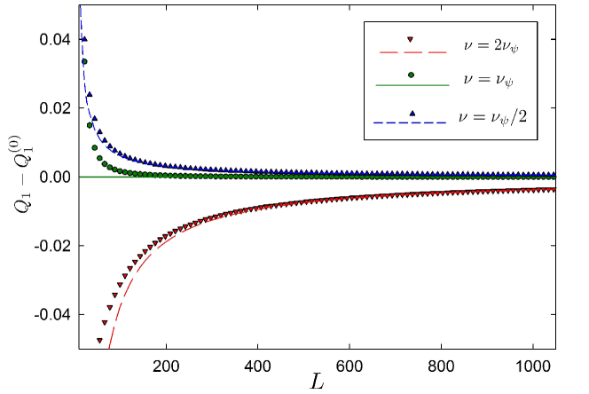
Figure 4.5: Plot of the difference $Q_{1}-Q_{1}^{(0)}$ as a function of the system size $L$. Specifically, we present the plots for $\nu=\pi^{2}$, $\nu=\nu_{\psi}=2\pi^{2}$ and $\nu=4\pi^{2}$. For each of these values, there are two curves: the theoretical curve $Q_{1}^{(1)}/L$ (lines) and the numerical estimate of $Q_{1}$ (symbols). See the legend for details. The finite-size correction is especially small for $\nu=\nu_{\psi}$.

In figure 4.5, we check the above expansion for the zeros of the function $g(q)$. Specifically, we do so for the first zero $q_{1}$: the numerical estimation of $q_{1}$ is compared with the expansion in (4.85) and (4.86) by plotting $Q_{1}-Q_{1}^{(0)}$ as a function of the system size $L$. It is observed that this difference tends to zero as the system size increases, for all the considered values of $\nu$. The finite size correction is especially small for $\nu=\nu_{\psi}=2\pi^{2}$, for which the theoretical correction $Q_{1}^{(1)}$ vanishes. Therefore, finite size corrections are as small as possible for this case, which makes it particularly adequate to investigate the hydrodynamic description, as done in section 4.3 and also in [79, 150, 151].

We want to emphasize that the instability of the HCS is reobtained here as a crossing between the first two nonzero eigenvalues: for $\nu=\nu_{c}=8\pi^{2}$, we have that $Q_{1}^{(0)}=Q_{2}^{(0)}$. On the one hand, for $\nu<\nu_{c}$, the largest nonvanishing eigenvalue is $\lambda_{1}$ ($\lambda_{1}<0$) and dominates the long-time dynamics of the system: the energy $C_{0}$ and all the correlations $C_{k}$ decay with $\exp[\lambda_{1}\omega(1+\alpha)\tau]=\exp(\nu_{\text{\tiny HCS}}^{r}t)$, see below. On the other hand, for $\nu>\nu_{c}$, the dominant term is the one corresponding to $Q_{2}\simeq 2\pi$ and the long time behavior of the system becomes independent of $\nu$.

The large system size limit of the eigenvalues is then

$$\lambda_{n}=-\frac{{Q_{n}^{(0)}}^{2}}{L^{2}}\left[1+L^{-1}\frac{2Q_{n}^{(1)}}{Q_{n}^{(0)}}+\mathcal{O}(L^{-2})\right].$$ (4.87)

Moreover, the exponent in (4.81) controlling the time dependence of the contribution for each mode is

$$\lambda_{n}(1+\alpha)\omega\tau\sim-2{Q_{n}^{(0)}}^{2}\left[1+L^{-1}\frac{2Q_{n}^{(1)}}{Q_{n}^{(0)}}+\mathcal{O}(L^{-2})\right]t,$$ (4.88)

which shows the relevance of the hydrodynamic scale $t$, defined in (4.9), in the large system size limit.

4.5.2 Long time limit

Equation (4.81) gives the general time evolution for the velocity correlations. Here, we show that these correlations tend to their HCS values in the long time limit, provided that $\nu<\nu_{c}$, that is, we are below the instability.

Let us consider the scaled correlations $\tilde{C}_{k}$

$$\tilde{C}_{k}(\tau)=\frac{C_{k}(\tau)}{C_{0}(\tau)}=\frac{c_{k}(\tau)}{\sqrt{2}c_{0}(\tau)},$$ (4.89)

that is, we scale the correlations with the energy $C_{0}\neq 0$. For long enough times, the only relevant contribution to (4.81) stems from the maximum (minimum in absolute value) eigenvalue $\lambda_{1}$. Thus, the time dependence for all the correlations $C_{k}$ (or $c_{k}$) are the same and, consequently, the quotient in (4.89) becomes time-independent for long enough times. Making use of (4.80) and (4.81),

$$\tilde{C}_{k}=\frac{\phi^{(1)}_{k}}{\sqrt{2}\phi^{(1)}_{0}}=-\sin\left(\frac{q_{1}}{2}\right)\csc\left(\frac{L-1}{2}q_{1}\right)\cos\left[\left(\frac{L}{2}-k\right)q_{1}\right],$$ (4.90)

which is nothing but the discrete version of the continuum solution obtained in [155, 151].

We can also derive the rate at which the energy and all the correlations are decaying in the long time limit. Particularizing (4.88) for $n=1$, we have that

$$\lambda_{1}(1+\alpha)\omega\tau\sim-\nu t\left[1-L^{-1}\psi_{\text{\tiny HCS}}+\mathcal{O}(L^{-2})\right]=-\nu_{\text{\tiny HCS}}^{r}t,$$ (4.91)

where $\nu_{\text{\tiny HCS}}^{r}$ is the “renormalized” by fluctuations cooling rate introduced in [155, 151], by applying a multiple scale analysis to find finite size corrections to the hydrodynamic description. Thus, the energy is given by

$$C_{0}(t)=T(t=0)\exp(-\nu_{\text{\tiny HCS}}^{r}t)$$ (4.92)

and the correlations $C_{k}$, with $k>0$, follow from (4.90).

Chapter 5 Global stability, derivation of the $H$-theorem

Here, we aim at investigating the global stability and the possibly associated $H$-theorem for a generalization of the model introduced in the previous chapter. At difference with the approach in [97, 98], our analysis is not restricted to spatially homogeneous situations: we consider the whole space and velocity dependence of the one-particle probability distribution function. More specifically, a general energy injection mechanism is introduced, in which the system may be driven through both the boundaries and the bulk.

We show that, under quite general conditions, the steady state is globally stable. Independently of the initial preparation, the system always ends up in the steady state. Interestingly, it is not necessary to have an $H$-theorem to prove this: it suffices to show that $H$ is decreasing in the long-time limit, not for all times. In this regard, we find a situation that is similar to the proof of the tendency towards the equilibrium curve in systems whose dynamics is governed by master equations with time-dependent transition rates [166, 167, 168, 169, 170, 171, 172].

Our proof of global stability also makes it possible to show the inadequacy of Boltzmann’s $H_{B}$, defined in (1.16), as a candidate for a Lyapunov functional in inelastic systems. Not only is this done for the simplified models considered throughout this thesis, but for a general collision term that does not conserve energy in collisions. Therefore, this result also applies to the inelastic Boltzmann or Enskog equations, employed for granular fluids. Specifically, the main idea is the possibility of reversing the sign of $dH_{B}/dt$ by a suitable choice of the initial PDF. Thus, $dH_{B}/dt$ cannot have a definite sign. In this sense, our result can be understood as a generalization of that in [101], within the first Sonine approximation of the inelastic Boltzmann equation, to an arbitrary collision kernel with nonconservative interactions.

Having proved global stability by showing that $H$ is a nonincreasing functional for long times, a natural question arises. Is $H$ a Lyapunov function, that is, a nonincreasing functional for all times? There does not seem to be a unique proof, valid for any driving mechanism, even within the framework of our simplified model. Notwithstanding, we have been able to derive a specific proof for a quite general driving mechanism, which includes as limiting cases both the sheared system and the uniformly heated system [57, 173, 174, 162, 175, 176, 112, 113, 177]. Our proof is based on a suitable expansion of the one-particle PDF in Hermite polynomials, which is a generalization of the customary Sonine expansion of kinetic theory.

The plan of this chapter is detailed below. We introduce the aforementioned generalized model and study its stationary states in section 5.1. The main difference is the consideration of a thermostat, allowing an energy input not only through boundaries, but also through the bulk. Section 5.2 is devoted to the proof of the global stability of the nonequilibrium steady states for this general energy injection mechanism. The inadequacy of Boltzmann’s $H_{B}$ as a Lyapunov functional for inelastic systems is discussed in section 5.3. Finally, in section 5.4, we consider some concrete physical situations in our model, which include the sheared and the uniformly heated systems. Therein, we prove that the functional $H$, which is used in the proof of global stability, is a monotonically decreasing Lyapunov functional. In this way, we prove an $H$-theorem for our system with nonconservative interactions.

5.1 Basics of the model

5.1.1 The stochastic forcing

As introduced above, in this chapter we use a generalization of the model presented in the previous chapter. In addition to collisions (4.1), the system is heated by a stochastic force that is modeled by a white noise that affects all sites, the so-called stochastic thermostat [57, 173, 174, 162, 175, 176, 112, 113, 177, 114, 115, 116]. Specifically, for a short time interval, the change of the velocity due to the heating is given by

$$\left.\Delta v_{i}(\tau)\right|_{\text{noise}} \equiv\left.v_{i}(\tau+\Delta\tau)-v_{i}(\tau)\right|_{\text{noise}}$$

$$=\left(\xi_{i}(\tau)-\frac{1}{N}\sum_{j=1}^{N}\xi_{j}(\tau)\right)\Delta\tau,$$ (5.1)

where $\xi_{i}(t)$ are Gaussian white noises, verifying

$$\langle\xi_{i}(\tau)\rangle_{\text{noise}}=0,\quad\langle\xi_{i}(\tau)\xi_{j}(\tau^{\prime})\rangle_{\text{noise}}=\chi\delta_{ij}\delta(\tau-\tau^{\prime}),$$ (5.2)

for $i,j=1,\ldots,N$. Above, $\chi$ is the amplitude of the noise, and $\langle\cdots\rangle_{\text{noise}}$ denotes the average over the different realizations of the noise. Note that this version of the stochastic thermostat conserves total momentum, a necessary condition to have a steady state [176, 177, 165].

We turn our attention to the probability density of finding the system in state $\bm{v}$ at time $\tau$, $P_{N}(\bm{v},\tau)$ . The stochastic process $\bm{v}(\tau)$ is Markovian and the equation governing the time evolution of $P_{N}(\bm{v},\tau)$ has two contributions. First, we have the master equation contribution stemming from collisions, as given by (4.7) with $\beta=0$,

$$\left.\partial_{\tau}P_{N}(\bm{v},\tau)\right|_{\text{coll}}=\omega\sum_{l=1}^{N}\left[\frac{P_{N}(\hat{b}_{l}^{-1}\bm{v},\tau)}{\alpha}-P_{N}(\bm{v},\tau)\right].$$ (5.3)

Second, there is a Fokker-Planck contribution stemming from the stochastic forcing [97, 98]

$$\left.\partial_{\tau}P_{N}(\bm{v},\tau)\right|_{\text{noise}}=\frac{\chi}{2}\sum_{i,j=1}^{N}\left(\delta_{ij}-\frac{1}{N}\right)\frac{\partial^{2}}{\partial v_{i}\partial v_{j}}P_{N}(\bm{v},\tau).$$ (5.4)

The time evolution of $P_{N}(\bm{v},\tau)$ is obtained by combining (5.3) and (5.4), that is,

$$\partial_{\tau}P_{N}(\bm{v},\tau)=\left.\partial_{\tau}P_{N}(\bm{v},\tau)\right|_{\text{coll}}+\left.\partial_{\tau}P_{N}(\bm{v},\tau)\right|_{\text{noise}}.$$ (5.5)

We can derive the evolution equation of the one-particle distribution function in the “hydrodynamic” continuous space and time variables $x=(l-1)/L$ and $t=\omega\tau/L^{2}$. As in the previous chapter, we assume molecular chaos to get a closed evolution equation for $P_{1}(v;x,t)$

$$\partial_{t}P_{1}(v;x,t)=\partial_{x}^{2}P_{1}(v;x,t)+\frac{\nu}{2}\partial_{v}\left\{[v-u(x,t)]P_{1}(v;x,t)\right\}+\frac{\xi}{2}\partial_{v}^{2}P_{1}(v;x,t),$$ (5.6)

where we recall that $u(x,t)$ is the local average velocity and $\nu=(1-\alpha^{2})L^{2}$ is the macroscopic dissipation coefficient. The macroscopic noise strength $\xi$ is given by

$$\xi=\frac{\chi L^{2}}{\omega}.$$ (5.7)

This shows that the microscopic noise strength $\chi$ must scale as $L^{-2}$ in order to have a finite contribution in the continuum limit. Of course, for $\xi=0$, we recover the kinetic equation for the case in which there is no stochastic forcing, see (4.30).

From the kinetic equation for $P_{1}(v;x,t)$, one can derive the evolution equations for the profiles $u(x,t)$ and $T(x,t)$,

$$\partial_{t}u =\partial_{xx}u,$$ (5.8a)

$$\partial_{t}T =-\nu T+\partial_{x}^{2}T+2\left(\partial_{x}u\right)^{2}+\xi.$$ (5.8b)

Note that the only difference with (4.16) is an extra term $\xi$ in the temperature equation, corresponding to the uniform heating.

5.1.2 Nonequilibrium steady states

We are interested in the driven cases. Therein, energy loss in collisions is eventually balanced (in average) by the energy input, and in the long time limit the system reaches a steady state. These nonequilibrium steady states (NESS) are described by the corresponding stationary solutions $P^{(\text{s})}_{1}(v;x)$ of the kinetic equation, which verify

$$0=\partial_{x}^{2}P^{(\text{s})}_{1}(v;x)+\frac{\nu}{2}\partial_{v}\left\{[v-u_{\text{s}}(x)]P^{(\text{s})}_{1}(v;x)\right\}+\frac{\xi}{2}\partial_{v}^{2}P^{(\text{s})}_{1}(v;x),$$ (5.9)

where $u_{\text{s}}(x)$ is the stationary average velocity profile. In this chapter, to be concrete, we consider two cases: a system that is (a) sheared and (b) uniformly heated.

First, let us consider the sheared system that we analyzed in section 4.3.2, for which there is no stochastic forcing, $\xi=0$. The stationary values for the average velocity and temperature in the USF are those in (4.41), whereas the stationary distribution is given by (4.45), and thus we do not repeat them here.

Second, we address the uniformly heated system, $\xi\neq 0$, but without any shear, $a=0$ in 4.40 and 4.43. In other words, we have the usual periodic boundary conditions. In the steady state, the system is homogeneous: there is no average velocity and the temperature is uniform,

$$u_{\text{s}}(x)=0,\quad T_{\text{s}}=\frac{\xi}{\nu}.$$ (5.10)

The corresponding stationary PDF is also Gaussian,

$$P^{(\text{s})}_{1}(v;\cancel{x})=\left(2\pi T_{\text{s}}\right)^{-1/2}\exp\left[-\frac{v^{2}}{2T_{\text{s}}}\right].$$ (5.11)

With this “stochastic thermostat” forcing, the system remains homogeneous for all times if it is initially so, as is also the case of a inelastic gas of hard particles described by the inelastic Boltzmann equation [57].

5.2 Proof of global stability

In this section, we analyze the global stability of the nonequilibrium stationary solutions of the kinetic equation (5.6). We do so for quite a general class of boundary conditions. Following the discussion in section 1.2.2, we define the $H$-functional as

$$H[P_{1}]=\int\!\!dx\,dvP_{1}(v;x,t)\ln\!\left[\frac{P_{1}(v;x,t)}{P^{(\text{s})}_{1}(v;x)}\right],$$ (5.12)

note the analogy with (1.19).

Let us consider the time evolution of $H[P_{1}]$. It is directly obtained that

$$\frac{dH}{dt}=\int\!\!dx\,dv\,\partial_{t}{\left[P_{1}\ln\left(\frac{P_{1}}{P^{(\text{s})}_{1}}\right)\right]}=\int\!\!dx\,dv\,\left(\mathcal{L}P_{1}\right)\,\ln\left(\frac{P_{1}}{P^{(\text{s})}_{1}}\right),$$ (5.13)

where $\mathcal{L}$ stands for the nonlinear evolution operator on the rhs of the kinetic equation (5.6), that is, $\partial_{t}{P_{1}}=\mathcal{L}P_{1}$. Now we make use of the following property: if we define $\Delta P_{1}=P_{1}-P^{(\text{s})}_{1}$ to be the deviation of the PDF from the steady state, the linear terms in the deviation vanish, since both factors in the integrand of (5.13) are equal to zero for $P_{1}=P^{(\text{s})}_{1}$. This is a desirable property: were it not true, the sign of $dH/dt$ could be reversed for initial conditions close enough to the steady state by simply reversing the initial value of $\Delta P_{1}$. Thus, the existence of an $H$-theorem would be utterly impossible, see also next section.

Then, we can write

$$\frac{dH}{dt}=\int\!\!dx\,dv\,\left(\mathcal{L}P_{1}\right)\,\ln\left(\frac{P_{1}}{P^{(\text{s})}_{1}}\right)-\int\!\!dx\,dv\,\left(\mathcal{L}P^{(\text{s})}_{1}\right)\,\frac{P_{1}-P^{(\text{s})}_{1}}{P^{(\text{s})}_{1}}.$$ (5.14)

Now, the idea is to split the operator $\mathcal{L}$ into the three contributions on the rhs of (5.6): first, the diffusive one; second, the one proportional to $\nu$, which is intrinsically dissipative; and third, the one proportional to the noise strength $\xi$: $\mathcal{L}_{\text{diff}}$, $\mathcal{L}_{\text{inel}}$ and $\mathcal{L}_{\text{noise}}$, respectively. Accordingly, we have that the time derivative of $H$ has three contributions,

$$\frac{dH}{dt}=\left.\frac{dH}{dt}\right|_{\text{diff}}+\left.\frac{dH}{dt}\right|_{\text{inel}}+\left.\frac{dH}{dt}\right|_{\text{noise}},$$ (5.15)

obtained by inserting into (5.14) the relevant part of the evolution operator $\mathcal{L}$. Note that, although $\mathcal{L}P^{(\text{s})}_{1}=0$, in general $\mathcal{L}_{\text{diff}}P^{(\text{s})}_{1}\neq 0$, $\mathcal{L}_{\text{inel}}P^{(\text{s})}_{1}\neq 0$ and $\mathcal{L}_{\text{noise}}P^{(\text{s})}_{1}\neq 0$.

After some tedious but easy algebra, collected in Appendix E, the following expressions are derived. Firstly, for the diffusive term,

$$\left.\frac{dH}{dt}\right|_{\text{diff}}=-\int\!\!dx\,dv\,P_{1}\left(\partial_{x}{\ln P_{1}}-\partial_{x}{\ln P^{(\text{s})}_{1}}\right)^{2}\leq 0.$$ (5.16)

Secondly, for the inelastic term, proportional to $\nu$,

$$\left.\frac{dH}{dt}\right|_{\text{inel}}=-\frac{\nu}{2}\int\!\!dx\left(u-u_{\text{s}}\right)\int\!\!dvP_{1}\,\partial_{v}{\ln P^{(\text{s})}_{1}}.$$ (5.17)

Finally, the noise term, proportional to $\xi$, reads

$$\left.\frac{dH}{dt}\right|_{\text{noise}}=-\frac{\xi}{2}\int\!\!dx\,dv\,P_{1}\left(\partial_{v}{\ln P_{1}}-\partial_{v}{\ln P^{(\text{s})}_{1}}\right)^{2}\leq 0.$$ (5.18)

These results, and the following throughout this section, are valid for a quite general set of boundary conditions, leading to the cancellation of all the boundary terms arising after integrating by parts, as detailed in Appendix E. This set includes but is not limited to the Lees-Edwards and periodic boundary conditions corresponding to the sheared and uniformly heated situations, respectively. For instance, they also apply to the Couette state, in which the system is driven by keeping its two edges at two (in general, different) fixed temperatures $T_{L}$ and $T_{R}$.

The inelastic term $dH/dt|_{\text{inel}}$ in (5.17) does not have a definite sign in general. Therefore, it is the inelastic term that prevents us from proving $H$ to be a nonincreasing function of time. It must be stressed that the diffusive, inelastic and noise contributions to $dH/dt$ in (5.16)-(5.17) come exclusively from the diffusive, noise and inelastic contributions in the kinetic equation, respectively, only once the linear terms have been subtracted as is done in (5.14), see Appendix E for details.

Despite the above discussion, global stability of the steady state can be established without proving an $H$-theorem. The key point is the following: the long time limit of $dH/dt$ is nonpositive and thus $H$ has a finite limit, since it is bounded from below. Therefore, $dH/dt$ tends to zero in the long time limit and it can be shown that this is only the case if $P_{1}(v;x,\infty)\equiv\lim_{t\to\infty}P_{1}(v;x,t)=P^{(\text{s})}_{1}(v;x)$.

The average velocity $u(x,t)$ satisfies a diffusive equation (5.8a), and thus it irreversibly tends to the steady profile corresponding to the given boundary conditions in the long time limit. Therefore, $u(x,\infty)\equiv\lim_{t\to\infty}u(x,t)=u_{\text{s}}(x)$ and taking into account (5.17),

$$\lim_{t\to\infty}\left.\frac{dH}{dt}\right|_{\text{inel}}=0\Rightarrow\lim_{t\to\infty}\frac{dH}{dt}\leq 0.$$ (5.19)

Since $H[P_{1}]$ is bounded from below, the only possibility is

$$\lim_{t\to\infty}\frac{dH}{dt}=0,$$ (5.20)

and all the contributions to $dH/dt$ in (5.16)-(5.18) vanish in the long time limit. The vanishing of (5.16) imposes that

$$P_{1}(v;x,\infty)=P^{(\text{s})}_{1}(v;x)\phi(v;t),$$ (5.21)

where $\phi(v;t)$ is an arbitrary function of $v$ and $t$. For $\xi\neq 0$, (5.18) implies that $\phi(v;t)$ must be a function depending only of time, independent of $v$, and normalization yields $\phi(v;t)=1$. For $\xi=0$, (5.18) identically vanishes but it can be also shown that $\phi(v;t)=1$, see appendix F for details. Thus, for arbitrary $\xi$, including $\xi=0$, we have that

$$P_{1}(v;x,\infty)=P^{(\text{s})}_{1}(v;x).$$ (5.22)

The steady distribution $P^{(\text{s})}_{1}(v;x)$ is globally stable. Each time evolution $P_{1}(v;x,t)$, corresponding to a given initial condition, tends to $P^{(\text{s})}_{1}(v;x)$ in the long time limit.

5.3 Why cannot Boltzmann’s $H_{B}$ be the “good” Lyapunov functional?

Here we prove that Boltzmann’s $H_{B}[P_{1}]$, given by (1.16), cannot be used to build a Lyapunov functional for intrinsically dissipative systems, in agreement with the numerical results by Marconi et al. [97]. Not only does our proof hold for the simplified models considered here, but for a general kinetic equation in which energy is not conserved in collisions, such as the inelastic Boltzmann or Enskog equations. To keep the notation simple, we still write $\partial_{t}{P_{1}}=\mathcal{L}P_{1}$, but now $\mathcal{L}$ stands for the evolution operator in the considered kinetic description, which is nonlinear in general.

First, we restrict ourselves to homogeneous situations and thus drop the integral over $x$,

$$H_{B}[P_{1}]= \int\!\!dvP_{1}\ln P_{1},$$ (5.23a)

$$\frac{dH_{B}}{dt}= \int\!\!dv\,\partial_{t}{P_{1}}\ln P_{1}=\int\!\!dv\,\left(\mathcal{L}P_{1}\right)\,\ln P_{1},$$ (5.23b)

Also, we consider a system that is initially close to the steady state, such that we can expand everything in powers of $\Delta P_{1}=P_{1}-P^{(\text{s})}_{1}$. Then,

$$\mathcal{L}P_{1}\equiv\mathcal{L}(P^{(\text{s})}_{1}+\Delta P_{1})=\cancelto{0}{\mathcal{L}P^{(\text{s})}_{1}}+\mathcal{L}_{\text{lin}}\Delta P_{1}+O(\Delta P_{1})^{2},$$ (5.24)

in which $\mathcal{L}_{\text{lin}}$ is the linearized evolution operator. Neglecting $O(\Delta P_{1})^{2}$ terms, the linear approximation arises,

$$\left.\frac{dH_{B}}{dt}\right|_{\text{lin}}=\int\!\!dv\,(\mathcal{L}_{\text{lin}}\Delta P_{1})\,\ln P^{(\text{s})}_{1}=\left.\frac{d}{dt}\langle\ln P^{(\text{s})}_{1}\rangle\right|_{\text{lin}}.$$ (5.25)

On the one hand, the linear contribution vanishes in the elastic case: $\ln P^{(\text{s})}_{1}$ is a sum of constants of motion, which are unchanged by the linearized kinetic operator. Then, $H_{B}$ can be a candidate for a Lyapunov functional. On the other hand, only mass and linear momentum are conserved for nonconservative interactions. Thus, no longer is $\ln P^{(\text{s})}_{1}$ a sum of conserved quantities, and

$$\left.\frac{dH_{B}}{dt}\right|_{\text{lin}}\neq 0.$$ (5.26)

Therefore, by changing the initial sign of $\Delta P_{1}=P_{1}-P^{(\text{s})}_{1}$, which can always be done, the initial sign of $dH_{B}/dt$ is reversed and $H_{B}$ cannot be a Lyapunov functional.

In figure. 5.1, we show the evolution of $H_{B}$ in our kinetic model. We consider a uniformly heated system, so that the system remain homogeneous for all times, as described in section 5.1.2. Two different initial conditions are considered, corresponding to Gaussian distributions with zero average velocity but nonsteady values of the temperature, specifically $1.1\,T_{\text{s}}$ and $0.9\,T_{\text{s}}$. We can see how, in agreement with our discussion, not only is one of the functionals increasing, but also it can be obtained as the mirror image of the decreasing one through the stationary value. Simulations, as have been repeatedly stated throughout the thesis, are performed following the recipe given in Appendix C.

Taking into account the specific (Gaussian) shape of the steady PDF for the uniformly heated system, as given by (5.11), the time derivative of $H_{B}$ in (5.25) reduces to

$$\frac{dH_{B}}{dt}=-\frac{1}{2T_{\text{s}}}\frac{d\langle v^{2}\rangle}{dt}.$$ (5.27)

Since the plots in figure 5.1 correspond to evolutions of the system for which $u(x,t)\equiv 0$ for all times, therein $\langle v^{2}\rangle=T$ and, consistently, the $H_{B}$-curve corresponding to an initial value of the temperature that is higher (lower) than the steady one monotonically increases (decreases).

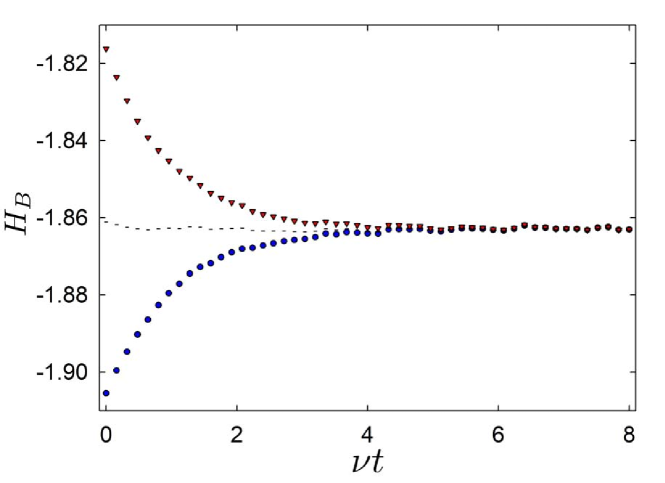
Figure 5.1: Time evolution of the functional $H_{B}$. Specifically, we consider two different initial conditions in a uniformly heated system. Both simulations start from a Gaussian distribution with a homogeneous temperature, which slightly differs from the stationary one: (i) $T(t=0)=1.1\,T_{\text{s}}$ (blue circles) and (ii) $T(t=0)=0.9\,T_{\text{s}}$ (red triangles). Both functionals are symmetric with respect to its stationary value in agreement with the prediction of the linear approximation. Consistently, the mean value of both curves (dashed line) remains approximately constant throughout. We have considered a system with parameters $\nu=20$ and $\xi=50$, size $N=330$, and averaged over $3000$ trajectories.

The above picture is consistent with the situation found in [101], in which the uniformly heated granular gas described by the inelastic Boltzmann equation was investigated within the first Sonine approximation. Therein, the entropy production was shown to have linear terms in the deviations of the temperature and the excess kurtosis. Also, our result is consistent with the numerical results in [97] for several collision models. In particular, observe the similarity with the situation reported in panels A and B of figure 1.9 of the introduction to this thesis. Note that our argument also proves why $H_{B}$ cannot be nonincreasing for an elastic system immersed in a heat bath at a temperature different from the initial temperature of the gas, as also observed in [97]. Although $\ln P^{(\text{s})}_{1}$ is conserved in collisions, the evolution operator includes a term coming from the interaction with the bath that does not conserve the kinetic energy, and again $dH/dt|_{\text{lin}}\neq 0$, making it impossible for $H_{B}$ to be a “good” Lyapunov functional.

In spatially inhomogeneous situations, the main difference is the additional integral over space, both in $H_{B}$ and, consequently, $dH_{B}/dt$. There is no reason to expect this integral over space to make $dH/dt|_{\text{lin}}$ vanish, since one still has that

$$\left.\frac{dH_{B}}{dt}\right|_{\text{lin}}=\left.\frac{d}{dt}\langle\ln P^{(\text{s})}_{1}\rangle\right|_{\text{lin}},$$ (5.28)

and, in general, $\ln P^{(\text{s})}_{1}$ is not a sum of constants of motion. In fact, again the sign of $\left.dH_{B}/dt\right|_{\text{lin}}$ is reversed when $\Delta P_{1}\to-\Delta P_{1}$, similarly to the homogeneous case. In figure 5.2, we have numerically checked this prediction for the sheared system, with the resulting evolution of $H_{B}$ being completely similar to that for the uniformly heated case in figure 5.1.

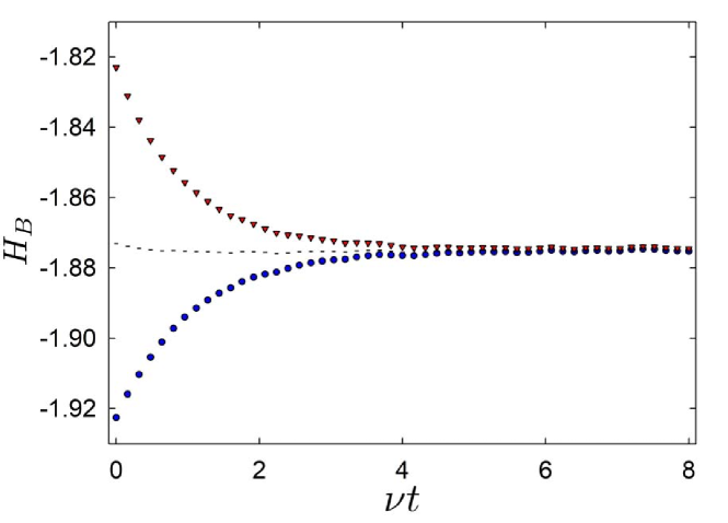
Figure 5.2: Time evolution of the functional $H_{B}$. Analogously to figure 5.1, we consider two different initial conditions, but now for a sheared system. Both simulations start from a Gaussian distribution with the stationary average velocity profile but a homogeneous temperature, which slightly differs from the stationary one: (i) $T(t=0)=1.1\,T_{\text{s}}$ (blue circles) and (ii) $T(t=0)=0.9\,T_{\text{s}}$ (red triangles). We have considered a system with parameters $\nu=20$ and $a=5$, size $N=660$, and averaged over $6000$ trajectories.

5.4 $H$-theorem for some specific NESS

Here we prove that the functional $H[f]$ is monotonically decreasing for all times in some specific physical situations. Our proof applies both to the sheared and the uniformly heated systems described in section 5.1.2. To be as general as possible, we consider a system that is both heated and sheared: $a\neq 0$ and $\xi\neq 0$. In this situation, the boundary conditions for the PDF are given by (4.43), which lead to the Lees-Edwards boundary conditions (4.40) for the averages $u(x,t)$ and $T(x,t)$.

The steady solution of the hydrodynamic equations is

$$u_{\text{s}}(x)=a\left(x-\frac{1}{2}\right),\qquad T_{\text{s}}=\frac{2a^{2}+\xi}{\nu}.$$ (5.29)

On the one hand, the average velocity has a linear profile, similarly to the situation in the USF state. On the other hand, the temperature remains homogeneous but its steady value has two contributions, one coming from the shear and the other from the stochastic thermostat. The viscous heating $2(\partial_{x}{u})^{2}$ and uniform heating $\xi$ terms cancel the cooling term $-\nu T$ for all $x$. The stationary solution of the kinetic equation is the Gaussian distribution (4.45) corresponding to the hydrodynamic fields in (5.29). Of course, the USF state and NESS of the uniformly heated system in section 5.1.2 can be easily recovered as particular cases of (4.45): for $(a\neq 0,\xi=0)$ and $(a=0,\xi>0$), respectively.

Then, we turn now to the question of the existence of an $H$-theorem, that is, the existence of a nonequilibrium entropy ensuring the monotonic approach of the one-particle PDF to the steady state. Our starting point is the following expansion of the one-particle PDF in Hermite polynomials,

$$P_{1}(v;x,t)=\frac{1}{\sqrt{2\pi T(x,t)}}\exp\left\{-\frac{[v-u(x,t)]^{2}}{2T(x,t)}\right\}\left\{1+\sum_{n=3}^{\infty}\gamma_{n}(x,t)\,H_{n}\!\!\left[\frac{v-u(x,t)}{\sqrt{T(x,t)}}\right]\right\},$$ (5.30)

which is known as the Gram-Charlier series [178, 179, 180, 181]. Therein, $u(x,t)$ and $T(x,t)$ are the (exact) average velocity and temperature stemming from the hydrodynamic equations for the considered distribution. Note that the argument of the Hermite polynomials is the scaled velocity $c$ defined in (4.32). The above expansion is suggested by the Gaussian shape of the stationary PDF in (4.45). Making use of the definition (4.32) of the scaled one-particle distribution function $\varphi(c;x,t)$ and the orthogonality relation of the Hermite polynomials [182], it is readily obtained that

$$\varphi(c;x,t)=\frac{1}{\sqrt{2\pi}}\exp\left(-\frac{c^{2}}{2}\right)\left[1+\sum_{n=3}^{\infty}\gamma_{n}(x,t)\,H_{n}(c)\right],$$ (5.31)

with

$$\gamma_{n}(x,t)=\frac{1}{n!}\int\!\!dc\,H_{n}(c)\varphi(c;x,t).$$ (5.32)

Also, we could have written $\gamma_{n}$ as a combination of moments of the distribution.

Some comments on the Gram-Charlier expansion are pertinent. First, note that $n\geq 3$ in the sum: $\gamma_{1}=\gamma_{2}=0$ because the zero-th order Gaussian contribution exactly gives the first two moments $\langle v\rangle(x,t)=u(x,t)$ and $\langle v^{2}\rangle(x,t)=u^{2}(x,t)+T(x,t)$. Second, if $P_{1}(v;x,t)$ were symmetric with respect to $v=u$, that is, $\langle(v-u)^{2n+1}\rangle=0$ for all $n\in\mathbb{N}$, only even values of $n$ would be present in the sum and one recovers the usual expansion in Sonine-Laguerre polynomials of kinetic theory. Finally, it is worth stressing that the series (5.30) converges for functions such that the tails of $\varphi(c;x,t)$ approach zero faster than $e^{-c^{2}/4}$ for $c\to\pm\infty$ [183, 184, 181].

Now we substitute the Gaussian stationary solution (4.45) and the Gram-Charlier series (5.30) into the three contributions to $dH/dt$, given by (5.16), (5.17) and (5.18). For the inelastic term, it is readily obtained that

$$\left.\frac{dH}{dt}\right|_{\text{inel}}=\frac{\nu}{2T_{\text{s}}}\int\!\!dx\left(u-u_{\text{s}}\right)^{2}.$$ (5.33)

For the diffusive and noise terms, the key ideas are a change of the integration variable from $v$ to $c=(v-u)/\sqrt{T}$ and the use of the recursion relations and the orthogonality property of the Hermite polynomials [182]. Working along these guidelines, we arrive at

$$\left.\frac{dH}{dt}\right|_{\text{diff}}= -\int\!\!dx\,T\left(\frac{u^{\prime}}{T}-\frac{u_{\text{s}}^{\prime}}{T_{\text{s}}}\right)^{2}-\frac{u_{\text{s}}^{\prime 2}}{T_{\text{s}}^{2}}\int\!\!dx\left(u-u_{\text{s}}\right)^{2}$$

$$-\frac{1}{\sqrt{2\pi}}\int\!\!dx\,dc\,\frac{e^{-c^{2}/2}}{1+\sum_{n=3}^{\infty}\gamma_{n}H_{n}(c)}\left\{\frac{T^{\prime}}{2T}H_{2}(c)+\sum_{n=3}^{\infty}\gamma_{n}^{\prime}H_{n}(c)\right.$$

$$\qquad\qquad\left.-\sum_{n=3}^{\infty}\frac{\gamma_{n}u^{\prime}}{\sqrt{T}}nH_{n-1}(c)+\sum_{n=3}^{\infty}\frac{\gamma_{n}T^{\prime}}{2T}\left[H_{n+2}(c)+nH_{n}(c)\right]\right\}^{2},$$ (5.34)

$$\left.\frac{dH}{dt}\right|_{\text{noise}}= -\frac{\xi}{2}\int\!\!dx\,T\left(\frac{1}{T}-\frac{1}{T_{\text{s}}}\right)^{2}-\frac{\xi}{2T_{\text{s}}^{2}}\int\!\!dx\left(u-u_{\text{s}}\right)^{2}$$

$$-\frac{\xi}{2\sqrt{2\pi}}\int\!\!dx\,dc\,\frac{e^{-c^{2}/2}}{1+\sum_{n=3}^{\infty}\gamma_{n}H_{n}(c)}\frac{1}{T}\left[\sum_{n=3}^{\infty}\gamma_{n}nH_{n-1}(c)\right]^{2},$$ (5.35)

where the prime stands for spatial derivative. In (5.33), (5.34) and (5.35) there are several terms multiplying $\int\!\!dx\left(u-u_{\text{s}}\right)^{2}$: they cancel out when we take into account the equation for the (spatially homogeneous) stationary temperature. Therefore, the sum of the remaining terms leads right to

$$\frac{dH}{dt}=A(t)+B(t),\quad\text{with both }A(t),B(t)\leq 0,$$ (5.36)

being

$$A(t)=-\int\!\!dx\,T\left[\left(\frac{u^{\prime}}{T}-\frac{u_{\text{s}}^{\prime}}{T_{\text{s}}}\right)^{2}+\frac{\xi}{2}\left(\frac{1}{T}-\frac{1}{T_{\text{s}}}\right)^{2}\right],$$ (5.37)

and $B(t)$ the sum of the second and third line in (5.34) with the second line in (5.35), that is,

$$B(t)= -\frac{1}{\sqrt{2\pi}}\int\!\!dx\,dc\,\frac{e^{-c^{2}/2}}{1+\sum_{n=3}^{\infty}\gamma_{n}H_{n}(c)}\left\{\frac{\xi}{2T}\left[\sum_{n=3}^{\infty}\gamma_{n}nH_{n-1}(c)\right]^{2}+\left[\frac{T^{\prime}}{2T}H_{2}(c)\right.\right.$$

$$\qquad+\sum_{n=3}^{\infty}\gamma_{n}^{\prime}H_{n}(c)-\left.\left.\sum_{n=3}^{\infty}\frac{\gamma_{n}u^{\prime}}{\sqrt{T}}nH_{n-1}(c)+\sum_{n=3}^{\infty}\frac{\gamma_{n}T^{\prime}}{2T}\left\{H_{n+2}(c)+nH_{n}(c)\right\}\right]^{2}\right\},$$ (5.38)

In conclusion, $dH/dt\leq 0$ for all times and we have shown that the $H$-theorem holds for the sheared and heated system. Rigorously, our proof holds for those PDFs such that the above Hermite expansion converges. Note that the proof remains valid for the approach to any NESS, whose PDF is a Gaussian with a homogeneous temperature, independently of the corresponding boundary conditions. In section 5.2, we have already demonstrated that $dH/dt$ only vanishes for $P_{1}(v;x,\infty)=P^{(\text{s})}_{1}(v;x)$, but the same result can be rederived here in a different way. By imposing that both $A(t)$ and $B(t)$ vanish in the long time limit and making use of the hydrodynamic equations for the averages, it can be shown that $u(x,\infty)=u_{\text{s}}(x)$, $T(x,\infty)=T_{\text{s}}$ and $\gamma_{n}(x,\infty)=0$, $\forall n\geq 3$.

5.4.1 USF state: simulations

Here we consider the sheared system in order to check numerically our theoretical predictions. Throughout this section, we employ the values of the parameters $\nu=20$ and $a=5$. Note that $\xi=0$, since there is no stochastic forcing.

First, in figure 5.3, we show the evolution of the distribution and the $H$-functional from a Gaussian initial condition with the steady velocity profile $u(x,0)=u_{\text{s}}(x)$ but a higher temperature, $T(t=0)=7\,T_{\text{s}}$. In the top panel, we depict the velocity distribution at $x=1/4$ for several times. All of them are Gaussian, which agrees with the theoretical prediction of the kinetic equation: when the initial velocity profile coincides with the steady one and only the temperature is perturbed, an initially Gaussian PDF remains Gaussian for all times. Indeed, we can see in the inset how the excess kurtosis,

$$\kappa=\langle[v-u(x)]^{4}\rangle/\langle[v-u(x)]^{2}\rangle^{2}-3,$$ (5.39)

only fluctuates around zero at the considered position, consistently with the Gaussian shape. In the bottom panel, it is neatly observed that the $H$-functional monotonically decreases in time.

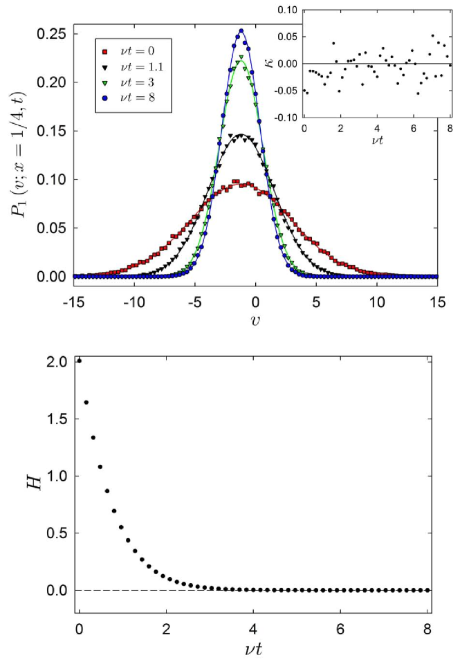
Figure 5.3: Relaxation towards the USF state. The initial distribution is Gaussian, with average velocity in $u_{\text{s}}(x)$ and temperature $T=7\,T_{\text{s}}$. (Top) Velocity distribution function at $x=1/4$. Four different times are shown, as labeled. In the inset, we present the evolution of the excess kurtosis. Solid lines correspond to the (theoretical) Gaussian distributions for the plotted times, except for the longest in which it represents the theoretical steady distribution. (Bottom) Relaxation of the $H$ functional, which is clearly monotonically decreasing to zero. System size is $N=660$, parameters are $\nu=20$ and $a=5$, and curves are averaged over $6000$ runs.

Second, we look into the relaxation to the USF state from another initial preparation, for which the velocity profile $u(x,0)$ is different from the stationary but $T(x,0)=T_{\text{s}}$. The numerical results are shown in figure 5.4, and for the sake of simplicity we use again an initial Gaussian distribution. Specifically, we have that $u(x,0)=u_{\text{s}}(x)+4.4\,\sin(2\pi x)$. Here, the departure from the Gaussian shape is evident, and thus we have not plotted the kurtosis. Consistently with our theoretical prediction, we get again a monotonous relaxation of $H$ towards its null stationary value.

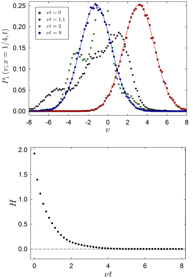
Figure 5.4: The same plots as in figure 5.3, but starting from a different initial condition. Now, the initial PDF is a Gaussian with average velocity $u(x,0)=u_{\text{s}}(x)+4.4\,\sin(2\pi x)$ and temperature $T(t=0)=T_{\text{s}}$. In the top panel, solid lines correspond to the theoretical PDFs for the initial time and the steady state. In the bottom panel, $H$ decreases again monotonically towards its steady value, consistently with our theory.

Finally, we consider situations for which the above presented proof is not rigorously applicable. As stated before, the Gram-Charlier series does not converge when the tails of the distribution decay to zero slower than the square root of the Gaussian. Nevertheless, when all the coefficients $\gamma_{n}$ defined in (5.32) exist and are finite, we still expect the $H$-theorem to hold. We illustrate this situation with an initial exponential distribution; specifically, we consider

$$P_{1}(v;x,0)=\frac{1}{\sqrt{2T(t=0)}}\exp\left[\frac{\sqrt{2}\left|v-u(x,t=0)\right|}{\sqrt{T(t=0)}}\right],$$ (5.40)

with $u(x,t=0)=u_{\text{s}}(x)+4.4\sin(2\pi x)$ and $T(t=0)=0.1\,T_{\text{s}}$. In agreement with our expectation, the $H$-functional also monotonically decreases in figure 5.5.

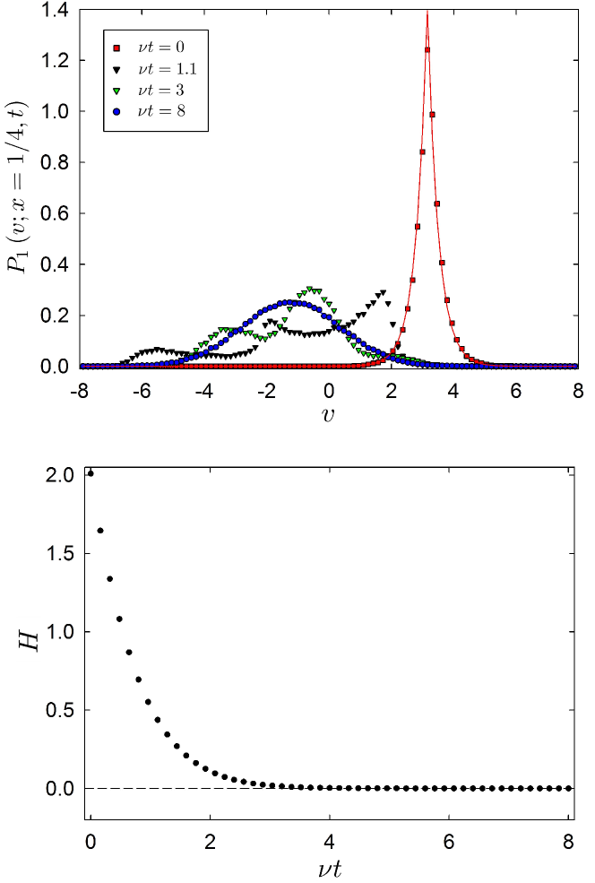
Figure 5.5: The same plots as in figure 5.3, but starting from an initial PDF with a divergent Gram-Charlier series. Specifically, they correspond to an exponential initial distribution with average velocity $u(x,t=0)=u_{\text{s}}(x)+4.4\,\sin(2\pi x)$ and temperature $T(t=0)=0.1\,T_{\text{s}}$.

5.4.2 Numerical results in the uniformly heated system

To conclude, we put forward the results of simulations for the uniformly heated system. Specifically, our simulations have been done for $\nu=20$, $a=0$ (no shear) and $\xi=50$. In order not to be repetitive, we only present the more complex case in figure 5.6: the relaxation towards the steady state from an initial exponential distribution, as given by (5.40). In particular, we consider that $u(x,t=0)=4.4\,\sin(2\pi x)$ and $T(t=0)=0.1\,T_{\text{s}}$. Note that the perturbation from the steady values is the same as in figure 5.5 for the sheared case. Once more, we observe the monotonic relaxation of $H$ towards its stationary value, in neat agreement with our theoretical result, even for a initial distribution for which the Gram-Charlier series does not converge.

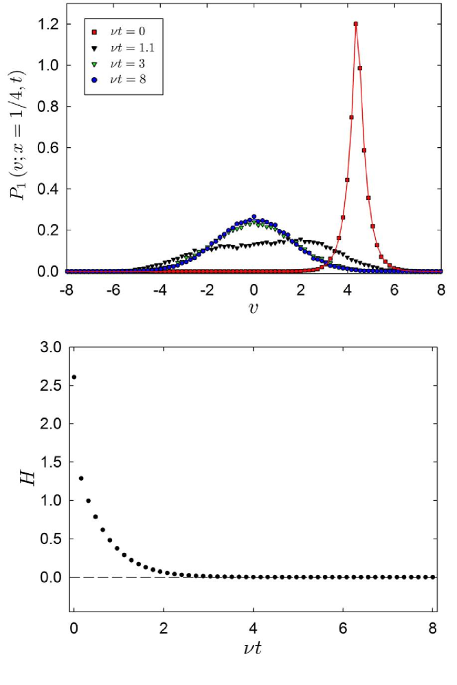
Figure 5.6: Numerical results for the uniformly heated system. Similar to what we did in figure 5.3, we show the time evolution of the PDF (top) and the time evolution of the $H$-functional (bottom). The system is initially prepared with an exponential PDF with average velocity $u(x,t=0)=4.4\,\sin(2\pi x)$ and temperature $T(t=0)=0.1\,T_{\text{s}}$. System size is $N=330$ and the curves have been averaged over $3000$ runs.

Chapter 6 Memory effects in athermal systems

The objectives of this chapter are two-fold. First, we present a general, rigorous, derivation of the linear response expression for the Kovacs hump, which was described in the introduction, specifically in section 1.2.3. This is done for systems with a realistic continuous time dynamics, at both the mesoscopic and macroscopic levels of description. In the former, our starting point is the master equation for the probability distribution, which is always linear. In the latter, we begin by considering the hierarchy of equations for the moments, which in general is nonlinear. The presented proof is valid for both molecular and athermal systems, since no hypothesis is needed with regard to the form of either the stationary probability distribution or the fluctuation-dissipation relation.

The organization of this chapter is as follows. To start with, we focus on the linear response regime in both the mesoscopic and macroscopic levels of description in sections 6.1.1 and 6.1.2, respectively. Afterwards, section 6.2 is devoted to the particularization of this linear theory to an even more generalized version of our simple model of a granular gas. Here, we consider a general collision rate that makes it necessary to introduce the typical Sonine expansion of kinetic theory in order to close the evolution equation of the temperature. Finally, we test our theoretical predictions by comparison with Monte Carlo simulations in section 6.3.

6.1 Linear theory for the Kovacs memory effect

6.1.1 Master equation approach

First, we consider a general system, the state of which is completely characterized by a vector $\bm{x}$ with $M$ components, $\bm{x}=\{x_{1},x_{2},\ldots,x_{M}\}$. For example, in a one-dimensional Ising chain of $N$ spins, $x_{i}=\sigma_{i}=\pm 1$, and $M=N$; for a gas comprising $N$ particles with positions $\bm{r}_{i}$ and velocities $\bm{v}_{i}$, $M=6N$, and $\bm{x}=\{\bm{r}_{1},\bm{v}_{1},\ldots,\bm{r}_{N},\bm{v}_{N}\}$. Henceforth, for the sake of simplicity, a notation suitable for systems in which the states can be labeled with a discrete index $\alpha$, $1\leq\alpha\leq\Omega$, is employed. For example, this is the case of the Ising system above, where $\Omega=2^{N}$. The generalization for a continuous index is straightforward, by changing sums into integrals and Kronecker deltas by Dirac deltas [95].

We assume that $\bm{x}$ is a Markov process, and its dynamics at the mesoscopic level of description is thus governed by a master equation for the probabilities $P(\bm{x}_{\alpha},t)$, that is,

$$\partial_{t}P(\bm{x}_{\alpha},t)=\sum_{\alpha^{\prime}}\left[W(\bm{x}_{\alpha}|\bm{x}_{\alpha^{\prime}};\xi)P(\bm{x}_{\alpha^{\prime}},t)-W(\bm{x}_{\alpha^{\prime}}|\bm{x}_{\alpha};\xi)P(\bm{x}_{\alpha},t)\right].$$ (6.1)

Therein, $W(\bm{x}_{\alpha}|\bm{x}_{\alpha^{\prime}};\xi)$ are the transition rates from state $\bm{x}_{\alpha^{\prime}}$ to state $\bm{x}_{\alpha}$, with our notation marking their dependence on some control parameter $\xi$. Equation (6.1) can be formally rewritten as

$$\partial_{t}\ket{\mathcal{P}(t)}=\mathbb{W}(\xi)\ket{\mathcal{P}(t)},$$ (6.2)

in which $\ket{\mathcal{P}(t)}$ is a vector (column matrix) with the probabilities $P(\bm{x}_{\alpha},t)$ as its components, and $\mathbb{W}(\xi)$ is the linear operator (square matrix) that generates the dynamical evolution of $\ket{\mathcal{P}(t)}$,

$$\mathbb{W}(\bm{x}_{\alpha}|\bm{x}_{\alpha^{\prime}};\xi)=W(\bm{x}_{\alpha}|\bm{x}_{\alpha^{\prime}};\xi)-\delta_{\alpha,\alpha^{\prime}}\sum_{\alpha^{\prime\prime}}W(\bm{x}_{\alpha^{\prime\prime}}|\bm{x}_{\alpha};\xi).$$ (6.3)

Let us assume that the Markovian dynamics is ergodic—or irreducible [95]—, that is, all the states are dynamically connected through a chain of transitions with nonzero probability. Therefore, there is a unique steady solution of the master equation $\ket{\mathcal{P}_{\text{s}}(\xi)}$, which verifies

$$\mathbb{W}(\xi)\ket{\mathcal{P}_{\text{s}}(\xi)}=0.$$ (6.4)

Note that the stationary solution depends on the parameter $\xi$ controlling the system dynamics. Ergodicity does not imply detailed balance, so there can be nonzero currents in the steady state. Physically, this means that in general the system approaches a NESS in the long time limit; equilibrium is reached only when the currents vanish.

Now, we consider the system evolving from a certain initial state at time $t_{0}$, characterized by $\ket{\mathcal{P}(t_{0})}$. The formal solution of the master equation is

$$\ket{\mathcal{P}(t)-\mathcal{P}_{\text{s}}(\xi)}=e^{(t-t_{0})\mathbb{W}(\xi)}\ket{\mathcal{P}(t_{0})-\mathcal{P}_{\text{s}}(\xi)}.$$ (6.5)

This is the starting point for our derivation of the expression for the Kovacs effect in the linear response approximation, which is carried out below.

The time evolution of any physical property $Y$ is obtained right away. The value of $Y$ for a given configuration $\bm{x}$ is denoted by $Y(\bm{x})$ and thus its average value is given by

$$\langle Y(t)\rangle=\sum_{\alpha}Y(\bm{x}_{\alpha})P(\bm{x}_{\alpha},t)=\innerproduct{\mathcal{Y}}{\mathcal{P}(t)}.$$ (6.6)

Above $\ket{\mathcal{Y}}$ is a ket whose components are $Y(\bm{x}_{\alpha})$, and $\bra{\mathcal{Y}}$ its corresponding bra (row matrix with the same components). Note that we are assuming that $Y$ is a real quantity for all the configurations. By substituting (6.5) into (6.6), we get

$$\Delta Y(t;\xi)\equiv\langle Y(t)\rangle-\langle Y\rangle_{\text{s}}(\xi)=\matrixelement{\mathcal{Y}}{e^{(t-t_{0})\mathbb{W}(\xi)}}{\mathcal{P}(t_{0})-\mathcal{P}_{\text{s}}(\xi)},$$ (6.7)

in which $\langle Y\rangle_{\text{s}}(\xi)$ is the average value at the steady state corresponding to $\xi$.

Now, we investigate the relaxation of the system from the steady state for $\xi_{0}=\xi+\Delta\xi$ to the steady state for $\xi$. This is done in linear response, that is, $\Delta\xi$ is considered to be small and thus all terms beyond those linear in $\Delta\xi$ are neglected. Hence, at $t=0$ we have that

$$\ket{\mathcal{P}(t=0)}=\ket{P_{\text{s}}(\xi+\Delta\xi)}=\ket{P_{\text{s}}(\xi)}+\Delta\xi\ket{\frac{dP_{\text{s}}(\xi)}{d\xi}}+\mathcal{O}(\Delta\xi)^{2}.$$ (6.8)

Substitution of (6.8) into (6.7) yields the formal expression for the relaxation of $Y$ in linear response,

$$\Delta Y(t;\xi)=\Delta\xi\matrixelement{\mathcal{Y}}{e^{(t-t_{0})\mathbb{W}(\xi)}}{\frac{dP_{\text{s}}(\xi)}{d\xi}}.$$ (6.9)

In order to have an order of unity function, one may normalize the relaxation function,

$$\phi_{Y}(t;\xi)\equiv\lim_{\Delta\xi\to 0}\frac{\Delta Y(t;\xi)}{\Delta\xi}=\matrixelement{\mathcal{Y}}{e^{(t-t_{0})\mathbb{W}(\xi)}}{\frac{dP_{\text{s}}(\xi)}{d\xi}}.$$ (6.10)

Sometimes, the relaxation function is further normalized by considering $\phi_{Y}(t)/\phi_{Y}(t=t_{0})$—see for instance [185, 109]. However, this is clearly not physically relevant and will not be used here.

Now we introduce a Kovacs-like protocol: the parameter $\xi$ controlling the dynamics is changed in the following stepwise manner,

$$\xi(t)=\left\{\begin{array}[]{ll}\xi_{0},&-\infty<t<0,\\ \xi_{1},&0<t<t_{w},\\ \xi,&t>t_{w}.\end{array}\right.$$ (6.11)

Therefore, since $\xi_{0}$ is kept for an infinite time, at $t=0$ the system is prepared in the corresponding steady state, $\mathcal{P}(t=0)=\mathcal{P}_{\text{s}}(\xi_{0})$. Our idea is that the jumps $\xi_{1}-\xi_{0}$ and $\xi-\xi_{1}$ are small, in the sense that all expressions can be linearized in them. This protocol is completely analogous to the Kovacs protocol described in the introduction (see figure 1.10), but with $\xi$ playing the role of the temperature.

We start by analyzing the relaxation in the first time window, $0<t<t_{w}$. Therein, we apply (6.5) with the substitutions $t_{0}\to 0$ and $\xi\to\xi_{1}$, that is,

$$\ket{\mathcal{P}(t)-\mathcal{P}_{\text{s}}(\xi_{1})}=e^{t\mathbb{W}(\xi_{1})}\ket{\mathcal{P}_{\text{s}}(\xi_{0})-\mathcal{P}_{\text{s}}(\xi_{1})},\quad 0\leq t\leq t_{w}.$$ (6.12)

The final distribution function, at $t=t_{w}$, is the initial condition for the next stage, $t>t_{w}$, in which the system relaxes towards the steady state corresponding to $\xi$. Making use again of (6.5) with $t_{0}\to t_{w}$,

$$\ket{\mathcal{P}(t)-\mathcal{P}_{\text{s}}(\xi)} =e^{(t-t_{w})\mathbb{W}(\xi)}\ket{\mathcal{P}(t_{w})-\mathcal{P}_{\text{s}}(\xi)}$$

$$=e^{(t-t_{w})\mathbb{W}(\xi)}\left[e^{t_{w}\mathbb{W}(\xi_{1})}\ket{\mathcal{P}_{\text{s}}(\xi_{0})-\mathcal{P}_{\text{s}}(\xi_{1})}+\ket{\mathcal{P}_{\text{s}}(\xi_{1})-\mathcal{P}_{\text{s}}(\xi)}\right],$$ (6.13)

with $t\geq t_{w}$. It must be stressed that the expressions above, (6.12) and (6.13), are exact, no approximation has been made.

The linear response approximation is introduced now: both jumps $\xi_{0}-\xi_{1}$ and $\xi-\xi_{1}$ are assumed to be small. Therefore, we can expand both $\ket{\mathcal{P}_{\text{s}}(\xi_{0})-\mathcal{P}_{\text{s}}(\xi_{1})}$ and $\ket{\mathcal{P}_{\text{s}}(\xi_{1})-\mathcal{P}_{\text{s}}(\xi)}$ in these jumps, similarly to what was done in (6.8). Namely,

$$\ket{\mathcal{P}_{\text{s}}(\xi_{0})-\mathcal{P}_{\text{s}}(\xi_{1})}=(\xi_{0}-\xi_{1})\ket{\frac{d\mathcal{P}_{\text{s}}(\xi)}{d\xi}}+\mathcal{O}(\xi_{0}-\xi_{1})^{2},$$ (6.14a)

$$\ket{\mathcal{P}_{\text{s}}(\xi_{1})-\mathcal{P}_{\text{s}}(\xi)}=(\xi_{1}-\xi)\ket{\frac{d\mathcal{P}_{\text{s}}(\xi)}{d\xi}}+\mathcal{O}(\xi_{1}-\xi)^{2}.$$ (6.14b)

In both (6.14a) and (6.14b), the derivatives are evaluated at $\xi$; the difference introduced by evaluating them at either $\xi_{1}$ or $\xi_{0}$ is second order in the deviations. Then, we have that

$$\ket{\mathcal{P}(t)-\mathcal{P}_{\text{s}}(\xi)}=(\xi_{0}-\xi_{1})e^{(t-t_{w})\mathbb{W}(\xi)}e^{t_{w}\mathbb{W}(\xi_{1})}\ket{\frac{d\mathcal{P}_{\text{s}}(\xi)}{d\xi}}+(\xi_{1}-\xi)e^{(t-t_{w})\mathbb{W}(\xi)}\ket{\frac{d\mathcal{P}_{\text{s}}(\xi)}{d\xi}},$$ (6.15)

which can be simplified as follows. Since the two terms on its rhs are of first order in the jumps, we can substitute $\mathbb{W}(\xi_{1})$ with $\mathbb{W}(\xi)$, which yields

$$\ket{\mathcal{P}(t)-\mathcal{P}_{\text{s}}(\xi)}=(\xi_{0}-\xi_{1})e^{t\mathbb{W}(\xi)}\ket{\frac{d\mathcal{P}_{\text{s}}(\xi)}{d\xi}}-(\xi-\xi_{1})e^{(t-t_{w})\mathbb{W}(\xi)}\ket{\frac{d\mathcal{P}_{\text{s}}(\xi)}{d\xi}}.$$ (6.16)

This is the superposition of two responses: the first term on the rhs gives the relaxation from $\xi_{0}$ to $\xi_{1}$, starting at $t=0$, whereas the second term stands for the relaxation from $\xi_{1}$ to $\xi$, starting at $t=t_{w}$. We have written $-(\xi-\xi_{1})$ in the second term because $\xi>\xi_{1}$ in the Kovacs protocol.

The same structure in (6.16) is transferred to the average values. Taking into account (6.7),

$$\Delta Y(t)=(\xi_{0}-\xi_{1})\matrixelement{\mathcal{Y}}{e^{t\mathbb{W}(\xi)}}{\frac{d\mathcal{P}_{\text{s}}(\xi)}{d\xi}}-(\xi-\xi_{1})\matrixelement{\mathcal{Y}}{e^{(t-t_{w})\mathbb{W}(\xi)}}{\frac{d\mathcal{P}_{\text{s}}(\xi)}{d\xi}},\quad t\geq t_{w},$$ (6.17)

in which we recognize the relaxation function in linear response, as defined in (6.10). We can also normalize the response in this experiment, by defining a function $K(t)$ as follows,

$$K_{Y}(t)\equiv\lim_{\xi_{0}\to\xi}\frac{\Delta Y(t)}{\xi_{0}-\xi}=\frac{\xi_{0}-\xi_{1}}{\xi_{0}-\xi}\phi_{Y}(t)-\frac{\xi-\xi_{1}}{\xi_{0}-\xi}\phi_{Y}(t-t_{w}).$$ (6.18)

It is understood that, as $\xi_{0}-\xi\to 0$, both prefactors $\frac{\xi_{0}-\xi_{1}}{\xi_{0}-\xi}$ and $\frac{\xi-\xi_{1}}{\xi_{0}-\xi}$ are kept of the order of unity.

A few comments on (6.18) are in order. Hitherto, no restriction has been imposed on the state of the system at $t=t_{w}$; therefore, (6.18) is valid for arbitrary $(\xi_{0},\xi_{1},\xi)$, provided that the jumps are small enough and the ratio of the jumps is of the order of unity. The function $K(t)$ corresponds to a Kovacs-like experiment when $\xi$ is chosen as a function of $t_{w}$ in such a way that $\langle Y(t_{w})\rangle=\langle Y\rangle_{\text{s}}(\xi)$ or $K_{Y}(t_{w})=0$, that is,

$$\frac{\xi-\xi_{1}}{\xi_{0}-\xi_{1}}=\frac{\phi_{Y}(t_{w})}{\phi_{Y}(0)}.$$ (6.19)

Alternatively, one may consider that (6.19) defines $t_{w}$ as a function of $\xi$.

The complete analogy between (6.18) and (6.19) and (1.20) and (1.21) is apparent. Nevertheless, we have made use neither of the explicit form of the steady state distribution—in general noncanonical—, nor of the relation between response functions and time correlation functions—fluctuation-dissipation relation—, which were necessary in [109] to demonstrate (1.20). Therefore, the proof developed here is more general, being valid for any steady state, either equilibrium or nonequilibrium. Thus, it specifically holds in athermal systems. Furthermore, it must be noted that it can be easily extended to the Fokker–Planck, or the equivalent Langevin, equation.

6.1.2 Macroscopic equations approach

In this section, we do not start from the equation for the probability distribution as before, but from the equations for the relevant physical properties of the considered system. For example, from the hydrodynamic equations for a fluid or the law of mass action equations for chemical reactions. Of course, these equations can be derived in a certain “macroscopic” approximation [95], which typically involves neglecting fluctuations, from the equation for the probability distribution by taking moments. Although this is not our approach here, we borrow this term to call them “equations for the moments”.

We denote the relevant moments by $z_{i}$, $i=1,\ldots,J$, where $J$ is the number of relevant moments. The equations for the moments have the general form

$$\frac{d}{dt}z_{i}=f_{i}(z_{1},\ldots,z_{J};\xi),$$ (6.20)

where $f_{i}$ are continuous, in general nonlinear, functions of the moments. This is a key difference between moment equations and the master (or Fokker–Planck) equation, since the latter is always linear in the probability distribution. Therefore, unlike the master equation, (6.20) cannot be formally solved for arbitrary initial conditions. However, in the linear response approximation, we show here that a procedure similar to the one in the previous section can be performed and leads to the same expression for the Kovacs hump.

We assume that there is only one, globally stable, steady solution of (6.20). The corresponding values of the moments in this solution are $z_{i}^{\text{s}}(\xi)$. Linearization of the dynamical system around the steady state gives

$$\frac{d}{dt}\ket{\Delta z(t)}=\mathbb{M}(\xi)\ket{\Delta z(t)},\qquad\ket{\Delta z(t)}\equiv\ket{z(t)-z_{\text{s}}(\xi)}.$$ (6.21)

The notation is completely similar to that in the previous section: $\ket{z}$ is a vector represented by a column matrix with components $z_{i}$, and $\mathbb{M}(\xi)$ is a linear operator represented by a square matrix with elements

$$M_{ij}(\xi)=\left.\partial_{z_{j}}f_{i}\right|_{\ket{z}=\ket{z_{\text{s}}(\xi)}}.$$ (6.22)

The dimensions of these matrices are much smaller than those for the master equation, since $J$ is of the order of unity and does not diverge in the thermodynamic limit. In general, $M_{ij}\neq M_{ji}$, and the operator $\mathbb{M}$ is not Hermitian. However, we do not need $\mathbb{M}$ to be Hermitian to solve the linearized system in a formal way, as shown below.

Analogously to what was done for the master equation, the formal solution of (6.21) is

$$\ket{\Delta z(t)}=e^{(t-t_{0})\mathbb{M}(\xi)}\ket{\Delta z(t_{0})}.$$ (6.23)

In particular, if the initial condition is chosen to correspond to the steady state for $\xi_{0}=\xi+\Delta\xi$, one has

$$\ket{\Delta z(t)}=\Delta\xi\,e^{(t-t_{0})\mathbb{M}(\xi)}\ket{\frac{dz_{\text{s}}(\xi)}{d\xi}}.$$ (6.24)

The response for any of the relevant moments can be extracted by projecting the above result onto the “natural” basis $\ket{u_{i}}$, whose $j$-th component is $u_{ij}=\delta_{ij}$. Then, the normalized linear response function for $z_{i}$ can be defined by

$$\phi_{z_{i}}(t)=\lim_{\Delta\xi\to 0}\frac{\innerproduct{u_{i}}{\Delta z(t)}}{\Delta\xi}=\matrixelement{u_{i}}{e^{(t-t_{0})\mathbb{M}(\xi)}}{\frac{dz_{\text{s}}(\xi)}{d\xi}}.$$ (6.25)

Note the utter formal analogy of Expression (6.25) with (6.10), which was obtained from the master equation. The proof of the expression for the Kovacs hump follows exactly the same line of reasoning, and the result is exactly that in (6.18) and (6.19); thus, it is not repeated here.

6.2 Kovacs hump in the model of granular media

6.2.1 Kinetic approach

Here, we study the memory effects described above in the generalized lattice model of granular media introduced in chapters 4 and 5. As anticipated in section 4.1.1, we explore in this chapter the model with a more general collision rate. Dynamics is generated by collisions following (4.1), and the action of the stochastic thermostat given by (5.1) and (5.2).

We focus on the one-particle distribution of homogeneous states $P_{1}(v,\tau)$. Following the same line of reasoning we have adopted in previous chapters, the evolution equation for $P_{1}(v,\tau)$ is derived. From the master equation (4.7) with a collision rate proportional to some power $\beta$ of the relative velocity, we have to incorporate the Fokker-Planck term coming from the heating (5.4), and integrate over $N-1$ velocities. This leads to the result

$$\partial_{\tau}P_{1}(v,\tau)=\frac{\omega\epsilon}{2}\partial_{v}\int_{-\infty}^{+\infty}dv^{\prime}(v-v^{\prime})|v-v^{\prime}|^{\beta}P_{1}(v,\tau)P_{1}(v^{\prime},\tau)+\frac{\chi}{2}\partial_{v}^{2}P_{1}(v,\tau),$$ (6.26)

where $\epsilon=1-\alpha^{2}$ and, as usual, we have made use of the Stosszahlansatz. Note that the first term on the rhs of (6.26) is completely analogous to the last one in (4.2). Here, we define a dimensionless time scale $\tilde{t}=\omega\epsilon\tau$, which is slightly different from the time defined in previous sections, namely by a factor $\nu=\epsilon L^{-2}$ (4.14). However, since we use this time scale along all the chapter and for the sake of a clear notation, we skip the tilde from now on. Introducing this time scale we get

$$\partial_{t}P_{1}(v,t)=\frac{1}{2}\partial_{v}\int_{-\infty}^{+\infty}dv^{\prime}(v-v^{\prime})|v-v^{\prime}|^{\beta}P_{1}(v,t)P_{1}(v^{\prime},t)+\frac{\tilde{\xi}}{2}\partial_{v}^{2}P_{1}(v,t),$$ (6.27)

where $\tilde{\xi}=\frac{\chi}{\omega\epsilon}$ is the rescaled strength of the noise, which differs from the $\xi$ parameter of the previous chapter (5.7) by the same $\nu$ factor as the time scale. Again, we skip the tilde right away.

Since we are studying homogeneous states, the average velocity is zero and the granular temperature $T$ is simply

$$T=\langle v^{2}\rangle=\int_{-\infty}^{+\infty}dv\,v^{2}P_{1}(v,t).$$ (6.28)

A scaled velocity and its corresponding distribution can be defined as

$$v=\sqrt{2T}\,\tilde{c},\qquad P_{1}(v,t)dv=\varphi(\tilde{c},t)d\tilde{c}\Leftrightarrow\varphi(\tilde{c},t)=\sqrt{2T}P_{1}(v,t).$$ (6.29)

Note that, again, the scaled velocity introduced here is slightly different from that defined in previous chapters by a factor $\sqrt{2}$. We do so in order to have below the usual expansion in Sonine polynomials of kinetic theory. As with the previous scalings, we omit the tilde from now on.

Taking moments in (6.27) and making the change of variables above, the (granular) temperature evolves according to

$$\frac{d}{dt}T=-\zeta\,T^{1+\frac{\beta}{2}}+\xi,\qquad\zeta=2^{\frac{\beta}{2}}\int_{-\infty}^{+\infty}dc\int_{-\infty}^{+\infty}dc^{\prime}|c-c^{\prime}|^{2+\beta}\varphi(c,t)\varphi(c^{\prime},t).$$ (6.30)

The first term on the rhs stems from collisions and cools the system, it always makes the granular temperature decrease. The second term stems from the stochastic thermostat and heats the system. Thus, in the long time limit, a NESS is attained in which both terms counterbalance each other.

The equation for the granular temperature is not closed in general because the cooling rate $\zeta$ depends on the whole velocity distribution. Then, an expansion in Sonine (or Laguerre) polynomials is typically introduced,

$$\varphi(c,t)=\frac{e^{-c^{2}}}{\sqrt{\pi}}\left[1+\sum_{k=2}^{\infty}a_{k}(t)L_{k}^{\left(-\frac{1}{2}\right)}(c^{2})\right],$$ (6.31)

where $L_{k}^{(m)}(x)$ are the associated Laguerre polynomials [182]. In kinetic theory, $m=\frac{d}{2}-1$, with $d$ being the spatial dimension, and often, the notation $S_{k}(x)\equiv L_{k}^{\left(\frac{d}{2}-1\right)}$ is used. Here, we mainly use the so-called first Sonine approximation, in which (i) only the term with $k=2$ is retained and (ii) nonlinear terms in $a_{2}$ are neglected. The coefficient $a_{2}$ is the excess kurtosis,

$$\langle c^{4}\rangle=3(1+a_{2})/4.$$ (6.32)

Although the linearization in $a_{2}$ is quite standard in kinetic theory, we derive firstly the evolution equations considering just step (i) of the first Sonine approximation, that is we truncate the expansion for the scaled distribution (6.31) after the $k=2$ term. Henceforth, we call this approximation the nonlinear first Sonine approximation. Afterwards, in the numerical results, we will discuss how both approximations, nonlinear and standard, give almost indistinguishable results.

In the nonlinear first Sonine approximation, the evolution equation for the temperature is readily obtained

$$\frac{d}{dt}T=-\zeta_{0}\,T^{1+\frac{\beta}{2}}\left[1+\frac{\beta(2+\beta)}{16}a_{2}+\frac{\beta(2+\beta)(2-\beta)(4-\beta)}{1024}a_{2}^{2}\right]+\xi,$$ (6.33a)

where $$\zeta_{0}=\pi^{-\nicefrac{{1}}{{2}}}\,2^{1+\beta}\,\Gamma\!\left(\frac{3+\beta}{2}\right) \beta=0 a_{2}$$. Unless (the Maxwell molecules we have considered in previous chapters), the equation for the temperature is not closed. Then, we write down the equation for : again, after a lengthy, but straightforward calculation, we derive

$$T\frac{d}{dt}a_{2}= -2\xi a_{2}-\frac{\zeta_{0}}{3}\beta\,T^{1+\frac{\beta}{2}}\left[1+\frac{56+\beta(6+\beta)}{16}a_{2}\right.$$

$$\left.-\frac{(2+\beta)[384+(2-\beta)\beta(4+\beta)]}{1024}a_{2}^{2}-\frac{3(4-\beta)(2-\beta)(2+\beta)}{512}a_{2}^{3}\right].$$ (6.33b)

The evolution equations in the standard first Sonine approximation are obtained just neglecting nonlinear terms in $a_{2}$ in (6.33), that is,

$$\frac{d}{dt}T =-\zeta_{0}\,T^{1+\frac{\beta}{2}}\left[1+\frac{\beta(2+\beta)}{16}a_{2}\right]+\xi,$$ (6.34a)

$$T\frac{d}{dt}a_{2} =-\frac{\zeta_{0}}{3}\beta\,T^{1+\frac{\beta}{2}}\left[1+\frac{56+\beta(6+\beta)}{16}a_{2}\right]-2\xi a_{2}.$$ (6.34b)

For $\xi\neq 0$, the steady solution of these equations is

$$T_{s}=\left(\frac{\xi}{\zeta_{0}\left[1+\frac{\beta(2+\beta)}{16}a_{2}^{\text{s}}\right]}\right)^{\frac{2}{2+\beta}},\qquad a_{2}^{\text{s}}=-\frac{16\beta}{96+56\beta+6\beta^{2}+\beta^{3}}.$$ (6.35)

Note that (i) $0\leq|a_{2}^{\text{s}}|\leq 0.133$ for $0\leq\beta\leq 2$, which makes it reasonable to use the first Sonine approximation, and (ii) $a_{2}^{\text{s}}$ is independent of the driving intensity $\xi$. This will be useful in the linear response analysis, to be developed below. A sudden change in the driving only changes the stationary value of the temperature, but not that of the excess kurtosis. If $\xi=0$, the system evolves towards the homogeneous cooling state, in which the excess kurtosis tends to the value

$$a_{2}^{\text{HCS}}=-\frac{16}{56+\beta(6+\beta)},$$ (6.36)

as predicted by (6.34b), and the temperature decays following Haff’s law, $dT/dt\propto-T^{1+\frac{\beta}{2}}$.

From now on, we use reduced temperature and time,

$$\theta=\frac{T}{T_{\text{s}}},\quad s=\zeta_{0}T_{\text{s}}^{\beta/2}t.$$ (6.37)

The steady temperature $T_{\text{s}}$ plays the role of a natural energy (or granular temperature) unit. In reduced variables, the evolution equations are

$$\frac{d}{ds}\theta =1-\theta^{1+\frac{\beta}{2}}+\frac{\beta(2+\beta)}{16}\left(a_{2}^{\text{s}}-a_{2}\theta^{1+\frac{\beta}{2}}\right),$$ (6.38a)

$$\theta\frac{d}{ds}a_{2} =\kappa_{1}\left(a_{2}-a_{2}^{\text{HCS}}\right)\left(1-\theta^{1+\frac{\beta}{2}}\right)-\kappa_{2}\left(a_{2}-a_{2}^{\text{s}}\right),$$ (6.38b)

where we have introduced two parameters of the order of unity,

$$\kappa_{1}=-\frac{\beta}{3a_{2}^{\text{HCS}}},\quad\kappa_{2}=-\frac{\beta}{3a_{2}^{\text{s}}},$$ (6.39)

$0\leq\kappa_{1}\leq 3$ and $2\leq\kappa_{2}\leq 5$ for $0\leq\beta\leq 2$.

The evolution equations in the first Sonine approximation, (6.34) or (6.38), are the particularization of the equations for the moments (6.20) to our model: $J=2$, and $z_{1}=T$ (or $\theta$), $z_{2}=a_{2}$. Consistently, they are nonlinear, although here, due to the simplifications introduced in the first Sonine approximation, only nonlinear in $\theta$. When the system is close to the NESS, (6.38) can be linearized around it by writing $\theta=1+\Delta\theta$, $a_{2}=a_{2}^{\text{s}}+\Delta a_{2}$,

$$\frac{d}{ds}\begin{pmatrix}\Delta\theta\\ \Delta a_{2}\end{pmatrix}=\bm{M}\cdot\begin{pmatrix}\Delta\theta\\ \Delta a_{2}\end{pmatrix},\qquad\bm{M}=\begin{pmatrix}-\frac{2(2+\beta)(12+\beta)}{48+4\beta+\beta^{2}}&-\frac{\beta(2+\beta)}{16}\\ -\kappa_{1}\left(1+\frac{\beta}{2}\right)\left(a_{2}^{\text{s}}-a_{2}^{\text{HCS}}\right)&-\kappa_{2}\end{pmatrix}.$$ (6.40)

Of course, the general solution of this linear system for arbitrary initial conditions $\Delta\theta(0)$ and $\Delta a_{2}(0)$ can be immediately written, but we omit it here.

6.2.2 Kovacs hump in linear response

Now, we look into the Kovacs hump in the linear response approximation. Following the discussion leading to (6.18), first we have to calculate the relaxation function $\phi_{T}$ for the granular temperature. The system is at the steady state corresponding to a driving $\xi_{0}$ for $t<0$; at $t=0$, the driving is instantaneously changed to $\xi$, and only the linear terms in $\Delta\xi=\xi-\xi_{0}$ are retained. We choose the normalization of $\phi_{T}(s)$ in such a way that $\phi_{T}(0)=1$, that is,

$$\phi_{T}(s)\equiv\lim_{\Delta T(0)\to 0}\frac{\Delta T(s)}{\Delta T(0)}=\lim_{\Delta\theta(0)\to 0}\frac{\Delta\theta(s)}{\Delta\theta(0)}.$$ (6.41)

Since $T_{\text{s}}$ changes with $\xi$, but $a_{2}$ does not, we have to solve (6.40) for $\Delta a_{2}(0)=0$ and arbitrary (small enough) $\Delta\theta(0)$. The solution is

$$\phi_{T}(s)=c_{+}e^{\lambda_{+}s}+c_{-}e^{\lambda_{-}s},$$ (6.42a)

$$c_{+}=\frac{M_{11}-\lambda_{-}}{\lambda_{+}-\lambda_{-}},\qquad c_{-}=\frac{\lambda_{+}-M_{11}}{\lambda_{+}-\lambda_{-}},$$ (6.42b)

where $M_{ij}$ is the $(i,j)$ element of the matrix $\bm{M}$ and $\lambda_{\pm}$ its eigenvalues,

$$\lambda_{\pm}=\frac{\Tr\bm{M}\pm\sqrt{(\Tr\bm{M})^{2}-4\det\bm{M}}}{2}=\frac{\Tr\bm{M}\pm\sqrt{(M_{11}-M_{22})^{2}+4M_{12}M_{21}}}{2}.$$ (6.43)

Both eigenvalues $\lambda_{\pm}$ are negative, since $\Tr\bm{M}<0$ and $\det\bm{M}>0$ for all $\beta>0$. Therefore, $|\lambda_{+}|<|\lambda_{-}|$, and it is $\lambda_{+}$ that dominates the relaxation of the granular temperature for long times. Moreover, $c_{\pm}>0$, and thus, the linear relaxation function $\phi_{T}(s)$ is always positive and decays monotonically to zero.

Next, we consider a Kovacs-like experiment: the system was at the NESS corresponding to a driving $\xi_{0}$, with granular temperature $T_{\text{s},0}$ for $t<0$; the driving is suddenly changed to $\xi_{1}$ at $t=0$ so that the system starts to relax towards a new steady temperature $T_{\text{s},1}$ for $0\leq t\leq t_{w}$, and this relaxation is interrupted at $t=t_{w}$, because the driving is again suddenly changed to the value $\xi$ such that the stationary granular temperature $T_{\text{s}}$ equals its instantaneous value at $t_{w}$. The time evolution of the granular temperature for $t\geq t_{w}$ is given by the particularization of (6.18) and (6.19) to our situation, that is,

$$K_{T}(s)=\frac{\xi_{0}-\xi_{1}}{\xi_{0}-\xi}\phi_{T}(s)-\frac{\xi-\xi_{1}}{\xi_{0}-\xi}\phi_{T}(s-s_{w}),\qquad\frac{\xi-\xi_{1}}{\xi_{0}-\xi_{1}}=\phi_{T}(s_{w}),$$ (6.44)

where we have made use of the normalization $\phi_{T}(0)=1$. In the linear response approximation, the jumps in the driving values can be substituted by the corresponding jumps in the stationary values of the granular temperature.

The structure of the linear relaxation function $\phi_{T}(s)$, as a linear combination of decreasing exponentials $\exp(\lambda_{\pm}t)$, $\lambda_{\pm}<0$, with positive weights $c_{\pm}$, assures that the Kovacs behavior is normal: (i) $K_{T}(s)$ is always positive and bounded from above by $\phi_{T}(s)$ and (ii) there is only one maximum at a certain time $s_{k}>s_{w}$ [109]. The anomalous behavior found in the uniformly heated hard-sphere granular for large enough inelasticity is thus not present here. This is consistent with the quasi-elastic limit we have introduced to simplify the collision operator.

6.2.3 Nonlinear Kovacs hump

Here, we consider the Kovacs hump for arbitrary large driving jumps. In our model, we can make use of the smallness of $a_{2}$, which is assumed in the first Sonine approximation, in order to introduce a perturbative expansion of (6.38) in powers of $a_{2}^{\text{s}}$. The procedure is completely analogous to that performed in [112, 113] for a dilute gas of inelastic hard spheres, and thus, we omit the details here.

We start by writing $a_{2}=a_{2}^{\text{s}}A_{2}$, with $A_{2}$ of the order of unity, and

$$\theta(s)=\theta_{0}(s)+a_{2}^{\text{s}}\theta_{1}(s)+\ldots,\qquad A_{2}(s)=A_{20}(s)+a_{2}^{\text{s}}A_{21}(s)+\ldots.$$ (6.45)

These expansions are inserted into (6.38), which have to be solved with initial conditions $\theta(s_{w})=1$, $A_{2}(s_{w})=A_{2}^{\text{ini}}$. To the lowest order, $\theta_{0}(s)=1$, whereas $A_{20}(s)$ decays exponentially to one,

$$A_{20}(s)-1\sim\left(A_{2}^{\text{ini}}-1\right)e^{-\kappa_{2}\left(s-s_{w}\right)}.$$ (6.46)

In order to describe the Kovacs hump, we compute $\theta_{1}(s)$ that verifies the evolution equation

$$\frac{d\theta_{1}}{ds}=-\left(1+\frac{\beta}{2}\right)\theta_{1}+\frac{\beta(2+\beta)}{16}\left(A_{20}-1\right),$$ (6.47)

which gives

$$\theta(s)-1\sim\left(a_{2}^{\text{ini}}-a_{2}^{\text{s}}\right)\frac{\beta(2+\beta)}{8(2+\beta-2\kappa_{2})}\left[e^{-\kappa_{2}\left(s-s_{w}\right)}-e^{-\left(1+\frac{\beta}{2}\right)\left(s-s_{w}\right)}\right],\qquad s\geq s_{w}.$$ (6.48)

The structure of this result is completely analogous to those in [112, 113], and thus, the conclusions can also be drawn in a similar way. In particular, we want to highlight that (i) the factor that controls the size of the hump is proportional to $a_{2}^{\text{ini}}-a_{2}^{\text{s}}$ and (ii) the shape of the hump is codified in the factor between brackets that only depends on $\beta$. Note that $(a_{2}^{\text{ini}}-a_{2}^{\text{s}})>0$ for the considered cooling protocols ($\xi_{1}<\xi<\xi_{0}$). Thus, no anomalous Kovacs hump is expected in the nonlinear regime either.

6.3 Numerical results

Here, we compare the theoretical approach above to numerical results. Specifically, we focus on the case $\beta=1$ that gives a collision rate linear in the relative velocity and thus similar to that of hard-spheres. All simulations have been carried out with a restitution coefficient $\alpha=0.999$, which corresponds to the quasi-elastic limit in which our simplified kinetic description holds. Furthermore, we have set $\omega=1$ without loss of generality.

6.3.1 Validation of the first Sonine approximation

First of all, we check the validity of the first Sonine approximation, as given by (6.34), to describe the time evolution of our system. In order to do so, we compare several relaxation curves between the NESS corresponding to two different noise strengths. In particular, we always depart from the stationary state corresponding to $\chi_{0}=1$ and afterwards let the system evolve with $\chi=\{0.2,0.6,0.8,1\}$ for $t>0$. In Figure 6.1, we compare the Monte Carlo simulations—see once more appendix C for details—with the numerical solution of the evolution equations in the first Sonine approximation (6.34). In addition, we also have plotted the analytical solution of the linear response system, (6.40). The agreement is complete between simulation and theory, and it can be observed how the linear response result becomes more accurate as the temperature jump decreases.

In order not to clutter the plot in Figure 6.1, we have not shown the results for the nonlinear first Sonine approximation (6.33). The relative error between their numerical solution and that of the standard first Sonine approximation (6.34) is at most of order $0.1\%$, for all the cases we have considered. Henceforth, we always use the latter, which is the usual approach in kinetic theory.

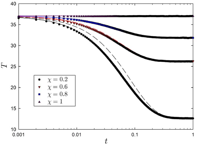
Figure 6.1: Direct relaxation of the granular temperature $T$ for different final noise amplitudes. All curves start from the stationary state corresponding to $\chi_{0}=1$. Monte Carlo simulations for a system of $N=100$ sites (symbols) are compared with the numerical solution of the first Sonine approximation (6.34) (solid lines), and the analytic solution of the linear response system (6.40) (dashed lines).

6.3.2 Kovacs hump

Since the numerical integration of the first Sonine approximation perfectly agrees with Monte Carlo simulations, we compare the analytical results for the Kovacs hump with the former. Specifically, we work in reduced variables, and therefore, we integrate numerically (6.38).

Linear response

It is convenient to rewrite the expression for the Kovacs hump in an alternative form to compare our theory with numerical results. We take advantage of the simple structure of the relaxation function in the first Sonine approximation, which is the sum of two exponentials, to introduce the factorization [109]

$$K_{T}(s)=K_{0}(s_{w})K_{1}(s-s_{w}),$$ (6.49a)

where

$$K_{0}(s_{w})=c_{+}c_{-}\frac{e^{\lambda_{+}s_{w}}-e^{\lambda_{-}s_{w}}}{1-\phi_{T}(s_{w})},\qquad K_{1}(s-s_{w})=e^{\lambda_{+}(s-s_{w})}-e^{\lambda_{-}(s-s_{w})}.$$ (6.49b)

Firstly, this factorization property shows that the position $s_{k}$ of the maximum relative to the waiting time $s_{w}$, that is, $s_{k}-s_{w}$, is controlled by the function $K_{1}$. Thus, $s_{k}-s_{w}$ does not depend on the waiting time, but only on the two eigenvalues $\lambda_{\pm}$. Namely,

$$s_{k}-s_{w}=\frac{1}{\lambda_{+}-\lambda_{-}}\ln\left(\frac{\lambda_{-}}{\lambda_{+}}\right)\underset{\beta=1}{\simeq}0.442.$$ (6.50)

Secondly, the height of the maximum $K_{\max}$ does depend on the waiting time $s_{w}$ due to the factor $K_{0}(s_{w})$. Specifically, it can be shown that $K_{\max}$ is a monotonically decreasing function of the waiting time $s_{w}$ that vanishes in the limit as $s_{w}\to\infty$.

In order to check the above results, we have fixed the initial and final drivings in the Kovacs protocol $\chi_{0}$ and $\chi$ and changed the intermediate driving value $\chi_{1}$. We do so to simplify the comparison, because the time scale $s$ involves the steady value of the temperature; see (6.37). Note that the smaller $\chi_{1}$ is, the shorter the waiting time becomes. Therefore, one expects to get a Kovacs hump whose maximum remains at $s-s_{w}\simeq 0.44$, but raises as $\chi_{1}$ decreases. This is shown in figure 6.2, where the numerical solution of the first Sonine approximation (6.38) and the analytical result (6.49) are compared. Their agreement is almost perfect for the two lowest curves, corresponding to $\chi_{1}=0.99$ and $\chi_{1}=0.95$, as expected, but is still remarkably good for the two topmost ones, corresponding to the not-so-small jumps for $\chi_{1}=0.8$ and $\chi_{1}=0.5$.

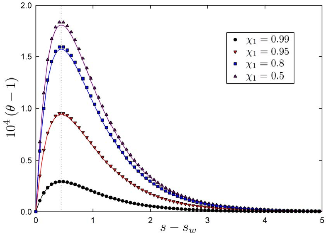
Figure 6.2: Kovacs hump in linear response. Initial and final drivings, $\chi_{0}=1.05$ and $\chi=1$ are fixed. We have considered four values for the intermediate driving, namely $\chi_{1}=\{0.5,0.8,0.95,0.99\}$. The linear response result (6.49) (solid line) perfectly agrees with the numerical solution of the first Sonine approximation (6.38) (symbols). In addition, we plot the theoretical prediction for the maximum (6.50), which again agrees with the numerics (dotted line).

Nonlinear regime

Furthermore, we explore the Kovacs effect out of the linear regime. Figure 6.3 is similar to figure 6.2, but for larger temperature (or driving) jumps. We have also fixed the initial and final values of the driving, $\chi_{0}=10$ and $\chi=1$. The intermediate values of the driving are the same as in the linear case except for the largest one, $\chi_{1}=0.99$, which we have omitted for the sake of clarity—its hump is too small in the scale of the figure. Now, the linear response theory results just provide the qualitative behavior of the hump, correctly predicting the position of the maximum, but not its height. On the one hand, and consistently with the numerical results in an active matter model [119], the Kovacs hump out of the linear response regime is larger than the prediction of linear response theory. On the other hand, the position of the maximum remains basically unchanged, and its height still increases as $\chi_{1}$ decreases.

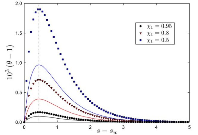
Figure 6.3: Kovacs hump in the nonlinear regime. The initial driving is much higher than that in figure 6.2, $\chi_{0}=10$, whereas the final and intermediate values of the driving are the same, $\chi=1$ and $\chi_{1}=\{0.5,0.8,0.95\}$. The linear response theoretical expression (6.44) (solid line) seriously underestimates the actual humps, given by the numerical solutions of the first Sonine approximation (6.38) (symbols). However, the theoretical prediction for the maximum position in linear response (6.50) (dotted line) is still quite accurate, see also figure 6.4.

We also compare our analytical expansion in $a_{2}^{\text{s}}$ with the numerical solutions of (6.38) for large jumps. Specifically, in order to make things as simple as possible, we choose $\chi_{1}=0$. If the waiting time is long enough, the system reaches the homogeneous cooling state and $a_{2}(s_{w})=a_{2}^{\text{HCS}}$, which is then the initial condition for the final stage of the Kovacs protocol. Moreover, we can compute the location of the maximum of the hump from (6.48), obtaining

$$s_{k}-s_{w}=\frac{2}{\kappa_{2}-2-\beta}\ln\left(\frac{2\kappa_{2}}{2+\beta}\right)\underset{\beta=1}{\simeq}0.437.$$ (6.51)

This result is numerically indistinguishable from that of linear response, as given by (6.50), since the relative error is around $1\%$.

In figure 6.4, we put forward a comparison between the Kovacs hump obtained from the numerical solution of the first Sonine approximation equations and our theoretical expression for the nonlinear regime, as given by (6.48). Fixing $\xi_{1}=0$ and $\xi=1$, as $\xi_{0}$ increases (as the waiting time is increased), the hump approaches (6.48) with $a_{2}^{\text{ini}}=a_{2}^{\text{HCS}}$. Moreover, our theory perfectly reproduces all the simulations when we substitute the actual values of $a_{2}^{\text{ini}}$ into (6.48).

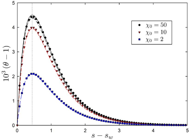
Figure 6.4: Kovacs hump in the nonlinear regime. We have considered the following values of the drivings: $\chi_{0}=\{2,10,50\}$, $\chi_{1}=0$ and $\chi=1$. Symbols stand for the numerical solutions of the first Sonine approximation (6.38), whereas lines correspond to the theoretical expression stemming from a perturbative expansion in $a_{2}^{s}$, as given by (6.48). For the solid line, $a_{2}^{\text{ini}}=a_{2}^{\text{HCS}}$, whereas we have used the value of $a_{2}^{\text{ini}}$ in the numerical solution for the dashed lines. An almost perfect agreement is observed. Finally, we  also mark the theoretical prediction for the maximum position in nonlinear response (6.51) (dotted line), which also shows an excellent agreement with the numerics.

6.3.3 Time evolution of the $H$-functional

The nonmonotonicity in the relaxation of the granular temperature that is brought about by the Kovacs protocol is not automatically transferred to other relevant physical magnitudes. Specifically, here, we deal with the $H$-functional

$$H(t)=\int_{-\infty}^{+\infty}dvP_{1}(v,t)\log\left[\frac{P_{1}(v,t)}{P_{1}^{(\text{s})}(v)}\right],$$ (6.52)

which we have analyzed in chapter 5. Therein, we have analytically proven that $H(t)$ is a Lyapunov functional in our system for the Maxwell collision rule, which corresponds to the case $\beta=0$. However, it is precisely for this case that the Kovacs effect vanishes, since the evolution equation for the temperature is closed. Therefore, we look into the time evolution of $H(t)$ for the hard particle case $\beta=1$ in this section. Note that, in addition to our rigorous proof in the model for the Maxwell case, there is strong numerical evidence of $H(t)$ being a Lyapunov functional for granular systems [97, 98].

We have computed $H(t)$ numerically from (6.52) within the first Sonine approximation, that is, we have substituted both $P_{1}(v,t)$ and $P_{1}^{(\text{s})}(v)$ by their expressions in the first Sonine approximation and calculated the integral numerically. This has been done for the Kovacs protocols considered in figures  6.2 and 6.3. The results are shown in figure 6.5 and make it clear that $H(t)$ still monotonically decreases for the Kovacs-like protocols, in both the linear (top panel) and nonlinear (bottom panel) regimes. At the time of the maximum in the hump, $s-s_{w}\simeq 0.44$, no special signature is observed in the “entropy”, which would be given by $-k_{B}H(t)$.

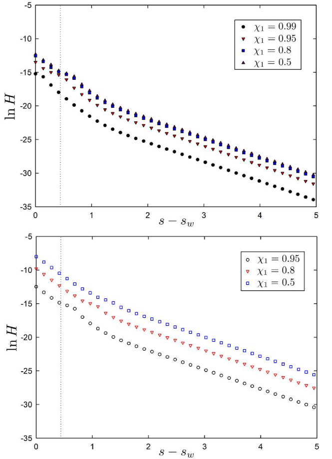
Figure 6.5: Time evolution of the $H$-functional in the Kovacs experiments. The top and bottom panels correspond, respectively, to the protocols in figures 6.2 (filled symbols) and 6.3 (open symbols), that is, to the linear and nonlinear regimes. The vertical dotted line marks the maximum of the hump in the corresponding regime.

Chapter 7 Conclusions

This thesis intends to be a showcase for the relevance of simple models as useful tools for improving our understanding of complex systems. We have analyzed, mainly, two models of very different nature with the fundamental tools of the statistical mechanics. On the one hand, we have studied a model capable of predicting the deterministic unfolding pathway in modular biomolecules. On the other hand, we have thoroughly explored a model with nonconservative interactions, motivated within the field of soft matter and granular media.

In this final chapter we enumerate the major conclusions of this thesis as well as some future perspectives. Regarding the first part devoted to the biophysical model:

1. We have put forward a 1d model for modular biomolecules that comprises several consecutive nonharmonic units, which is submitted to a mechanical pull that tries to control the total length of the chain. Langevin dynamics is assumed for the endpoints of the different units.

2. Dynamical equations are solved, in the limit of negligible thermal noise, by means of a perturbative approach in both the pulling velocity and the asymmetry between units. Within this quite drastic approach, the dynamics becomes deterministic. With no thermal activation being allowed, the only mechanism for unfolding is reaching the stability threshold, where the folded state ceases to exist.

3. We derive the critical values of the pulling velocity at which the unfolding pathway changes. For slow enough pulling, it is the weakest unit the first to unfold. By contrast, for fast enough pulling, the first unit to unfold is the closest to the pulled end. Intermediate situations are also possible, depending on the details of the system. Comparison between numerical solutions of specific systems and theoretical predictions shows a remarkably good agreement.

4. The applicability of the model has been carefully looked into. The pulling velocity has to lie within a very specific range: low enough to make our perturbative approach possible, and, at the same time, high enough to prevent thermal activation and make the system follow the maximum hysteresis path. These conditions make it difficult to choose the “right” molecule to test our theory.

5. The robustness of the theoretical model has been tested by varying the model in different ways. The described phenomenology does not depend on the details of the pulling device. Specifically, we have analyzed both the impact of the location of the elastic reaction of the pulling device and the finite value of its stiffness. The latter leads to an imperfect control of the length.

6. Steered molecular dynamics of a model system composed of two consecutive coiled-coil structures have been performed. The statistical study of the trajectories reveals (i) an excellent agreement with the theoretical prediction for high enough pulling velocities and (ii) anisotropic behavior of the molecule.

7. We have limited ourselves to the investigation of the first unfolding event. However, our argument can be easily generalized to the next unfolding event: the difference is that the zero-th order approximation is no longer given by all the units sweeping the all-units-folded branch, but by the sweeping of the branch with one module unfolded and the remainder folded. Then, a similar perturbative expansion around this zero-th order solution, in powers of the asymmetry and the pulling speed, would give the next unit that opens.

8. Although we focus on the biophysical application of this model, it is worth highlighting that similar models have been employed in other fields. Many physical systems are also “modular”, since they comprise several units [42], and thus a similar phenomenology may emerge. Some examples can be found in studies of plasticity [186, 187], lithium-ion batteries [188, 189], and ferromagnetic alloys [190].

9. Finally, we briefly comment on some prospects for future work:

   1. As stressed throughout the thesis, we have considered the deterministic approximation of the Langevin dynamics. Including temperature effects, in a way similar to that of Kramers theory [35, 36, 37, 38], would complete our theoretical approach.

   2. We assume that the dynamical stability threshold equals that of the static case. We have discussed how seeking a dynamical criterion could lead to an improvement of our theory, reducing its discrepancies with the numerical results.

   3. After analyzing in detail the unfolding scenario in a simple molecule such as the two coiled-coil construct, the next natural step is exploring more complex molecules, in which the modules are not identical. Therein, we expect the emergence of the predicted critical velocities.

   4. Once simulations have supported our theoretical prediction, the desirable continuation would be going to real experiments. In the current state of the theory, where thermal activation is neglected, the difficulties of this stage are neat: the test molecule should be carefully chosen.

Concerning the second part devoted to the granular model:

1. We have analyzed a simple model for the “transversal” component of the velocity of a granular fluid. The model captures many of the essential features of granular fluids, for example the existence of some characteristic “basic” states like the Homogeneous Cooling State and the Uniform Shear Flow steady state.

2. Specifically, we have focused on the continuum limit of the one-particle distribution function and its solutions. In this regard, we would like to stress that we have completely characterized the Homogeneous Cooling State and the Uniform Shear Flow steady state. Also, we have compared, with excellent results, our theoretical predictions with numerical simulations.

3. We have looked into the relevant fluctuating fields of the model. Some of them need a proper regularization since their definitions in the continuum limit lead to singularities. This issue, although known in the literature [191], is neatly understood within our theoretical framework.

4. We have exactly solved the average two-particle correlations in a system of arbitrary size, by reducing the solution of the evolution equations to an eigenproblem. The obtained spectrum is particularly interesting, since it allows us to explain the shear instability of the system as the crossing of the two first eigenvalues. Moreover, it improves our understanding of the situation beyond the instability ($\nu>\nu_{c}$) in the model: we find that both the energy and the correlations still decay to zero but with a rate that is independent of the inelasticity.

5. The $H$-theorem we have derived here is, to the best of our knowledge, the first rigorous proof of its kind in systems with nonconservative interactions. Not only have we proven the global stability of a family of nonequilibrium steady solutions in our simplified model, but also understood why the “Boltzmann entropy” $H_{B}$ cannot be a good candidate for a Lyapunov functional in inelastic systems. In addition, our work strongly supports previous numerical evidence [98, 97] in favor of the master-equation-like $H$-functional being the “correct” Lyapunov functional in the granular case.

6. The ideas introduced in our proof of the $H$-theorem (expansion of the distribution and splitting of the evolution operator) could be useful in more complex systems, closer to the real granular gas. If this extension is not possible, one would like, at least, to show that the long-time solutions are globally stable by establishing that $H$ is asymptotically nonincreasing, similarly to what has been done in this thesis.

7. Also, we have analyzed Kovacs-like memory effects in our model. We have done so by introducing a kinetic approach—specifically, a Sonine expansion—in our model. This Sonine expansion makes it possible to close the temperature equation together with that for the excess kurtosis. Theoretical predictions for the linear response have been successfully validated by the numerical results. We have also checked that the nonmonotonic behavior of the temperature in the Kovacs experiment is utterly compatible with the monotonic decrease of the $H$-functional to its steady value.

8. The theoretical framework developed for the study of memory effects here goes beyond its application to our model. In particular, it establishes the basis for a general approach to this kind of memory effects, within linear response, in athermal systems. In this regard, it is worth emphasizing that our approach is very general, since it works both at the mesoscopic and macroscopic levels of description.

9. Also for the granular part of the thesis, we discuss some possibilities for further development:

   1. Throughout the thesis, we have focused on the study of the “Maxwellian” case $\beta=0$ of our granular model. The investigation of the general case for $\beta\neq 0$ is worthy of further consideration. In particular, the case $\beta=1$ leads to a collision rate analogous to that of hard particles. For instance, the nonequilibrium stationary states in the general case are more involved and deserve to be analyzed in depth.

   2. Considering other physically relevant energy injection mechanisms would extend the applicability of the model. This generalization could lead us closer to a “master” lattice model, which merge the results stemming from this thesis with other works, as those in [177].

   3. One of the most appealing future prospects is the possibility of exploring a derivation of global stability or even an $H$-theorem for the inelastic Boltzmann equation, by using ideas similar to those presented in chapter 5.

   4. A complete theoretical description of the Kovacs effect out of the linear response regime is lacking. Extending our results to the nonlinear regime would be, undoubtedly, of utmost relevance in nonequilibrium physics.

Appendix A Stability threshold

To first order in $\xi$, the extension $x_{i,b}$ such that $a^{\prime\prime}_{i}(x_{i,b})=0$ verifies

$$a^{\prime\prime\prime}(\ell_{b})(x_{i,b}-\ell_{b})+\xi\delta\!f^{\prime}_{i}(\ell_{b})=0,$$ (A.1)

that is,

$$x_{i,b}=\ell_{b}-\xi\frac{\delta\!f^{\prime}_{i}(\ell_{b})}{a^{\prime\prime\prime}(\ell_{b})}.$$ (A.2)

The corresponding force at the stability threshold is obtained from (2.11). To the lowest order in the deviations,

$$F_{i,b}\equiv a^{\prime}_{i}(x_{i,b})\sim a^{\prime}_{i}(\ell_{b})=F_{b}+\xi\,\delta\!f_{i}(\ell_{b}),$$ (A.3)

because the next term, $a^{\prime\prime\prime}(\ell_{b})(x_{i,b}-\ell_{b})^{2}/2$, is of the order of $\xi^{2}$. Therefore, the $i$-th module reaches its limit of stability at the time for which $x_{i}=x_{i}^{(0)}+\xi\delta x_{i}=x_{i,b}$, that is, when the length per unit $\ell$ has the value $\ell_{i}$ verifying

$$\ell_{i}+\xi\frac{\overline{\delta\!f}(\ell_{i})-\delta\!f_{i}(\ell_{i})}{a^{\prime\prime}(\ell_{i})}=\ell_{b}-\xi\frac{\delta\!f^{\prime}_{i}(\ell_{b})}{a^{\prime\prime\prime}(\ell_{b})},$$ (A.4)

or, equivalently,

$$\ell_{i}-\ell_{b}=\xi\frac{\delta\!f_{i}(\ell_{i})-\overline{\delta\!f}(\ell_{i})}{a^{\prime\prime}(\ell_{i})}-\xi\frac{\delta\!f^{\prime}_{i}(\ell_{b})}{a^{\prime\prime\prime}(\ell_{b})}.$$ (A.5)

We know that $\ell\to\ell_{b}$ when $\xi\to 0$. But $a^{\prime\prime}(\ell_{b})=0$ and thus we cannot substitute $\ell_{b}$ on the rhs of (A.5). On the other hand, this means that the dominant balance for $\xi\to 0$ involves the lhs and the first term on the rhs of (A.5). Therefore, making use of $a^{\prime\prime}(\ell)\sim a^{\prime\prime\prime}(\ell_{b})(\ell-\ell_{b})$, we get

$$(\ell_{i}-\ell_{b})^{2}\sim\xi\frac{\delta\!f_{i}(\ell_{b})-\overline{\delta\!f}(\ell_{b})}{a^{\prime\prime\prime}(\ell_{b})}.$$ (A.6)

Since $a^{\prime\prime\prime}(\ell_{b})<0$ (see figure 2.2), this means that only the units with $\delta\!f_{i}(\ell_{b})$ smaller than the average (that is, weaker than average) reach the limit of stability in the limit as $v_{p}\to 0$. In fact, it is the weakest unit, that is, the unit with smallest $\delta\!f_{i}(\ell_{b})$, that unfolds first.

It is interesting to note that, in order to obtain (A.6), we have completely neglected the last term on the rhs of (A.5). Since, in turn, this term stems from the last term on the rhs of (A.2), to the lowest order we are solving the equation $x_{i}=\ell_{b}$. In other words, to the lowest order the stability threshold can be considered to be given by the non-disordered, zero-asymmetry case, free energy $a(x)$. For the sake of concreteness and simplicity, we have stuck to the asymmetry contribution $\delta x_{i}$ in this appendix, but the same condition $x_{i}=\ell_{b}$ would still be valid, had we taken into account the kinetic contribution $\Delta x_{i}$ derived in section 2.2.2. The reason is that there is also a factor $a^{\prime\prime}(\ell)$ in the denominator of $\Delta x_{i}$, see (2.24a), and thus both the terms coming from $\delta x_{i}$ and $\Delta x_{i}$ are dominant against the last term on the rhs of (A.2).

Appendix B Fluctuating expression for the dissipation

Let us consider the dissipation $d_{l,p}$ at site $l$ and at time $p$. Its main part is obtained by averaging (4.6) with respect to the fast variables $y_{p}$, i.e.

$$\bar{d}_{l,p}=\frac{\alpha^{2}-1}{4L}\left(\Delta_{l,p}^{2}+\Delta_{l-1,p}^{2}\right)<0.$$ (B.1)

This is the expression that we have to analyze in the fluctuating hydrodynamic description, since the amplitude of the dissipation noise scales as $L^{-3}$ [150, 151]. If we consider the average of the dissipation field, it is readily obtained that $d^{\text{av}}_{l,p}=(\alpha^{2}-1)T_{l,p}/L$, which gives (4.13) in the continuum limit by using $d(x,t)=L^{3}d_{l,p}$ and the definition of $\nu$. Therefore, it is consistent to write at the fluctuating level that

$$\bar{d}_{l,p}=\frac{\alpha^{2}-1}{L}\theta_{l,p},$$ (B.2)

by defining the fluctuating temperature as

$$\theta_{l,p}=\frac{1}{4}\left(\Delta_{l,p}^{2}+\Delta_{l-1,p}^{2}\right)=\frac{v_{l-1,p}^{2}+2v_{l,p}^{2}+v_{l+1,p}^{2}}{4}-v_{l,p}\frac{v_{l+1,p}+v_{l-1,p}}{2}.$$ (B.3)

The first term on the rhs, $(v_{l-1,p}^{2}+2v_{lp}^{2}+v_{l+1,p}^{2})/4$, reduces to $e_{l,p}$ plus terms of the order of $L^{-2}$, which are neglected.

Our main goal is to obtain a correct expression for $v_{l,p}v_{l\pm 1,p}$ at the fluctuating level. In general, we have for the average correlations

$$\langle v_{l,p}v_{l^{\prime},p}\rangle=E_{l,p}\delta_{ll^{\prime}}+C_{l,l^{\prime}-l;p}\left(1-\delta_{ll^{\prime}}\right),$$ (B.4)

with the definition

$$C_{l,l^{\prime}-l;p}=\langle v_{l,p}v_{l^{\prime},p}\rangle\quad\text{for $l^{\prime}\neq l$}.$$ (B.5)

The functions $C_{k,p}$ defined in section 4.5 are the particularisation of $C_{l,l^{\prime}-l;p}$ to a homogeneous situation ($k=l^{\prime}-l$). Consistently with (B.4), we write

$$v_{l,p}v_{l^{\prime},p}=e_{l,p}\delta_{ll^{\prime}}+\gamma_{l,l^{\prime}-l,p}\left(1-\delta_{ll^{\prime}}\right)=\gamma_{l,l^{\prime}-l,p}+\left(e_{l,p}-\gamma_{l,l^{\prime}-l,p}\right)\delta_{ll^{\prime}},$$ (B.6)

at the fluctuating level. We have introduced the fluctuating correlations $\gamma_{l,l^{\prime}-l,p}$, such that $\langle\gamma_{l,l^{\prime}-l;p}\rangle=C_{l,l^{\prime}-l,;p}$. In the continuum limit, $x=(l-1)/L$ and $x^{\prime}=(l^{\prime}-1)/L$ and (B.6) is transformed into

$$v(x,t)v(x^{\prime},t)=\gamma(x,x^{\prime}-x;t)+L^{-1}\delta(x-x^{\prime})\left[e(x,t)-\gamma(x,x^{\prime}-x;t)\right],$$ (B.7)

because $\delta_{l,l^{\prime}}\sim L^{-1}\,\delta(x-x^{\prime})$, see note at the end of the appendix.

Taking into account (B.3) and the above definitions, the fluctuating temperature in the continuum limit is

$$\theta(x,t)=e(x,t)-\gamma(x,0;t),$$ (B.8)

where we have neglected terms of the order of $L^{-2}$. Since we are interested in the limit of $\gamma(x,\Delta x;t)$ when $\Delta x\to 0$, we use (B.7) with $\Delta x=x^{\prime}-x=\pm L^{-1}$ to obtain

$$v^{2}(x,t)=\gamma(x,0;t)+L^{-1}\left[e(x,t)-\gamma(x,0;t)\right]\lim_{x^{\prime}\to x}\delta(x^{\prime}-x).$$ (B.9)

Thus, we have that

$$\gamma(x,0;t)=v^{2}(x,t)-L^{-1}\theta(x,t)\lim_{x^{\prime}\to x}\delta(x^{\prime}-x).$$ (B.10)

Note that $v^{2}(x,t)$ always has a singular part that stems from the $\delta(\Delta x)$ factors on the rhs of (B.9). Therefore, $\gamma(x,0;t)$ can be considered as the “regular” part of $v^{2}(x,t)$, and we introduce the notation

$$v_{R}^{2}(x,t)\equiv\gamma(x,0;t)=v^{2}(x,t)-L^{-1}\theta(x,t)\lim_{x^{\prime}\to x}\delta(x^{\prime}-x).$$ (B.11)

By combining the previous results, and recalling that $d(x,t)=L^{3}d_{l,p}$, we finally conclude

$$d(x,t)=-\nu\theta(x,t),\quad\theta(x,t)=e(x,t)-v_{R}^{2}(x,t).$$ (B.12)

This tells us that the fluctuations of the dissipation field are enslaved to those of the temperature. Moreover, the appearance of $v_{R}^{2}$ in (B.12) is easy to understand on a physical basis, since $\langle v_{R}^{2}(x,t)\rangle=\langle\gamma(x,0;t)\rangle=u^{2}(x,t)+O(L^{-1})$. Equations (B.11) and (B.12) make it possible to write a closed expression for the fluctuating temperature,

$$\theta(x,t)=\beta\left[e(x,t)-v^{2}(x,t)\right],\quad\beta=\left[1-L^{-1}\lim_{x^{\prime}\to x}\delta(x^{\prime}-x)\right]^{-1},$$ (B.13)

in which $\beta$ is a regularisation factor, which “heals” the singularity of $v^{2}(x,t)$ in the large system size limit.

Note: The appearance of $\delta(0)$—more accurately, $\lim_{x^{\prime}\to x}\delta(x^{\prime}-x)$—can be avoided in the following way: for discrete $(l,l^{\prime})$ we may write

$$\delta_{ll^{\prime}}=\Theta(l-l^{\prime}+1/2)\Theta(l^{\prime}-l+1/2),$$ (B.14)

in which $\Theta(x)$ is the Heaviside step function. Therefore, in the continuum limit, we have that

$$\delta_{ll^{\prime}}\sim\Theta\left(x-x^{\prime}+\frac{1}{2L}\right)\Theta\left(x^{\prime}-x+\frac{1}{2L}\right).$$ (B.15)

When used inside an integral, the relative error introduced by using the expression above is of the order of $L^{-2}$, since

$$\sum_{l=1}^{L}f_{l}\,\delta_{ll^{\prime}} =f_{l^{\prime}},$$ (B.16)

$$L\int_{0}^{1}dxf(x)\,\Theta\left(x-x^{\prime}+\frac{1}{2L}\right)\Theta\left(x^{\prime}-x+\frac{1}{2L}\right) =\int_{x^{\prime}-\frac{1}{2L}}^{{x^{\prime}+\frac{1}{2L}}}dx\,f(x)$$

$$=f(x^{\prime})+O(L^{-2}).$$ (B.17)

Therefore, both expressions, (i) $L^{-1}\delta(x-x^{\prime})$ and (ii) the product of Heaviside functions, can be used indistinctly within the mesoscopic fluctuation framework.

Consistently with the above discussion, the Fourier components of the product of Heaviside functions are the same as those of $L^{-1}\delta(x-x^{\prime})$, with a relative error of the order of $L^{-2}$,

$$\int_{0}^{1}dx\,\Theta\left(x-x^{\prime}+\frac{1}{2L}\right)\Theta\left(x^{\prime}-x+\frac{1}{2L}\right)e^{-ik_{n}x} =\int_{x^{\prime}-\frac{1}{2L}}^{{x^{\prime}+\frac{1}{2L}}}dxe^{-ik_{n}x}$$

$$=L^{-1}e^{-ik_{n}x^{\prime}}+O(L^{-3}).$$ (B.18)

Therefore,

$$\Theta\left(x-x^{\prime}+\frac{1}{2L}\right)\Theta\left(x^{\prime}-x+\frac{1}{2L}\right) =L^{-1}\sum_{n}e^{ik_{n}(x-x^{\prime})}+O(L^{-3})$$

$$=L^{-1}\delta(x-x^{\prime})+O(L^{-3}).$$ (B.19)

Appendix C Simulation method

Simulations have been made reproducing $M$ times the phase-space trajectory of a system of $N$ particles, each one carrying a velocity $v_{l}$ and being at a definite position $l=1,\ldots,L$, with $L=N$ for periodic or Lees-Edwards boundaries. For each trajectory, the system starts with a random extraction of velocities $v_{l}$ normally distributed with $\left\langle v_{l}\right\rangle=0$ and $\left\langle v^{2}_{l}\right\rangle=T_{0}$, unless otherwise specified. Afterwards, we move to the centre of mass frame making the transformation $v_{l}\Rightarrow v^{\prime}_{l}=v_{l}-\frac{1}{L}\sum^{L}_{l=1}v_{l}$, so that the total momentum of the system is zero.

We carry out the Monte Carlo simulation of the system time-evolution through the residence time algorithm, which gives the numerical integration of a master equation in the limit of infinite trajectories [192, 193]. The basic numerical recipe is as follows:

1. At time $\tau$, a random “free time” $\tau_{f}>0$ is extracted with an exponential probability density $\Omega(\bm{v})\exp[-\Omega(\bm{v})\tau_{f}]$, where $\Omega(\bm{v})=\sum_{l}\omega|v_{l}-v_{l+1}|^{\beta}$ depends on the state of the system $\bm{v}$;

2. Time is advanced by such a free time $\tau\to\tau+\tau_{f}$;

3. A pair $(l,l+1)$ is chosen to collide with probability $\omega|v_{l}-v_{l+1}|^{\beta}/\Omega(\bm{v})$;

4. The chosen pair collide following the collision rule (4.1).

5. In the case of the thermostated system, all particles are heated by the stochastic thermostat, by adding independent Gaussian random numbers of zero mean and variance $\chi\tau_{f}$ to their velocities;

6. In the case of the thermostated system, the mean value of the random numbers generated in the previous step is subtracted from the velocities of all particles to conserve momentum;

7. The process is repeated from Step 1.

Regarding the measurement of $P_{1}(v;x,t)$, we sample both position and velocity spaces by defining $N_{x}$ bins of width $\Delta x$ and $N_{v}$ bins of with $\Delta v$. Of course, the product $N_{x}\Delta x=1$, covering the whole lattice, whereas $N_{v}\Delta v$ gives the range of velocities bounded by the cutoffs $v_{\text{\text{min}}}$ and $v_{\text{max}}$. In our simulations, we control that the contribution to the PDFs coming from velocities outside the considered interval $[v_{\text{min}},v_{\text{max}}]$ is negligible. With such a binning, we build up an histogram and therefrom the distribution function $P_{1}(v;x,t)$, which is represented by a $N_{x}\times N_{v}$ matrix for each time $t$. Functionals ($H$ and $H_{B}$) are computed by numerically replacing the integral over $x$ and $v$ with sums over the prescribed bins.

Appendix D Lees-Edwards boundary conditions

Here, we derive the Lees-Edwards boundary conditions in the continuum limit (4.40), starting from the collision rules for the boundary sites of our lattice. As stated in section 4.3.2, the collision rule for the pair $(1,L)$ is

$$v_{L,p+1} =v_{L,p}-\frac{1+\alpha}{2}(v_{L,p}-v_{1,p}-a),$$ (D.1a)

$$v_{1,p+1} =v_{1,p}+\frac{1+\alpha}{2}(v_{L,p}-a-v_{1,p}),$$ (D.1b)

which, as the bulk rule (4.1), conserves momentum. The evolution equation for $v_{1}$ is readily obtained,

$$v_{1,p+1}-v_{1,p}=-\frac{1+\alpha}{2}\delta_{y_{p},1}(v_{1,p}-v_{2,p})+\frac{1+\alpha}{2}\delta_{y_{p},L}(v_{L,p}-a-v_{1,p}),$$ (D.2)

whereas for the energy we have

$$e_{1,p+1}-e_{1,p}= -(1+\alpha)v_{1,p}(v_{1,p}-v_{2,p})\delta_{y_{p},1}+(1+\alpha)v_{1,p}(v_{L,p}-a-v_{1,p})\delta_{y_{p},L}$$

$$+\left(\frac{1+\alpha}{2}\right)^{2}\left(v_{1,p}-v_{2,p}\right)^{2}\delta_{y_{p},1}+\left(\frac{1+\alpha}{2}\right)^{2}\left(v_{L,p}-a-v_{1,p}\right)^{2}\delta_{y_{p},L}.$$ (D.3)

Taking averages in (D.2) and (D), we get

$$u_{1,p+1}-u_{1,p} =\frac{1+\alpha}{2L}(u_{L,p}-a-2u_{1,p}+u_{2,p}),$$ (D.4a)

$$E_{1,p+1}-E_{1,p} =\frac{1+\alpha}{L}\left(\left\langle v_{L,p}v_{1,p}\right\rangle-au_{1,p}-2E_{1,p}+\left\langle v_{1,p}v_{2,p}\right\rangle\right)$$

$$+\frac{(1+\alpha)^{2}}{4L}\left(2E_{1,p}+2E_{2,p}+a^{2}-2\left\langle v_{L,p}v_{1,p}\right\rangle\right.$$

$$\qquad\qquad\qquad\left.-2\left\langle v_{1,p}v_{2,p}\right\rangle-2au_{1,p}-2au_{L,p}\right).$$ (D.4b)

Now, we turn our attention to the continuum limit defined in (4.9). Specifically, we identify $f_{l,p}=f\left[x=(l-1)/L,t=p/L^{3}\right]$, being $f(x,t)$ a “smooth” function. Therefore,

$$f_{1,p} =f(0,t),$$ (D.5a)

$$f_{1,p+1} =f(0,t+1/L^{3})=f(0,t)+L^{-3}\partial_{t}f(0,t)+\mathcal{O}\left(L^{-6}\right),$$ (D.5b)

$$f_{2,p} =f(1/L,t)=f(0,t)+L^{-1}\left.\partial_{x}f(x,t)\right|_{x=0}+\mathcal{O}\left(L^{-2}\right),$$ (D.5c)

$$f_{L,p} =f(1-1/L,t)=f(1,t)-L^{-1}\left.\partial_{x}f(x,t)\right|_{x=1}+\mathcal{O}\left(L^{-2}\right).$$ (D.5d)

Substituting (D.5) into (D.4), and using that

$$\frac{1+\alpha}{2}=1+\mathcal{O}\left(L^{-2}\right),$$ (D.6)

one can obtain, after some algebra,

$$0 =u(1,t)-u(0,t)-a+L^{-1}\left[\left.\partial_{x}u(x,t)\right|_{x=1}-\left.\partial_{x}u(x,t)\right|_{x=1}\right]+\mathcal{O}\left(L^{-2}\right),$$ (D.7a)

$$0 =E(1,t)-E(0,t)-2au(1,t)+a^{2}$$

$$\,\quad+L^{-1}\left[\left.\partial_{x}E(x,t)\right|_{x=0}-\left.\partial_{x}E(x,t)\right|_{x=1}+2a\left.\partial_{x}u(x,t)\right|_{x=1}\right]+\mathcal{O}\left(L^{-2}\right).$$ (D.7b)

Above, as explicitly notated, we have only retained the two lowest orders in the expansion in powers of $L^{-1}$. Imposing that the considered orders vanish separately and taking into account the definition of the temperature, as given by (4.10), finally lead us to the boundary conditions in (4.40).

Appendix E Derivation of the expression for $dH/dt$ in a general driven state

Let us consider the three contributions to $dH/dt$ in (5.15). We start with the diffusive one,

$$\left.\frac{dH}{dt}\right|_{\text{diff}}=\int\!\!dx\,dv\,\left(\mathcal{L}_{\text{diff}}P_{1}\right)\,\ln\left(\frac{P_{1}}{P_{1}^{(s)}}\right)-\int\!\!dx\,dv\,\frac{P_{1}}{P_{1}^{(s)}}\,\mathcal{L}_{\text{diff}}P_{1}^{(s)},$$ (E.1)

where $\mathcal{L}_{\text{diff}}P_{1}=\partial_{xx}{P_{1}}$ and we have used that $\int\!\!dx\,dv\,\partial_{xx}{P_{1}^{(s)}}$ vanishes identically. Integrating by parts the first term on the rhs of (E.1), the result is

$$\int\!\!dv\,\partial_{x}{P_{1}}\left.\ln\left(\frac{P_{1}}{P_{1}^{(s)}}\right)\right|_{0}^{1}-\int\!\!dx\,dv\,P_{1}\partial_{x}{\ln P_{1}}\left(\partial_{x}{\ln P_{1}}-\partial_{x}{\ln P_{1}^{(s)}}\right).$$ (E.2)

Also integrating by parts the second term, one obtains

$$-\int\!\!dv\,\left.\frac{P_{1}}{P_{1}^{(s)}}\partial_{x}{P_{1}^{(s)}}\right|_{0}^{1}+\int\!\!dx\,dv\,P_{1}\partial_{x}{\ln P_{1}^{(s)}}\left(\partial_{x}{\ln P_{1}}-\partial_{x}{\ln P_{1}^{(s)}}\right).$$ (E.3)

We assume that the boundary terms are equal to zero, that is,

$$\int\!\!dv\,\left[\partial_{x}{P_{1}}\ln\left(\frac{P_{1}}{P_{1}^{(s)}}\right)-\frac{P_{1}}{P_{1}^{(s)}}\partial_{x}{P_{1}^{(s)}}\right]_{0}^{1}=0.$$ (E.4)

This is obviously true for Lees-Edwards and periodic boundary conditions. For the Couette state, in which the PDF at the boundaries is Gaussian with zero average velocity and a given temperature $T_{B}$ for all times, the first term is identically zero and the second vanishes because $\int\!\!dv\,P_{1}^{(s)}(v;x)=1$ for all $x$. Summing the two contributions to the diffusive term above, we have

$$\left.\frac{dH}{dt}\right|_{\text{diff}}=\int\!\!dx\,dv\,P_{1}\left(\partial_{x}{\ln P_{1}}-\partial_{x}{\ln P_{1}^{(s)}}\right)^{2},$$ (E.5)

which is (5.16) of the main text.

The noise term is treated along the same lines as above, but integrating by parts in $v$ instead of $x$, since $\mathcal{L}_{\text{noise}}P_{1}=\frac{\xi}{2}\partial_{v}^{2}{P_{1}}$. Therein, the boundary terms vanish if $P_{1}$ and $P_{1}^{(s)}$ tend to zero fast enough for $v\to\pm\infty$, and

$$\left.\frac{dH}{dt}\right|_{\text{noise}}=\int\!\!dx\,dv\,P_{1}\left(\partial_{v}{\ln P_{1}}-\partial_{v}{\ln P_{1}^{(s)}}\right)^{2},$$ (E.6)

which is (5.18).

Now we focus on the inelastic contribution,

$$\left.\frac{dH}{dt}\right|_{\text{inel}}=\int\!\!dx\,dv\,\left(\mathcal{L}_{\text{inel}}P_{1}\right)\,\ln\left(\frac{P_{1}}{P_{1}^{(s)}}\right)-\int\!\!dx\,dv\,\frac{P_{1}}{P_{1}^{(s)}}\,\mathcal{L}_{\text{inel}}P_{1}^{(s)},$$ (E.7)

in which $\mathcal{L}_{\text{inel}}P_{1}=\frac{\nu}{2}\partial_{v}{[(v-u)P_{1}]}$. Then,

$$\left.\frac{dH}{dt}\right|_{\text{inel}} =\;\frac{\nu}{2}\int\!\!dx\,dv\,\left\{\partial_{v}{[(v-u)P_{1}]}\right\}\,\ln\left(\frac{P_{1}}{P_{1}^{(s)}}\right)$$

$$\,\quad-\frac{\nu}{2}\int\!\!dx\,dv\,\left\{\partial_{v}{[(v-u_{s})P_{1}^{(s)}]}\right\}\,\frac{P_{1}-P_{1}^{(s)}}{P_{1}^{(s)}}.$$ (E.8)

Again, integrating by parts in $v$ (here we do not write the boundary terms at $v\to\pm\infty$), the first term on the rhs of (E.8) is

$$-\frac{\nu}{2}\int\!\!dx\,dv\,(v-u)P_{1}\,\left(\partial_{v}{\ln P_{1}}-\partial_{v}{\ln P_{1}^{(s)}}\right),$$ (E.9)

whereas the second term gives

$$\frac{\nu}{2}\int\!\!dx\,dv\,(v-u_{s})P_{1}\,\left(\partial_{v}{\ln P_{1}}-\partial_{v}{\ln P_{1}^{(s)}}\right).$$ (E.10)

Summing up these two contributions, and taking into account that both $u$ and $u_{s}$ do not depend on $v$,

$$\left.\frac{dH}{dt}\right|_{\text{inel}}=\frac{\nu}{2}\int\!\!dx\,(u-u_{s})\int\!\!dv\,P_{1}\left(\partial_{v}{\ln P_{1}}-\partial_{v}{\ln P_{1}^{(s)}}\right)$$ (E.11)

Since $\int\!dv\,P_{1}\,\partial_{v}{\ln P_{1}}\equiv\int\!dv\,\partial_{v}{P_{1}}=0$, this leads to (5.17).

Appendix F Completion of the proof of global stability

Here, we complete the proof of the global stability for $\xi=0$. In that case, (5.18) identically vanishes and the proof presented in the main text for deriving $\phi(v;t)=1$ in (5.21) does not hold.

For $\xi=0$, one can use the kinetic equation in the limit as $t\to\infty$, that is,

$$\lim_{t\to\infty}\frac{\partial\phi(v;t)}{\partial t}=\frac{\nu}{2}[v-u_{\text{s}}(x)]\lim_{t\to\infty}\frac{\partial\phi(v;t)}{\partial v}.$$ (F.1)

Since $\phi(v;t)$ has no spatial dependence, the limit of its time derivative must vanish and, consistently, the same applies for its velocity derivative. In this way, $\phi(v;t)=1$ is reobtained, by employing (5.21) and the normalization of the distributions.

The above result can be proven by a reductio ad absurdum argument. If the long time limit of $\partial_{v}\phi(v,t)$ were nonzero, we would show $u_{s}(x)$ to depend only on $v$ by solving (F.1) for $u_{s}(x)$. This is contradictory, thus $\lim_{t\rightarrow\infty}\partial_{v}\phi(v,t)$ must vanish and so must $\lim_{t\rightarrow\infty}\partial_{t}\phi(v,t)$, by taking into account again (F.1).

Note that the argument in the previous paragraph ceases to be valid in case of a homogeneous $u_{\text{s}}$. However, the only possible flat profile is $u_{\text{s}}=0$, and this implies a null shear rate. Were that the case, both $a$ and $\xi$ would vanish and no energy injection mechanism would be present: in a few words, no stationary state would be attained.

List of acronyms

LOT

Laser optical tweezers

AFM

Atomic force microscopy

FJC

Freely-jointed chain

WLC

Worm-like chain

MBP

Maltose binding protein

PDB

Protein data bank

HCS

Homogeneous cooling state

USF

Uniform shear flow

PDF

Probability density function

NESS

Nonequilibrium steady state

SMD

Steered molecular dynamics

CC

Coiled-coil

ARG

Arginine

ILE

Isoleucine

List of figures

1. 1.1 Visual of the different levels of description distinguished in the study of proteins, from primary to quaternary structure. In the primary structure, the different amino acids are usually denoted by a three letter code. Image taken from [1].
2. 1.2 Origami analogy of the folding process in proteins. Misfolded states are responsible for different diseases. Image taken from [5].
3. 1.3 (Top) Sketch of the experimental setup in an AFM experiment with a modular biomolecule comprising two modules. On the left, the position of the platform has been shifted, producing an elongation $L$ of the molecule and bending the cantilever a magnitude $\Delta X$. On the right, the force is almost relaxed because of the unraveling of one of the modules. (Bottom) Typical force-extension curve output of the length control AFM experiment above. The rips in the force account for the unfolding of the modules.
4. 1.4 Sketch of the WLC model. The protein chain tends to align with the pulling force $\bm{F}$.
5. 1.5 (Top left) Equilibrium force rips in the force-extension curve for a system with 8 units (length-control). Different colors are used to represent the stability: solid black for stable parts, dotted red for metastable parts and black arrows for force rips. In a quasistatic pulling process, the system follows the solid black curve with a series of first-order transitions in the force. (Top right) Hysteresis cycle for a system composed of 8 units, at a relatively high pulling speed and moderate temperature. Two traces are plotted: solid blue for unfolding and dashed red for refolding. (Bottom left) Same plot as in the top right panel, but for a smaller pulling velocity. Aside from thermal fluctuations, the system almost sweeps the equilibrium curve: the pulling is basically quasistatic (Bottom right) The same plot as in the bottom left panel, but for an almost vanishing temperature. Thermal fluctuations are so small that the system approaches the $T=0$ behavior (adiabatic pulling): therein, the branches are swept up to the end of the metastability region. Taken from [41].
6. 1.6 Structure of the Maltose Binding Protein (PDB ID: 4MBP). The color code identifies the four unfoldons: M1 blue; M2 green; M3 red; M4 gold. (Left) Crystallographic structure. (Right) Topological diagram. Taken from [17].
7. 1.7 Evolution of the gyration radius for unfoldons M1, M2, M3, and M4 as functions of the end-to-end distance (Å) at different pulling speeds. The curves show averages over 50 runs of simulations of the G$\overline{\mbox{o}}$ model, for C-pulling (above) and N-pulling (bottom). For C-pulling, it is always M1, the weakest unfoldon, that opens first (solid blue line). Notwithstanding, for N-pulling, the first unfoldon that unravels depends on the pulling velocity: for slow pulling ($v=0.001\text{\AA}\tau^{-1}$) it is still M1, but for fast enough pulling ($v=0.1\text{\AA}\tau^{-1}$) it is M3, the closest to the pulled end as depicted in figure 1.6 (dot-dashed red line). Taken from [17].
8. 1.8 Some examples of granular matter: balls, gravel, lentils and sesame seeds. Taken from [47].
9. 1.9 Time evolution of different candidates for a Lyapunov functional in a uniformly heated inelastic Maxwell model. Boltzmann’s $H_{B}$ ($H_{G}$ in the notation of Ref. [97]) is shown in panel B , $H$ ($H_{C}$) is shown in panel C, whereas the evolution of the granular temperature to its steady value is displayed in panel A. These numerical results show that $H_{B}$ does not decrease for some situations, in contrast a monotonic decrease of $H$ is always observed. Taken from [97].
10. 1.10 Scheme of the Kovacs experiment. The dashed curve on the right, labeled by $\phi(t)$, represents the direct relaxation from $T_{0}$ to $T$. The dashed curve on the left stands for the part of the relaxation from $T_{0}$ to $T_{1}$ that is interrupted at $t=t_{w}$ by the second temperature jump, changing abruptly the temperature from $T_{1}$ to $T$. After this second jump, the system follows the nonmonotonic response $K(t)$, given by the solid line, which reaches a maximum at $t=t_{k}$ and, afterwards, approaches $\phi(t)$ for very long times.
11. 1.11 Emergence of anomalous Kovacs response in a uniformly heated granular gas. Specifically, $\beta=\sqrt{T_{s}/T}$, where $T_{s}$ is the steady value of the temperature, and $\tau$ measures time in the number of collisions per particle. Therefore, a maximum in the temperature corresponds to a minimum in $\beta$ and vice versa. (Top) Highly inelastic case (restitution coefficient $\alpha=0.3$), for which the anomalous Kovacs response is clearly observed. (Bottom) Inelasticity is decreased ($\alpha=0.8$, closer to the elastic case $\alpha=1$) and the Kovacs response becomes normal. The crossover from normal to anomalous response takes place at $\alpha=1/\sqrt{2}$; a detailed discussion can be found in [112], from which the figure is taken.
12. 2.1 Sketch of the basic model for a protein with four units. Each unit is depicted by a rectangle with nonharmonic free energy $a_{i}(x_{i})$. The beads mark the coordinates $q_{i}$ of their endpoints, so that the $i$-th unit’s extension $x_{i}=q_{i}-q_{i-1}$ (by definition, $q_{0}=0$). Finally, the spring represents the device attached to the pulled end $q_{4}$, which controls either the applied force (force control) or the end-to-end distance $q_{4}$ (length control). The device contribution to the free energy is $a_{p}(q_{4})$, see (2.4) and (2.6).
13. 2.2 Qualitative behavior of the main contribution to the free energy $a(x)$ (top) and its associated force $a^{\prime}(x)$ (bottom) as functions of the extension. Specifically, the plots correspond to the critical force, for which the two minima of the free energy are equally deep. The values of the lengths at the folded and unfolded minima are $\ell_{F}$ and $\ell_{U}$, respectively. The threshold length $\ell_{b}$ stands for the length at the limit of stability, with $F_{b}$ being the corresponding force.
14. 2.3 Evolution of the units’ extensions as a function of the system length $q_{N}$. The pulling speed is $v_{p}=0.38$ and the length control device has a stiffness $k_{c}=5$. The symbols correspond to a typical realization of the Langevin process (2.2) with $T=1$, whereas the lines correspond to the deterministic (zero noise) approximation.
15. 2.4 First-unfolding frequency for each of the units. These frequencies have been obtained by integrating the Langevin equations with perfect length control, for different values of the temperature. (Top) Numerical frequencies obtained in $1000$ trajectories, for a subcritical pulling speed $v_{p}=0.38<v_{c}$. (Bottom) The same as in the top panel, but for a supercritical pulling speed $v_{p}=2>v_{c}$. As the temperature decreases, the frequency of the deterministic unfolding pathway approaches unity in both cases.
16. 2.5 (Top) Evolution of the units’ extensions as a function of the system length $q_{N}$. The symbols correspond to the integration of the deterministic equations, for $k_{c}=5$ (filled) and $k_{c}=50$ (empty), whereas the line corresponds to the limit of perfect length control, $k_{c}\to\infty$. The pulling speed is the same as in figure 2.3, that is, $v_{p}=0.38$. (Bottom) Comparison between the desired and actual lengths, $L$ and $q_{N}$. Clearly, the length control improves as $k_{c}$ increases.
17. 2.6 Phase diagram for the unfolding pathway in the pulling velocity-asymmetry plane for the quartic potential. Two well-defined regions are observed. These regions are separated by the curve critical velocity $v_{c}$ vs. asymmetry $\xi$ of the first unit. The numerical values for $v_{c}$ (circles) are compared to the theoretical expression (2.45) (solid line). The dashed line corresponds to the alternative approach discussed in the text, which improves the agreement with the numerical results for $\xi>0.1$. Error bars have been omitted because they are smaller than point size.
18. 2.7 Phase diagram for the unfolding pathway in the pulling velocity-asymmetry plane for the Berkovich potential (2.42). As in figure 2.6, there appear two well-defined regions, separated by the curve critical velocity $v_{c}$ vs. asymmetry $\xi$. Numerical values for $v_{c}$ (circles) compare very well with our theoretical prediction (2.36) (solid line). Again, the dashed line corresponds to the alternative approach discussed in the text, which once more improves the agreement theory-simulation as $\xi$ increases.
19. 2.8 Phase diagram for the unfolding pathway in the pulling velocity-asymmetry plane for the more complex situation with two critical velocities. Now, we have three well-defined regions, separated by two curves, respectively, critical velocities $v_{c}^{(1)}$ (blue) and $v_{c}^{(2)}$ (black) vs. asymmetry $\xi$. Note that our theoretical approach is able to reproduce the existence of the three different pulling regimes. Nevertheless, the discrepancies between theoretical and numerical values for the critical velocities are larger than those in figures 2.6 and 2.7.
20. 2.9 Sketch of the model for a protein with four units. It is identical to figure 2.1, except for the position of the length control device, which is now located at the fixed end.
21. 2.10 Critical velocity in the M${}^{\prime}_{10}$ system. The parameter $\Delta$ is the first module’s additional contour length. Numerical values (circles) are compared with two theoretical results: “complete” (dashed line) and linear (solid line).
22. 2.11 Evolution of the units’ extensions as a function of the system length $q_{N}-q_{0}$. The potential parameters are given in (2.46), and the pulling speeds are $v_{p}=10$ nm/s $<v_{c}$ (top) and $v_{p}=22$ nm/s $>v_{c}$ (bottom). The stiffness is $k_{c}=100$ pN/nm, which lies in the range of typical AFM values. The red line corresponds to the weakest unit and the blue line to the pulled one.
23. 2.12 (Top) Force-extension curve corresponding to the pulling experiment in figure 2.11. Specifically, we consider two pulling velocities $v_{p}=10$ nm/s (subcritical, solid) and $v_{p}=22$ nm/s (supercritical, dashed). (Bottom) Zoom of the region of interest, which clearly shows the shift between the peaks stemming from the increased contour length of the mutant unit.
24. 3.1 (Top) Schematic free energy landscape of a single repeat for three different forces $F_{1}<F_{2}<F_{3}$. The system starts in the folded (F) state, which is the absolute minimum for $F_{1}$. If thermal noise is negligible, the repeat remains in the folded state for $F_{2}$ even when the unfolded state is more stable. For $F_{3}$, the F state disappears, and the repeat finally unfolds. (Bottom) Qualitative picture of the stability branches in a modular system with two units. The blue line shows the unfolding pathway followed in the limit of the so-called “maximum hysteresis path”, when the pulling speed is high enough to make the system sweep the whole branches, including their metastable parts. In this limit, the jumps between consecutive branches take place by the mechanism shown in the top panel because the system does not have enough time to jump over the barrier separating the folded and unfolded states. In other words, the “fast enough” pulling speed effectively suppresses thermal fluctuations. Conversely, in the quasistatic limit the transition from folded to unfolded takes place at the lengths (dashed red lines) at which the branch with one more unfolded unit becomes more stable, that is, when its free energy becomes smaller. For the quasistatic case, the system has always time to find its way through the barrier.
25. 3.2 Initial conformation of the homopolyprotein comprising two CCs in the SMD simulations. The pulling direction is aligned with the $x$-axis, whereas the axial directions of the CCs are aligned with the $z$-axis.
26. 3.3 Simple unfolding criterion for the CC under study. This criterion is based on a rigid-rod picture. Depending on the value of its end-to-end distance, we consider the molecule as (i) folded if it is shorter than 7 nm, (ii) partially unfolded when it is between 7 and 10 nm, and (iii) completely unfolded if it is longer than 10 nm.
27. 3.4 Percentage of native contacts as a function of the total length. Both the data from C-pulling (blue) and N-pulling (red), at a speed $3.75\cdot 10^{-3}\,$nm/ps, are plotted. The borders of the plateau agree quite well with the thresholds up to (from where) we consider the molecule to be folded (unfolded) in the geometrical picture, marked with vertical dashed lines.
28. 3.5 Representative plots of the different types of trajectories for SMD C-pulling simulations. Each panel corresponds to a given type, as labeled. Both repeats’ extensions are plotted: N-repeat (blue) and C-repeat (red). Our model predicts that the pulled repeat (C-terminus) is the first that unfolds. Videos corresponding to each of the trajectory types can be found in the supporting information to [143].
29. 4.1 Sketch of the lattice model of granular media. Sites are characterized by a transverse-to-the-lattice velocity and exchange momentum and energy through nearest-neighbor collisions.
30. 4.2 Time evolution of the scaled one-particle distribution function $\varphi(c)$ in the HCS. The shape of the distribution remains unaltered when plotted as a function of the scaled velocity $c=v/v_{\text{th}}(t)$. The two panels correspond to different initial conditions $P_{1}(v;0)$: Gaussian (top) and square (bottom). Note that deviations from the initial shape are barely observable in the Gaussian case, and remain very small for the square shape. We have averaged over $10^{4}$ realizations, in a system with $N=500$ and $\nu=20$.
31. 4.3 Evolution of the scaled one-particle velocity distribution in the USF. Specifically, we show how the Gaussian steady distribution (4.45) is approached. In both panels, the initial velocity profile is already the steady one $u_{s}(x)$ but the initial homogeneous temperature $T_{0}=1\neq T_{s}$. We have considered, a shear rate $a=5$ in a system with $N=500$ and $\nu=20$. Different initial shapes of the distribution have been chosen for each panel: Gaussian (top) and square (bottom). In the insets, we show the time evolution of the fourth central moment $\mu_{4}$ over $T^{2}$, which equals 3 for a Gaussian distribution, In all cases, averages over $M=10^{4}$ simulation trajectories have been performed.
32. 4.4 Plot of the function $g(q)$ defined in (). The system size is $L=11$. Its zeros $q_{n}$ determine the eigenvalues, as given by (4.75). The first zero is always $q_{0}=0$, and there are $(L-1)/2$ additional zeros $q_{i}\neq 0$, $i=1,\ldots,(L-1)/2$. The inset shows a zoom of the small $q$ region, to facilitate the identification of $q_{1}$ and $q_{2}$.
33. 4.5 Plot of the difference $Q_{1}-Q_{1}^{(0)}$ as a function of the system size $L$. Specifically, we present the plots for $\nu=\pi^{2}$, $\nu=\nu_{\psi}=2\pi^{2}$ and $\nu=4\pi^{2}$. For each of these values, there are two curves: the theoretical curve $Q_{1}^{(1)}/L$ (lines) and the numerical estimate of $Q_{1}$ (symbols). See the legend for details. The finite-size correction is especially small for $\nu=\nu_{\psi}$.
34. 5.1 Time evolution of the functional $H_{B}$. Specifically, we consider two different initial conditions in a uniformly heated system. Both simulations start from a Gaussian distribution with a homogeneous temperature, which slightly differs from the stationary one: (i) $T(t=0)=1.1\,T_{\text{s}}$ (blue circles) and (ii) $T(t=0)=0.9\,T_{\text{s}}$ (red triangles). Both functionals are symmetric with respect to its stationary value in agreement with the prediction of the linear approximation. Consistently, the mean value of both curves (dashed line) remains approximately constant throughout. We have considered a system with parameters $\nu=20$ and $\xi=50$, size $N=330$, and averaged over $3000$ trajectories.
35. 5.2 Time evolution of the functional $H_{B}$. Analogously to figure 5.1, we consider two different initial conditions, but now for a sheared system. Both simulations start from a Gaussian distribution with the stationary average velocity profile but a homogeneous temperature, which slightly differs from the stationary one: (i) $T(t=0)=1.1\,T_{\text{s}}$ (blue circles) and (ii) $T(t=0)=0.9\,T_{\text{s}}$ (red triangles). We have considered a system with parameters $\nu=20$ and $a=5$, size $N=660$, and averaged over $6000$ trajectories.
36. 5.3 Relaxation towards the USF state. The initial distribution is Gaussian, with average velocity in $u_{\text{s}}(x)$ and temperature $T=7\,T_{\text{s}}$. (Top) Velocity distribution function at $x=1/4$. Four different times are shown, as labeled. In the inset, we present the evolution of the excess kurtosis. Solid lines correspond to the (theoretical) Gaussian distributions for the plotted times, except for the longest in which it represents the theoretical steady distribution. (Bottom) Relaxation of the $H$ functional, which is clearly monotonically decreasing to zero. System size is $N=660$, parameters are $\nu=20$ and $a=5$, and curves are averaged over $6000$ runs.
37. 5.4 The same plots as in figure 5.3, but starting from a different initial condition. Now, the initial PDF is a Gaussian with average velocity $u(x,0)=u_{\text{s}}(x)+4.4\,\sin(2\pi x)$ and temperature $T(t=0)=T_{\text{s}}$. In the top panel, solid lines correspond to the theoretical PDFs for the initial time and the steady state. In the bottom panel, $H$ decreases again monotonically towards its steady value, consistently with our theory.
38. 5.5 The same plots as in figure 5.3, but starting from an initial PDF with a divergent Gram-Charlier series. Specifically, they correspond to an exponential initial distribution with average velocity $u(x,t=0)=u_{\text{s}}(x)+4.4\,\sin(2\pi x)$ and temperature $T(t=0)=0.1\,T_{\text{s}}$.
39. 5.6 Numerical results for the uniformly heated system. Similar to what we did in figure 5.3, we show the time evolution of the PDF (top) and the time evolution of the $H$-functional (bottom). The system is initially prepared with an exponential PDF with average velocity $u(x,t=0)=4.4\,\sin(2\pi x)$ and temperature $T(t=0)=0.1\,T_{\text{s}}$. System size is $N=330$ and the curves have been averaged over $3000$ runs.
40. 6.1 Direct relaxation of the granular temperature $T$ for different final noise amplitudes. All curves start from the stationary state corresponding to $\chi_{0}=1$. Monte Carlo simulations for a system of $N=100$ sites (symbols) are compared with the numerical solution of the first Sonine approximation (6.34) (solid lines), and the analytic solution of the linear response system (6.40) (dashed lines).
41. 6.2 Kovacs hump in linear response. Initial and final drivings, $\chi_{0}=1.05$ and $\chi=1$ are fixed. We have considered four values for the intermediate driving, namely $\chi_{1}=\{0.5,0.8,0.95,0.99\}$. The linear response result (6.49) (solid line) perfectly agrees with the numerical solution of the first Sonine approximation (6.38) (symbols). In addition, we plot the theoretical prediction for the maximum (6.50), which again agrees with the numerics (dotted line).
42. 6.3 Kovacs hump in the nonlinear regime. The initial driving is much higher than that in figure 6.2, $\chi_{0}=10$, whereas the final and intermediate values of the driving are the same, $\chi=1$ and $\chi_{1}=\{0.5,0.8,0.95\}$. The linear response theoretical expression (6.44) (solid line) seriously underestimates the actual humps, given by the numerical solutions of the first Sonine approximation (6.38) (symbols). However, the theoretical prediction for the maximum position in linear response (6.50) (dotted line) is still quite accurate, see also figure 6.4.
43. 6.4 Kovacs hump in the nonlinear regime. We have considered the following values of the drivings: $\chi_{0}=\{2,10,50\}$, $\chi_{1}=0$ and $\chi=1$. Symbols stand for the numerical solutions of the first Sonine approximation (6.38), whereas lines correspond to the theoretical expression stemming from a perturbative expansion in $a_{2}^{s}$, as given by (6.48). For the solid line, $a_{2}^{\text{ini}}=a_{2}^{\text{HCS}}$, whereas we have used the value of $a_{2}^{\text{ini}}$ in the numerical solution for the dashed lines. An almost perfect agreement is observed. Finally, we  also mark the theoretical prediction for the maximum position in nonlinear response (6.51) (dotted line), which also shows an excellent agreement with the numerics.
44. 6.5 Time evolution of the $H$-functional in the Kovacs experiments. The top and bottom panels correspond, respectively, to the protocols in figures 6.2 (filled symbols) and 6.3 (open symbols), that is, to the linear and nonlinear regimes. The vertical dotted line marks the maximum of the hump in the corresponding regime.

References

- [1] https://commons.wikimedia.org/wiki/File:Main_protein_structure_levels_en.svg.
- [2] C. Soto, Nat. Rev. Neurosci. 4, 49 (2003).
- [3] F. U. Hartl, Annu. Rev. Biochem. 86, 21 (2017).
- [4] D. Thirumalai, E. P. O’Brien, G. Morrison, and C. Hyeon, Annu. Rev. Biophys. 39, 159 (2010).
- [5] https://phys.org/news/2015-05-tale-roads-protein-unfolding.html.
- [6] F. Ritort, J. Phys. Condens. Matter 18, R531 (2006).
- [7] S. Kumar and M. S. Li, Phys. Rep. 486, 1 (2010).
- [8] P. E. Marszalek and Y. F. Dufrêne, Chem. Soc. Rev. 41, 3523 (2012).
- [9] T. Hoffmann and L. Dougan, Chem. Soc. Rev. 41, 4781 (2012).
- [10] M. Carrion-Vazquez, A. F. Oberhauser, S. B. Fowler, P. E. Marszalek, S. E. Broedel, J. Clarke, and J. M. Fernandez, Proc. Natl. Acad. Sci. U.S.A. 96, 3694 (1999).
- [11] T. E. Fisher, P. E. Marszalek, and J. M. Fernandez, Nat. Struct. Biol. 7, 719 (2000).
- [12] C. Hyeon, R. I. Dima, and D. Thirumalai, Structure 14, 1633 (2006).
- [13] J. L. R. Arrondo and A. Alonso (editors), Advanced Techniques in Biophysics, (Springer, Berlin, 2007).
- [14] T. Crépin, C. Swale, A. Monod, F. Garzoni, M. Chaillet, and I. Berger, Curr. Opin. Struct. Biol. 32, 139 (2015).
- [15] V. E. T. Maervoet and Y. Briers, Bioengineered 8, 196 (2017).
- [16] M. Bertz and M. Rief, J. Mol. Biol. 378, 447 (2008).
- [17] C. Guardiani, D. D. Marino, A. Tramontano, M. Chinappi, and F. Cecconi, J. Chem. Theory Comput. 10, 3589 (2014).
- [18] R. B. Best, D. J. Brockwell, J. L. Toca-Herrera, A. W. Blake, D. Smith, S. E. Radford, and J. Clarke, Anal. Chim. Acta 479, 87 (2003).
- [19] A. Steward, J. L. Toca-Herrera, and J. Clarke, Protein Sci. 11, 2179 (2009).
- [20] M. Krüger and W. A. Linke, J. Biol. Chem. 286, 9905 (2011).
- [21] T. Hill, Thermodynamics of Small Systems, (Dover Publications, Mineola, NY, 2002).
- [22] C. Jarzynski, Phys. Rev. E 56, 5018 (1997).
- [23] C. Jarzynski, Phys. Rev. Lett. 78, 2690 (1997).
- [24] G. E. Crooks, J. Stat. Phys. 90, 1481 (1998).
- [25] G. E. Crooks, Phys. Rev. E 60, 2721 (1999).
- [26] D. Collin, F. Ritort, C. Jarzynski, S. B. Smith, I. Tinoco Jr, and C. Bustamante, Nature 437, 231 (2005).
- [27] P. Flory and J. Jackson, Statistical Mechanics of Chain Molecules, (Hanser Publishers, Munich, 1989).
- [28] M. Rubinstein and R. Colby, Polymer Physics, (Oxford University Press, Oxford, 2003).
- [29] J. F. Marko and E. D. Siggia, Macromolecules 28, 8759 (1995).
- [30] S. Smith, L. Finzi, and C. Bustamante, Science 258, 1122 (1992).
- [31] C. Bustamante, J. Marko, E. Siggia, and S. Smith, Science 265, 1599 (1994).
- [32] M. Rief, J. M. Fernandez, and H. E. Gaub, Phys. Rev. Lett. 81, 4764 (1998).
- [33] O. Braun and U. Seifert, Eur. Phys. J. E 18, 1 (2005).
- [34] D. E. Makarov, P. K. Hansma, and H. Metiu, J. Chem. Phys. 114, 9663 (2001).
- [35] H. Kramers, Physica 7, 284 (1940).
- [36] P. Hänggi, P. Talkner, and M. Borkovec, Rev. Mod. Phys. 62, 251 (1990).
- [37] G. Bell, Science 200, 618 (1978).
- [38] E. Evans and K. Ritchie, Biophys. J. 72, 1541 (1997).
- [39] A. Prados, A. Carpio, and L. L. Bonilla, Phys. Rev. E 88, 012704 (2013).
- [40] L. L. Bonilla, A. Carpio, and A. Prados, EPL 108, 28002 (2014).
- [41] L. L. Bonilla, A. Carpio, and A. Prados, Phys. Rev. E 91, 052712 (2015).
- [42] I. Benichou, Y. Zhang, O. K. Dudko, and S. Givli, J. Mech. Phys. Solids 95, 44 (2016).
- [43] M. S. Li and M. Kouza, J. Chem. Phys. 130, 145102 (2009).
- [44] M. Kouza, C.-K. Hu, M. S. Li, and A. Kolinski, J. Chem. Phys. 139, 065103 (2013).
- [45] H. M. Jaeger, S. R. Nagel, and R. P. Behringer, Rev. Mod. Phys. 68, 1259 (1996).
- [46] T. Pöschel and S. Luding (editors), Granular Gases, (Springer-Verlag, Berlin, 2001).
- [47] https://commons.wikimedia.org/wiki/File:Granular_matter_examples.PNG.
- [48] C. S. O’Hern, S. A. Langer, A. J. Liu, and S. R. Nagel, Phys. Rev. Lett. 88, 075507 (2002).
- [49] A. Puglisi, Transport and Fluctuations in Granular Fluids, (Springer, Berlin, 2014).
- [50] N. Brilliantov and T. Pöschel (editors), Kinetic Theory of Granular Gases, (Oxford University Press, New York, 2004).
- [51] S. Luding, M. Huthmann, S. McNamara, and A. Zippelius, Phys. Rev. E 58, 3416 (1998).
- [52] A. Santos, G. M. Kremer, and M. dos Santos, Phys. Fluids 23, 030604 (2011).
- [53] F. V. Reyes, A. Santos, and G. M. Kremer, Phys. Rev. E 89, 020202 (2014).
- [54] V. Garzó, A. Santos, and G. M. Kremer, Phys. Rev. E 97, 052901 (2018).
- [55] A. Santos, Phys. Rev. E 98, 012904 (2018).
- [56] N. V. Brilliantov, F. Spahn, J. M. Hertzsch, and T. Pöschel, Phys. Rev. E 53, 5382 (1996).
- [57] T. P. C. van Noije and M. Ernst, Granul. Matter 1, 57 (1998).
- [58] C. K. K. Lun, S. B. Savage, D. J. Jeffrey, and N. Chepurniy, J. Fluid Mech. 140, 223–256 (1984).
- [59] J. J. Brey, J. W. Dufty, C. S. Kim, and A. Santos, Phys. Rev. E 58, 4638 (1998).
- [60] I. Goldhirsch, Chaos 9, 659 (1999).
- [61] L. P. Kadanoff, Rev. Mod. Phys. 71, 435 (1999).
- [62] T. P. C. van Noije and M. H. Ernst, Phys. Rev. E 61, 1765 (2000).
- [63] A. Einstein, Ann. Phys. (Berl.) 319, 354 (1904).
- [64] L. Onsager and S. Machlup, Phys. Rev. 91, 1505 (1953).
- [65] L. D. Landau and E. M. Lifshitz, Statistical Physics (3rd edition Course of Theoretical Physics Vol. 5), (Pergamon Press, Oxford, 1980).
- [66] J. J. Brey, P. Maynar, and M. I. García de Soria, Phys. Rev. E 79, 051305 (2009).
- [67] L. Bertini, A. De Sole, D. Gabrielli, G. Jona-Lasinio, and C. Landim, Phys. Rev. Lett. 87, 040601 (2001).
- [68] C. Kipnis and C. Landim, Scaling Limits of Interacting Particle Systems, (Springer-Verlag, Berlin, 1999).
- [69] C. Kipnis, C. Marchioro, and E. Presutti, J. Stat. Phys. 27, 65 (1982).
- [70] P. I. Hurtado and P. L. Garrido, Phys. Rev. Lett. 102, 250601 (2009).
- [71] P. I. Hurtado and P. L. Garrido, Phys. Rev. E 81, 041102 (2010).
- [72] P. I. Hurtado and P. L. Garrido, J. Stat. Mech. Theory Exp. 2009, P02032 (2009).
- [73] P. I. Hurtado and P. L. Krapivsky, Phys. Rev. E 85, 060103 (2012).
- [74] Y. Srebro and D. Levine, Phys. Rev. Lett. 93, 240601 (2004).
- [75] A. Prados, A. Lasanta, and P. I. Hurtado, Phys. Rev. E 86, 031134 (2012).
- [76] A. Prados, A. Lasanta, and P. I. Hurtado, Phys. Rev. Lett. 107, 140601 (2011).
- [77] P. I. Hurtado, A. Lasanta, and A. Prados, Phys. Rev. E 88, 022110 (2013).
- [78] A. Lasanta, P. I. Hurtado, and A. Prados, Eur. Phys. J. E 39 (2016).
- [79] A. Lasanta, A. Manacorda, A. Prados, and A. Puglisi, New J. Phys. 17, 083039 (2015).
- [80] V. Garzó and A. Santos, Kinetic Theory of Gases in Shear Flows: Nonlinear Transport, (Springer, Netherlands, 2003).
- [81] P. K. Haff, J. Fluid Mech. 134, 401–430 (1983).
- [82] M. Ernst, Phys. Rep. 78, 1 (1981).
- [83] J. J. Brey, M. J. Ruiz-Montero, and D. Cubero, Phys. Rev. E 54, 3664 (1996).
- [84] J. J. Brey, A. Prados, M. I. García de Soria, and P. Maynar, J. Phys. A 40, 14331 (2007).
- [85] S. McNamara, Phys. Fluid. Fluid Dynam. 5, 3056 (1993).
- [86] V. Garzó, Phys. Rev. E 73, 021304 (2006).
- [87] A. M. Lyapunov, Int. J. Control 55, 531 (1992).
- [88] L. Boltzmann, Lectures on Gas Theory, (Dover Publications, New York, 1995).
- [89] J. L. Lebowitz, Physica A 194, 1 (1993).
- [90] J. L. Lebowitz, Phys. Today 46, 32 (1993).
- [91] J. L. Lebowitz, Physica A 263, 516 (1999).
- [92] I. Prigogine, Physica A 263, 528 (1999).
- [93] D. Ruelle, Physica A 263, 540 (1999).
- [94] S. Chapman, T. Cowling, D. Burnett, and C. Cercignani, The Mathematical Theory of Non-uniform Gases: An Account of the Kinetic Theory of Viscosity, Thermal Conduction and Diffusion in Gases, (Cambridge University Press, Cambridge, New York, 1990).
- [95] N. G. Van Kampen, Stochastic Processes in Physics and Chemistry, (North-Holland, Amsterdam, 1992).
- [96] S. Kullback and R. A. Leibler, Ann. Math. Statist. 22, 79 (1951).
- [97] U. M. B. Marconi, A. Puglisi, and A. Vulpiani, J. Stat. Mech. Theory Exp. 2013, P08003 (2013).
- [98] M. I. García de Soria, P. Maynar, S. Mischler, C. Mouhot, T. Rey, and E. Trizac, J. Stat. Mech. Theory Exp. 2015, P11009 (2015).
- [99] V. Garzó, A. Santos, and J. Brey, Physica A 163, 651 (1990).
- [100] C. Villani, J. Stat. Phys. 124, 781 (2006).
- [101] I. Bena, F. Coppex, M. Droz, P. Visco, E. Trizac, and F. van Wijland, Physica A 370, 179 (2006).
- [102] G. A. Bird, Phys. Fluids 6, 1518 (1963).
- [103] G. Bird, The DSMC Method, (CreateSpace Independent Publishing Platform, USA, 2013).
- [104] A. J. Kovacs, J. J. Aklonis, J. M. Hutchinson, and A. R. Ramos, J. Polym. Sci., Polym. Phys. Ed. 17, 1097 (1979).
- [105] E. M. Bertin, J. P. Bouchaud, J. M. Drouffe, and C. Godrèche, J. Phys. A 36, 10701 (2003).
- [106] A. Buhot, J. Phys. A 36, 12367 (2003).
- [107] S. Mossa and F. Sciortino, Phys. Rev. Lett. 92, 045504 (2004).
- [108] G. Aquino, L. Leuzzi, and T. M. Nieuwenhuizen, Phys. Rev. B 73, 094205 (2006).
- [109] A. Prados and J. J. Brey, J. Stat. Mech. Theory Exp. 2010, P02009 (2010).
- [110] G. Diezemann and A. Heuer, Phys. Rev. E 83, 031505 (2011).
- [111] M. Ruiz-García and A. Prados, Phys. Rev. E 89, 012140 (2014).
- [112] A. Prados and E. Trizac, Phys. Rev. Lett. 112, 198001 (2014).
- [113] E. Trizac and A. Prados, Phys. Rev. E 90, 012204 (2014).
- [114] D. Williams, Physica A: Statistical Mechanics and its Applications 233, 718 (1996).
- [115] D. R. M. Williams and F. C. MacKintosh, Phys. Rev. E 54, R9 (1996).
- [116] M. R. Swift, M. Boamfǎ, S. J. Cornell, and A. Maritan, Phys. Rev. Lett. 80, 4410 (1998).
- [117] J. J. Brey, M. I. García de Soria, P. Maynar, and V. Buzón, Phys. Rev. E 90, 032207 (2014).
- [118] Y. Lahini, O. Gottesman, A. Amir, and S. M. Rubinstein, Phys. Rev. Lett. 118, 085501 (2017).
- [119] R. Kürsten, V. Sushkov, and T. Ihle, Phys. Rev. Lett. 119, 188001 (2017).
- [120] G. Hummer and A. Szabo, Biophys. J. 85, 5—15 (2003).
- [121] G. Arad-Haase, S. G. Chuartzman, S. Dagan, R. Nevo, M. Kouza, B. K. Mai, H. T. Nguyen, M. S. Li, and Z. Reich, Biophys. J. 99, 238 (2010).
- [122] C. M. Bender and S. A. Orszag, Advanced Mathematical Methods for Scientists and Engineers I: Asymptotic Methods and Perturbation Theory, (Springer, New York, 1999).
- [123] F. Rico, L. Gonzalez, I. Casuso, M. Puig-Vidal, and S. Scheuring, Science 342, 741 (2013).
- [124] O. K. Dudko, G. Hummer, and A. Szabo, Phys. Rev. Lett. 96, 108101 (2006).
- [125] C. A. Plata, F. Cecconi, M. Chinappi, and A. Prados, J. Stat. Mech. Theory Exp. 2015, P08003 (2015).
- [126] R. Berkovich, S. Garcia-Manyes, M. Urbakh, J. Klafter, and J. M. Fernandez, Biophys. J. 98, 2692 (2010).
- [127] R. Berkovich, R. I. Hermans, I. Popa, G. Stirnemann, S. Garcia-Manyes, B. J. Berne, and J. M. Fernandez, Proc. Natl. Acad. Sci. U.S.A. 109, 14416 (2012).
- [128] R. Berkovich, S. Garcia-Manyes, M. Urbakh, J. Klafter, and J. M. Fernandez, Biophys. J. 98, 2692 (2010).
- [129] Q. Li, Z. N. Scholl, and P. E. Marszalek, Angew. Chem. Int. Ed. 53, 13429 (2014).
- [130] I. Schwaiger, A. Kardinal, M. Schleicher, A. A. Noegel, and M. Rief, Nat. Struct. Mol. Biol. 11, 81 (2004).
- [131] H. Grubmüller, B. Heymann, and P. Tavan, Science 271, 997 (1996).
- [132] H. Lu, B. Isralewitz, A. Krammer, V. Vogel, and K. Schulten, Biophys. J. 75, 662 (1998).
- [133] J. N. Israelachvili, Intermolecular and Surface Forces (Third Edition), (Academic Press, San Diego, 2011).
- [134] D. Zuckerman, Statistical Physics of Biomolecules: An Introduction, (CRC Press, Boca Raton, Florida, 2010).
- [135] D. Frenkel and B. Smit, Understanding Molecular Simulation: From Algorithms to Applications, (Academic Press, San Diego, 2001).
- [136] D. A. Parry, R. B. Fraser, and J. M. Squire, J. Struct. Biol. 163, 258 (2008).
- [137] O. J. Rackham, M. Madera, C. T. Armstrong, T. L. Vincent, D. N. Woolfson, and J. Gough, J. Mol. Biol. 403, 480 (2010).
- [138] L. Truebestein and T. A. Leonard, BioEssays 38, 903 (2016).
- [139] M. Aittaleb, R. Rashid, Q. Chen, J. R. Palmer, C. J. Daniels, and H. Li, Nat. Struct. Biol. 10, 256 (2003).
- [140] W. Humphrey, A. Dalke, and K. Schulten, J. Mol. Graph. 14, 33 (1996).
- [141] J. C. Phillips, R. Braun, W. Wang, J. Gumbart, E. Tajkhorshid, E. Villa, C. Chipot, R. D. Skeel, L. Kalé, and K. Schulten, J. Comput. Chem. 26, 1781 (2005).
- [142] R. B. Best, G. Hummer, and W. A. Eaton, Proc. Natl. Acad. Sci. U.S.A. 110, 17874 (2013).
- [143] C. A. Plata, Z. N. Scholl, P. E. Marszalek, and A. Prados, J. Chem. Theory Comput. 14, 2910 (2018).
- [144] H. Dietz, F. Berkemeier, M. Bertz, and M. Rief, Proc. Natl. Acad. Sci. U.S.A. 103, 12724 (2006).
- [145] Y. Gao, G. Sirinakis, and Y. Zhang, J. Am. Chem. Soc. 133, 12749 (2011).
- [146] A. Baldassarri, U. M. B. Marconi, and A. Puglisi, EPL 58, 14 (2002).
- [147] G. Grinstein, D.-H. Lee, and S. Sachdev, Phys. Rev. Lett. 64, 1927 (1990).
- [148] P. L. Garrido, J. L. Lebowitz, C. Maes, and H. Spohn, Phys. Rev. A 42, 1954 (1990).
- [149] H. Spohn, Rev. Mod. Phys. 52, 569 (1980).
- [150] A. Manacorda, C. A. Plata, A. Lasanta, A. Puglisi, and A. Prados, J. Stat. Phys. 164, 810 (2016).
- [151] A. Manacorda, Lattice Models for Fluctuating Hydrodynamics in Granular and Active Matter, Springer Theses, (Springer, 2018).
- [152] E. Ben-Naim and P. L. Krapivsky, in T. Pöschel and N. Brilliantov (editors), Granular Gas Dynamics, volume 624 of Lecture Notes in Physics, 65–94, (Springer, Berlin, 2003).
- [153] M. H. Ernst, E. Trizac, and A. Barrat, EPL 76, 56 (2006).
- [154] A. Baldassarri, A. Puglisi, and A. Prados, Phys. Rev. E 97, 062905 (2018).
- [155] C. A. Plata, A. Manacorda, A. Lasanta, A. Puglisi, and A. Prados, J. Stat. Mech. Theory Exp. 2016, 093203 (2016).
- [156] T. P. C. van Noije, M. H. Ernst, R. Brito, and J. A. G. Orza, Phys. Rev. Lett. 79, 411 (1997).
- [157] M. I. García de Soria, P. Maynar, G. Schehr, A. Barrat, and E. Trizac, Phys. Rev. E 77, 051127 (2008).
- [158] A. W. Lees and S. F. Edwards, J. Phys. C 5, 1921 (1972).
- [159] A. Santos and V. Garzó, J. Stat. Mech. Theory Exp. 2007, P08021 (2007).
- [160] A. Santos, V. Garzó, and J. W. Dufty, Phys. Rev. E 69, 061303 (2004).
- [161] P. Resibois and M. de Leener, Classical Kinetic Theory of Fluids, (Wiley, New York, 1977).
- [162] M. I. García de Soria, P. Maynar, and E. Trizac, Phys. Rev. E 85, 051301 (2012).
- [163] M. I. García de Soria, P. Maynar, and E. Trizac, Phys. Rev. E 87, 022201 (2013).
- [164] J. J. Brey, A. Domínguez, M. I. García de Soria, and P. Maynar, Phys. Rev. Lett. 96, 158002 (2006).
- [165] V. V. Prasad, S. Sabhapandit, A. Dhar, and O. Narayan, Phys. Rev. E 95, 022115 (2017).
- [166] J. J. Brey and A. Prados, Phys. Rev. E 47, 1541 (1993).
- [167] J. J. Brey and A. Prados, Phys. Rev. B 49, 984 (1994).
- [168] J. Brey, A. Prados, and M. Ruiz-Montero, J. Non-Cryst. Solids 172-174, 371 (1994).
- [169] M. O. Vlad and J. Ross, J. Phys. Chem. B 101, 8756 (1997).
- [170] M. O. Vlad, F. Moran, and J. Ross, J. Phys. Chem. B 102, 4598 (1998).
- [171] A. Prados, J. Brey, and B. Sánchez-Rey, Physica A 284, 277 (2000).
- [172] B. Earnshaw and J. Keener, SIAM J. Appl. Dyn. Syst. 9, 220 (2010).
- [173] J. M. Montanero and A. Santos, Granul. Matter 2, 53 (2000).
- [174] M. I. García de Soria, P. Maynar, and E. Trizac, Mol. Phys. 107, 383 (2009).
- [175] I. Pagonabarraga, E. Trizac, T. P. C. van Noije, and M. H. Ernst, Phys. Rev. E 65, 011303 (2001).
- [176] P. Maynar, M. I. García de Soria, and E. Trizac, Eur. Phys. J. Spec. Top. 179, 123 (2009).
- [177] V. V. Prasad, S. Sabhapandit, and A. Dhar, EPL 104, 54003 (2013).
- [178] P. L. Chebyshev, Acta Math. 14, 305 (1890).
- [179] C. V. L. Charlier, Ark. Math. Astr. och Phys. 2, 1 (1905-06).
- [180] F. Y. Edgeworth, Math. Proc. Cambridge Philos. Soc. 20, 36 (1905).
- [181] D. L. Wallace, Ann. Math. Stat. 29, 635 (1958).
- [182] M. Abramowitz and I. A. Stegun (editors), Handbook of Mathematical Functions with Formulas, Graphs, and Mathematical Tables, (Dover, Washington DC, 1972).
- [183] H. Cramér, in Proceedings of the Sixth Scandinavian Congress of Mathematicians, Copenhagen, 399–425 (1925).
- [184] G. Szegö, Orthogonal Polynomials, (American Mathematical Society, New York, 1939).
- [185] J. Brey and A. Prados, Physica A 197, 569 (1993).
- [186] I. Müller and P. Villaggio, Arch. Ration. Mech. Anal. 65, 25 (1977).
- [187] G. Puglisi and L. Truskinovsky, Cont. Mech. Thermodyn. 14, 437 (2002).
- [188] W. Dreyer, J. Jamnik, C. Guhlke, R. Huth, J. Moškon, and M. Gaberšček, Nat. Mater. 9, 448 (2010).
- [189] W. Dreyer, C. Guhlke, and M. Herrmann, Cont. Mech. Thermodyn. 23, 211 (2011).
- [190] I. Benichou, E. Faran, D. Shilo, and S. Givli, Appl. Phys. Lett. 102, 011912 (2013).
- [191] L. Bertini, A. De Sole, D. Gabrielli, G. Jona-Lasinio, and C. Landim, Rev. Mod. Phys. 87, 593 (2015).
- [192] A. Bortz, M. Kalos, and J. Lebowitz, J. Comput. Phys. 17, 10 (1975).
- [193] A. Prados, J. J. Brey, and B. Sánchez-Rey, J. Stat. Phys. 89, 709 (1997).