Cyclical Stochastic Gradient MCMC for
Bayesian Deep Learning

Ruqi Zhang
Cornell University
rz297@cornell.edu &Chunyuan Li
Microsoft Research, Redmond
chunyl@microsoft.com &Jianyi Zhang
Duke University
jz318@duke.edu &Changyou Chen
University at Buffalo, SUNY
changyou@buffalo.edu &Andrew Gordon Wilson
New York University
andrewgw@cims.nyu.edu
Abstract

The posteriors over neural network weights are high dimensional and multimodal. Each mode typically characterizes a meaningfully different representation of the data. We develop Cyclical Stochastic Gradient MCMC (SG-MCMC) to automatically explore such distributions. In particular, we propose a cyclical stepsize schedule, where larger steps discover new modes, and smaller steps characterize each mode. We also prove non-asymptotic convergence of our proposed algorithm. Moreover, we provide extensive experimental results, including ImageNet, to demonstrate the scalability and effectiveness of cyclical SG-MCMC in learning complex multimodal distributions, especially for fully Bayesian inference with modern deep neural networks.

1 Introduction

Deep neural networks are often trained with stochastic optimization methods such as stochastic gradient decent (SGD) and its variants. Bayesian methods provide a principled alternative, accounting for model uncertainty in weight space (MacKay, 1992; Neal, 1996; Wilson, 2020), and achieve an automatic balance between model complexity and data fitting. Indeed, Bayesian methods have been shown to improve the generalization performance of DNNs (Hernández-Lobato & Adams, 2015; Blundell et al., 2015; Li et al., 2016a; Maddox et al., 2019; Wilson & Izmailov, 2020), while providing a principled representation of uncertainty on predictions, which is crucial for decision making.

Approximate inference for Bayesian deep learning has typically focused on deterministic approaches, such as variational methods (Hernández-Lobato & Adams, 2015; Blundell et al., 2015). By contrast, MCMC methods are now essentially unused for inference with modern deep neural networks, despite previously providing the gold standard of performance with smaller neural networks (Neal, 1996). Stochastic gradient Markov Chain Monte Carlo (SG-MCMC) methods (Welling & Teh, 2011; Chen et al., 2014; Ding et al., 2014; Li et al., 2016a) provide a promising direction for a sampling based approach to inference in Bayesian deep learning. Indeed, it has been shown that stochastic methods, which use mini-batches of data, are crucial for finding weight parameters that provide good generalization in modern deep neural networks (Keskar et al., 2016).

However, SG-MCMC algorithms for inference with modern neural networks face several challenges: (i)i(\textup{\it i}) In theory, SG-MCMC asymptotically converges to target distributions via a decreasing stepsize scheme, but suffers from a bounded estimation error in limited time (Teh et al., 2016; Chen et al., 2015). (ii)ii(\textup{\it ii}) In practice, empirical successes have been reported by training DNNs in relatively short time (Li et al., 2016b; Chen et al., 2014; Gan et al., 2016; Neelakantan et al., 2016; Saatchi & Wilson, 2017). For example, Saatchi & Wilson (2017) apply SG-MCMC to generative adversarial networks (GANs) to solve the mode collapse problem and capture diverse generation styles. However, the loss surface for DNNs is highly multimodal (Auer et al., 1996; Choromanska et al., 2015). In order for MCMC to be effective for posterior inference in modern neural networks, a crucial question remains: how do we make SG-MCMC efficiently explore a highly multimodal parameter space given a practical computational budget?

Several attempts have been made to improve the sampling efficiency of SG-MCMC. Stochastic Gradient Hamiltonian Monte Carlo (SGHMC)  (Chen et al., 2014) introduces momentum to Langevin dynamics. Preconditioned stochastic gradient Langevin dynamics (pSGLD) (Li et al., 2016a) adaptively adjusts the sampler’s step size according to the local geometry of parameter space. Though simple and promising, these methods are still inefficient at exploring multimodal distributions in practice. It is our contention that this limitation arises from difficulties escaping local modes when using the small stepsizes that SG-MCMC methods typically require. Note that the stepsize in SG-MCMC controls the sampler’s behavior in two ways: the magnitude to deterministically drift towards high density regions wrt. the current stochastic gradient, and the level of injecting noise to randomly explore the parameter space. Therefore, a small stepsize reduces both abilities, resulting in a large numbers of iterations for the sampler to move across the modes.
Refer to caption
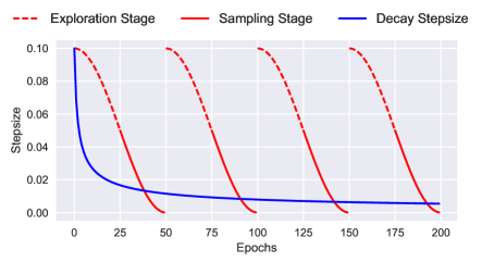
Figure 1: Illustration of the proposed cyclical stepsize schedule (red) and the traditional decreasing stepsize schedule (blue) for SG-MCMC algorithms.

In this paper, we propose to replace the traditional decreasing stepsize schedule in SG-MCMC with a cyclical variant. To note the distinction from traditional SG-MCMC, we refer to this method as Cyclical SG-MCMC (cSG-MCMC). The comparison is illustrated in Figure 1. The blue curve is the traditional decay, while the red curve shows the proposed cyclical schedule. Cyclical SG-MCMC operates in two stages: (i)i(\textup{\it i}) Exploration: when the stepsize is large (dashed red curves), we consider this stage as an effective burn-in mechanism, encouraging the sampler to take large moves and leave the local mode using the stochastic gradient. (ii)ii(\textup{\it ii}) Sampling: when the stepsize is small (solid red curves), the sampler explores one local mode. We collect samples for local distribution estimation during this stage. Further, we propose two practical techniques to improve estimation efficiency: (1) a system temperature for exploration and exploitation; (2) A weighted combination scheme for samples collected in different cycles to reflect their relative importance.

This procedure can be viewed as SG-MCMC with warm restarts: the exploration stage provides the warm restarts for its following sampling stage. cSG-MCMC combines the advantages from (1) the traditional SG-MCMC to characterize the fine-scale local density of a distribution and (2) the cyclical schedule in optimization to efficiently explore multimodal posterior distributions of the parameter space. In limited time, cSG-MCMC is a practical tool to provide significantly better mixing than the traditional SG-MCMC for complex distributions. cSG-MCMC can also be considered as an efficient approximation to parallel MCMC; cSG-MCMC can achieve similar performance to parallel MCMC with only a fraction of cost (reciprocal to the number of chains) that parallel MCMC requires.

To support our proposal, we also prove the non-asymptotic convergence for the cyclical schedule. We note that this is the first convergence analysis of a cyclical stepsize algorithm (including work in optimization). Moreover, we provide extensive experimental results to demonstrate the advantages of cSG-MCMC in sampling from multimodal distributions, including Bayesian neural networks and uncertainty estimation on several large and challenging datasets such as ImageNet.

In short, cSG-MCMC provides a simple and automatic approach to inference in modern Bayesian deep learning, with promising results, and theoretical support. This work is a step towards enabling MCMC approaches in Bayesian deep learning. We release code at
https://github.com/ruqizhang/csgmcmc.

2 Preliminaries: SG-MCMC with a Decreasing Stepsize Schedule

SG-MCMC is a family of scalable sampling methods that enables inference with mini-batches of data. For a dataset 𝒟={di}i=1N𝒟superscriptsubscriptsubscript𝑑𝑖𝑖1𝑁\mathcal{D}=\{d_{i}\}_{i=1}^{N} and a θ𝜃\theta-parameterized model, we have the likelihood p(𝒟|θ)𝑝conditional𝒟𝜃p(\mathcal{D}|\theta) and prior p(θ)𝑝𝜃p(\theta). The posterior distribution is p(θ|𝒟)exp(U(θ)),proportional-to𝑝conditional𝜃𝒟𝑈𝜃p(\theta|\mathcal{D})\propto\exp(-U(\theta))~{}, where U(θ)𝑈𝜃U(\theta) is the potential energy given by U(θ)=logp(𝒟|θ)logp(θ).𝑈𝜃𝑝conditional𝒟𝜃𝑝𝜃U(\theta)=-\log p(\mathcal{D}|\theta)-\log p(\theta)~{}.

When 𝒟𝒟\mathcal{D} is too large, it is expensive to evaluate U(θ)𝑈𝜃U(\theta) for all the data points at each iteration. Instead, SG-MCMC methods use a minibatch to approximate U(θ)𝑈𝜃U(\theta): U~(θ)=NNi=1Nlogp(xi|θ)logp(θ),~𝑈𝜃superscript𝑁𝑁superscriptsubscript𝑖1superscript𝑁𝑝conditionalsubscript𝑥𝑖𝜃𝑝𝜃\tilde{U}(\theta)=-\frac{N^{\prime}}{N}\sum_{i=1}^{N^{\prime}}\log p(x_{i}|\theta)-\log p(\theta)~{}, where NNmuch-less-thansuperscript𝑁𝑁N^{\prime}\ll N is the size of minibatch. We recommend Ma et al. (2015) for a general review of SG-MCMC algorithms. We describe two SG-MCMC algorithms considered in this paper.

SGLD & SGHMC

Welling & Teh (2011) proposed Stochastic Gradient Langevin Dynamics (SGLD), which uses stochastic gradients with Gaussian noise. Posterior samples are updated at the k𝑘k-th step as: θk=θk1αkU~(θk)+2αkϵksubscript𝜃𝑘subscript𝜃𝑘1subscript𝛼𝑘~𝑈subscript𝜃𝑘2subscript𝛼𝑘subscriptitalic-ϵ𝑘\theta_{k}=\theta_{k-1}-\alpha_{k}\nabla\tilde{U}(\theta_{k})+\sqrt{2\alpha_{k}}\epsilon_{k}, where αksubscript𝛼𝑘\alpha_{k} is the stepsize and ϵksubscriptitalic-ϵ𝑘\epsilon_{k} has a standard Gaussian distribution.

To improve mixing over SGLD, Stochastic Gradient Hamiltonian Monte Carlo (SGHMC) (Chen et al., 2014) introduces an auxiliary momentum variable v𝑣v. SGHMC is built upon HMC, with an additional friction term to counteract the noise introduced by a mini-batch. The update rule for posterior samples is: θk=θk1+vk1subscript𝜃𝑘subscript𝜃𝑘1subscript𝑣𝑘1\theta_{k}=\theta_{k-1}+v_{k-1}, and vk=vk1αkU~(θk)ηvk1+2(ηγ^)αkϵksubscript𝑣𝑘subscript𝑣𝑘1subscript𝛼𝑘~𝑈subscript𝜃𝑘𝜂subscript𝑣𝑘12𝜂^𝛾subscript𝛼𝑘subscriptitalic-ϵ𝑘v_{k}=v_{k-1}-\alpha_{k}\nabla\tilde{U}(\theta_{k})-\eta v_{k-1}+\sqrt{2(\eta-\hat{\gamma})\alpha_{k}}\epsilon_{k}, where 1η1𝜂1-\eta is the momentum term and γ^^𝛾\hat{\gamma} is the estimate of the noise.

To guarantee asymptotic consistency with the true distribution, SG-MCMC requires that the step sizes satisfy the following assumption:

Assumption 1.

The step sizes {αk}subscript𝛼𝑘\{\alpha_{k}\} are decreasing, i.e., 0<αk+1<αk0subscript𝛼𝑘1subscript𝛼𝑘0<\alpha_{k+1}<\alpha_{k}, with 1) k=1αk=superscriptsubscript𝑘1subscript𝛼𝑘\sum_{k=1}^{\infty}\alpha_{k}=\infty; and 2) k=1αk2<superscriptsubscript𝑘1superscriptsubscript𝛼𝑘2\sum_{k=1}^{\infty}\alpha_{k}^{2}<\infty.

Without a decreasing step-size, the estimation error from numerical approximations is asymptotically biased. One typical decaying step-size schedule is αk=a(b+k)γsubscript𝛼𝑘𝑎superscript𝑏𝑘𝛾\alpha_{k}=a(b+k)^{-\gamma}, with γ(0.5,1]𝛾0.51\gamma\in(0.5,1] and (a,b)𝑎𝑏(a,b) some positive constants (Welling & Teh, 2011).

3 Cyclical SG-MCMC

We now introduce our cyclical SG-MCMC (cSG-MCMC) algorithm. cSG-MCMC consists of two stages: exploration and sampling. In the following, we first introduce the cyclical step-size schedule, and then describe the exploration stage in Section 3.1 and the sampling stage in Section 3.2. We propose an approach to combining samples for testing in Section F.

Assumption 1 guarantees the consistency of our estimation with the true distribution in the asymptotic time. The approximation error in limited time is characterized as the risk of an estimator R=B2+V𝑅superscript𝐵2𝑉R=B^{2}+V, where B𝐵B is the bias and V𝑉V is the variance. In the case of infinite computation time, the traditional SG-MCMC setting can reduce the bias and variance to zero. However, the time budget is often limited in practice, and there is always a trade-off between bias and variance. We therefore decrease the overall approximation error R𝑅R by reducing the variance through obtaining more effective samples. The effective sample size can be increased if fewer correlated samples from different distribution modes are collected.

For deep neural networks, the parameter space is highly multimodal. In practice, SG-MCMC with the traditional decreasing stepsize schedule becomes trapped in a local mode, though injecting noise may help the sampler to escape in the asymptotic regime (Zhang et al., 2017). Inspired to improve the exploration of the multimodal posteriors for deep neural networks, with a simple and automatic approach, we propose the cyclical cosine stepsize schedule for SG-MCMC. The stepsize at iteration k𝑘k is defined as:

αk=α02[cos(πmod(k1,K/M)K/M)+1],subscript𝛼𝑘subscript𝛼02delimited-[]𝜋mod𝑘1𝐾𝑀𝐾𝑀1\alpha_{k}=\frac{\alpha_{0}}{2}\left[\cos\left(\frac{\pi~{}\text{mod}(k-1,\lceil K/M\rceil)}{\lceil K/M\rceil}\right)+1\right],\vspace{0mm} (1)

where α0subscript𝛼0\alpha_{0} is the initial stepsize, M𝑀M is the number of cycles and K𝐾K is the number of total iterations (Loshchilov & Hutter, 2016; Huang et al., 2017).

The stepsize αksubscript𝛼𝑘\alpha_{k} varies periodically with k𝑘k. In each period, αksubscript𝛼𝑘\alpha_{k} starts at α0subscript𝛼0\alpha_{0}, and gradually decreases to 00. Within one period, SG-MCMC starts with a large stepsize, resulting in aggressive exploration in the parameter space; as the stepsize is decreasing, SG-MCMC explores local regions. In the next period, the Markov chain restarts with a large stepsize, encouraging the sampler to escape from the current mode and explore a new area of the posterior.

Related work in optimization.

In optimization, the cyclical cosine annealing stepsize schedule has been demonstrated to be able to find diverse solutions in multimodal objectives, though not specifically different modes, using stochastic gradient methods (Loshchilov & Hutter, 2016; Huang et al., 2017; Garipov et al., 2018; Fu et al., 2019). Alternatively, we adopt the technique to SG-MCMC as an effective scheme for sampling from multimodal distributions.

3.1 Exploration

The first stage of cyclical SG-MCMC, exploration, discovers parameters near local modes of an objective function. Unfortunately, it is undesirable to directly apply the cyclical schedule in optimization to SG-MCMC for collecting samples at every step. SG-MCMC often requires a small stepsize in order to control the error induced by the noise from using a minibatch approximation. If the stepsize is too large, the stationary distribution of SG-MCMC might be far away from the true posterior distribution. To correct this error, it is possible to do stochastic Metropolis-Hastings (MH) (Korattikara et al., 2014; Bardenet et al., 2014; Chen et al., 2016b). However, stochastic MH correction is still computationally too expensive. Further, it is easy to get rejected with an aggressive large stepsize, and every rejection is a waste of gradient computations.

To alleviate this problem, we propose to introduce a system temperature T𝑇T to control the sampler’s behaviour: p(θ|𝒟)exp(U(θ)/T)proportional-to𝑝conditional𝜃𝒟𝑈𝜃𝑇p(\theta|\mathcal{D})\propto\exp(-U(\theta)/T). Note that the setting T=1𝑇1T=1 corresponds to sampling from the untempered posterior. When T0𝑇0T\rightarrow 0, the posterior distribution becomes a point mass. Sampling from limT0exp(U(θ)/T)subscript𝑇0𝑈𝜃𝑇\lim_{T\rightarrow 0}\exp(-U(\theta)/T) is equivalent to minimizing U(θ)𝑈𝜃U(\theta); in this context, SG-MCMC methods become stochastic gradient optimization methods.

One may increase the temperature T𝑇T from 0 to 1 when the step-size is decreasing. We simply consider T=0𝑇0T=0 and perform optimization as the burn-in stage, when the completed proportion of a cycle r(k)=mod(k1,K/M)K/M𝑟𝑘moduloabsent𝑘1𝐾𝑀𝐾𝑀r(k)=\frac{\mod(k-1,\lceil K/M\rceil)}{\lceil K/M\rceil} is smaller than a given threshold: r(k)<β𝑟𝑘𝛽r(k)<\beta. Note that β(0,1)𝛽01\beta\in(0,1) balances the proportion of the exploration and sampling stages in cSG-MCMC.

Algorithm 1 Cyclical SG-MCMC.
0:  The initial stepsize α0subscript𝛼0\alpha_{0}, number of cycles M𝑀M, number of training iterations K𝐾K and the proportion of exploration stage β𝛽\beta.
  for k = 1:K do
     ααk𝛼subscript𝛼𝑘\alpha\leftarrow\alpha_{k} according to Eq equation 1.
     if mod(k1,K/M)K/M<βmoduloabsent𝑘1𝐾𝑀𝐾𝑀𝛽\frac{\mod(k-1,\lceil K/M\rceil)}{\lceil K/M\rceil}<\beta then
        %𝙴𝚡𝚙𝚕𝚘𝚛𝚊𝚝𝚒𝚘𝚗𝚜𝚝𝚊𝚐𝚎\mathtt{\%~{}Exploration~{}stage}
        θθαU~k(θ)𝜃𝜃𝛼subscript~𝑈𝑘𝜃\theta\leftarrow\theta-\alpha\nabla\tilde{U}_{k}(\theta)
     else
        %𝚂𝚊𝚖𝚙𝚕𝚒𝚗𝚐𝚜𝚝𝚊𝚐𝚎\mathtt{\%~{}Sampling~{}stage}
        Collect samples using SG-MCMC methods
  Samples {θksubscript𝜃𝑘\theta_{k}}

3.2 Sampling

The sampling stage corresponds to T=1𝑇1T=1 of the exploration stage. When r(k)>β𝑟𝑘𝛽r(k)>\beta or step-sizes are sufficiently small, we initiate SG-MCMC updates and collect samples until this cycle ends.

SG-MCMC with Warm Restarts.

One may consider the exploration stage as automatically providing warm restarts for the sampling stage. Exploration alleviates the inefficient mixing and inability to traverse the multimodal distributions of the traditional SG-MCMC methods. SG-MCMC with warm restarts explores different parts of the posterior distribution and captures multiple modes in a single training procedure.

In summary, the proposed cyclical SG-MCMC repeats the two stages, with three key advantages: (i)i(\textup{\it i}) It restarts with a large stepsize at the beginning of a cycle which provides enough perturbation and encourages the model to escape from the current mode. (ii)ii(\textup{\it ii}) The stepsize decreases more quickly inside one cycle than a traditional schedule, making the sampler better characterize the density of the local regions. (iii)iii(\textup{\it iii}) This cyclical stepsize shares the advantage of the “super-convergence” property discussed in Smith & Topin (2017): cSG-MCMC can accelerate convergence for DNNs by up to an order of magnitude.

Connection to the Santa algorithm.

It is interesting to note that our approach inverts steps of the Santa algorithm (Chen et al., 2016a) for optimization. Santa is a simulated-annealing-based optimization algorithm with an exploration stage when T=1𝑇1T=1, then gradually anneals T0𝑇0T\rightarrow 0 in a refinement stage for global optimization. In contrast, our goal is to draw samples for multimodal distributions, thus we explore with T=0𝑇0T=0 and sample with T=1𝑇1T=1. Another fundamental difference is that Santa adopts the traditional stepsize decay, while we use the cyclical schedule.

We visually compare the difference between cyclical and traditional step size schedules (described in Section 2) in Figure 1. The cyclical SG-MCMC algorithm is presented in Algorithm 1.

Connection to Parallel MCMC.

Running parallel Markov chains is a natural and effective way to draw samples from multimodal distributions (VanDerwerken & Schmidler, 2013; Ahn et al., 2014). However, the training cost increases linearly with the number of chains. Cyclical SG-MCMC can be seen as an efficient way to approximate parallel MCMC. Each cycle effectively estimates a different region of posterior. Note cyclical SG-MCMC runs along a single training pass. Therefore, its computational cost is the same as single chain SG-MCMC while significantly less than parallel MCMC.

Combining Samples.

In cyclical SG-MCMC, we obtain samples from multiple modes of a posterior distribution by running the cyclical step size schedule for many periods. We provide a sampling combination scheme to effectively use the collected samples in Section F in the appendix.

4 Theoretical Analysis

Our algorithm is based on the SDE characterizing the Langevin dynamics: dθt=U(θt)dt+2d𝒲tdsubscript𝜃𝑡𝑈subscript𝜃𝑡d𝑡2dsubscript𝒲𝑡\mathrm{d}\theta_{t}=-\nabla U(\theta_{t})\mathrm{d}t+\sqrt{2}\mathrm{d}\mathcal{W}_{t}~{}, where 𝒲tdsubscript𝒲𝑡superscript𝑑\mathcal{W}_{t}\in\mathbb{R}^{d} is a d𝑑d-dimensional Brownian motion. In this section, we prove non-asymptotic convergence rates for the proposed cSG-MCMC framework with a cyclical stepsize sequence {αk}subscript𝛼𝑘\{\alpha_{k}\} defined in equation 1. For simplicity, we do not consider the exploration stage in the analysis as that corresponds to stochastic optimization. Generally, there are two different ways to describe the convergence behaviours of SG-MCMC. One characterizes the sample average over a particular test function (e.g., Chen et al. (2015); Vollmer et al. (2016)); the other is in terms of the Wasserstein distance (e.g., Raginsky et al. (2017); Xu et al. (2017)). We study both in the following.

Weak convergence

Following Chen et al. (2015) and Vollmer et al. (2016), we define the posterior average of an ergodic SDE as: ϕ¯𝒳ϕ(θ)ρ(θ)dθ¯italic-ϕsubscript𝒳italic-ϕ𝜃𝜌𝜃differential-d𝜃\bar{\phi}\triangleq\int_{\mathcal{X}}\phi(\theta)\rho(\theta)\mathrm{d}\theta for some test function ϕ(θ)italic-ϕ𝜃\phi(\theta) of interest. For the corresponding algorithm with generated samples (θk)k=1Ksuperscriptsubscriptsubscript𝜃𝑘𝑘1𝐾(\theta_{k})_{k=1}^{K}, we use the sample average ϕ^^italic-ϕ\hat{\phi} defined as ϕ^=1Kk=1Kϕ(θk)^italic-ϕ1𝐾superscriptsubscript𝑘1𝐾italic-ϕsubscript𝜃𝑘\hat{\phi}=\frac{1}{K}\sum_{k=1}^{K}\phi(\theta_{k}) to approximate ϕ¯¯italic-ϕ\bar{\phi}. We prove weak convergence of cSGLD in terms of bias and MSE, as stated in Theorem 1.

Theorem 1.

Under Assumptions 2 in the appendix, for a smooth test function ϕitalic-ϕ\phi, the bias and MSE of cSGLD are bounded as:

BIAS: |𝔼ϕ~ϕ¯|=O(1α0K+α0),MSE: 𝔼(ϕ~ϕ¯)2=O(1α0K+α02).formulae-sequenceBIAS: 𝔼~italic-ϕ¯italic-ϕ𝑂1subscript𝛼0𝐾subscript𝛼0MSE: 𝔼superscript~italic-ϕ¯italic-ϕ2𝑂1subscript𝛼0𝐾superscriptsubscript𝛼02\displaystyle\text{BIAS: }\left|\mathbb{E}\tilde{\phi}-\bar{\phi}\right|=O\left(\frac{1}{\alpha_{0}K}+\alpha_{0}\right),~{}~{}~{}~{}\text{MSE: }\mathbb{E}\left(\tilde{\phi}-\bar{\phi}\right)^{2}=O\left(\frac{1}{\alpha_{0}K}+\alpha_{0}^{2}\right)~{}. (2)

Convergence under the Wasserstein distance

Next, we consider the more general case of SGLD and characterize convergence rates in terms of a stronger metric of 2-Wasserstein distance, defined as:

W22(μ,ν):=infγ{Ω×Ωθθ22dγ(θ,θ):γΓ(μ,ν)}assignsuperscriptsubscript𝑊22𝜇𝜈subscriptinfimum𝛾conditional-setsubscriptΩΩ:𝜃evaluated-atsuperscript𝜃22d𝛾𝜃superscript𝜃𝛾Γ𝜇𝜈\displaystyle W_{2}^{2}(\mu,\nu):=\inf_{\gamma}\left\{\int_{\Omega\times\Omega}\|\theta-\theta^{\prime}\|_{2}^{2}\mathrm{d}\gamma(\theta,\theta^{\prime}):\gamma\in\Gamma(\mu,\nu)\right\}

where Γ(μ,ν)Γ𝜇𝜈\Gamma(\mu,\nu) is the set of joint distributions over (θ,θ)𝜃superscript𝜃(\theta,\theta^{\prime}) such that the two marginals equal μ𝜇\mu and ν𝜈\nu, respectively.

Denote the distribution of θtsubscript𝜃𝑡\theta_{t} in the SDE as νtsubscript𝜈𝑡\nu_{t}. According to Chiang & Hwang (1987), the stationary distribution νsubscript𝜈\nu_{\infty} matches our target distribution. Let μKsubscript𝜇𝐾\mu_{K} be the distribution of the sample from our proposed cSGLD algorithm at the K𝐾K-th iteration. Our goal is to derive a convergence bound on W2(μK,ν)subscript𝑊2subscript𝜇𝐾subscript𝜈W_{2}(\mu_{K},\nu_{\infty}). We adopt standard assumptions as in most existing work, which are detailed in Assumption 3 in the appendix. Theorem 2 summarizes our main theoretical result.

Theorem 2.

Under Assumption 3 in the appendix, there exist constants (C0,C1,C2,C3)subscript𝐶0subscript𝐶1subscript𝐶2subscript𝐶3(C_{0},C_{1},C_{2},C_{3}) independent of the stepsizes such that the convergence rate of our proposed cSGLD with cyclical stepsize sequence equation 1 is bounded for all K𝐾K satisfying (K𝐾K mod M𝑀M =0), as W2(μK,ν)subscript𝑊2subscript𝜇𝐾subscript𝜈absentW_{2}(\mu_{K},\nu_{\infty})\leq

C3exp(Kα02C4)+(6+C2Kα02)12[(C13α02K8+σC0Kα02)12+(C13α02K16+σC0Kα04)14].subscript𝐶3𝐾subscript𝛼02subscript𝐶4superscript6subscript𝐶2𝐾subscript𝛼0212delimited-[]superscriptsubscript𝐶13superscriptsubscript𝛼02𝐾8𝜎subscript𝐶0𝐾subscript𝛼0212superscriptsubscript𝐶13superscriptsubscript𝛼02𝐾16𝜎subscript𝐶0𝐾subscript𝛼0414\displaystyle C_{3}\exp(-\frac{K\alpha_{0}}{2C_{4}})+\left(6+\frac{C_{2}K\alpha_{0}}{2}\right)^{\frac{1}{2}}[(C_{1}\frac{3\alpha_{0}^{2}K}{8}+\sigma C_{0}\frac{K\alpha_{0}}{2})^{\frac{1}{2}}+(C_{1}\frac{3\alpha_{0}^{2}K}{16}+\sigma C_{0}\frac{K\alpha_{0}}{4})^{\frac{1}{4}}]~{}.

Particularly, if we further assume α0=O(Kβ)subscript𝛼0𝑂superscript𝐾𝛽\alpha_{0}=O(K^{-\beta}) for β>1for-all𝛽1\forall\beta>1, W2(μK,ν)C3+(6+C2Kβ1)12[(2C1K2β1+2C0Kβ1)12+(C1K2β1+C0Kβ1)14]subscript𝑊2subscript𝜇𝐾subscript𝜈subscript𝐶3superscript6subscript𝐶2superscript𝐾𝛽112delimited-[]superscript2subscript𝐶1superscript𝐾2𝛽12subscript𝐶0superscript𝐾𝛽112superscriptsubscript𝐶1superscript𝐾2𝛽1subscript𝐶0superscript𝐾𝛽114W_{2}(\mu_{K},\nu_{\infty})\leq C_{3}+\left(6+\frac{C_{2}}{K^{\beta-1}}\right)^{\frac{1}{2}}[(\frac{2C_{1}}{K^{2\beta-1}}+\frac{2C_{0}}{K^{\beta-1}})^{\frac{1}{2}}+(\frac{C_{1}}{K^{2\beta-1}}+\frac{C_{0}}{K^{\beta-1}})^{\frac{1}{4}}].

Remark 1.

i)\textup{\it i}) The bound is decomposed into two parts: the first part measures convergence speed of exact solution to the stationary distribution, i.e., νkαksubscript𝜈subscript𝑘subscript𝛼𝑘\nu_{\sum_{k}\alpha_{k}} to νsubscript𝜈\nu_{\infty}; the second part measures the numerical error, i.e., between μKsubscript𝜇𝐾\mu_{K} and νkαksubscript𝜈subscript𝑘subscript𝛼𝑘\nu_{\sum_{k}\alpha_{k}}. ii)\textup{\it ii}) The overall bound offers a same order of dependency on K𝐾K as in standard SGLD (please see the bound for SGLD in Section E of the appendix. See also Raginsky et al. (2017)). iii)\textup{\it iii}) If one imposes stricter assumptions such as in the convex case, the bound can be further improved. Specific bounds are derived in the appendix. We did not consider this case due to the discrepancy from real applications.

5 Experiments

We demonstrate cSG-MCMC on several tasks, including a synthetic multimodal distribution (Section 5.1), image classification on Bayesian neural networks (Section 5.2) and uncertainty estimation in Section 5.3. We also demonstrate cSG-MCMC can improve the estimate efficiency for uni-modal distributions using Bayesian logistic regression in Section A.2 in the appendix. We choose SLGD and SGHMC as the representative baseline algorithms. Their cyclical counterpart are called cSGLD and cSGHMC, respectively.

5.1 Synthetic multimodal data
Refer to caption Refer to caption Refer to caption
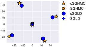
(a) Target (b) SGLD (c) cSGLD
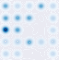
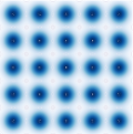
Figure 2: Sampling from a mixture of 25 Gaussians shown in (a) for the parallel setting. With a budget of 50k×4=200k50k4200k50\text{k}\!\times\!4\!=\!\!200\text{k} samples, traditional SGLD in (b) has only discovered 4 of the 25 modes, while our cSGLD in (c) has fully explored the distribution.

We first demonstrate the ability of cSG-MCMC for sampling from a multi-modal distribution on a 2D mixture of 25 Gaussians. Specifically, we compare cSGLD with SGLD in two setting: (1) parallel running with 4 chains and (2) running with a single chain, respectively. Each chain runs for 50k iterations. The stepsize schedule of SGLD is αk0.05k0.55proportional-tosubscript𝛼𝑘0.05superscript𝑘0.55\alpha_{k}\propto 0.05k^{-0.55}. In cSGLD, we set M=30𝑀30M=30 and the initial stepsize α0=0.09subscript𝛼00.09\alpha_{0}=0.09. The proportion of exploration stage β=14𝛽14\beta=\frac{1}{4}. Fig 2 shows the estimated density using sampling results for SGLD and cSGLD in the parallel setting. We observed that SGLD gets trapped in the local modes, depending on the initial position. In any practical time period, SGLD could only characterize partial distribution. In contrast, cSGLD is able to find and characterize all modes, regardless of the initial position. cSGLD leverages large step sizes to discover a new mode, and small step sizes to explore local modes. This result suggests cSGLD can be a significantly favourable choice in the non-asymptotic setting, for example only 50k iterations in this case. The single chain results and the quantitative results on mode coverage are reported in Section A.1 of the appendix.

5.2 Bayesian Neural Networks
Refer to caption Refer to caption Refer to caption
(a) MDS (b) Interpolation (c) Comparison
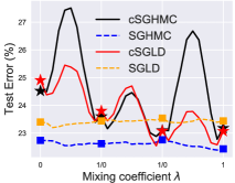
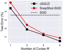
Figure 3: Results of cSG-MCMC with DNNs on the CIFAR-100 dataset. (a) MDS visualization in weight space: cSG-MCMC show larger distance than traditional schedules. (b) Testing errors (%percent\%) on the path of two samples: cSG-MCMC shows more varied performance. (c) Testing errors (%percent\%) as a function of the number of cycles M𝑀M: cSGLD yields consistently lower errors.

We demonstrate the effectiveness of cSG-MCMC on Bayesian neural networks for classification on CIFAR-10 and CIFAR-100. We compare with (i)i(\textup{\it i}) traditional SG-MCMC; (ii)ii(\textup{\it ii}) traditional stochastic optimization methods, including stochastic gradient descent (SGD) and stochastic gradient descent with momentum (SGDM); and (iii)iii(\textup{\it iii}) Snapshot: a stochastic optimization ensemble method method with a the cyclical stepsize schedule  (Huang et al., 2017). We use a ResNet-18 (He et al., 2016) and run all algorithms for 200 epochs. We report the test errors averaged over 3 runs, and the standard error (±plus-or-minus\pm) from the mean predictor.

We set M=4𝑀4M=4 and α0=0.5subscript𝛼00.5\alpha_{0}=0.5 for cSGLD, cSGHMC and Snapshot. The proportion hyper-parameter β=𝛽absent\beta=0.8 and 0.94 for CIFAR-10 and CIFAR-100, respectively. We collect 3 samples per cycle. In practice, we found that the collected samples share similarly high likelihood for DNNs, thus one may simply set the normalizing term wisubscript𝑤𝑖w_{i} in  equation 33 to be the same for faster testing.

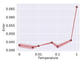
We found that tempering helps improve performance for Bayesian inference with neural networks. Tempering for SG-MCMC was first used by Li et al. (2016a) as a practical technique for neural network training for fast convergence in limited time111https://github.com/ChunyuanLI/pSGLD/issues/2. We simply use the prescribed temperature of Li et al. (2016a) without tuning, but better results of the sampling methods can be achieved by tuning the temperature. More details are in Appendix J. We hypothesize that tempering helps due to the overparametrization of neural networks. Tempering enables one to leverage the inductive biases of the network, while representing the belief that the model capacity can be misspecified. In work on Safe Bayes, also known as generalized and fractional Bayesian inference, tempered posteriors are well-known to help under misspecification (e.g., Barron & Cover, 1991; de Heide et al., 2019; Grünwald et al., 2017).

For the traditional SG-MCMC methods, we found that noise injection early in training hurts convergence. To make these baselines as competitive as possible, we thus avoid noise injection for the first 150 epochs of training (corresponding to the zero temperature limit of SGLD and SGHMC), and resume SGMCMC as usual (with noise) for the last 50 epochs. This scheme is similar to the exploration and sampling stages within one cycle of cSG-MCMC. We collect 20 samples for the MCMC methods and average their predictions in testing.

Testing Performance for Image Classification

We report the testing errors in Table LABEL:tab:CIFAR to compare with the non-parallel algorithms. Snapshot and traditional SG-MCMC reduce the testing errors on both datasets. Performance variance for these methods is also relatively small, due to the multiple networks in the Bayesian model average. Further, cSG-MCMC significantly outperforms Snapshot ensembles and the traditional SG-MCMC, demonstrating the importance of (1) capturing diverse modes compared to traditional SG-MCMC, and (2) capturing fine-scale characteristics of the distribution compared with Snapshot ensembles.

Diversity in Weight Space.

To further demonstrate our hypothesis that with a limited budget cSG-MCMC can find diverse modes, while traditional SG-MCMC cannot, we visualize the 12 samples we collect from cSG-MCMC and SG-MCMC on CIFAR-100 respectively using Multidimensional Scaling (MDS) in Figure 3 (a). MDS uses a Euclidean distance metric between the weight of samples. We see that the samples of cSG-MCMC form 4 clusters, which means they are from 4 different modes in weight space. However, all samples from SG-MCMC only form one cluster, which indicates traditional SG-MCMC gets trapped in one mode and only samples from that mode.

Diversity in Prediction.

To further demonstrate the samples from different cycles of cSG-MCMC provide diverse predictions we choose one sample from each cycle and linearly interpolate between two of them (Goodfellow et al., 2014; Huang et al., 2017). Specifically, let J(θ)𝐽𝜃J(\theta) be the test error of a sample with parameter θ𝜃\theta. We compute the test error of the convex combination of two samples J(λθ1+(1λ)θ2)𝐽𝜆subscript𝜃11𝜆subscript𝜃2J(\lambda\theta_{1}+(1-\lambda)\theta_{2}), where λ[0,1]𝜆01\lambda\in[0,1].

We linearly interpolate between two samples from neighboring chains of cSG-MCMC since they are the most likely to be similar. We randomly select 4 samples from SG-MCMC. If the samples are from the same mode, the test error of the linear interpolation of parameters will be relatively smooth, while if the samples are from different modes, the test error of the parameter interpolation will have a spike when λ𝜆\lambda is between 0 and 1.

We show the results of interpolation for cSG-MCMC and SG-MCMC on CIFAR-100 in Figure 3 (b). We see a spike in the test error in each linear interpolation of parameters between two samples from neighboring chains in cSG-MCMC while the linear interpolation for samples of SG-MCMC is smooth. This result suggests that samples of cSG-MCMC from different chains are from different modes while samples of SG-MCMC are from the same mode.

Although the test error of a single sample of cSG-MCMC is worse than that of SG-MCMC shown in Figure 3 (c), the ensemble of these samples significantly improves the test error, indicating that samples from different modes provide different predictions and make mistakes on different data points. Thus these diverse samples can complement each other, resulting in a lower test error, and demonstrating the advantage of exploring diverse modes using cSG-MCMC.

Table 2: Comparison of test error (%) between cSG-MCMC with parallel algorithm (M𝑀M=4 chains) on CIFAR-10 and CIFAR-100. The method is reported in the format of “step-size schedule (cyclical or decreasing) + single/parallel chain”. The cost is reported in the format of “##\#epoch per chain / ##\#epoch used in all chains”. Note that a parallel algorithm with a single chain reduces to a non-parallel algorithm. Integration of the cyclical schedule with parallel algorithms provides lower testing errors.

Comparison to Parallel MCMC.

cSG-MCMC can be viewed as an economical alternative to parallel MCMC. We verify how closely cSG-MCMC can approximate the performance of parallel MCMC, but with more convenience and less computational expense. We also note that we can improve parallel MCMC with the proposed cyclical stepsize schedule.

We report the testing errors in Table 5.2 to compare multiple-chain results. (1) Four chains used, each runs 200 epochs (800 epochs in total), the results are shown in the first 4 columns (Cyclical+Parallel vs Decreasing+Parallel). We see that cSG-MCMC variants provide lower errors than plain SG-MCMC. (2) We reduce the number of epochs (##\#epoch) of parallel MCMC to 100 epoch each for decreasing stepsize schedule. The total cost is 400 epochs. We compare its performance with cyclical single chain (200 epochs in total) in the last 4 columns (Decreasing+Parallel vs Cyclical+Single). We see that the cyclical schedule running on a single chain performs best even with half the computational cost! All the results indicate the importance of warm re-starts using the proposed cyclical schedule. For a given total cost budget, the proposed cSGMCMC is preferable to parallel sampling.

Comparison to Snapshot Optimization.

We carefully compared with Snapshot, as our cSG-MCMC can be viewed as the sampling counterpart of the Snapshot optimization method. We plot the test error wrt.various number of cycles M𝑀M in Fig. 3. As M𝑀M increases, cSG-MCMC and Snapshot both improve. However, given a fixed M𝑀M, cSG-MCMC yields substantially lower test errors than Snapshot. This result is due to the ability of cSG-MCMC to better characterize the local distribution of modes: Snapshot provides a singe minimum per cycle, while cSG-MCMC fully exploits the mode with more samples, which could provide weight uncertainty estimate and avoid over-fitting.

Results on ImageNet.

We further study different learning algorithms on a large-scale dataset, ImageNet. ResNet-50 is used as the architecture, and 120 epochs for each run. The results on the testing set are summarized in Table LABEL:tab:imagenet, including NLL, Top1 and Top5 accuracy (%percent\%), respectively. 3 cycles are considered for both cSGHMC and Snapshot, and we collect 3 samples per cycle. We see that cSGHMC yields the lowest testing NLL, indicating that the cycle schedule is an effective technique to explore the parameter space, and diversified samples can help prevent over-fitting.

5.3 Uncertainty Evaluation
Refer to caption
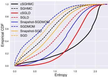
Figure 4: Empirical CDF for the entropy of the predictive distribution on notMNIST dataset. cSGLD and cSGHMC show lower probability for the low entropy estimate than other algorithms.

To demonstrate how predictive uncertainty benefits from exploring multiple modes in the posterior of neural network weights, we consider the task of uncertainty estimation for out-of-distribution samples (Lakshminarayanan et al., 2017). We train a three-layer MLP model on the standard MNIST train dataset until convergence using different algorithms, and estimate the entropy of the predictive distribution on the notMNIST dataset (Bulatov, 2011). Since the samples from the notMNIST dataset belong to the unseen classes, ideally the predictive distribution of the trained model should be uniform over the notMNIST digits, which gives the maximum entropy.

In Figure 4, we plot the empirical CDF for the entropy of the predictive distributions on notMNIST. We see that the uncertainty estimates from cSGHMC and cSGLD are better than the other methods, since the probability of a low entropy prediction is overall lower. cSG-MCMC algorithms explore more modes in the weight space, each mode characterizes a meaningfully different representation of MNIST data. When testing on the out-of-distribution dataset (notMNIST), each mode can provide different predictions over the label space, leading to more reasonable uncertainty estimates. Snapshot achieves less entropy than cSG-MCMC, since it represents each mode with a single point.

The traditional SG-MCMC methods also provide better uncertainty estimation compared to their optimization counterparts, because they characterize a local region of the parameter space, rather than a single point. cSG-MCMC can be regarded as a combination of these two worlds: a wide coverage of many modes in Snapshot, and fine-scale characterization of local regions in SG-MCMC.

6 Discussion

We have proposed cyclical SG-MCMC methods to automatically explore complex multimodal distributions. Our approach is particularly compelling for Bayesian deep learning, which involves rich multimodal parameter posteriors corresponding to meaningfully different representations. We have also shown that our cyclical methods explore unimodal distributions more efficiently. These results are in accordance with theory we developed to show that cyclical SG-MCMC will converge faster to samples from a stationary distribution in general settings. Moreover, we show cyclical SG-MCMC methods provide more accurate uncertainty estimation, by capturing more diversity in the hypothesis space corresponding to settings of model parameters.

While MCMC was once the gold standard for inference with neural networks, it is now rarely used in modern deep learning. We hope that this paper will help renew interest in MCMC for posterior inference in deep learning. Indeed, MCMC is uniquely positioned to explore the rich multimodal posterior distributions of modern neural networks, which can lead to improved accuracy, reliability, and uncertainty representation.

Acknowledgements

AGW was supported by an Amazon Research Award, Facebook Research, NSF I-DISRE 193471, NIH R01 DA048764-01A1, NSF IIS-1563887, and NSF IIS-1910266.

References

  • Ahn et al. (2014) Sungjin Ahn, Babak Shahbaba, and Max Welling. Distributed stochastic gradient MCMC. In ICML, 2014.
  • Auer et al. (1996) Peter Auer, Mark Herbster, and Manfred K Warmuth. Exponentially many local minima for single neurons. In NIPS, 1996.
  • Bardenet et al. (2014) Rémi Bardenet, Arnaud Doucet, and Chris Holmes. Towards scaling up Markov Chain Monte Carlo: an adaptive subsampling approach. In ICML, 2014.
  • Barron & Cover (1991) Andrew R Barron and Thomas M Cover. Minimum complexity density estimation. IEEE transactions on information theory, 37(4):1034–1054, 1991.
  • Blundell et al. (2015) Charles Blundell, Julien Cornebise, Koray Kavukcuoglu, and Daan Wierstra. Weight uncertainty in neural networks. ICML, 2015.
  • Bolley & Villani (2005) François Bolley and Cédric Villani. Weighted csiszár-kullback-pinsker inequalities and applications to transportation inequalities. In Annales de la Faculte des sciences de Toulouse. Université Paul Sabatier, 2005.
  • Bulatov (2011) Yaroslav Bulatov. Not MNIST Dataset. 2011. http://yaroslavvb.blogspot.com/2011/09/notmnist-dataset.html.
  • Chen et al. (2015) Changyou Chen, Nan Ding, and Lawrence Carin. On the convergence of stochastic gradient MCMC algorithms with high-order integrators. In NIPS, 2015.
  • Chen et al. (2016a) Changyou Chen, David Carlson, Zhe Gan, Chunyuan Li, and Lawrence Carin. Bridging the gap between stochastic gradient MCMC and stochastic optimization. In Artificial Intelligence and Statistics, 2016a.
  • Chen et al. (2018) Changyou Chen, Ruiyi Zhang, Wenlin Wang, Bai Li, and Liqun Chen. A unified particle-optimization framework for scalable bayesian sampling. arXiv preprint arXiv:1805.11659, 2018.
  • Chen et al. (2016b) Haoyu Chen, Daniel Seita, Xinlei Pan, and John Canny. An efficient minibatch acceptance test for Metropolis-Hastings. arXiv preprint arXiv:1610.06848, 2016b.
  • Chen et al. (2014) Tianqi Chen, Emily Fox, and Carlos Guestrin. Stochastic gradient Hamiltonian Monte Carlo. In ICML, 2014.
  • Chiang & Hwang (1987) Tzuu-Shuh Chiang and Chii-Ruey Hwang. Diffusion for global optimization in rn. SIAM J. Control Optim., pp.  737–753, 1987. ISSN 0363-0129. doi: 10.1137/0325042. URL http://dx.doi.org/10.1137/0325042.
  • Choromanska et al. (2015) Anna Choromanska, Mikael Henaff, Michael Mathieu, Gérard Ben Arous, and Yann LeCun. The loss surfaces of multilayer networks. In Artificial Intelligence and Statistics, 2015.
  • Dalalyan & Karagulyan (2019) Arnak S. Dalalyan and Avetik Karagulyan. User-friendly guarantees for the langevin monte carlo with inaccurate gradient. Stochastic Processes and their Applications, 2019. ISSN 0304-4149. doi: https://doi.org/10.1016/j.spa.2019.02.016. URL http://www.sciencedirect.com/science/article/pii/S0304414918304824.
  • de Heide et al. (2019) Rianne de Heide, Alisa Kirichenko, Nishant Mehta, and Peter Grünwald. Safe-bayesian generalized linear regression. arXiv preprint arXiv:1910.09227, 2019.
  • Ding et al. (2014) Nan Ding, Youhan Fang, Ryan Babbush, Changyou Chen, Robert D Skeel, and Hartmut Neven. Bayesian sampling using stochastic gradient thermostats. In NIPS, 2014.
  • Fortunato et al. (2017) Meire Fortunato, Charles Blundell, and Oriol Vinyals. Bayesian recurrent neural networks. arXiv preprint arXiv:1704.02798, 2017.
  • Fu et al. (2019) Hao Fu, Chunyuan Li, Xiaodong Liu, Jianfeng Gao, Asli Celikyilmaz, and Lawrence Carin. Cyclical annealing schedule: A simple approach to mitigating KL vanishing. NAACL, 2019.
  • Gan et al. (2016) Zhe Gan, Chunyuan Li, Changyou Chen, Yunchen Pu, Qinliang Su, and Lawrence Carin. Scalable Bayesian learning of recurrent neural networks for language modeling. ACL, 2016.
  • Garipov et al. (2018) Timur Garipov, Pavel Izmailov, Dmitrii Podoprikhin, Dmitry P Vetrov, and Andrew G Wilson. Loss surfaces, mode connectivity, and fast ensembling of DNNs. In Advances in Neural Information Processing Systems, pp. 8789–8798, 2018.
  • Goodfellow et al. (2014) Ian J Goodfellow, Oriol Vinyals, and Andrew M Saxe. Qualitatively characterizing neural network optimization problems. arXiv preprint arXiv:1412.6544, 2014.
  • Green (1995) Peter J Green. Reversible jump MCMC computation and bayesian model determination. Biometrika, 82(4):711–732, 1995.
  • Grünwald et al. (2017) Peter Grünwald, Thijs Van Ommen, et al. Inconsistency of bayesian inference for misspecified linear models, and a proposal for repairing it. Bayesian Analysis, 12(4):1069–1103, 2017.
  • He et al. (2016) Kaiming He, Xiangyu Zhang, Shaoqing Ren, and Jian Sun. Deep residual learning for image recognition. In CVPR, 2016.
  • Hernández-Lobato & Adams (2015) José Miguel Hernández-Lobato and Ryan Adams. Probabilistic backpropagation for scalable learning of Bayesian neural networks. In ICML, 2015.
  • Hoffman & Gelman (2014) Matthew D Hoffman and Andrew Gelman. The no-u-turn sampler: adaptively setting path lengths in hamiltonian monte carlo. Journal of Machine Learning Research, 15(1):1593–1623, 2014.
  • Huang et al. (2017) Gao Huang, Yixuan Li, Geoff Pleiss, Zhuang Liu, John E Hopcroft, and Kilian Q Weinberger. Snapshot ensembles: Train 1, get m for free. ICLR, 2017.
  • Keskar et al. (2016) Nitish Shirish Keskar, Dheevatsa Mudigere, Jorge Nocedal, Mikhail Smelyanskiy, and Ping Tak Peter Tang. On large-batch training for deep learning: Generalization gap and sharp minima. arXiv preprint arXiv:1609.04836, 2016.
  • Korattikara et al. (2014) Anoop Korattikara, Yutian Chen, and Max Welling. Austerity in MCMC land: Cutting the Metropolis-Hastings budget. In ICML, 2014.
  • Lakshminarayanan et al. (2017) Balaji Lakshminarayanan, Alexander Pritzel, and Charles Blundell. Simple and scalable predictive uncertainty estimation using deep ensembles. In NIPS, 2017.
  • Li et al. (2016a) Chunyuan Li, Changyou Chen, David E Carlson, and Lawrence Carin. Preconditioned stochastic gradient Langevin dynamics for deep neural networks. In AAAI, 2016a.
  • Li et al. (2016b) Chunyuan Li, Andrew Stevens, Changyou Chen, Yunchen Pu, Zhe Gan, and Lawrence Carin. Learning weight uncertainty with stochastic gradient MCMC for shape classification. In CVPR, 2016b.
  • Liu et al. (2019) Chang Liu, Jingwei Zhuo, and Jun Zhu. Understanding mcmc dynamics as flows on the wasserstein space. arXiv preprint arXiv:1902.00282, 2019.
  • Loshchilov & Hutter (2016) Ilya Loshchilov and Frank Hutter. Sgdr: Stochastic gradient descent with warm restarts. 2016.
  • Ma et al. (2015) Yi-An Ma, Tianqi Chen, and Emily Fox. A complete recipe for stochastic gradient MCMC. In NIPS, 2015.
  • MacKay (1992) David JC MacKay. A practical bayesian framework for backpropagation networks. Neural computation, 1992.
  • Maddox et al. (2019) Wesley J Maddox, Pavel Izmailov, Timur Garipov, Dmitry P Vetrov, and Andrew Gordon Wilson. A simple baseline for bayesian uncertainty in deep learning. In Advances in Neural Information Processing Systems, pp. 13132–13143, 2019.
  • Mattingly et al. (2010) J. C. Mattingly, A. M. Stuart, and M. V. Tretyakov. Construction of numerical time-average and stationary measures via Poisson equations. SIAM J. NUMER. ANAL., 48(2):552–577, 2010.
  • Neal (1996) Radford M Neal. Bayesian learning for neural networks. New York: Springer-Verlag, 1996.
  • Neelakantan et al. (2016) Arvind Neelakantan, Luke Vilnis, Quoc V Le, Ilya Sutskever, Lukasz Kaiser, Karol Kurach, and James Martens. Adding gradient noise improves learning for very deep networks. ICLR workship, 2016.
  • Nguyen et al. (2017) Anh Nguyen, Jeff Clune, Yoshua Bengio, Alexey Dosovitskiy, and Jason Yosinski. Plug & play generative networks: Conditional iterative generation of images in latent space. In Proceedings of the IEEE Conference on Computer Vision and Pattern Recognition, pp.  4467–4477, 2017.
  • Raftery et al. (2006) Adrian E Raftery, Michael A Newton, Jaya M Satagopan, and Pavel N Krivitsky. Estimating the integrated likelihood via posterior simulation using the harmonic mean identity. 2006.
  • Raginsky et al. (2017) Maxim Raginsky, Alexander Rakhlin, and Matus Telgarsky. Non-convex learning via stochastic gradient Langevin dynamics: a nonasymptotic analysis. arXiv preprint arXiv:1702.03849, 2017.
  • Saatchi & Wilson (2017) Yunus Saatchi and Andrew Gordon Wilson. Bayesian GAN. NIPS, 2017.
  • Santambrogio (2017) Filippo Santambrogio. {Euclidean, metric, and Wasserstein} gradient flows: an overview. Bulletin of Mathematical Sciences, 7(1):87–154, Apr 2017.
  • Smith & Topin (2017) Leslie N Smith and Nicholay Topin. Super-convergence: Very fast training of residual networks using large learning rates. arXiv preprint arXiv:1708.07120, 2017.
  • Teh et al. (2016) Yee Whye Teh, Alexandre H Thiery, and Sebastian J Vollmer. Consistency and fluctuations for stochastic gradient Langevin dynamics. The Journal of Machine Learning Research, 2016.
  • VanDerwerken & Schmidler (2013) Douglas N VanDerwerken and Scott C Schmidler. Parallel Markov Chain Monte Carlo. arXiv preprint arXiv:1312.7479, 2013.
  • Vollmer et al. (2015) S. J. Vollmer, K. C. Zygalakis, and Y. W. Teh. (Non-)asymptotic properties of stochastic gradient Langevin dynamics. Technical Report arXiv:1501.00438, University of Oxford, UK, January 2015. URL http://arxiv.org/abs/1501.00438.
  • Vollmer et al. (2016) Sebastian J. Vollmer, Konstantinos C. Zygalakis, and Yee Whye Teh. Exploration of the (non-)asymptotic bias and variance of stochastic gradient langevin dynamics. Journal of Machine Learning Research, 17(159):1–48, 2016.
  • Welling & Teh (2011) Max Welling and Yee W Teh. Bayesian learning via stochastic gradient Langevin dynamics. In ICML, 2011.
  • Wilson (2020) Andrew Gordon Wilson. The case for bayesian deep learning. arXiv preprint arXiv:2001.10995, 2020.
  • Wilson & Izmailov (2020) Andrew Gordon Wilson and Pavel Izmailov. Bayesian deep learning and a probabilistic perspective of generalization. arXiv preprint arXiv:2002.08791, 2020.
  • Xu et al. (2017) Pan Xu, Jinghui Chen, Difan Zou, and Quanquan Gu. Global convergence of Langevin dynamics based algorithms for nonconvex optimization. arXiv preprint arXiv:1707.06618, 2017.
  • Zhang et al. (2018) Jianyi Zhang, Ruiyi Zhang, and Changyou Chen. Stochastic Particle-Optimization Sampling and the Non-Asymptotic Convergence Theory. arXiv e-prints, art. arXiv:1809.01293, Sep 2018.
  • Zhang et al. (2017) Y. Zhang, P. Liang, and M. Charikar. A hitting time analysis of stochastic gradient Langevin dynamics. In COLT, 2017.

Appendix A Experimental Results

A.1 Synthetic Multimodal Distribution

The density of the distribution is

F(x)=i=125λ𝒩(x|μi,Σ),𝐹𝑥superscriptsubscript𝑖125𝜆𝒩conditional𝑥subscript𝜇𝑖ΣF(x)=\sum_{i=1}^{25}\lambda\mathcal{N}(x|\mu_{i},\Sigma),

where λ=125𝜆125\lambda=\frac{1}{25}, μ={4,2,0,2,4}×{4,2,0,2,4}𝜇superscript42024top42024\mu=\{-4,-2,0,2,4\}^{\top}\times\{-4,-2,0,2,4\}, Σ=[0.03000.03]Σmatrix0.03000.03\Sigma=\begin{bmatrix}0.03&0\\ 0&0.03\end{bmatrix}.

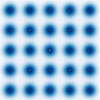
In Figure 5, we show the estimated density for SGLD and cSGLD in the non-parallel setting.
Refer to caption Refer to caption Refer to caption
(a) Target (b) SGLD (c) cSGLD
Figure 5: Sampling from a mixture of 25 Gaussians in the non-parallel setting. With a budget of 50K samples, traditional SGLD has only discovered one of the 25 modes, while our proposed cSGLD has explored significantly more of the distribution.

To quantitatively show the ability of different algorithms to explore multi-modal distributions, we define the mode-coverage metric: when the number of samples falling within the radius r𝑟r of a mode center is larger than a threshold n¯¯𝑛\bar{n}, we consider this mode covered. On this dataset, we choose r=0.25𝑟0.25r=0.25 and n¯=100¯𝑛100\bar{n}=100. Table  4 shows the mode-coverage for several algorithms, based on 10 different runs.

Algorithm Mode coverage
SGLD 1.8±plus-or-minus\pm0.13
cSGLD 6.7±plus-or-minus\pm0.52
Parallel SGLD 18±plus-or-minus\pm0.47
Parallel cSGLD 24.4±plus-or-minus\pm0.22
Table 4: Mode coverage over 10 different runs, ±plus-or-minus\pm standard error.

A.2 Bayesian Logistic Regression

We consider Bayesian logistic regression (BLR) on three real-world datasets from the UCI repository: Australian (15 covariates, 690 data points), German (25 covariates, 1000 data points) and Heart (14 covariates, 270 data points). For all experiments, we collect 5000 samples with 5000 burn-in iterations. Following the settings in Li et al. (2016a), we report median effective sample size (ESS) in Table 5.

Note that BLR is unimodal in parameter space. We use this experiment as an adversarial situation for cSG-MCMC, which we primarily designed to explore multiple modes. We note that even in the unimodal setting, cSG-MCMC more effectively explores the parameter space than popular alternatives. We can also use these experiments to understand how samplers respond to varying parameter dimensionality and training set sizes.

Overall, cSG-MCMC dramatically outperforms SG-MCMC, which demonstrates the fast mixing rate due to the warm restarts. On the small dataset Heart, SGHMC and cSGHMC achieve the same results, because the posterior of BLR on this dataset is simple. However, in higher dimensional spaces (e.g., Australian and German), cSG-MCMC shows significantly higher ESS; this result means that each cycle in cSG-MCMC can characterize a different region of the posteriors, combining multiple cycles yields more accurate overall approximation.

Australian German Heart
SGLD 1676 492 2199
cSGLD 2138 978 2541
SGHMC 1317 2007 5000
cSGHMC 4707 2436 5000
Table 5: Effective sample size for samples for the unimodal posteriors in Bayesian linear regression, obtained using cyclical and traditional SG-MCMC algorithms, respectively.

Appendix B Assumptions

B.1 Assumptions in weak convergence analysis

In the analysis, we define a functional ψ𝜓\psi that solves the following Poisson Equation:

ψ(θk)=ϕ(θk)ϕ¯,or equivalently,1Kk=1Kψ(θk)=ϕ^ϕ¯.formulae-sequence𝜓subscript𝜃𝑘italic-ϕsubscript𝜃𝑘¯italic-ϕor equivalently,1𝐾superscriptsubscript𝑘1𝐾𝜓subscript𝜃𝑘^italic-ϕ¯italic-ϕ\displaystyle\mathcal{L}\psi(\theta_{k})=\phi(\theta_{k})-\bar{\phi},\;\;\text{or equivalently,}\;\;\;\frac{1}{K}\sum_{k=1}^{K}\mathcal{L}\psi(\theta_{k})=\hat{\phi}-\bar{\phi}. (3)

The solution functional ψ(θk)𝜓subscript𝜃𝑘\psi(\theta_{k}) characterizes the difference between ϕ(θk)italic-ϕsubscript𝜃𝑘\phi(\theta_{k}) and the posterior average ϕ¯¯italic-ϕ\bar{\phi} for every θksubscript𝜃𝑘\theta_{k}, thus would typically possess a unique solution, which is at least as smooth as ϕitalic-ϕ\phi under the elliptic or hypoelliptic settings (Mattingly et al., 2010). Following Chen et al. (2015); Vollmer et al. (2016), we make certain assumptions on the solution functional, ψ𝜓\psi, of the Poisson equation equation 3.

Assumption 2.

ψ𝜓\psi and its up to 3rd-order derivatives, 𝒟kψsuperscript𝒟𝑘𝜓\mathcal{D}^{k}\psi, are bounded by a function 𝒱𝒱\mathcal{V}, i.e., 𝒟kψHk𝒱pknormsuperscript𝒟𝑘𝜓subscript𝐻𝑘superscript𝒱subscript𝑝𝑘\|\mathcal{D}^{k}\psi\|\leq H_{k}\mathcal{V}^{p_{k}} for k=(0,1,2,3)𝑘0123k=(0,1,2,3), Hk,pk>0subscript𝐻𝑘subscript𝑝𝑘0H_{k},p_{k}>0. Furthermore, the expectation of 𝒱𝒱\mathcal{V} on {θk}subscript𝜃𝑘\{\theta_{k}\} is bounded: supl𝔼𝒱p(θk)<subscriptsupremum𝑙𝔼superscript𝒱𝑝subscript𝜃𝑘\sup_{l}\mathbb{E}\mathcal{V}^{p}(\theta_{k})<\infty, and 𝒱𝒱\mathcal{V} is smooth such that sups(0,1)𝒱p(sθ+(1s)θ)C(𝒱p(θ)+𝒱p(θ))subscriptsupremum𝑠01superscript𝒱𝑝𝑠𝜃1𝑠superscript𝜃𝐶superscript𝒱𝑝𝜃superscript𝒱𝑝superscript𝜃\sup_{s\in(0,1)}\mathcal{V}^{p}\left(s\theta+\left(1-s\right)\theta^{\prime}\right)\leq C\left(\mathcal{V}^{p}\left(\theta\right)+\mathcal{V}^{p}\left(\theta^{\prime}\right)\right), θ,θ,pmax{2pk}for-all𝜃superscript𝜃𝑝2subscript𝑝𝑘\forall\theta,\theta^{\prime},p\leq\max\{2p_{k}\} for some C>0𝐶0C>0.

B.2 Assumptions in convergence under the Wasserstein distance

Following existing work in Raginsky et al. (2017), we adopt the following standard assumptions summarized in Assumption 3.

Assumption 3.
  • There exists some constants A0𝐴0A\geq 0 and B0𝐵0B\geq 0, such that U(0)A𝑈0𝐴U(0)\leq A and U(0)B𝑈0𝐵\nabla U(0)\leq B.

  • The function U is LUsubscript𝐿𝑈L_{U}-smooth : U(w)U(v)LUwvnorm𝑈𝑤𝑈𝑣subscript𝐿𝑈norm𝑤𝑣\|\nabla U(w)-\nabla U(v)\|\leq L_{U}\|w-v\|.

  • The function U is (mu,b)dissipativesubscript𝑚𝑢𝑏𝑑𝑖𝑠𝑠𝑖𝑝𝑎𝑡𝑖𝑣𝑒(m_{u},b)-dissipative, which means for some mU>0subscript𝑚𝑈0m_{U}>0 and b>0𝑏0b>0 w,U(w)𝑤𝑈𝑤\langle w,\nabla U(w)\rangle \geq mUw2bsubscript𝑚𝑈superscriptnorm𝑤2𝑏m_{U}\|w\|^{2}-b.

  • There exists some constant δ[0,1)𝛿01\delta\in[0,1), such that 𝔼[Uk~(w)U(w)2]2σ(MU2w2+B2)𝔼delimited-[]superscriptnorm~subscript𝑈𝑘𝑤𝑈𝑤22𝜎superscriptsubscript𝑀𝑈2superscriptnorm𝑤2superscript𝐵2\mathbb{E}[\|\nabla\tilde{U_{k}}(w)-\nabla U(w)\|^{2}]\leq 2\sigma(M_{U}^{2}\|w\|^{2}+B^{2}).

  • We can choose μ0subscript𝜇0\mu_{0} which satisfies the requirement: κ0:=logew2μ0(w)𝑑w<assignsubscript𝜅0𝑙𝑜𝑔superscript𝑒superscriptnorm𝑤2subscript𝜇0𝑤differential-d𝑤\kappa_{0}:=log\int e^{\|w\|^{2}}\mu_{0}(w)dw<\infty.

Appendix C Proof of Theorem 1

To prove the theorem, we borrow tools developed by Chen et al. (2015); Vollmer et al. (2015). We first rephrase the stepsize assumptions in general SG-MCMC in Assumption 4.

Assumption 4.

The algorithm adopts an N𝑁N-th order integrator. The step sizes {hk}subscript𝑘\{h_{k}\} are such that 0<hk+1<hk0subscript𝑘1subscript𝑘0<h_{k+1}<h_{k}, and satisfy 1) k=1hk=superscriptsubscript𝑘1subscript𝑘\sum_{k=1}^{\infty}h_{k}=\infty; and 2) limKk=1KhkN+1k=1Khk=0subscript𝐾superscriptsubscript𝑘1𝐾superscriptsubscript𝑘𝑁1superscriptsubscript𝑘1𝐾subscript𝑘0\lim_{K\rightarrow\infty}\frac{\sum_{k=1}^{K}h_{k}^{N+1}}{\sum_{k=1}^{K}h_{k}}=0.

Our prove can be derived by the following results from Chen et al. (2015).

Lemma 1 (Chen et al. (2015)).

Let SKk=1Khksubscript𝑆𝐾superscriptsubscript𝑘1𝐾subscript𝑘S_{K}\triangleq\sum_{k=1}^{K}h_{k}. Under Assumptions 2 and 4, for a smooth test function ϕitalic-ϕ\phi, the bias and MSE of a decreasing-step-size SG-MCMC with a N𝑁Nth-order integrator at time SLsubscript𝑆𝐿S_{L} are bounded as:

BIAS: |𝔼ϕ~ϕ¯|=O(1SK+k=1KhkN+1SK)BIAS: 𝔼~italic-ϕ¯italic-ϕ𝑂1subscript𝑆𝐾superscriptsubscript𝑘1𝐾superscriptsubscript𝑘𝑁1subscript𝑆𝐾\displaystyle\text{BIAS: }\left|\mathbb{E}\tilde{\phi}-\bar{\phi}\right|=O\left(\frac{1}{S_{K}}+\frac{\sum_{k=1}^{K}h_{k}^{N+1}}{S_{K}}\right) (4)
MSE: 𝔼(ϕ~ϕ¯)2C(lhk2SK2𝔼ΔVl2+1SK+(k=1KhkN+1)2SK2).MSE: 𝔼superscript~italic-ϕ¯italic-ϕ2𝐶subscript𝑙superscriptsubscript𝑘2superscriptsubscript𝑆𝐾2𝔼superscriptnormΔsubscript𝑉𝑙21subscript𝑆𝐾superscriptsuperscriptsubscript𝑘1𝐾superscriptsubscript𝑘𝑁12superscriptsubscript𝑆𝐾2\displaystyle\text{MSE: }\mathbb{E}\left(\tilde{\phi}-\bar{\phi}\right)^{2}\leq C\left(\sum_{l}\frac{h_{k}^{2}}{S_{K}^{2}}\mathbb{E}\left\|\Delta V_{l}\right\|^{2}+\frac{1}{S_{K}}+\frac{(\sum_{k=1}^{K}h_{k}^{N+1})^{2}}{S_{K}^{2}}\right)~{}. (5)

Note that Assumption 4 is only required if one wants to prove the asymptotically unbias of an algorithm. Lemma 1 still applies even if Assumption 4 is not satisfied. In this case one would obtain a biased algorithm, which is the case of cSGLD.

Proof of Theorem 1.

Our results is actually a special case of Lemma 1. To see that, first note that our cSGLD adopts a first order integrator, thus N=1𝑁1N=1. To proceed, note that SK=k=1Kαk=O(α0K)subscript𝑆𝐾superscriptsubscript𝑘1𝐾subscript𝛼𝑘𝑂subscript𝛼0𝐾S_{K}=\sum_{k=1}^{K}\alpha_{k}=O(\alpha_{0}K), and

j=0K1αj+12superscriptsubscript𝑗0𝐾1superscriptsubscript𝛼𝑗12\displaystyle\sum_{j=0}^{K-1}\alpha_{j+1}^{2} =α024j=0K1[cos(πmod(j1,[K/M])[K/M])+1]2absentsuperscriptsubscript𝛼024superscriptsubscript𝑗0𝐾1superscriptdelimited-[]𝜋𝑚𝑜𝑑𝑗1delimited-[]𝐾𝑀delimited-[]𝐾𝑀12\displaystyle=\frac{\alpha_{0}^{2}}{4}\sum_{j=0}^{K-1}[\cos(\frac{\pi mod(j-1,[K/M])}{[K/M]})+1]^{2}
=α024j=0K1[cos2(πmod(j1,K/M)K/M)+1]2absentsuperscriptsubscript𝛼024superscriptsubscript𝑗0𝐾1superscriptdelimited-[]superscript2𝜋𝑚𝑜𝑑𝑗1𝐾𝑀𝐾𝑀12\displaystyle=\frac{\alpha_{0}^{2}}{4}\sum_{j=0}^{K-1}[\cos^{2}(\frac{\pi mod(j-1,K/M)}{K/M})+1]^{2}
=α024KM(M2+M)=3α02K8.absentsuperscriptsubscript𝛼024𝐾𝑀𝑀2𝑀3superscriptsubscript𝛼02𝐾8\displaystyle=\frac{\alpha_{0}^{2}}{4}\frac{K}{M}(\frac{M}{2}+M)=\frac{3\alpha_{0}^{2}K}{8}~{}. (6)

As a result, for the bias, we have

|𝔼ϕ~ϕ¯|𝔼~italic-ϕ¯italic-ϕ\displaystyle\left|\mathbb{E}\tilde{\phi}-\bar{\phi}\right| =O(1SK+k=1KhkN+1SK)=O(1α0K+3α02K/8α0K)absent𝑂1subscript𝑆𝐾superscriptsubscript𝑘1𝐾superscriptsubscript𝑘𝑁1subscript𝑆𝐾𝑂1subscript𝛼0𝐾3superscriptsubscript𝛼02𝐾8subscript𝛼0𝐾\displaystyle=O\left(\frac{1}{S_{K}}+\frac{\sum_{k=1}^{K}h_{k}^{N+1}}{S_{K}}\right)=O\left(\frac{1}{\alpha_{0}K}+\frac{3\alpha_{0}^{2}K/8}{\alpha_{0}K}\right)
=O(1α0K+α0).absent𝑂1subscript𝛼0𝐾subscript𝛼0\displaystyle=O\left(\frac{1}{\alpha_{0}K}+\alpha_{0}\right)~{}.

For the MSE, note the first term lhk2SK2𝔼ΔVl2subscript𝑙superscriptsubscript𝑘2superscriptsubscript𝑆𝐾2𝔼superscriptnormΔsubscript𝑉𝑙2\sum_{l}\frac{h_{k}^{2}}{S_{K}^{2}}\mathbb{E}\left\|\Delta V_{l}\right\|^{2} has a higher order than other terms, thus it is omitted in the big-O notation, i.e.,

𝔼(ϕ~ϕ¯)2𝔼superscript~italic-ϕ¯italic-ϕ2\displaystyle\mathbb{E}\left(\tilde{\phi}-\bar{\phi}\right)^{2} =O(1α0K+(3α02K/8α0K)2)absent𝑂1subscript𝛼0𝐾superscript3superscriptsubscript𝛼02𝐾8subscript𝛼0𝐾2\displaystyle=O\left(\frac{1}{\alpha_{0}K}+(\frac{3\alpha_{0}^{2}K/8}{\alpha_{0}K})^{2}\right)
=O(1α0K+α02).absent𝑂1subscript𝛼0𝐾superscriptsubscript𝛼02\displaystyle=O\left(\frac{1}{\alpha_{0}K}+\alpha_{0}^{2}\right)~{}.

This completes the proof. ∎

Appendix D Proof of Theorem 2

Proof of the bound for W2(μK,ν)subscript𝑊2subscript𝜇𝐾subscript𝜈W_{2}(\mu_{K},\nu_{\infty}) in cSGLD.

Firstly, we introduce the following SDE

dθt=U(θt)dt+2d𝒲t,dsubscript𝜃𝑡𝑈subscript𝜃𝑡d𝑡2dsubscript𝒲𝑡\displaystyle\mathrm{d}\theta_{t}=-\nabla U(\theta_{t})\mathrm{d}t+\sqrt{2}\mathrm{d}\mathcal{W}_{t}~{}, (7)

Let νtsubscript𝜈𝑡\nu_{t} denote the distribution of θtsubscript𝜃𝑡\theta_{t}, and the stationary distribution of equation 34 be p(θ|𝒟)𝑝conditional𝜃𝒟p(\theta|\mathcal{D}), which means ν=p(θ|𝒟)subscript𝜈𝑝conditional𝜃𝒟\nu_{\infty}=p(\theta|\mathcal{D}).

θk+1=θkUk~(θk)αk+1+2αk+1ξk+1subscript𝜃𝑘1subscript𝜃𝑘~subscript𝑈𝑘subscript𝜃𝑘subscript𝛼𝑘12subscript𝛼𝑘1subscript𝜉𝑘1\displaystyle\theta_{k+1}=\theta_{k}-\nabla\tilde{U_{k}}(\theta_{k})\alpha_{k+1}+\sqrt{2\alpha_{k+1}}\xi_{k+1} (8)

Further, let μksubscript𝜇𝑘\mu_{k} denote the distribution of θksubscript𝜃𝑘\theta_{k}.

Since

W2(μK,ν)W2(μK,νk=1Kαk)+W2(νk=1Kαk,ν)subscript𝑊2subscript𝜇𝐾subscript𝜈subscript𝑊2subscript𝜇𝐾subscript𝜈superscriptsubscript𝑘1𝐾subscript𝛼𝑘subscript𝑊2subscript𝜈superscriptsubscript𝑘1𝐾subscript𝛼𝑘subscript𝜈\displaystyle W_{2}(\mu_{K},\nu_{\infty})\leq W_{2}(\mu_{K},\nu_{\sum_{k=1}^{K}\alpha_{k}})+W_{2}(\nu_{\sum_{k=1}^{K}\alpha_{k}},\nu_{\infty}) (9)

, we need to give the bounds for these two parts respectively.

D.1 W2(μK,νk=1Kαk)subscript𝑊2subscript𝜇𝐾subscript𝜈superscriptsubscript𝑘1𝐾subscript𝛼𝑘W_{2}(\mu_{K},\nu_{\sum_{k=1}^{K}\alpha_{k}})

For the first part, W2(μK,νk=1Kαk)subscript𝑊2subscript𝜇𝐾subscript𝜈superscriptsubscript𝑘1𝐾subscript𝛼𝑘W_{2}(\mu_{K},\nu_{\sum_{k=1}^{K}\alpha_{k}}), our proof is based on the proof of Lemma 3.6 in Raginsky et al. (2017) with some modifications. We first assume 𝔼(U~(w))=U(w),wd,formulae-sequence𝔼~𝑈𝑤𝑈𝑤for-all𝑤superscript𝑑\mathbb{E}(\nabla\tilde{U}(w))=\nabla{U}(w),~{}~{}\forall w\in\mathbb{R}^{d}~{}, which is a general assumption according to the way we choose the minibatch. And we define p(t)𝑝𝑡p(t) which will be used in the following proof:

p(t)={k|i=1kαit<i=1k+1αi}𝑝𝑡conditional-set𝑘superscriptsubscript𝑖1𝑘subscript𝛼𝑖𝑡superscriptsubscript𝑖1𝑘1subscript𝛼𝑖\displaystyle p(t)=\{k\in\mathbb{Z}|\sum_{i=1}^{k}\alpha_{i}\leq t<\sum_{i=1}^{k+1}\alpha_{i}\} (10)

Then we focus on the following continuous-time interpolation of θksubscript𝜃𝑘\theta_{k}:

θ¯(t)=¯𝜃𝑡absent\displaystyle\underline{\theta}(t)= θ00tU~(θ¯(k=1p(s)αk))ds+20t𝑑𝒲s(d)subscript𝜃0superscriptsubscript0𝑡~𝑈¯𝜃superscriptsubscript𝑘1𝑝𝑠subscript𝛼𝑘differential-d𝑠2superscriptsubscript0𝑡differential-dsuperscriptsubscript𝒲𝑠𝑑\displaystyle{\theta}_{0}-\int_{0}^{t}\nabla\tilde{U}\left(\underline{\theta}(\sum_{k=1}^{p(s)}\alpha_{k})\right)\mathrm{d}s+\sqrt{2}\int_{0}^{t}d\mathcal{W}_{s}^{(d)} (11)

where U~U~k~𝑈subscript~𝑈𝑘\nabla\tilde{U}\equiv\nabla\tilde{U}_{k} for t[i=1kαi,i=1k+1αi)𝑡superscriptsubscript𝑖1𝑘subscript𝛼𝑖superscriptsubscript𝑖1𝑘1subscript𝛼𝑖t\in\left[\sum_{i=1}^{k}\alpha_{i},\sum_{i=1}^{k+1}\alpha_{i}\right). And for each k , θ¯(i=1kαi)¯𝜃superscriptsubscript𝑖1𝑘subscript𝛼𝑖\underline{{\theta}}(\sum_{i=1}^{k}\alpha_{i}) and θksubscript𝜃𝑘{\theta}_{k} have the same probability law μksubscript𝜇𝑘\mu_{k}.
Since θ¯(t)¯𝜃𝑡\underline{\theta}(t) is not a Markov process, we define the following process which has the same one-time marginals as θ¯(t)¯𝜃𝑡\underline{\theta}(t)

V(t)=θ00tGs(V(s))ds+20t𝑑𝒲s(d)𝑉𝑡subscript𝜃0superscriptsubscript0𝑡subscript𝐺𝑠𝑉𝑠differential-d𝑠2superscriptsubscript0𝑡differential-dsuperscriptsubscript𝒲𝑠𝑑\displaystyle V(t)={\theta}_{0}-\int_{0}^{t}{G}_{s}\left(V(s)\right)\mathrm{d}s+\sqrt{2}\int_{0}^{t}d\mathcal{W}_{s}^{(d)} (12)

with

Gt(x):=𝔼[U~(θ¯(i=1q(t)αi))|θ¯(t)=x]assignsubscript𝐺𝑡𝑥𝔼delimited-[]conditional~𝑈¯𝜃superscriptsubscript𝑖1𝑞𝑡subscript𝛼𝑖¯𝜃𝑡𝑥\displaystyle G_{t}(x):=\mathbb{E}\left[\nabla\tilde{U}\left(\underline{\theta}(\sum_{i=1}^{q(t)}\alpha_{i})\right)|\underline{\theta}(t)=x\right] (13)

Let 𝐏Vt:=(V(s):0st)\operatorname{\mathbf{P}}_{V}^{t}:=\mathcal{L}\left(V(s):0\leq s\leq t\right) and 𝐏θt:=(θ(s):0st)\operatorname{\mathbf{P}}_{\theta}^{t}:=\mathcal{L}\left(\theta(s):0\leq s\leq t\right) and according to the proof of Lemma 3.6 in Raginsky et al. (2017), we can derive a similar result for the relative entropy of 𝐏Vtsuperscriptsubscript𝐏𝑉𝑡\operatorname{\mathbf{P}}_{V}^{t} and 𝐏θtsuperscriptsubscript𝐏𝜃𝑡\operatorname{\mathbf{P}}_{\theta}^{t}:

DKL(𝐏Vt𝐏θt)=subscript𝐷𝐾𝐿conditionalsuperscriptsubscript𝐏𝑉𝑡superscriptsubscript𝐏𝜃𝑡absent\displaystyle D_{KL}(\operatorname{\mathbf{P}}_{V}^{t}\|\operatorname{\mathbf{P}}_{\theta}^{t})= d𝐏Vtlogd𝐏Vtd𝐏θtdsuperscriptsubscript𝐏𝑉𝑡logdsuperscriptsubscript𝐏𝑉𝑡dsuperscriptsubscript𝐏𝜃𝑡\displaystyle-\int\mathrm{d}\operatorname{\mathbf{P}}_{V}^{t}\text{log}\frac{\mathrm{d}\operatorname{\mathbf{P}}_{V}^{t}}{\mathrm{d}\operatorname{\mathbf{P}}_{\theta}^{t}}
=140t𝔼U(V(s))Gs(V(s))2dsabsent14superscriptsubscript0𝑡𝔼superscriptnorm𝑈𝑉𝑠subscript𝐺𝑠𝑉𝑠2differential-d𝑠\displaystyle=\frac{1}{4}\int_{0}^{t}\mathbb{E}\|\nabla U(V(s))-G_{s}(V(s))\|^{2}\mathrm{d}s
=140t𝔼U(θ¯(s))Gs(θ¯(s))2dsabsent14superscriptsubscript0𝑡𝔼superscriptnorm𝑈¯𝜃𝑠subscript𝐺𝑠¯𝜃𝑠2differential-d𝑠\displaystyle=\frac{1}{4}\int_{0}^{t}\mathbb{E}\|\nabla U(\underline{\theta}(s))-G_{s}(\underline{\theta}(s))\|^{2}\mathrm{d}s

The last line follows the fact that (θ¯(s))=(V(s)),s¯𝜃𝑠𝑉𝑠for-all𝑠\mathcal{L}(\underline{\theta}(s))=\mathcal{L}(V(s)),~{}\forall s.
Then we will let t=k=1Kαk𝑡superscriptsubscript𝑘1𝐾subscript𝛼𝑘t=\sum_{k=1}^{K}\alpha_{k} and we can use the martingale property of the integral to derive:

DKL(𝐏Vk=1Kαk𝐏θk=1Kαk)subscript𝐷𝐾𝐿conditionalsuperscriptsubscript𝐏𝑉superscriptsubscript𝑘1𝐾subscript𝛼𝑘superscriptsubscript𝐏𝜃superscriptsubscript𝑘1𝐾subscript𝛼𝑘\displaystyle D_{KL}(\operatorname{\mathbf{P}}_{V}^{\sum_{k=1}^{K}\alpha_{k}}\|\operatorname{\mathbf{P}}_{\theta}^{\sum_{k=1}^{K}\alpha_{k}})
=14j=0K1k=1jαkk=1j+1αk𝔼U(θ¯(s))Gs(θ¯(s))2dsabsent14superscriptsubscript𝑗0𝐾1superscriptsubscriptsuperscriptsubscript𝑘1𝑗subscript𝛼𝑘superscriptsubscript𝑘1𝑗1subscript𝛼𝑘𝔼superscriptnorm𝑈¯𝜃𝑠subscript𝐺𝑠¯𝜃𝑠2differential-d𝑠\displaystyle=\frac{1}{4}\sum_{j=0}^{K-1}\int_{\sum_{k=1}^{j}\alpha_{k}}^{\sum_{k=1}^{j+1}\alpha_{k}}\mathbb{E}\|\nabla U(\underline{\theta}(s))-G_{s}(\underline{\theta}(s))\|^{2}\mathrm{d}s
12j=0K1k=1jαkk=1j+1αk𝔼U(θ¯(s))U(θ¯(k=1q(s)αi)2ds\displaystyle\leq\frac{1}{2}\sum_{j=0}^{K-1}\int_{\sum_{k=1}^{j}\alpha_{k}}^{\sum_{k=1}^{j+1}\alpha_{k}}\mathbb{E}\|\nabla U(\underline{\theta}(s))-\nabla U(\underline{\theta}(\sum_{k=1}^{q(s)}\alpha_{i})\|^{2}\mathrm{d}s
+12j=0K1k=1jαkk=1j+1αk𝔼U(θ¯(k=1q(s)αi)Gs(θ¯(k=1q(s)αi)2ds\displaystyle\hskip 20.00003pt+\frac{1}{2}\sum_{j=0}^{K-1}\int_{\sum_{k=1}^{j}\alpha_{k}}^{\sum_{k=1}^{j+1}\alpha_{k}}\mathbb{E}\|\nabla U(\underline{\theta}(\sum_{k=1}^{q(s)}\alpha_{i})-G_{s}(\underline{\theta}(\sum_{k=1}^{q(s)}\alpha_{i})\|^{2}\mathrm{d}s
LU22j=0K1k=1jαkk=1j+1αk𝔼θ¯(s)θ¯(k=1q(s)αi)2dsabsentsuperscriptsubscript𝐿𝑈22superscriptsubscript𝑗0𝐾1superscriptsubscriptsuperscriptsubscript𝑘1𝑗subscript𝛼𝑘superscriptsubscript𝑘1𝑗1subscript𝛼𝑘𝔼superscriptnorm¯𝜃𝑠¯𝜃superscriptsubscript𝑘1𝑞𝑠subscript𝛼𝑖2differential-d𝑠\displaystyle\leq\frac{L_{U}^{2}}{2}\sum_{j=0}^{K-1}\int_{\sum_{k=1}^{j}\alpha_{k}}^{\sum_{k=1}^{j+1}\alpha_{k}}\mathbb{E}\|\underline{\theta}(s)-\underline{\theta}(\sum_{k=1}^{q(s)}\alpha_{i})\|^{2}\mathrm{d}s (14)
+12j=0K1k=1jαkk=1j+1αk𝔼U(θ¯(k=1q(s)αi)Gs(θ¯(k=1q(s)αi)2ds\displaystyle\hskip 20.00003pt+\frac{1}{2}\sum_{j=0}^{K-1}\int_{\sum_{k=1}^{j}\alpha_{k}}^{\sum_{k=1}^{j+1}\alpha_{k}}\mathbb{E}\|\nabla U(\underline{\theta}(\sum_{k=1}^{q(s)}\alpha_{i})-G_{s}(\underline{\theta}(\sum_{k=1}^{q(s)}\alpha_{i})\|^{2}\mathrm{d}s (15)

For the first part (14), we consider some s[k=1jαk,k=1j+1αk)𝑠superscriptsubscript𝑘1𝑗subscript𝛼𝑘superscriptsubscript𝑘1𝑗1subscript𝛼𝑘s\in[{\sum_{k=1}^{j}\alpha_{k}},{\sum_{k=1}^{j+1}\alpha_{k}}), for which the following holds:

θ¯(s)θ¯(k=1jαk)¯𝜃𝑠¯𝜃superscriptsubscript𝑘1𝑗subscript𝛼𝑘\displaystyle\underline{\theta}(s)-\underline{\theta}(\sum_{k=1}^{j}\alpha_{k})
=(sk=1jαk)U~k(θk)+2(𝒲s(d)𝒲k=1jαk(d))absent𝑠superscriptsubscript𝑘1𝑗subscript𝛼𝑘subscript~𝑈𝑘subscript𝜃𝑘2superscriptsubscript𝒲𝑠𝑑superscriptsubscript𝒲superscriptsubscript𝑘1𝑗subscript𝛼𝑘𝑑\displaystyle=-(s-\sum_{k=1}^{j}\alpha_{k})\nabla\tilde{U}_{k}(\theta_{k})+\sqrt{2}(\mathcal{W}_{s}^{(d)}-\mathcal{W}_{\sum_{k=1}^{j}\alpha_{k}}^{(d)})
=(sk=1jαk)U(θk)+(sk=1jαk)(U(θk)U~k(θk))+2(𝒲s(d)𝒲k=1jαk(d))absent𝑠superscriptsubscript𝑘1𝑗subscript𝛼𝑘𝑈subscript𝜃𝑘𝑠superscriptsubscript𝑘1𝑗subscript𝛼𝑘𝑈subscript𝜃𝑘subscript~𝑈𝑘subscript𝜃𝑘2superscriptsubscript𝒲𝑠𝑑superscriptsubscript𝒲superscriptsubscript𝑘1𝑗subscript𝛼𝑘𝑑\displaystyle=-(s-\sum_{k=1}^{j}\alpha_{k})\nabla U(\theta_{k})+(s-\sum_{k=1}^{j}\alpha_{k})(\nabla U(\theta_{k})-\nabla\tilde{U}_{k}(\theta_{k}))+\sqrt{2}(\mathcal{W}_{s}^{(d)}-\mathcal{W}_{\sum_{k=1}^{j}\alpha_{k}}^{(d)}) (16)

Thus, we can use Lemma 3.1 and 3.2 in Raginsky et al. (2017) for the following result:

𝔼θ¯(s)θ¯(k=1jαk)2𝔼superscriptnorm¯𝜃𝑠¯𝜃superscriptsubscript𝑘1𝑗subscript𝛼𝑘2\displaystyle\mathbb{E}\|\underline{\theta}(s)-\underline{\theta}(\sum_{k=1}^{j}\alpha_{k})\|^{2} 3αj+12𝔼U(θj)2+3αj+12𝔼U(θj)U~j(θj)2+6αj+1dabsent3superscriptsubscript𝛼𝑗12𝔼superscriptnorm𝑈subscript𝜃𝑗23superscriptsubscript𝛼𝑗12𝔼superscriptnorm𝑈subscript𝜃𝑗subscript~𝑈𝑗subscript𝜃𝑗26subscript𝛼𝑗1𝑑\displaystyle\leq 3\alpha_{j+1}^{2}\mathbb{E}\|\nabla U(\theta_{j})\|^{2}+3\alpha_{j+1}^{2}\mathbb{E}\|\nabla U(\theta_{j})-\nabla\tilde{U}_{j}(\theta_{j})\|^{2}+6\alpha_{j+1}d
12αj+12(LU2𝔼θj2+B2)+6αj+1dabsent12superscriptsubscript𝛼𝑗12superscriptsubscript𝐿𝑈2𝔼superscriptnormsubscript𝜃𝑗2superscript𝐵26subscript𝛼𝑗1𝑑\displaystyle\leq 12\alpha_{j+1}^{2}(L_{U}^{2}\mathbb{E}\|\theta_{j}\|^{2}+B^{2})+6\alpha_{j+1}d

Hence we can bound the first part, (choosing α01subscript𝛼01\alpha_{0}\leq 1),

LU22j=0K1k=1jαkk=1j+1αk𝔼θ¯(s)θ¯(k=1q(s)αi)2dssuperscriptsubscript𝐿𝑈22superscriptsubscript𝑗0𝐾1superscriptsubscriptsuperscriptsubscript𝑘1𝑗subscript𝛼𝑘superscriptsubscript𝑘1𝑗1subscript𝛼𝑘𝔼superscriptnorm¯𝜃𝑠¯𝜃superscriptsubscript𝑘1𝑞𝑠subscript𝛼𝑖2differential-d𝑠\displaystyle\frac{L_{U}^{2}}{2}\sum_{j=0}^{K-1}\int_{\sum_{k=1}^{j}\alpha_{k}}^{\sum_{k=1}^{j+1}\alpha_{k}}\mathbb{E}\|\underline{\theta}(s)-\underline{\theta}(\sum_{k=1}^{q(s)}\alpha_{i})\|^{2}\mathrm{d}s
LU22j=0K1[12αj+13(LU2𝔼θj2+B2)+6αj+12d]absentsuperscriptsubscript𝐿𝑈22superscriptsubscript𝑗0𝐾1delimited-[]12superscriptsubscript𝛼𝑗13superscriptsubscript𝐿𝑈2𝔼superscriptnormsubscript𝜃𝑗2superscript𝐵26superscriptsubscript𝛼𝑗12𝑑\displaystyle\leq\frac{L_{U}^{2}}{2}\sum_{j=0}^{K-1}\left[12\alpha_{j+1}^{3}(L_{U}^{2}\mathbb{E}\|\theta_{j}\|^{2}+B^{2})+6\alpha_{j+1}^{2}d\right]
LU2max0jK1[6(LU2𝔼θj2+B2)+3d](j=0K1αj+12)absentsuperscriptsubscript𝐿𝑈2subscript0𝑗𝐾16superscriptsubscript𝐿𝑈2𝔼superscriptnormsubscript𝜃𝑗2superscript𝐵23𝑑superscriptsubscript𝑗0𝐾1superscriptsubscript𝛼𝑗12\displaystyle\leq{L_{U}^{2}}\max_{0\leq j\leq K-1}\left[6(L_{U}^{2}\mathbb{E}\|\theta_{j}\|^{2}+B^{2})+3d\right](\sum_{j=0}^{K-1}\alpha_{j+1}^{2})
LU2max0jK1[6(LU2𝔼θj2+B2)+3d]3α02K8absentsuperscriptsubscript𝐿𝑈2subscript0𝑗𝐾16superscriptsubscript𝐿𝑈2𝔼superscriptnormsubscript𝜃𝑗2superscript𝐵23𝑑3superscriptsubscript𝛼02𝐾8\displaystyle\leq{L_{U}^{2}}\max_{0\leq j\leq K-1}\left[6(L_{U}^{2}\mathbb{E}\|\theta_{j}\|^{2}+B^{2})+3d\right]\frac{3\alpha_{0}^{2}K}{8} (17)

The last line (17) follows from222Note: we only focus on the case when KmodM=0modulo𝐾𝑀0K\mod M=0. equation C. The second part (15) can be bounded as follows:

12j=0K1k=1jαkk=1j+1αk𝔼U(θ¯(k=1q(s)αi)Gs(θ¯(k=1q(s)αi)2ds\displaystyle\frac{1}{2}\sum_{j=0}^{K-1}\int_{\sum_{k=1}^{j}\alpha_{k}}^{\sum_{k=1}^{j+1}\alpha_{k}}\mathbb{E}\|\nabla U(\underline{\theta}(\sum_{k=1}^{q(s)}\alpha_{i})-G_{s}(\underline{\theta}(\sum_{k=1}^{q(s)}\alpha_{i})\|^{2}\mathrm{d}s
=12j=0K1αj+1𝔼U(θj)U~(θj)2absent12superscriptsubscript𝑗0𝐾1subscript𝛼𝑗1𝔼superscriptnorm𝑈subscript𝜃𝑗~𝑈subscript𝜃𝑗2\displaystyle=\frac{1}{2}\sum_{j=0}^{K-1}\alpha_{j+1}\mathbb{E}\|\nabla U({\theta}_{j})-\nabla\tilde{U}({\theta}_{j})\|^{2}
σmax0jK1(LU2𝔼θj2+B2)j=0K1αj+1absent𝜎subscript0𝑗𝐾1superscriptsubscript𝐿𝑈2𝔼superscriptnormsubscript𝜃𝑗2superscript𝐵2superscriptsubscript𝑗0𝐾1subscript𝛼𝑗1\displaystyle\leq\sigma\max_{0\leq j\leq K-1}(L_{U}^{2}\mathbb{E}\|\theta_{j}\|^{2}+B^{2})\sum_{j=0}^{K-1}\alpha_{j+1}
σmax0jK1(LU2𝔼θj2+B2)(α02j=0K1(cos(πmod(j,K/M)K/M)+1))absent𝜎subscript0𝑗𝐾1superscriptsubscript𝐿𝑈2𝔼superscriptnormsubscript𝜃𝑗2superscript𝐵2subscript𝛼02superscriptsubscript𝑗0𝐾1𝜋𝑚𝑜𝑑𝑗𝐾𝑀𝐾𝑀1\displaystyle\leq\sigma\max_{0\leq j\leq K-1}(L_{U}^{2}\mathbb{E}\|\theta_{j}\|^{2}+B^{2})(\frac{\alpha_{0}}{2}\sum_{j=0}^{K-1}(\cos(\frac{\pi mod(j,K/M)}{K/M})+1))
σmax0jK1(LU2𝔼θj2+B2)(Kα02)absent𝜎subscript0𝑗𝐾1superscriptsubscript𝐿𝑈2𝔼superscriptnormsubscript𝜃𝑗2superscript𝐵2𝐾subscript𝛼02\displaystyle\leq\sigma\max_{0\leq j\leq K-1}(L_{U}^{2}\mathbb{E}\|\theta_{j}\|^{2}+B^{2})(\frac{K\alpha_{0}}{2})

Due to the data-processing inequality for the relative entropy, we have

DKL(μKνk=1Kαk)DKL(𝐏Vt𝐏θt)subscript𝐷𝐾𝐿conditionalsubscript𝜇𝐾subscript𝜈superscriptsubscript𝑘1𝐾subscript𝛼𝑘subscript𝐷𝐾𝐿conditionalsuperscriptsubscript𝐏𝑉𝑡superscriptsubscript𝐏𝜃𝑡\displaystyle D_{KL}(\mu_{K}\|\nu_{\sum_{k=1}^{K}\alpha_{k}})\leq D_{KL}(\operatorname{\mathbf{P}}_{V}^{t}\|\operatorname{\mathbf{P}}_{\theta}^{t})
LU22j=0K1k=1jαkk=1j+1αk𝔼θ¯(s)θ¯(k=1q(s)αi)2dsabsentsuperscriptsubscript𝐿𝑈22superscriptsubscript𝑗0𝐾1superscriptsubscriptsuperscriptsubscript𝑘1𝑗subscript𝛼𝑘superscriptsubscript𝑘1𝑗1subscript𝛼𝑘𝔼superscriptnorm¯𝜃𝑠¯𝜃superscriptsubscript𝑘1𝑞𝑠subscript𝛼𝑖2differential-d𝑠\displaystyle\leq\frac{L_{U}^{2}}{2}\sum_{j=0}^{K-1}\int_{\sum_{k=1}^{j}\alpha_{k}}^{\sum_{k=1}^{j+1}\alpha_{k}}\mathbb{E}\|\underline{\theta}(s)-\underline{\theta}(\sum_{k=1}^{q(s)}\alpha_{i})\|^{2}\mathrm{d}s
+12j=0K1k=1jαkk=1j+1αk𝔼U(θ¯(k=1q(s)αi)Gs(θ¯(k=1q(s)αi)2ds\displaystyle\hskip 20.00003pt+\frac{1}{2}\sum_{j=0}^{K-1}\int_{\sum_{k=1}^{j}\alpha_{k}}^{\sum_{k=1}^{j+1}\alpha_{k}}\mathbb{E}\|\nabla U(\underline{\theta}(\sum_{k=1}^{q(s)}\alpha_{i})-G_{s}(\underline{\theta}(\sum_{k=1}^{q(s)}\alpha_{i})\|^{2}\mathrm{d}s
LU2max0jK1[6(LU2𝔼θj2+B2)+3d]3α02K8absentsuperscriptsubscript𝐿𝑈2subscript0𝑗𝐾16superscriptsubscript𝐿𝑈2𝔼superscriptnormsubscript𝜃𝑗2superscript𝐵23𝑑3superscriptsubscript𝛼02𝐾8\displaystyle\leq{L_{U}^{2}}\max_{0\leq j\leq K-1}\left[6(L_{U}^{2}\mathbb{E}\|\theta_{j}\|^{2}+B^{2})+3d\right]\frac{3\alpha_{0}^{2}K}{8}
+σmax0jK1(LU2𝔼θj2+B2)(Kα02)𝜎subscript0𝑗𝐾1superscriptsubscript𝐿𝑈2𝔼superscriptnormsubscript𝜃𝑗2superscript𝐵2𝐾subscript𝛼02\displaystyle\hskip 20.00003pt+\sigma\max_{0\leq j\leq K-1}(L_{U}^{2}\mathbb{E}\|\theta_{j}\|^{2}+B^{2})(\frac{K\alpha_{0}}{2})

According to the proof of Lemma 3.2 in Raginsky et al. (2017), we can bound the term 𝔼θk2𝔼superscriptnormsubscript𝜃𝑘2\mathbb{E}\|\theta_{k}\|^{2}

𝔼θk+12(12αk+1mU+4αk+12MU2)𝔼θk2+2αk+1b+4αk+12B2+2αk+1dβ𝔼superscriptnormsubscript𝜃𝑘1212subscript𝛼𝑘1subscript𝑚𝑈4superscriptsubscript𝛼𝑘12superscriptsubscript𝑀𝑈2𝔼superscriptnormsubscript𝜃𝑘22subscript𝛼𝑘1𝑏4superscriptsubscript𝛼𝑘12superscript𝐵22subscript𝛼𝑘1𝑑𝛽\displaystyle\mathbb{E}\|\theta_{k+1}\|^{2}\leq(1-2\alpha_{k+1}m_{U}+4\alpha_{k+1}^{2}M_{U}^{2})\mathbb{E}\|\theta_{k}\|^{2}+2\alpha_{k+1}b+4\alpha_{k+1}^{2}B^{2}+\frac{2\alpha_{k+1}d}{\beta}

Similar to the statement of Lemma 3.2 in Raginsky et al. (2017), we can fix α0(0,1mU4MU2)subscript𝛼001subscript𝑚𝑈4superscriptsubscript𝑀𝑈2\alpha_{0}\in(0,1\wedge\frac{m_{U}}{4M_{U}^{2}}). Then, we can know that

𝔼θk+12(12αminmU+4αmin2MU2)𝔼θk2+2α0b+4α02B2+2α0dβ𝔼superscriptnormsubscript𝜃𝑘1212subscript𝛼𝑚𝑖𝑛subscript𝑚𝑈4superscriptsubscript𝛼𝑚𝑖𝑛2superscriptsubscript𝑀𝑈2𝔼superscriptnormsubscript𝜃𝑘22subscript𝛼0𝑏4superscriptsubscript𝛼02superscript𝐵22subscript𝛼0𝑑𝛽\displaystyle\mathbb{E}\|\theta_{k+1}\|^{2}\leq(1-2\alpha_{min}m_{U}+4\alpha_{min}^{2}M_{U}^{2})\mathbb{E}\|\theta_{k}\|^{2}+2\alpha_{0}b+4\alpha_{0}^{2}B^{2}+\frac{2\alpha_{0}d}{\beta} (18)

, where αminsubscript𝛼𝑚𝑖𝑛\alpha_{min} is defined as αminα02[cos(πmod(K/M1,K/M)K/M)+1]subscript𝛼𝑚𝑖𝑛subscript𝛼02delimited-[]𝜋mod𝐾𝑀1𝐾𝑀𝐾𝑀1\alpha_{min}\triangleq\frac{\alpha_{0}}{2}\left[\cos\left(\frac{\pi~{}\text{mod}(\lceil K/M\rceil-1,\lceil K/M\rceil)}{\lceil K/M\rceil}\right)+1\right].

There are two cases to consider.

  • If 12αminmU+4αmin2MU2012subscript𝛼𝑚𝑖𝑛subscript𝑚𝑈4superscriptsubscript𝛼𝑚𝑖𝑛2superscriptsubscript𝑀𝑈201-2\alpha_{min}m_{U}+4\alpha_{min}^{2}M_{U}^{2}\leq 0, then from equation 18 it follows that

    𝔼θk+12𝔼superscriptnormsubscript𝜃𝑘12\displaystyle\mathbb{E}\|\theta_{k+1}\|^{2} 2α0b+4α02B2+2α0dβabsent2subscript𝛼0𝑏4superscriptsubscript𝛼02superscript𝐵22subscript𝛼0𝑑𝛽\displaystyle\leq 2\alpha_{0}b+4\alpha_{0}^{2}B^{2}+\frac{2\alpha_{0}d}{\beta}
    𝔼θ02+2(b+2B2+dβ)absent𝔼superscriptnormsubscript𝜃022𝑏2superscript𝐵2𝑑𝛽\displaystyle\leq\mathbb{E}\|\theta_{0}\|^{2}+2(b+2B^{2}+\frac{d}{\beta})
  • If 012αminmU+4αmin2MU21012subscript𝛼𝑚𝑖𝑛subscript𝑚𝑈4superscriptsubscript𝛼𝑚𝑖𝑛2superscriptsubscript𝑀𝑈210\leq 1-2\alpha_{min}m_{U}+4\alpha_{min}^{2}M_{U}^{2}\leq 1, then iterating equation 18 gives

    𝔼θk2𝔼superscriptnormsubscript𝜃𝑘2\displaystyle\mathbb{E}\|\theta_{k}\|^{2} (12αminmU+4αmin2MU2)k𝔼θ02+α0b+2α02B2+α0dβαminmU2αmin2MU2absentsuperscript12subscript𝛼𝑚𝑖𝑛subscript𝑚𝑈4superscriptsubscript𝛼𝑚𝑖𝑛2superscriptsubscript𝑀𝑈2𝑘𝔼superscriptnormsubscript𝜃02subscript𝛼0𝑏2superscriptsubscript𝛼02superscript𝐵2subscript𝛼0𝑑𝛽subscript𝛼𝑚𝑖𝑛subscript𝑚𝑈2superscriptsubscript𝛼𝑚𝑖𝑛2superscriptsubscript𝑀𝑈2\displaystyle\leq(1-2\alpha_{min}m_{U}+4\alpha_{min}^{2}M_{U}^{2})^{k}\mathbb{E}\|\theta_{0}\|^{2}+\frac{\alpha_{0}b+2\alpha_{0}^{2}B^{2}+\frac{\alpha_{0}d}{\beta}}{\alpha_{min}m_{U}-2\alpha_{min}^{2}M_{U}^{2}} (19)
    𝔼θ02+2α0mUαmin(b+2B2+dβ)absent𝔼superscriptnormsubscript𝜃022subscript𝛼0subscript𝑚𝑈subscript𝛼𝑚𝑖𝑛𝑏2superscript𝐵2𝑑𝛽\displaystyle\leq\mathbb{E}\|\theta_{0}\|^{2}+\frac{2\alpha_{0}}{m_{U}\alpha_{min}}(b+2B^{2}+\frac{d}{\beta}) (20)

Now, we have

max0jK1(LU2𝔼θj2+B2)subscript0𝑗𝐾1superscriptsubscript𝐿𝑈2𝔼superscriptnormsubscript𝜃𝑗2superscript𝐵2\displaystyle\max_{0\leq j\leq K-1}(L_{U}^{2}\mathbb{E}\|\theta_{j}\|^{2}+B^{2})
(LU2(κ0+2(1α0mUαmin)(b+2B2+d))+B2):=C0absentsuperscriptsubscript𝐿𝑈2subscript𝜅021subscript𝛼0subscript𝑚𝑈subscript𝛼𝑚𝑖𝑛𝑏2superscript𝐵2𝑑superscript𝐵2assignsubscript𝐶0\displaystyle\leq(L_{U}^{2}(\kappa_{0}+2(1\wedge\frac{\alpha_{0}}{m_{U}\alpha_{min}})(b+2B^{2}+d))+B^{2}):=C_{0}

Due to the expression of α0αminsubscript𝛼0subscript𝛼𝑚𝑖𝑛\frac{\alpha_{0}}{\alpha_{min}}, C0subscript𝐶0C_{0} is independent of α0subscript𝛼0\alpha_{0}. Then we denote the 6LU2(C0+d)6superscriptsubscript𝐿𝑈2subscript𝐶0𝑑6L_{U}^{2}(C_{0}+d) as C1subscript𝐶1C_{1} and we can derive

DKL(μKνk=1Kαk)C1(3α02K8)+σC0(Kα02)subscript𝐷𝐾𝐿conditionalsubscript𝜇𝐾subscript𝜈superscriptsubscript𝑘1𝐾subscript𝛼𝑘subscript𝐶13superscriptsubscript𝛼02𝐾8𝜎subscript𝐶0𝐾subscript𝛼02\displaystyle D_{KL}(\mu_{K}\|\nu_{\sum_{k=1}^{K}\alpha_{k}})\leq C_{1}(\frac{3\alpha_{0}^{2}K}{8})+\sigma C_{0}(\frac{K\alpha_{0}}{2})

Then according to Proposition 3.1 in Bolley & Villani (2005) and Lemma 3.3 in Raginsky et al. (2017), if we denote κ0+2b+2dsubscript𝜅02𝑏2𝑑\kappa_{0}+2b+2d as C2subscript𝐶2C_{2}, we can derive the following result:

W2(μK,νk=1Kαk)subscript𝑊2subscript𝜇𝐾subscript𝜈superscriptsubscript𝑘1𝐾subscript𝛼𝑘\displaystyle W_{2}(\mu_{K},\nu_{\sum_{k=1}^{K}\alpha_{k}}) (12+C2(k=1Kαk))12[DKL(μKνk=1Kαk)12+DKL(μKνk=1Kαk)14]absentsuperscript12subscript𝐶2superscriptsubscript𝑘1𝐾subscript𝛼𝑘12delimited-[]subscript𝐷𝐾𝐿superscriptconditionalsubscript𝜇𝐾subscript𝜈superscriptsubscript𝑘1𝐾subscript𝛼𝑘12subscript𝐷𝐾𝐿superscriptconditionalsubscript𝜇𝐾subscript𝜈superscriptsubscript𝑘1𝐾subscript𝛼𝑘14\displaystyle\leq(12+C_{2}(\sum_{k=1}^{K}\alpha_{k}))^{\frac{1}{2}}\cdot[D_{KL}(\mu_{K}\|\nu_{\sum_{k=1}^{K}\alpha_{k}})^{\frac{1}{2}}+{D_{KL}(\mu_{K}\|\nu_{\sum_{k=1}^{K}\alpha_{k}})}^{\frac{1}{4}}]
(12+C2Kα02)12[(3C1α02K8+KσC0α02)12+(3C1α02K16+KσC0α04)14]absentsuperscript12subscript𝐶2𝐾subscript𝛼0212delimited-[]superscript3subscript𝐶1superscriptsubscript𝛼02𝐾8𝐾𝜎subscript𝐶0subscript𝛼0212superscript3subscript𝐶1superscriptsubscript𝛼02𝐾16𝐾𝜎subscript𝐶0subscript𝛼0414\displaystyle\leq(12+\frac{C_{2}K\alpha_{0}}{2})^{\frac{1}{2}}\cdot[(\frac{3C_{1}\alpha_{0}^{2}K}{8}+\frac{K\sigma C_{0}\alpha_{0}}{2})^{\frac{1}{2}}+(\frac{3C_{1}\alpha_{0}^{2}K}{16}+\frac{K\sigma C_{0}\alpha_{0}}{4})^{\frac{1}{4}}]

D.2 W2(νk=1Kαk,ν)subscript𝑊2subscript𝜈superscriptsubscript𝑘1𝐾subscript𝛼𝑘subscript𝜈W_{2}(\nu_{\sum_{k=1}^{K}\alpha_{k}},\nu_{\infty})

We can directly get the following results from (3.17) in Raginsky et al. (2017) that there exist some positive constants (C3,C4)subscript𝐶3subscript𝐶4(C_{3},C_{4}),

W2(νk=1Kαk,ν)C3exp(k=1Kαk/C4)subscript𝑊2subscript𝜈superscriptsubscript𝑘1𝐾subscript𝛼𝑘subscript𝜈subscript𝐶3superscriptsubscript𝑘1𝐾subscript𝛼𝑘subscript𝐶4\displaystyle W_{2}(\nu_{\sum_{k=1}^{K}\alpha_{k}},\nu_{\infty})\leq C_{3}\exp({-\sum_{k=1}^{K}\alpha_{k}/C_{4}})

Now combining the bounds for W2(μK,νk=1Kαk)subscript𝑊2subscript𝜇𝐾subscript𝜈superscriptsubscript𝑘1𝐾subscript𝛼𝑘W_{2}(\mu_{K},\nu_{\sum_{k=1}^{K}\alpha_{k}}) and W2(νk=1Kαk,ν)subscript𝑊2subscript𝜈superscriptsubscript𝑘1𝐾subscript𝛼𝑘subscript𝜈W_{2}(\nu_{\sum_{k=1}^{K}\alpha_{k}},\nu_{\infty}), substituting α0=O(1/Kβ)subscript𝛼0𝑂1superscript𝐾𝛽\alpha_{0}=O(1/K^{\beta}), and noting W2(νk=1Kαk,ν)subscript𝑊2subscript𝜈superscriptsubscript𝑘1𝐾subscript𝛼𝑘subscript𝜈W_{2}(\nu_{\sum_{k=1}^{K}\alpha_{k}},\nu_{\infty}) decreases w.r.t.​ K𝐾K, we arrive at the bound stated in the theorem.

Appendix E Relation with SGLD

For the standard polynomially-decay-stepsize SGLD, the convergence rate is bounded as

W2(μ~K,ν)subscript𝑊2subscript~𝜇𝐾subscript𝜈\displaystyle W_{2}(\tilde{\mu}_{K},\nu_{\infty}) W2(μ~K,νk=1Khk)+W2(νk=1Khk,ν)absentsubscript𝑊2subscript~𝜇𝐾subscript𝜈superscriptsubscript𝑘1𝐾subscript𝑘subscript𝑊2subscript𝜈superscriptsubscript𝑘1𝐾subscript𝑘subscript𝜈\displaystyle\leq W_{2}(\tilde{\mu}_{K},\nu_{\sum_{k=1}^{K}h_{k}})+W_{2}(\nu_{\sum_{k=1}^{K}h_{k}},\nu_{\infty}) (21)

where W2(μ~K,νk=1Khk)(6+h0k=1K1k)12W_{2}(\tilde{\mu}_{K},\nu_{\sum_{k=1}^{K}h_{k}})\leq(6+h_{0}\sum_{k=1}^{K}\frac{1}{k})^{\frac{1}{2}}\cdot

[(D1\displaystyle[(D_{1} h02π26+σD0h0k=1K1k)12+(D1h02π216+σD0h02k=1K1k)14]\displaystyle h_{0}^{2}\frac{\pi^{2}}{6}+\sigma D_{0}h_{0}\sum_{k=1}^{K}\frac{1}{k})^{\frac{1}{2}}+(D_{1}h_{0}^{2}\frac{\pi^{2}}{16}+\sigma D_{0}\frac{h_{0}}{2}\sum_{k=1}^{K}\frac{1}{k})^{\frac{1}{4}}]

and W2(νk=1Khk,ν)C3exp(k=1KhkC4)subscript𝑊2subscript𝜈superscriptsubscript𝑘1𝐾subscript𝑘subscript𝜈subscript𝐶3superscriptsubscript𝑘1𝐾subscript𝑘subscript𝐶4W_{2}(\nu_{\sum_{k=1}^{K}h_{k}},\nu_{\infty})\leq C_{3}\exp(-\frac{\sum_{k=1}^{K}h_{k}}{C_{4}}).

Proof of the bound of W2(μ~K,ν)subscript𝑊2subscript~𝜇𝐾subscript𝜈W_{2}(\tilde{\mu}_{K},\nu_{\infty}) in the standard SGLD.

Similar to the proof of W2(μK,ν)subscript𝑊2subscript𝜇𝐾subscript𝜈W_{2}({\mu}_{K},\nu_{\infty}) in cSGLD, we get the following update rule for SGLD with the stepsize following a polynomial decay i.e., hk=h0ksubscript𝑘subscript0𝑘h_{k}=\frac{h_{0}}{k},

θk+1=θkUk~(θk)hk+1+2hk+1ξk+1subscript𝜃𝑘1subscript𝜃𝑘~subscript𝑈𝑘subscript𝜃𝑘subscript𝑘12subscript𝑘1subscript𝜉𝑘1\displaystyle\theta_{k+1}=\theta_{k}-\nabla\tilde{U_{k}}(\theta_{k})h_{k+1}+\sqrt{2h_{k+1}}\xi_{k+1} (22)

Let μ~ksubscript~𝜇𝑘\tilde{\mu}_{k} denote the distribution of θksubscript𝜃𝑘\theta_{k}.

Since

W2(μ~K,ν)W2(μ~K,νk=1Khk)+W2(νk=1Khk,ν)subscript𝑊2subscript~𝜇𝐾subscript𝜈subscript𝑊2subscript~𝜇𝐾subscript𝜈superscriptsubscript𝑘1𝐾subscript𝑘subscript𝑊2subscript𝜈superscriptsubscript𝑘1𝐾subscript𝑘subscript𝜈\displaystyle W_{2}(\tilde{\mu}_{K},\nu_{\infty})\leq W_{2}(\tilde{\mu}_{K},\nu_{\sum_{k=1}^{K}h_{k}})+W_{2}(\nu_{\sum_{k=1}^{K}h_{k}},\nu_{\infty}) (23)

, we need to give the bounds for these two parts respectively.

E.1 W2(μ~K,νk=1Khk)subscript𝑊2subscript~𝜇𝐾subscript𝜈superscriptsubscript𝑘1𝐾subscript𝑘W_{2}(\tilde{\mu}_{K},\nu_{\sum_{k=1}^{K}h_{k}})

We first assume 𝔼(U~(w))=U(w),wd,formulae-sequence𝔼~𝑈𝑤𝑈𝑤for-all𝑤superscript𝑑\mathbb{E}(\nabla\tilde{U}(w))=\nabla{U}(w),~{}~{}\forall w\in\mathbb{R}^{d}~{}, which is a general assumption according to the way we choose the minibatch. Following the proof in Raginsky et al. (2017) and the analysis of the SPOS method in Zhang et al. (2018), we define the following p(t)𝑝𝑡p(t) which will be used in the following proof:

p(t)={k|i=1khit<i=1k+1hi}𝑝𝑡conditional-set𝑘superscriptsubscript𝑖1𝑘subscript𝑖𝑡superscriptsubscript𝑖1𝑘1subscript𝑖\displaystyle p(t)=\{k\in\mathbb{Z}|\sum_{i=1}^{k}h_{i}\leq t<\sum_{i=1}^{k+1}h_{i}\} (24)

Then we focus on the following continuous-time interpolation of θksubscript𝜃𝑘\theta_{k}:

θ¯(t)=¯𝜃𝑡absent\displaystyle\underline{\theta}(t)= θ00tU~(θ¯(k=1p(s)hk))ds+20t𝑑𝒲s(d),subscript𝜃0superscriptsubscript0𝑡~𝑈¯𝜃superscriptsubscript𝑘1𝑝𝑠subscript𝑘differential-d𝑠2superscriptsubscript0𝑡differential-dsuperscriptsubscript𝒲𝑠𝑑\displaystyle{\theta}_{0}-\int_{0}^{t}\nabla\tilde{U}\left(\underline{\theta}(\sum_{k=1}^{p(s)}h_{k})\right)\mathrm{d}s+\sqrt{2}\int_{0}^{t}d\mathcal{W}_{s}^{(d)}, (25)

where U~U~k~𝑈subscript~𝑈𝑘\nabla\tilde{U}\equiv\nabla\tilde{U}_{k} for t[i=1khi,i=1k+1hi)𝑡superscriptsubscript𝑖1𝑘subscript𝑖superscriptsubscript𝑖1𝑘1subscript𝑖t\in\left[\sum_{i=1}^{k}h_{i},\sum_{i=1}^{k+1}h_{i}\right). And for each k𝑘k , θ¯(i=1khi)¯𝜃superscriptsubscript𝑖1𝑘subscript𝑖\underline{{\theta}}(\sum_{i=1}^{k}h_{i}) and θksubscript𝜃𝑘{\theta}_{k} have the same probability law μ~ksubscript~𝜇𝑘\tilde{\mu}_{k}.
Since θ¯(t)¯𝜃𝑡\underline{\theta}(t) is not a Markov process, we define the following process which has the same one-time marginals as θ¯(t)¯𝜃𝑡\underline{\theta}(t)

V(t)=θ00tGs(V(s))ds+20t𝑑𝒲s(d)𝑉𝑡subscript𝜃0superscriptsubscript0𝑡subscript𝐺𝑠𝑉𝑠differential-d𝑠2superscriptsubscript0𝑡differential-dsuperscriptsubscript𝒲𝑠𝑑\displaystyle V(t)={\theta}_{0}-\int_{0}^{t}{G}_{s}\left(V(s)\right)\mathrm{d}s+\sqrt{2}\int_{0}^{t}d\mathcal{W}_{s}^{(d)} (27)

with

Gt(x):=𝔼[U~(θ¯(i=1q(t)hi))|θ¯(t)=x]assignsubscript𝐺𝑡𝑥𝔼delimited-[]conditional~𝑈¯𝜃superscriptsubscript𝑖1𝑞𝑡subscript𝑖¯𝜃𝑡𝑥\displaystyle G_{t}(x):=\mathbb{E}\left[\nabla\tilde{U}\left(\underline{\theta}(\sum_{i=1}^{q(t)}h_{i})\right)|\underline{\theta}(t)=x\right] (28)

Let 𝐏Vt:=(V(s):0st)\operatorname{\mathbf{P}}_{V}^{t}:=\mathcal{L}\left(V(s):0\leq s\leq t\right) and 𝐏θt:=(θ(s):0st)\operatorname{\mathbf{P}}_{\theta}^{t}:=\mathcal{L}\left(\theta(s):0\leq s\leq t\right) and according to the proof of Lemma 3.6 in Raginsky et al. (2017), we can derive the similar result for the relative entropy of 𝐏Vtsuperscriptsubscript𝐏𝑉𝑡\operatorname{\mathbf{P}}_{V}^{t} and 𝐏θtsuperscriptsubscript𝐏𝜃𝑡\operatorname{\mathbf{P}}_{\theta}^{t}:

DKL(𝐏Vt𝐏θt)=subscript𝐷𝐾𝐿conditionalsuperscriptsubscript𝐏𝑉𝑡superscriptsubscript𝐏𝜃𝑡absent\displaystyle D_{KL}(\operatorname{\mathbf{P}}_{V}^{t}\|\operatorname{\mathbf{P}}_{\theta}^{t})= d𝐏Vtlogd𝐏Vtd𝐏θtdsuperscriptsubscript𝐏𝑉𝑡logdsuperscriptsubscript𝐏𝑉𝑡dsuperscriptsubscript𝐏𝜃𝑡\displaystyle-\int\mathrm{d}\operatorname{\mathbf{P}}_{V}^{t}\text{log}\frac{\mathrm{d}\operatorname{\mathbf{P}}_{V}^{t}}{\mathrm{d}\operatorname{\mathbf{P}}_{\theta}^{t}}
=140t𝔼U(V(s))Gs(V(s))2dsabsent14superscriptsubscript0𝑡𝔼superscriptnorm𝑈𝑉𝑠subscript𝐺𝑠𝑉𝑠2differential-d𝑠\displaystyle=\frac{1}{4}\int_{0}^{t}\mathbb{E}\|\nabla U(V(s))-G_{s}(V(s))\|^{2}\mathrm{d}s
=140t𝔼U(θ¯(s))Gs(θ¯(s))2dsabsent14superscriptsubscript0𝑡𝔼superscriptnorm𝑈¯𝜃𝑠subscript𝐺𝑠¯𝜃𝑠2differential-d𝑠\displaystyle=\frac{1}{4}\int_{0}^{t}\mathbb{E}\|\nabla U(\underline{\theta}(s))-G_{s}(\underline{\theta}(s))\|^{2}\mathrm{d}s

The last line follows the fact that (θ¯(s))=(V(s)),s¯𝜃𝑠𝑉𝑠for-all𝑠\mathcal{L}(\underline{\theta}(s))=\mathcal{L}(V(s)),~{}\forall s.
Then we will let t=k=1Khk𝑡superscriptsubscript𝑘1𝐾subscript𝑘t=\sum_{k=1}^{K}h_{k} and we can use the martingale property of integral to derive:

DKL(𝐏Vk=1Khk𝐏θk=1Khk)subscript𝐷𝐾𝐿conditionalsuperscriptsubscript𝐏𝑉superscriptsubscript𝑘1𝐾subscript𝑘superscriptsubscript𝐏𝜃superscriptsubscript𝑘1𝐾subscript𝑘\displaystyle D_{KL}(\operatorname{\mathbf{P}}_{V}^{\sum_{k=1}^{K}h_{k}}\|\operatorname{\mathbf{P}}_{\theta}^{\sum_{k=1}^{K}h_{k}})
=14j=0K1k=1jhkk=1j+1hk𝔼U(θ¯(s))Gs(θ¯(s))2dsabsent14superscriptsubscript𝑗0𝐾1superscriptsubscriptsuperscriptsubscript𝑘1𝑗subscript𝑘superscriptsubscript𝑘1𝑗1subscript𝑘𝔼superscriptnorm𝑈¯𝜃𝑠subscript𝐺𝑠¯𝜃𝑠2differential-d𝑠\displaystyle=\frac{1}{4}\sum_{j=0}^{K-1}\int_{\sum_{k=1}^{j}h_{k}}^{\sum_{k=1}^{j+1}h_{k}}\mathbb{E}\|\nabla U(\underline{\theta}(s))-G_{s}(\underline{\theta}(s))\|^{2}\mathrm{d}s
12j=0K1k=1jhkk=1j+1hk𝔼U(θ¯(s))U(θ¯(k=1q(s)hi)2ds\displaystyle\leq\frac{1}{2}\sum_{j=0}^{K-1}\int_{\sum_{k=1}^{j}h_{k}}^{\sum_{k=1}^{j+1}h_{k}}\mathbb{E}\|\nabla U(\underline{\theta}(s))-\nabla U(\underline{\theta}(\sum_{k=1}^{q(s)}h_{i})\|^{2}\mathrm{d}s
+12j=0K1k=1jhkk=1j+1hk𝔼U(θ¯(k=1q(s)hi)Gs(θ¯(k=1q(s)hi)2ds\displaystyle\hskip 20.00003pt+\frac{1}{2}\sum_{j=0}^{K-1}\int_{\sum_{k=1}^{j}h_{k}}^{\sum_{k=1}^{j+1}h_{k}}\mathbb{E}\|\nabla U(\underline{\theta}(\sum_{k=1}^{q(s)}h_{i})-G_{s}(\underline{\theta}(\sum_{k=1}^{q(s)}h_{i})\|^{2}\mathrm{d}s
LU22j=0K1k=1jhkk=1j+1hk𝔼θ¯(s)θ¯(k=1q(s)hi)2dsabsentsuperscriptsubscript𝐿𝑈22superscriptsubscript𝑗0𝐾1superscriptsubscriptsuperscriptsubscript𝑘1𝑗subscript𝑘superscriptsubscript𝑘1𝑗1subscript𝑘𝔼superscriptnorm¯𝜃𝑠¯𝜃superscriptsubscript𝑘1𝑞𝑠subscript𝑖2differential-d𝑠\displaystyle\leq\frac{L_{U}^{2}}{2}\sum_{j=0}^{K-1}\int_{\sum_{k=1}^{j}h_{k}}^{\sum_{k=1}^{j+1}h_{k}}\mathbb{E}\|\underline{\theta}(s)-\underline{\theta}(\sum_{k=1}^{q(s)}h_{i})\|^{2}\mathrm{d}s (29)
+12j=0K1k=1jhkk=1j+1hk𝔼U(θ¯(k=1q(s)hi)Gs(θ¯(k=1q(s)hi)2ds\displaystyle\hskip 20.00003pt+\frac{1}{2}\sum_{j=0}^{K-1}\int_{\sum_{k=1}^{j}h_{k}}^{\sum_{k=1}^{j+1}h_{k}}\mathbb{E}\|\nabla U(\underline{\theta}(\sum_{k=1}^{q(s)}h_{i})-G_{s}(\underline{\theta}(\sum_{k=1}^{q(s)}h_{i})\|^{2}\mathrm{d}s (30)

For the first part (29), we consider some s[k=1jhk,k=1j+1hk)𝑠superscriptsubscript𝑘1𝑗subscript𝑘superscriptsubscript𝑘1𝑗1subscript𝑘s\in[{\sum_{k=1}^{j}h_{k}},{\sum_{k=1}^{j+1}h_{k}}), the following equation holds:

θ¯(s)θ¯(k=1jhk)¯𝜃𝑠¯𝜃superscriptsubscript𝑘1𝑗subscript𝑘\displaystyle\underline{\theta}(s)-\underline{\theta}(\sum_{k=1}^{j}h_{k})
=(sk=1jhk)U~k(θk)+2(𝒲s(d)𝒲k=1jhk(d))absent𝑠superscriptsubscript𝑘1𝑗subscript𝑘subscript~𝑈𝑘subscript𝜃𝑘2superscriptsubscript𝒲𝑠𝑑superscriptsubscript𝒲superscriptsubscript𝑘1𝑗subscript𝑘𝑑\displaystyle=-(s-\sum_{k=1}^{j}h_{k})\nabla\tilde{U}_{k}(\theta_{k})+\sqrt{2}(\mathcal{W}_{s}^{(d)}-\mathcal{W}_{\sum_{k=1}^{j}h_{k}}^{(d)})
=(sk=1jhk)U(θk)+(sk=1jhk)(U(θk)U~k(θk))+2(𝒲s(d)𝒲k=1jhk(d))absent𝑠superscriptsubscript𝑘1𝑗subscript𝑘𝑈subscript𝜃𝑘𝑠superscriptsubscript𝑘1𝑗subscript𝑘𝑈subscript𝜃𝑘subscript~𝑈𝑘subscript𝜃𝑘2superscriptsubscript𝒲𝑠𝑑superscriptsubscript𝒲superscriptsubscript𝑘1𝑗subscript𝑘𝑑\displaystyle=-(s-\sum_{k=1}^{j}h_{k})\nabla U(\theta_{k})+(s-\sum_{k=1}^{j}h_{k})(\nabla U(\theta_{k})-\nabla\tilde{U}_{k}(\theta_{k}))+\sqrt{2}(\mathcal{W}_{s}^{(d)}-\mathcal{W}_{\sum_{k=1}^{j}h_{k}}^{(d)}) (31)

Thus, we can use Lemma 3.1 and 3.2 in Raginsky et al. (2017) for the following result:

𝔼θ¯(s)θ¯(k=1jhk)2𝔼superscriptnorm¯𝜃𝑠¯𝜃superscriptsubscript𝑘1𝑗subscript𝑘2\displaystyle\mathbb{E}\|\underline{\theta}(s)-\underline{\theta}(\sum_{k=1}^{j}h_{k})\|^{2}
3hj+12𝔼U(θj)2+3hj+12𝔼U(θj)U~j(θj)2+6hj+1dabsent3superscriptsubscript𝑗12𝔼superscriptnorm𝑈subscript𝜃𝑗23superscriptsubscript𝑗12𝔼superscriptnorm𝑈subscript𝜃𝑗subscript~𝑈𝑗subscript𝜃𝑗26subscript𝑗1𝑑\displaystyle\leq 3h_{j+1}^{2}\mathbb{E}\|\nabla U(\theta_{j})\|^{2}+3h_{j+1}^{2}\mathbb{E}\|\nabla U(\theta_{j})-\nabla\tilde{U}_{j}(\theta_{j})\|^{2}+6h_{j+1}d
12hj+12(LU2𝔼θj2+B2)+6hj+1dabsent12superscriptsubscript𝑗12superscriptsubscript𝐿𝑈2𝔼superscriptnormsubscript𝜃𝑗2superscript𝐵26subscript𝑗1𝑑\displaystyle\leq 12h_{j+1}^{2}(L_{U}^{2}\mathbb{E}\|\theta_{j}\|^{2}+B^{2})+6h_{j+1}d

Hence we can bound the first part, (choosing h01subscript01h_{0}\leq 1),

LU22j=0K1k=1jhkk=1j+1hk𝔼θ¯(s)θ¯(k=1q(s)hk)2dssuperscriptsubscript𝐿𝑈22superscriptsubscript𝑗0𝐾1superscriptsubscriptsuperscriptsubscript𝑘1𝑗subscript𝑘superscriptsubscript𝑘1𝑗1subscript𝑘𝔼superscriptnorm¯𝜃𝑠¯𝜃superscriptsubscript𝑘1𝑞𝑠subscript𝑘2differential-d𝑠\displaystyle\frac{L_{U}^{2}}{2}\sum_{j=0}^{K-1}\int_{\sum_{k=1}^{j}h_{k}}^{\sum_{k=1}^{j+1}h_{k}}\mathbb{E}\|\underline{\theta}(s)-\underline{\theta}(\sum_{k=1}^{q(s)}h_{k})\|^{2}\mathrm{d}s
LU22j=0K1[12hj+13(LU2𝔼θj2+B2)+6hj+12d]absentsuperscriptsubscript𝐿𝑈22superscriptsubscript𝑗0𝐾1delimited-[]12superscriptsubscript𝑗13superscriptsubscript𝐿𝑈2𝔼superscriptnormsubscript𝜃𝑗2superscript𝐵26superscriptsubscript𝑗12𝑑\displaystyle\leq\frac{L_{U}^{2}}{2}\sum_{j=0}^{K-1}\left[12h_{j+1}^{3}(L_{U}^{2}\mathbb{E}\|\theta_{j}\|^{2}+B^{2})+6h_{j+1}^{2}d\right]
LU2max0jK1[6(LU2𝔼θj2+B2)+3d](j=0K1hj+12)absentsuperscriptsubscript𝐿𝑈2subscript0𝑗𝐾16superscriptsubscript𝐿𝑈2𝔼superscriptnormsubscript𝜃𝑗2superscript𝐵23𝑑superscriptsubscript𝑗0𝐾1superscriptsubscript𝑗12\displaystyle\leq{L_{U}^{2}}\max_{0\leq j\leq K-1}\left[6(L_{U}^{2}\mathbb{E}\|\theta_{j}\|^{2}+B^{2})+3d\right](\sum_{j=0}^{K-1}h_{j+1}^{2})
LU2max0jK1[6(LU2𝔼θj2+B2)+3d]π26h02absentsuperscriptsubscript𝐿𝑈2subscript0𝑗𝐾16superscriptsubscript𝐿𝑈2𝔼superscriptnormsubscript𝜃𝑗2superscript𝐵23𝑑superscript𝜋26superscriptsubscript02\displaystyle\leq{L_{U}^{2}}\max_{0\leq j\leq K-1}\left[6(L_{U}^{2}\mathbb{E}\|\theta_{j}\|^{2}+B^{2})+3d\right]\frac{\pi^{2}}{6}h_{0}^{2} (32)

where the last line follows from the fact that

j=0K11(j+1)3j=0K11(j+1)2j=01(j+1)2=π26.superscriptsubscript𝑗0𝐾11superscript𝑗13superscriptsubscript𝑗0𝐾11superscript𝑗12superscriptsubscript𝑗01superscript𝑗12superscript𝜋26\displaystyle\sum_{j=0}^{K-1}\frac{1}{(j+1)^{3}}\leq\sum_{j=0}^{K-1}\frac{1}{(j+1)^{2}}\leq\sum_{j=0}^{\infty}\frac{1}{(j+1)^{2}}=\frac{\pi^{2}}{6}~{}.

The second part (30) can be bounded as follows:

12j=0K1k=1jhkk=1j+1hk𝔼U(θ¯(k=1q(s)hi)Gs(θ¯(k=1q(s)hi)2ds\displaystyle\frac{1}{2}\sum_{j=0}^{K-1}\int_{\sum_{k=1}^{j}h_{k}}^{\sum_{k=1}^{j+1}h_{k}}\mathbb{E}\|\nabla U(\underline{\theta}(\sum_{k=1}^{q(s)}h_{i})-G_{s}(\underline{\theta}(\sum_{k=1}^{q(s)}h_{i})\|^{2}\mathrm{d}s
=12j=0K1hj+1𝔼U(θj)U~(θj)2absent12superscriptsubscript𝑗0𝐾1subscript𝑗1𝔼superscriptnorm𝑈subscript𝜃𝑗~𝑈subscript𝜃𝑗2\displaystyle=\frac{1}{2}\sum_{j=0}^{K-1}h_{j+1}\mathbb{E}\|\nabla U({\theta}_{j})-\nabla\tilde{U}({\theta}_{j})\|^{2}
σmax0jK1(LU2𝔼θj2+B2)j=0K1hj+1absent𝜎subscript0𝑗𝐾1superscriptsubscript𝐿𝑈2𝔼superscriptnormsubscript𝜃𝑗2superscript𝐵2superscriptsubscript𝑗0𝐾1subscript𝑗1\displaystyle\leq\sigma\max_{0\leq j\leq K-1}(L_{U}^{2}\mathbb{E}\|\theta_{j}\|^{2}+B^{2})\sum_{j=0}^{K-1}h_{j+1}
σmax0jK1(LU2𝔼θj2+B2)(h0j=1K1j)absent𝜎subscript0𝑗𝐾1superscriptsubscript𝐿𝑈2𝔼superscriptnormsubscript𝜃𝑗2superscript𝐵2subscript0superscriptsubscript𝑗1𝐾1𝑗\displaystyle\leq\sigma\max_{0\leq j\leq K-1}(L_{U}^{2}\mathbb{E}\|\theta_{j}\|^{2}+B^{2})(h_{0}\sum_{j=1}^{K}\frac{1}{j})

Due to the data-processing inequality for the relative entropy, we have

DKL(μ~Kνk=1Khk)subscript𝐷𝐾𝐿conditionalsubscript~𝜇𝐾subscript𝜈superscriptsubscript𝑘1𝐾subscript𝑘\displaystyle D_{KL}(\tilde{\mu}_{K}\|\nu_{\sum_{k=1}^{K}h_{k}}) DKL(𝐏Vt𝐏θt)absentsubscript𝐷𝐾𝐿conditionalsuperscriptsubscript𝐏𝑉𝑡superscriptsubscript𝐏𝜃𝑡\displaystyle\leq D_{KL}(\operatorname{\mathbf{P}}_{V}^{t}\|\operatorname{\mathbf{P}}_{\theta}^{t})
LU22j=0K1k=1jhkk=1j+1hk𝔼θ¯(s)θ¯(k=1q(s)hi)2dsabsentsuperscriptsubscript𝐿𝑈22superscriptsubscript𝑗0𝐾1superscriptsubscriptsuperscriptsubscript𝑘1𝑗subscript𝑘superscriptsubscript𝑘1𝑗1subscript𝑘𝔼superscriptnorm¯𝜃𝑠¯𝜃superscriptsubscript𝑘1𝑞𝑠subscript𝑖2differential-d𝑠\displaystyle\leq\frac{L_{U}^{2}}{2}\sum_{j=0}^{K-1}\int_{\sum_{k=1}^{j}h_{k}}^{\sum_{k=1}^{j+1}h_{k}}\mathbb{E}\|\underline{\theta}(s)-\underline{\theta}(\sum_{k=1}^{q(s)}h_{i})\|^{2}\mathrm{d}s
+12j=0K1k=1jhkk=1j+1hk𝔼U(θ¯(k=1q(s)hi)Gs(θ¯(k=1q(s)hi)2ds\displaystyle\hskip 20.00003pt+\frac{1}{2}\sum_{j=0}^{K-1}\int_{\sum_{k=1}^{j}h_{k}}^{\sum_{k=1}^{j+1}h_{k}}\mathbb{E}\|\nabla U(\underline{\theta}(\sum_{k=1}^{q(s)}h_{i})-G_{s}(\underline{\theta}(\sum_{k=1}^{q(s)}h_{i})\|^{2}\mathrm{d}s
LU2max0jK1[6(LU2𝔼θj2+B2)+3d]π26h02absentsuperscriptsubscript𝐿𝑈2subscript0𝑗𝐾16superscriptsubscript𝐿𝑈2𝔼superscriptnormsubscript𝜃𝑗2superscript𝐵23𝑑superscript𝜋26superscriptsubscript02\displaystyle\leq{L_{U}^{2}}\max_{0\leq j\leq K-1}\left[6(L_{U}^{2}\mathbb{E}\|\theta_{j}\|^{2}+B^{2})+3d\right]\frac{\pi^{2}}{6}h_{0}^{2}
+σmax0jK1(LU2𝔼θj2+B2)(h0j=1K1j)𝜎subscript0𝑗𝐾1superscriptsubscript𝐿𝑈2𝔼superscriptnormsubscript𝜃𝑗2superscript𝐵2subscript0superscriptsubscript𝑗1𝐾1𝑗\displaystyle\hskip 20.00003pt+\sigma\max_{0\leq j\leq K-1}(L_{U}^{2}\mathbb{E}\|\theta_{j}\|^{2}+B^{2})(h_{0}\sum_{j=1}^{K}\frac{1}{j})

Similar to the proof of cSGLD , we have

max0jK1(LU2𝔼θj2+B2)D0subscript0𝑗𝐾1superscriptsubscript𝐿𝑈2𝔼superscriptnormsubscript𝜃𝑗2superscript𝐵2subscript𝐷0\displaystyle\max_{0\leq j\leq K-1}(L_{U}^{2}\mathbb{E}\|\theta_{j}\|^{2}+B^{2})\leq D_{0}

Then we denote the 6LU2(D0+d)6superscriptsubscript𝐿𝑈2subscript𝐷0𝑑6L_{U}^{2}(D_{0}+d) as D1subscript𝐷1D_{1} and we can derive

DKL(μ~Kνk=1Khk)D1h02π26+σD0h0j=1K1jsubscript𝐷𝐾𝐿conditionalsubscript~𝜇𝐾subscript𝜈superscriptsubscript𝑘1𝐾subscript𝑘subscript𝐷1superscriptsubscript02superscript𝜋26𝜎subscript𝐷0subscript0superscriptsubscript𝑗1𝐾1𝑗\displaystyle D_{KL}(\tilde{\mu}_{K}\|\nu_{\sum_{k=1}^{K}h_{k}})\leq D_{1}h_{0}^{2}\frac{\pi^{2}}{6}+\sigma D_{0}h_{0}\sum_{j=1}^{K}\frac{1}{j}

Then according to Proposition 3.1 in Bolley & Villani (2005) and Lemma 3.3 in Raginsky et al. (2017), if we denote κ0+2b+2dsubscript𝜅02𝑏2𝑑\kappa_{0}+2b+2d as D2subscript𝐷2D_{2}, we can derive the following result,

W2(μ~K,νk=1Khk)subscript𝑊2subscript~𝜇𝐾subscript𝜈superscriptsubscript𝑘1𝐾subscript𝑘\displaystyle W_{2}(\tilde{\mu}_{K},\nu_{\sum_{k=1}^{K}h_{k}})
[12+D2(k=1Khk)]1/2[(DKL(μ~Kνk=1Khk))1/2+(DKL(μ~Kνk=1Khk)/2)1/4]absentsuperscriptdelimited-[]12subscript𝐷2superscriptsubscript𝑘1𝐾subscript𝑘12delimited-[]superscriptsubscript𝐷𝐾𝐿conditionalsubscript~𝜇𝐾subscript𝜈superscriptsubscript𝑘1𝐾subscript𝑘12superscriptsubscript𝐷𝐾𝐿conditionalsubscript~𝜇𝐾subscript𝜈superscriptsubscript𝑘1𝐾subscript𝑘214\displaystyle\leq[12+D_{2}(\sum_{k=1}^{K}h_{k})]^{1/2}\cdot[(D_{KL}(\tilde{\mu}_{K}\|\nu_{\sum_{k=1}^{K}h_{k}}))^{1/2}+(D_{KL}(\tilde{\mu}_{K}\|\nu_{\sum_{k=1}^{K}h_{k}})/2)^{1/4}]
=[12+D2(h0j=1K1j)]1/2[(D1h02π26+σD0h0j=1K1j)1/2+(D1h02π212+σD0h0j=1K12j)1/4]absentsuperscriptdelimited-[]12subscript𝐷2subscript0superscriptsubscript𝑗1𝐾1𝑗12delimited-[]superscriptsubscript𝐷1superscriptsubscript02superscript𝜋26𝜎subscript𝐷0subscript0superscriptsubscript𝑗1𝐾1𝑗12superscriptsubscript𝐷1superscriptsubscript02superscript𝜋212𝜎subscript𝐷0subscript0superscriptsubscript𝑗1𝐾12𝑗14\displaystyle=[12+D_{2}(h_{0}\sum_{j=1}^{K}\frac{1}{j})]^{1/2}\cdot[(D_{1}h_{0}^{2}\frac{\pi^{2}}{6}+\sigma D_{0}h_{0}\sum_{j=1}^{K}\frac{1}{j})^{1/2}+(D_{1}h_{0}^{2}\frac{\pi^{2}}{12}+\sigma D_{0}h_{0}\sum_{j=1}^{K}\frac{1}{2j})^{1/4}]

Now we derive the bound for W2(μ~K,νk=1Khk)subscript𝑊2subscript~𝜇𝐾subscript𝜈superscriptsubscript𝑘1𝐾subscript𝑘W_{2}(\tilde{\mu}_{K},\nu_{\sum_{k=1}^{K}h_{k}}).

E.2 W2(νk=1Khk,ν)subscript𝑊2subscript𝜈superscriptsubscript𝑘1𝐾subscript𝑘subscript𝜈W_{2}(\nu_{\sum_{k=1}^{K}h_{k}},\nu_{\infty})

We can directly get the following results from (3.17) in Raginsky et al. (2017) that there exist some positive constants (C3,C4)subscript𝐶3subscript𝐶4(C_{3},C_{4}),

W2(νk=1Khk,ν)C3exp(k=1Khk/C4)subscript𝑊2subscript𝜈superscriptsubscript𝑘1𝐾subscript𝑘subscript𝜈subscript𝐶3superscriptsubscript𝑘1𝐾subscript𝑘subscript𝐶4\displaystyle W_{2}(\nu_{\sum_{k=1}^{K}h_{k}},\nu_{\infty})\leq C_{3}\exp({-\sum_{k=1}^{K}h_{k}/C_{4}})

∎ Based on the convergence error bounds, we discuss an informal comparison with standard SGLD. Consider the following two cases.We must emphasize that since the term W2(μK,νk=1Kαk)subscript𝑊2subscript𝜇𝐾subscript𝜈superscriptsubscript𝑘1𝐾subscript𝛼𝑘W_{2}(\mu_{K},\nu_{\sum_{k=1}^{K}\alpha_{k}}) in the equation 9 increases w.r.t. K𝐾K, our α0subscript𝛼0\alpha_{0} must be set small enough in practice. Hence, in this informal comparison, we also set α0subscript𝛼0\alpha_{0} small enough to make W2(μK,νk=1Kαk)subscript𝑊2subscript𝜇𝐾subscript𝜈superscriptsubscript𝑘1𝐾subscript𝛼𝑘W_{2}(\mu_{K},\nu_{\sum_{k=1}^{K}\alpha_{k}}) less important.

i)\textup{\it i}) If the initial stepsizes satisfy α0h0subscript𝛼0subscript0\alpha_{0}\geq h_{0}, our algorithm cSGLD runs much faster than the standard SGLD in terms of the amount of “diffusion time” i.e., the ”t” indexing θtsubscript𝜃𝑡\theta_{t} in the continuous-time SDE mentioned above. This result follows from k=1Kαk=Kα02superscriptsubscript𝑘1𝐾subscript𝛼𝑘𝐾subscript𝛼02\sum_{k=1}^{K}\alpha_{k}=\frac{K\alpha_{0}}{2} and k=1Khk=k=1Kh0k=𝒪(h0logK)Kα02superscriptsubscript𝑘1𝐾subscript𝑘superscriptsubscript𝑘1𝐾subscript0𝑘𝒪subscript0𝐾much-less-than𝐾subscript𝛼02\sum_{k=1}^{K}h_{k}=\sum_{k=1}^{K}\frac{h_{0}}{k}=\mathcal{O}(h_{0}\log K)\ll\frac{K\alpha_{0}}{2}. In standard SGLD, since the error described by W2(μ~K,νk=1Khk)subscript𝑊2subscript~𝜇𝐾subscript𝜈superscriptsubscript𝑘1𝐾subscript𝑘W_{2}(\tilde{\mu}_{K},\nu_{\sum_{k=1}^{K}h_{k}}) increases w.r.t. K𝐾K, h0subscript0h_{0} needs to be set small enough in practice to reduce the error. Following the general analysis of SGLD in Raginsky et al. (2017); Xu et al. (2017), the dominant term in the decomposition equation 21 will be W2(νk=1Khk,ν)subscript𝑊2subscript𝜈superscriptsubscript𝑘1𝐾subscript𝑘subscript𝜈W_{2}(\nu_{\sum_{k=1}^{K}h_{k}},\nu_{\infty}) since it decreases exponentially fast with the increase of t𝑡t and W2(μ~K,νk=1Khk)subscript𝑊2subscript~𝜇𝐾subscript𝜈superscriptsubscript𝑘1𝐾subscript𝑘W_{2}(\tilde{\mu}_{K},\nu_{\sum_{k=1}^{K}h_{k}}) is small due to the setting of small h0subscript0h_{0}. Since k=1Kαksuperscriptsubscript𝑘1𝐾subscript𝛼𝑘\sum_{k=1}^{K}\alpha_{k} increases much faster in our algorithm than the term k=1Khksuperscriptsubscript𝑘1𝐾subscript𝑘\sum_{k=1}^{K}h_{k} in standard SGLD, our algorithm thus endows less error for K iterations, i.e., W2(νk=1Kαk,ν)W2(νk=1Khk,ν)much-less-thansubscript𝑊2subscript𝜈superscriptsubscript𝑘1𝐾subscript𝛼𝑘subscript𝜈subscript𝑊2subscript𝜈superscriptsubscript𝑘1𝐾subscript𝑘subscript𝜈W_{2}(\nu_{\sum_{k=1}^{K}\alpha_{k}},\nu_{\infty})\ll W_{2}(\nu_{\sum_{k=1}^{K}h_{k}},\nu_{\infty}). Hence, our algorithm outperforms standard SGLD, as will be verified in our experiments.

ii)\textup{\it ii}) Instead of setting the h0subscript0h_{0} small enough, one may consider increasing h0subscript0h_{0} to make standard SGLD run as “fast” as our proposed algorithm, i.e., k=1Khkk=1Kαksuperscriptsubscript𝑘1𝐾subscript𝑘superscriptsubscript𝑘1𝐾subscript𝛼𝑘\sum_{k=1}^{K}h_{k}\approx\sum_{k=1}^{K}\alpha_{k}. Now the W2(νk=1Khk,ν)subscript𝑊2subscript𝜈superscriptsubscript𝑘1𝐾subscript𝑘subscript𝜈W_{2}(\nu_{\sum_{k=1}^{K}h_{k}},\nu_{\infty}) in equation 21 is almost the same as the W2(νk=1Khk,ν)subscript𝑊2subscript𝜈superscriptsubscript𝑘1𝐾subscript𝑘subscript𝜈W_{2}(\nu_{\sum_{k=1}^{K}h_{k}},\nu_{\infty}) in equation 9. However, in this case, it is worth noting that h0subscript0h_{0} scales as 𝒪(α0K/logK)𝒪subscript𝛼0𝐾𝐾\mathcal{O}(\alpha_{0}K/\log{K}). We can notice that h0subscript0h_{0} is much larger than the α0subscript𝛼0\alpha_{0} and thus the W2(μ~K,νk=1Khk)subscript𝑊2subscript~𝜇𝐾subscript𝜈superscriptsubscript𝑘1𝐾subscript𝑘W_{2}(\tilde{\mu}_{K},\nu_{\sum_{k=1}^{K}h_{k}}) cannot be ignored. Now the h02subscriptsuperscript20h^{2}_{0} term in W2(μ~K,νk=1Khk)subscript𝑊2subscript~𝜇𝐾subscript𝜈superscriptsubscript𝑘1𝐾subscript𝑘W_{2}(\tilde{\mu}_{K},\nu_{\sum_{k=1}^{K}h_{k}}) would scale as 𝒪(α02K2/log2K)𝒪subscriptsuperscript𝛼20superscript𝐾2superscript2𝐾\mathcal{O}(\alpha^{2}_{0}K^{2}/\log^{2}{K}), which makes W2(μ~K,νk=1Kαk)subscript𝑊2subscript~𝜇𝐾subscript𝜈superscriptsubscript𝑘1𝐾subscript𝛼𝑘W_{2}(\tilde{\mu}_{K},\nu_{\sum_{k=1}^{K}\alpha_{k}}) in equation 21 much larger than our W2(μK,νk=1Kαk)subscript𝑊2subscript𝜇𝐾subscript𝜈superscriptsubscript𝑘1𝐾subscript𝛼𝑘W_{2}(\mu_{K},\nu_{\sum_{k=1}^{K}\alpha_{k}}) defined in equation 9 since 𝒪(α02K2/log2K)𝒪(α02K)much-greater-than𝒪subscriptsuperscript𝛼20superscript𝐾2superscript2𝐾𝒪subscriptsuperscript𝛼20𝐾\mathcal{O}(\alpha^{2}_{0}K^{2}/\log^{2}{K})\gg\mathcal{O}(\alpha^{2}_{0}K). Again, our algorithm cSGLD achieves a faster convergence rate than standard SGLD.

Appendix F Combining Samples

In cyclical SG-MCMC, we obtain samples from multiple modes of a posterior distribution by running the cyclical step size schedule for many periods. We now show how to effectively utilize the collected samples. We consider each cycle exploring different part of the target distribution p(θ|𝒟)𝑝conditional𝜃𝒟p(\theta|\mathcal{D}) on a metric space ΘΘ\Theta. As we have M𝑀M cycles in total, the m𝑚mth cycle characterizes a local region ΘmΘsubscriptΘ𝑚Θ\Theta_{m}\subset\Theta, defining the “sub-posterior” distribution: pm(θ|𝒟)=p(θ|𝒟)1Θmwm,withwm=Θmp(θ|𝒟)𝑑θ,formulae-sequencesubscript𝑝𝑚conditional𝜃𝒟𝑝conditional𝜃𝒟subscript1subscriptΘ𝑚subscript𝑤𝑚withsubscript𝑤𝑚subscriptsubscriptΘ𝑚𝑝conditional𝜃𝒟differential-d𝜃p_{m}(\theta|\mathcal{D})=\frac{p(\theta|\mathcal{D})\textbf{1}_{\Theta_{m}}}{w_{m}},\text{with}\ w_{m}=\int_{\Theta_{m}}p(\theta|\mathcal{D})d\theta, where wmsubscript𝑤𝑚w_{m} is a normalizing constant. For a testing function f(θ)𝑓𝜃f(\theta), we are often interested in its true posterior expectation f¯=f(θ)p(θ|𝒟)𝑑θ¯𝑓𝑓𝜃𝑝conditional𝜃𝒟differential-d𝜃\bar{f}=\int f(\theta)p(\theta|\mathcal{D})d\theta. The sample-based estimation is

f^=m=1Mwmf^mwithf^m=1Kmj=1Kmf(θj(m)),^𝑓superscriptsubscript𝑚1𝑀subscript𝑤𝑚subscript^𝑓𝑚withsubscript^𝑓𝑚1subscript𝐾𝑚superscriptsubscript𝑗1subscript𝐾𝑚𝑓superscriptsubscript𝜃𝑗𝑚\displaystyle\vspace{-1mm}\hat{f}=\sum_{m=1}^{M}w_{m}\hat{f}_{m}~{}~{}\text{with}~{}~{}\hat{f}_{m}=\frac{1}{K_{m}}\sum_{j=1}^{K_{m}}f(\theta_{j}^{(m)}),\vspace{-1mm} (33)

where Kmsubscript𝐾𝑚K_{m} is the number of samples from the m𝑚mth cycle, and θ(m)Θmsuperscript𝜃𝑚subscriptΘ𝑚\theta^{(m)}\in\Theta_{m}.

The weight for each cycle wisubscript𝑤𝑖w_{i} is estimated using the harmonic mean method (Green, 1995; Raftery et al., 2006): w^m[1Kmj=1Km1p(𝒟|θj(m))]1.subscript^𝑤𝑚superscriptdelimited-[]1subscript𝐾𝑚superscriptsubscript𝑗1subscript𝐾𝑚1𝑝conditional𝒟superscriptsubscript𝜃𝑗𝑚1\hat{w}_{m}\approx[\frac{1}{K_{m}}\sum_{j=1}^{K_{m}}\frac{1}{p(\mathcal{D}|\theta_{j}^{(m)})}]^{-1}. This approach provides a simple and consistent estimator, where the only additional cost is to traverse the training dataset to evaluate the likelihood p(𝒟|θj(m))𝑝conditional𝒟superscriptsubscript𝜃𝑗𝑚p(\mathcal{D}|\theta_{j}^{(m)}) for each sample θj(m)superscriptsubscript𝜃𝑗𝑚\theta_{j}^{(m)}. We evaluate the likelihood once off-line and store the result for testing.

If ΘmsubscriptΘ𝑚\Theta_{m} are not disjoint, we can assume new sub-regions Θ~msubscript~Θ𝑚\tilde{\Theta}_{m} which are disjoint and compute the estimator as following

f^m=1n¯mm=1Mj=1Kmf(θm(j))1Θ~m(θj(m))subscript^𝑓𝑚1subscript¯𝑛𝑚superscriptsubscript𝑚1𝑀superscriptsubscript𝑗1subscript𝐾𝑚𝑓superscriptsubscript𝜃𝑚𝑗subscript1subscript~Θ𝑚superscriptsubscript𝜃𝑗𝑚\displaystyle\hat{f}_{m}=\frac{1}{\overline{n}_{m}}\sum_{m=1}^{M}\sum_{j=1}^{K_{m}}f(\theta_{m}^{(j)})\textbf{1}_{\tilde{\Theta}_{m}}(\theta_{j}^{(m)})

where

n¯m=m=1Mj=1Km1Θ~m(θj(m))subscript¯𝑛𝑚superscriptsubscript𝑚1𝑀superscriptsubscript𝑗1subscript𝐾𝑚subscript1subscript~Θ𝑚superscriptsubscript𝜃𝑗𝑚\overline{n}_{m}=\sum_{m=1}^{M}\sum_{j=1}^{K_{m}}\textbf{1}_{\tilde{\Theta}_{m}}(\theta_{j}^{(m)})

and 1Θ~m(θj(m))subscript1subscript~Θ𝑚superscriptsubscript𝜃𝑗𝑚\textbf{1}_{\tilde{\Theta}_{m}}(\theta_{j}^{(m)}) equals 1 only when θj(m)Θ~msuperscriptsubscript𝜃𝑗𝑚subscript~Θ𝑚\theta_{j}^{(m)}\in\tilde{\Theta}_{m}. By doing so, our estimator still holds even if ΘmsubscriptΘ𝑚\Theta_{m} are not disjoint.

Appendix G Theoretical Analysis under Convex Assumption

Firstly, we introduce the following SDE

dθt=U(θt)dt+2d𝒲t,dsubscript𝜃𝑡𝑈subscript𝜃𝑡d𝑡2dsubscript𝒲𝑡\displaystyle\mathrm{d}\theta_{t}=-\nabla U(\theta_{t})\mathrm{d}t+\sqrt{2}\mathrm{d}\mathcal{W}_{t}~{}, (34)

Let νtsubscript𝜈𝑡\nu_{t} denote the distribution of θtsubscript𝜃𝑡\theta_{t}, and the stationary distribution of equation 34 be p(θ|𝒟)𝑝conditional𝜃𝒟p(\theta|\mathcal{D}), which means ν=p(θ|𝒟)subscript𝜈𝑝conditional𝜃𝒟\nu_{\infty}=p(\theta|\mathcal{D}).

However, the exact evaluation of the gradient U𝑈\nabla U is computationally expensive. Hence, we need to adopt noisy evaluations of U𝑈\nabla U. For simplicity, we assume that at any point θksubscript𝜃𝑘\theta_{k}, we can observe the value

Uk~=U(θk)+ζk~subscript𝑈𝑘𝑈subscript𝜃𝑘subscript𝜁𝑘\displaystyle\tilde{\nabla U_{k}}=\nabla U(\theta_{k})+\zeta_{k}

where ζk:k=0,1,2,:subscript𝜁𝑘𝑘012{\zeta_{k}:k=0,1,2,...} is a sequence of random (noise) vectors. Then the algorithm is defined as:

θk+1=θkαk+1Uk~+2αk+1ξk+1subscript𝜃𝑘1subscript𝜃𝑘subscript𝛼𝑘1~subscript𝑈𝑘2subscript𝛼𝑘1subscript𝜉𝑘1\displaystyle\theta_{k+1}=\theta_{k}-\alpha_{k+1}\tilde{\nabla U_{k}}+\sqrt{2\alpha_{k+1}}\xi_{k+1} (35)

Further, let μksubscript𝜇𝑘\mu_{k} denote the distribution of θksubscript𝜃𝑘\theta_{k}.

Following the existing work in Dalalyan & Karagulyan (2019), we adopt the following standard assumptions summarized in Assumption  5,

Assumption 5.
  • For some positive constants m and M, it holds

    U(θ)U(θ)U(θ)T(θθ)(m/2)θθ22𝑈𝜃𝑈superscript𝜃𝑈superscriptsuperscript𝜃𝑇𝜃superscript𝜃𝑚2superscriptsubscriptnorm𝜃superscript𝜃22\displaystyle U(\theta)-U(\theta^{\prime})-\nabla U(\theta^{\prime})^{T}(\theta-\theta^{\prime})\geq(m/2)\|\theta-\theta^{\prime}\|_{2}^{2}
    U(θ)U(θ)2Mθθ2subscriptnorm𝑈𝜃𝑈superscript𝜃2𝑀subscriptnorm𝜃superscript𝜃2\displaystyle\|\nabla U(\theta)-\nabla U(\theta^{\prime})\|_{2}\leq M\|\theta-\theta^{\prime}\|_{2}

    for any θ,θd𝜃superscript𝜃superscript𝑑\theta,\theta^{\prime}\in\mathbb{R}^{d}

  • (bounded bias) 𝔼[𝔼(ζk|θk)22]δ2d\mathbb{E}[\|\mathbb{E}(\zeta_{k}|\theta_{k})\|_{2}^{2}]\leq\delta^{2}d

  • (bounded variance) 𝔼[ζk𝔼(ζk|θk)22σ2d\mathbb{E}[\|\zeta_{k}-\mathbb{E}(\zeta_{k}|\theta_{k})\|_{2}^{2}\leq\sigma^{2}d

  • (independence of updates) ξk+1subscript𝜉𝑘1\xi_{k+1} in equation 35 is independent of (ζ1,ζ2,,ζk)subscript𝜁1subscript𝜁2subscript𝜁𝑘(\zeta_{1},\zeta_{2},...,\zeta_{k})

G.1 Theorem

Under Assumption 5 in the appendix and α0(0,1m2M)subscript𝛼001𝑚2𝑀\alpha_{0}\in(0,\frac{1}{m}\wedge\frac{2}{M}), if we define the αminsubscript𝛼𝑚𝑖𝑛\alpha_{min} as α02[cos(πmod(K/M1,K/M)K/M)+1]subscript𝛼02delimited-[]𝜋mod𝐾𝑀1𝐾𝑀𝐾𝑀1\frac{\alpha_{0}}{2}\left[\cos\left(\frac{\pi~{}\text{mod}(\lceil K/M\rceil-1,\lceil K/M\rceil)}{\lceil K/M\rceil}\right)+1\right], we can derive the the following bounds.

If mαmin+Mα02𝑚subscript𝛼𝑚𝑖𝑛𝑀subscript𝛼02m\alpha_{min}+M\alpha_{0}\leq 2, then W2(μk+1,ν)subscript𝑊2subscript𝜇𝑘1subscript𝜈absentW_{2}(\mu_{k+1},\nu_{\infty})\leq

(1mαmin)KW2(μ0,ν)+(1.65Mα03/2+α0δ)d1/2mαmin+δ2α0d1/21.65Mα01/2+δ+mαminδ.superscript1𝑚subscript𝛼𝑚𝑖𝑛𝐾subscript𝑊2subscript𝜇0subscript𝜈1.65𝑀superscriptsubscript𝛼032subscript𝛼0𝛿superscript𝑑12𝑚subscript𝛼𝑚𝑖𝑛superscript𝛿2subscript𝛼0superscript𝑑121.65𝑀superscriptsubscript𝛼012𝛿𝑚subscript𝛼𝑚𝑖𝑛𝛿\displaystyle(1-m\alpha_{min})^{K}W_{2}(\mu_{0},\nu_{\infty})+\frac{(1.65M\alpha_{0}^{3/2}+\alpha_{0}\delta)d^{1/2}}{m\alpha_{min}}+\frac{\delta^{2}\alpha_{0}d^{1/2}}{1.65M\alpha_{0}^{1/2}+\delta+\sqrt{m\alpha_{min}}\delta}. (36)

If mαmin+Mα0>2𝑚subscript𝛼𝑚𝑖𝑛𝑀subscript𝛼02m\alpha_{min}+M\alpha_{0}>2, then W2(μk+1,ν)subscript𝑊2subscript𝜇𝑘1subscript𝜈absentW_{2}(\mu_{k+1},\nu_{\infty})\leq

(1(2Mα0))KW2(μ0,ν)+(1.65Mα03/2+α0δ)d1/22Mα0+δ2α0d1/21.65Mα01/2+δ+2Mα0δ,superscript12𝑀subscript𝛼0𝐾subscript𝑊2subscript𝜇0subscript𝜈1.65𝑀superscriptsubscript𝛼032subscript𝛼0𝛿superscript𝑑122𝑀subscript𝛼0superscript𝛿2subscript𝛼0superscript𝑑121.65𝑀superscriptsubscript𝛼012𝛿2𝑀subscript𝛼0𝛿\displaystyle(1-(2-M\alpha_{0}))^{K}W_{2}(\mu_{0},\nu_{\infty})+\frac{(1.65M\alpha_{0}^{3/2}+\alpha_{0}\delta)d^{1/2}}{2-M\alpha_{0}}+\frac{\delta^{2}\alpha_{0}d^{1/2}}{1.65M\alpha_{0}^{1/2}+\delta+\sqrt{2-M\alpha_{0}}\delta}, (37)

where the M,m,δ,σ𝑀𝑚𝛿𝜎M,m,\delta,\sigma are some positive constants defined in Assumption 5

G.2 Proof

Proof.

According to the equation 1, we can find that the stepsize αksubscript𝛼𝑘\alpha_{k} varies from α0subscript𝛼0\alpha_{0} to αminsubscript𝛼𝑚𝑖𝑛\alpha_{min}, where αminsubscript𝛼𝑚𝑖𝑛\alpha_{min} is defined as αminα02[cos(πmod(K/M1,K/M)K/M)+1]subscript𝛼𝑚𝑖𝑛subscript𝛼02delimited-[]𝜋mod𝐾𝑀1𝐾𝑀𝐾𝑀1\alpha_{min}\triangleq\frac{\alpha_{0}}{2}\left[\cos\left(\frac{\pi~{}\text{mod}(\lceil K/M\rceil-1,\lceil K/M\rceil)}{\lceil K/M\rceil}\right)+1\right]. When 0<α0<min(2/M,1/m)0subscript𝛼02𝑀1𝑚0<\alpha_{0}<\min(2/M,1/m), it is easy for us to know that 0<αk<min(2/M,1/m)0subscript𝛼𝑘2𝑀1𝑚0<\alpha_{k}<\min(2/M,1/m) for every k>0𝑘0k>0. Then we can derive that all the ρkmax(1mαk,Mαk1)subscript𝜌𝑘1𝑚subscript𝛼𝑘𝑀subscript𝛼𝑘1\rho_{k}\triangleq\max(1-m\alpha_{k},M\alpha_{k}-1) will satisfy 0<ρk<10subscript𝜌𝑘10<\rho_{k}<1. Now according to the Proposition 2 in Dalalyan & Karagulyan (2019), we can derive the result that

W2(μk+1,ν)2{ρk+1W2(μk,ν)+1.65M(αk+13d)1/2+αk+1δp}2+δ2αk+12dsubscript𝑊2superscriptsubscript𝜇𝑘1subscript𝜈2superscriptsubscript𝜌𝑘1subscript𝑊2subscript𝜇𝑘subscript𝜈1.65𝑀superscriptsuperscriptsubscript𝛼𝑘13𝑑12subscript𝛼𝑘1𝛿𝑝2superscript𝛿2superscriptsubscript𝛼𝑘12𝑑\displaystyle W_{2}(\mu_{k}+1,\nu_{\infty})^{2}\leq\{\rho_{k+1}W_{2}(\mu_{k},\nu_{\infty})+1.65M(\alpha_{k+1}^{3}d)^{1/2}+\alpha_{k+1}\delta\sqrt{p}\}^{2}+\delta^{2}\alpha_{k+1}^{2}d (38)

Then we will use another lemma derived from Dalalyan & Karagulyan (2019).

Lemma 2.

If A,B,C are non-negative numbers such that A \in (0,1) and the sequence of non-negative numbers yksubscript𝑦𝑘{y_{k}} satisfies the following inequality

yk+12[(1A)yk+C]2+B2superscriptsubscript𝑦𝑘12superscriptdelimited-[]1𝐴subscript𝑦𝑘𝐶2superscript𝐵2\displaystyle y_{k+1}^{2}\leq[(1-A)y_{k}+C]^{2}+B^{2}

for every integer k>0𝑘0k>0. Then,

yk(1A)ky0+CA+B2C+ABsubscript𝑦𝑘superscript1𝐴𝑘subscript𝑦0𝐶𝐴superscript𝐵2𝐶𝐴𝐵\displaystyle y_{k}\leq(1-A)^{k}y_{0}+\frac{C}{A}+\frac{B^{2}}{C+\sqrt{A}B}

Using Lemma 2, we can finish our proof now.

  • If mαmin+Mα02𝑚subscript𝛼𝑚𝑖𝑛𝑀subscript𝛼02m\alpha_{min}+M\alpha_{0}\leq 2, the ρksubscript𝜌𝑘\rho_{k} will satisfy ρk1mαminsubscript𝜌𝑘1𝑚subscript𝛼𝑚𝑖𝑛\rho_{k}\leq 1-m\alpha_{min} for every k>0𝑘0k>0. Then the equation 38 will turn into

    W2(μk+1,ν)2{(1mαmin)W2(μk,ν)+1.65M(α03d)1/2+α0δd1/2}2+(δα0d1/2)2subscript𝑊2superscriptsubscript𝜇𝑘1subscript𝜈2superscript1𝑚subscript𝛼𝑚𝑖𝑛subscript𝑊2subscript𝜇𝑘subscript𝜈1.65𝑀superscriptsuperscriptsubscript𝛼03𝑑12subscript𝛼0𝛿superscript𝑑122superscript𝛿subscript𝛼0superscript𝑑122\displaystyle W_{2}(\mu_{k+1},\nu_{\infty})^{2}\leq\{(1-m\alpha_{min})W_{2}(\mu_{k},\nu_{\infty})+1.65M(\alpha_{0}^{3}d)^{1/2}+\alpha_{0}\delta d^{1/2}\}^{2}+(\delta\alpha_{0}d^{1/2})^{2}

    for every k>0𝑘0k>0. Then we can set A=mαmin𝐴𝑚subscript𝛼𝑚𝑖𝑛A=m\alpha_{min}, C=1.65M(α03d)1/2+α0δd1/2𝐶1.65𝑀superscriptsuperscriptsubscript𝛼03𝑑12subscript𝛼0𝛿superscript𝑑12C=1.65M(\alpha_{0}^{3}d)^{1/2}+\alpha_{0}\delta d^{1/2}, B=δα0d1/2𝐵𝛿subscript𝛼0superscript𝑑12B=\delta\alpha_{0}d^{1/2} and we can get the result.

  • If mαmin+Mα0>2𝑚subscript𝛼𝑚𝑖𝑛𝑀subscript𝛼02m\alpha_{min}+M\alpha_{0}>2, the ρksubscript𝜌𝑘\rho_{k} will satisfy ρkMα01subscript𝜌𝑘𝑀subscript𝛼01\rho_{k}\leq M\alpha_{0}-1 for every k>0𝑘0k>0. Then the equation 38 will turn into

    W2(μk+1,ν)2{[1(2Mα0)]W2(μk,ν)+1.65M(α03d)1/2+α0δd1/2}2+(δα0d1/2)2subscript𝑊2superscriptsubscript𝜇𝑘1subscript𝜈2superscriptdelimited-[]12𝑀subscript𝛼0subscript𝑊2subscript𝜇𝑘subscript𝜈1.65𝑀superscriptsuperscriptsubscript𝛼03𝑑12subscript𝛼0𝛿superscript𝑑122superscript𝛿subscript𝛼0superscript𝑑122\displaystyle W_{2}(\mu_{k+1},\nu_{\infty})^{2}\leq\{[1-(2-M\alpha_{0})]W_{2}(\mu_{k},\nu_{\infty})+1.65M(\alpha_{0}^{3}d)^{1/2}+\alpha_{0}\delta d^{1/2}\}^{2}+(\delta\alpha_{0}d^{1/2})^{2}

    for every k>0𝑘0k>0. Then we can set A=2Mα0𝐴2𝑀subscript𝛼0A=2-M\alpha_{0}, C=1.65M(α03d)1/2+α0δd1/2𝐶1.65𝑀superscriptsuperscriptsubscript𝛼03𝑑12subscript𝛼0𝛿superscript𝑑12C=1.65M(\alpha_{0}^{3}d)^{1/2}+\alpha_{0}\delta d^{1/2}, B=δα0d1/2𝐵𝛿subscript𝛼0superscript𝑑12B=\delta\alpha_{0}d^{1/2} and we can get the result.

Appendix H Future Direction for the Wasserstein gradient flows

We would like to point out that the convergence theorems developed in the above several sections can be potentially applied to study the convergence of the Wasserstein gradient flows (Santambrogio, 2017), which can be regarded as a continuous-time MCMC (Chen et al., 2018; Liu et al., 2019). The theorems may shed some lights on the stepsize choice of the Wasserstein gradient flows which is less studied in the literature. We leave it as an interesting future work.

Appendix I Hyperparameters setting

I.1 Sensitivity of Hyperparameters

Compared to SG-MCMC, there are two additional hyperparameters in Algorithm 1: the number of cycles M𝑀M and the proportion of exploration stage β𝛽\beta. We now study how sensitive they are when comparing to the parallel MCMC. With the same setup as in Section 5.2, We compare our method with M𝑀M cycles and L𝐿L epochs per cycle with running M𝑀M chains parallel MCMC for L𝐿L epochs. The training budget is 200 epochs. In Table 5.2, M=4𝑀4M=4 and β=0.8𝛽0.8\beta=0.8 on CIFAR-10. We compare cSGLD and parallel SGLD with smaller and larger values of M𝑀M and β𝛽\beta. In Table 6, we see that the conclusion that cSG-MCMC is better than parallel SG-MCMC holds with different values of M𝑀M and β𝛽\beta.

I.2 Hyperparameters Setting in Practice

Given the training budget, there is a trade-off between the number of cycles M𝑀M and the cycle length. We find that it works well in practice by setting the cycle length such that the model with optimization methods will be close to a mode after running for that length. (e.g. the cycle length for CIFAR-10 is 50 epochs. The model optimized by SGD can achieve about 5% error after 50 epochs which means the model is close but not fully converge to a mode after 50 epochs.) Once the cycle length is fixed, M𝑀M is fixed. β𝛽\beta needs tuning for different tasks by cross-validation. Generally, β𝛽\beta needs to be tuned so that the sampler has enough time to reach a good region before starting sampling.

M=2,β=0.8formulae-sequence𝑀2𝛽0.8M=2,\beta=0.8 M=5,β=0.8formulae-sequence𝑀5𝛽0.8M=5,\beta=0.8 M=4,β=0.7formulae-sequence𝑀4𝛽0.7M=4,\beta=0.7 M=4,β=0.9formulae-sequence𝑀4𝛽0.9M=4,\beta=0.9
cSGLD 4.27 4.33 4.08 4.34
Parallel SGLD 5.49 7.38 6.03 6.03
Table 6: Comparison of test error (%) between cSG-MCMC and parallel algorithm with varying values of hyperparameters on CIFAR-10.

Appendix J Tempering in Bayesian Neural Networks

Tempering is common in modern Bayesian deep learning, for both variational inference and MCMC approaches (e.g., Li et al., 2016a; Nguyen et al., 2017; Fortunato et al., 2017). In general, tempering reflects the belief that the model capacity is misspecified. This combination of beliefs with data is what shapes the posterior we want to use to form a good predictive distribution.

Although we use the prescribed temperature in pSGLD (Li et al., 2016a) for all neural network experiments in the main text (T0.0045𝑇0.0045T\approx 0.0045), we here investigate the effect of temperature T𝑇T on performance. We show negative log-likelihood (NLL) and classification error as a function of temperature on CIFAR-10 and CIFAR-100 using cSGLD with the same setup as in Section 5.2. We consider T[1,0.5,0.1,0.05,0.01,0.005,0]𝑇10.50.10.050.010.0050T\in[1,0.5,0.1,0.05,0.01,0.005,0]. Figure 6 and 7 show the results on CIFAR-10 and CIFAR-100, respectively. On CIFAR-10, the best performance is achieved at T=0.1𝑇0.1T=0.1 with NLL 0.1331 and error 4.22%. On CIFAR-100, the best performance is achieved at T=0.01𝑇0.01T=0.01 with NLL 0.7835 and error 20.53%. We find that the optimal temperature is often less than 1. We hypothesize that this result is due to the model misspecification common to neural networks.

Indeed, modern neural networks are particularly overparametrized. Tempering enables one to use a model with similar inductive biases to a modern neural network, but with a more well calibrated capacity (which is especially important when we are doing Bayesian integration instead of optimization). Indeed, we show that by sampling from the tempered posterior, we outperform optimization. Learning the amount of tempering by cross-validation is a principled way of aligning the tempering procedure with representing a reasonable posterior. We have shown that sampling with cSGMCMC with tempering helps in terms of both NLL and accuracy, which indicates that we are finding a better predictive distribution.
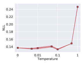
Refer to caption Refer to caption
(a) Test negative log-likelihood (b) Test error
Figure 6: NLL and error (%) as a function of temeprature on CIFAR-10 using cSGLD. The best performance of both NLL and error is achieved at T=0.1𝑇0.1T=0.1.
Refer to caption Refer to caption
(a) Test negative log-likelihood (b) Test error
Figure 7: NLL and error (%) as a function of temeprature on CIFAR-100 using cSGLD. The best performance of both NLL and error is achieved at T=0.01𝑇0.01T=0.01.

Appendix K Experimental Setting Details

K.1 Bayesian Logistic Regression

For both cSGLD and cSGHMC, M=100𝑀100M=100, β=0.01𝛽0.01\beta=0.01. For cSGLD, α0N=1.2,0.5,1.5subscript𝛼0𝑁1.20.51.5\alpha_{0}N=1.2,0.5,1.5 for Austrilian, German and Hear respectively. For cSGHMC α0N=0.5,0.3,1.0subscript𝛼0𝑁0.50.31.0\alpha_{0}N=0.5,0.3,1.0 for Austrilian, German and Hear respectively. For SG-MCMC, the stepsize is a𝑎a for the first 5000 iterations and then switch to the decay schedule (1) with b=0𝑏0b=0, γ=0.55𝛾0.55\gamma=0.55. aN=1.2,0.5,1.5𝑎𝑁1.20.51.5aN=1.2,0.5,1.5 for Austrilian, German and Hear respectively for SGLD and aN=0.5,0.3,1.0𝑎𝑁0.50.31.0aN=0.5,0.3,1.0 for Austrilian, German and Hear respectively for SGHMC. η=0.5𝜂0.5\eta=0.5 in cSGHMC and SGHMC.

Assume that we collect {θb}b=1Bsuperscriptsubscriptsubscript𝜃𝑏𝑏1𝐵\{\theta_{b}\}_{b=1}^{B} samples. Effective sample size (ESS) is computed by

ESS=B1+2sB1(1sB)ρsESS𝐵12superscriptsubscript𝑠𝐵11𝑠𝐵subscript𝜌𝑠\text{ESS}=\frac{B}{1+2\sum_{s}^{B-1}(1-\frac{s}{B})\rho_{s}}

where ρssubscript𝜌𝑠\rho_{s} is estimated by

ρ^s=1σ^2(Bs)b=s+1B(θbμ^)(θbsμ^)subscript^𝜌𝑠1superscript^𝜎2𝐵𝑠superscriptsubscript𝑏𝑠1𝐵subscript𝜃𝑏^𝜇subscript𝜃𝑏𝑠^𝜇\hat{\rho}_{s}=\frac{1}{\hat{\sigma}^{2}(B-s)}\sum_{b=s+1}^{B}(\theta_{b}-\hat{\mu})(\theta_{b-s}-\hat{\mu})

Similar to Hoffman & Gelman (2014), σ^2superscript^𝜎2\hat{\sigma}^{2} and μ^^𝜇\hat{\mu} are obtained by running an independent sampler. We use HMC in this paper.

K.2 Bayesian Neural Networks

For SG-MCMC, the stepsize decays from 0.1 to 0.001 for the first 150 epochs and then switch to the decay schedule (1) with a=0.01,b=0formulae-sequence𝑎0.01𝑏0a=0.01,b=0 and γ=0.5005𝛾0.5005\gamma=0.5005. η=0.9𝜂0.9\eta=0.9 in cSGHMC, Snapshot-SGDM and SGHMC.

K.3 Uncertainty Evaluation

For both cSG-MCMC and Snapshot, M=4𝑀4M=4. β=0.8𝛽0.8\beta=0.8 in cSG-MCMC. α0N=0.01subscript𝛼0𝑁0.01\alpha_{0}N=0.01 and 0.0080.0080.008 for cSGLD and cSGHMC respectively. For SG-MCMC, the stepsize is a𝑎a for the first 50 iterations and then switch to the decay schedule (1) with b=0𝑏0b=0, γ=0.5005𝛾0.5005\gamma=0.5005. aN=0.01𝑎𝑁0.01aN=0.01 for SGLD and aN=0.008𝑎𝑁0.008aN=0.008 for SGHMC. η=0.5𝜂0.5\eta=0.5 in cSGHMC, Snapshot-SGDM and SGHMC.