simsurvey: Estimating Transient Discovery Rates for the Zwicky Transient Facility

Abstract

When planning a survey for astronomical transients, many factors such as cadence, filter choice, sky coverage, and depth of observations need to be balanced in order to optimize the scientific gain of the survey. Here we present a software package called simsurvey for simulating the supernova lightcurves that are expected based on a survey strategy, which can then be used to determine the potential for discoveries of each strategy in question. The code is set up in a modular fashion that allows easy modification of small details of the survey and enables the user to adapt it to any survey design and transient template that they wish to use in planning their survey. As an example of its utility, we use simsurvey to simulate the lightcurve of several types of supernovae that the recently started Zwicky Transient Facility (ZTF) is expected to find and compare the results to the discoveries made during its early operations. We conclude that ZTF will find thousands of bright supernovae per year, of which about 10 could potentially be found with two days of explosion. Over the course of three years the survey will obtain lightcurves of about 1800 type Ia supernovae with $z<0.1$ that can be used as distance indicators in cosmology if they are spectroscopically classified using additional telescopes. In a comparison to detections from the ZTF public survey, we found good agreement with the numbers of detections expected from the simulations.

1 Introduction

Over the past decades the search for transient astronomical events, such as supernovae, has evolved from the occasional serendipitous discovery to systematic searches using dedicated telescopes designed to find transients. Such surveys, including the Supernova Legacy Survey (SNLS; [1]), the Sloan Digital Sky Survey II (SDSS-II, [2]), Palomar QUEST [3], Skymapper [4], PanSTARRS [5], the All-Sky Automated Survey for Supernovae (ASAS-SN; [6]), the Asteroid Terrestrial-impact Last Alert System (ATLAS; [7]), the Dark Energy Survey (DES; [8]), and the (intermediate) Palomar Transient Factory (PTF/iPTF; [9]), have systematically discovered thousands of supernovae.

One of the latest transient surveys is the Zwicky Transient Facility (ZTF, [10, 11]) using the Palomar 48-inch Schmidt telescope. The same telescope has previously been used for PTF/iPTF and has now been equipped with a new camera that allows full usage of its 47 sq. deg. field of view and shorter exposures. With this improvement in survey speed, ZTF can practically cover the whole observable sky in a single night (or observe the same location repeatedly), reaching $\sim$ 20.5 mag in 30 second exposures. This makes it an excellent survey for a great range of transient studies because it can survey a large nearby volume, in which spectroscopy is easier to obtain, by covering the sky rapidly. ZTF can find supernovae within hours of explosion, with the potential for discovering new types of events that evolve much faster and it can also collect a large and well-controlled sample of supernovae for studies of their rates and population properties. ZTF can also, in case of type Ia supernovae, provide accurate measurements of distances in the local universe that can be used for cosmological inference.

In order to make the best use of an instrument like the ZTF camera, careful planning of the survey strategy is required, especially when varied scientific interests need to be balanced. For previous surveys the strategy has been optimized using Monte Carlo methods that generate lightcurves of transient that will be obtained by the survey based on the survey strategy, e.g. using the package SNANA [12] for DES [13, 14] and the Wide-Field InfraRed Survey Telescope (WFIRST, [15]). Additionally this technique can be used to determine the survey efficiencies and biases as has been done for DES [16] and the joint analysis of SDSS and SNLS SNe Ia data [17].

In this paper we present a Python package, simsurvey, that can be used for this type of analysis. Based on these lightcurves we can then define metrics for how well the survey works for a given science case, e.g. how many SNe can be found shortly after explosion or for how many SNe Ia will we obtain the lightcurve coverage required for cosmology. We will use ZTF as an example of a survey, for which we used the package to optimize the strategy. However, we would like to point out that this package can be used for any survey and is not restricted to ZTF. All parameters that differ between surveys, e.g. CCD layout or field grid definition, can be adjusted easily.

In section 2 we present the simsurvey Python package that is used to simulate the lightcurves that we expect from ZTF. We outline the simulation in 3 and show the results in section 4. The scientific implications of the simulations are discussed in section 5 and compared to the first discoveries by ZTF in section 6. Finally we summarize our findings in section 7.

2 Survey simulation software simsurvey

The lightcurves are simulated using Python code mostly from the packages sncosmo [18] and astropy [19, 20]. This code has been released on PyPI as simsurvey [21] and will be described below. When simulating the lightcurves of a whole survey, the following input will be required:

• A survey schedule containing the time, pointing and filter of each exposure. Additionally sky brightness and zero points can be provided for each observation in the schedule, e.g. based on a weather model, or otherwise these parameters can be set to a default value.

• A transient model, i.e. a time-series of spectral energy distributions (SEDs) from which the photometry of the transients can be calculated. The SEDs of the transient need to be provided over a sufficient wavelength range such that all filters used in the survey schedule fall into it for the whole redshift range of the simulation.

• A function that allows us to sample the transient model parameters, e.g. peak magnitude, lightcurve width or host galaxy extinction for each transient, from a distribution modeling the transient population.

As a first step, transients are placed at redshifts sampled from a distribution based on the volumetric rate as a function of redshift up to a redshift cutoff. The total number of transients is based on the integrated rate as well as the time span of the survey and the solid angle it covers but it can also be fixed to any arbitrary value instead of using the absolute rate to determine it. In this case the relative redshift distribution will remain the same. For each transient the code draws the coordinates on the sky from a uniform distribution on the unit sphere that can be limited in right ascension and declination, and should be chosen to cover the whole survey footprint. The Milky Way can be excluded using a simple cut in Galactic latitude $b$, but this is not necessary in order to exclude transients behind the Galactic plane because the code will determine the extinction by Galactic dust for all transients based on the maps from [22] and apply extinction to the transient model. Thus while lightcurves for transients behind the Milky Way would be simulated if the survey schedule points in that direction, they will generally be below the detection threshold due to extinction. Lastly a random Julian date for the $t_{0}$ parameter (time of peak or time of explosion) of the model is drawn from a uniform distribution based on the time span of the survey.

Based on the redshifts and the transient template the other parameters for the lightcurve simulation are then determined. For several built-in templates of sncosmo, simple distributions of the model parameter reflecting the transient population have been built into simsurvey but both the template and the distribution can easily be replaced by the user. Instead of using one of the built-in templates, a custom transient template can be defined using sncosmo. These templates can, for instance, be based on SEDs obtained from simulations of the merger of two neutron stars. Alternatively analytic functions can also be used to define the model. An example of this is using Planck’s law of black-body radiation along with formulae for the evolution of temperature and radius of the photosphere of a transient. Therefore, simsurvey can be used to simulate both well-studied SNe and hypothetical transients that are significantly rarer.

Distributions for all transient model parameters except the redshift and $t_{0}$ can be defined by a single Python function. The list of model parameters usually includes the flux normalization of the model – based on the transient’s absolute magnitude distribution and its distance modulus – and model-specific parameters, e.g. the SALT2 [23] stretch and color parameters $x_{1}$ and $c$. Additionally, sncosmo models can be extended by propagation effects such as extinction by dust in the host galaxy (modeled by a wavelength-dependent extinction law). These effects add further parameters to the model, e.g. $E(B-V)$ and $R_{V}$.

Using this set of transient model parameters the code can then simulate lightcurves based on the survey schedule. First a list of survey fields, in which a transient is located, is generated for each transient. For this, the shape of the survey’s field of view must be provided. In the simplest case this can be the projection of rectangular field of view onto the sky (defined by its width and height in degrees) but additionally the code can match the transients to individual CCD chips of a camera if its layout is provided. simsurvey can therefore also be used for surveys with a field of view that is more complicated than a simple rectangle, e.g. LSST, and also account for losses due to the gaps between the CCD chips. Once the fields in which each transient is located have been determined, a list of observations that include its coordinates is generated. If the survey strategy does not use a fixed grid of fields for observations, the pointings can also be given by just their coordinates, which will then be matched with the transients individually.

The observations list is further restricted by the minimum and maximum times relative to $t_{0}$ for which the template is defined (multiplied by $(1+z)$ to account for time dilation) in order to limit the lightcurve to the relevant parts if the survey covers a much longer time scale. The time frame is extended by two weeks prior to the definition range of the model, for which the flux is set to a random value based on the sky brightness. This allows us to assess whether we would have pre-explosion limits for the transient in question. This procedure does not account for SN precursor events that may occur for some SN types, especially type IIn, more than two weeks prior to explosion [24]. However, such a precursor could be added to an existing SN model using sncosmo. For all other pointings to the transient, the flux is calculated based on the template and the passbands used by the survey and then perturbed by noise terms based on the sky brightness, the Poisson noise expected for the flux of the transient, and the gain of the instrument.

The lightcurves are then filtered using selection criteria that correspond to the discovery process of transient surveys. The default transient filter requires two $5\sigma$-detections in the same night for a transient to be included in the final output. The requirement of two detections simulates the common asteroid rejection method since the pointings are generally scheduled at least half an hour apart and most asteroids will move sufficiently in that time and thus not be detected as transients at the same coordinates. Lastly useful statistics of the lightcurves will be calculated at the same time, e.g. the time of discovery and the the interval between discovery and the last non-detection, i.e. an observation of the transients locations without a detection.

3 Simulation of the ZTF survey

3.1 Survey schedule

The observing time for the Palomar 48-inch telescope (P48) within ZTF has been allocated to different programs, 40% of the time each go to the public survey and the ZTF partner institutes while the remaining 20% can be used by Caltech staff. In this paper we will disregard the Caltech time and only focus on the extra-galactic parts of the other two programs. A full discussion of the ZTF survey strategy can be found in [25].

The public survey observes the whole visible sky in $g$- and $r$-band at a three-day cadence. Observations of the same field in both bands are scheduled for the same night with sufficient time in between them to distinguish extra-galactic transients from asteroids.

The ZTF partnership time is being used for various smaller extra-galactic surveys. Most of the time is used for a high-cadence survey of $\sim 1600$ sq. deg. with up to six $g$-band observations per night that are separated by at least 30 minutes. This leads to a large number of early transient detections, for some of which we will be able to constrain the time of explosion very well. Furthermore a survey of $\sim 6700$ sq. deg. with a four-day cadence in the $i$-band will be carried out, adding a third filter to many lightcurves from the public survey, which will greatly improve cosmological distance estimates from SNe Ia. Lastly, time is also used for target-of-opportunity (ToO) observations for multi-messenger astronomy, following up on gravitational wave, neutrino or gamma-ray burst triggers.

Simulating full survey operations (including e.g. slew times and filter changes) would be beyond the scope of this study. Instead we select fields (from a grid of 879 fields covering the whole sky) that are observable during a given night and schedule them in a way that corresponds to the cadence of the subprogram without accounting for when exactly the field is at a low airmass during the night. Additionally we did not account for changes in the observing conditions, e.g. due to differences in airmass and sky brightness, but instead set the $5\sigma$-depth of all observations to 20.5 mag. For the simulation we have chosen a period of one year from February 1st, 2018 to January 31st, 2019. The relevant programs of the survey were simulated using the following scheduling:

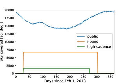
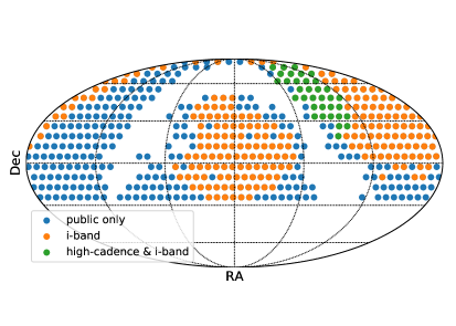
• public: For every third night of the survey we selected all fields that are at an airmass < 2 for at least an hour during that night and that have low Milky Way extinction ($E(B-V)\leq 0.2$). A third of those fields are then scheduled for $g$- and $r$-band observation in the selected night and the remaining fields are observed in the two nights after it.

• high-cadence: This program was limited to 34 of the public survey fields (corresponding to $\sim 1600$ sq. deg.) described above that are observable in at least 95% of the nights throughout an eight-month period from March to October. In addition, the fields were selected such that they are no closer than $50^{\circ}$ to the full moon. (This requirement is lowered based on the phase of the moon.)

• $i$-band: The area covered by the $i$-band program is too large for a single set of fields as used for the high-cadence program. Instead fields were selected such that they can be observed for at least 3.5 months in the period between March and November. For each month we selected 143 fields($\sim 6700$ sq. deg.) to be observed while making sure that individual fields are observed for at least 3 months. A subset of the fields are observable for longer than that, including the 34 fields for the high-cadence program. In total this survey covers $\sim 12000$ sq. deg..

The field selection for each survey and the area covered by it are summarized in Fig. 1. Note that these survey schedules are not using exactly the same field selection as the actual survey (see [25]), e.g. the public extra-galactic survey did not have a cutoff in Milky way extinction but rather in Galactic latitude $b$, and the high-cadence survey ran beyond the end of October where most fields were setting at that time and became more difficult to observe multiple times per night. The simplified surveys used here are, however, still sufficiently close to the actual survey to yield useful estimates.

Figure 1: Left: Solid angle in square degrees monitored by the programs of the survey throughout the year. (The whole sky has a solid angle of $\sim 41000$ sq. deg.) Right: Skymap of the pointings of each program. Note that the marker shape is not the shape of the ZTF field of view and that the true shapes of the ZTF field of view overlap by 13% on average. All shown pointings are in the public survey and all fields in the high-cadence survey are covered by the $i$-band survey as well.

3.2 Lightcurve generation

Table 1: Supernova models used for the simulation and their main simulation parameters. ^†In addition to the intrinsic scatter of SN Ia peak magnitudes, the Tripp relations [26] were used to simulate a realistic population. ^‡To avoid simulating a large number of unrealistically bright SNe IIn, the Gaussian distribution of peak magnitudes was truncated at $1\sigma$ on the brighter-than-average side.

SN type	sncosmo template	Rate [Mpc-3 yr-1]	$M_{B}$ (peak)	$\sigma_{M}$
Ia	salt2	$3\times 10^{-5}$	$-19.3$	$0.1^{\dagger}$
Ib/c	nugent-sn1bc	$2.25\times 10^{-5}$	$-17.5$	$1.2$
IIn	nugent-sn2n	$7.5\times 10^{-6}$	$-18.5$	$1.4^{\ddagger}$
IIP	nugent-sn2p	$1.2\times 10^{-4}$	$-16.75$	$1$

For the lightcurve simulations we focused on type Ia supernovae and common types of core-collapse SNe, specifically types Ib/c, IIn and IIP. The templates were chosen from the sets of built-in model of sncosmo and are summarized in Table 1. The SN models were scaled to peak $B$-band magnitudes based roughly on the distribution reported in [27]. In addition extinction by dust in the host galaxy was added to the models for core-collapse supernovae. For this we used the extinction law of Cardelli, Clayton & Mathis [28] with a relatively steep slope $(R_{V}=2)$ and $E(B-V)$ drawn from an exponential distribution with a rate $\lambda=0.11$ (as reported by [29]). Since the model used for SNe Ia (SALT2, [23, 30]) uses an effective color term that includes host galaxy extinction, we did not include this effect again. Instead values for the model parameters $x_{1}$ (“stretch”) and $c$ (“color”) were drawn from Gaussian distributions centered around 0 with a width $\sigma$ of 1 and 0.1, respectively. Based on these values the peak magnitude of the SN Ia is adjusted according to the Tripp relations [26] that correlate the peak brightness with lightcurve slope and color and need to be corrected when using SNe Ia as distance indicator. The coefficients were chosen to be close to the usual results of cosmological analyses, e.g. [30], $\alpha=0.13$ for the stretch and $\beta=3$ for the color.

The transients were distributed in redshift assuming a constant volumetric rate. This assumption is valid because the SNe detected by ZTF will mostly be near-by. At the farthest, some SNe Ia may be found out to $z=0.2$ but the bulk is around $z=0.1$. The coordinates for the transients are drawn from a uniform distribution (by solid angle) down to declinations $\delta=-30^{\circ}$, which is the farthest south that the schedule covers. The Galactic Plane is not explicitly excluded in the transient placement but an extinction term based on dust in the Milky Way is added to the model and therefore transients behind the Galactic Plane (as described in section 2) are less likely to be observed. The total number of simulated transients was calculated based on the redshift-integrated volumetric rate multiplied by the fraction of the sky on which the transients are simulated (75% in this case) and the time range for the $t_{0}$ parameter of the model, i.e. either time of explosion or of peak brightness, which is chosen to begin one month before the schedule and end one month after it in order to account for cases, for which only the rising or declining part of the lightcurve is observed. The rates are listed in Table 1. For SNe Ia we used the value from [31] and for the core-collapse SN rate the one from [32]. We note that the value for the latter ($1.5\times 10^{-4}~{}\mathrm{Mpc}^{-3}\mathrm{yr}^{-1}$) is larger than the values reported in [31] but still with the typical uncertainties for these measurement. The core-collapse SN rate was split the following way: 80% type IIP (also including the type IIL rate), 15% type Ib/c, and 5% type IIn. This roughly corresponds to the relative rates of these subtypes according to [33].

The simulation was run 100 times for each transient type and a one-year survey plan in order to build up larger statistics. We did not use any model to predict the sky brightness but just fixed its contribution to the flux uncertainty at a value corresponding to a $5\sigma$-depth of 20.5 mag instead. At first we assumed perfect observing conditions for every night when generating the lightcurves but then certain epochs are removed from them based on the iPTF pointing history for 2016, therefore also accounting for losses of observation time that are not due to weather. For simplicity, we only removed full nights and did not attempt to create a schedule that accommodate for weather losses in any way, e.g. by rescheduling observations that were missed. All results have been normalized to the expectation for one year of ZTF operations as described in section 3.1. The script required to rerun the simulations can be found at https://github.com/ufeindt/simsurvey-paper-scripts.

4 Results

4.1 Detection of young transients

Figure 2: Left: Discovery phases $p_{\rm det}$ w.r.t. $B$-band peak for the simulated SNe Ia. The thick line shows the SNe in the public and $i$-band (“low-cadence”) surveys while thin line shows only the ones found in high-cadence fields. Right: Time of discovery $t_{\rm det}$ w.r.t. explosion for CC SNe. Thick lines again show SNe in low-cadence surveys while thin lines show high-cadence fields.

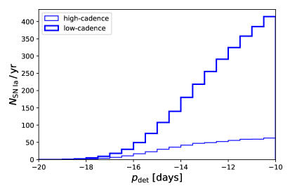
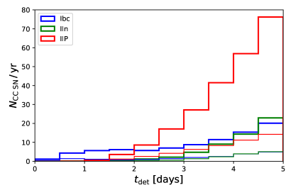
Given the large survey speed of ZTF, many transients will be discovered very shortly after explosion, some potentially in the same night. Many early discoveries are expected to be made using the public survey alone but the high-cadence part of the partnership survey will allow even earlier detections and give tighter constraints on the time of explosion because the coordinates of the transient will have been observed during the previous night (instead of three nights ago) or potentially even earlier the same night.

Table 2: Expected numbers per year of SNe discovered early for varying detection phases $p_{\rm det}$ w.r.t. $B$-band peak for SNe Ia or times of detecion $t_{\rm det}$ w.r.t. explosion for CC SNe found either in the high-cadence survey or in the low-cadence parts of the extra-galactic survey, i.e the public and $i$-band surveys. (The different notations are due to the differences in definition of $t_{0}$, i.e. the time of peak or the time of explosion, respectively.)

SNe Ia	$p_{\rm det}<-15$	$p_{\rm det}<-17$	$p_{\rm det}<-18$	$p_{\rm det}<-19$
high-cadence	65	7.84	1.78	0.11
low-cadence	191.36	18.1	3.2	0.19
	$t_{\rm det}<5$	$t_{\rm det}<3$	$t_{\rm det}<2$	$t_{\rm det}<1$
SNe Ib/c
high-cadence	19.28	5.96	3.62	1.85
low-cadence	66.42	24.02	13.69	3.65
SNe IIn
high-cadence	14.04	1.29	0.34	0.06
low-cadence	41.49	3.17	0.79	0.1
SNe IIP
high-cadence	48.21	8.22	1.43	0.02
low-cadence	183.53	21.8	2.91	0.02

To determine the phase at which phase a simulated supernova was detected, we recorded the time of the second $5\sigma$-detection of the SN and subtracted the parameter $t_{0}$ for the transient model used. For SALT2 this is the time of $B$-band maximum but the Nugent models of the CC SNe this is the time of explosion. Thus, we show the distributions for SNe Ia and CC SNe in separate panels of Fig. 2. The histograms were limited to five days after explosion for the CC SNe and to phases $p<-10$ days for SNe Ia. The plots show discoveries from the high-cadence survey compared to the rest of the survey. Since the high-cadence survey covers an area about an order of magnitude smaller than the public survey, we expect to find fewer transient in total in this limited area. However, we expect the discoveries to be earlier, on average, for a higher cadence. Accordingly we find that the median phase of SN Ia discovery relative the $B$-band maximum is -8.4 days in the high-cadence survey opposed to -5.6 days for the whole survey (including partnership time). The expected numbers of early discoveries per year is shown in Table 2. We expect to find about five SNe Ia at phases earlier -18 days and about 250 at -15 days. Of the CC SNe only SNe Ib/c appear likely to be found within a day (about five or six per year). A similar number of SNe IIP may be discovered within two days but only one SN IIn is expected.

While the statistics discussed so far show that ZTF will produce lightcurves of transients starting very close to explosion, we have not yet addressed the issue how determine that these transients are potentially young. The most important metric for that is the time since the last pointing to the transient’s coordinates, for which it was not detected. This information was extracted for the simulated lightcurves along with the phases of detection as the interval between the first of the required two detections at $5\sigma$-level and the previous lightcurve point that was below the threshold and therefore would in reality only be an upper limit. In a more realistic setting, we would also need to account for the varying depth of the observation and only count limits that are enough to exclude something as bright as the newly discovered transient. Since we assumed a constant depth for simplicity, we do not require that level of precision in our approach.

However, the time since the last non-detection in and of itself is insufficient to find early transients. Many SNe that are too distant to be detected early will also cross the detection threshold between two nights or during the same night. The simulations show for example that 800 SNe Ib/c will be found with a non-detection in the previous night or later while only 5.5 are expected to be found in the within a day of explosion. To weed out distant SNe, a redshift cut needs to be applied as well. For this we will assume that the host galaxy redshift can always be obtained from catalogs. Additionally the use of catalogs will allow us to filter out known active galactic nuclei, which are another possible source of contamination of the transient sample. In reality this will not be possible in all cases because the host galaxy cannot always be identified and redshift catalogs are not complete. Therefore only a certain fraction of the simulated SNe can be discovered this way. To estimate this fraction, we can use the findings of ZTF’s predecessor surveys, PTF and iPTF. Of the SNe (CC and Ia) found by them 25% could be associated with a galaxy that has a spectroscopic redshift in the SDSS catalogs and 78% have a host galaxy with a photometric redshift [34]. Therefore, this efficacy of these criteria will mostly rely on photometric redshifts.

Table 3: Expected number per year of SNe observed early ($p_{\rm det}<-17$ days for SNe Ia and $t_{\rm det}<2$ days for CC SNe) and/or with a non-detection the night before or during the same night ($\Delta t_{\rm non-det}<1.5$ days).

	$z<0.03$			$z<0.05$
	early &	only	only	early &	only	only
	non-det.	early	non-det.	non-det.	early	non-det.
SNe Ia
high-cadence	2.13	2.53	4.03	4.9	5.52	19.81
low-cadence	1.65	9.79	7.33	3.16	15.98	35.65
SNe Ib/c
high-cadence	1.42	1.73	3.56	2.28	2.78	16.04
low-cadence	1.30	7.18	6.81	2.06	11.0	31.25
SNe IIn
high-cadence	0.24	0.28	0.94	0.3	0.34	4.71
low-cadence	0.15	0.77	1.64	0.15	0.79	8.02
SNe IIP
high-cadence	1.21	1.29	17.32	1.32	1.42	73.35
low-cadence	0.54	2.79	32.44	0.56	2.91	132.24

Using these criteria for selection the advantages of the high-cadence survey for finding early transients become much more obvious. For instance, about 89% of the SNe Ia at redshift $z<0.05$ that are found at a phase $p<-17$ days in the high-cadence survey also have an observation without a detection during the same night or the night before (see Table 3). While basing the selection only on low redshift and the time since last non-detection fails to filter out all SNe that are found later than the selected phase, this number is only about three times larger (14.91 later-than-specified discoveries per year compared to 4.9 per year discovery before the selected phase cut). For the rest of the extra-galactic survey (public and $i$-band surveys), on the other hand, only about 20% of the early SNe can be found this way.

4.2 Spectroscopically complete survey of bright transients

For studies of the populations of transients in the local universe it is essential to build catalogs of spectroscopically confirmed SNe to fixed magnitude limit. This will help us to account for biases in the higher-redshift parts of our data (e.g. for cosmological constraints) and the redshift completeness of local galaxy catalogs (see [35]).

In addition to the wide-field camera on P48, the ZTF collaboration has access to time with the Spectral Energy Distribution Machine (SEDM; [36]), an integral field spectrograph mounted on the Palomar 60-inch (P60) telescope. This will allow the spectroscopic classification of all transients found by ZTF to a peak brightness of 18.5 mag and potentially fainter. Based on our simulations (see Table 4), we expect 1768 SNe brighter than 18.5 mag (with $\sim$ 50% of those brighter than 18 mag) and about as many (1702) between that and 19 mag. We find that such a survey will probe the population of SNe out to a redshift of 0.1 (in case of SNe Ia, see left panel of Figure 3) with median redshifts around 0.05, see Table 4.

Table 4: Expected number per year of SNe peaking brighter than a given magnitude in both $g$- and $r$-band and their median redshifts $z_{\rm med}$. Note that these numbers are based on the brightest magnitudes in the simulated lightcurve (typically within one or two day of peak brightness) and not on the peak brightness of the model used for the simulation.

	$\textrm{mag}<18$		$\textrm{mag}<18.5$		$\textrm{mag}<19$		$\textrm{mag}<19.5$		$\textrm{mag}<20$
	$N$	$z_{\rm med}$	$N$	$z_{\rm med}$	$N$	$z_{\rm med}$	$N$	$z_{\rm med}$	$N$	$z_{\rm med}$
Ia	568	0.045	1116	0.056	2218	0.071	4352	0.090	8500	0.114
Ibc	115	0.040	216	0.049	405	0.061	747	0.074	1373	0.088
IIn	52	0.038	103	0.048	205	0.061	409	0.077	840	0.099
IIP	173	0.023	333	0.029	642	0.036	1222	0.045	2339	0.055

Figure 3: Left: Redshift distribution of SNe Ia for various peak magnitude cuts. Right: Redshift distribution of SNe Ia that pass the cosmology criteria.

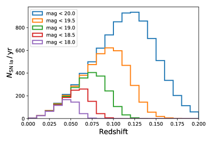
4.3 SN Ia lightcurves for cosmology

For cosmology, we are interested in obtaining SNe Ia lightcurves that provide precise measurements of the distance modulus. As SNe Ia are not perfect standard candles but require an amount of standardization based on their width and color [37], we can only use lightcurves that are well sampled around peak in all three bands. Thus, all SNe in this sample are in the fields of the $i$-band program. Additionally we restrict this dataset to SNe at redshift $z<0.1$ because we will not have a flux-complete sample beyond that redshift and therefore a cosmological analysis would be affected by Malmquist bias. The full set of criteria is as follows:

• The redshift is less than 0.1.

• The first detection is at least 10 days prior to $t_{0}t$, i.e. the time $B$-band maximum.

• The last observed epoch is at 30 days after maximum.

• There are at least three $i$-band pointings between 10 days prior to and 15 days after maximum.

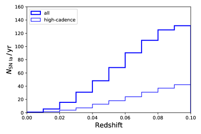
Based on 100 simulations using the SALT2 model, we find a median number of 626 SNe Ia matching these criteria. Their redshift and peak magnitude distribution are shown in the right panel of Figure 3. The median redshift is 0.075 and the median peak brightness is 18.5 mag in $g$-band. Thus only half of these SNe will be covered when obtaining a spectroscopically complete samples described in section 4.2. The remaining SNe Ia will thus have to be classified using other resources. As ZTF will run for three years, we can expect to collect $\sim 1800$ lightcurves of the quality described above. The cosmological implications of such a dataset will be discussed in the next section.

5 Discussion

In the previous section we have shown how ZTF will provide both many early discoveries of transients and large datasets of the most common type of SNe. The former will greatly help us understand the physics of relativistic explosions and supernovae but a full discussion of this would be beyond the scope of this paper. The latter, on the other hand, can be summarized by some cases in which the sample of SN Ia lightcurves described in section 4.3 will benefit cosmological studies.

5.1 Dark energy constraints

Figure 4: Left: Expected confidence regions ($68.3\%$ CL) of the dark energy e.o.s. parameters $w_{0}$ and $w_{a}$ for a flat $w_{0}w_{a}$CDM cosmology model for WFIRST with and without the addition of a ZTF low-redshift SN Ia data set. The solid red line assumes that the datasets are both perfectly calibrated while the other red lines show the effect of a systematic uncertainty $\sigma_{\rm sys}$ of 0.005 mag (dashed line) or 0.01 mag (dotted line). Right: Expected uncertainties for a peculiar velocity dipole derived from three years of ZTF SN Ia data as a function of the maximum redshift used in the fit. The error bars correspond to the nMAD of all possible combinations of three out of the 100 simulations that were run. The solid line shows the expected size of a dipole from $\Lambda$CDM structure formation, showing the uncertainty required to determine whether the measured dipole matches the expectation for an isotropic universe.

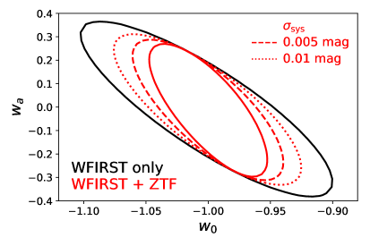
A large, low-redshift data set of SNe Ia will greatly improve the constraints on the dark energy equation of state (e.o.s.) by anchoring the Hubble diagram. This can best be demonstrated by comparing how the constraints from a future survey of higher-redshift SNe Ia, e.g. by the Wide-Field InfraRed Survey Telescope (WFIRST), improve when a low-redshift sample is added to the data set. We used the distance modulus uncertainties and systematic covariances, binned in redshift, from the simulations presented in [15]. We removed the bins at redshifts $z<0.1$ because these bins are based on simulations of the Foundation survey [38] and here we wish to investigate the impact that ZTF can have on its own. For ZTF we use the equations in Appendix C.1 of the final report by the Science Definition Team and WFIRST Project [39] to determine the binned uncertainties we expect from ZTF,

$$\sigma_{\rm stat}=\sqrt{\frac{(\sigma_{\rm meas})^{2}+(\sigma_{\rm int})^{2}+(\sigma_{\rm lens})^{2}}{N_{\rm SN}}},$$ (5.1)

where $\sigma_{\rm meas}=0.08$ mag, $\sigma_{\rm int}=0.08$ mag, $\sigma_{\rm lens}=0.07\cdot z$ mag, and the values for $N_{\rm SN}$ are binned numbers of SNe Ia shown in the right panel of Figure 3, multiplied by a factor three for the expected duration of the survey.

As a metric of the quality of the dark energy constraints, we calculate the confidence regions for the parameters $w_{0}$ and $w_{a}$ of a flat $w_{0}w_{a}$CDM cosmology model [40, 41], i.e. a model where the dark energy e.o.s. evolves with redshift and is parameterized as

$$w=w_{0}+w_{a}\frac{z}{1+z}.$$ (5.2)

This method is similar to the method defined by the Dark Energy Task Force [42], using the inverse area of the confidence region as a figure of merit (FoM). As a fiducial model we assume $w_{0}=-1$ and $w_{a}=0$, which corresponds to a flat $\Lambda$CDM cosmology. To constrain the estimate further we include a simple Gaussian prior on the matter density parameter $\Omega_{\rm M}$ based on the most recent results from the Planck Collaboration [43], setting its width to 0.007. As the binned uncertainties from our ZTF simulations do not include an estimate of the systematic uncertainties of the distance estimates (e.g. from calibration uncertainties or evolution of SN Ia brightness with redshift), we included a offset term that shifts the ZTF data relative to WFIRST as a nuisance parameter in the likelihood. For the prior on this offset we assumed two cases, both Gaussian, one with a width of 0.005 mag and the other with 0.01 mag. The latter value is our target for the calibration precision, which is the main contributor to the systematic uncertainties in SN Ia cosmology, while the other is a more optimistic scenario.

The resulting contours are shown in Figure 4. Including ZTF data in such an analysis will greatly improve the constraints, increasing the figure of merit by 30% compared to WFIRST alone, given a systematic uncertainty for ZTF of 0.01 mag (73% for 0.005 mag).

5.2 Local anisotropy

An addition to constraining dark energy, the data set that ZTF will collect will allow more precise measurement of structure and anisotropy in the local universe. One possible test of anisotropy is by looking for a peculiar velocity dipole or bulk flow in the low-redshift data. If this dipole exceeds the expectation from $\Lambda$CDM structure formation this could be indicative of effects beyond the standard model of cosmology.

To estimate the uncertainties of a dipole estimate using ZTF data, we apply the same method as in [44], where the dipole formula from [45] was used to determine the effect of peculiar velocities on the luminosity distance:

$$\tilde{d}_{L}(z,\vec{n},\vec{v}_{d})=d_{L}(z)+\frac{(1+z)^{2}}{H(z)}\vec{n}\cdot\vec{v}_{d},$$ (5.3)

where $d_{L}(z)$ is the unperturbed luminosity distance, $\vec{n}$ is the radial unit vector corresponding to the SN’s coordinates and $\vec{v}_{d}$ is the bulk flow velocity vector. The velocity vector could then be determined by statistically inference such as minimizing the following $\chi^{2}$ expression:

$$\chi^{2}=\sum\limits_{i}\frac{\left|\mu_{i}-5\log_{10}\left(\left(d_{L}(z_{i})+\frac{(1+z_{i})^{2}}{H(z_{i})}\vec{n}\cdot\vec{v}_{d}\right)/\left(10\mathrm{pc}\right)\right)\right|^{2}}{\sigma_{i}^{2}},$$ (5.4)

where $\mu_{i}$ is the measured distance modulus of a SN Ia and $\sigma_{i}$ is its uncertainty, for which we use the same formula as in the previous section (equation 5.1). For this expression the resulting covariance matrix of the velocity dipole is then expressed as

$$\mathrm{Cov}(\vec{v}_{d})=\left(\sum\limits_{i}\left(\frac{5(1+z_{i})^{2}}{\ln 10\tilde{d}_{L}(z_{i})H(z_{i})\sigma_{i}}\right)^{2}\vec{n}_{i}\vec{n}_{i}^{T}\right)^{-1}.$$ (5.5)

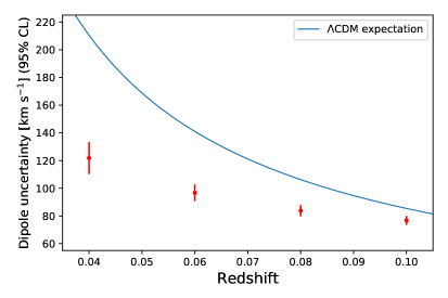
In order to sample how the differences in redshift distribution and sky coverage between the 100 one-year simulation affect the dipole as it would be determined by a three-year survey, we calculated this covariance matrix for all 161700 possible combinations of three out of the 100 simulations, using several redshift cutoffs for the data to see the evolution of the uncertainty with the radius of the sphere, in which the bulk flow is determined. Since the expression in equation (5.4) is not completely linear in velocity, the uncertainty depends on the best-fit value. Thus we chose to assume a velocity dipole in the direction of the Shapley supercluster, which roughly corresponds to the direction most studies of the bulk flow find. For the amplitude we assumed that the velocity decreases with the radius of the sphere as $v\sim 250\left(\frac{100\mathrm{Mpc}}{d}\right)\mathrm{km~{}s^{-1}}$, where $d$ is the comoving distance from the observer. This is the approximate expectation for a dipole arising from random fluctuations in $\Lambda$CDM (see e.g. [46]). The right panel of Fig. 4 shows the uncertainty of the bulk flow for the selection redshift cutoffs as well as the expected value from structure formation. This shows that the ZTF SN Ia data set will allow us to constrain the bulk flow at the level of what we expect to find due to structure formation.

6 Comparison to first ZTF detections

Figure 5: Histograms of the SALT2 “stretch” parameter $x_{1}$ (left panel) and color parameter $c$ (right panel) based on lightcurve fits to ZTF public alert data for selected fields and detection in July 2018 (blue solid bars) and simulated lightcurves based on SN models restricted to the same fields and time of detection.

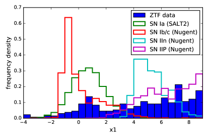
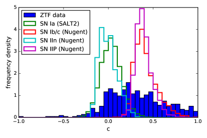
Since ZTF started observing in early 2018, many transients have already been found and these discoveries can thus be compared to the predictions from the simulations in this paper. However, at this time a full measurement of supernova rates would be beyond the scope of this paper. We will therefore limit this section to a quick comparison of how many SNe were found in a specific set of fields in July. These fields were chosen because that had fully-built reference images by the beginning of July and were observed until the end of the month. The ZTF discoveries were extracted from the public alert stream using the AMPEL broker [47]. Since we used no ZTF partnership data in this analysis, we also removed the partnership epochs from simulated lightcurves to match the cadence. For both the alerts and the simulated lightcurves we required that there were at least five points brighter than 20 mag during the month of July.

For each selected lightcurve, we extracted basic parameters by fitting the SALT2 model to it. We further included the redshift as a fit parameter because a host redshift cannot be obtained automatically without a greater effort that would be beyond the scope of this section. While this model is intended for standardizing SNe Ia brightnesses for cosmological distance measurements, its fit results can also be used to distinguish SN types. The “stretch” parameter $x_{1}$ and the color parameter $c$ are most useful for this because different types of SNe have different rise times and color indices and thus SNe of types other than Ia will not have a distribution centered on 0 in one of these parameters or both. The absolute peak magnitude of a transient could also be used to distinguish SN types but the photometric redshifts obtained from the fit are too inaccurate to give a useful distribution. Based on the distributions of the lightcurve parameters for the simulated SNe (see Figure 5, we find that transients with $-2<x_{1}<2$ and $-0.2<c<0.2$ are most likely to be SNe Ia. While a selection based on these criteria is not expected to yield a complete or pure sample, it is a sufficient for a simple comparison. Based on these criteria we find 37 transients among the filtered ZTF alerts, which is in good agreement with the 44 SNe (almost exclusively of type Ia) expected based on the simulated data sets. We have further checked whether these object were in fact SNe Ia, finding that 19 of them have been spectroscopically typed as SNe Ia while no spectra were taken of the rest.

7 Conclusion

We have presented a software package, simsurvey, for the simulation of lightcurves for photometric transient surveys. The package can be used for most types of extra-galactic transients as long as the user provides a spectral time series, from which the photometry can be synthesized at various redshifts. Additionally the package contains built-in simulators for common supernova types such as SNe Ia. Furthermore the code is not specific to any particular survey and can be used to simulate lightcurves based on any schedule and telescope configuration.

As an example of its utility, we have simulated the lightcurves of type Ia supernovae and several types of core-collapse supernovae as they are expected to be observed by the Zwicky Transient Facility. The simulations included both the wide public survey as well as partnership surveys focusing on smaller areas but using a higher cadence or an additional filter. Our significant findings include:

• ZTF will find thousands of SNe per year, about 1800 of which will peak at a magnitude < 18.5 mag.

• ZTF will be able to find on the order of 10 very young SNe per year and will be able to identify them as young through a combination of host redshifts (from catalogs) and the time since the last observation of its coordinates without a detection (mostly driving by high-cadence observations of a limited set of fields).

• Within a year about 600 SNe Ia with sufficient lightcurve quality for cosmology will be found. A data set built up over the course of three years will contain about an order of magnitude more low-redshift supernovae than current samples and will be essential for future studies of the dark energy equation of state as well as studies of the local anisotropy.

Lastly, we have compared our simulations to part of the discoveries made so far by ZTF based on the public alert stream for a month and a limited number of fields that had reference images by the start of July. Based on this comparison we found a good agreement between our simulations and the first discoveries of the survey.

References

- [1] P. Astier, J. Guy, N. Regnault, R. Pain, E. Aubourg, D. Balam et al., The Supernova Legacy Survey: measurement of M, Λ and w from the first year data set, A&A 447 (2006) 31 [astro-ph/0510447].
- [2] J. A. Frieman, B. Bassett, A. Becker, C. Choi, D. Cinabro, F. DeJongh et al., The Sloan Digital Sky Survey-II Supernova Survey: Technical Summary, AJ 135 (2008) 338 [0708.2749].
- [3] S. G. Djorgovski, C. Baltay, A. A. Mahabal, A. J. Drake, R. Williams, D. Rabinowitz et al., The Palomar-Quest digital synoptic sky survey, Astronomische Nachrichten 329 (2008) 263 [0801.3005].
- [4] S. C. Keller, B. P. Schmidt, M. S. Bessell, P. G. Conroy, P. Francis, A. Granlund et al., The SkyMapper Telescope and The Southern Sky Survey, PASA 24 (2007) 1 [astro-ph/0702511].
- [5] N. Kaiser, W. Burgett, K. Chambers, L. Denneau, J. Heasley, R. Jedicke et al., The Pan-STARRS wide-field optical/NIR imaging survey, in Ground-based and Airborne Telescopes III, vol. 7733 of Proc. SPIE, p. 77330E, July, 2010, DOI.
- [6] B. Shappee, J. Prieto, K. Z. Stanek, C. S. Kochanek, T. Holoien, J. Jencson et al., All Sky Automated Survey for SuperNovae (ASAS-SN or “Assassin”), in American Astronomical Society Meeting Abstracts #223, vol. 223 of American Astronomical Society Meeting Abstracts, p. 236.03, Jan., 2014.
- [7] J. L. Tonry, L. Denneau, A. N. Heinze, B. Stalder, K. W. Smith, S. J. Smartt et al., ATLAS: A High-cadence All-sky Survey System, PASP 130 (2018) 064505 [1802.00879].
- [8] The Dark Energy Survey Collaboration, The Dark Energy Survey, ArXiv Astrophysics e-prints (2005) [astro-ph/0510346].
- [9] N. M. Law, S. R. Kulkarni, R. G. Dekany, E. O. Ofek, R. M. Quimby, P. E. Nugent et al., The Palomar Transient Factory: System Overview, Performance, and First Results, PASP 121 (2009) 1395 [0906.5350].
- [10] M. J. Graham, S. R. Kulkarni, E. C. Bellm, S. M. Adams, C. Barbarino, N. Blagorodnova et al., The Zwicky Transient Facility: Science Objectives, arXiv e-prints (2019) arXiv:1902.01945 [1902.01945].
- [11] E. C. Bellm, S. R. Kulkarni, M. J. Graham, R. Dekany, R. M. Smith, R. Riddle et al., The zwicky transient facility: System overview, performance, and first results, Publications of the Astronomical Society of the Pacific 131 (2019) 018002.
- [12] R. Kessler, J. P. Bernstein, D. Cinabro, B. Dilday, J. A. Frieman, S. Jha et al., SNANA: A Public Software Package for Supernova Analysis, PASP 121 (2009) 1028 [0908.4280].
- [13] J. P. Bernstein, R. Kessler, S. Kuhlmann, R. Biswas, E. Kovacs, G. Aldering et al., Supernova Simulations and Strategies for the Dark Energy Survey, ApJ 753 (2012) 152 [1111.1969].
- [14] Z. Doctor, R. Kessler, H. Y. Chen, B. Farr, D. A. Finley, R. J. Foley et al., A Search for Kilonovae in the Dark Energy Survey, ApJ 837 (2017) 57 [1611.08052].
- [15] R. Hounsell, D. Scolnic, R. J. Foley, R. Kessler, V. Miranda, A. Avelino et al., Simulations of the WFIRST Supernova Survey and Forecasts of Cosmological Constraints, ArXiv e-prints (2017) [1702.01747].
- [16] R. Kessler, J. Marriner, M. Childress, R. Covarrubias, C. B. D’Andrea, D. A. Finley et al., The Difference Imaging Pipeline for the Transient Search in the Dark Energy Survey, AJ 150 (2015) 172 [1507.05137].
- [17] J. Mosher, J. Guy, R. Kessler, P. Astier, J. Marriner, M. Betoule et al., Cosmological Parameter Uncertainties from SALT-II Type Ia Supernova Light Curve Models, ApJ 793 (2014) 16 [1401.4065].
- [18] K. Barbary, T. Barclay, R. Biswas, M. Craig, U. Feindt, B. Friesen et al., “SNCosmo: Python library for supernova cosmology.” Astrophysics Source Code Library, Nov., 2016.
- [19] Astropy Collaboration, T. P. Robitaille, E. J. Tollerud, P. Greenfield, M. Droettboom, E. Bray et al., Astropy: A community Python package for astronomy, A&A 558 (2013) A33 [1307.6212].
- [20] The Astropy Collaboration, A. M. Price-Whelan, B. M. Sipőcz, H. M. Günther, P. L. Lim, S. M. Crawford et al., The Astropy Project: Building an Open-science Project and Status of the v2.0 Core Package, AJ 156 (2018) 123 [1801.02634].
- [21] U. Feindt, M. Rigault and wombaugh, ufeindt/simsurvey 0.4.4, Jan., 2019. 10.5281/zenodo.2554337.
- [22] D. J. Schlegel, D. P. Finkbeiner and M. Davis, Maps of Dust Infrared Emission for Use in Estimation of Reddening and Cosmic Microwave Background Radiation Foregrounds, ApJ 500 (1998) 525 [astro-ph/9710327].
- [23] J. Guy, P. Astier, S. Baumont, D. Hardin, R. Pain, N. Regnault et al., SALT2: using distant supernovae to improve the use of type Ia supernovae as distance indicators, A&A 466 (2007) 11 [astro-ph/0701828].
- [24] E. O. Ofek, M. Sullivan, N. J. Shaviv, A. Steinbok, I. Arcavi, A. Gal-Yam et al., Precursors Prior to Type IIn Supernova Explosions are Common: Precursor Rates, Properties, and Correlations, ApJ 789 (2014) 104 [1401.5468].
- [25] E. C. Bellm et al., The Zwicky Transient Facility: Survey and Schedule, PASP (2019) .
- [26] R. Tripp, A two-parameter luminosity correction for Type IA supernovae, A&A 331 (1998) 815.
- [27] D. Richardson, R. L. Jenkins, III, J. Wright and L. Maddox, Absolute-magnitude Distributions of Supernovae, AJ 147 (2014) 118 [1403.5755].
- [28] J. A. Cardelli, G. C. Clayton and J. S. Mathis, The relationship between infrared, optical, and ultraviolet extinction, ApJ 345 (1989) 245.
- [29] V. Stanishev, A. Goobar, R. Amanullah, B. Bassett, Y. T. Fantaye, P. Garnavich et al., Type Ia supernova Hubble diagram with near-infrared and optical observations, A&A 615 (2018) A45.
- [30] M. Betoule, R. Kessler, J. Guy, J. Mosher, D. Hardin, R. Biswas et al., Improved cosmological constraints from a joint analysis of the SDSS-II and SNLS supernova samples, A&A 568 (2014) A22 [1401.4064].
- [31] W. Li, R. Chornock, J. Leaman, A. V. Filippenko, D. Poznanski, X. Wang et al., Nearby supernova rates from the Lick Observatory Supernova Search - III. The rate-size relation, and the rates as a function of galaxy Hubble type and colour, MNRAS 412 (2011) 1473 [1006.4613].
- [32] F. Mannucci, M. Della Valle and N. Panagia, How many supernovae are we missing at high redshift?, MNRAS 377 (2007) 1229 [astro-ph/0702355].
- [33] W. Li, J. Leaman, R. Chornock, A. V. Filippenko, D. Poznanski, M. Ganeshalingam et al., Nearby supernova rates from the Lick Observatory Supernova Search - II. The observed luminosity functions and fractions of supernovae in a complete sample, MNRAS 412 (2011) 1441 [1006.4612].
- [34] L. Hangard et al., A galaxy catalogue for the ()PTF supernova sample: properties of nearly 3000 supernova host galaxies, in prep. (2019) .
- [35] S. R. Kulkarni, D. A. Perley and A. A. Miller, The Redshift Completeness of Local Galaxy Catalogs, ArXiv e-prints (2017) [1710.04223].
- [36] N. Blagorodnova, J. D. Neill, R. Walters, S. R. Kulkarni, C. Fremling, S. Ben-Ami et al., The SED Machine: A Robotic Spectrograph for Fast Transient Classification, PASP 130 (2018) 035003 [1710.02917].
- [37] M. M. Phillips, The absolute magnitudes of Type IA supernovae, ApJL 413 (1993) L105.
- [38] R. J. Foley, D. Scolnic, A. Rest, S. W. Jha, Y. C. Pan, A. G. Riess et al., The Foundation Supernova Survey: motivation, design, implementation, and first data release, MNRAS 475 (2018) 193 [1711.02474].
- [39] D. Spergel, N. Gehrels, J. Breckinridge, M. Donahue, A. Dressler, B. S. Gaudi et al., Wide-Field InfraRed Survey Telescope-Astrophysics Focused Telescope Assets WFIRST-AFTA Final Report, ArXiv e-prints (2013) [1305.5422].
- [40] M. Chevallier and D. Polarski, Accelerating Universes with Scaling Dark Matter, International Journal of Modern Physics D 10 (2001) 213 [gr-qc/0009008].
- [41] E. V. Linder, Exploring the Expansion History of the Universe, PhRvL 90 (2003) 091301 [astro-ph/0208512].
- [42] A. Albrecht, G. Bernstein, R. Cahn, W. L. Freedman, J. Hewitt, W. Hu et al., Report of the Dark Energy Task Force, arXiv Astrophysics e-prints (2006) [astro-ph/0609591].
- [43] Planck Collaboration, N. Aghanim, Y. Akrami, M. Ashdown, J. Aumont, C. Baccigalupi et al., Planck 2018 results. VI. Cosmological parameters, ArXiv e-prints (2018) [1807.06209].
- [44] U. Feindt, M. Kerschhaggl, M. Kowalski, G. Aldering, P. Antilogus, C. Aragon et al., Measuring cosmic bulk flows with Type Ia supernovae from the Nearby Supernova Factory, A&A 560 (2013) A90 [1310.4184].
- [45] C. Bonvin, R. Durrer and M. Kunz, Dipole of the Luminosity Distance: A Direct Measure of H(z), Physical Review Letters 96 (2006) 191302 [astro-ph/0603240].
- [46] A. Kashlinsky, F. Atrio-Barandela, H. Ebeling, A. Edge and D. Kocevski, A New Measurement of the Bulk Flow of X-Ray Luminous Clusters of Galaxies, ApJL 712 (2010) L81 [0910.4958].
- [47] J. Nordin et al., Transient processing and analysis using AMPEL: Alert Managment, Photometry and Evaluation of Lightcurves, in prep. (2019) .
- [48] S. Van Der Walt, S. C. Colbert and G. Varoquaux, The NumPy array: a structure for efficient numerical computation, ArXiv e-prints (2011) arXiv:1102.1523 [1102.1523].
- [49] J. D. Hunter, Matplotlib: A 2d graphics environment, Computing In Science & Engineering 9 (2007) 90.
- [50] E. Jones, T. Oliphant, P. Peterson et al., SciPy: Open source scientific tools for Python, 2001.