Blind Channel Separation in Massive MIMO System under Pilot Spoofing and Jamming Attack

Abstract

We consider a channel separation approach to counter the pilot attack in a massive MIMO system, where malicious users (MUs) perform pilot spoofing and jamming attack (PSJA) in uplink by sending symbols to the basestation (BS) during the channel estimation (CE) phase of the legitimate users (LUs). More specifically, the PSJA strategies employed by the MUs may include (i) sending the random symbols according to arbitrary stationary or non-stationary distributions that are unknown to the BS; (ii) sending the jamming symbols that are correlative to those of the LUs. We analyze the empirical distribution of the received pilot signals (ED-RPS) at the BS, and prove that its characteristic function (CF) asymptotically approaches to the product of the CFs of the desired signal (DS) and the noise, where the DS is the product of the channel matrix and the signal sequences sent by the LUs/MUs. These observations motivate a novel two-step blind channel separation method, wherein we first estimate the CF of DS from the ED-RPS and then extract the alphabet of the DS to separate the channels. Both analysis and simulation results show that the proposed method achieves good channel separation performance in massive MIMO systems.

I Introduction

Massive multiple-input multiple-output (MMIMO) systems [1, 2] exhibit excellent potentials for defense against passive eavesdropping attacks by using physical-layer security (PLS) techniques [3]. Many of these PLS techniques however rely on the knowledge of channel state information (CSI), which is often estimated in the training phase of a MMIMO system. More precisely, the amount of CSI available to the system determines the secrecy performance. Imperfect CSI often courses performance degradation [4, 5]. It is thus well known that MMIMO is vulnerable to active pilot spoofing and jamming attack (PSJA) that aims to disturb the CSI estimation process [6]. This PSJA vulnerability presents a weak spot for implementing PLS techniques in MMIMO. For instance, in a time-divison-duplex (TDD) system, a legitimate user (LU) sends pilots to the base station (BS) during phase of channel estimation (CE). Based on reciprocity between the uplink and downlink channels, the BS estimates the uplink channel, and uses the CSI for downlink beamforming. During the CE phase, a malicious user (MU) is free to conduct pilot spoofing attack (PSA) by sending pilots identical to those of the LU or conduct pilot jamming attack (PJA) by sending any other jamming symbols randomly. This misbehavior of MU is referred as PSJA. Due to the existence of PSJA, the BS is beguiled into obtaining a false channel estimate that is a combination of the legitimate and malicious user channels. Beamforming with this false CSI in the downlink leaks information to the MU [7].

Many signal processing methods have been proposed to counter PSA in MMIMO systems. In contrast, the work on PJA and PSJA is relatively sparse to the authors’ best knowledge. It is because that the MUs may refuse to expose their employed pilot sequence set to the BS when performing PJA or PSJA. The amount of knowledge of attacking has strong impacts on the BS’s capability of counteracting attacks. Some related works are first reviewed as follows.

I-A Related works

I-A1 PSA detection

In refs. [8]–[18], the BS uses PSA detection methods that can determine whether a PSA is conducted or not. In particular, in [8] and [9], the BS performs PSA detection by comparing the statistical properties of its observations with partial CSI known a priori. Refs. [10] and [11] detect PSA according to the existence of carrier frequency offset (CFO) since CFO naturally exists due to frequency mismatch between LUs and MUs. In another family of methods, the LU send random pilot symbols to the BS [12]–[17]. The random pilot symbols are only known to the LU, and hence the MUs cannot send the same pilot symbols. The randomness of the pilot symbols may reduce the effect of pilot contamination, and allows the BS to detect PSA by determining the number of sources from which its observations come from. With sightly difference, ref. [18] places two pilot sequences in one frame that is transmitted to the BS. The power splitting ratio of the two pilot sequences is known to the BS but not to the MU. Then, the PSA is detected by comparing the estimation result obtained by these two sequences. Refs. [19] and [7] give detection methods performed by LUs. In these methods, the LUs and the BS respectively estimate the channel using a two-way training mechanism. The PSA is detected by comparing the estimation results obtained by the LUs and the BS.

I-A2 Channel estimation under PSA

Refs. [20]–[24] focus on estimating the channels of the LUs and MUs in the presence of PSA. The proposed methods all utilize different forms of information or channel asymmetry between the LUs and MUs. In [20] and [21], the channel estimation is performed by the LUs. If the BS wants to obtain the channel estimates reliably, it may need to communicate with the LUs via a secure channel that the MUs cannot access. In [22]–[25], the BS first uses independent component analysis (ICA) to separate channels, and then employ asymmetry to match these separated channels with specific users. To be more specific, in [22] and [23], it is assumed that some partial CSI (e.g., the path loss values) is known to the BS a priori, and the a priori partial CSI of the LU is different from that of the MU. The BS differentiates the LU channel from the MU channel by identifying the CSI difference. In [24, 25], the asymmetry is based on the restriction that the LU can send encrypted information to the BS while the MU cannot do so.

I-A3 Channel estimation under PJA or PSJA

In [26], jamming sequence sent by a single MU is assumed to be uniformly distributed over a unit complex-valued set. Based on this assumption, the BS estimates the channel of the MU by projecting its observation into the null space of the pilot sequences employed by LUs. More recently, there are some works on channel estimation under PSJA [27, 28], where MUs are free to conduct either PSA or PJA. Both works separate channels of MUs and LUs with well-designed pilot sequence sets, and use different a priori partial CSI of MUs and LUs to match these separated channels with specific users. In [27], a pilot sequence is randomly chosen from a code-frequency block group (CFBG) codebook. As a benefit of CFBG’s property, BS firstly determines whether PSA or PJA is conducted. Then, under PSA, the pilot sequences employed by MUs and LUs can be separated and be used for channel estimation, but the channel estimation under PJA is not considered in [27]. In [28], the pilot sequence set contains orthogonal sequences. The BS projects its received superimposed signal into the space spanned over the orthogonal pilot sequence set. By comparing the projection results in different dimensions, the pilot sequences of MUs or LUs can be separated. To facilitate channel estimation, MUs are assumed to conduct PJA by sending Gaussian noise or conduct PSA by sending a combination of several pilot sequences with uniform power.

I-A4 Summary of related works

We note that attack detection methods have been investigated extensively [7]–[19]. Some PSA detection methods can be extended for PJA or PSJA detection. In channel estimation works [20]–[28], the MUs are cooperative in the sense that they send information following certain statistical distributions that are known to the BS and independent with the symbols of LUs [22]–[28], or they keep silent when the LUs feed back the estimated results to the BS [20, 21]. As a beneficial result, some efficient methods or criteria, such as ICA or MMSE and etc, can be employed to facilitate channel estimation. However, in some practical scenarios, the MUs are likely to be incooperative, more powerful and more clever [29]. More specifically, such MUs are free to send interference symbols according to arbitrary statistical distribution that is non-stationary and unknown to the BS, and the interference symbols may even depend on the information of LUs. Also, the MUs may send jamming symbols through all possible communication phases between the LUs and the BS. For such powerful MUs, the performance of existing works may degrade or no longer be provably unbreakable. To this end, new schemes should be proposed.

I-B Contributions of this paper

In this paper, we investigate how to obtain CSI for the BS in the presence of the powerful MUs. Since the powerful MUs may interfere the BS during all possible communication phases between the BS and LUs, it is important to constitute a channel estimation mechanism that allows the BS to exchange pilot or training information with the LUs individually. To this end, we focus on separating the channel directions of the LUs and the MUs. To be more specific, we consider the following attack scenarios including the powerful MUs:

1. The MUs are free to send the same random symbols as that of LUs, or to send jamming symbols according to arbitrary stationary distributions unknown to the BS, or to vary their used distributions over different transmission instants;

2. The MUs may overhear the symbols sent by the LUs, and send symbols according to their overheard signals;

3. The BS does not know which type of attacks is conducted by the MUs.

Although the separated channel directions are just partial CSI, with these separated channel directions, the BS is able to receive information of only one user at a time, and thus eliminate the interference from other non-target users. Also, the BS is able to focus its transmission power towards only one target user at a time. In summary, the BS can separately receive and transmit to the LUs and MUs without interference and leakage, which guarantees the performance of using asymmetry configurations (e.g., higher layer authentication protocols, etc) to distinguish between them, and finally complete full CSI estimation.

Notice that part of work is reported in our previous conference paper [30]. We detail contribution of this paper as follows that make the paper essentially differentiate to [30].

1. In this paper, we propose a general method in the sense that the proposed method is available to multi-LU against multiple powerful malicious users. On the contrary, in [30], we only consider a special scenario where single-MU and single-LU both employ BPSK modulation. In particular, for the general scenario, we propose a blind channel separation method in which the BS quantizes its observations, and obtains the empirical distribution of quantized observations for channel separation. It is interesting to note that this empirical distribution is impacted by the channel directions and the distribution of the data symbols. As such, the channel directions can be extracted from the empirical distribution observed by the BS, and hence achieving blind channel separation.

2. We also analyze the performance of our proposed method in this paper. On the contrary, performance analysis is not presented in [30]. Our analysis work reveals that as the number of observations and quantization levels approach infinity, the BS is able to achieve channel separation with nearly errorless performance. As a beneficial result, our simulation shows that the directed-to-leakage power ratio achieved by our proposed blind channel separation method is close to that obtained with perfect CSI.

The rest of the paper is organized as follows. The model of the MMIMO system and the general scenario of spoofing attack will be described in Section II. The proposed blind channel separation method will be detailed in Section III. Simulation results will be presented in Section IV to evaluate the performance of the proposed method. Finally, conclusions will be drawn in Section V.

II System Model

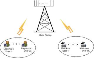
Figure 1: System model: the BS is equipped with $M$ antennas. The legitimate and malicious users have a single antenna each.

Consider the system model depicted in Fig. 1, where a BS estimates the uplink channels from $N_{L}$ LUs in the presence of $N_{M}$ MUs. The BS is equipped with $M$ antennas, while the MUs and LUs are each equipped with a single antenna. For facilitating channel separation in MMIMO system, $M$, $N_{L}$, and $N_{M}$ are required to satisfy $M\gg N_{M}+N_{L}$. The uplink and the corresponding downlink channels satisfy reciprocity. We perform channel separation to allow beamforming to individual users over the downlink channels. Assume that the channel separation process is performed within the coherent time of the channels. For $j=1,\ldots,N_{L}$ and $k=1,\ldots,N_{M}$, we use the $M\times 1$ vectors $\boldsymbol{h}_{j}$ and $\boldsymbol{g}_{k}$ to specify the channels from the $j$th LU and the $k$th MU to the BS, respectively. Whenever needed, $\beta_{1,j}$ and $\beta_{2,k}$ denote the path losses of channels of the $j$th LU and the $k$th MU, respectively. In the uplink, the $j$th LU and the $k$th MU send random symbols $A_{j}$ and $B_{k}$ to the BS, respectively. We allow $A_{1},\ldots,A_{N_{L}}$ and $B_{1},\ldots,B_{N_{M}}$ to follow any arbitrary distributions over any finite alphabets. The distributions of $B_{1},\ldots,B_{N_{M}}$ are likely to vary over instants. Note that since arbitrary symbol distributions are allowed, the proposed scheme will work for both pilot and data symbols. We assume that the distributions of $A_{1},\ldots,A_{N_{L}}$ are known to the MUs, while the distributions and even the alphabets of $B_{1},\ldots,B_{N_{M}}$ are, on the contrary, unknown to the BS and the LUs.

For $j=1,\ldots,N_{L}$ and $k=1,\ldots,N_{M}$, let us use $\mathcal{A}_{j}$ and $\mathcal{B}_{k}$ to denote alphabets of the $j$-th LU and the $k$-th MU, respectively. $\mathsf{a}_{j}$ and $\mathsf{b}_{k}$ denote the generic elements of $\mathcal{A}_{j}$ and $\mathcal{B}_{k}$, respectively. $P_{A_{j}}\left(\cdot\right)$ and $P_{B_{k}}\left(\cdot\right)$ are the distributions of $\mathcal{A}_{j}$ and $\mathcal{B}_{k}$, respectively. $P_{A_{1},\ldots,A_{N_{L}},B_{1},\ldots,B_{N_{M}}}\left(\cdot\right)$ denote joint distribution of $A_{1},\ldots,A_{N_{L}},B_{1},\ldots,B_{N_{M}}$. We assume in each instant, the joint distribution of $A_{1},\ldots,A_{N_{L}}$ and $B_{1},\ldots,B_{N_{M}}$ satisfies $P_{A_{1},\ldots,A_{N_{L}},B_{1},\ldots,B_{N_{M}}}\left(\mathsf{a}_{1},\ldots,\mathsf{a}_{N_{L}},\mathsf{b}_{1},\ldots,\mathsf{b}_{N_{M}}\right)>0$ whenever $P_{A_{1}}\left(\mathsf{a}_{1}\right)>0,\ldots P_{A_{N_{L}}}\left(\mathsf{a}_{N_{L}}\right)>0$, and $P_{B_{1}}\left(\mathsf{b}_{1}\right)>0,\ldots,P_{B_{N_{M}}}\left(\mathsf{b}_{N_{M}}\right)>0$. This assumption indicates $A_{1},\ldots,A_{N_{L}}$ and $B_{1},\ldots,B_{N_{M}}$ may be dependent with each other, but arbitrary $B_{k}$ cannot be exactly determined by other variables. In practice, it corresponds to the fact that the $k$th MU sends $B_{k}$ according to its overheard version of $A_{1},\ldots,A_{N_{L}}$. Nevertheless, the $k$th MU cannot get $A_{1},\ldots,A_{N_{L}}$ exactly because of the channel fading and noise.

The received symbol of the BS is specified by

$$\boldsymbol{y}=\boldsymbol{H}\boldsymbol{A}+\boldsymbol{G}\boldsymbol{B}+\boldsymbol{w},$$ (1)

where $\boldsymbol{w}$ is the noise vector, whose elements are i.i.d. circular-symmetric complex Gaussian (CSCG) random variables with zero mean and variance $\sigma^{2}$, and $\boldsymbol{H}=\left[\boldsymbol{h}_{1},\boldsymbol{h}_{2},\ldots,\boldsymbol{h}_{N_{L}}\right]$, $\boldsymbol{G}=\left[\boldsymbol{g}_{1},\boldsymbol{g}_{2},\ldots,\boldsymbol{g}_{N_{M}}\right]$, $\boldsymbol{A}=\left[A_{1},\ldots,A_{N_{L}}\right]^{T}$, and $\boldsymbol{B}=\left[B_{1},\ldots,B_{N_{M}}\right]^{T}$.

Assuming that the uplink channel described by (1) is used $n$ times within the coherent time of the channel, for the $i$th instant of use, (1) gives rise to

$$\boldsymbol{y}_{i}=\boldsymbol{H}\boldsymbol{A}_{i}+\boldsymbol{G}\boldsymbol{B}_{i}+\boldsymbol{w}_{i},$$ (2)

for $i=1,2,\ldots,n$, where $\boldsymbol{A}_{i}$ is $N_{L}\times 1$, and $\boldsymbol{B}_{i}$ is $N_{M}\times 1$. They are transmitted symbol vectors of the LUs and the MUs in the $i$th instant, respectively, and $\boldsymbol{w}_{i}$ is the noisy vector in the $i$th instant. Stacking the $n$ equations in (2) into a matrix form, we obtain

$$\mathbf{Y}=\left[\boldsymbol{H},\boldsymbol{G}\right]\left[\begin{array}[]{c}\mathbf{A}\\ \mathbf{B}\end{array}\right]+\mathbf{W}$$ (3)

where $\mathbf{Y}=\left[\boldsymbol{y}_{1},\boldsymbol{y}_{2},\ldots,\boldsymbol{y}_{n}\right]$, $\mathbf{W}=\left[\boldsymbol{w}_{1},\boldsymbol{w}_{2},\ldots,\boldsymbol{w}_{n}\right]$, $\mathbf{A}=\left[\boldsymbol{A}_{1},\boldsymbol{A}_{2},\ldots,\boldsymbol{A}_{n}\right]$, and $\mathbf{B}=\left[\boldsymbol{B}_{1},\boldsymbol{B}_{2},\ldots,\boldsymbol{B}_{n}\right]$. $\mathbf{A}$ and $\mathbf{B}$ are $N_{L}\times n$ and $N_{M}\times n$ matrices, respectively. In MMIMO systems, it is likely that the columns of $\left[\boldsymbol{H},\boldsymbol{G}\right]$ are linearly independent. We make this assumption throughout this paper. Note that linear independence is the only requirement that we impose on the channel vectors. Thus correlations among antenna elements are allowed.

The existence of $N_{M}$ MUs could be detected by attack detection schemes (see [17] for example). Focusing on channel separation, we assume the detection of MUs is perfect. Reiterating our attack model, $N_{M}$ and $N_{L}$ are known to the BS based on extensively research on attack detection techniques [7]–[19]. Following the existing works, we assume that each user has single antenna and the system works in TDD mode. Unlike the existing techniques, however, the BS does not know the exact distributions of $B_{1},\ldots,B_{N_{M}}$, $\left\{\beta_{1,1},\ldots\beta_{1,N_{L}}\right\}$, $\left\{\beta_{2,1},\ldots\beta_{2,N_{M}}\right\}$, $\boldsymbol{H}$, or $\boldsymbol{G}$ a priori. In this sense, our proposed channel separation is blind to the BS.

Let $\boldsymbol{S}$ be the $M\times(N_{L}+N_{M})$ signal subspace matrix whose columns form an orthonormal basis that spans the column space of $\left[\boldsymbol{H},\boldsymbol{G}\right]$. Then, we project $\mathbf{Y}$ onto the signal subspace and get from (3)

$$\mathbf{Z}=\frac{1}{\sqrt{M}}\boldsymbol{S}^{T}\mathbf{Y}=\left[\mathsf{\boldsymbol{Z}}^{\prime}_{1},\mathsf{\boldsymbol{Z}}^{\prime}_{2}\right]\left[\begin{array}[]{c}\mathbf{A}\\ \mathbf{B}\end{array}\right]+\mathbf{N}$$ (4)

where $\left[{\mathsf{\boldsymbol{Z}}}^{\prime}_{1},{\mathsf{\boldsymbol{Z}}}^{\prime}_{2}\right]=\frac{1}{\sqrt{M}}{\boldsymbol{S}}^{T}\left[\boldsymbol{H},\boldsymbol{G}\right]$, ${\mathsf{\boldsymbol{Z}}}^{\prime}_{1}=\left[{\mathsf{\boldsymbol{z}}}^{\prime}_{1,1},\ldots,{\mathsf{\boldsymbol{z}}}^{\prime}_{1,N_{L}}\right]$, ${\mathsf{\boldsymbol{Z}}}^{\prime}_{2}=\left[{\mathsf{\boldsymbol{z}}}^{\prime}_{2,1},\ldots,{\mathsf{\boldsymbol{z}}}^{\prime}_{2,N_{M}}\right]$, ${{\mathbf{N}}}=\frac{1}{\sqrt{M}}{\boldsymbol{S}}^{T}\mathbf{W}$, and the elements of ${{\mathbf{N}}}$ are i.i.d. Gaussian random variables with zero mean and variance $\frac{\sigma^{2}}{M}$. Clearly, ${{\mathbf{N}}}$ is independent of $\left[\mathsf{\boldsymbol{Z}}^{\prime}_{1},\mathsf{\boldsymbol{Z}}^{\prime}_{2}\right]\left[\begin{array}[]{c}\mathbf{A}\\ \mathbf{B}\end{array}\right]$. It is argued in [31] that this independence and the Gaussianity of ${{\mathbf{N}}}$ imply that

$$\left[\boldsymbol{\hat{H}},\boldsymbol{\hat{G}}\right]=\sqrt{M}\boldsymbol{S}\left[\mathsf{\boldsymbol{Z}}^{\prime}_{1},\mathsf{\boldsymbol{Z}}^{\prime}_{2}\right]$$ (5)

would be a reasonable estimator for the channel pair $\left[\boldsymbol{H},\boldsymbol{G}\right]$ if $\left[\mathsf{\boldsymbol{Z}}^{\prime}_{1},\mathsf{\boldsymbol{Z}}^{\prime}_{2}\right]$ could be found. In practice $\boldsymbol{S}$ is not known a priori, but can be estimated from the singular value decomposition $\mathbf{Y}=\boldsymbol{U}\boldsymbol{\varSigma}\boldsymbol{V}^{T}$ with orthogonal matrices $\boldsymbol{U}\in\mathbb{R}^{M\times M}$, $\boldsymbol{V}\in\mathbb{R}^{n\times n}$ and $M\times n$ diagonal singular value matrix $\boldsymbol{\varSigma}$. Then $\boldsymbol{S}$ can be well approximated by the first $(N_{L}+N_{M})$ left singular vectors in $\boldsymbol{U}$ when $M$ is large in the MMIMO system [31].

Incidentally, we can show that $\left[\mathsf{\boldsymbol{Z}}^{\prime}_{1},\mathsf{\boldsymbol{Z}}^{\prime}_{2}\right]$ cannot be uniquely determined from $\mathbf{Y}$ without additional authentication, or the knowledge of $\left\{\beta_{1,1},\ldots\beta_{1,N_{L}}\right\}$, $\left\{\beta_{2,1},\ldots\beta_{2,N_{M}}\right\}$, $\mathbf{A}$, and $\mathbf{B}$. Notice that when $\mathbf{A}$ and $\mathbf{B}$ have the same distribution in PSA, swapping the columns of $\left[\mathsf{\boldsymbol{Z}}^{\prime}_{1},\mathsf{\boldsymbol{Z}}^{\prime}_{2}\right]$ by observing $\mathbf{Z}$ in (4) would not change the distribution of $\mathbf{Z}$. Thus, it is impossible to obtain any decision rule among the permutations of the columns of $\left[\mathsf{\boldsymbol{Z}}^{\prime}_{1},\mathsf{\boldsymbol{Z}}^{\prime}_{2}\right]$.

As will be argued in the next section, it is however possible to separate channels in the sense of estimating $\left[\frac{\boldsymbol{h}_{1}}{|\boldsymbol{h}_{1}|},\ldots,\frac{\boldsymbol{h}_{N_{L}}}{|\boldsymbol{h}_{N_{L}}|},\frac{\boldsymbol{g}_{1}}{|\boldsymbol{g}_{1}|},\ldots,\frac{\boldsymbol{g}_{N_{M}}}{|\boldsymbol{g}_{N_{M}}|}\right]$ via (5), up to a permutation of the columns and a phase ambiguity on each column. Interchangeably, we also term the above-mentioned separation as channel direction separation, because the obtained $\left[\frac{\boldsymbol{h}_{1}}{|\boldsymbol{h}_{1}|},\ldots,\frac{\boldsymbol{h}_{N_{L}}}{|\boldsymbol{h}_{N_{L}}|},\frac{\boldsymbol{g}_{1}}{|\boldsymbol{g}_{1}|},\ldots,\frac{\boldsymbol{g}_{N_{M}}}{|\boldsymbol{g}_{N_{M}}|}\right]$ characterizes the channel directions of all users. As a result, we will be able to separate the downlink beamforming directions from the BS to the LUs and MUs based on channel reciprocity.

III Blind Channel Separation

First, notice that the columns of $\left[\mathsf{\boldsymbol{Z}}^{\prime}_{1},\mathsf{\boldsymbol{Z}}^{\prime}_{2}\right]\left[\begin{array}[]{c}\mathbf{A}\\ \mathbf{B}\end{array}\right]$ are $(N_{L}+N_{M})\times 1$ random vectors that range over the alphabet $\mathcal{Z}=\left\{\sum_{j=1}^{N_{L}}\mathsf{a}_{j}\mathsf{\boldsymbol{z}}^{\prime}_{1,j}+\sum_{k=1}^{N_{M}}\mathsf{b}_{k}\mathsf{\boldsymbol{z}}^{\prime}_{2,k}:\mathsf{a}_{j}\in\mathcal{A}_{j},\mathsf{b}_{k}\in\mathcal{B}_{k}\right\}$, where $\mathcal{A}_{j}$ and $\mathcal{B}_{k}$ are the respective alphabets of ${A}_{j}$ and ${B}_{k}$, for $j=1,\ldots,N_{L}$ and $k=1,\ldots,N_{M}$. The main idea of our channel separation scheme is to use $\mathcal{Z}$ to obtain $\left[\mathsf{\boldsymbol{Z}}^{\prime}_{1},\mathsf{\boldsymbol{Z}}^{\prime}_{2}\right]$ up to a column permutation, and then achieve the desired separation of channel directions via (5). In this section, we will first illustrate how to separate channels from perfect $\mathcal{Z}$, then propose estimation of $\mathcal{Z}$ based on received observations, finally give a method indicating channel separations from received observations step-by-step.

III-A Channel separation from perfect knowledge of $\mathcal{Z}$

For easy description of our proposed method, we give two definitions.

Definition 1.

For $\boldsymbol{v}\in\mathcal{Z}$, $\boldsymbol{v}^{\prime}\in\mathcal{Z}$, $\boldsymbol{v}\neq\boldsymbol{v}^{\prime}$, if one vector $\mathsf{\boldsymbol{z}}^{\prime}\notin\mathcal{Z}$ satisfies

$$\frac{\left(\boldsymbol{v}-\boldsymbol{v}^{\prime}\right)^{H}}{\left|\boldsymbol{v}-\boldsymbol{v}^{\prime}\right|\left|\mathsf{\boldsymbol{z}}^{\prime}\right|}\mathsf{\boldsymbol{z}}^{\prime}=\exp\left(\mathsf{i}\theta\right),$$ (6)

where $\theta$ could be arbitrary angle, we refer to this property as $\mathsf{\boldsymbol{z}}^{\prime}$ covers $\boldsymbol{v}$ and $\boldsymbol{v}^{\prime}$.

Definition 2.

For $\mathsf{\boldsymbol{z}}^{\prime}\neq 0$, $\mathsf{\boldsymbol{z}}^{\prime}\notin\mathcal{Z}$, subset $\mathcal{Z}_{s}\subset\mathcal{Z}$, if arbitrary $\boldsymbol{v}\in\mathcal{Z}_{s}$, $\forall\boldsymbol{v}^{\prime}\in\mathcal{Z}_{s}$ such that $\mathsf{\boldsymbol{z}}^{\prime}$ covers $\boldsymbol{v}$ and $\boldsymbol{v}^{\prime}$, we refer to this property as $\mathsf{\boldsymbol{z}}^{\prime}$ covers $\mathcal{Z}_{s}$ or $\mathsf{\boldsymbol{z}}^{\prime}$ covers $|\mathcal{Z}_{s}|$ points of $\mathcal{Z}$.

According to Definition 2, if $\mathsf{\boldsymbol{z}}^{\prime}$ covers $\mathcal{Z}_{s}$ and $\mathcal{Z}_{s}=\mathcal{Z}$, we term that as $\mathsf{\boldsymbol{z}}^{\prime}$ covers $\mathcal{Z}$.

Then, to explain how we may obtain $\left[\mathsf{\boldsymbol{Z}}^{\prime}_{1},\mathsf{\boldsymbol{Z}}^{\prime}_{2}\right]$ from $\mathcal{Z}$, let us start by considering an example with $N_{L}=N_{M}=1$ and both the LU and MU send BPSK symbols. That is, ${\mathsf{\boldsymbol{Z}}}^{\prime}_{1}=\left[{\mathsf{\boldsymbol{z}}}^{\prime}_{1,1}\right]$, ${\mathsf{\boldsymbol{Z}}}^{\prime}_{2}=\left[{\mathsf{\boldsymbol{z}}}^{\prime}_{2,1}\right]$, and $\mathcal{Z}=\left\{\underbrace{\mathsf{\boldsymbol{z}}^{\prime}_{1,1}+\mathsf{\boldsymbol{z}}^{\prime}_{2,1}}_{{\boldsymbol{v}}_{A}},\underbrace{-\mathsf{\boldsymbol{z}}^{\prime}_{1,1}+\mathsf{\boldsymbol{z}}^{\prime}_{2,1}}_{{\boldsymbol{v}}_{B}},\underbrace{\mathsf{\boldsymbol{z}}^{\prime}_{1,1}-\mathsf{\boldsymbol{z}}^{\prime}_{2,1}}_{{\boldsymbol{v}}_{C}},\underbrace{-\mathsf{\boldsymbol{z}}^{\prime}_{1,1}-\mathsf{\boldsymbol{z}}^{\prime}_{2,1}}_{{\boldsymbol{v}}_{D}}\right\}$.

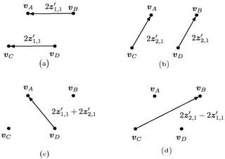
Figure 2: Subfigures (a) and (b) show that all points of $\mathcal{Z}$ lie on lines along the directions of $\mathsf{\boldsymbol{z}}^{\prime}_{1,1}$ and $\mathsf{\boldsymbol{z}}^{\prime}_{2,1}$, respectively. Subfigures (c) and (d) show that only two points in $\mathcal{Z}$ lie on lines along the directions of $\mathsf{\boldsymbol{z}}^{\prime}_{1,1}+\mathsf{\boldsymbol{z}}^{\prime}_{2,1}$ and $\mathsf{\boldsymbol{z}}^{\prime}_{2,1}-\mathsf{\boldsymbol{z}}^{\prime}_{1,1}$, respectively.

Then, it is clear that

$${\boldsymbol{v}}_{A}-{\boldsymbol{v}}_{B} =2\mathsf{\boldsymbol{z}}^{\prime}_{1,1},$$ (7)

$${\boldsymbol{v}}_{C}-{\boldsymbol{v}}_{D} =2\mathsf{\boldsymbol{z}}^{\prime}_{1,1}.$$ (8)

According to Definition 2, (7) and (8) jointly indicate that $\mathsf{\boldsymbol{z}}^{\prime}$ covers $\mathcal{Z}$. Similarly, it is easy to see that ${\boldsymbol{v}}_{A}-{\boldsymbol{v}}_{C}=2\mathsf{\boldsymbol{z}}^{\prime}_{2,1}$, ${\boldsymbol{v}}_{B}-{\boldsymbol{v}}_{D}=2\mathsf{\boldsymbol{z}}^{\prime}_{2,1}$, and hence $\mathsf{\boldsymbol{z}}^{\prime}_{2,1}$ also covers $\mathcal{Z}$. On the other hand, as long as $\mathsf{\boldsymbol{z}}^{\prime}_{1,1}$ and $\mathsf{\boldsymbol{z}}^{\prime}_{2,1}$ are linearly independent, we have that only ${\boldsymbol{v}}_{A}-{\boldsymbol{v}}_{D}=2\mathsf{\boldsymbol{z}}^{\prime}_{1,1}+2\mathsf{\boldsymbol{z}}^{\prime}_{2,1}$ and ${\boldsymbol{v}}_{B}-{\boldsymbol{v}}_{C}=2\mathsf{\boldsymbol{z}}^{\prime}_{2,1}-2\mathsf{\boldsymbol{z}}^{\prime}_{1,1}$. Thus, neither $\mathsf{\boldsymbol{z}}^{\prime}_{1,1}+\mathsf{\boldsymbol{z}}^{\prime}_{2,1}$ nor $\mathsf{\boldsymbol{z}}^{\prime}_{2,1}-\mathsf{\boldsymbol{z}}^{\prime}_{1,1}$ covers $\mathcal{Z}$. Note that the above cases exhaust the differences between all pairs of points in $\mathcal{Z}$. In summary, among all the pairwise differences, each of $\{\mathsf{\boldsymbol{z}}^{\prime}_{1,1},\mathsf{\boldsymbol{z}}^{\prime}_{2,1}\}$ covers $\mathcal{Z}$, but each of $\{\mathsf{\boldsymbol{z}}^{\prime}_{1,1}+\mathsf{\boldsymbol{z}}^{\prime}_{2,1},\mathsf{\boldsymbol{z}}^{\prime}_{2,1}-\mathsf{\boldsymbol{z}}^{\prime}_{1,1}\}$ does not. As a result, we may obtain $\mathsf{\boldsymbol{z}}^{\prime}_{1,1}$ and $\mathsf{\boldsymbol{z}}^{\prime}_{2,1}$ from $\mathcal{Z}$ by finding out all pairwise differences that cover $\mathcal{Z}$. It turns out that this observation extends to the general case as summarized in the proposition below:

Proposition 1.

Consider the general alphabet $\mathcal{Z}=\left\{\sum_{j=1}^{N_{L}}\mathsf{a}_{j}\mathsf{\boldsymbol{z}}^{\prime}_{1,j}+\sum_{k=1}^{N_{M}}\mathsf{b}_{k}\mathsf{\boldsymbol{z}}^{\prime}_{2,k}:\mathsf{a}_{j}\in\mathcal{A}_{j},\mathsf{b}_{k}\in\mathcal{B}_{k}\right\}$ where $\mathcal{A}_{j}$ and $\mathcal{B}_{k}$, for $j=1,\ldots,N_{L}$ and $k=1,\ldots,N_{M}$, are finite and with cardinalities at least $2$. As long as columns of $\{\mathsf{\boldsymbol{z}}^{\prime}_{1,1},\ldots,\mathsf{\boldsymbol{z}}^{\prime}_{1,N_{L}},\mathsf{\boldsymbol{z}}^{\prime}_{2,1},\ldots,\mathsf{\boldsymbol{z}}^{\prime}_{2,N_{M}}\}$ are linearly independent, every vector in $\left\{\mathsf{\boldsymbol{z}}^{\prime}_{1,1},\ldots,\mathsf{\boldsymbol{z}}^{\prime}_{1,N_{L}},\mathsf{\boldsymbol{z}}^{\prime}_{2,1},\ldots,\mathsf{\boldsymbol{z}}^{\prime}_{2,N_{M}}\right\}$ covers $\mathcal{Z}$. On the contrary, each vector of the form $\sum_{j=1}^{N_{L}}c_{1,j}\mathsf{\boldsymbol{z}}^{\prime}_{1,j}+\sum_{k=1}^{N_{M}}c_{2,k}\mathsf{\boldsymbol{z}}^{\prime}_{2,k}$, where at least two coefficients in $\left\{c_{1,1},\ldots,c_{1,N_{L}},c_{2,1},\ldots,c_{2,N_{M}}\right\}$ are nonzero, does not cover $\mathcal{Z}$.

Proof:

See the Appendix A. ∎

Notice that in massive MIMO system, columns of $\left[\boldsymbol{H},\boldsymbol{G}\right]$ are linearly independent in probability. It indicates that columns of $\{\mathsf{\boldsymbol{z}}^{\prime}_{1,1},\ldots,\mathsf{\boldsymbol{z}}^{\prime}_{1,N_{L}},\mathsf{\boldsymbol{z}}^{\prime}_{2,1},\ldots,\mathsf{\boldsymbol{z}}^{\prime}_{2,N_{M}}\}$ are almost always linearly independent.

Proposition 1 allows us to obtain the columns of $[\mathsf{\boldsymbol{Z}}^{\prime}_{1},\mathsf{\boldsymbol{Z}}^{\prime}_{2}]$ by finding all the pairwise differences of vectors in $\mathcal{Z}$ that covers $\mathcal{Z}$ itself. The steps given below show how Proposition 1 works on ${\mathcal{Z}}$. We use P1, P2 and P3 to label steps in this perfect case.

1. Let us write ${\mathcal{Z}}=\left\{\boldsymbol{v}_{1},\ldots,\boldsymbol{v}_{\left|\mathcal{Z}\right|}\right\}$, obtain the set of pairwise differences $\mathcal{D}=\big{\{}{\boldsymbol{v}}_{i}-{\boldsymbol{v}}_{j}:i<j\text{ and }i,j\in\{1,\ldots,|{\mathcal{Z}}|\}\big{\}}$.

2. Find subsets $\mathcal{D}^{*}$, $\mathcal{D}_{1}$, $\ldots$, $\mathcal{D}_{T}$, these subsets simultaneously satisfy following conditions.

   $$\mathcal{D}^{*}=\left\{\boldsymbol{d}_{1},\boldsymbol{d}_{2},\ldots,\boldsymbol{d}_{T}\right\}\subseteq\mathcal{D}$$

   $$\mathcal{D}_{t}=\left\{\boldsymbol{d}\in\mathcal{D}:\left|\frac{\boldsymbol{d}^{H}\boldsymbol{d}_{t}}{\big{|}\boldsymbol{d}\big{|}\big{|}\boldsymbol{d}_{t}\big{|}}-1\right|=0\right\},t=1,2\ldots,T$$

   $$\mathcal{D}=\bigcup_{t=1}^{T}\mathcal{D}_{t},\mathcal{D}_{s}\cap\mathcal{D}_{t}=\emptyset,s\neq t.$$

   Notice that $\mathcal{D}_{t}$ depends on $\boldsymbol{d}_{t}$. It is the $t$th element of $\mathcal{D}^{*}$. For each $t\in\{1,2,\ldots,T\}$, if ${\boldsymbol{v}}_{i}-{\boldsymbol{v}}_{j}\in\mathcal{D}_{t}$, then we collect ${\boldsymbol{v}}_{i}$ and ${\boldsymbol{v}}_{j}$ in ${\mathcal{Z}}_{t}$.

3. Define the weight of $\boldsymbol{d}_{t}$ as $W\left(\boldsymbol{d}_{t}\right)=\left|{\mathcal{Z}}_{t}\right|$. Use the $N_{L}+N_{M}$ vectors in $\mathcal{D}^{*}$ with the largest weights as estimates of the columns of $[\mathsf{\boldsymbol{Z}}^{\prime}_{1},\mathsf{\boldsymbol{Z}}^{\prime}_{2}]$.

In step P1, all pairwise differences of $\mathcal{Z}$ are obtained. Then, in step P2, we get ${\mathcal{Z}}_{1},\ldots,{\mathcal{Z}}_{T}$. They are covered by pairwise differences according to Definition 2. Finally, step P3 separates channels by finding $N_{L}+N_{M}$ vectors, each of which covers the most points. It exploits Proposition 1 that only pairwise differences along directions of channels could cover most points.

The above-mentioned steps are implemented for the perfect case that we have ${\mathcal{Z}}$. Let us go back to practical where ${\mathcal{Z}}$ is unknown. To separate channels, we need to to estimate ${\mathcal{Z}}$ from the observation $\mathbf{Y}$ given in (3), which will be discussed in next subsection.

III-B Estimation of $\mathcal{Z}$ based on $\mathbf{Y}$

To estimate $\mathcal{Z}$, we first consider the case that the columns of $\left[\mathsf{\boldsymbol{Z}}^{\prime}_{1},\mathsf{\boldsymbol{Z}}^{\prime}_{2}\right]\left[\begin{array}[]{c}\mathbf{A}\\ \mathbf{B}\end{array}\right]$ are i.i.d. vectors in order to introduce our method of estimating $\mathcal{Z}$. In Proposition 2, we will prove that the proposed method is also applicable to the case of non-i.i.d. columns. Further notice that the columns of $\mathbf{N}$ in (4) are i.i.d. random vectors that have the same distribution as that of the generic $(N_{M}+N_{L})\times 1$ random vector $\mathbf{n}$, whose elements are independent Gaussian random variables with zero mean and variance $\frac{\sigma^{2}}{M}$. If the columns of $\left[\mathsf{\boldsymbol{Z}}^{\prime}_{1},\mathsf{\boldsymbol{Z}}^{\prime}_{2}\right]\left[\begin{array}[]{c}\mathbf{A}\\ \mathbf{B}\end{array}\right]$ are i.i.d. random vectors that have the same distribution as the generic $(N_{M}+N_{L})\times 1$ random vector $\mathbf{{z}}^{\prime}$, then the columns of $\mathbf{Z}$, given in (4), are i.i.d. random vectors that have the same distribution as that of $\mathbf{z}=\mathbf{z}^{\prime}+\mathbf{n}$. Let $F_{\mathbf{z}}$, $F_{\mathbf{z}^{\prime}}$, and $F_{\mathbf{n}}$ denote the distributions of ${\mathbf{z}}$, ${\mathbf{z}^{\prime}}$, and ${\mathbf{n}}$, respectively. Then, because $\mathbf{z}^{\prime}$ and $\mathbf{n}$ are independent, we have

$$\Phi_{F_{\mathbf{z}}}(\boldsymbol{\omega})=\Phi_{F_{\mathbf{z}^{\prime}}}(\boldsymbol{\omega})\cdot\Phi_{F_{\mathbf{n}}}(\boldsymbol{\omega}).$$ (9)

where $\Phi_{F}(\boldsymbol{\omega})$ denotes the characteristic function of the distribution $F$, and $\boldsymbol{\omega}=[\omega_{1},\ldots,\omega_{2N_{L}+2N_{M}}]^{T}$ is the $(2N_{L}+2N_{M})\times 1$ frequency vector. Note that the noise variance parameter $\sigma^{2}$ is a characteristic of the receiver circuitry and can be measured a priori. We may assume that its value is known, and thus $\Phi_{F_{\mathbf{n}}}(\boldsymbol{\omega})=\exp\left\{-\frac{\sigma^{2}}{4M}\left|\boldsymbol{\omega}\right|^{2}\right\}$ is also known. On the other hand, $F_{\mathbf{z}}$ can be approximated by the empirical distribution of $\mathbf{Z}$ obtained directly from the observation $\mathbf{Y}$ as in (4). Hence the distribution $F_{\mathbf{z}^{\prime}}$ of $\mathbf{z}^{\prime}$ can be estimated using (9).

For ease of discussion, let us also use $\mathbf{z}$ to denote a generic column in the matrix $\mathbf{Z}$. To estimate $F_{\mathbf{z}^{\prime}}$ efficiently, we quantize ${\mathbf{z}}=[z_{1},\ldots,z_{N_{L}+N_{M}}]^{T}$ and use FFT to obtain the characteristic function of the quantized version of ${\mathbf{z}}$ as follows. Consider $m_{1}$ quantization levels $\mathsf{\widetilde{u}}_{1},\mathsf{\widetilde{u}}_{2},\ldots,\mathsf{\widetilde{u}}_{m_{1}}$, and the corresponding quantization intervals $\mathcal{B}\left(\mathsf{\widetilde{u}}_{1}\right),\mathcal{B}\left(\mathsf{\widetilde{u}}_{2}\right),\ldots,\mathcal{B}\left(\mathsf{\widetilde{u}}_{m_{1}}\right)$:

$$-\alpha_{1}=\mathsf{\widetilde{u}}_{1}<\mathsf{\widetilde{u}}_{2}<\mathsf{\widetilde{u}}_{3}<\cdots<\mathsf{\widetilde{u}}_{m_{1}-1}\leq\alpha_{1}=\mathsf{\widetilde{u}}_{m_{1}},$$

$$\mathcal{B}\left(\widetilde{\mathsf{u}}_{j}\right)=\begin{cases}\begin{array}[]{cc}\left(-\infty,\,\widetilde{\mathsf{u}}_{1}\right],&j=1\\ \left(\widetilde{\mathsf{u}}_{j-1},\,\widetilde{\mathsf{u}}_{j}\right],&j=2,3,\ldots,m_{1}-1\\ \left(\widetilde{\mathsf{u}}_{m_{1}-1},\,+\infty\right),&j=m_{1}\end{array}\end{cases}$$ (10)

where $\alpha_{1}>0$, $\widetilde{\mathsf{u}}_{j}-\widetilde{\mathsf{u}}_{j-1}=\delta_{1}$ for $j=2,3,\ldots,m_{1}$. Hence, we have $m_{1}=\left\lceil\frac{2\alpha_{1}}{\delta_{1}}\right\rceil+1$. The elements $z_{1},\ldots,z_{N_{L}+N_{M}}$ are respectively quantized to $\widetilde{z}_{1},\ldots,\widetilde{z}_{N_{L}+N_{M}}$ according to:

$$\widetilde{z}_{i}=\sum_{j=1}^{m_{1}}\widetilde{\mathsf{u}}_{j}\,\mathfrak{1}\left({\Re\left(z_{i}\right)\in\mathcal{B}\left(\widetilde{\mathsf{u}}_{j}\right)}\right)+\mathsf{i}\sum_{j=1}^{m_{1}}\widetilde{\mathsf{u}}_{j}\,\mathfrak{1}\left({\Im\left(z_{i}\right)\in\mathcal{B}\left(\widetilde{\mathsf{u}}_{j}\right)}\right),i=1,\ldots,N_{L}+N_{M},$$ (11)

where $\mathfrak{1}\left({\cdot}\right)$ denotes the indicator function. The quantized version of $\mathbf{z}$ is then $\widetilde{\mathbf{z}}=\left[\widetilde{z}_{1},\ldots,\widetilde{z}_{N_{L}+N_{M}}\right]^{T}$. Write $\widetilde{\mathcal{U}}=\left\{\mathsf{\widetilde{u}}_{1},\mathsf{\widetilde{u}}_{2},\ldots,\mathsf{\widetilde{u}}_{m_{1}}\right\}$, then the alphabet of $\widetilde{\mathbf{z}}$ is $\widetilde{\mathcal{U}}^{(N_{L}+N_{M})}\times\mathsf{i}\widetilde{\mathcal{U}}^{(N_{L}+N_{M})}$. We will denote it and enumerate its elements as $\widetilde{\mathcal{Z}}=\left\{\widetilde{\mathsf{\boldsymbol{u}}}_{1},\widetilde{\mathsf{\boldsymbol{u}}}_{2},\ldots,\mathsf{\widetilde{\boldsymbol{u}}}_{{m^{2N_{L}+2N_{M}}_{1}}}\right\}$.

Let $\widetilde{\mathbf{Z}}=\left[\widetilde{\mathbf{z}}_{1},\widetilde{\mathbf{z}}_{2},\ldots,\widetilde{\mathbf{z}}_{n}\right]$, where the $i$th column $\widetilde{\mathbf{z}}_{i}$ is the quantized version of the $i$th column of $\mathbf{Z}$. Next, obtain the empirical probability mass function (pmf) of the columns of $\widetilde{\mathbf{Z}}$ as

$$\triangle{F}_{\widetilde{\mathbf{z}}}\left(\widetilde{\mathsf{\boldsymbol{u}}}_{j}\right)=\frac{1}{n}\sum_{i=1}^{n}\mathfrak{1}\left({\widetilde{\mathbf{z}}_{i}=\widetilde{\mathsf{\boldsymbol{u}}}_{j}}\right)$$ (12)

for $j=1,2,\ldots,m^{2N_{L}+2N_{M}}_{1}$. Thus, the characteristic function of the empirical distribution $\triangle{F}_{\widetilde{\mathbf{z}}}$ is

$$\Phi_{\triangle{F}_{\widetilde{\mathbf{z}}}}\left(\boldsymbol{\omega}\right)=\sum_{j=1}^{m_{1}^{2N_{L}+2N_{M}}}\triangle{F}_{\widetilde{\mathbf{z}}}\left(\widetilde{\mathsf{\boldsymbol{u}}}_{j}\right)\exp\left\{-\mathsf{i}\left[\Re\left\{\widetilde{\mathsf{\boldsymbol{u}}}_{j}^{T}\right\},\Im\left\{\widetilde{\mathsf{\boldsymbol{u}}}_{j}^{T}\right\}\right]\boldsymbol{\omega}\right\}$$ (13)

where $\mathsf{i}=\sqrt{-1}$.

Similarly, let $\widetilde{\mathbf{Z}}^{\prime}=\left[\widetilde{\mathbf{z}}^{\prime}_{1},\widetilde{\mathbf{z}}^{\prime}_{2},\ldots,\widetilde{\mathbf{z}}^{\prime}_{n}\right]$, where the $i$th column $\widetilde{\mathbf{z}}^{\prime}_{i}$ is the quantized version of the $i$th column of $\left[\mathsf{\boldsymbol{Z}}^{\prime}_{1},\mathsf{\boldsymbol{Z}}^{\prime}_{2}\right]\left[\begin{array}[]{c}\mathbf{A}\\ \mathbf{B}\end{array}\right]$. To do this quantization step, we employ an extended quantization alphabet $\widetilde{\mathcal{Z}}^{\prime}=\left\{\widetilde{\mathsf{\boldsymbol{v}}}_{1},\widetilde{\mathsf{\boldsymbol{v}}}_{2},\ldots,\mathsf{\widetilde{\boldsymbol{v}}}_{{m^{(2N_{L}+2N_{M})}_{2}}}\right\}$, which is obtained by employing the same uniform quantization in (10) with $m_{2}$ quantization levels covering a range $\left(-\alpha_{2},\alpha_{2}\right)$. The length of each quantization duration is $\delta_{2}$. Hence, we have $m_{2}=\left\lceil\frac{2\alpha_{2}}{\delta_{2}}\right\rceil+1$. To facilitate analysis, we assume $\widetilde{\mathcal{Z}}^{\prime}$ is an extension of $\widetilde{\mathcal{Z}}$, i.e., $\widetilde{\mathcal{Z}}\subset\widetilde{\mathcal{Z}}^{\prime}$. Then, the empirical pmf of the columns of $\widetilde{\mathbf{Z}}^{\prime}$ is

$$\triangle{F}_{\widetilde{\mathbf{z}}^{\prime}}\left(\widetilde{\mathsf{\boldsymbol{v}}}_{j}\right)=\frac{1}{n}\sum_{i=1}^{n}\mathfrak{1}\left({\widetilde{\mathbf{z}}^{\prime}_{i}=\widetilde{\mathsf{\boldsymbol{v}}}_{j}}\right)$$ (14)

for $j=1,2,\ldots,m^{2N_{L}+2N_{M}}_{2}$.

Using $\Phi_{\triangle{F}_{\widetilde{\mathbf{z}}}}\left(\boldsymbol{\omega}\right)$ in place of $\Phi_{F_{\mathbf{z}}}\left(\boldsymbol{\omega}\right)$ and $\triangle{F}_{\widetilde{\mathbf{z}}^{\prime}}$ in place of ${F}_{\mathbf{z}^{\prime}}$ in (9), we obtain the estimator

$$\triangle\widehat{F}_{\widetilde{\mathbf{z}}^{\prime}}=\Phi^{-1}\left(\frac{\Phi_{\triangle{F}_{\widetilde{\mathbf{z}}}}\left(\boldsymbol{\omega}\right)}{\Phi_{F_{\mathbf{n}}}\left(\boldsymbol{\omega}\right)}\right)$$ (15)

for $\triangle{F}_{\widetilde{\mathbf{z}}^{\prime}}$, where $\Phi^{-1}$ denotes the inverse Fourier Transform with respect to (13). Note that the forward and inverse Fourier Transforms in (15) can be efficiently implemented using FFT and inverse FFT (IFFT), respectively. The asymptotic accuracy of this estimator is addressed by Proposition 2 below:

Proposition 2.

By choosing $n=\Omega\left(m_{2}^{2(N_{L}+N_{M})}\right)$, $m_{2}=\Omega\left(m_{1}^{3}\right)$, $\alpha_{1}=\alpha_{2}$, $2\alpha_{1}=(m_{1}-1)\delta_{1}$, $2\alpha_{2}=(m_{2}-1)\delta_{2}$, and $\frac{m_{2}-1}{m_{1}-1}$ is integer, there exists $\epsilon_{m_{2}}\rightarrow 0$ as $\alpha_{1}\rightarrow\infty$, $m_{2}\rightarrow\infty$, $\delta_{1}\rightarrow 0$, and $\delta_{2}\rightarrow 0$ such that whether $\mathbf{Z}$ is i.i.d. or non-i.i.d., as long as $\Re\left\{\mathcal{Z}\right\}\subseteq\left[-\alpha_{1},\alpha_{1}-\delta_{2}\right]^{N_{M}+N_{L}}$, $\Im\left\{\mathcal{Z}\right\}\subseteq\left[-\alpha_{1},\alpha_{1}-\delta_{2}\right]^{N_{M}+N_{L}}$, then the proposed estimator (15) has $\left|\triangle{F}_{\widetilde{\mathbf{z}}^{\prime}}\left(\widetilde{\boldsymbol{v}}_{j}\right)-\triangle\widehat{F}_{\widetilde{\mathbf{z}}^{\prime}}\left(\widetilde{\boldsymbol{v}}_{j}\right)\right|\leq\epsilon_{m_{2}}$ for $j=1,2,\ldots,m^{N_{L}+N_{M}}_{2}$.

Proof:

See the Appendix B. ∎

$\left[-\alpha_{1},\alpha_{1}-\delta_{2}\right]^{N_{M}+N_{L}}$ indicates Cartesian product of $\left[-\alpha_{1},\alpha_{1}-\delta_{2}\right]$ with ${N_{M}+N_{L}}$ times. The assumptions of $\Re\left\{\mathcal{Z}\right\}\subseteq\left[-\alpha_{1},\alpha_{1}-\delta_{2}\right]^{N_{M}+N_{L}}$ and $\Im\left\{\mathcal{Z}\right\}\subseteq\left[-\alpha_{1},\alpha_{1}-\delta_{2}\right]^{N_{M}+N_{L}}$ indicate that $\mathcal{Z}$ must be included in the quantization range. This could be achieved as $\alpha_{1}\rightarrow\infty$, while the transmitted power of MUs and LUs are not infinite.

Now, notice that $\mathcal{Z}$ is the support set of the empirical distribution, $\triangle{F}_{\mathbf{z}^{\prime}}$, of the columns of $\left[\mathsf{\boldsymbol{Z}}^{\prime}_{1},\mathsf{\boldsymbol{Z}}^{\prime}_{2}\right]\left[\begin{array}[]{c}\mathbf{A}\\ \mathbf{B}\end{array}\right]$. Clearly, as the quantization is fine enough, $\triangle{F}_{\widetilde{\mathbf{z}}^{\prime}}$ approximates $\triangle{F}_{\mathbf{z}^{\prime}}$ well. Thus, Proposition 2 tells us that we may use the essential support set

$$\widehat{\mathcal{Z}}=\left\{\widetilde{\boldsymbol{u}}\in\widetilde{\mathcal{Z}}:\triangle\widehat{F}_{\widetilde{\mathbf{z}}^{\prime}}\left(\widetilde{\boldsymbol{u}}\right)>\epsilon_{m_{2}}\right\}$$

of $\triangle\widehat{F}_{\widetilde{\mathbf{z}}^{\prime}}$ to estimate $\mathcal{Z}$.

It is worth noting that Proposition 2 does not require the columns of $\widetilde{\mathbf{Z}}^{\prime}$ to be i.i.d. random vectors as detailed in the proof. Thus, Proposition 2 extends the attack model to allow the MUs’ symbols to be arbitrary distributed, as discussed before.

Remark 1. Proposition 2 empowers our proposed method to be applicable even in the presence of the powerful MUs, who send symbol sequences following arbitrary unknown distribution. On contrast, some existing channel separation or estimation works based on maximum likelihood theory are no longer useful in the presence of the powerful MUs, since these works need to know the distributions of MUs’ symbols a priori.

Remark 2. In addition, we use only the support of $\triangle\widehat{F}_{\widetilde{\mathbf{z}}^{\prime}}$ to estimate $\mathcal{Z}$. Correlations between the columns of $\mathbf{Z}$ are immaterial to the proposed scheme. It indicates that our proposed scheme allows the symbols of MUs to statistically depend on the symbols of LUs. This property differs our work with ICA-based methods, which require symbols of MUs and LUs to be independent with each other.

III-C Blind channel separation method

According to Propositions 1 and 2, practical channel separation method could be achieved. In particular, Proposition 2 is used for estimating ${\mathcal{Z}}$. In other words, $\widehat{\mathcal{Z}}$ is obtained. Then, Proposition 1 achieves channel separation based on $\widehat{\mathcal{Z}}$.

Combining Propositions 1 and 2, we can obtain the following practical channel separation method:

1. Perform SVD on the observation matrix $\mathbf{Y}$, collect the first $N_{L}+N_{M}$ left singular vectors as columns of $\mathbf{S}$, and obtain $\mathbf{Z}=\frac{1}{\sqrt{M}}\mathbf{S}^{T}\mathbf{Y}$.

2. Quantize the columns of $\mathbf{Z}$ to obtain $\widetilde{\mathbf{Z}}=\left[\widetilde{\mathbf{z}}_{1},\widetilde{\mathbf{z}}_{2},\ldots,\widetilde{\mathbf{z}}_{n}\right]$, based on (11). Obtain the empirical pmf $\triangle{F}_{\widetilde{\mathbf{z}}}$ of the columns of $\widetilde{\mathbf{Z}}$ as described in (12).

3. Employ (15) to obtain $\triangle\widehat{F}_{\widetilde{\mathbf{z}}^{\prime}}$ via FFT and IFFT.

4. Choose a small $\epsilon>0$. Obtain the essential support set $\widehat{\mathcal{Z}}=\left\{\widetilde{\boldsymbol{u}}\in\widetilde{\mathcal{Z}}:\triangle\widehat{F}_{\widetilde{\mathbf{z}}^{\prime}}\left(\widetilde{\boldsymbol{u}}\right)>\epsilon\right\}$.

5. Write $\widehat{\mathcal{Z}}=\left\{\widehat{\boldsymbol{v}}_{1},\widehat{\boldsymbol{v}}_{2},\ldots,\widehat{\boldsymbol{v}}_{\left|\widehat{\mathcal{Z}}\right|}\right\}$. Obtain the set of pairwise differences $\mathcal{D}=\left\{\widehat{\boldsymbol{v}}_{i}-\widehat{\boldsymbol{v}}_{j}:i<j\text{ and }i,j\in\{1,\ldots,|\widehat{\mathcal{Z}}|\}\right\}$.

6. Choose a small $\gamma>0$. Find subsets $\mathcal{D}^{*}$, $\mathcal{D}_{1}$, $\ldots$, $\mathcal{D}_{T}$, these subsets simultaneously satisfy following conditions.

   $$\mathcal{D}^{*}=\left\{\boldsymbol{d}_{1},\boldsymbol{d}_{2},\ldots,\boldsymbol{d}_{T}\right\}\subseteq\mathcal{D}$$

   $$\mathcal{D}_{t}=\left\{\boldsymbol{d}\in\mathcal{D}:\left|\frac{\boldsymbol{d}^{H}\boldsymbol{d}_{t}}{\big{|}\boldsymbol{d}\big{|}\big{|}\boldsymbol{d}_{t}\big{|}}-1\right|\leq\gamma\right\},t=1,2\ldots,T$$

   $$\mathcal{D}=\bigcup_{t=1}^{T}\mathcal{D}_{t},\mathcal{D}_{s}\cap\mathcal{D}_{t}=\emptyset,s\neq t.$$

   Notice that $\mathcal{D}_{t}$ depends on $\boldsymbol{d}_{t}$. It is the $t$th element of $\mathcal{D}^{*}$. Algorithm 1 is gave for illustrating how to find such $\mathcal{D}_{1},\mathcal{D}_{2},\ldots,\mathcal{D}_{T}$, and $\mathcal{D}^{*}$. For each $t\in\{1,2,\ldots,T\}$, if $\widehat{\boldsymbol{v}}_{i}-\widehat{\boldsymbol{v}}_{j}\in\mathcal{D}_{t}$, then we collect $\widehat{\boldsymbol{v}}_{i}$ and $\widehat{\boldsymbol{v}}_{j}$ in $\widehat{\mathcal{Z}}_{t}$. Algorithm 1 illustrates how to implement this step.

7. Define the weight of $\boldsymbol{d}_{t}$ as $W\left(\boldsymbol{d}_{t}\right)=\sum_{\widehat{\boldsymbol{v}}\in\widehat{\mathcal{Z}}_{t}}\triangle\widehat{F}_{\widetilde{\mathbf{z}}^{\prime}}\left(\widehat{\boldsymbol{v}}\right)$. Use the $N_{L}+N_{M}$ vectors in $\mathcal{D}^{*}$ with the largest weights as estimates of the columns of $[\mathsf{\boldsymbol{Z}}^{\prime}_{1},\mathsf{\boldsymbol{Z}}^{\prime}_{2}]$.

8. Employ (5) to estimate $\left[\frac{\boldsymbol{h}_{1}}{|\boldsymbol{h}_{1}|},\ldots,\frac{\boldsymbol{h}_{N_{L}}}{|\boldsymbol{h}_{N_{L}}|},\frac{\boldsymbol{g}_{1}}{|\boldsymbol{g}_{1}|},\ldots,\frac{\boldsymbol{g}_{N_{M}}}{|\boldsymbol{g}_{N_{M}}|}\right]$ up to a permutation of the columns and up to a phase ambiguity on each column, from the estimated $[\mathsf{\boldsymbol{Z}}^{\prime}_{1},\mathsf{\boldsymbol{Z}}^{\prime}_{2}]$ obtained in 7).

Steps 1)-4) are designed to obtain the estimator in (15), and the estimation of ${\mathcal{Z}}$. The performance of steps 1)-4) is guaranteed by Proposition 2. Steps 5)-7) are obtained by respectively modifying steps P1-P3 a little bit. Compared to steps P1-P3, in step 5), $\mathcal{D}$ is obtained from $\widehat{\mathcal{Z}}$ rather than ${\mathcal{Z}}$. Note that we use $\widehat{\mathcal{Z}}$ to approximate ${\mathcal{Z}}$ for practical application. $\widehat{\mathcal{Z}}$ often contains many more points than $\mathcal{Z}$ as shown in Fig. 3. To solve this problem, step 6) first clusters all pairwise differences by defining $\mathcal{D}_{t}=\left\{\boldsymbol{d}\in\mathcal{D}:\left|\frac{\boldsymbol{d}^{H}\boldsymbol{d}_{t}}{\big{|}\boldsymbol{d}\big{|}\big{|}\boldsymbol{d}_{t}\big{|}}-1\right|\leq\gamma\right\}$. Step  7) uses a likelihood metric to approximately obtain the set of covering pairwise difference vectors among the clusters obtained in step 6).

Algorithm 1 Achieving $\widehat{\mathcal{Z}}_{1},\widehat{\mathcal{Z}}_{2},\ldots,\widehat{\mathcal{Z}}_{T}$ by step 6)

1:  $\mathcal{D}=\left\{\boldsymbol{d}^{\prime}_{1},\boldsymbol{d}^{\prime}_{2}\ldots\boldsymbol{d}^{\prime}_{\left|\mathcal{D}\right|}\right\}$, $\widehat{\mathcal{Z}}=\left\{\widehat{\boldsymbol{v}}_{1},\widehat{\boldsymbol{v}}_{2},\ldots,\widehat{\boldsymbol{v}}_{\left|\widehat{\mathcal{Z}}\right|}\right\}$, $t=1$.

2:  $\boldsymbol{d}_{1}=\boldsymbol{d}^{\prime}_{1}$, $\mathcal{D}^{*}=\left\{\boldsymbol{d}_{1}\right\}$.

3:  while $\mathcal{D}\neq\emptyset$ do

4:     $\mathcal{D}_{t}=\emptyset$, $\widehat{\mathcal{Z}}_{t}=\emptyset$

5:     for $j=1$ to $\left|\mathcal{D}\right|$ do

6:        if $\left|\frac{\boldsymbol{d}^{\prime H}_{j}\boldsymbol{d}_{t}}{\big{|}\boldsymbol{d}^{\prime H}_{j}\big{|}\big{|}\boldsymbol{d}_{t}\big{|}}-1\right|\leq\gamma$ then

7:           $\mathcal{D}_{t}\impliedby\boldsymbol{d}^{\prime}_{j}$

8:        end if

9:        $j\leftarrow j+1$

10:     end for

11:     for $i=1$ to $\left|\widehat{\mathcal{Z}}\right|$ do

12:        for $k=i+1$ to $\left|\widehat{\mathcal{Z}}\right|$ do

13:           if  $\widehat{\boldsymbol{v}}_{i}-\widehat{\boldsymbol{v}}_{k}\in\mathcal{D}_{t}$ then

14:              $\widehat{\mathcal{Z}}_{t}\impliedby\widehat{\boldsymbol{v}}_{i}$, $\widehat{\mathcal{Z}}_{t}\impliedby\widehat{\boldsymbol{v}}_{k}$

15:           end if

16:           $k\leftarrow k+1$

17:        end for

18:        $i\leftarrow i+1$

19:     end for

20:     $\mathcal{D}\leftarrow\mathcal{D}-\mathcal{D}_{t}$, $\mathcal{D}=\left\{\boldsymbol{d}^{\prime}_{1},\boldsymbol{d}^{\prime}_{2}\ldots\boldsymbol{d}^{\prime}_{\left|\mathcal{D}\right|}\right\}$,$t\leftarrow t+1$, $\boldsymbol{d}_{t}=\boldsymbol{d}^{\prime}_{1}$, $\mathcal{D}^{*}\impliedby\left\{\boldsymbol{d}^{\prime}_{1}\right\}$.

21:  end while

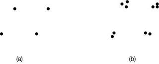
Figure 3: An example of comparison between ${\mathcal{Z}}$ and $\widehat{\mathcal{Z}}$. They are illustrated in subfigures (a) and (b), respectively.

Remark 3 The proposed method obtains partial CSI. Comparing with full CSI, i.e., $\left[\boldsymbol{H},\boldsymbol{G}\right]$, the obtained result still has the permutation of columns and the phase ambiguity in each column. This observation is similar to some blind source separation methods (e.g., ICA), and needs further processing to obtain full CSI. Nevertheless, unlike the existing methods, it is clear that the proposed method does not require the a priori knowledge of $\mathcal{Z}$ or the symbol alphabets of the LUs and MUs, and thus imposes no restriction on the statistic dependence between symbols of the LUs and MUs.

III-D Complexity analysis

We proceed to briefly analyze the computational complexity of the blind channel separation method described in Section III-C as follows:

1. The SVD operations, which has a complexity $\mathcal{O}\left(\max\{M^{2}n,n^{3}\}\right)$, dominates in step 1).

2. Quantizing the columns of $\boldsymbol{Z}$ and obtaining $\triangle{F}_{\widetilde{\mathbf{z}}}$ require $\mathcal{O}\left(nMm_{1}\right)$ complexity in step 2).

3. The FFT (and IFFT) operations in step 3) perform $(N_{L}+N_{M})$-dimensional $m_{2}$-point FFT. Hence the complexity of step 3) is $\mathcal{O}\left(\left(N_{L}+N_{M}\right)m_{2}^{\left(N_{L}+N_{M}\right)}\log m_{2}\right)$.

4. Notice that $\left|\mathcal{Z}\right|=\prod_{i=1}^{N_{L}}\left|\mathcal{A}_{i}\right|\prod_{j=1}^{N_{M}}\left|\mathcal{B}_{j}\right|$. By Proposition 2, $\left|\widehat{\mathcal{Z}}\right|\approx\left|\mathcal{Z}\right|$ for large $m_{2}$ and $n$. In addition, $T\leq\left|\mathcal{D}\right|\leq\left|\widehat{\mathcal{Z}}\right|^{2}\approx\left|\mathcal{Z}\right|^{2}$. Hence, the complexity of steps 4)–7) can be approximately upper bounded by $\mathcal{O}\left(\left(N_{L}+N_{M}\right)\left(\prod_{i=1}^{N_{L}}\left|\mathcal{A}_{i}\right|\prod_{j=1}^{N_{M}}\left|\mathcal{B}_{j}\right|\right)^{3}\right)$.

Recall that $m_{2}=\Omega(m^{3}_{1})$ and we would often choose a large $m_{2}$ that gives $\left(\prod_{i=1}^{N_{L}}\left|\mathcal{A}_{i}\right|\prod_{j=1}^{N_{M}}\left|\mathcal{B}_{j}\right|\right)^{3}\leq m_{2}^{\left(N_{L}+N_{M}\right)}\log m_{2}$. Therefore, the total complexity of the blind channel separation method can be characterized by

$$\mathcal{O}\left(\max\{M^{2}n,n^{3}\}\right)+\mathcal{O}\left(nMm_{2}\right)+\mathcal{O}\left(\left(N_{L}+N_{M}\right)m_{2}^{\left(N_{L}+N_{M}\right)}\log m_{2}\right).$$

Notice that the computation complexity of the proposed method is higher than the existing methods. For example, the complexity of FastICA is no more than $\mathcal{O}\left(\max\{M^{2}n,n^{3}\}\right)+\mathcal{O}\left(nM^{2}m_{2}\right)$[32, 33]. Nevertheless, ICA methods require the a priori knowledge of $\mathcal{Z}$ and statistic independence between symbols of the LUs and MUs, while the proposed method does not require that. In other words, the proposed method imposes less restrictions on MUs at cost of its computation complexity. In that sense, the proposed method may be more suitable to combat against the MUs whose misbehavior is out of the control of the BS, as long as the computation capability of the BS is sufficient.

IV Performance Evaluation

In this section, we present our simulation results to evaluate the performance of the blind channel separation (BCS) method described in Section III-C. In the simulation, we generate $100,000$ instances of the channel vectors based on the block Rayleigh fading model. That is, the elements of each column in $\boldsymbol{H}$ and $\boldsymbol{G}$ are chosen as i.i.d. CSCG random variables with mean $0$ mean and variance $1$. We then average performance metric, given later, over $100,000$ channel realizations. We choose $\alpha_{1}=\alpha_{2}$ and $m_{1}=m_{2}=64$. We consider the antenna array sizes of $M=64$ and $M=128$, and two different numbers of observation instances, namely, $n=300$ and $n=500$, respectively. Each LU sends symbols with power of $P_{s}$. The ratio $\frac{P_{s}}{\sigma^{2}}$ is the per-antenna signal-to-noise ratio (SNR) of the LU’s signal. We vary the SNR value in the simulation to evaluate the channel separation performance of the proposed method.

IV-A Performance metric

Let $\boldsymbol{h}$ be a column of $\left[\boldsymbol{H},\boldsymbol{G}\right]$, and $\mathbf{P}_{\boldsymbol{h}}=\frac{\boldsymbol{h}\boldsymbol{h}^{H}}{\left|\boldsymbol{h}\right|^{2}}$ be the projection on the subspace spanned by $\boldsymbol{h}$. Consider the $j$th legitimate user. Suppose that $\boldsymbol{d}$ is an uplink channel direction vector from this user to the BS obtained by some channel estimation algorithm. By reciprocity, downlink beamforming is performed based on $\boldsymbol{d}$. Then, $|\mathbf{P}_{\boldsymbol{h}_{j}}\boldsymbol{d}|^{2}$ is the power directed to the $j$th legitimate user by the BS. On the other hand, the total power leaked to other legitimate users and malicious users is given by $\sum_{l=1,l\neq j}^{N_{L}}|\mathbf{P}_{\boldsymbol{h}_{l}}\boldsymbol{d}|^{2}+\sum_{k=1}^{N_{M}}|\mathbf{P}_{\boldsymbol{g}_{k}}\boldsymbol{d}|^{2}$. Hence, the directed-to-leakage power ratio (DLPR)

$$\frac{|\mathbf{P}_{\boldsymbol{h}_{j}}\boldsymbol{d}|^{2}}{\sum_{l=1,l\neq j}^{N_{L}}|\mathbf{P}_{\boldsymbol{h}_{l}}\boldsymbol{d}|^{2}+\sum_{k=1}^{N_{M}}|\mathbf{P}_{\boldsymbol{g}_{k}}\boldsymbol{d}|^{2}}$$ (16)

measures the ratio of the power directed to the $j$th legitimate user to the power leaked to all others if $\boldsymbol{d}$ is employed to perform beamforming based on channel reciprocity. Clearly, substituting $\boldsymbol{d}=\frac{\boldsymbol{h}_{j}}{\left|\boldsymbol{h}_{j}\right|}$ in (16) obtains the DLPR value when the channel direction estimation is perfect.

Now, let $\widehat{\boldsymbol{H}}=\left[\widehat{\boldsymbol{h}}_{1},\ldots,\widehat{\boldsymbol{h}}_{N_{L}+N_{M}}\right]$ be the channel direction vectors estimated using the blind channel separation scheme described in Section III-C. Since we do not know which column of $\widehat{\boldsymbol{H}}$ corresponds to $\boldsymbol{h}_{j}$, we consider the maximum among the DLPRs of all the possibilities:

$$\text{DLPR}_{j}(\boldsymbol{H},\boldsymbol{G})\triangleq\max_{i\in\{1,2,\ldots,N_{L}+N_{M}\}}\frac{|\mathbf{P}_{\boldsymbol{h}_{j}}\widehat{\boldsymbol{h}}_{i}|^{2}}{\sum_{l=1,l\neq j}^{N_{L}}|\mathbf{P}_{\boldsymbol{h}_{l}}\widehat{\boldsymbol{h}}_{i}|^{2}+\sum_{k=1}^{N_{M}}|\mathbf{P}_{\boldsymbol{g}_{k}}\widehat{\boldsymbol{h}}_{i}|^{2}}.$$

Finally, we conservatively use the worst-case DLPR among all the legitimate users as our performance metric:

$$\text{DLPR}(\boldsymbol{H},\boldsymbol{G})\triangleq\min_{j\in\{1,2,\ldots,N_{L}\}}\text{DLPR}_{j}(\boldsymbol{H},\boldsymbol{G}).$$ (17)

Note that the DLPR in (17) is a function of the channel vectors $[\boldsymbol{H},\boldsymbol{G}]$.

IV-B Simulation

We first consider a PSA scenario with two LUs and one MU. The MU conducts PSA by sending equally likely random BPSK symbols as those of LUs. The BPSK symbols of all these three users are independent with each other. We simulate DLPR achieved by perfect CSI, our proposed BCS scheme, and traditional ICA [32], respectively. The length of observations is set to $n=300$. Two array sizes of $M=128$ and $M=64$ are considered. Fig. 4 shows the obtained result. Notice that it is a standard scenario for ICA since all users send independent symbols. We observe from Fig. 4 that our proposed BCS outperforms ICA, and achieves near-optimal performance. The performance improvement is coursed by the fact that our proposed BCS attempts to cut down the impact of noise. In particular, revisiting (9), our proposed BCS estimates distribution of desired signals (i.e., $\left[\mathsf{\boldsymbol{Z}}^{\prime}_{1},\mathsf{\boldsymbol{Z}}^{\prime}_{2}\right]\left[\begin{array}[]{c}\mathbf{A}\\ \mathbf{B}\end{array}\right]$) by removing CF of noise from CF of received noisy observations (i.e., $\boldsymbol{Y}$). On the other hand, ICA is derived for desired signals without any noise, and then applied to the noisy observations straightforwardly.

Then, we consider a PJA scenario with two LUs and one MU. The LUs send equally likely random BPSK symbols, while the MU conducts PJA by sending PAM symbols according to its wiretapped signal from the LUs. In particular, $P_{B_{1}|A_{1}}(+3|+1)=P_{B_{1}|A_{1}}(-1|+1)=\frac{1}{3}$, $P_{B_{1}|A_{1}}(+1|+1)=P_{B_{1}|A_{1}}(-3|+1)=\frac{1}{6}$, $P_{B_{1}|A_{1}}(+1|-1)=P_{B_{1}|A_{1}}(+3|-1)=\frac{1}{6}$, $P_{B_{1}|A_{1}}(-1|-1)=P_{B_{1}|A_{1}}(-3|-1)=\frac{1}{3}$, where $P_{B_{1}|A_{1}}$ denotes the conditional probability of symbol of the MU given symbol sent by the first LU. The length of observations is set to $n=800$. We observe from the Fig. 5 that for $M=64$ and $M=128$, the proposed method achieves DLPR close to that achieved by perfect CSI within $1$dB. In contrast, even the per-antenna SNR reaches $16$dB, the DLPR achieved by the traditional ICA scheme is only about 50% of that achieved by the scheme with perfect CSI. This performance gap is brought by the fact that ICA requires independence between symbols sent by users. In this scenario, the dependence between symbols of these three users degrades the performance. Our proposed BCS works based on alphabet estimation, imposing no restrict on statistic dependence between symbols of users. Therefore, our proposed BCS outperforms ICA.

Finally, we simulate another PJA scenario with two LUs and two MUs. The MUs employ non-stationary PAM attack. In particular, in odd instants, they send random symbols following statistic distribution $P_{B_{1}}(+3)=P_{B_{2}}(+3)=\frac{1}{3}$, $P_{B_{1}}(-1)=P_{B_{2}}(-1)=\frac{2}{3}$. In even instants, they send random symbols following statistic distribution $P_{B_{1}}(+1)=P_{B_{2}}(+1)=\frac{2}{3}$, $P_{B_{1}}(-1)=P_{B_{2}}(-1)=\frac{1}{3}$. As shown in Fig. 6, for $M=64$ and $M=128$, our proposed BCS still outperforms traditional ICA. ICA separates channels by minimizing a contrast function that measure gaussianity of its output. Its employed contrast function may be not always suitable for the non-stationary attack. As a result, the performance is degraded. On the contrast, Proposition 2 guarantees our proposed BCS is still available to non-stationary attack.

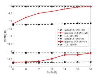
Figure 4: DLPR performance under PSA scenario with $N_{L}=2$, $N_{M}=1$, and all users send BPSK symbols.

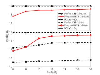
Figure 5: DLPR performance under PJA scenario where the malicious user sends symbols correlated to those of legitimate users.

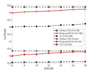
Figure 6: DLPR performance under PJA scenario where the malicious user sends symbols according to varying distribution.

All the above results demonstrate that the proposed BCS method is effective in separating and estimating the channel directions of the LU and the MU. With our proposed method, if the MUs conduct attack, the attack signals will expose the MUs’ channel directions. Then, forced by our proposed method, the MUs may have to keep silent, such that the BS cannot estimate their channel vectors. Nevertheless, in such case, without interference of the MUs, the BS can get the CSI of the LUs. As a result, the BS is able to focus its power along the direction of the LUs, while the leakage to the MUs is little due to quasi-orthogonality of the channel vectors in MMIMO system. In summary, the MUs cannot achieve its goal of eavesdropping the downlink information. As a beneficial result, the security of the system is guaranteed.

V Conclusions

We have proposed a BCS method to differentiate the channel directions from the LU and MU to the BS in the uplink of a MMIMO system. With channel reciprocity, the BS is able to use the channel directions to steer the beam toward the LUs and MUs separately with minimal power and information leakage, and further verify their identities by use of some higher layer authentication protocols. Simulation results have shown that the proposed method can achieve good channel separation performance in terms of achieving good DLPR performance at low to moderate per-antenna SNR and near-perfect DLPR performance at high SNR. It is also noted that even when the MUs are allowed to impersonate the LUs by sending symbols of distribution identical to that of the LUs’ symbols, the proposed scheme still works very well. Moreover, the proposed method does not requires the BS to have any partial CSI of the channels a priori. The complexity of the method is polynomial in the number of antennas and the number of observation instants, but is exponential in the number of users. Thus the method is most suitable for the practical use when the number of users is small. As an extension to the current work, it is interesting to investigate wheatear the knowledge of the LUs’ symbols (such as pilot symbols) can be utilized to reduce the complexity of the channel separation method.

Appendix A Proof of Proposition 1

Proof:

Let $\mathcal{A}_{j}=\left\{\mathsf{a}_{j,1},\ldots,\mathsf{a}_{j,\left|\mathcal{A}_{j}\right|}\right\}$ and $\mathcal{B}_{k}=\left\{\mathsf{b}_{k,1},\ldots,\mathsf{b}_{k,\left|\mathcal{B}_{k}\right|}\right\}$. Without loss of generalization, we focus on the direction of $\mathsf{\boldsymbol{z}}^{\prime}_{1,j}$. For an arbitrary point $\boldsymbol{u}$ in $\mathcal{Z}$, we may write it as $\boldsymbol{u}=\mathsf{a}_{j,s}\mathsf{\boldsymbol{z}}^{\prime}_{1,j}+\mathsf{\boldsymbol{z}}^{\prime}$, for some $s\in\{1,\ldots,\left|\mathcal{A}_{j}\right|\}$, and $\mathsf{\boldsymbol{z}}^{\prime}=\sum_{j^{\prime}=1,j\neq j^{\prime}}^{N_{L}}\mathsf{a}_{j^{\prime}}\mathsf{\boldsymbol{z}}^{\prime}_{1,j^{\prime}}+\sum_{k=1}^{N_{M}}\mathsf{b}_{k}\mathsf{\boldsymbol{z}}^{\prime}_{2,k}$. Then there must exist another point $\boldsymbol{u}^{\prime}\in\mathcal{Z}$ satisfying $\boldsymbol{u}^{\prime}=\mathsf{a}_{j,s^{\prime}}\mathsf{\boldsymbol{z}}^{\prime}_{1,1}+\mathsf{\boldsymbol{z}}^{\prime}$ with some $s^{\prime}\neq s$. Because the difference

$$\boldsymbol{u}^{\prime}-\boldsymbol{u}=(\mathsf{a}_{j,s^{\prime}}-\mathsf{a}_{j,s})\mathsf{\boldsymbol{z}}^{\prime}_{1,j},$$

$\boldsymbol{u}$ and $\boldsymbol{u}^{\prime}$ are covered by $\mathsf{\boldsymbol{z}}^{\prime}_{1,j}$ according to Definition 1. It is obvious that this same argument applies to every point in $\mathcal{Z}$ and every direction in $\left\{\mathsf{\boldsymbol{z}}^{\prime}_{1,1},\ldots,\mathsf{\boldsymbol{z}}^{\prime}_{1,N_{L}},\mathsf{\boldsymbol{z}}^{\prime}_{2,1},\ldots,\mathsf{\boldsymbol{z}}^{\prime}_{2,N_{M}}\right\}$. Hence, every vector in $\left\{\mathsf{\boldsymbol{z}}^{\prime}_{1,1},\ldots,\mathsf{\boldsymbol{z}}^{\prime}_{1,N_{L}},\mathsf{\boldsymbol{z}}^{\prime}_{2,1},\ldots,\mathsf{\boldsymbol{z}}^{\prime}_{2,N_{M}}\right\}$ covers $\mathcal{Z}$.

Furthermore, without loss of generalization, consider the vector $c_{1,j}\mathsf{\boldsymbol{z}}^{\prime}_{1,j}+c_{2,k}\mathsf{\boldsymbol{z}}^{\prime}_{2,k}$. Focus on the point

$$\boldsymbol{v}=\mathsf{a}_{j,\hat{s}}\mathsf{\boldsymbol{z}}^{\prime}_{1,j}+\mathsf{b}_{k,\hat{t}}\mathsf{\boldsymbol{z}}^{\prime}_{2,k}+\bar{\mathsf{\boldsymbol{z}}}^{\prime}\in\mathcal{Z}$$

where $\bar{\mathsf{\boldsymbol{z}}}^{\prime}=\sum_{j^{\prime}=1,j\neq j}^{N_{L}}\mathsf{a}_{j^{\prime}}\mathsf{\boldsymbol{z}}^{\prime}_{1,j^{\prime}}+\sum_{k^{\prime}=1,k^{\prime}\neq k}^{N_{M}}\mathsf{b}_{k^{\prime}}\mathsf{\boldsymbol{z}}^{\prime}_{2,k^{\prime}}$. $\mathsf{a}_{j,\hat{s}}$ and $\mathsf{b}_{k,\hat{t}}$ are chosen according to $\hat{s}=\underset{s\in\mathcal{S}}{\arg}\min\Im\left\{\frac{c_{2}}{c_{1}}\mathsf{a}_{j,s}\right\}$, where $\mathcal{S}=\left\{s:\arg\min_{s\in\left\{1,2,\ldots,\left|\mathcal{A}_{j}\right|\right\}}\Re\left\{\frac{c_{2}}{c_{1}}\mathsf{a}_{j,s}\right\}\right\}$ and

$$\hat{t}=\underset{t\in\mathcal{T}}{\arg}\max\Im\left\{\mathsf{b}_{k,t}\right\}.$$

where $\mathcal{T}=\left\{t:{\arg\max}_{t\in\left\{1,2,\ldots,\left|\mathcal{B}_{k}\right|\right\}}\Re\left\{\mathsf{b}_{k,t}\right\}\right\}$.

If there were a different $\boldsymbol{v}^{\prime}\in\mathcal{Z}$ such that $\boldsymbol{v}^{\prime}$ and $\boldsymbol{v}$ are covered by $c_{1,j}\mathsf{\boldsymbol{z}}^{\prime}_{1,j}+c_{2,k}\mathsf{\boldsymbol{z}}^{\prime}_{2,k}$, notice that columns of $\{\mathsf{\boldsymbol{z}}^{\prime}_{1,1},\ldots,\mathsf{\boldsymbol{z}}^{\prime}_{1,N_{L}}\mathsf{\boldsymbol{z}}^{\prime}_{2,1},\ldots,\mathsf{\boldsymbol{z}}^{\prime}_{2,N_{M}}\}$ are linearly independent, then $\boldsymbol{v}^{\prime}$ could be rewritten as $\boldsymbol{v}^{\prime}=\mathsf{a}^{\prime}_{j,s}\mathsf{\boldsymbol{z}}^{\prime}_{1,j}+\mathsf{b}^{\prime}_{k,t}\mathsf{\boldsymbol{z}}^{\prime}_{2,k}+\bar{\mathsf{\boldsymbol{z}}}^{\prime}$, where for some $s\in{1,\ldots,|\mathcal{A}_{j}|}$ and $t\in{1,\ldots,|\mathcal{B}_{k}|}$ satisfying

$$\mathsf{b}_{k,\hat{t}}-\mathsf{b}_{k,t}=\frac{c_{2}}{c_{1}}\left(\mathsf{a}_{j,\hat{s}}-\mathsf{a}_{j,s}\right).$$ (18)

We will show that (18) is always not true. Since $\frac{c_{2}}{c_{1}}\mathsf{a}_{j,\hat{s}}$ has the smallest real part among $\frac{c_{2}}{c_{1}}\mathsf{a}_{j,1},\frac{c_{2}}{c_{1}}\mathsf{a}_{j,2},\ldots,\frac{c_{2}}{c_{1}}\mathsf{a}_{j,\left|\mathcal{A}_{j}\right|}$, for $s\notin\mathcal{S}$, i.e., $\Re\left\{\frac{c_{2}}{c_{1}}\mathsf{a}_{j,\hat{s}}\right\}\neq\Re\left\{\frac{c_{2}}{c_{1}}\mathsf{a}_{j,s}\right\}$, we have $\Re\left\{\frac{c_{2}}{c_{1}}\left(\mathsf{a}_{j,\hat{s}}-\mathsf{a}_{j,s}\right)\right\}<0$. On the other hand, $\mathsf{b}_{k,\hat{t}}$ has the largest real part among $\mathcal{B}_{k}$, which indicates $\Re\left\{\mathsf{b}_{k,\hat{t}}-\mathsf{b}_{k,t}\right\}\geq 0$. Hence, (18) is not true for $\Re\left\{\frac{c_{2}}{c_{1}}\mathsf{a}_{j,\hat{s}}\right\}\neq\Re\left\{\frac{c_{2}}{c_{1}}\mathsf{a}_{j,s}\right\}$. For some $s\in\mathcal{S}$ that $\Re\left\{\frac{c_{2}}{c_{1}}\mathsf{a}_{j,\hat{s}}\right\}=\Re\left\{\frac{c_{2}}{c_{1}}\mathsf{a}_{j,s}\right\}$, notice that $\frac{c_{2}}{c_{1}}\mathsf{a}_{j,\hat{s}}$ also has the smallest imaginary part among those whose real part equal to $\Re\left\{\frac{c_{2}}{c_{1}}\mathsf{a}_{j,\hat{s}}\right\}$, we thus have $\frac{c_{2}}{c_{1}}\left(\mathsf{a}_{j,\hat{s}}-\mathsf{a}_{j,s}\right)=\mathsf{i}\Im\left\{\frac{c_{2}}{c_{1}}\mathsf{a}_{j,\hat{s}}-\frac{c_{2}}{c_{1}}\mathsf{a}_{j,s}\right\}$, where

$$\Im\left\{\frac{c_{2}}{c_{1}}\mathsf{a}_{j,\hat{s}}-\frac{c_{2}}{c_{1}}\mathsf{a}_{j,s}\right\}<0$$

for $\Re\left\{\frac{c_{2}}{c_{1}}\mathsf{a}_{j,\hat{s}}\right\}=\Re\left\{\frac{c_{2}}{c_{1}}\mathsf{a}_{j,s}\right\}$. In such case, $\mathsf{b}_{k,t}$ satisfying (18) have the same real part as $\mathsf{b}_{k,\hat{t}}$. $\mathsf{b}_{k,\hat{t}}$ also has the largest imaginary part among those whose real part equal to $\mathsf{b}_{k,\hat{t}}$, which indicates $\mathsf{b}_{k,\hat{t}}-\mathsf{b}_{k,t}=\mathsf{i}\Im\left\{\mathsf{b}_{k,\hat{t}}-\mathsf{b}_{k,t}\right\}$, and

$$\Im\left\{\mathsf{b}_{k,\hat{t}}-\mathsf{b}_{k,t}\right\}>0.$$

As a result, (18) neither can be established for $\Re\left\{\frac{c_{2}}{c_{1}}\mathsf{a}_{j,\hat{s}}\right\}=\Re\left\{\frac{c_{2}}{c_{1}}\mathsf{a}_{j,s}\right\}$. We obtain that at least $\boldsymbol{v}=\mathsf{a}_{j,\hat{s}}\mathsf{\boldsymbol{z}}^{\prime}_{1,j}+\mathsf{b}_{k,\hat{t}}\mathsf{\boldsymbol{z}}^{\prime}_{2,k}+\bar{\mathsf{\boldsymbol{z}}}^{\prime}$ cannot be covered by $c_{1,j}\mathsf{\boldsymbol{z}}^{\prime}_{1,j}+c_{2,k}\mathsf{\boldsymbol{z}}^{\prime}_{2,k}$. The same argument also generalizes for each vector of the form $\sum_{j=1}^{N_{L}}c_{1,j}\mathsf{\boldsymbol{z}}^{\prime}_{1,j}+\sum_{k=1}^{N_{M}}c_{2,k}\mathsf{\boldsymbol{z}}^{\prime}_{2,k}$. The proposition is thus proved.

∎

Appendix B Proof of Proposition 2

We first illustrate in Appendix B.A how the empirical distribution of the BS’s observations is determined by attack actions, channels and added noise. Then, in Appendix B.B, we show that $\Phi_{\triangle{F}_{\widetilde{\mathbf{z}}}}\left(\boldsymbol{\omega}\right)$ asymptotically approaches to the product of $\Phi_{\triangle{F}_{\widetilde{\mathbf{z}}^{\prime}}}\left(\boldsymbol{\omega}\right)$ and $\Phi_{F_{\mathbf{n}}}\left(\boldsymbol{\omega}\right)$. Finally, in in Appendix B.C, we complete the proof by using FFT and IFFT to get $\Phi_{\triangle{F}_{\widetilde{\mathbf{z}}}}\left(\boldsymbol{\omega}\right)$ and $\triangle\widehat{F}_{\widetilde{\mathbf{z}}^{\prime}}$, respectively.

B-A Preliminary

For $k=1,\ldots,|\widetilde{\mathcal{Z}}|$ and $j=1,\ldots,|\widetilde{\mathcal{Z^{\prime}}}|$, we define

$$f_{\mathbf{z}\left|\mathbf{z}^{\prime}\right.}\left(\boldsymbol{u}\left|\widetilde{\boldsymbol{v}}_{j}\right.\right)=\frac{\sqrt{M}}{\sigma\sqrt{\pi}}\exp\left\{-\frac{|\boldsymbol{u}-\widetilde{\boldsymbol{v}}_{j}|^{2}}{\frac{\sigma^{2}}{2M}}\right\}$$ (19)

and

$$P_{\widetilde{\mathbf{z}}\left|\mathbf{z}^{\prime}\right.}\left(\widetilde{\boldsymbol{u}}_{k}\left|\widetilde{\boldsymbol{v}}_{j}\right.\right)=\int_{\boldsymbol{u}\in\mathcal{B}\left(\widetilde{\boldsymbol{u}}_{k}\right)}f_{\mathbf{z}\left|\mathbf{z}^{\prime}\right.}\left(\boldsymbol{u}\left|\widetilde{\boldsymbol{v}}_{j}\right.\right)d\boldsymbol{u},$$ (20)

where $\boldsymbol{u}$ and $\widetilde{\boldsymbol{u}}_{k}$ are $m_{1}\times 1$ vectors. We rewrite $\boldsymbol{u}$ and $\widetilde{\boldsymbol{u}}_{k}$ as $\boldsymbol{u}=\left[u_{1},\ldots,u_{N_{L}+N_{M}}\right]^{T}$ and $\widetilde{\boldsymbol{u}}_{k}=\left[\mathsf{u}_{k_{1}},\ldots,\mathsf{u}_{k_{N_{L}+N_{M}}}\right]^{T}$. Notice $\widetilde{\boldsymbol{u}}_{k}\in\mathcal{Z}$, hence the $i$th element of $\widetilde{\boldsymbol{u}}_{k}$ is $\mathsf{u}_{k_{i}}\in\left\{\mathsf{\widetilde{u}}_{1},\ldots,\mathsf{\widetilde{u}}_{m_{1}}\right\}$, $i=1,\ldots,N_{L}+N_{M}$. Then $\mathcal{B}\left(\widetilde{\boldsymbol{u}}_{k}\right)$ in (20) is given by $\mathcal{B}\left(\widetilde{\boldsymbol{u}}_{k}\right)=\left\{\boldsymbol{u}:u_{i}\in\mathcal{B}\left(\mathsf{u}_{k_{i}}\right),i=1,\ldots,N_{T}+N_{M}\right\}$.

Lemma 1.

For $k=1,\ldots,|\widetilde{\mathcal{Z}}|$, $\triangle F_{\widetilde{\mathbf{z}}^{n}}\left(\widetilde{\boldsymbol{u}}_{k}\right)\rightarrow\sum_{j=1}^{\left|\widetilde{\mathcal{Z}}^{\prime}\right|}\triangle F_{\widetilde{\mathbf{z}^{\prime}}^{n}}\left(\widetilde{\boldsymbol{v}}_{j}\right)P_{\widetilde{\mathbf{z}}\left|\mathbf{z}^{\prime}\right.}\left(\widetilde{\boldsymbol{u}}_{k}\left|\widetilde{\boldsymbol{v}}_{j}\right.\right)$ in probability as $n$ and $m_{2}$ approach to infinity with $n=\Omega\left(m_{2}^{2(N_{L}+N_{M})}\right)$. To be more precise, for sufficient large $m_{2}$ and $n$ with $n=\Omega\left(m_{2}^{2(N_{L}+N_{M})}\right)$, we have

$$\Pr\left\{\left|\triangle F_{\widetilde{\mathbf{z}}}\left(\widetilde{\boldsymbol{u}}_{k}\right)-\sum_{j=1}^{\left|\widetilde{\mathcal{Z}}^{\prime}\right|}\triangle F_{\widetilde{\mathbf{z}}^{\prime}}\left(\widetilde{\boldsymbol{v}}_{j}\right)P_{\widetilde{\mathbf{z}}\left|\mathbf{z}^{\prime}\right.}\left(\widetilde{\boldsymbol{u}}_{k}\left|\widetilde{\boldsymbol{v}}_{j}\right.\right)\right|\geq\mu\right\}\\ \leq\frac{1}{\mu^{2}}\mathcal{O}\left(\delta_{2}^{N_{L}+N_{M}}\right).$$

Please see Appendix C for the proof of Lemma 1. From Lemma 1, it is easy to get the following corollary:

Corollary 1.

By choosing $m_{2}=\Omega\left(m_{1}^{3}\right)$, we have $\sum_{k=1}^{\left|\widetilde{\mathcal{Z}}\right|}\left|\triangle F_{\widetilde{\mathbf{z}}}\left(\widetilde{\boldsymbol{u}}_{k}\right)-\sum_{j=1}^{\left|\widetilde{\mathcal{Z}}^{\prime}\right|}\triangle F_{\widetilde{\mathbf{z}}^{\prime}}\left(\widetilde{\boldsymbol{v}}_{j}\right)P_{\widetilde{\mathbf{z}}\left|\mathbf{z}^{\prime}\right.}\left(\widetilde{\boldsymbol{u}}_{k}\left|\widetilde{\boldsymbol{v}}_{j}\right.\right)\right|\rightarrow 0$ in probability.

Proof:

$$\Pr\left\{\sum_{k=1}^{\left|\widetilde{\mathcal{Z}}\right|}\left|\triangle F_{\widetilde{\mathbf{z}}}\left(\widetilde{\boldsymbol{u}}_{k}\right)-\sum_{j=1}^{\left|\widetilde{\mathcal{Z}}^{\prime}\right|}\triangle F_{\widetilde{\mathbf{z}}^{\prime}}\left(\widetilde{\boldsymbol{v}}_{j}\right)P_{\widetilde{\mathbf{z}}\left|\mathbf{z}^{\prime}\right.}\left(\widetilde{\boldsymbol{u}}_{k}\left|\widetilde{\boldsymbol{v}}_{j}\right.\right)\right|\geq\mu_{1}\right\}$$

$$<\sum_{k=1}^{\left|\widetilde{\mathcal{Z}}\right|}\Pr\left\{\left|\triangle F_{\widetilde{\mathbf{z}}}\left(\widetilde{\boldsymbol{u}}_{k}\right)-\sum_{j=1}^{\left|\widetilde{\mathcal{Z}}^{\prime}\right|}\triangle F_{\widetilde{\mathbf{z}}^{\prime}}\left(\widetilde{\boldsymbol{v}}_{j}\right)P_{\widetilde{\mathbf{z}}\left|\mathbf{z}^{\prime}\right.}\left(\widetilde{\boldsymbol{u}}_{k}\left|\widetilde{\boldsymbol{v}}_{j}\right.\right)\right|\geq\frac{\mu_{1}}{\left|\widetilde{\mathcal{Z}}\right|}\right\}$$

$$<\frac{\left|\widetilde{\mathcal{Z}}\right|^{3}}{\mu^{2}}\mathcal{O}\left(\delta_{2}^{N_{L}+N_{M}}\right),$$

where the last inequality follows Lemma 1. Recall that $|\widetilde{\mathcal{Z}}|=m_{1}^{N_{L}+N_{M}}$ and $m_{2}=\frac{2\alpha_{2}}{\delta_{2}}+1$. Therefore, choosing $m_{2}=\Omega\left(m_{1}^{3}\right)$ will prove the corollary. ∎

B-B Convergences of characteristic functions

To obtain the proof of Proposition 2, we employ an auxiliary random variable $\mathbf{u}$, which is specified by $\mathbf{u}=\mathbf{u}^{\prime}+\mathbf{n}$, where the pmf of $\mathbf{u}^{\prime}$ is given by $P_{\mathbf{u}^{\prime}}\left(\widetilde{\boldsymbol{v}}_{j}\right)=\triangle F_{\widetilde{\mathbf{z}^{\prime}}}\left(\widetilde{\boldsymbol{v}}_{j}\right)$ for $j=1,\ldots,\left|\widetilde{\mathcal{Z}}^{\prime}\right|$, and $\mathbf{u}^{\prime}$ is independent of $\mathbf{n}$. Hence, the pdf of $\mathbf{u}$ is given by $f_{\mathbf{u}}\left(\boldsymbol{u}\right)=\sum_{j=1}^{\left|\widetilde{\mathcal{Z}}^{\prime}\right|}\triangle F_{\widetilde{\mathbf{z}}^{\prime}}\left(\widetilde{\boldsymbol{v}}_{j}\right)f_{\mathbf{z}\left|\mathbf{z}^{\prime}\right.}\left(\boldsymbol{u}\left|\widetilde{\boldsymbol{v}}_{j}\right.\right)$. According to the fact that $\mathbf{u}^{\prime}$ is independent of $\mathbf{n}$, we have

$$\Phi\left(f_{\mathbf{u}}\right)=\Phi\left(\triangle F_{\widetilde{\mathbf{z}}^{\prime}}\right)\Phi\left(f_{\mathbf{n}}\right),$$ (21)

where $\Phi\left(\triangle F_{\widetilde{\mathbf{z}}^{\prime}}\right)=\sum_{j=1}^{\left|\widetilde{\mathcal{Z}}^{\prime}\right|}\triangle F_{\widetilde{\mathbf{z}}^{\prime}}\left(\widetilde{\boldsymbol{v}}_{j}\right)\exp\left\{-\mathsf{i}\left[\Re\left\{\widetilde{\boldsymbol{v}}_{j}\right\},\Im\left\{\widetilde{\boldsymbol{v}}_{j}\right\}\right]^{T}\boldsymbol{\omega}\right\}$and $\Phi\left(f_{\mathbf{n}}\right)=\exp\left\{-{|\boldsymbol{\omega}|^{2}}{\frac{\sigma^{2}}{4M}}\right\}$. On the other hand, according to the expression of $f_{\mathbf{u}}\left(\boldsymbol{u}\right)$, $\Phi\left(f_{\mathbf{u}}\right)$ is given by

$$\Phi\left(f_{\mathbf{u}}\left(\boldsymbol{u}\right)\right)=\hskip 10.0pt\sum_{j=1}^{\left|\widetilde{\mathcal{Z}}^{\prime}\right|}\triangle F_{\widetilde{\mathbf{z}}^{\prime}}\left(\widetilde{\boldsymbol{v}}_{j}\right)\int_{-\infty}^{+\infty}f_{\mathbf{z}\left|\mathbf{z}^{\prime}\right.}\left(\boldsymbol{u}\left|\widetilde{\boldsymbol{v}}_{j}\right.\right)\exp\left\{-\mathsf{i}\left[\Re\left\{\boldsymbol{u}\right\},\Im\left\{\boldsymbol{u}\right\}\right]^{T}\boldsymbol{\omega}\right\}d\boldsymbol{u}.$$ (22)

Hence, we have

$$\bigg{|}\int_{-\infty}^{+\infty}f_{\mathbf{z}\left|\mathbf{z}^{\prime}\right.}\left(\boldsymbol{u}\left|\widetilde{\boldsymbol{v}}_{j}\right.\right)\exp\left\{-\mathsf{i}\left[\Re\left\{\boldsymbol{u}\right\},\Im\left\{\boldsymbol{u}\right\}\right]^{T}\boldsymbol{\omega}\right\}d\boldsymbol{u}-$$

$$\hskip 105.0pt\sum_{k=1}^{\left|\widetilde{\mathcal{Z}}\right|}P_{\widetilde{\mathbf{z}}\left|\mathbf{z}^{\prime}\right.}\left(\widetilde{\boldsymbol{u}}_{k}\left|\widetilde{\boldsymbol{v}}_{j}\right.\right)\exp\left\{-\mathsf{i}\left[\Re\left\{\widetilde{\boldsymbol{u}}_{k}\right\},\Im\left\{\widetilde{\boldsymbol{u}}_{k}\right\}\right]^{T}\boldsymbol{\omega}\right\}\bigg{|}$$

$$<\gamma_{m_{1}},$$

where $\lim_{m_{1}\rightarrow\infty}\gamma_{m_{1}}=0$. Then, we have

$$\big{|}\sum_{k=1}^{\left|\widetilde{\mathcal{Z}}\right|}\sum_{j=1}^{\left|\widetilde{\mathcal{Z}}^{\prime}\right|}\triangle F_{\widetilde{\mathbf{z}}^{\prime}}\left(\widetilde{\boldsymbol{v}}_{j}\right)P_{\widetilde{\mathbf{z}}\left|\mathbf{z}^{\prime}\right.}\left(\widetilde{\boldsymbol{u}}_{k}\left|\widetilde{\boldsymbol{v}}_{j}\right.\right)\exp\left\{-\mathsf{i}\left[\Re\left\{\widetilde{\boldsymbol{u}}_{k}\right\},\Im\left\{\widetilde{\boldsymbol{u}}_{k}\right\}\right]^{T}\boldsymbol{\omega}\right\}-\Phi\left(f_{\mathbf{u}}\left(\boldsymbol{u}\right)\right)\big{|}\leq\gamma_{m_{1}}$$ (23)

Based on Corollary 1, and the fact that $\Phi\left(\cdot\right)$ is an orthogonal transformation, we get for arbitrary frequency $\boldsymbol{\omega}$, there has

$$\sum_{k=1}^{\left|\widetilde{\mathcal{Z}}\right|}\triangle F_{\widetilde{\mathbf{z}}}\left(\widetilde{\boldsymbol{u}}_{k}\right)\exp\left\{-\mathsf{i}\left[\Re\left\{\widetilde{\boldsymbol{u}}_{k}\right\},\Im\left\{\widetilde{\boldsymbol{u}}_{k}\right\}\right]^{T}\boldsymbol{\omega}\right\}\rightarrow$$

$$\hskip 75.0pt\sum_{k=1}^{\left|\widetilde{\mathcal{Z}}\right|}\sum_{j=1}^{\left|\widetilde{\mathcal{Z}}^{\prime}\right|}\triangle F_{\widetilde{\mathbf{z}}^{\prime}}\left(\widetilde{\boldsymbol{v}}_{j}\right)P_{\widetilde{\mathbf{z}}\left|\mathbf{z}^{\prime}\right.}\left(\widetilde{\boldsymbol{u}}_{k}\left|\widetilde{\boldsymbol{v}}_{j}\right.\right)\exp\left\{-\mathsf{i}\left[\Re\left\{\widetilde{\boldsymbol{u}}_{k}\right\},\Im\left\{\widetilde{\boldsymbol{u}}_{k}\right\}\right]^{T}\boldsymbol{\omega}\right\}$$ (24)

in probability as ${m_{1}\rightarrow\infty}$, ${m_{2}\rightarrow\infty}$, and ${n\rightarrow\infty}$. This convergence follows the fact that

$$\big{|}\sum_{k=1}^{\left|\widetilde{\mathcal{Z}}\right|}\big{\{}\sum_{j=1}^{\left|\widetilde{\mathcal{Z}}^{\prime}\right|}\triangle F_{\widetilde{\mathbf{z}}^{\prime}}\left(\widetilde{\boldsymbol{v}}_{j}\right)P_{\widetilde{\mathbf{z}}\left|\mathbf{z}^{\prime}\right.}\left(\widetilde{\boldsymbol{u}}_{k}\left|\widetilde{\boldsymbol{v}}_{j}\right.\right)-\sum_{k=1}^{\left|\widetilde{\mathcal{Z}}\right|}\triangle F_{\widetilde{\mathbf{z}}}\left(\widetilde{\boldsymbol{u}}_{k}\right)\big{\}}\exp\left\{-\mathsf{i}\left[\Re\left\{\widetilde{\boldsymbol{u}}_{k}\right\},\Im\left\{\widetilde{\boldsymbol{u}}_{k}\right\}\right]^{T}\boldsymbol{\omega}\right\}\big{|}$$

$$<\sum_{k=1}^{\left|\widetilde{\mathcal{Z}}\right|}\left|\sum_{j=1}^{\left|\widetilde{\mathcal{Z}}^{\prime}\right|}\triangle F_{\widetilde{\mathbf{z}}^{\prime}}\left(\widetilde{\boldsymbol{v}}_{j}\right)P_{\widetilde{\mathbf{z}}\left|\mathbf{z}^{\prime}\right.}\left(\widetilde{\boldsymbol{u}}_{k}\left|\widetilde{\boldsymbol{v}}_{j}\right.\right)-\sum_{k=1}^{\left|\widetilde{\mathcal{Z}}\right|}\triangle F_{\widetilde{\mathbf{z}}}\left(\widetilde{\boldsymbol{u}}_{k}\right)\right|.$$ (25)

Apply Corollary 1 to (B-B), we can obtain the convergence given by (B-B).

Further, we have

$$\Pr\big{\{}\big{|}\sum_{k=1}^{\left|\widetilde{\mathcal{Z}}\right|}\triangle F_{\widetilde{\mathbf{z}}}\left(\widetilde{\boldsymbol{u}}_{k}\right)\exp\left\{-\mathsf{i}\left[\Re\left\{\widetilde{\boldsymbol{u}}_{k}\right\},\Im\left\{\widetilde{\boldsymbol{u}}_{k}\right\}\right]^{T}\boldsymbol{\omega}\right\}-$$

$$\hskip 65.0pt\exp\left\{-\frac{\sigma^{2}}{4M}|\boldsymbol{\omega}|^{2}\right\}\sum_{j=1}^{\left|\widetilde{\mathcal{Z}}^{\prime}\right|}\triangle F_{\widetilde{\mathbf{z}}^{\prime}}\left(\widetilde{\boldsymbol{v}}_{j}\right)\exp\left\{-\mathsf{i}\left[\Re\left\{\widetilde{\boldsymbol{v}}_{j}\right\},\Im\left\{\widetilde{\boldsymbol{v}}_{j}\right\}\right]^{T}\boldsymbol{\omega}\right\}\big{|}\geq\mu_{1}\big{\}}$$ (26)

$$\leq\Pr\big{\{}\big{|}\sum_{k=1}^{\left|\widetilde{\mathcal{Z}}\right|}\sum_{j=1}^{\left|\widetilde{\mathcal{Z}}^{\prime}\right|}\triangle F_{\widetilde{\mathbf{z}}^{\prime}}\left(\widetilde{\boldsymbol{v}}_{j}\right)P_{\widetilde{\mathbf{z}}\left|\mathbf{z}^{\prime}\right.}\left(\widetilde{\boldsymbol{u}}_{k}\left|\widetilde{\boldsymbol{v}}_{j}\right.\right)\exp\left\{-\mathsf{i}\left[\Re\left\{\widetilde{\boldsymbol{u}}_{k}\right\},\Im\left\{\widetilde{\boldsymbol{u}}_{k}\right\}\right]^{T}\boldsymbol{\omega}\right\}-$$

$$\hskip 100.0pt\exp\left\{-\frac{\sigma^{2}}{4M}|\boldsymbol{\omega}|^{2}\right\}\sum_{j=1}^{\left|\widetilde{\mathcal{Z}}^{\prime}\right|}\triangle F_{\widetilde{\mathbf{z}}^{\prime}}\left(\widetilde{\boldsymbol{v}}_{j}\right)\exp\left\{-\mathsf{i}\left[\Re\left\{\widetilde{\boldsymbol{v}}_{j}\right\},\Im\left\{\widetilde{\boldsymbol{v}}_{j}\right\}\right]^{T}\boldsymbol{\omega}\right\}\big{|}\geq\frac{\mu_{1}}{2}\big{\}}$$

$$+\Pr\big{\{}\big{|}\sum_{k=1}^{\left|\widetilde{\mathcal{Z}}\right|}\triangle F_{\widetilde{\mathbf{z}}}\left(\widetilde{\boldsymbol{u}}_{k}\right)\exp\left\{-\mathsf{i}\left[\Re\left\{\widetilde{\boldsymbol{u}}_{k}\right\},\Im\left\{\widetilde{\boldsymbol{u}}_{k}\right\}\right]^{T}\boldsymbol{\omega}\right\}-$$

$$\hskip 55.0pt\sum_{k=1}^{\left|\widetilde{\mathcal{Z}}\right|}\sum_{j=1}^{\left|\widetilde{\mathcal{Z}}^{\prime}\right|}\triangle F_{\widetilde{\mathbf{z}}^{\prime}}\left(\widetilde{\boldsymbol{v}}_{j}\right)P_{\widetilde{\mathbf{z}}\left|\mathbf{z}^{\prime}\right.}\left(\widetilde{\boldsymbol{u}}_{k}\left|\widetilde{\boldsymbol{v}}_{j}\right.\right)\exp\left\{-\mathsf{i}\left[\Re\left\{\widetilde{\boldsymbol{u}}_{k}\right\},\Im\left\{\widetilde{\boldsymbol{u}}_{k}\right\}\right]^{T}\boldsymbol{\omega}\right\}\big{|}\geq\frac{\mu_{1}}{2}\big{\}}.$$

Based on (23) and (B-B), the two items on the right side of (B-B) approach to zero. We thus finally get

$${\frac{\sum_{k=1}^{\left|\widetilde{\mathcal{Z}}\right|}\triangle F_{\widetilde{\mathbf{z}}}\left(\widetilde{\boldsymbol{u}}_{k}\right)\exp\left\{-\mathsf{i}\left[\Re\left\{\widetilde{\boldsymbol{u}}_{k}\right\},\Im\left\{\widetilde{\boldsymbol{u}}_{k}\right\}\right]^{T}\boldsymbol{\omega}\right\}}{\exp\left\{-\frac{\sigma^{2}}{4M}|\boldsymbol{\omega}|^{2}\right\}}}\rightarrow\sum_{j=1}^{\left|\widetilde{\mathcal{Z}}^{\prime}\right|}\triangle F_{\widetilde{\mathbf{z}}^{\prime}}\left(\widetilde{\boldsymbol{v}}_{j}\right)\exp\left\{-\mathsf{i}\left[\Re\left\{\widetilde{\boldsymbol{v}}_{j}\right\},\Im\left\{\widetilde{\boldsymbol{v}}_{j}\right\}\right]^{T}\boldsymbol{\omega}\right\}$$ (27)

in probability as ${m_{1}\rightarrow\infty}$, ${m_{2}\rightarrow\infty}$, and ${n\rightarrow\infty}$. The left side of (27) is what the BS observes, the right side of (27) is what the BS intends to estimate. Hence, we may estimate $\triangle F_{\widetilde{\mathbf{z}}^{\prime}}\left(\widetilde{\boldsymbol{v}}_{j}\right)$ according to (27).

On the other hand, notice that

$$\sum_{j=1}^{\left|\mathcal{Z}\right|}\triangle F_{\widetilde{\mathbf{z}}}\left(\widetilde{\boldsymbol{u}}_{j}\right)\exp\left\{-\mathsf{i}\left[\Re\left\{\widetilde{\boldsymbol{u}}_{k}\right\},\Im\left\{\widetilde{\boldsymbol{u}}_{k}\right\}\right]^{T}\boldsymbol{\omega}\right\}=\exp\left\{\mathsf{i}\alpha_{1}\sum_{t=1}^{2N_{L}+2N_{M}}\omega_{t}\right\}F_{1}\left(\mathbf{\boldsymbol{\omega}}\right),$$

where

$$F_{1}\left(\mathbf{\boldsymbol{\omega}}\right)=$$

$$\sum_{j_{1}=1}^{m_{1}}\cdots\sum_{j_{2N_{L}+2N_{M}}=1}^{m_{1}}\triangle F_{\widetilde{\mathbf{z}}}\left(\left[\mathsf{u}_{j_{1}},\ldots,\mathsf{u}_{j_{N_{L}+N_{M}}}\right]\right)\exp\left\{-\mathsf{i}\sum_{t=1}^{2N_{L}+2N_{M}}\delta_{1}\left(j_{t}-1\right)\omega_{t}\right\}.$$

And

$$\sum_{j=1}^{\left|\mathcal{Z}^{\prime}\right|}\triangle F_{\widetilde{\mathbf{z}}^{\prime}}\left(\widetilde{\boldsymbol{v}}_{j}\right)\exp\left\{-\mathsf{i}\left[\Re\left\{\widetilde{\boldsymbol{v}}_{j}\right\},\Im\left\{\widetilde{\boldsymbol{v}}_{j}\right\}\right]^{T}\boldsymbol{\omega}\right\}=\exp\left\{\mathsf{i}\alpha_{2}\sum_{t=1}^{2N_{L}+2N_{M}}\omega_{t}\right\}F_{2}\left(\boldsymbol{\omega}\right),$$ (28)

where

$$F_{2}\left(\boldsymbol{\omega}\right)=\sum_{j_{1}=1}^{m_{2}-1}\cdots\sum_{j_{2N_{L}+2N_{M}}=1}^{m_{2}-1}\triangle F_{\widetilde{\mathbf{z}}^{\prime}}\left(\left[\mathsf{v}_{j_{1}},\ldots,\mathsf{v}_{j_{N_{L}+N_{M}}}\right]\right)\exp\left\{-\mathsf{i}\sum_{t=1}^{2N_{L}+2N_{M}}\delta_{2}\left(j_{t}-1\right)\omega_{t}\right\}$$ (29)

is obtained based on the assumption that $\Re\left\{\mathcal{Z}\right\}\subseteq\left[-\alpha_{1},\alpha_{1}-\delta_{2}\right]^{N_{M}+N_{L}}$, $\Im\left\{\mathcal{Z}\right\}\subseteq\left[-\alpha_{1},\alpha_{1}-\delta_{2}\right]^{N_{M}+N_{L}}$. To be more precise, for $t=1,\ldots,2N_{L}+2N_{M}$, if $j_{t}=m_{2}$, $\triangle F_{\widetilde{\mathbf{z}}^{\prime}}\left(\left[\mathsf{v}_{j_{1}},\ldots,\mathsf{v}_{j_{t}},\ldots\mathsf{v}_{j_{N_{L}+N_{M}}}\right]\right)=0$. These points in the boundary of quantization range are trivial to estimation.

Then, (27) becomes

$$\underbrace{\frac{\exp\left\{\mathsf{i}\alpha_{1}\sum_{t=1}^{2N_{L}+2N_{M}}\omega_{t}\right\}}{\exp\left\{\mathsf{i}\alpha_{2}\sum_{t=1}^{2N_{L}+2N_{M}}\omega_{t}\right\}}\frac{F_{1}\left(\boldsymbol{\omega}\right)}{\exp\left\{-\frac{\sigma^{2}}{4M}|\boldsymbol{\omega}|^{2}\right\}}}_{F^{\prime}_{1}\left(\boldsymbol{\omega}\right)}\rightarrow F_{2}\left(\boldsymbol{\omega}\right)$$ (30)

B-C Complete the proof using FFT and IFFT

Let us choose $\boldsymbol{\omega}$ from $\mathcal{W}=\left\{\boldsymbol{\omega}\left|\omega_{1},\ldots,\omega_{2N_{L}+2N_{M}}=0,\,\frac{2\pi}{m_{2}\delta_{2}}\,,\ldots,\frac{2\pi\left(m_{2}-2\right)}{(m_{2}-1)\delta_{2}}\right.\right\}$. Recall that, we set $\alpha_{1}=\alpha_{2}$, then $F^{\prime}_{1}\left(\boldsymbol{\omega}\right)$ in (30) becomes

$$F^{\prime}_{1}\left(\boldsymbol{\omega}\right)=\frac{F_{1}\left(\boldsymbol{\omega}\right)}{\exp\left\{-\frac{\sigma^{2}}{4M}|\boldsymbol{\omega}|^{2}\right\}}.$$ (31)

By setting $\alpha_{1}=\alpha_{2}$, $2\alpha_{1}=(m_{1}-1)\delta_{1}$, $2\alpha_{2}=(m_{2}-1)\delta_{2}$, and $\frac{m_{2}-1}{m_{1}-1}$ is integer, $F_{1}\left(\boldsymbol{\omega}\right)$ over $\boldsymbol{\omega}\in\mathcal{W}$ could be reshaped as

$$F_{1}\left({\mathbf{\boldsymbol{\omega}}}\right)=\sum_{j_{1}=1}^{m_{1}}\cdots\sum_{j_{N_{L}+N_{M}}=1}^{m_{1}}\triangle F_{\widetilde{\mathbf{z}}}\left(\left[\mathsf{u}_{j_{1}},\ldots,\mathsf{u}_{j_{N_{L}+N_{M}}}\right]\right)\exp\left\{-\mathsf{i}\sum_{t=1}^{2N_{L}+2N_{M}}\delta_{1}\left(j_{t}-1\right)\frac{2\pi k_{t}}{(m_{2}-1)\delta_{2}}\right\}$$ (32)

$$=\sum_{j_{1}=1}^{m_{1}}\cdots\sum_{j_{2N_{L}+2N_{M}}=1}^{m_{1}}\triangle F_{\widetilde{\mathbf{z}}}\left(\left[\mathsf{u}_{j_{1}},\ldots,\mathsf{u}_{j_{N_{L}+N_{M}}}\right]\right)\exp\left\{-\mathsf{i}\sum_{t=1}^{2N_{L}+2N_{M}}\left(j_{t}-1\right)\frac{2\pi k_{t}}{(m_{1}-1)}\right\},$$

where $\mathbf{\boldsymbol{\omega}}=\left[\omega_{1},\ldots,\omega_{2N_{L}+2N_{M}}\right]$, the first equation is based on the fact that $\boldsymbol{\omega}\in\mathcal{W}$ indicates for $t=1,\ldots,N_{L}+N_{M}$, $\omega_{t}=\frac{2\pi k_{t}}{(m_{2}-1)\delta_{2}}$, $k_{t}=0,\ldots m_{2}-2$. The second equation is based on setup that $\alpha_{1}=\alpha_{2}$, $2\alpha_{1}=(m_{1}-1)\delta_{1}$, $2\alpha_{2}=(m_{2}-1)\delta_{2}$. The second equation of (32) is just $(2N_{L}+2N_{M})$ dimension FFT expression of $\triangle F_{\widetilde{\mathbf{z}}}\left(\left[\mathsf{u}_{j_{1}},\ldots,\mathsf{u}_{j_{N_{L}+N_{M}}}\right]\right)$ over $m_{1}-1$ points. Hence, $F^{\prime}_{1}\left(\boldsymbol{\omega}\right)$ could be obtained by applying FFT to $\triangle F_{\widetilde{\mathbf{z}}}\left(\left[\mathsf{u}_{j_{1}},\ldots,\mathsf{u}_{j_{N_{L}+N_{M}}}\right]\right)$. Similarly, all values of ${F_{2}\left(\boldsymbol{\omega}\right)}$ over $\boldsymbol{\omega}\in\mathcal{W}$, is the $(2N_{L}+2N_{M})$-dimension FFT of $\triangle F_{\widetilde{\mathbf{z}^{\prime}}}$ over $m_{2}-1$ points, i.e.,

$$\triangle{F}_{\widetilde{\mathbf{z}}^{\prime}}=\Phi^{-1}\left(F_{2}\left(\boldsymbol{\omega}\right)_{\left|{\boldsymbol{\omega}\in\mathcal{W}}\right.}\right).$$ (33)

Recall that $\Phi^{-1}\left(\cdot\right)$ denotes inverse FFT operation. $F_{2}\left(\boldsymbol{\omega}\right)_{\left|{\boldsymbol{\omega}\in\mathcal{W}}\right.}$ denotes the sequence that all values of $F_{2}\left(\boldsymbol{\omega}\right)$ over ${\boldsymbol{\omega}\in\mathcal{W}}$.

By applying inverse $(2N_{L}+2N_{M})$-FFT transform to $F^{\prime}_{1}\left(\boldsymbol{\omega}\right)$, ${\boldsymbol{\omega}\in\mathcal{W}}$, we complete the calculation of the estimator $\triangle\widehat{F}_{\widetilde{\mathbf{z}}^{\prime}}$ (15).

$$\triangle\widehat{F}_{\widetilde{\mathbf{z}}^{\prime}}=\Phi^{-1}\left(F^{\prime}_{1}\left(\boldsymbol{\omega}\right)_{\left|{\boldsymbol{\omega}\in\mathcal{W}}\right.}\right)$$ (34)

where $F^{\prime}_{1}\left(\boldsymbol{\omega}\right)_{\left|{\boldsymbol{\omega}\in\mathcal{W}}\right.}$ denotes the sequence that $F^{\prime}_{1}\left(\boldsymbol{\omega}\right)$ over ${\boldsymbol{\omega}\in\mathcal{W}}$.

On the other hand, the convergence of (30) indicates $\left|F^{\prime}_{1}\left(\boldsymbol{\omega}\right)-F_{2}\left(\boldsymbol{\omega}\right)\right|\leq\epsilon_{m_{2}}$ in probability, $\epsilon_{m_{2}}\rightarrow 0$, as $m_{2}$, $m_{1}$, and $n$ approach to infinity. IFFT operation is orthogonal transformation, hence, we have

$$\left|\Phi^{-1}\left(F^{\prime}_{1}\left(\boldsymbol{\omega}\right)\right)-\Phi^{-1}\left(F_{2}\left(\boldsymbol{\omega}\right)\right)\right|\leq\epsilon_{m_{2}}$$ (35)

According to (34), it is equivalent to $\left|\triangle F_{\widetilde{\mathbf{z}^{\prime}}}\left(\widetilde{\boldsymbol{v}}_{j}\right)-\triangle\widehat{F}_{\widetilde{\mathbf{z}^{\prime}}}\left(\widetilde{\boldsymbol{v}}_{j}\right)\right|\leq\epsilon_{m_{2}}$ for $j=1,2,\ldots,\left|\widetilde{\mathcal{Z}}^{\prime}\right|$, $\epsilon_{m_{2}}\rightarrow 0$ as $m_{1}$ and $m_{2}$ approach to infinity.

Appendix C Proof of Lemma 1

Proof:

The goal of Lemma 1 is to prove

$$\Pr\left\{\left|\triangle F_{\widetilde{\mathbf{z}}^{n}}\left(\widetilde{\boldsymbol{u}}_{k}\right)-\sum_{j=1}^{\left|\widetilde{\mathcal{Z}}^{\prime}\right|}\triangle F_{\widetilde{\mathbf{z}^{\prime}}^{n}}\left(\widetilde{\boldsymbol{v}}_{j}\right)P_{\widetilde{\mathbf{z}}\left|\mathbf{z}^{\prime}\right.}\left(\widetilde{\boldsymbol{u}}_{k}\left|\widetilde{\boldsymbol{v}}_{j}\right.\right)\right|>\mu\right\}=$$

$$\Pr\big{\{}\left|\sum_{j=1}^{\left|\widetilde{\mathcal{Z}}^{\prime}\right|}{\left(\frac{\sum_{i=1}^{n}\mathfrak{1}_{i}\left(\widetilde{\mathbf{z}^{\prime}}_{i}=\widetilde{\boldsymbol{v}}_{j}\right)\mathfrak{1}_{i}\left(\mathbf{z}_{i}\in\mathcal{B}\left(\widetilde{\boldsymbol{u}}_{k}\right)\right)}{n}-\frac{\sum_{i=1}^{n}\mathfrak{1}_{i}\left(\widetilde{\mathbf{z}^{\prime}}_{i}=\widetilde{\boldsymbol{v}}_{j}\right)}{n}P_{\widetilde{\mathbf{z}}\left|\mathbf{z}^{\prime}\right.}\left(\widetilde{\boldsymbol{u}}_{k}\left|\widetilde{\boldsymbol{v}}_{j}\right.\right)\right)}\right|>\mu\big{\}}.$$ (36)

Using the Chebyshev inequality, we obtain

$$\Pr\left\{\left|\sum_{j=1}^{\left|\widetilde{\mathcal{Z}}^{\prime}\right|}{\underbrace{\left(\frac{\sum_{i=1}^{n}\mathfrak{1}_{i}\left(\widetilde{\mathbf{z}^{\prime}}_{i}=\widetilde{\boldsymbol{v}}_{j}\right)\mathfrak{1}_{i}\left(\mathbf{z}_{i}\in\mathcal{B}\left(\widetilde{\boldsymbol{u}}_{k}\right)\right)}{n}-\frac{\sum_{i=1}^{n}\mathfrak{1}_{i}\left(\widetilde{\mathbf{z}^{\prime}}_{i}=\widetilde{\boldsymbol{v}}_{j}\right)}{n}P_{\widetilde{\mathbf{z}}\left|\mathbf{z}^{\prime}\right.}\left(\widetilde{\boldsymbol{u}}_{k}\left|\widetilde{\boldsymbol{v}}_{j}\right.\right)\right)}_{H_{j}}}\right|>\mu\right\}$$

$$\leq\frac{1}{\mu^{2}}\sum_{j=1}^{{\left|\widetilde{\mathcal{Z}}^{\prime}\right|}}\sum_{j^{\prime}=1}^{{\left|\widetilde{\mathcal{Z}}^{\prime}\right|}}E\left(H_{j}H_{j^{\prime}}\right),$$ (37)

where $E\left(H_{j}H_{j^{\prime}}\right)$ can be further extended in

$$E\left(H_{j}H_{j^{\prime}}\right)=$$

$$\frac{E\left(\sum_{i=1}^{n}\mathfrak{1}_{i}\left(\widetilde{\mathbf{z}^{\prime}}_{i}=\widetilde{\boldsymbol{v}}_{j}\right)\left(\mathfrak{1}_{i}\left(\mathbf{z}_{i}\in\mathcal{B}\left(\widetilde{\boldsymbol{u}}_{k}\right)\right)-P_{\widetilde{\mathbf{z}}\left|\mathbf{z}^{\prime}\right.}\left(\widetilde{\boldsymbol{u}}_{k}\left|\widetilde{\boldsymbol{v}}_{j}\right.\right)\right)\right)\left(\sum_{i=1}^{n}\mathfrak{1}_{i}\left(\widetilde{\mathbf{z}^{\prime}}_{i}=\widetilde{\boldsymbol{v}}_{j^{\prime}}\right)\left(\mathfrak{1}_{i}\left(\mathbf{z}_{i}\in\mathcal{B}\left(\widetilde{\boldsymbol{u}}_{k}\right)\right)-P_{\widetilde{\mathbf{z}}\left|\mathbf{z}^{\prime}\right.}\left(\widetilde{\boldsymbol{u}}_{k}\left|\widetilde{\boldsymbol{v}}_{j^{\prime}}\right.\right)\right)\right)}{n^{2}}$$

$$<\frac{1}{n}+$$

$$\frac{E\left(\sum_{i=1}^{n}\sum_{i\text{'}=1,i\neq i}^{n}\mathfrak{1}_{i}\left(\widetilde{\mathbf{z}^{\prime}}_{i}=\widetilde{\boldsymbol{v}}_{j}\right)\left(\mathfrak{1}_{i}\left(\mathbf{z}_{i}\in\mathcal{B}\left(\widetilde{\boldsymbol{u}}_{k}\right)\right)-P_{\widetilde{\mathbf{z}}\left|\mathbf{z}^{\prime}\right.}\left(\widetilde{\boldsymbol{u}}_{k}\left|\widetilde{\boldsymbol{v}}_{j}\right.\right)\right)\mathfrak{1}_{i^{\prime}}\left(\widetilde{\mathbf{z}^{\prime}}_{i^{\prime}}=\widetilde{\boldsymbol{v}}_{j^{\prime}}\right)\left(\mathfrak{1}_{i^{\prime}}\left(\mathbf{z}_{i^{\prime}}\in\mathcal{B}\left(\widetilde{\boldsymbol{u}}_{k}\right)\right)-P_{\widetilde{\mathbf{z}}\left|\mathbf{z}^{\prime}\right.}\left(\widetilde{\boldsymbol{u}}_{k}\left|\widetilde{\boldsymbol{v}}_{j^{\prime}}\right.\right)\right)\right)}{n^{2}}$$

$$<\frac{1}{n}+\frac{\sum_{i=1}^{n}\sum_{i^{\prime}=1,i\neq i}^{n}E\left(\mathfrak{1}_{i}\left(\widetilde{\mathbf{z}^{\prime}}_{i}=\widetilde{\boldsymbol{v}}_{j}\right)\mathfrak{1}_{i^{\prime}}\left(\widetilde{\mathbf{z}^{\prime}}_{i^{\prime}}=\widetilde{\boldsymbol{v}}_{j^{\prime}}\right)\mathfrak{1}_{i}\left(\mathbf{z}_{i}\in\mathcal{B}\left(\widetilde{\boldsymbol{u}}_{k}\right)\right)\mathfrak{1}_{i^{\prime}}\left(\mathbf{z}_{i^{\prime}}\in\mathcal{B}\left(\widetilde{\boldsymbol{u}}_{k}\right)\right)\right)}{n^{2}}$$

$$-\frac{\sum_{i=1}^{n}\sum_{i^{\prime}=1,i\neq i}^{n}E\left(\mathfrak{1}_{i}\left(\widetilde{\mathbf{z}^{\prime}}_{i}=\widetilde{\boldsymbol{v}}_{j}\right)\mathfrak{1}_{i^{\prime}}\left(\widetilde{\mathbf{z}^{\prime}}_{i^{\prime}}=\widetilde{\boldsymbol{v}}_{j^{\prime}}\right)\mathfrak{1}_{i}\left(\mathbf{z}_{i}\in\mathcal{B}\left(\widetilde{\boldsymbol{u}}_{k}\right)\right)P_{\widetilde{\mathbf{z}}\left|\mathbf{z}^{\prime}\right.}\left(\widetilde{\boldsymbol{u}}_{k}\left|\widetilde{\boldsymbol{v}}_{j^{\prime}}\right.\right)\right)}{n^{2}}$$

$$-\frac{\sum_{i=1}^{n}\sum_{i^{\prime}=1,i\neq i}^{n}E\left(\mathfrak{1}_{i}\left(\widetilde{\mathbf{z}^{\prime}}_{i}=\widetilde{\boldsymbol{v}}_{j}\right)\mathfrak{1}_{i^{\prime}}\left(\widetilde{\mathbf{z}^{\prime}}_{i^{\prime}}=\widetilde{\boldsymbol{v}}_{j^{\prime}}\right)\mathfrak{1}_{i^{\prime}}\left(\mathbf{z}_{i^{\prime}}\in\mathcal{B}\left(\widetilde{\boldsymbol{u}}_{k}\right)\right)P_{\widetilde{\mathbf{z}}\left|\mathbf{z}^{\prime}\right.}\left(\widetilde{\boldsymbol{u}}_{k}\left|\widetilde{\boldsymbol{v}}_{j}\right.\right)\right)}{n^{2}}$$

$$+\frac{\sum_{i=1}^{n}\sum_{i^{\prime}=1,i\neq i}^{n}E\left(\mathfrak{1}_{i}\left(\widetilde{\mathbf{z}^{\prime}}_{i}=\widetilde{\boldsymbol{v}}_{j}\right)\mathfrak{1}_{i^{\prime}}\left(\widetilde{\mathbf{z}^{\prime}}_{i^{\prime}}=\widetilde{\boldsymbol{v}}_{j^{\prime}}\right)P_{\widetilde{\mathbf{z}}\left|\mathbf{z}^{\prime}\right.}\left(\widetilde{\boldsymbol{u}}_{k}\left|\widetilde{\boldsymbol{v}}_{j^{\prime}}\right.\right)P_{\widetilde{\mathbf{z}}\left|\mathbf{z}^{\prime}\right.}\left(\widetilde{\boldsymbol{u}}_{k}\left|\widetilde{\boldsymbol{v}}_{j}\right.\right)\right)}{n^{2}}$$

$$=\frac{1}{n}+\frac{\sum_{i=1}^{n}\sum_{i^{\prime}=1,i\neq i}^{n}P_{\widetilde{\mathbf{z}^{\prime}}_{i},\widetilde{\mathbf{z}^{\prime}}_{i^{\prime}}}\left(\widetilde{\boldsymbol{v}}_{j},\widetilde{\boldsymbol{v}}_{j^{\prime}}\right)G_{i,i^{\prime},j,j^{\prime}}}{n^{2}}.$$ (38)

$G_{i,i^{\prime},j,j^{\prime}}$ is given by

$$G_{i,i^{\prime},j,j^{\prime}}=P_{\mathbf{z}_{i},\mathbf{z}_{i^{\prime}}\left|\widetilde{\mathbf{z}^{\prime}}_{i},\widetilde{\mathbf{z}^{\prime}}_{i^{\prime}}\right.}\left(\mathbf{z}_{i}\in\mathcal{B}\left(\widetilde{\boldsymbol{u}}_{k}\right),\mathbf{z}_{i^{\prime}}\in\mathcal{B}\left(\widetilde{\boldsymbol{u}}_{k}\right)\left|\widetilde{\boldsymbol{v}}_{j},\widetilde{\boldsymbol{v}}_{j^{\prime}}\right.\right)-P_{\widetilde{\mathbf{z}}\left|\mathbf{z}^{\prime}\right.}\left(\widetilde{\boldsymbol{u}}_{k}\left|\widetilde{\boldsymbol{v}}_{j^{\prime}}\right.\right)P_{\mathbf{z}_{i}\left|\widetilde{\mathbf{z}^{\prime}}_{i},\widetilde{\mathbf{z}^{\prime}}_{i^{\prime}}\right.}\left(\mathbf{z}_{i}\in\mathcal{B}\left(\widetilde{\boldsymbol{u}}_{k}\right)\left|\widetilde{\boldsymbol{v}}_{j},\widetilde{\boldsymbol{v}}_{j^{\prime}}\right.\right)$$

$$-P_{\widetilde{\mathbf{z}}\left|\mathbf{z}^{\prime}\right.}\left(\widetilde{\boldsymbol{u}}_{k}\left|\widetilde{\boldsymbol{v}}_{j}\right.\right)P_{\mathbf{z}_{i^{\prime}}\left|\widetilde{\mathbf{z}^{\prime}}_{i},\widetilde{\mathbf{z}^{\prime}}_{i^{\prime}}\right.}\left(\mathbf{z}_{i^{\prime}}\in\mathcal{B}\left(\widetilde{\boldsymbol{u}}_{k}\right)\left|\widetilde{\boldsymbol{v}}_{j},\widetilde{\boldsymbol{v}}_{j^{\prime}}\right.\right)+P_{\widetilde{\mathbf{z}}\left|\mathbf{z}^{\prime}\right.}\left(\widetilde{\boldsymbol{u}}_{k}\left|\widetilde{\boldsymbol{v}}_{j}\right.\right)P_{\widetilde{\mathbf{z}}\left|\mathbf{z}^{\prime}\right.}\left(\widetilde{\boldsymbol{u}}_{k}\left|\widetilde{\boldsymbol{v}}_{j^{\prime}}\right.\right).$$ (39)

For further bounding on $G_{i,i^{\prime},j,j^{\prime}}$, we note

$$P_{\mathbf{z}_{i},\mathbf{z}_{i^{\prime}}\left|\widetilde{\mathbf{z}^{\prime}}_{i},\widetilde{\mathbf{z}^{\prime}}_{i^{\prime}}\right.}\left(\mathbf{z}_{i}\in\mathcal{B}\left(\widetilde{\boldsymbol{u}}_{k}\right),\mathbf{z}_{i^{\prime}}\in\mathcal{B}\left(\widetilde{\boldsymbol{u}}_{k}\right)\left|\widetilde{\boldsymbol{v}}_{j},\widetilde{\boldsymbol{v}}_{j^{\prime}}\right.\right)=$$

$$\frac{\int_{\boldsymbol{v}_{i}\in\mathcal{B}\left(\widetilde{\boldsymbol{v}}_{j}\right)}\int_{\boldsymbol{v}_{i^{\prime}}\in\mathcal{B}\left(\widetilde{\boldsymbol{v}}_{j^{\prime}}\right)}P_{\widetilde{\mathbf{z}}\left|\mathbf{z}^{\prime}\right.}\left(\widetilde{\boldsymbol{u}}_{k}\left|\boldsymbol{v}_{i}\right.\right)P_{\widetilde{\mathbf{z}}\left|\mathbf{z}^{\prime}\right.}\left(\widetilde{\boldsymbol{u}}_{k}\left|\boldsymbol{v}_{i^{\prime}}\right.\right)f_{\mathbf{z}^{\prime}_{i},\mathbf{z}^{\prime}_{i^{\prime}}}\left(\boldsymbol{v}_{i},\boldsymbol{v}_{i^{\prime}}\right)d\boldsymbol{v}_{i}d\boldsymbol{v}_{i^{\prime}}}{\int_{\boldsymbol{v}_{i}\in\mathcal{B}\left(\widetilde{\boldsymbol{v}}_{j}\right)}\int_{\boldsymbol{v}_{i^{\prime}}\in\mathcal{B}\left(\widetilde{\boldsymbol{v}}_{j^{\prime}}\right)}f_{\mathbf{z}^{\prime}_{i},\mathbf{z}^{\prime}_{i^{\prime}}}\left(\boldsymbol{v}_{i},\boldsymbol{v}_{i^{\prime}}\right)d\boldsymbol{v}_{i}d\boldsymbol{v}_{i^{\prime}}}$$

and

$$P_{\mathbf{z}_{i}\left|\widetilde{\mathbf{z}^{\prime}}_{i},\widetilde{\mathbf{z}^{\prime}}_{i^{\prime}}\right.}\left(\mathbf{z}_{i}\in\mathcal{B}\left(\widetilde{\boldsymbol{u}}_{k}\right)\left|\widetilde{\boldsymbol{v}}_{j},\widetilde{\boldsymbol{v}}_{j^{\prime}}\right.\right)=\frac{\int_{\boldsymbol{v}_{i}\in\mathcal{B}\left(\widetilde{\boldsymbol{v}}_{j}\right)}\int_{\boldsymbol{v}_{i^{\prime}}\in\mathcal{B}\left(\widetilde{\boldsymbol{v}}_{j^{\prime}}\right)}P_{\widetilde{\mathbf{z}}\left|\mathbf{z}^{\prime}\right.}\left(\widetilde{\boldsymbol{u}}_{k}\left|\boldsymbol{v}_{i}\right.\right)f_{\mathbf{z}^{\prime}_{i},\mathbf{z}^{\prime}_{i^{\prime}}}\left(\boldsymbol{v}_{i},\boldsymbol{v}_{i^{\prime}}\right)d\boldsymbol{v}_{i}d\boldsymbol{v}_{i^{\prime}}}{\int_{\boldsymbol{v}_{i}\in\mathcal{B}\left(\widetilde{\boldsymbol{v}}_{j}\right)}\int_{\boldsymbol{v}_{i^{\prime}}\in\mathcal{B}\left(\widetilde{\boldsymbol{v}}_{j^{\prime}}\right)}f_{\mathbf{z}^{\prime}_{i},\mathbf{z}^{\prime}_{i^{\prime}}}\left(\boldsymbol{v}_{i},\boldsymbol{v}_{i^{\prime}}\right)d\boldsymbol{v}_{i}d\boldsymbol{v}_{i^{\prime}}}.$$ (40)

Hence, we have

$$P_{\mathbf{z}_{i},\mathbf{z}_{i^{\prime}}\left|\widetilde{\mathbf{z}^{\prime}}_{i},\widetilde{\mathbf{z}^{\prime}}_{i^{\prime}}\right.}\left(\mathbf{z}_{i}\in\mathcal{B}\left(\widetilde{\boldsymbol{u}}_{k}\right),\mathbf{z}_{i^{\prime}}\in\mathcal{B}\left(\widetilde{\boldsymbol{u}}_{k}\right)\left|\widetilde{\boldsymbol{v}}_{j},\widetilde{\boldsymbol{v}}_{j^{\prime}}\right.\right)-P_{\widetilde{\mathbf{z}}\left|\mathbf{z}^{\prime}\right.}\left(\widetilde{\boldsymbol{u}}_{k}\left|\widetilde{\boldsymbol{v}}_{j^{\prime}}\right.\right)P_{\mathbf{z}_{i}\left|\widetilde{\mathbf{z}^{\prime}}_{i},\widetilde{\mathbf{z}^{\prime}}_{i^{\prime}}\right.}\left(\mathbf{z}_{i}\in\mathcal{B}\left(\widetilde{\boldsymbol{u}}_{k}\right)\left|\widetilde{\boldsymbol{v}}_{j},\widetilde{\boldsymbol{v}}_{j^{\prime}}\right.\right)\leq$$

$$\max_{\boldsymbol{v}_{i}\in\mathcal{B}\left(\widetilde{\boldsymbol{v}}_{j}\right),\boldsymbol{v}_{i^{\prime}}\in\mathcal{B}\left(\widetilde{\boldsymbol{v}}_{j^{\prime}}\right)}P_{\widetilde{\mathbf{z}}\left|\mathbf{z}^{\prime}\right.}\left(\widetilde{\boldsymbol{u}}_{k}\left|\boldsymbol{v}_{i}\right.\right)P_{\widetilde{\mathbf{z}}\left|\mathbf{z}^{\prime}\right.}\left(\widetilde{\boldsymbol{u}}_{k}\left|\boldsymbol{v}_{i^{\prime}}\right.\right)-\min_{\boldsymbol{v}_{i}\in\mathcal{B}\left(\widetilde{\boldsymbol{v}}_{j}\right),\boldsymbol{v}_{i^{\prime}}\in\mathcal{B}\left(\widetilde{\boldsymbol{v}}_{j^{\prime}}\right)}P_{\widetilde{\mathbf{z}}\left|\mathbf{z}^{\prime}\right.}\left(\widetilde{\boldsymbol{u}}_{k}\left|\boldsymbol{v}_{i}\right.\right)P_{\widetilde{\mathbf{z}}\left|\mathbf{z}^{\prime}\right.}\left(\widetilde{\boldsymbol{u}}_{k}\left|\boldsymbol{v}_{i^{\prime}}\right.\right)$$ (41)

According to the Cauchy mean value theorem, for closed domain $\mathcal{B}\left(\widetilde{\boldsymbol{v}}_{j}\right)$ and $\mathcal{B}\left(\widetilde{\boldsymbol{v}}_{j^{\prime}}\right)$, we have

$$\max_{\boldsymbol{v}_{i}\in\mathcal{B}\left(\widetilde{\boldsymbol{v}}_{j}\right),\boldsymbol{v}_{i^{\prime}}\in\mathcal{B}\left(\widetilde{\boldsymbol{v}}_{j^{\prime}}\right)}P_{\widetilde{\mathbf{z}}\left|\mathbf{z}^{\prime}\right.}\left(\widetilde{\boldsymbol{u}}_{k}\left|\boldsymbol{v}_{i}\right.\right)P_{\widetilde{\mathbf{z}}\left|\mathbf{z}^{\prime}\right.}\left(\widetilde{\boldsymbol{u}}_{k}\left|\boldsymbol{v}_{i^{\prime}}\right.\right)-\min_{\boldsymbol{v}_{i}\in\mathcal{B}\left(\widetilde{\boldsymbol{v}}_{j}\right),\boldsymbol{v}_{i^{\prime}}\in\mathcal{B}\left(\widetilde{\boldsymbol{v}}_{j^{\prime}}\right)}P_{\widetilde{\mathbf{z}}\left|\mathbf{z}^{\prime}\right.}\left(\widetilde{\boldsymbol{u}}_{k}\left|\boldsymbol{v}_{i}\right.\right)P_{\widetilde{\mathbf{z}}\left|\mathbf{z}^{\prime}\right.}\left(\widetilde{\boldsymbol{u}}_{k}\left|\boldsymbol{v}_{i^{\prime}}\right.\right)\leq c_{1}\delta_{2}^{N_{L}+N_{M}}$$ (42)

where $c_{1}$ is a constant that depends on $P_{\widetilde{\mathbf{z}}\left|\mathbf{z}^{\prime}\right.}\left(\cdot\left|\cdot\right.\right)$. Similarly, we can obtain

$$P_{\widetilde{\mathbf{z}}\left|\mathbf{z}^{\prime}\right.}\left(\widetilde{\boldsymbol{u}}_{k}\left|\widetilde{\boldsymbol{v}}_{j}\right.\right)P_{\widetilde{\mathbf{z}}\left|\mathbf{z}^{\prime}\right.}\left(\widetilde{\boldsymbol{u}}_{k}\left|\widetilde{\boldsymbol{v}}_{j^{\prime}}\right.\right)-P_{\widetilde{\mathbf{z}}\left|\mathbf{z}^{\prime}\right.}\left(\widetilde{\boldsymbol{u}}_{k}\left|\widetilde{\boldsymbol{v}}_{j}\right.\right)P_{\mathbf{z}_{i^{\prime}}\left|\widetilde{\mathbf{z}^{\prime}}_{i},\widetilde{\mathbf{z}^{\prime}}_{i^{\prime}}\right.}\left(\mathbf{z}_{i^{\prime}}\in\mathcal{B}\left(\widetilde{\boldsymbol{u}}_{k}\right)\left|\widetilde{\boldsymbol{v}}_{j},\widetilde{\boldsymbol{v}}_{j^{\prime}}\right.\right)\leq c_{2}\delta_{2}^{N_{L}+N_{M}}$$

for closed domain $\mathcal{B}\left(\widetilde{\boldsymbol{v}}_{j}\right)$ and $\mathcal{B}\left(\widetilde{\boldsymbol{v}}_{j^{\prime}}\right)$, $c_{2}$ is a constant depends on $P_{\widetilde{\mathbf{z}}\left|\mathbf{z}^{\prime}\right.}\left(\cdot\left|\cdot\right.\right)$. Therefore, $G_{i,i^{\prime},j,j^{\prime}}$ can be bound as

$$G_{i,i^{\prime},j,j^{\prime}}\leq\left(c_{1}+c_{2}\right)\delta_{2}^{N_{L}+N_{M}}.$$ (43)

We define a set $\mathcal{J}$, where $\left\{j,j^{\prime}\right\}\in\mathcal{J}$ means $\mathcal{B}\left(\widetilde{\boldsymbol{v}}_{j}\right)$ and $\mathcal{B}\left(\widetilde{\boldsymbol{v}}_{j^{\prime}}\right)$ are closed domains. On the other hand, notice that the alphabets are finite, $\Re\left\{\mathcal{Z}\right\}\subseteq\left[-\alpha_{1},\alpha_{1}-\delta_{2}\right]^{N_{M}+N_{L}}$, $\Im\left\{\mathcal{Z}\right\}\subseteq\left[-\alpha_{1},\alpha_{1}-\delta_{2}\right]^{N_{M}+N_{L}}$, and thus $\left\{j,j^{\prime}\right\}\in\overline{\mathcal{J}}$, $P_{\widetilde{\mathbf{z}^{\prime}}_{i},\widetilde{\mathbf{z}^{\prime}}_{i^{\prime}}}\left(\widetilde{\boldsymbol{v}}_{j},\widetilde{\boldsymbol{v}}_{j^{\prime}}\right)=0$ as the quantization ranges approach infinity. Therefore, (37) becomes

$$\Pr\left\{\left|\sum_{j=1}^{\left|\widetilde{\mathcal{Z}}^{\prime}\right|}{\underbrace{\left(\frac{\sum_{i=1}^{n}\mathfrak{1}_{i}\left(\widetilde{\mathbf{z}^{\prime}}_{i}=\widetilde{\boldsymbol{v}}_{j}\right)\mathfrak{1}_{i}\left(\mathbf{z}_{i}\in\mathcal{B}\left(\widetilde{\boldsymbol{u}}_{k}\right)\right)}{n}-\frac{\sum_{i=1}^{n}\mathfrak{1}_{i}\left(\widetilde{\mathbf{z}^{\prime}}_{i}=\widetilde{\boldsymbol{v}}_{j}\right)}{n}P_{\widetilde{\mathbf{z}}\left|\mathbf{z}^{\prime}\right.}\left(\widetilde{\boldsymbol{u}}_{k}\left|\widetilde{\boldsymbol{v}}_{j}\right.\right)\right)}_{H_{j}}}\right|>\mu\right\}\leq\frac{1}{\mu^{2}}\sum_{j=1}^{{\left|\widetilde{\mathcal{Z}}^{\prime}\right|}}\sum_{j^{\prime}=1}^{{\left|\widetilde{\mathcal{Z}}^{\prime}\right|}}E\left(H_{j}H_{j^{\prime}}\right)$$ (44)

$$=\frac{1}{\mu^{2}}\left(\frac{\left|\widetilde{\mathcal{Z}}^{\prime}\right|^{2}}{n}+\sum_{\left\{j,j^{\prime}\right\}\in\mathcal{J}}\frac{\sum_{i=1}^{n}\sum_{i\text{'}=1,i\neq i}^{n}P_{\widetilde{\mathbf{z}^{\prime}}_{i},\widetilde{\mathbf{z}^{\prime}}_{i^{\prime}}}\left(\widetilde{\boldsymbol{v}}_{j},\widetilde{\boldsymbol{v}}_{j^{\prime}}\right)G_{i,i^{\prime},j,j^{\prime}}}{n^{2}}+\sum_{\left\{j,j^{\prime}\right\}\in\overline{\mathcal{J}}}\frac{\sum_{i=1}^{n}\sum_{i\text{'}=1,i\neq i}^{n}P_{\widetilde{\mathbf{z}^{\prime}}_{i},\widetilde{\mathbf{z}^{\prime}}_{i^{\prime}}}\left(\widetilde{\boldsymbol{v}}_{j},\widetilde{\boldsymbol{v}}_{j^{\prime}}\right)G_{i,i^{\prime},j,j^{\prime}}}{n^{2}}\right)$$

$$\leq\frac{1}{\mu^{2}}\left(\frac{\left|\widetilde{\mathcal{Z}}^{\prime}\right|^{2}}{n}+\sum_{\left\{j,j^{\prime}\right\}\in\mathcal{J}}\frac{n^{2}P_{\widetilde{\mathbf{z}^{\prime}}_{i},\widetilde{\mathbf{z}^{\prime}}_{i^{\prime}}}\left(\widetilde{\boldsymbol{v}}_{j},\widetilde{\boldsymbol{v}}_{j^{\prime}}\right)c\left(N_{L}+N_{M}\right)\delta_{2}^{N_{L}+N_{M}}}{n^{2}}+\frac{\sum_{i=1}^{n}\sum_{i\text{'}=1,i\neq i}^{n}\sum_{\left\{j,j^{\prime}\right\}\in\overline{\mathcal{J}}}P_{\widetilde{\mathbf{z}^{\prime}}_{i},\widetilde{\mathbf{z}^{\prime}}_{i^{\prime}}}\left(\widetilde{\boldsymbol{v}}_{j},\widetilde{\boldsymbol{v}}_{j^{\prime}}\right)}{n^{2}}\right)$$

$$\leq\frac{1}{\mu^{2}}\left(\frac{\left|\widetilde{\mathcal{Z}}^{\prime}\right|^{2}}{n}+\left(c_{1}+c_{2}\right)\delta_{2}^{N_{L}+N_{M}}+\frac{\sum_{i=1}^{n}\sum_{i\text{'}=1,i\neq i}^{n}\sum_{\left\{j,j^{\prime}\right\}\in\overline{\mathcal{J}}}P_{\widetilde{\mathbf{z}^{\prime}}_{i},\widetilde{\mathbf{z}^{\prime}}_{i^{\prime}}}\left(\widetilde{\boldsymbol{v}}_{j},\widetilde{\boldsymbol{v}}_{j^{\prime}}\right)}{n^{2}}\right)=\frac{1}{\mu^{2}}\left(\frac{\left|\widetilde{\mathcal{Z}}^{\prime}\right|^{2}}{n}+\left(c_{1}+c_{2}\right)\delta_{2}^{N_{L}+N_{M}}\right)$$

and the proof is completed. ∎

References

- [1] K. N. R. S. V. Prasad, E. Hossain and V. K. Bhargava, “Energy Efficiency in Massive MIMO-Based 5G Networks: Opportunities and Challenges,” IEEE Wireless Communications, vol.24, no.3, pp.86-94, 2017.
- [2] M. Shafi et al., “5G: A Tutorial Overview of Standards, Trials, Challenges, Deployment, and Practice,” IEEE Journal on Selected Areas in Communications, vol. 35, no. 6, pp. 1201-1221, June 2017.
- [3] Y. Liu, H. H. Chen and L. Wang, “Physical Layer Security for Next Generation Wireless Networks: Theories, Technologies, and Challenges,” IEEE Communications Surveys & Tutorials, vol. 19, no. 1, pp. 347-376, Firstquarter 2017.
- [4] X. Chen, D. W. K. Ng, W. H. Gerstacker and H. H. Chen, “A Survey on Multiple-Antenna Techniques for Physical Layer Security,” IEEE Communications Surveys & Tutorials, vol. 19, no. 2, pp. 1027-1053, Secondquarter 2017.
- [5] B. He, X. Zhou, T. D. Abhayapala, “Wireless physical layer security with imperfect channel state information: A survey”, ZTE Communications, vol. 11, no. 3, pp. 11-19, Sep. 2013.
- [6] D. Kapetanovic, G. Zheng and F. Rusek, “Physical layer security for massive MIMO: An overview on passive eavesdropping and active attacks,” IEEE Communications Magazine, vol. 53, no. 6, pp. 21-27, June 2015.
- [7] Q. Xiong, Y. C. Liang, K. H. Li and Y. Gong, “An Energy-Ratio-Based Approach for Detecting Pilot Spoofing Attack in Multiple-Antenna Systems,” IEEE Transactions on Information Forensics and Security, vol. 10, no. 5, pp. 932-940, May 2015.
- [8] D. Kapetanovic, A. Al-Nahari, A. Stojanovic and F. Rusek, “Detection of active eavesdroppers in massive MIMO,” in Proc. IEEE 25th Annual International Symposium on Personal, Indoor, and Mobile Radio Communication (PIMRC), Washington DC, June 2014, pp. 585-589.
- [9] J. M. Kang, C. In and H. M. Kim, “Detection of Pilot Contamination Attack for Multi-Antenna Based Secrecy Systems,” in Proc. IEEE 81st Vehicular Technology Conference (VTC Spring), Glasgow, 2015, pp. 1-5.
- [10] X. Zhang and E. W. Knightly, “Massive MIMO pilot distortion attack and zero-startup-cost detection: Analysis and experiments,” in Proc. 2017 IEEE Conference on Communications and Network Security (CNS), Las Vegas, NV, USA, 2017, pp. 1-9.
- [11] W. Zhang, H. Lin and R. Zhang, “Detection of Pilot Contamination Attack based on Uncoordinated Frequency Shifts,” IEEE Transactions on Communications, Early Access, 2018.
- [12] J. K. Tugnait, “Detection of pilot contamination attack in T.D.D./S.D.M.A. systems,” in Proc. IEEE International Conference on Acoustics, Speech and Signal Processing (ICASSP), Shanghai, May 2016, pp. 3576-3580.
- [13] J. K. Tugnait, “Self-Contamination for Detection of Pilot Contamination Attack in Multiple Antenna Systems,” IEEE Wireless Communications Letters, vol. 4, no. 5, pp. 525-528, Oct. 2015.
- [14] D. Kapetanovi, G. Zheng, K. K. Wong and B. Ottersten, “Detection of pilot contamination attack using random training and massive MIMO,” in Proc. IEEE 24th Annual International Symposium on Personal, Indoor, and Mobile Radio Communications (PIMRC), London, 2013, pp. 13-18.
- [15] X. Wang, M. Liu, D. Wang and C. Zhong, “Pilot Contamination Attack Detection Using Random Symbols for Massive MIMO Systems,” in Proc. 2017 IEEE 85th Vehicular Technology Conference (VTC Spring), Sydney, NSW, 2017, pp. 1-7.
- [16] X. Hou, C. Gao, Y. Zhu and S. Yang, “Detection of active attacks based on random orthogonal pilots,” in Proc. 2016 8th International Conference on Wireless Communications & Signal Processing (WCSP), Yangzhou, 2016, pp. 1-4.
- [17] J. Vinogradova, E. Björnson and E. G. Larsson, “Detection and mitigation of jamming attacks in massive MIMO systems using random matrix theory,” in Proc. IEEE 17th International Workshop on Signal Processing Advances in Wireless Communications (SPAWC), Edinburgh, 2016, pp. 1-5.
- [18] J. Xie, Y. C. Liang, J. Fang and X. Kang, “Two-stage uplink training for pilot spoofing attack detection and secure transmission,” 2017 IEEE International Conference on Communications (ICC), Paris, 2017, pp. 1-6.
- [19] J. Park, S. Yun and J. Ha, “Detection of pilot contamination attack in the MU-MISOME broadcast channels,” in Proc. International Conference on Information and Communication Technology Convergence (ICTC), Jeju, 2016, pp. 664-666.
- [20] J. Yang, S. Xie, X. Zhou, R. Yu and Y. Zhang, “A Semiblind Two-Way Training Method for Discriminatory Channel Estimation in MIMO Systems,” IEEE Transactions on Communications, vol. 62, no. 7, pp. 2400-2410, July 2014.
- [21] Q. Xiong, Y. C. Liang, K. H. Li, Y. Gong and S. Han, “Secure Transmission Against Pilot Spoofing Attack: A Two-Way Training-Based Scheme,” IEEE Transactions on Information Forensics and Security, vol. 11, no. 5, pp. 1017-1026, May 2016.
- [22] F. Bai, P. Ren, Q. Du and L. Sun, “A hybrid channel estimation strategy against pilot spoofing attack in MISO system,” in Proc. IEEE 27th Annual International Symposium on Personal, Indoor, and Mobile Radio Communications (PIMRC), Valencia, 2016, pp. 1-6.
- [23] D. Xu, P. Ren, Y. Wang, Q. Du and L. Sun, “ICA-SBDC: A channel estimation and identification mechanism for MISO-OFDM systems under pilot spoofing attack,” in 2017 IEEE International Conference on Communications (ICC), Paris, 2017, pp. 1-6.
- [24] J. K. Tugnait, “On Detection and Mitigation of Reused Pilots in Massive MIMO Systems,” IEEE Transactions on Communications, vol. 66, no. 2, pp. 688-699, Feb. 2018.
- [25] J. K. Tugnait, “Pilot Spoofing Attack Detection and Countermeasure,” IEEE Transactions on Communications, vol. 66, no. 5, pp. 2093-2106, May 2018.
- [26] T. T. Do, E. Björnson, E. G. Larsson and S. M. Razavizadeh, “Jamming resistant receivers for the massive MIMO uplink,” IEEE Transactions on Information Forensics and Security vol. 13, no. 1, pp. 210-223, Jan. 2018.
- [27] D. Xu, P. Ren, J. A. Ritcey and Y. Wang, “Code-Frequency Block Group Coding for Anti-Spoofing Pilot Authentication in Multi-Antenna OFDM Systems,” IEEE Transactions on Information Forensics and Security, vol. 13, no. 7, pp. 1778-1793, July 2018.
- [28] H. M. Wang, K. W. Huang and T. A. Tsiftsis, “Multiple Antennas Secure Transmission under Pilot Spoofing and Jamming Attack,” IEEE Journal on Selected Areas in Communications, vol. 36, no. 4, pp. 860-876, April 2018.
- [29] W. Trappe,“The challenges facing physical layer security,” IEEE Communications Magazine, vol. 53, no. 6, pp. 16-20, June 2015.
- [30] R. Cao, T. Wong, H. Gao, D. Wang, and Y. Lu, “Blind Channel Direction Separation Against Pilot Spoofing Attack in Massive MIMO System”, in 2018 26th European Signal Processing Conference (EUSIPCO), Roman, 2018, pp.2559-2563.
- [31] R. R. Müller, L. Cottatellucci and M. Vehkaperä, “Blind Pilot Decontamination,” IEEE Journal of Selected Topics in Signal Processing, vol. 8, no. 5, pp. 773-786, Oct. 2014.
- [32] A. Hyvarinen, “Fast and robust fixed-point methods for independent component analysis,” IEEE Transactions on Neural Networks, vol. 10, no. 3, pp. 626-634, May 1999.
- [33] V. Zarzoso, P. Comon and M. Kallel, “How fast is FastICA?” 2006 14th European Signal Processing Conference, Florence, 2006, pp. 1-5.