Abstract

Using the left-right symmetric model as an illustrative example, we suggest a simple and straightforward way of constraining the $W^{\prime}$ mass directly from the decay of the Higgs boson to two photons. The proposed method is generic and applicable to a diverse range of models with a $W^{\prime}$-boson that couples to the SM-like Higgs boson. Our analysis exemplifies how the precision measurement of the Higgs to diphoton signal strength can have a pivotal role in probing the scale of new physics.

Models that extend the standard electroweak (EW) gauge symmetry, $\mathcal{G}_{\rm EW}\sim SU(2)_{L}\times U(1)_{Y}$, to a larger group, $\mathcal{G}^{\prime}$, often end up introducing new, electrically charged gauge bosons. The left-right symmetric model[1, 2, 3, 4] where $\mathcal{G}^{\prime}$ is identified with the gauge group $SU(2)_{L}\times SU(2)_{R}\times U(1)_{X}$, constitutes a well-motivated example of such a framework. In this model, $W_{L}^{\pm}$ and $W_{R}^{\pm}$, the charged gauge bosons corresponding to $SU(2)_{L}$ and $SU(2)_{R}$ respectively, would mix to produce the physical eigenstates $W^{\pm}$ and $W^{\prime\pm}$ as follows

$$W^{\pm} = \cos\xi\,W_{L}^{\pm}+\sin\xi\,W_{R}^{\pm}\,,$$ (1a)

$$W^{\prime\pm} = -\sin\xi\,W_{L}^{\pm}+\cos\xi\,W_{R}^{\pm}\,,$$ (1b)

where $W$ is assumed to be the lighter mass eigenstate later to be identified with the $W$-boson of the Standard Model (SM). Due to such a mixing, the tree-level value of the EW $\rho$-parameter as well as the $W$-boson couplings are shifted from their corresponding SM expectations. The existing EW precision data restricts the mixing angle to be very small ($\xi<10^{-2}$)[5].

Considerable efforts have been made to look for such heavy $W^{\prime}$-bosons via direct and indirect searches. Non-observation of any convincing signature has led to lower bounds on the mass of the $W^{\prime}$-boson ($M_{W^{\prime}}$). Indirect bounds on $M_{W^{\prime}}$ have been placed using many different considerations such as Michel parameters ($M_{W^{\prime}}>250$ GeV from muon decay and $M_{W^{\prime}}>145$ GeV from tauon decay) [6, 7], parity violation in polarized muon decays ($M_{W^{\prime}}>600$ GeV)[8], neutral meson oscillations ($M_{W^{\prime}}>2.5$ TeV) [9, 10, 11], $CP$-violating observables in Kaon decay ($M_{W^{\prime}}>4.2$ TeV) [12], and the neutron electric dipole moment ($M_{W^{\prime}}>8$ TeV) [12]. All these bounds rely heavily on the fermionic couplings of the $W^{\prime}$-boson. Additionally, the constraints arising from the observables involving the quark sector depend on the right-handed CKM matrix which is usually presupposed to be equal to its left-handed counterpart. Quite unsurprisingly, all these bounds can be diluted substantially once the assumptions about the fermionic couplings are relaxed[13, 14, 15, 16].

Direct searches for $W^{\prime}$ have also been performed at the LHC in a plethora of final states[17, 18, 19, 20, 21, 22, 23, 24, 25] with bounds in the few TeV range. These searches, again, rely on assumptions about the branching ratios (BRs) of $W^{\prime}$ into different channels, which, in turn, depend on the fermionic couplings of the $W^{\prime}$-boson.

In this paper we, on the other hand, make an effort to place bound on $M_{W^{\prime}}$ without appealing at all to the fermionic couplings of the $W^{\prime}$-boson. Evidently, such a bound would go well beyond the ambit of left-right symmetry and will be applicable to a much wider variety of $SU(2)\times SU(2)\times U(1)$ models [26]. Our strategy is based on the realization that very often the $W^{\prime}$-boson receives part of its mass from the vacuum expectation values (VEVs) at the EW scale. Consequently, the SM-like scalar ($h$) observed at the LHC, which must somehow emerge from the scalar sector of the extended gauge theory, should possess trilinear coupling of the form $W^{\prime}W^{\prime}h$ with strength proportional to the fraction of $M_{W^{\prime}}$ that stems from the EW scale VEVs. It is this ‘fraction’ which can be sensed via the precision measurement of the Higgs to diphoton signal strength. In anticipation that the Higgs signal strengths will continue to agree with the corresponding SM expectations with increasing accuracy, we should be able to estimate how heavy the $W^{\prime}$-boson needs to be compared to the EW scale. Before moving on to the main part, let us brief the key assumptions that enter our analysis:

1. The $W$-$W^{\prime}$ mixing is very small ($\xi\to 0$), which, in the context of left-right symmetry, is consistent with the fact that the charged currents mediated by the $W$-boson at low energies are mostly left-handed.

2. An SM-like Higgs scalar, $h$, emerges as a linear combination of the components of the scalar fields present in the theory. In view of the current Higgs data[27], this is a reasonable assumption.

3. The physical charged scalars are heavy enough to have essentially decoupled from the EW scale observables. Therefore, the $W^{\prime}$-boson will give the dominant new physics (NP) contribution to the Higgs to diphoton decay amplitude.

To illustrate the idea further, we consider the example of a left-right symmetry which is broken spontaneously by the following scalar multiplets:

$$\phi\equiv(2,2,x_{\phi})\,,\quad\chi_{L}\equiv(2,1,x_{L})\,,\quad\chi_{R}\equiv(1,2,x_{R})\,,$$ (2)

where the quantities inside the brackets characterize the transformation properties under the gauge group $SU(2)_{L}\times SU(2)_{R}\times U(1)_{X}$. Note that, the main analysis of our paper will not depend on the $U(1)_{X}$ charge assignments. After the spontaneous symmetry breaking (SSB), the scalar multiplets are expanded as follows:

$$\phi=\frac{1}{\sqrt{2}}\begin{pmatrix}v_{1}+h_{1}+iz_{1}&\sqrt{2}w_{2}^{+}\\ \sqrt{2}w_{1}^{-}&v_{2}+h_{2}+iz_{2}\end{pmatrix}\,,\quad\chi_{L}=\frac{1}{\sqrt{2}}\begin{pmatrix}\sqrt{2}w_{L}^{+}\\ v_{L}+h_{L}+iz_{L}\end{pmatrix}\,,\quad\chi_{R}=\frac{1}{\sqrt{2}}\begin{pmatrix}\sqrt{2}w_{R}^{+}\\ v_{R}+h_{R}+iz_{R}\end{pmatrix}\,,$$ (3)

where $v_{i}$ $(i=1,2)$, $v_{L}$ and $v_{R}$ denote the VEVs of $\phi$, $\chi_{L}$ and $\chi_{R}$, respectively. The kinetic terms for the scalar sector reads

$${\mathscr{L}}_{\rm kin}={\rm Tr}[(D_{\mu}\phi)^{\dagger}(D^{\mu}\phi)]+(D_{\mu}\chi_{L})^{\dagger}(D_{\mu}\chi_{L})+(D_{\mu}\chi_{R})^{\dagger}(D_{\mu}\chi_{R})\,,$$ (4)

where the covariant derivatives are given by

$$D_{\mu}\phi = \partial_{\mu}\phi+i(g_{L}W_{\mu L}\phi-g_{R}\phi W_{\mu R})+ig_{x}x_{\phi}\phi\,,$$ (5a)

$$D_{\mu}\chi_{L(R)} = \partial_{\mu}\chi_{L(R)}+ig_{L(R)}W_{\mu L(R)}\chi_{L(R)}+ig_{x}x_{L(R)}X_{\mu}\,.$$ (5b)

In the above equations, the quantities $g_{L(R)}$ and $g_{x}$ represent the gauge coupling strengths corresponding to $SU(2)_{\rm L(R)}$ and $U(1)_{X}$ respectively whereas $X_{\mu}$ stands for the gauge field corresponding to $U(1)_{X}$. The $SU(2)_{\rm L(R)}$ gauge fields can be conveniently expressed in the matrix form as

$$W_{\mu L(R)}\equiv\frac{\sigma_{a}}{2}W_{\mu L(R)}^{a}=\frac{1}{2}\begin{pmatrix}W_{\mu L(R)}^{3}&\sqrt{2}W_{\mu L(R)}^{+}\\ \sqrt{2}W_{\mu L(R)}^{-}&-W_{\mu L(R)}^{3}\end{pmatrix}\,.$$ (6)

In what follows, we are interested only in the charged components $W_{\mu L(R)}^{\pm}$. The corresponding mass squared matrix in the $W_{L}$-$W_{R}$ basis is found to be

$${\cal M}_{\rm LR}^{2}=\frac{1}{4}\begin{pmatrix}g_{L}^{2}(v_{1}^{2}+v_{2}^{2}+v_{L}^{2})&-2g_{L}g_{R}v_{1}v_{2}\\ -2g_{L}g_{R}v_{1}v_{2}&g_{R}^{2}(v_{1}^{2}+v_{2}^{2}+v_{R}^{2})\end{pmatrix}\,.$$ (7)

This mass squared matrix can be diagonalized by the orthogonal rotation given in Eq. (1). This rotation will then entail the following relations:

$$M_{W}^{2}\cos^{2}\xi+M_{W^{\prime}}^{2}\sin^{2}\xi = \frac{g_{L}^{2}}{4}(v_{1}^{2}+v_{2}^{2}+v_{L}^{2})\,,$$ (8a)

$$M_{W}^{2}\sin^{2}\xi+M_{W^{\prime}}^{2}\cos^{2}\xi = \frac{g_{R}^{2}}{4}(v_{1}^{2}+v_{2}^{2}+v_{R}^{2})\,,$$ (8b)

$$\left(M_{W^{\prime}}^{2}-M_{W}^{2}\right)\sin\xi\cos\xi = \frac{g_{L}g_{R}}{2}v_{1}v_{2}\,.$$ (8c)

In the limit $\xi\to 0$ we can rewrite Eq. (8a) as

$$M_{W}^{2}\approx\frac{g_{L}^{2}}{4}(v_{1}^{2}+v_{2}^{2}+v_{L}^{2})\equiv\frac{g_{L}^{2}v^{2}}{4}\,,$$ (9)

where, we have identified the EW VEV as

$$v=\sqrt{v_{1}^{2}+v_{2}^{2}+v_{L}^{2}}=246~{}{\rm GeV}\,.$$ (10)

At this point, let us define the SM-like Higgs scalar as follows:

$$h=\frac{1}{v}(v_{1}h_{1}+v_{2}h_{2}+v_{L}h_{L})\,,$$ (11)

where $h_{1,2,L}$ are the component fields defined in Eq. (3). To convince ourselves that the couplings of $h$ are indeed SM-like, it is instructive to look at the trilinear gauge-Higgs couplings which stem from the scalar kinetic terms of Eq. (4). We notice that

$${\mathscr{L}}_{\rm kin}\ni\frac{g_{L}^{2}}{2}W_{\mu L}^{+}W_{L}^{\mu-}(v_{1}h_{1}+v_{2}h_{2}+v_{L}h_{L})=\frac{g_{L}^{2}v}{2}W_{\mu L}^{+}W_{L}^{\mu-}h\,.$$ (12)

Since in the limit $\xi\to 0$ the $W$-boson almost entirely overlaps with $W_{L}$, following Eq. (9), we can rewrite the above equation as

$${\mathscr{L}}_{\rm kin}\ni g_{L}M_{W}\,W_{\mu}^{+}W^{\mu-}h\,.$$ (13)

Clearly, the tree-level $WWh$ coupling is exactly SM-like. In the Appendix we show that the Yukawa couplings of $h$ with the SM fermions are also SM-like at the tree-level.

Now that we have established that $h$ possesses SM-like couplings, the production and the tree-level decays of $h$ will remain SM-like too. However, the loop induced decay modes such as $h\to\gamma\gamma$ will pick up additional contributions arising from the $W^{\prime}$-loop. To analyze the impact of the $W^{\prime}$-boson, let us first write down the effective $h\gamma\gamma$ coupling as follows:

$$\mathscr{L}_{h\gamma\gamma}=g_{h\gamma\gamma}F_{\mu\nu}F^{\mu\nu}h\,,$$ (14)

where $F^{\mu\nu}=\partial^{\mu}A^{\nu}-\partial^{\nu}A^{\mu}$ is the usual electromagnetic field tensor. Then the $h\gamma\gamma$ coupling modifier can be defined as

$$\kappa_{\gamma}=\frac{g_{h\gamma\gamma}}{\left(g_{h\gamma\gamma}\right)^{\mathrm{SM}}}\,,$$ (15)

which, under the assumption that the $W^{\prime}$-boson gives the dominant NP contribution, can be expressed as

$$\kappa_{\gamma}=\frac{\mathcal{A}_{1}(\tau_{W})+\sum_{f}Q_{f}^{2}N_{c}^{f}\mathcal{A}_{1/2}(\tau_{f})+\lambda_{W^{\prime}}\mathcal{A}_{1}(\tau_{W^{\prime}})}{\mathcal{A}_{1}(\tau_{W})+\sum_{f}Q_{f}^{2}N_{c}^{f}\mathcal{A}_{1/2}(\tau_{f})}\,,$$ (16)

where $Q_{f}$ and $N_{c}^{f}$ stand for the electric charge and the color factor respectively for the fermion, $f$, and, defining $\tau_{a}=(2m_{a}/m_{h})^{2}$, the loop functions are given by[35]:

$$\mathcal{A}_{1}(\tau_{a}) = 2+3\tau_{a}+3\tau_{a}(2-\tau_{a})f(\tau_{a})\,,$$ (17a)

$$\mathcal{A}_{1/2}(\tau_{a}) = -2\tau_{a}[1+(1-\tau_{a})f(\tau_{a})]\,,$$ (17b)

where, for $\tau>1$,

$$f(\tau)=\left[\sin^{-1}\left(\sqrt{\frac{1}{\tau}}\right)\right]^{2}\,.$$ (18)

The dimensionless quantity $\lambda_{W^{\prime}}$ appearing in Eq. (16) encapsulates the contribution of the $W^{\prime}$-boson to the $h\to\gamma\gamma$ amplitude. In the limit $\xi\to 0$ the expression for $\lambda_{W^{\prime}}$ can be obtained as

$$\lambda_{W^{\prime}}=\frac{g_{W^{\prime}W^{\prime}h}}{M_{W^{\prime}}^{2}}\frac{M_{W}}{g_{L}}\approx\frac{(v^{2}-v_{L}^{2})}{(v^{2}-v_{L}^{2}+v_{R}^{2})}\,,$$ (19)

where $g_{W^{\prime}W^{\prime}h}$ represents the strength of the $W^{\prime\mu}W^{\prime}_{\mu}h$ coupling, which, in the limit $\xi\approx 0$, is given by

$$g_{W^{\prime}W^{\prime}h}=\frac{g_{R}^{2}}{2v}\left(v_{1}^{2}+v_{2}^{2}\right)=\frac{g_{R}^{2}}{2v}\left(v^{2}-v_{L}^{2}\right)\,,$$ (20)

and the expression for $M_{W^{\prime}}$ can be read from Eq. (8b). The appearance of the factor $M_{W}/g_{L}$ in Eq. (19) is a reflection of the fact that the quantity $g_{L}/M_{W}$ is implicitly assumed to be factored out while writing the $h\to\gamma\gamma$ amplitude in the SM[35]. More interestingly in the limit $v_{L}\ll v\ll v_{R}$, $\lambda_{W^{\prime}}$ in Eq. (19), which parametrizes the NP effect in $h\to\gamma\gamma$, can be approximated as

$$\lambda_{W^{\prime}}\approx\frac{v^{2}}{v_{R}^{2}}\,.$$ (21)

Thus, precision measurement of the $h\to\gamma\gamma$ signal strength will be sensitive to $v_{R}$, i.e., the scale of NP, irrespective of the value of the $SU(2)_{R}$ gauge coupling ($g_{R}$), which is a clear upshot of our analysis.

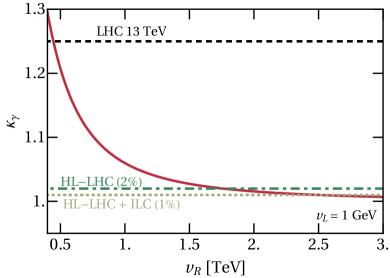
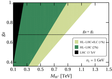
Figure 1: [Left Panel]The solid red curve shows the variation of $\kappa_{\gamma}$, following Eq. (16), with $v_{R}$, for $v_{L}=1$ GeV. The black dashed horizontal line denotes the current $2\sigma$ upper limit on $\kappa_{\gamma}$ at the LHC13 ($\sqrt{s}=13$ TeV, 36 fb^-1 of data) [27, 36]. The dark-green (dash-dotted) and light-green (dotted) horizontal lines denote the projected accuracy of on $\kappa_{\gamma}$ from the HL-LHC (2%) data and HL-LHC+ILC (1%) combined data respectively[37]. Note that the variation in $\kappa_{\gamma}$ with $v_{R}$ and subsequently the limits on $v_{R}$ are independent of $g_{R}$. [Right Panel] The shaded area in black denotes the region in the $g_{R}$-$M_{W^{\prime}}$ plane, excluded at 95% CL from determination of $\kappa_{\gamma}$ at the LHC13. The dark- and light-green shaded regions denote the excluded regions for the projected accuracy of $\kappa_{\gamma}$ determination from the HL-LHC (2%) and HL-LHC+ILC (1%) combined data respectively. While extracting bounds using the projected accuracies at the HL-LHC and HL-LHC+ILC, in both panels, we have assumed the central value of $\kappa_{\gamma}$ to be unity, i.e., consistent with the SM.

In Fig. 1 we display the bounds arising from the current as well as future measurements of $\kappa_{\gamma}$. From the left panel we can see that, irrespective of the value of $g_{R}$, we can rule out $v_{R}$ up to $450$ GeV (implying $M_{W^{\prime}}\gtrsim 170$ GeV for $g_{L}=g_{R}$) at 95% C.L. using the current LHC data[27]. Although this limit is weak compared to the existing bounds on $M_{W^{\prime}}$, it is evident from the left panel of Fig. 1 that, due to the almost horizontal tail of the red curve, once $\kappa_{\gamma}$ is found to be consistent with the SM with accuracy of a few percent at future colliders, a slight improvement in the precision can substantially strengthen the bound on $v_{R}$. To put it into perspective, as shown in Fig. 1, if $\kappa_{\gamma}$ is observed to be in agreement with the SM with a projected accuracy of 2% at the HL-LHC[37, 36], then we can reach $v_{R}\gtrsim 1.7$ TeV, which can complement the bounds from other considerations. Furthermore, if we can attain the accuracy of 1% in the combined measurement of $\kappa_{\gamma}$ at the HL-LHC and ILC[37], then the bound on $v_{R}$ can climb up to $v_{R}\gtrsim 2.5$ TeV. In passing, we note that, although Fig. 1 has been obtained by setting $v_{L}=1$ GeV, we have checked that the plots do not crucially depend on the exact value of $v_{L}$ as long as $v_{L}\lesssim{\cal O}\left(10~{}{\rm GeV}\right)$. Additionally, we have also checked that for $v_{L}\lesssim{\cal O}\left(1~{}{\rm GeV}\right)$, the constraints in Fig. 1 also apply to the more traditional versions of left-right symmetric models where $\chi_{L}$ and $\chi_{R}$ in Eq. (2) are triplets of $SU(2)_{L}$ and $SU(2)_{R}$ respectively.

To summarize, we have pointed out the possibility to put bound on the mass of a $W^{\prime}$-boson arising from an extended gauge structure and the corresponding symmetry breaking scale, using an alternative set of assumptions that does not rely upon the fermionic couplings of the $W^{\prime}$-boson. In view of the fact that the Higgs data is gradually drifting towards the SM expections with increasing accuracy, identifying an SM-like Higgs boson plays an important role in our analysis. The fraction of $M_{W^{\prime}}$, that can be attributed to the EW scale, is then constrained using the $h\to\gamma\gamma$ signal strength measurements. In our example of a left-right symmetric scenario we find that the current data imposes $M_{W^{\prime}}\gtrsim 170$ GeV at 95% C.L. which is at par with the bound from the Michel Parameters[6, 7], but without any assumption about the $W^{\prime}$ coupling to the right-handed leptons. One should also keep in mind that the bounds from direct searches can get considerably diluted for fermiophobic $W^{\prime}$ bosons [38, 39, 40, 41]. Additionally, in the limit of vanishing $W$-$W^{\prime}$ mixing, the production of $W^{\prime}$ via $WZ$ fusion is also suppressed. Thus, considering the fact that the formalism described in this paper does not depend on these factors, our bound using $h\to\gamma\gamma$ signal strength measurements complements the existing limits on $M_{W^{\prime}}$. Moreover, it is also encouraging to note that the bound can rise up to $v_{R}>2.5$ TeV (corresponding to $M_{W^{\prime}}>850$ GeV) if the measurement of the diphoton signal strength is found to be consistent with the SM with a projected accuracy of 1% at the HL-LHC and ILC. Evidently, our current analysis underscores the importance of the precision measurement of the Higgs to diphoton signal strength in current as well as future collider experiments, which can give us potential hints for the scale of NP.

Acknowledgments: D.D., R.P. and J.R. are partially supported by the Swedish Research Council, contract numbers 621-2013-4287 and 2016-05996, as well as by the European Research Council (ERC) under the European Union’s Horizon 2020 research and innovation programme (grant agreement No 668679). R.P. is supported in part by CONICYT grant MEC80170112 as well as by the Ministry of Education, Youth and Sports of the Czech Republic, project LT17018.

Appendix

The Yukawa Lagrangian for the quark sector is given by

$$\mathscr{L}^{q}_{Y}=-\,\overline{Q}_{L}\left(Y_{q}\phi+\widetilde{Y}_{q}\widetilde{\phi}\right)\,Q_{R}\,,$$ (22)

where $Q_{L(R)}=(u_{L(R)},d_{L(R)})^{T}$ denotes the $SU(2)_{L(R)}$ quark doublet and we have suppressed the flavor indices. Therefore, $Y_{q}$ and $\widetilde{Y}_{q}$ are $3\times 3$ Yukawa matrices. From the above Lagrangian, the mass matrices for the up and the down-type quarks can be written as

$$M_{u}=\frac{1}{\sqrt{2}}\left(v_{1}Y_{q}+v_{2}\widetilde{Y}_{q}\right)\,,\qquad M_{d}=\frac{1}{\sqrt{2}}\left(v_{1}\widetilde{Y}_{q}+v_{2}Y_{q}\right)\,.$$ (23)

To diagonalize the mass matrices we make the following unitary transformations on the quark fields:

$$u^{\prime}_{L}=V^{u}_{L}\,u_{L}\,,\qquad d^{\prime}_{L}=V^{d}_{L}\,d_{L}\,,\qquad u^{\prime}_{R}=V^{u}_{R}\,u_{R}\,,\qquad d^{\prime}_{R}=V^{d}_{R}\,d_{R}\,,$$ (24a)

where $q^{\prime}$ represents a physical quark field in the mass basis. Now the bidiagonalization of the mass matrices can be performed as follows:

$${\cal D}_{u}=V_{L}^{u}M_{u}{V_{R}^{u}}^{\dagger}={\rm diag}\{m_{u},m_{c},m_{t}\}\,,\qquad{\cal D}_{d}=V_{L}^{d}M_{d}{V_{R}^{d}}^{\dagger}={\rm diag}\{m_{d},m_{s},m_{b}\}\,.$$ (25)

The Yukawa couplings of $h_{1}$ and $h_{2}$ (defined in Eq. (3)) can be obtained from the Lagrangian of Eq. (22) as follows:

$$\mathscr{L}^{q}_{h_{1},h_{2}}=-\frac{1}{\sqrt{2}}\overline{u}_{L}\left(h_{1}Y_{q}+h_{2}\widetilde{Y}_{q}\right)u_{R}-\frac{1}{\sqrt{2}}\overline{d}_{L}\left(h_{1}\widetilde{Y}_{q}+h_{2}Y_{q}\right)d_{R}\,,$$ (26)

Using the definition of Eq. (11), we can find the projections of $h_{1}$ and $h_{2}$ onto $h$ as follows:

$$\begin{pmatrix}h\\ h^{{}^{\prime}}\\ h^{{}^{\prime\prime}}\\ h^{{}^{\prime\prime\prime}}\end{pmatrix}=\frac{1}{v}\begin{pmatrix}v_{1}&v_{2}&v_{L}&0\\ \cdots&\cdots&\cdots&\cdots\\ \cdots&\cdots&\cdots&\cdots\\ \cdots&\cdots&\cdots&\cdots\end{pmatrix}\begin{pmatrix}h_{1}\\ h_{2}\\ h_{L}\\ h_{R}\end{pmatrix} \Rightarrow \begin{pmatrix}h_{1}\\ h_{2}\\ h_{L}\\ h_{R}\end{pmatrix}=\frac{1}{v}\begin{pmatrix}v_{1}&\cdots&\cdots&\cdots\\ v_{2}&\cdots&\cdots&\cdots\\ v_{L}&\cdots&\cdots&\cdots\\ 0&\cdots&\cdots&\cdots\end{pmatrix}\begin{pmatrix}h\\ h^{{}^{\prime}}\\ h^{{}^{\prime\prime}}\\ h^{{}^{\prime\prime\prime}}\end{pmatrix}\,,$$ (27)

where, in the last step, we have used the fact that the transformation matrix is orthogonal. Now we can use this to replace $h_{1}$ and $h_{2}$ in Eq. (26) and extract the Yukawa couplings of $h$ as

$$\mathscr{L}^{q}_{h} = -\frac{h}{v}\overline{u}^{\prime}_{L}\left[V_{L}^{u}\frac{1}{\sqrt{2}}\left(v_{1}Y_{q}+v_{2}\widetilde{Y}_{q}\right){V_{R}^{u}}^{\dagger}\right]u^{\prime}_{R}-\frac{h}{v}\overline{d}^{\prime}_{L}\left[V_{L}^{d}\frac{1}{\sqrt{2}}\left(v_{2}Y_{q}+v_{1}\widetilde{Y}_{q}\right){V_{R}^{d}}^{\dagger}\right]d^{\prime}_{R}+\mathrm{h.c.}\,,$$ (28)

$$= -\frac{h}{v}\overline{u}^{\prime}_{L}{\cal D}_{u}u^{\prime}_{R}-\frac{h}{v}\overline{d}^{\prime}_{L}{\cal D}_{d}\,d^{\prime}_{R}+\mathrm{h.c.}\,\,\equiv\,\,-\frac{h}{v}\left(\overline{u}^{\prime}{\cal D}_{u}u^{\prime}+\overline{d}^{\prime}{\cal D}_{d}d^{\prime}\right)\,.$$

Evidently, the Yukawa couplings of $h$ are also SM-like.

References

- [1] J. C. Pati and A. Salam, Is Baryon Number Conserved?, Phys. Rev. Lett. 31 (1973) 661–664.
- [2] J. C. Pati and A. Salam, Lepton Number as the Fourth Color, Phys. Rev. D10 (1974) 275–289. [Erratum: Phys. Rev. D11, 703 (1975)].
- [3] R. N. Mohapatra and J. C. Pati, ”Natural” left-right symmetry, Phys. Rev. D11 (1975) 2558–2561.
- [4] G. Senjanovic and R. N. Mohapatra, Exact Left-Right Symmetry and Spontaneous Violation of Parity, Phys. Rev. D12 (1975) 1502–1505.
- [5] Particle Data Group Collaboration, M. Tanabashi et al., Review of particle physics, Phys. Rev. D 98 (Aug, 2018) 030001.
- [6] R. Prieels et al., Measurement of the parameter in polarized muon decay and implications on exotic couplings of the leptonic weak interaction, Phys. Rev. D90 (2014), no. 11 112003, [arXiv:1408.1472].
- [7] OPAL Collaboration, K. Ackerstaff et al., Measurement of the Michel parameters in leptonic tau decays, Eur. Phys. J. C8 (1999) 3–21, [hep-ex/9808016].
- [8] TWIST Collaboration, J. F. Bueno et al., Precise measurement of parity violation in polarized muon decay, Phys. Rev. D84 (2011) 032005, [arXiv:1104.3632].
- [9] M. K. Gaillard and B. W. Lee, Rare Decay Modes of the K-Mesons in Gauge Theories, Phys. Rev. D10 (1974) 897.
- [10] G. Beall, M. Bander, and A. Soni, Constraint on the Mass Scale of a Left-Right Symmetric Electroweak Theory from the - Mass Difference, Phys. Rev. Lett. 48 (1982) 848.
- [11] S. Bertolini, A. Maiezza, and F. Nesti, Present and Future K and B Meson Mixing Constraints on TeV Scale Left-Right Symmetry, Phys. Rev. D89 (2014), no. 9 095028, [arXiv:1403.7112].
- [12] Y. Zhang, H. An, X. Ji, and R. N. Mohapatra, General CP Violation in Minimal Left-Right Symmetric Model and Constraints on the Right-Handed Scale, Nucl. Phys. B802 (2008) 247–279, [arXiv:0712.4218].
- [13] P. Langacker and S. U. Sankar, Bounds on the Mass of W(R) and the W(L)-W(R) Mixing Angle xi in General SU(2)-L x SU(2)-R x U(1) Models, Phys. Rev. D40 (1989) 1569–1585.
- [14] A. Datta and A. Raychaudhuri, Does a Low Mass Right-handed Vector Boson Imply a Departure From Manifest Left-right Symmetry?, Phys. Lett. 122B (1983) 392–396.
- [15] A. Datta and A. Raychaudhuri, Low Mass Right-handed Gauge Bosons, Manifest Left-right Symmetry and the Mass Difference, Phys. Rev. D28 (1983) 1170.
- [16] P. Basak, A. Datta, and A. Raychaudhuri, The Mass Difference in Left-right Symmetric Models and the Right-handed Kobayashi-Maskawa Matrix, Z. Phys. C20 (1983) 305.
- [17] CMS Collaboration, A. M. Sirunyan et al., Search for dijet resonances in proton–proton collisions at = 13 TeV and constraints on dark matter and other models, Phys. Lett. B769 (2017) 520–542, [arXiv:1611.03568]. [Erratum: Phys. Lett.B772,882(2017)].
- [18] ATLAS Collaboration, M. Aaboud et al., Search for new phenomena in dijet events using 37 fb-1 of collision data collected at 13 TeV with the ATLAS detector, Phys. Rev. D96 (2017), no. 5 052004, [arXiv:1703.09127].
- [19] CMS Collaboration, V. Khachatryan et al., Search for W’ decaying to tau lepton and neutrino in proton-proton collisions at 8 TeV, Phys. Lett. B755 (2016) 196–216, [arXiv:1508.04308].
- [20] ATLAS Collaboration, M. Aaboud et al., Search for a new heavy gauge boson resonance decaying into a lepton and missing transverse momentum in 36 fb-1 of collisions at 13 TeV with the ATLAS experiment, Eur. Phys. J. C78 (2018), no. 5 401, [arXiv:1706.04786].
- [21] CMS Collaboration, V. Khachatryan et al., Search for heavy gauge W’ boson in events with an energetic lepton and large missing transverse momentum at 13 TeV, Phys. Lett. B770 (2017) 278–301, [arXiv:1612.09274].
- [22] ATLAS Collaboration, M. Aaboud et al., Search for heavy resonances decaying to a or boson and a Higgs boson in the final state in collisions at TeV with the ATLAS detector, Phys. Lett. B774 (2017) 494–515, [arXiv:1707.06958].
- [23] CMS Collaboration, A. M. Sirunyan et al., Search for heavy resonances that decay into a vector boson and a Higgs boson in hadronic final states at TeV, Eur. Phys. J. C77 (2017), no. 9 636, [arXiv:1707.01303].
- [24] CMS Collaboration, V. Khachatryan et al., Search for heavy neutrinos and bosons with right-handed couplings in proton-proton collisions at , Eur. Phys. J. C74 (2014), no. 11 3149, [arXiv:1407.3683].
- [25] ATLAS Collaboration, G. Aad et al., Search for heavy Majorana neutrinos with the ATLAS detector in pp collisions at TeV, JHEP 07 (2015) 162, [arXiv:1506.06020].
- [26] K. Hsieh, K. Schmitz, J.-H. Yu, and C. P. Yuan, Global Analysis of General SU(2) x SU(2) x U(1) Models with Precision Data, Phys. Rev. D82 (2010) 035011, [arXiv:1003.3482].
- [27] CMS Collaboration, C. Collaboration, Combined measurements of the Higgs boson’s couplings at TeV, .
- [28] T. Blank and W. Hollik, Precision observables in SU(2) x U(1) models with an additional Higgs triplet, Nucl. Phys. B514 (1998) 113–134, [hep-ph/9703392].
- [29] A. G. Akeroyd, M. Aoki, and H. Sugiyama, Probing Majorana Phases and Neutrino Mass Spectrum in the Higgs Triplet Model at the CERN LHC, Phys. Rev. D77 (2008) 075010, [arXiv:0712.4019].
- [30] S. Kanemura and K. Yagyu, Radiative corrections to electroweak parameters in the Higgs triplet model and implication with the recent Higgs boson searches, Phys. Rev. D85 (2012) 115009, [arXiv:1201.6287].
- [31] D. Das and A. Santamaria, Updated scalar sector constraints in the Higgs triplet model, Phys. Rev. D94 (2016), no. 1 015015, [arXiv:1604.08099].
- [32] M. Czakon, J. Gluza, F. Jegerlehner, and M. Zralek, Confronting electroweak precision measurements with new physics models, Eur. Phys. J. C13 (2000) 275–281, [hep-ph/9909242].
- [33] J. Erler, P. Langacker, S. Munir, and E. Rojas, Improved Constraints on Z-prime Bosons from Electroweak Precision Data, JHEP 08 (2009) 017, [arXiv:0906.2435].
- [34] T. Bandyopadhyay, G. Bhattacharyya, D. Das, and A. Raychaudhuri, Reappraisal of constraints on models from unitarity and direct searches at the LHC, Phys. Rev. D98 (2018), no. 3 035027, [arXiv:1803.07989].
- [35] J. F. Gunion, H. E. Haber, G. L. Kane, and S. Dawson, The Higgs Hunter’s Guide, Front. Phys. 80 (2000) 1–404.
- [36] M. Cepeda et al., Higgs Physics at the HL-LHC and HE-LHC, arXiv:1902.00134.
- [37] K. Fujii et al., Physics Case for the International Linear Collider, arXiv:1506.05992.
- [38] A. Donini, F. Feruglio, J. Matias, and F. Zwirner, Phenomenological aspects of a fermiophobic SU(2) x SU(2) x U(1) extension of the standard model, Nucl. Phys. B507 (1997) 51–90, [hep-ph/9705450].
- [39] R. S. Chivukula, B. Coleppa, S. Di Chiara, E. H. Simmons, H.-J. He, M. Kurachi, and M. Tanabashi, A Three Site Higgsless Model, Phys. Rev. D74 (2006) 075011, [hep-ph/0607124].
- [40] H.-J. He, T. M. P. Tait, and C. P. Yuan, New top flavor models with seesaw mechanism, Phys. Rev. D62 (2000) 011702, [hep-ph/9911266].
- [41] H.-C. Cheng and I. Low, TeV symmetry and the little hierarchy problem, JHEP 09 (2003) 051, [hep-ph/0308199].