Searching for cool and cooling X-ray emitting gas in 45 galaxy clusters and groups

Abstract

We present a spectral analysis of cool and cooling gas in 45 cool-core clusters and groups of galaxies obtained from Reflection Grating Spectrometer (RGS) XMM-Newton observations. The high-resolution spectra show Fe XVII emission in many clusters, which implies the existence of cooling flows. The cooling rates are measured between the bulk Intracluster Medium (ICM) temperature and 0.01 keV and are typically weak, operating at less than a few tens of ${\rm M}_{\odot}{\rm\thinspace yr}^{-1}\,$ in clusters, and less than 1 ${\rm M}_{\odot}{\rm\thinspace yr}^{-1}\,$ in groups of galaxies. They are 10-30$\%$ of the classical cooling rates in the absence of heating, which suggests that AGN feedback has a high level of efficiency. If cooling flows terminate at 0.7 keV in clusters, the associated cooling rates are higher, and have a typical value of a few to a few tens of ${\rm M}_{\odot}{\rm\thinspace yr}^{-1}\,$. Since the soft X-ray emitting region, where the temperature $kT<1$ keV, is spatially associated with H$\alpha$ nebulosity, we examine the relation between the cooling rates above 0.7 keV and the H$\alpha$ nebulae. We find that the cooling rates have enough energy to power the total UV-optical luminosities, and are 5 to 50 times higher than the observed star formation rates for low luminosity objects. In 4 high luminosity clusters, the cooling rates above 0.7 keV are not sufficient and an inflow at a higher temperature is required. Further residual cooling below 0.7 keV indicates very low complete cooling rates in most clusters.

1 Introduction

The centre of gravitational systems is one of the key aspects in understanding structure formation. In a hierarchical formation scheme, more massive structures form through merging of smaller components in overdense regions. This self-similar behaviour implies that the dominance of dark matter potential wells in galaxy clusters leads to an inflow of baryons which will deposit the gravitational energy in the core. In hydrostatic equilibrium, such a system will have a high gas temperature and pressure, while preventing overdensity in the central region. However, it is realised that the evolution of galaxy clusters involves processes other than gravitational collapse, such as cooling and feedback (e.g. Kaiser 1991; Wu et al. 2000; Voit et al. 2002). Most evidently, a large fraction of galaxy clusters have been found to host cool cores where the temperature drops towards the centre (e.g. Stewart et al. 1984; Bauer et al. 2005; Cavagnolo et al. 2009; Hudson et al. 2010). The central radiative cooling time drops below a few $10^{8}$ yr (e.g. Fabian et al. 2002), and the entropy $K$ also decreases inwards by a power law (Cavagnolo et al. 2008, 2009; Panagoulia et al. 2014). These suggest that a radiative cooling flow forms in the central region (Fabian 1994), where the energy loss can be observed directly in X-rays by thermal bremsstrahlung. In the cooling flow model, cool gas is compressed by the weight of overlaying gas, and a subsonic inflow of hot gas from outer region is required to sustain pressure. In the absence of heating, cooling rates are predicted to be 100s to more than 1000 $\rm M_{\odot}\,\rm yr^{-1}$ in rich clusters (White et al. 1997; Peres et al. 1998; Allen et al. 2001; Hudson et al. 2010; McDonald et al. 2018). This suggests that we expect not only low temperature components in X-rays but also a large amount of cold molecular gas if it is not consumed in star formation.

On the contrary, observations have shown that the star formation rate is only a small fraction of the predicted cooling rate (Nulsen et al. 1987; Johnstone et al. 1987; O’Dea et al. 2008; Rafferty et al. 2008; McDonald et al. 2018), and the molecular gas detected by CO line emission (Edge 2001; Salomé & Combes 2003) is at least 20 times lower. Meanwhile, far less cooling gas is observed below 1-2 keV in rich clusters (e.g. Kaastra et al. 2001; Peterson et al. 2001; Tamura et al. 2001; David et al. 2001). Peterson et al. 2003 demonstrated that the standard cooling flow model overpredicts the emission lines from the lowest temperatures in X-rays. The analysis of the Centaurus cluster showed that the cooling rate below 0.8 keV is much lower than the cooling rates measured at hotter temperatures (Sanders et al. 2008) ; a similar result was obtained for M87 by Werner et al. (2010). Therefore, cooling must be suppressed by heating mechanisms. AGN feedback is the most likely mechanism, which is energetically strong enough to prevent cooling and yet not overheat the core (for reviews in AGN feedback, see McNamara & Nulsen 2007, 2012 and Fabian 2012). The energy transport mechanism is still uncertain, which should distribute heat spatially within a few tens of kpc. Some possible processes are sound waves and gravity waves (see e.g. Fabian et al. 2005, 2017). Other mechanisms such as dissipation through turbulence and conduction are found to be insufficient to operate the heating process by themselves (Pinto et al. 2015, 2018; Bambic et al. 2018; Voigt & Fabian 2004).

On the other hand, we can still detect mild cooling flows at around 0.4-0.8 keV from the Fe XVII line emission seen in some objects (e.g. Sanders et al. 2008). This suggests that AGN feedback cannot perfectly quench radiative cooling. Further cooling in X-rays is usually not detected from the O VII emission peaking at around 0.1-0.2 keV, though there is evidence of detecting weak O VII emission in less massive clusters and groups of galaxies (Sanders & Fabian 2011; Pinto et al. 2014; Pinto et al. 2016). This raises the question about whether cooling flows can cool further (Fabian et al. 2002). From spatially-resolved Chandra spectra, soft X-ray emitting regions at these temperatures spatially coincide with cooler ultraviolet/optical line-emitting filaments in massive clusters (e.g. Fabian et al. 2001; Fabian et al. 2003; Crawford et al. 2005). These filaments are highly luminous and most of them have luminosities comparable to their soft X-ray emission. This suggests that the cool X-ray emitting gas is likely mixing with cold atomic and molecular line-emitting material. The thermal energy of the hotter X-ray emitting gas is then rapidly radiated at longer wavelengths, e.g., in UV and optical bands (Fabian et al. 2002). To relate properties of optical line-emitting filaments to soft X-ray gas, we convert luminosities into mass cooling rates,

$$\dot{M}=\frac{2}{3}\times\frac{L\mu m_{\rm p}}{kT}$$ (1)

where $\mu$ is the mean particle weight, $m_{\rm p}$ is the proton mass and $k$ is the Boltzmann’s constant. We ignore the $P$d$V$ work done on the cooling gas.

In this paper, we primarily focus on measuring the cooling rates of galaxy clusters, and deduce the efficiency of AGN feedback on suppressing cooling. It is also interesting to compare the measured cooling rates to the energy required to power the observed luminosities at longer wavelengths in filaments. We then search for residual cooling rates below 0.7 keV which determine whether the gas can continue to cool radiatively in X-rays. Finally, the cooling rates are then linked to star formation rates, and we wish to know how they contribute to the massive molecular gas reservoir seen.

Throughout this work, we assume the following cosmological parameters: $H_{0}=73\rm\ km^{-1}Mpc^{-1}$, $\Omega_{\rm M}=0.27$, $\Omega_{\rm\Lambda}=0.73$. The results from literature are corrected using the same cosmology. This paper is organized as follows. Section 2 provides the observations used in our sample and the data reduction procedure. The spectral analysis is presented in section 3, and we discuss the significance of our result in section 4. Finally, we present our conclusions in section 5.

2 Data

In this paper, we present our analysis of the soft X-ray spectra of 45 nearby cool-core galaxy clusters and groups, including the CHEmical Enrichment RGS Sample (CHEERS) sample and the more distant cluster A1835 (Pinto et al. 2015; de Plaa et al. 2017). The CHEERS project includes clusters, groups and elliptical galaxies with the O VIII line detected at 5 $\sigma$ in the Reflection Grating Spectrometer (RGS) spectra (Pinto et al. 2015), and provides a moderately large sample of objects with deep exposure times. Some of the original aims of the CHEERS project were to accurately measure the abundances of key elements, e.g, O and Fe (de Plaa et al. 2017) and constrain the level of turbulence (Pinto et al. 2015). These suggest that the sample is also suitable for measuring the cooling structure of clusters below 1-2 keV, since the relevant O and Fe ionisation stages in the soft X-ray band are strong and usually peak at different temperatures. Furthermore, the CHEERS sample is relatively complete, which contains all suitable targets with different size and bulk temperature within a low redshift of $z\leq 0.1$.

The observations were made by the XMM-Newton satellite, and are listed in Table 1. The satellite has two different types of X-ray instruments: the Reflection Grating Spectrometer and the European Photon Imaging Camera (EPIC). There are two RGS detectors 1 and 2, which are slitless with high spectral solution between 7 and 38 Å  (1.77 to 0.33 keV), and we use the spectra from both detectors for spectral analysis. The MOS 1 and 2 cameras from EPIC are aligned with their associated RGS detectors and have higher spatial resolution, which are used for imaging.

Table 1: XMM-Newton/RGS observations and target properties.

Source a	Observation ID	Total clean time (ks) b	$\it kT_{\rm 1cie}\,^{\it c}$	$\it z(D_{L})\,^{\it d}$	$N_{\rm H,tot}(N_{\rm HI})\,^{\it e}$
2A0335+096	0109870101/0201 0147800201	120.5	1.49$\pm 0.02$	0.0363 (151)	30.7 (17.6)
A85	0723802101/22011	195.8	3.10$\pm 0.12$	0.0551 (236)	3.10 (2.78)
A133	0144310101 0723801301/2001	168.1	2.20$\pm 0.06$	0.0566 (243)	1.67 (1.59)
A262	0109980101/0601 0504780101/0201	172.6	1.32$\pm 0.01$	0.0174 (72.5)	7.15 (5.67)
Perseus 90$\%$ PSF (A426)	0085110101/0201 0305780101	162.8	1.98$\pm 0.03$	0.0179 (74.6)	20.7 (13.6)
Perseus 99$\%$ PSF			1.86$\pm 0.02$
A496	0135120201/0801 0506260301/0401	141.2	2.11$\pm 0.05$	0.0329 (139)	6.12 (3.81)
A1795	0097820101	37.8	3.09$\pm 0.15$	0.0625 (269)	1.24 (1.19)
A1835	0098010101 0147330201 0551830101/0201	294.7	3.89$\pm 0.27$	0.2532 (1230)	2.24 (2.04)
A1991	0145020101	41.6	1.55$\pm 0.05$	0.0587 (252)	2.72 (2.46)
A2029	0111270201 0551780201/0301/0401/0501	155.0	3.45$\pm 0.13$	0.0773 (336)	3.70 (3.25)
A2052	0109920101 0401520301/0501/0601/080	104.3	1.74$\pm 0.04$	0.0355 (150)	3.03 (2.71)
	0401520901/1101/1201/1301/1601/1701
A2199	0008030201/0301/0601 0723801101/1201	129.7	2.57$\pm 0.09$	0.0302 (126)	0.909 (0.888)
A2597	0108460201 0147330101 0723801601/1701	163.9	2.48$\pm 0.14$	0.0852 (373)	2.75 (2.48)
A2626	0083150201 0148310101	56.4	3.07$\pm 0.46$	0.0553 (236)	4.59 (3.82)
A3112	0105660101 0603050101/0201	173.2	2.60$\pm 0.08$	0.0753 (327)	1.38 (1.33)
Centaurus (A3526)	0046340101 0406200101	152.8	1.33$\pm 0.00$	0.0114 (47.2)	12.2 (8.56)
A3581	0205990101 0504780301/0401	123.8	1.33$\pm 0.02$	0.023 (96.2)	5.32 (4.36)
A4038	0204460101 0723800801	82.7	2.31$\pm 0.12$	0.0282 (118)	1.62 (1.53)
A4059	0109950101/0201 0723800901/1001	208.2	2.47$\pm 0.11$	0.0487 (208)	1.26 (1.21)
AS1101	0147800101 0123900101	131.2	1.95$\pm 0.04$	0.0580 (249)	1.17 (1.14)
AWM7	0135950301 0605540101	158.7	1.72$\pm 0.04$	0.0172 (71.8)	11.9 (8.69)
EXO0422-086	0300210401	41.1	2.31$\pm 0.18$	0.0397 (168)	12.4 (7.86)
Fornax (NGC1399)	0012830101 0400620101	123.9	0.98$\pm 0.00$	0.0046 (19.0)	1.56 (1.5)
Hydra A	0109980301 0504260101	110.4	2.44$\pm 0.16$	0.0549 (235)	5.53 (4.68)
Virgo (M87)	0114120101 0200920101	129.0	1.32$\pm 0.00$	0.0043 (16.7)	2.11 (1.94)
MKW3s	0109930101 0723801501	145.6	2.29$\pm 0.08$	0.0442 (188)	3.00 (2.68)
MKW4	0093060101 0723800601/0701	110.3	1.44$\pm 0.02$	0.02 (83.4)	1.88 (1.75)
HCG62	0112270701 0504780501 0504780601	164.6	0.84$\pm 0.01$	0.0147 (61.2)	3.81 (3.31)
NGC5044	0037950101 0584680101	127.1	0.87$\pm 0.00$	0.0093 (38.4)	6.24 (4.87)
NGC5813	0302460101 0554680201/0301/0401	146.8	0.68$\pm 0.00$	0.0065 (26.9)	5.19 (4.37)
NGC5846	0021540101/0501 0723800101/0201	162.8	0.70$\pm 0.00$	0.0057 (23.6)	5.12 (4.29)
M49	0200130101	81.4	0.89$\pm 0.01$	0.0033 (16.0)	1.63 (1.53)
M86	0108260201	63.5	0.79$\pm 0.01$	-0.0008 (16.4)	2.98 (2.67)
M89	0141570101	29.1	0.60$\pm 0.02$	0.0011 (16.5)	2.96 (2.62)
NGC507	0723800301	94.5	1.07$\pm 0.01$	0.0165 (68.5)	6.38 (5.25)
NGC533	0109860101	34.7	0.89$\pm 0.01$	0.0328 (138)	3.38 (3.08)
NGC1316	0302780101 0502070201	165.9	0.68$\pm 0.01$	0.0059 (24.2)	2.56 (2.4)
NGC1404	0304940101	29.2	0.66$\pm 0.01$	0.0065 (26.8)	1.57 (1.51)
NGC1550	0152150101 0723800401/0501	173.4	1.15$\pm 0.01$	0.0129 (51.4)	16.2 (10.2)
NGC3411	0146510301	27.1	0.91$\pm 0.01$	0.0153 (63.5)	4.55 (3.87)
NGC4261	0056340101 0502120101	134.9	0.73$\pm 0.01$	0.0074 (30.5)	1.86 (1.75)
NGC4325	0108860101	21.5	0.89$\pm 0.01$	0.0257 (108)	2.54 (2.32)
NGC4374	0673310101	91.5	0.68$\pm 0.01$	0.0034 (17.0)	3.38 (2.99)
NGC4636	0111190101/0201/0501/0701	102.5	0.67$\pm 0.01$	0.0031 (16.3)	2.07 (1.9)
NGC4649	0021540201 0502160101	129.8	0.84$\pm 0.01$	0.0037 (16.9)	2.23 (2.04)

^(a) The horizontal line between MKW4 and HCG62 differentiates clusters (above) and groups of galaxies (below). For the Perseus clusters, we extracted both the 90 and 99$\%$ PSF spectra. For A1795, we extracted the 97$\%$ PSF spectrum. ^(b) RGS net exposure time. ^(c) The best fit temperatures of the 1 cie model in keV. ^(d) The redshifts are taken from the NED database (https://ned.ipac.caltech.edu/). The luminosity distances in Mpc shown in brackets are either calculated using Wright (2006) (for $z>0.006$) or taken directly from the NED database (for $z<0.006$). ^(e) Total ($N_{\rm H,tot}$) and atomic ($N_{\rm HI}$) hydrogen column densities in $10^{20}\rm\,cm^{-2}$ (see http://www.swift.ac.uk/analysis/nhtot/; Kalberla et al. 2005; Willingale et al. 2013).

2.1 Data reduction

We follow the data reduction procedure used by Pinto et al. (2015) with the XMM-Newton Science Analysis System (SAS) v 13.5.0. The RGS spectra are processed by the SAS task rgsproc, which produces necessary event files, spectra and response matrices. We use emproc for the MOS 1 data, and the SAS task evselect extracts light curves from MOS 1 in the 10-12 keV energy band, allowing us to correct for the contamination from soft-proton flares. The light curves are binned in 100 s intervals and all time bins outside the 2 $\sigma$ level were rejected. We also use template background files based on count rates in CCD 9 to create background spectra, where emission from sources is not expected.

2.2 RGS spectra and MOS 1 images

We use the task rgsproc while setting the xpsfincl mask to include 90$\%$ of the point spread function (PSF) of the first order spectra, which corresponds to a narrow 0.8^′ region containing the central core. The product spectra are subsequently converted into SPEX usable format through the SPEX task trafo. In the conversion process, we stacked different exposures with rgscombine to produce average spectra with high statistics.

RGS spectra are broadened due to spatial (angular) extent of sources in dispersion direction by $\Delta\lambda=0.138\Delta\theta/m$ Å, where $\Delta\lambda$ is the wavelength shift, $\Delta\theta$ is the angular offset from the central source in arcmin and $m$ is the spectral order (see the XMM-Newton Users Handbook for a complete description). We expect that spatial broadening is more important for nearby sources, because angular extents depend on redshifts. To correct for broadening effects, we need to extract surface brightness profile of all sources from their MOS 1 image in the 0.5-1.8 keV energy band with the task vprof, where the products are used as the input of the spatial broadening (lpro) model in SPEX. We perform spectral analysis with SPEX version 3.04.00 with its default proto-Solar abundances of Lodders & Palme (2009). In this work, we use C-statistics (C-stat), and adopt $1\,\sigma$ uncertainties ($\Delta$C-stat = 1) for measurements and $2\,\sigma$ uncertainties ($\Delta$C-stat = 2.71) for upper limits, unless otherwise stated.

3 Spectral analysis

In our analysis, we only include the $7-28$ Å (0.44-1.77 keV) band, since background usually dominates above 28 Å. The spectra are binned by a factor of 5 with the bin size of 0.05 Å, which ensures that a minimum of $\frac{1}{3}$ of RGS spectral resolution is achieved and the data are not overbinned. The typical gas temperature of our low redshift sample is between 0.5 and 4 keV (see Table 1). In the chosen energy band, we expect emission lines from O, Ne, Mg and Fe with different emissivities. For these elements, we set their abundances free relative to hydrogen, except Mg is coupled to Ne to reduce degeneracy in our models which does not significantly change our results. The abundance of N cannot be measured precisely, because the background noise is comparable to the N VII emission at rest frame 24.779 Å. We choose to couple the abundances of N and all the other elements to Fe. These abundances are found to be sub-solar ($Z<Z_{\odot}$) in most objects, though it is possible for the abundance of Fe to be slightly above solar in a few objects such as the Centaurus cluster.

To search for cool and cooling gas, we model the spectra with collisional ionisation equilibrium (cie) and cooling flow (cf) components. The cie component describes an isothermal ICM with a free temperature $T$ and emission measure $EM=n_{\rm e}\,n_{\rm H}\,V$. The X-ray luminosities of cie components are calculated in the 0.01-10 keV band. The cf component measures the cooling rate of an isobaric cooling flow from a maximum temperature $T_{\rm max}$ down to a minimum temperature $T_{\rm min}$ (Mushotzky & Szymkowiak 1988). Such a cooling rate $\dot{M}$ can be derived from a differential emission measure

$$\frac{dEM(T)}{dT}=\frac{5\dot{M}k}{2\mu m_{\rm H}\Lambda(T)}$$ (2)

where $k$ is the Boltzmann constant, $\mu$ is the mean particle weight, $m_{\rm H}$ is the proton mass and $\Lambda(T)$ is the cooling function.

Both the cie and cf components are modified by redshift (red), Galactic absorption (hot) and then convolved by spatial broadening (lpro). In the hot component, we assume a very cold temperature of $T$=0.5 eV with solar abundances (Pinto et al. 2013), and allow hydrogen column density free to vary between $N_{\rm HI}$ and $N_{\rm H,tot}$ (see Table 1; Kalberla et al. 2005; Willingale et al. 2013). The hydrogen column densities are crucial in determining the quality of spectral fits and the magnitude of cooling rates (e.g. 2A0335+096). Although the intrinsic hydrogen column density of the source can usually be ignored, it can potentially be problematic for clusters with powerful AGN (e.g., the Perseus cluster; Churazov et al. 2003), since the emission of the central AGN is processed by the ICM before leaving the clusters. These components assume a Maxwellian electron distribution, and calculate the effect of thermal line broadening. Although turbulence is intrinsic to ICM, it also broadens emission lines usually at a few 100 km/s (e.g. Sanders et al. 2011; Sanders & Fabian 2013; Pinto et al. 2015). For the CHEERS sample, the FWHM of total line widths is at least a few 1000 km/s in the RGS spectra (see Table A.1 in Pinto et al. 2015; Pinto et al. 2016; Bambic et al. 2018). Therefore we ignore turbulent velocity in our sample and fit the scaling parameter $s$ in the lpro component, which can account for any residual broadening. It is possible for our analysis to have minor statistical effects on line widths from stacking multiple observations, though net fluxes are not affected. We include an additional power law (pow) component for clusters with a bright variable AGN (the Perseus and Virgo clusters; see section 3.4). The pow component is not convolved with the spatial profile as the central AGN is a point source. Finally, we assume that any diffuse emission features due to the cosmic X-ray background are smeared out into a broad continuum-like component.

3.1 Isothermal collisional ionisation equilibrium

We start with a single collisional ionisation equilibrium component (1 cie), and the best fit temperatures are shown in Table 1. These temperatures are consistently lower than the cluster values listed by Chen et al. (2007) and Snowden et al. (2008), since the 90$\%$ PSF spectra exclude most of the very hot ($>$4 keV) ICM emission. We demonstrate an example spectral fit of the Centaurus cluster in Fig. 1, where we also show the residuals of both the 1 cie and 2 cie models. It is seen that the Fe XVII/XVIII lines between 14 and 17 Å are underestimated in the 1 cie model, which gives a poor reduced C-stat of 1952/407. The spectral fit is improved significantly the 2 cie model, or by adding an additional cf component (see Sanders et al. 2008 for more detailed analysis on the Centaurus cluster). We attempt to trace any cooler component in our sample first by an additional cie component at a lower temperature (2 cie model; see section 3.2). We then replace this cooler cie component with a cf component cooling from the hotter cie temperature down to 0.01 keV (1 cie + 1 cf model; section 3.3). Finally, we use a two-stage cooling flow model (1 cie + 2 cf model; section 3.3).

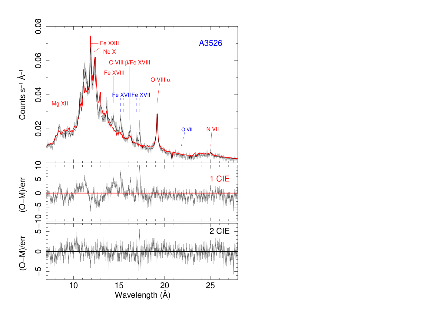
Figure 1: Top: The 90$\%$ PSF RGS spectrum of the Centaurus cluster (grey) with the best-fit isothermal collisional equilibrium model (red) and the 2 temperature model (black). Important emission lines are labelled at the observed wavelengths. Dash lines indicate line emission due to cooling gas below 0.8 keV (Fe XVII) and cooled gas below 0.2 keV (O VII). We show the residuals of both models in the middle (1 cie) and in the bottom (2 cie) panels. Notice that the 2 cie model significantly improves the fit to the Fe XVII, Fe XVIII and Fe XXII emission lines.

3.2 Multi-temperature model

The two temperature (2 cie) model includes the possibility of a cooler gas component. To reduce degeneracy of our model, we assume both cie components have the same abundances, and are convolved by the same lpro component except the Centaurus cluster where the spectral fit is improved by an additional lpro component (Pinto et al. 2016). This is because the Centaurus cluster has a much smaller extent of cooling gas (Sanders et al. 2008; Sanders et al. 2016). The 2 cie model provides sufficient spectral fits for most clusters which is consistent with de Plaa et al. (2017). In Fig. 1, the example of the Centaurus cluster demonstrates that the cooler cie component has a temperature that gives emission from the Fe-L complex and O VII/VIII lines, which dominate the total line emissivity below 1 keV (e.g. see Fig. 2 of Sanders et al. 2010). The emissivity of each ionisation stage peaks at different temperatures, and the best indicators for low temperature gas are O VII lines at around 0.2 keV and Fe XVII lines which have the strongest emissivity below 0.8 keV in the Fe-L complex. However, O VII is usually only found in elliptical galaxies but not massive clusters (except e.g. the Centaurus and Perseus clusters; Sanders & Fabian 2011; Pinto et al. 2016). Since the spatial extent of O VII is generally small (e.g. only in the innermost 5 kpc in the Centaurus cluster; Fabian et al. 2016), it is difficult to measure such lines in our broader 90$\%$ PSF spectra. The temperature of the cooler component cannot be constrained from O VIII emission alone, because it has a much wider temperature range. Hence, we are mainly interested in detecting cooling gas which emits Fe XVII lines peaking at 0.5 keV.

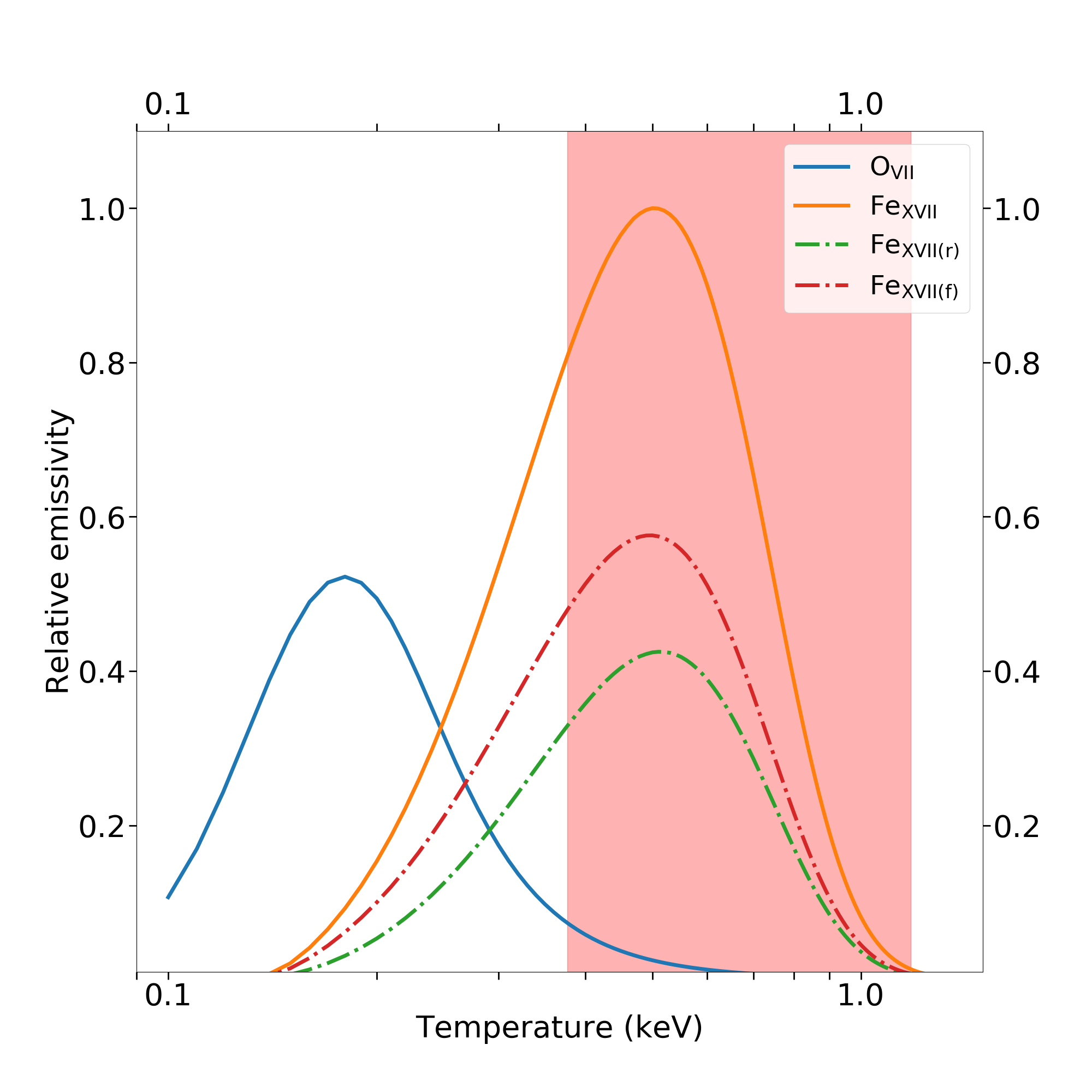
Figure 2: The emissivity of O VII and Fe XVII lines are shown relative to gas temperature. For Fe XVII we include the emissivities of both the resonance and forbidden lines and their sum. The emissivities are normalized such that the peak of the total Fe XVII emissivity is unity. The red shaded region encloses a temperature range 3 times the standard deviation from the average cooler temperature in the 2 cie model. This average temperature excludes four objects with their cooler temperature below 0.4 keV.

We apply the 2 cie model to clusters and two bright groups, and the key parameters are listed in Table 2. There are four objects with a cooler temperature below 0.4 keV, and such a low temperature raises the concern on resonant scattering, which can have a significant impact on measuring the gas temperature through certain emission lines. Since turbulent velocity is generally low in our sample (Pinto et al. 2015), the ICM can be optically thick to radiation at resonant lines. As a result, photons at the resonant wavelengths are absorbed and re-emitted in random directions, and the resonant lines are suppressed in the core and enhanced from the outer region. However, the forbidden line has a much smaller oscillator strength and so is unaffected. Consequently, we expect to see a low Fe XVII resonant-to-forbidden ratio in the 90$\%$ PSF spectra. We also calculate theoretical emissivities of both the Fe XVII and the O VII lines in Fig. 2. The resonant-to-forbidden ratio decreases monotonically below around 1 keV with decreasing temperature, and reaches 0.5 at 0.18 keV where the O VII peaks. In Pinto et al. (2016), it is shown that the Fe XVII resonant-to-forbidden ratio is usually 0.7 or lower. Hence, such a low resonance-to-forbidden ratio can be achieved by either a cool ($<$0.2 keV) component or a cooling ($\sim$0.7 keV) component with resonant scattering or a combination of these situations. Since no O VII lines are observed in most clusters (Pinto et al. 2016), it suggests the cool temperature ($<$0.2 keV) in some objects are likely spurious driven by resonant scattering. It is also possible that background subtraction is affecting the spectra.

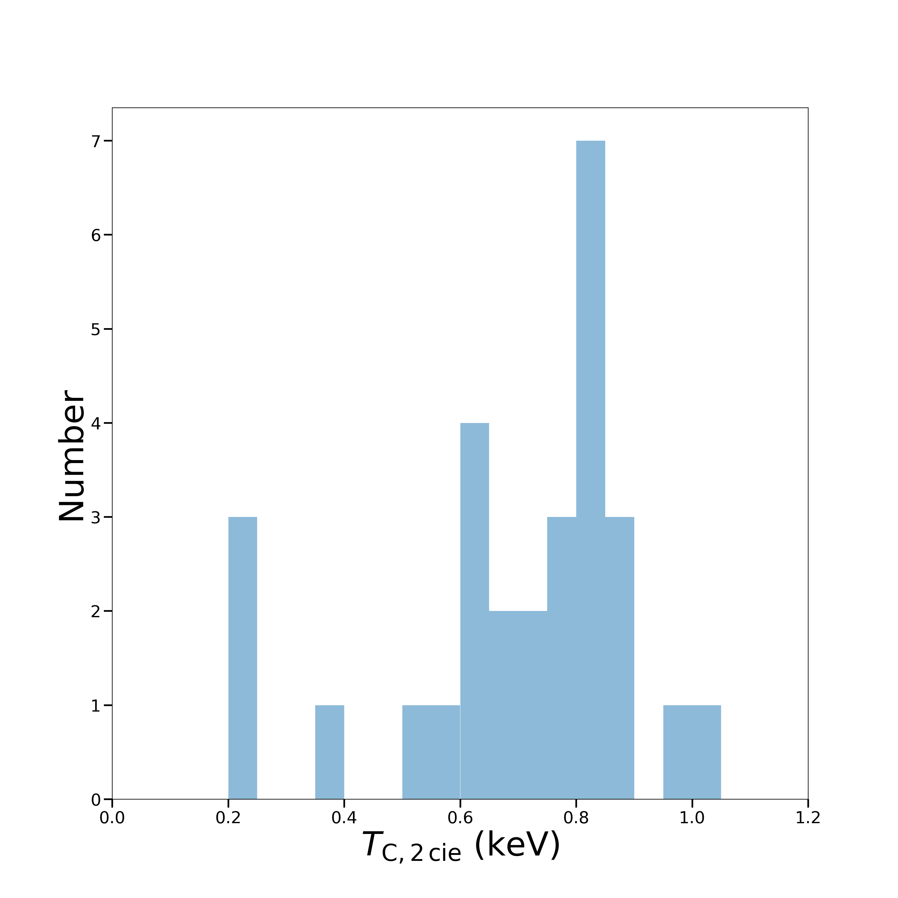
Figure 3: The distribution of the cooler temperature in the 2 cie model in rich clusters with a bin size of 0.05 keV.

Excluding the four objects with a cooler temperature below 0.4 keV, the average temperature of the cooler component is determined to be 0.78$\pm$0.13 keV. We do not expect the intrinsic temperature of the cooler component to distribute much beyond 3 times the standard deviation from the average, or equivalently below a minimum temperature of 0.39 keV. The distribution of the cooler cie temperature is seen in Fig. 3. For EXO0422-086, there is a large uncertainty in the cooler temperature due to limited statistics and the luminosity of the same component only gives an upper limit. Therefore it does not violate our simple expectation of a minimum cooler temperature of 0.39 keV. The best fit models of A1795, AS1101 and MKW3s all give $T_{\rm C,2\,cie}$ at around 0.22 keV. These temperatures are inconsistent with our expectation, and the luminosities also give upper limits. We conclude that these measurements are affected by resonant scattering. For clusters marked by $*$, no H$\alpha$ filament is detect in A2029 (Jaffe et al. 2005), hence we strongly suspect it has no cooler cie component. Both A2626 and Hydra A have limited statistics and the 1 cie model can fit their spectra well (de Plaa et al. 2017). Although there is a large uncertainty in $T_{\rm H,2\,cie}$ in Fornax, the 2 cie model improves the spectral fit significantly.

The X-ray luminosity of the cooler component is usually $10^{42}-10^{43}\,\rm erg\,s^{-1}$. Using equation 2, these luminosities are equivalent to mass flow rates, which are less than 25 ${\rm M}_{\odot}{\rm\thinspace yr}^{-1}\,$ in most objects. This allows us to estimate the volume occupied by the cooler component, the associated gas mass and the cooling time if we know the associated electron density. Cavagnolo et al. (2009) provided spatially resolved analysis of clusters, where they measured the temperatures and electron densities of gas at hot phase. We extrapolate/interpolate these profiles, and evaluate the temperature $T_{\rm e}$ and density $n_{\rm e}$ at a fiducial radius of 5 kpc from the centre. This approximation gives an estimated 5$\%$ uncertainties in both quantities. By assuming the hotter gas is at pressure equilibrium with the cooler cie component, we can estimate the electron density $n_{\rm C}$ associated with the cooler gas by $n_{\rm e}T_{\rm e}=n_{\rm C}T_{\rm C,2\,cie}$. The volume of the component can then be easily evaluated by emission measure in SPEX, which is the product of the electron and hydrogen densities and the volume. If the cool gas is spherical and has an approximately constant density, we can calculate the filling radius $R_{\rm C,2\,cie}$ and the mass of the cooler gas by $M_{\rm C,2\,cie}=1.14\times n_{\rm C}m_{\rm H}V$, where we assume the hydrogen fraction is 75$\%$ and $V$ is the volume. In most objects, we find the filling radius less than 5 kpc and the volume filling ratio of 10-20$\%$. It implies that if the cool gas were distributing throughout the 5 kpc core, the gas has to form either narrow filaments or several separated gas clouds. There are a few objects with the volume filling ratio larger than 100$\%$, which suggests a larger fiducial radius. Since electron densities decrease with larger radii, it is uncertain whether the filling ratio can drop below unity. It is likely that the cooler component in these objects are very extended. On the other hand, we deduce that the mass of the cooler gas is of the order of $10^{8}-10^{9}\,\hbox{${\rm M}_{\odot}{\rm\thinspace yr}^{-1}\,$}$. For A262 and 2A0335+096, we find this mass consistent with the molecular mass within a factor of 2 (Edge 2001; Russell et al. in prep). However, the molecular mass is not consistent with $M_{\rm C,2\,cie}$ for other objects. Finally, we define the cooling time of the cooler cie component to be $t_{\rm cool,2\,cie}=2.31\times 3kT_{\rm C,2\,cie}/2n_{\rm C}\Lambda$, where we get the factor 2.31 by assuming the total hydrogen and ion density is 0.92$n_{\rm C}$, and the proton density is 0.83 $n_{\rm C}$ (McDonald et al. 2018). This is larger but proportional to $M_{\rm C,2\,cie}/\dot{M}_{\rm C,2\,cie}$ using our assumptions.

We do not use the same 2 cie model on most groups of galaxies, where some objects can be well described by an isothermal ICM (e.g. NGC3411). From the improvement of reduced C-stat, we find that a few more groups can be fitted by the 2 cie model, which is mostly consistent with de Plaa et al. (2017). Since these objects typically have 1 cie temperatures less than 1 keV, it is difficult to resolve the temperature of the additional component. Additionally, the cooler cie may suppress the original component and force it to have an unexpectedly high temperature in some objects.

We simulate a spectrum of a cooling flow model from 2 down to 0.01 keV, which is then fitted by a cie component. This cie temperature is found to be 0.86 keV, in agreement with the average temperature of the cooler component. Sanders et al. (2010) performed a Markov Chain Monte Carlo analysis on a simulated cooling flow with three variable temperature components and one component at a fixed temperature. The distribution also showed that there is a component at 0.6-0.8 keV. Sanders et al. (2010) suggested that this particular temperature range is due to gas temperatures which are easily differentiated spectrally. These simulations suggest that the cooler cie component can instead be a cooling flow in clusters. We attempt to trace such a cooling flow with two different models in Section 3.3.

Table 2: Key parameters of the 2 cie model in clusters and two bright groups.

Source	$T_{\rm H,2\,cie}$	$T_{\rm C,2\,cie}$	$L_{\rm C,2\,cie}$	$\dot{M}_{\rm C,2\,cie}$	$R_{\rm C,2\,cie}$	$M_{\rm C,2\,cie}$	$t_{\rm cool,2\,cie}$
2A0335+096	1.71$\pm 0.04$	0.79$\pm 0.03$	650$\pm 60$	54$\pm 5$	5.3$\pm 0.3$	2.8$\pm 0.6$	43$\pm 6$
A85	3.14$\pm 0.12$	0.82$\pm 0.14$	$<$126	$<$10.2	$<$2.15	$<$0.331	$>$26.9
A133	2.37$\pm 0.10$	0.86$\pm 0.06$	160$\pm 40$	12$\pm 3$	4.2$\pm 0.5$	0.8$\pm 0.4$	60$\pm 20$
A262	1.52$\pm 0.03$	0.79$\pm 0.03$	49$\pm 6$	4.1$\pm 0.5$	4.8$\pm 0.4$	0.7$\pm 0.2$	130$\pm 20$
Perseus 90$\%$ PSF	2.25$\pm 0.05$	0.57$\pm 0.03$	190$\pm 10$	22$\pm 2$	2.2$\pm 0.1$	0.50$\pm 0.1$	18$\pm 2$
Perseus 99$\%$ PSF	2.07$\pm 0.03$	0.62$\pm 0.02$	600$\pm 20$	64$\pm 3$	3.3$\pm 0.2$	1.6$\pm 0.3$	20$\pm 2$
A496	2.21$\pm 0.07$	0.83$\pm 0.06$	84$\pm 10$	6.7$\pm 0.8$	2.7$\pm 0.2$	0.40$\pm 0.1$	47$\pm 8$
A1795	3.22$\pm 0.18$	0.18$\pm 0.03$	800$\pm 300$	300$\pm 100$	1.8$\pm 0.4$	0.6$\pm 0.4$	2$\pm 1$
A1835	4.14$\pm 0.18$	0.73$\pm 0.07$	1600$\pm 500$	150$\pm 40$	2.8$\pm 0.4$	1.9$\pm 0.9$	11$\pm 5$
A1991	1.78$\pm 0.11$	0.83$\pm 0.07$	270$\pm 80$	21$\pm 6$	5.8$\pm 0.9$	2.0$\pm 0.9$	80$\pm 30$
A2029 *	3.46$\pm 0.16$	0.64$\pm_{0.63}^{0.86}$	$<$575	$<$59.6	$<$2.19	$<$0.908	$>$12.6
A2052	1.98$\pm 0.07$	0.89$\pm 0.04$	180$\pm 40$	13$\pm 3$	6.0$\pm 0.6$	1.8$\pm 0.6$	110$\pm 30$
A2199	2.66$\pm 0.10$	0.74$\pm 0.06$	60$\pm 10$	5$\pm 1$	2.3$\pm 0.3$	0.25$\pm 0.10$	40$\pm 10$
A2597	2.61$\pm 0.10$	0.83$\pm 0.09$	300$\pm 100$	22$\pm 9$	3.4$\pm 0.7$	1.0$\pm 0.7$	40$\pm 20$
A2626 *	3.28$\pm_{0.43}^{0.58}$	1.02$\pm_{0.33}^{0.48}$	$<$83.8	$<$5.47	$<$8.55	$<$5.16	$>$111
A3112	2.64$\pm 0.09$	0.65$\pm 0.08$	100$\pm 40$	10$\pm 4$	2.0$\pm 0.4$	0.26$\pm 0.16$	20$\pm 10$
Centaurus	1.64$\pm 0.02$	0.82$\pm 0.01$	77$\pm 2$	6.2$\pm 0.2$	3.2$\pm 0.2$	0.38$\pm 0.06$	50$\pm 3$
A3581	1.38$\pm 0.02$	0.62$\pm 0.07$	37$\pm 7$	3.9$\pm 0.7$	3.4$\pm 0.4$	0.4$\pm 0.1$	80$\pm 20$
A4038	2.40$\pm 0.14$	0.54$\pm 0.10$	25$\pm 7$	3.1$\pm 0.8$	2.4$\pm 0.4$	0.2$\pm 0.1$	50$\pm 20$
A4059	2.55$\pm 0.12$	0.84$\pm 0.09$	60$\pm 20$	4$\pm 2$	3.5$\pm 0.7$	0.4$\pm 0.3$	80$\pm 50$
AS1101	1.96$\pm 0.05$	0.23$\pm 0.15$	$<$129	$<$36.6	$<$1.61	$<$0.244	$>$5.51
AWM7	1.98$\pm 0.10$	0.68$\pm 0.04$	28$\pm 4$	2.8$\pm 0.4$	2.7$\pm 0.2$	0.23$\pm 0.06$	70$\pm 10$
EXO0422-086	2.30$\pm 0.16$	0.37$\pm_{0.14}^{0.27}$	$<$59.4	$<$10.6	$<$1.61	$<$0.106	$>$8.25
Fornax	2.70$\pm_{0.63}^{0.77}$	0.95$\pm 0.01$	13$\pm 2$	0.9$\pm 0.1$	/	/	/
Hydra A *	2.44$\pm 0.09$	0.62$\pm_{0.61}^{0.88}$	$<$79.8	$<$8.46	$<$2.09	$<$0.297	$>$29.0
Virgo	1.42$\pm 0.01$	0.80$\pm 0.02$	13$\pm 1$	1.1$\pm 0.1$	2.2$\pm 0.2$	0.11$\pm 0.02$	80$\pm 10$
MKW3s	2.35$\pm 0.09$	0.21$\pm 0.05$	120$\pm 60$	40$\pm 20$	1.7$\pm 0.5$	0.2$\pm 0.2$	5$\pm 4$
MKW4	1.67$\pm 0.16$	1.11$\pm 0.10$	60$\pm 20$	3$\pm 1$	5.2$\pm 0.9$	0.7$\pm 0.4$	170$\pm 90$
HCG62	1.22$\pm 0.10$	0.78$\pm 0.02$	74$\pm 8$	6.3$\pm 0.6$	9.1$\pm 0.6$	2.1$\pm 0.5$	270$\pm 40$
NGC5044	1.27$\pm_{0.16}^{0.29}$	0.86$\pm 0.01$	164$\pm 10$	12.7$\pm 0.8$	10.8$\pm 0.6$	4.2$\pm 0.8$	270$\pm 30$

We define the condition $\frac{x}{\sigma_{x}}>2$ for a value $x$ (except temperature) to be a measurement, otherwise it is considered as an upper limit. This rule does not apply to the last three column due to rounding. The best fit temperatures of the 2 cie model measured in keV. The luminosities of the cooler cie component $L_{\rm C,2\,cie}$ are calculated in the 0.01-10 keV energy band in $10^{40}\,\rm erg\,s^{-1}$, and are converted into mass flow rates $\dot{M}_{\rm C,2\,cie}$ in $\rm M_{\odot}\,\rm yr^{-1}$ using equation 1 (Fabian et al. 2002). Assuming the cool gas at $T_{\rm C,2\,cie}$ is at pressure equilibrium with the hotter gas, it can fill a sphere with effective radius of $R_{\rm C,2\,cie}$ in kpc. Such a sphere with constant density contains the mass of the cool gas $M_{\rm C,2\,cie}$ in $10^{9}\,\hbox{${\rm M}_{\odot}{\rm\thinspace yr}^{-1}\,$}$. The cooling time of the cool gas is also included in $\rm Myr$. Clusters and two bright groups are included in this table, and those marked by $*$ usually have high uncertainties in $T_{\rm H,2\,cie}$ or $T_{\rm C,2\,cie}$ and $L_{\rm C,2\,cie}$ gives upper limits.

3.3 Cooling flow models

3.3.1 One-stage cooling flow model

Table 3: Key parameters of the one-stage and two-stage cooling flow models in clusters and groups.

Source	$\dot{M}_{\rm simple,3Gyr}$	$\dot{M}_{\rm simple,7.7Gyr}$	$\dot{M}_{\rm 1cie+1cf}$	$\dot{M}_{\rm H,\,1cie+2cf}$	$\dot{M}_{\rm C,\,1cie+2cf}$	$L_{\rm H\alpha}$	$\dot{M}_{\rm neb}$	$\dot{M}_{\rm SFR}$	Reference
2A0335+096	112	185	36$\pm 3$	66$\pm 6$	12$\pm 4$	77.6	110	0.4$\pm_{0.1}^{0.2}$	[1]
A85	81.7	142	1.3$\pm 0.7$	$<$4.15	$<$2.82	1.52	2.15	0.1$\pm_{0.1}^{2.5}$	[2]
A133	47.7	62.5	4.3$\pm 0.5$	12$\pm 2$	$<$1.84	1.14	1.61	0.2$\pm_{0.2}^{1.4}$	[2]
A262	3.38	11.4	2.4$\pm 0.2$	5.3$\pm 0.5$	0.9$\pm 0.3$	0.94	1.33	0.21$\pm 0.03$	[3]
Perseus 90$\%$ PSF	306	303	18$\pm 6$	$<$5.33	31$\pm 2$	224	317	70$\pm_{30}^{60}$	[4]
Perseus 99$\%$ PSF	306	303	56$\pm 15$	21$\pm 7$	82$\pm 4$	224	317	70$\pm_{30}^{60}$	[4]
A496	47.6	66.9	3.2$\pm 0.5$	8$\pm 2$	$<$1.92	2.95	4.17	0.18$\pm 0.01$	[2]
A1795	140	224	$<$14.9	$<$19.5	$<$21.9	5.85	8.27	3$\pm_{3}^{13}$	[3]
A1835	1010	1080	80$\pm 30$	$<$114.8	$<$97.3	441	624	110$\pm_{40}^{60}$	[5]
A1991	37.6	45.1	10$\pm 2$	24$\pm 5$	$<$4.80	3.80	5.37	0.7$\pm_{0.5}^{2.8}$	[2]
A2029	204	369	$<$14.8	$<$30.5	$<$24.3	$<$4.8	$<$6.79	0.8$\pm_{0.09}^{0.10}$	[6]
A2052	28.9	53.6	5.7$\pm 0.6$	16$\pm 1$	$<$1.32	1.69	2.39	0.4$\pm_{0.3}^{1.0}$	[2]
A2199	31.8	107	3.2$\pm 0.6$	5$\pm 2$	2$\pm 1$	1.32	1.87	1$\pm_{1}^{9}$	[3]
A2597	279	611	11$\pm 4$	30$\pm 10$	$<$12.3	79.1	112	4$\pm_{2}^{5}$	[6]
A2626	15.4	24.8	0.9$\pm 0.7$	3$\pm 2$	$<$2.18	0.46	0.651	0.2$\pm_{0.2}^{0.7}$	[3]
A3112	75.2	118	6$\pm 2$	$<$8.02	9$\pm 3$	6.75	9.55	0.8$\pm_{0.6}^{1.8}$	[2]
Centaurus	11.7	26.2	3.3$\pm 0.1$	5.5$\pm 0.3$	0.6$\pm 0.1$	1.71	2.42	0.15$\pm_{0.04}^{0.5}$	[7]
A3581	18.8	20.3	3.0$\pm 0.4$	5$\pm 2$	2.1$\pm 0.9$	2.28	3.23	0.6$\pm_{0.4}^{1.7}$	[2]
A4038	16.7	40.1	2.0$\pm 0.5$	$<$2.39	3.1$\pm 0.9$	/	/	/
A4059	10.8	36.5	2.0$\pm 0.5$	4$\pm 2$	$<$1.51	3.90	5.52	0.3$\pm_{0.2}^{1.0}$	[2]
AS1101	156	227	$<$3.80	$<$5.90	$<$5.09	8.23	11.6	0.9$\pm_{0.6}^{1.5}$	[6]
AWM7	3.79	27.7	2.1$\pm 0.3$	2.0$\pm 0.7$	2.2$\pm 0.6$	/	/	0.3$\pm_{0.1}^{0.3}$
EXO0422-086	26.6	38.6	$<$1.53	$<$4.28	$<$2.61	/	/	/
Fornax	/	/	0.04$\pm 0.01$	0.85$\pm 0.05$	$<$0.01	/	/	/
Hydra A	86.4	109	$<$5.25	$<$1.93	$<$10.8	0.272	0.385	4$\pm_{2}^{7}$	[2]
Virgo	11.1	37.4	0.62$\pm 0.03$	2.33$\pm 0.09$	$<$0.07	0.46	0.651	0.1$\pm_{0.1}^{1.8}$	[4]
MKW3s	24.9	48.2	3$\pm 1$	$<$2.10	5$\pm 2$	1.33	1.88	0.3$\pm_{0.2}^{0.4}$	[4]
MKW4	4.55	7.24	0.11$\pm 0.06$	0.9$\pm 0.2$	$<$0.06	/	/	/
HCG62	3.66	4.46	1.5$\pm 0.2$	/	/	0.0827	0.117	0.06$\pm_{0.06}^{1.05}$	[2]
NGC5044	13.5	34.6	$<$0.10	/	/	0.513	0.726	0.20$\pm_{0.05}^{0.06}$	[2]
NGC5813	3.34	4.8	$<$0.08	/	/	0.0414	0.0586	0.04$\pm_{0.01}^{0.01}$	[2]
NGC5846	2.22	4.3	0.43$\pm 0.06$	/	/	0.0722	0.10	0.09$\pm_{0.04}^{0.06}$	[2]

$\dot{M}_{\rm simple,3Gyr}$ and $\dot{M}_{\rm simple,7.7Gyr}$ are the ‘simple’ and classical cooling rates in the absence of heating, which are deduced from Cavagnolo et al. (2009). The measured cooling rates assume isobaric cooling flows (see equation 2), where $\dot{M}_{1cie+1cf}$ is measured from the cie temperature $T_{\rm Max,\,1cie+1cf}$ down to 0.01 keV in the one-stage model (see Table 4), $\dot{M}_{\rm H,\,1cie+2cf}$ is the cooling rate of the hotter cooling flow component from $T_{\rm Max,\,1cie+2cf}$ down to 0.7 keV and $\dot{M}_{\rm C,\,1cie+2cf}$ is measured between 0.7 and 0.01 keV both in the two-stage model. $L_{\rm H\alpha}$ is expressed in $10^{40}\,\rm erg\,\rm s^{-1}$ and converted into $\dot{M}_{\rm neb}$ using equation 3. The references for $L_{\rm H\alpha}$ are [1] Donahue et al. (2007), [2] Hamer et al. (2016), [3] Crawford et al. (1999), [4] Heckman et al. (1989), [5] Wilman et al. (2006), [6] Jaffe et al. (2005), [7] Crawford et al. (2005). We use the star formation rates from McDonald et al. (2018). All of the mass rates are measured in ${\rm M}_{\odot}{\rm\thinspace yr}^{-1}\,$.

Table 4: Key parameters continued.

Source	$T_{\rm Max,\,1cie+1cf}$	$T_{\rm Max,\,1cie+2cf}$	Source	$T_{\rm Max,\,1cie+1cf}$	$T_{\rm Max,\,1cie+2cf}$
2A0335+096	1.66$\pm 0.03$	1.81$\pm 0.05$	Centaurus	1.52$\pm 0.01$	1.82$\pm 0.05$
A85	3.14$\pm 0.13$	3.18$\pm 0.15$	A3581	1.40$\pm 0.02$	1.43$\pm 0.03$
A133	2.36$\pm 0.10$	2.54$\pm 0.14$	A4038	2.46$\pm 0.16$	2.42$\pm 0.15$
A262	1.48$\pm 0.01$	1.60$\pm 0.04$	A4059	2.57$\pm 0.12$	2.64$\pm 0.14$
Perseus 90$\%$ PSF	2.36$\pm 0.06$	2.21$\pm 0.04$	AS1101	1.96$\pm 0.05$	1.96$\pm 0.04$
Perseus 99$\%$ PSF	2.14$\pm 0.02$	2.05$\pm 0.02$	AWM7	2.02$\pm 0.12$	2.02$\pm 0.13$
A496	2.20$\pm 0.05$	2.27$\pm 0.08$	EXO0422-086	2.32$\pm 0.19$	2.30$\pm 0.17$
A1795	3.10$\pm 0.16$	3.12$\pm 0.15$	Fornax	0.99$\pm 0.01$	1.56$\pm 0.04$
A1835	4.34$\pm_{0.32}^{0.22}$	4.36$\pm_{0.33}^{0.25}$	Hydra A	2.44$\pm 0.08$	2.43$\pm 0.09$
A1991	1.71$\pm 0.08$	1.88$\pm 0.14$	Virgo	1.37$\pm 0.01$	1.43$\pm 0.01$
A2029	3.47$\pm 0.14$	3.46$\pm 0.13$	MKW3s	2.34$\pm 0.08$	2.33$\pm 0.08$
A2052	1.87$\pm 0.05$	2.07$\pm 0.07$	MKW4	1.46$\pm 0.01$	1.53$\pm 0.03$
A2199	2.73$\pm 0.11$	2.76$\pm 0.11$	HCG62	0.90$\pm 0.01$	/
A2597	2.62$\pm 0.11$	2.67$\pm 0.11$	NGC5044	0.87$\pm 0.01$	/
A2626	3.22$\pm_{0.37}^{0.54}$	3.38$\pm_{0.47}^{0.62}$	NGC5813	0.68$\pm 0.01$	/
A3112	2.66$\pm 0.09$	2.64$\pm 0.09$	NGC5846	0.75$\pm 0.01$	/

The temperatures of the cie component (the maximum temperature of the cooling flow) in both the one-stage and two-stage models.

Table 5: One-stage model for galaxies.

Source	$\dot{M}_{\rm 1cie+1cf}$	$T_{\rm Max,\,1cie+1cf}$	Source	$\dot{M}_{\rm 1cie+1cf}$	$T_{\rm Max,\,1cie+1cf}$
M49	0.07$\pm 0.02$	0.92$\pm 0.01$	NGC1550	0.5$\pm 0.1$	1.17$\pm 0.01$
M86	0.20$\pm 0.08$	0.84$\pm 0.02$	NGC3411	$<$0.32	0.91$\pm 0.01$
M89	0.3$\pm 2$	0.64$\pm 0.02$	NGC4261	$<$0.10	0.73$\pm 0.01$
NGC507	0.69$\pm 0.06$	1.17$\pm 0.01$	NGC4325	$<$2.67	0.90$\pm 0.02$
NGC533	$<$2.64	0.90$\pm 0.04$	NGC4374	0.2$\pm 0.1$	0.71$\pm 0.04$
NGC1316	0.26$\pm 0.04$	1.34$\pm 0.03$	NGC4636	1.1$\pm 0.2$	0.72$\pm 0.01$
NGC1404	0.6$\pm 0.3$	0.69$\pm 0.03$	NGC4649	$<$0.01	0.84$\pm 0.01$

Only the one-stage cooling flow model is used for galaxies.

The one-stage cooling flow model includes 1 cie and 1 cf components which have the same abundances. We assume that the maximum temperature of the cooling flow is the same as the cie temperature, and the minimum temperature is fixed at 0.01 keV.

We find a low level of cooling rate in most clusters, typically less than $10\,\hbox{${\rm M}_{\odot}{\rm\thinspace yr}^{-1}\,$}$ (see Table 3). For clusters with cie temperature higher than 1.6 keV, the measured cooling rates are compared with the ‘simple’ cooling rates $\dot{M}_{\rm simple}(<r)=M_{\rm gas}(r)/t_{\rm cool}(r)$, where $M_{\rm gas}(r)$ is the total gas mass enclosed within a radius $r$. The radius is determined where the radiative cooling time $t_{\rm cool}(r)$ is 3 Gyr. We use the electron density and the cooling time profiles in Cavagnolo et al. (2009), where we model the electron density by a power law with the function of form $n_{e}=Ar^{b}$. We assume the clusters are spherically symmetric and integrate the electron densities between 0.1 kpc and the radius where the cooling time is 3 Gyr. This calculation will give approximately 20$\%$ systematic uncertainty from the actual density profile and the asymmetry of clusters. As an example, if we use the density profiles of the eastern and western halves of the Centaurus cluster (Sanders et al. 2016), the ‘simple’ cooling rate is slightly lower at $9.5\,\hbox{${\rm M}_{\odot}{\rm\thinspace yr}^{-1}\,$}$, as oppose to $11.7\,\hbox{${\rm M}_{\odot}{\rm\thinspace yr}^{-1}\,$}$ from the symmetric density profile. These ‘simple’ cooling rates are consistent with the clusters values calculated by McDonald et al. 2018. We repeat the same calculation for the classical cooling rates, which have the radiative cooling time of 7.7 Gyr. In this work, we denote the ‘simple’ and classical cooling rates as $\dot{M}_{\rm simple,3Gyr}$ and $\dot{M}_{\rm simple,7.7Gyr}$ respectively . In general, we find that $\dot{M}_{\rm simple,3Gyr}<\dot{M}_{\rm simple,7.7Gyr}$.

Since the ‘simple’ and classical cooling rates can serve as a proxy for predicted cooling rates in the absence of heating, we can infer the efficiency of heating due to feedback between the measured-to-predicted ratio and unity. The distribution is shown in the top panel of Fig. 5 and 6. The great majority of clusters have a measured-to-predicted ratio less than 0.4 if we use $\dot{M}_{\rm simple,3Gyr}$, which is equivalent to a minimum heating efficiency of 60$\%$. 19 out of 22 clusters have a measured-to-predicted ratio less than 0.2. In the $\dot{M}_{\rm simple,7.7Gyr}$ case, the measured cooling rates are less than 30$\%$ of $\dot{M}_{\rm simple,7.7Gyr}$ for all clusters, and less than 10$\%$ in 18 out of 22 clusters, which is consistent with Hudson et al. (2010). We further notice that clusters with upper limits in the measured cooling rates are suppressed more effectively than those with measurements.

For groups, very weak cooling flows are sometimes detected, typically less than $1\,\hbox{${\rm M}_{\odot}{\rm\thinspace yr}^{-1}\,$}$, and many objects only have upper limits in the measured cooling rates (see Table 5). The level of cooling rates is similar to the values reported by Bregman et al. (2005), usually consistent within 1 $\sigma$ uncertainty. The minimum temperature of 0.01 keV is important for groups since their cie temperature is typically less than 1 keV. If we use a higher value, it is likely to overpredict the cooling rates when the range between the maximum and minimum temperatures is very narrow. Note that it is possible that some objects which can be well fitted by the 1 cie model may also be fitted by a single cooling flow model (see e.g. Pinto et al. 2014).

3.3.2 Two-stage cooling flow model

For clusters, it is also possible that the cooling flow terminates at a temperature higher than 0.01 keV, because no O VII is seen in most objects (Pinto et al. 2016). We choose a terminal temperature (i.e. the minimum temperature of the cf component) of 0.7 keV, and use an additional cf component to measure the residual cooling rate between 0.7 and 0.01 keV (two-stage model). This terminal temperature is the average cooler temperature of all objects in the 2 cie model, which is higher than the average terminal temperature of 0.6 keV if we set the terminal temperature free in the one-stage model. For 5 clusters, we show the measured cooling rates with different terminal temperatures $T_{\rm terminal}$ (Fig. 4a), and hence the initial temperatures $T_{\rm initial}$ for the residual cooling rates (Fig. 4b). It is seen that the cooling rates of the hotter cooling flow component gradually decrease with lower terminal temperatures, and do not change our conclusions. The trend is slightly more complicated for the residual cooling rates, where more upper limits are detected. They do not always decrease as the cooling rates of the hotter cooling flow, because fitting the component in a narrower temperature range may boost the measured values. Additionally, we simulate the spectrum of a cooling flow of $100\,\hbox{${\rm M}_{\odot}{\rm\thinspace yr}^{-1}\,$}$ between 0.01 and 5 keV using the response matrix of A133, which is then fitted by two cooling flow components with the terminal temperature of the hotter cooling flow component changing between 0.5 and 0.9 keV, and find that both $\dot{M}_{\rm H,\,1cie+2cf}$ and $\dot{M}_{\rm C,\,1cie+2cf}$ are consistent with $100\,\hbox{${\rm M}_{\odot}{\rm\thinspace yr}^{-1}\,$}$ within 1 $\sigma$ uncertainty. Therefore, we only present our measured cooling rates with a terminal temperature of 0.7 keV in Table 3.

The two-stage cooling flow model has one more free parameter than the one-stage model, which means more degeneracy during spectral fitting. Therefore, we observe more clusters with their cooling rates as upper limits, which has a significant impact on e.g. Perseus and A1835. In general, the cooling rates of hotter cf component are either higher than the residual cooling rates, or consistent within 1 $\sigma$ uncertainty. Both the cooling and residual cooling rates are compared with $\dot{M}_{\rm simple}$ in Fig. 5 and 6. It is seen that the cooling rates above 0.7 keV are suppressed by at least 30$\%$ in most objects if we use $\dot{M}_{\rm simple,3Gyr}$, except A262 which has a measured-to-predicted greater than unity. If we instead use $\dot{M}_{\rm simple,7.7Gyr}$, this ratio becomes 40$\%$. The residual cooling rates are much lower and therefore the ratios seen in the bottom panels are much lower. For approximately 90$\%$ of clusters, the residual cooling rates are suppressed by at least 80$\%$. Therefore, the two-stage cooling flow model suggests that clusters seem to cool only down to 0.7 keV. The cie temperature of both the one-stage and two-stage cooling flow models are listed in Table 4.

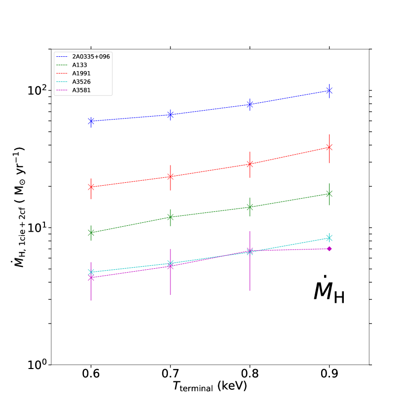
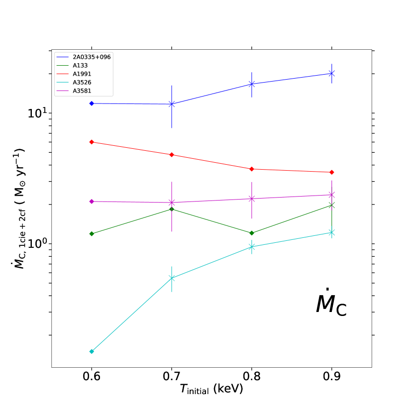
Figure 4: Left: (a) The measured cooling rates between the cie temperature and different terminal temperatures in the two-stage cooling flow model. The diamond shape represents 2 $\sigma$ upper limit. Right: (b) The residual cooling rates between different initial temperatures and 0.01 keV in the two-stage cooling flow model. The initial temperatures match the terminal temperatures of the hotter cooling flow component.

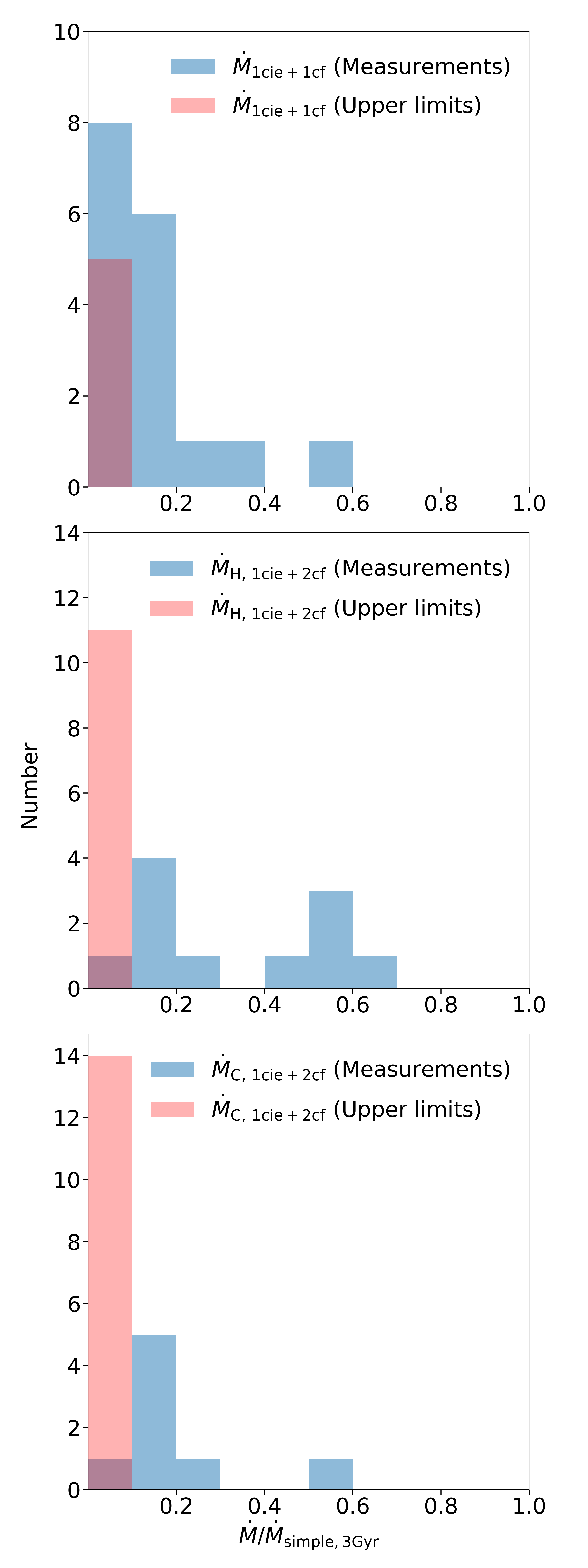
Figure 5: The histograms of the ratio of measured cooling rates to $\dot{M}_{\rm simple,3Gyr}$ for clusters with $T_{\rm Max,\,1cie+2cf}$ $>$ 1.6 keV, where $\dot{M}_{\rm simple,3Gyr}$ are deduced from the gas parameters tabulated by Cavagnolo et al. (2009). Top: cooling rates of the one-stage model. Middle: cooling rates between $T_{\rm Max,\,1cie+2cf}$ and 0.7 keV in the two-stage model. Bottom: the residual cooling rates below 0.7 keV.

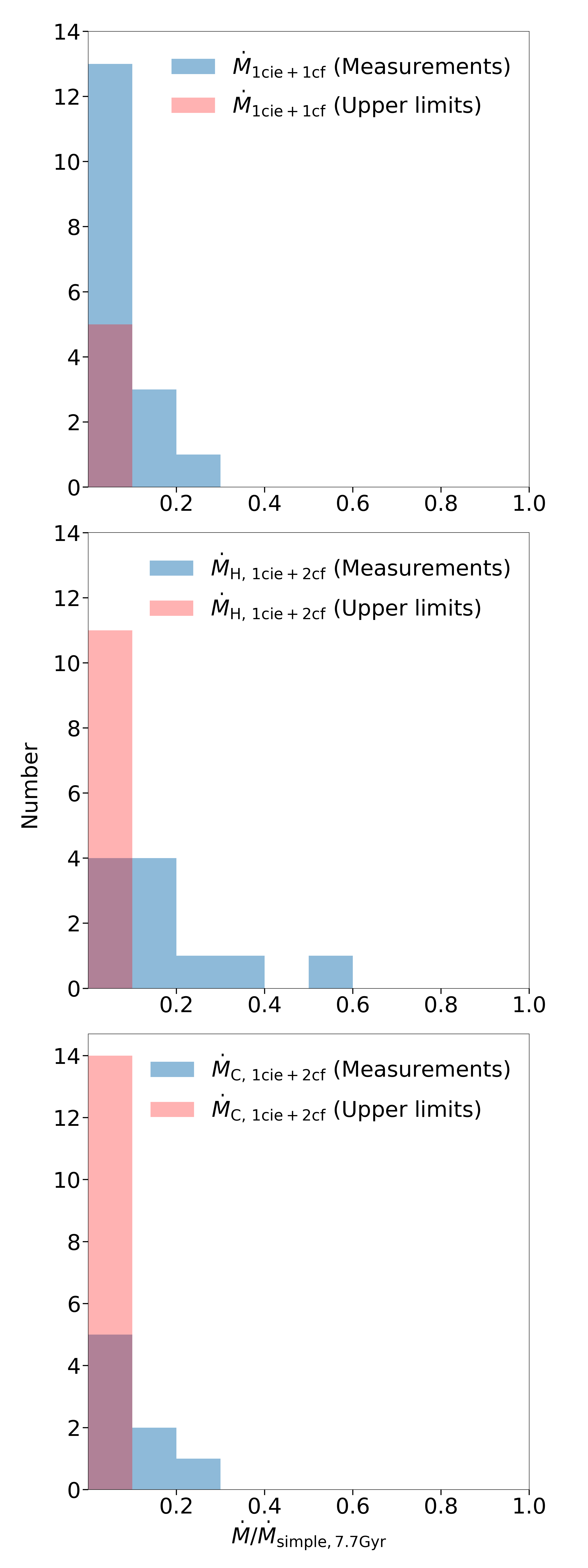
Figure 6: As Fig. 5, but the measured cooling rates are now compared to $\dot{M}_{\rm simple,7.7Gyr}$ (Cavagnolo et al. 2009).

3.3.3 Comparing the cooling flow models

Comparing the two cooling flow models, we find that the cooling rates of the hotter cf component of the two-stage model are generally higher than the one-stage cooling rates. This is because the hotter cf component of the two-stage model need to contribute to Fe XVII emission between a narrow temperature range (0.7-0.9 keV) where its emissivity dominates, and the one-stage model can contribute to Fe XVII emission between 0.01-0.9 keV. Since the two-stage cooling flow model is fitting one more parameter than the one-stage model, we are also interested in whether the two-stage model is statistically better and the difference in spectral fit.

We find that the two-stage model has a lower C-stat than the one-stage model ($\Delta$C-stat$\geq 10$ for 1 degree of freedom) in 9 out of 22 clusters (see Table. 7). However, there are a few special clusters where we prefer the one-stage model, such as Perseus and MKW3s, because the residual cooling rate is higher than the cooling rate above 0.7 keV. For AWM7, we find that there is no difference between the two cooling flow models, both in terms of C-stat and cooling rates. Therefore, we conclude that the one-stage cooling flow is sufficient for AWM7 .

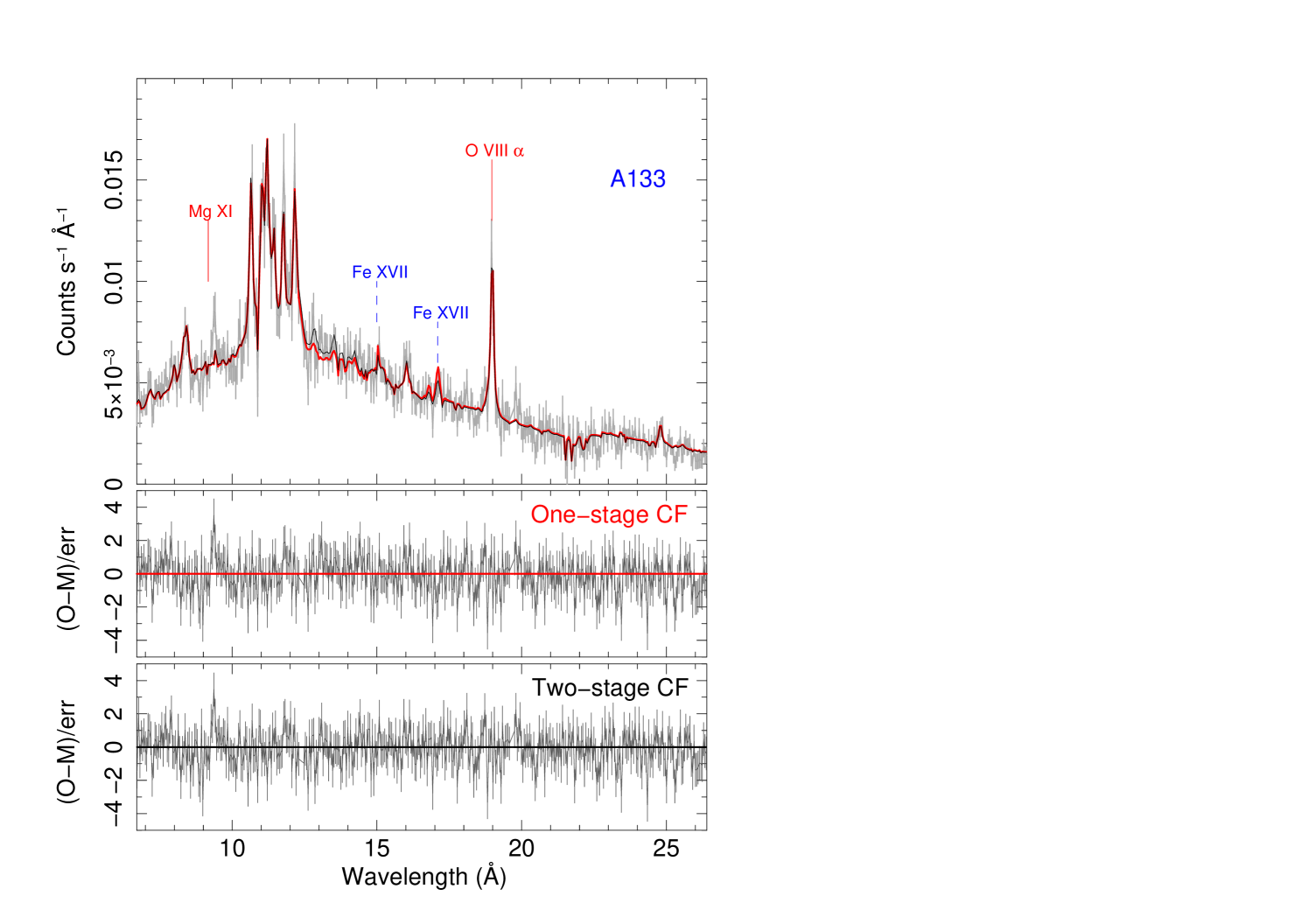
Figure 7: The spectrum (grey) and best fit cooling flow models of A133 in rest wavelength. The spectrum has a peak at around 9.4 Å, which is an artefact and cannot be fitted.

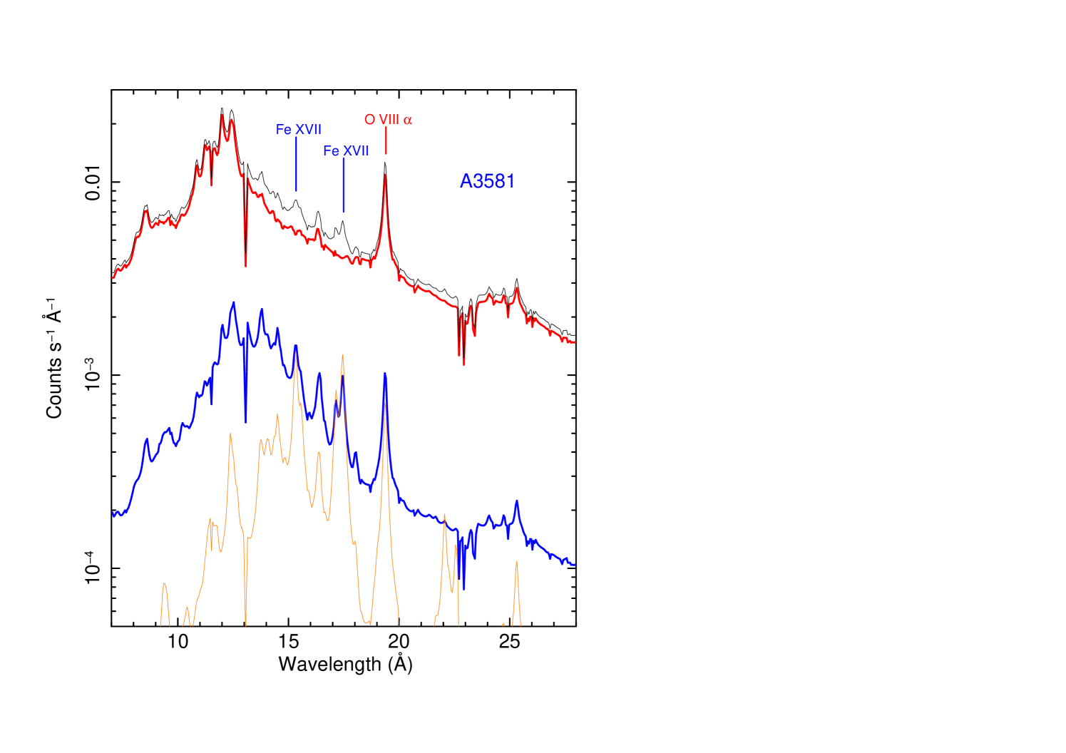
Figure 8: The best fit two-stage cooling flow model of A3581. The top black thin line is the total emission, the thick red line is the contribution from the cie component, the thick blue line is the hotter cooling flow component and the thin orange line at the bottom is the residual cooling flow.

To demonstrate the difference in the spectral fit, we show the spectrum and cooling flow models of A133 in Fig. 7. The two-stage improves the spectral fit to the Fe XVII forbidden line at 17.1 Å, which is related to the cooling gas. Furthermore, the models differ between 12.5 and 14.5 Å, which has emission from different ionisation stages of Fe which peak at hotter temperatures, e.g. Fe XX. However, neither of cooling flow models is significantly better at these wavelengths. We also show the contribution from different components in the two-stage model in Fig. 8. It is seen that the contribution from the two cooling flow components are comparable at important lines, e.g. Fe XVII, O VIII and O VII. In conclusion, we have statistical and spectral evidence that the two-stage cooling flow model is better in at least 9 out of 22 clusters.

3.4 Special clusters

3.4.1 Perseus and Virgo

It is well known that both the X-ray bright Perseus and Virgo clusters have a bright variable AGN at the centre, and it is well described by a pow component. The X-ray emission of the AGN can vary by an order of magnitude in only a few years, and hence we need to fix the parameters of the pow component at the time of our observation. Churazov et al. (2003) found that the AGN emission in Perseus can be well fitted by an absorbed ($N_{\rm H}=10^{21}\,\rm cm^{-2}$) pow component with a photon index of 1.65, where such a column density is comparable to $N_{\rm HI}$ from our own galaxy. The luminosity of the nucleus (OBSID = 0085110101) is constrained to be of the order of $10^{43}\,\rm erg\,\rm s^{-1}$ in the 0.5-8 keV band with 20$\%$ systematic uncertainties. In this work, we choose the emission measure such that the pow component only produces $10^{43}\,\rm erg\,\rm s^{-1}$ in the same energy band. We fit both the 90 and 99$\%$ PSF (0.8^′ and 3.4^′) spectra in this work, and the variable AGN gives an additional 5 and 15 ${\rm M}_{\odot}{\rm\thinspace yr}^{-1}\,$ statistical uncertainty respectively in the one-stage cooling flow model. The actual cooling structure of Perseus is likely to be more complicated than our models because of the existence of the O VII emission (Pinto et al. 2016), which is beyond the scope of this work.

The initial study on Virgo suggests that it is inadequate to use only the stacked spectrum, and hence we perform simultaneous spectral fitting on the non-stacked spectra. The difference in spectra between the two observations is purely due to the variation of the pow component since the ICM emission is constant. We choose the photon index of the first observation to be 2.4 with a flux of $3.76\,\times\,10^{-12}\,\rm erg\,\rm cm^{-2}\,\rm s^{-1}$ in 0.3-8 keV (Observation date: Chandra= 30 July 2000, XMM-Newton= 19 June 2000; see Donato et al. 2004). For the second observation, we use the same photon index and set the emission measure free. The pow component of the second observation yields a flux of $5.19\,\times\,10^{-11}\,\rm erg\,\rm cm^{-2}\,\rm s^{-1}$, which is 13.8 times brighter than the previous observation, and comparable to the ICM luminosity.

3.4.2 Centaurus

In addition to the multi-temperature and cooling flow models, we apply a 5 cf model to both the 90 and 99 $\%$ PSF spectra of the Centaurus cluster, which has been used by Sanders et al. (2008). The temperatures of the cf components are 3.2-2.4, 2.4-1.6, 1.6-0.8, 0.8-0.4, 0.4-0.0808 keV. The components below 0.8 keV are convolved by the same lpro component, and we use a second lpro component for the hotter cf components (3.2 to 0.8 keV) to improve the spectral fit. From the spatial analysis by Sanders et al. (2008), the components below 0.8 keV are located in the innermost core, which supports this critical temperature. The best fit values are shown in Table 6.

We compare these cooling rates of the 90$\%$ PSF spectrum with the two-stage model in section 3.3. The residual cooling rate $\dot{M}_{\rm C,\,1cie+2cf}$ is lower than Comp 4 (0.8-0.4 keV), and Comp 5 only gives an upper limit. They suggest that the cluster cools below 0.7 keV, and stops cooling potentially at around 0.2 keV, where O VII emission was found by Pinto et al. (2016). However, it is difficult to constrain the exact terminal temperature, since the O VII lines are very weak comparing to the continuum.

For the 99$\%$ PSF spectrum, we find our results different from those reported by Sanders et al. (2008). Our model does not fit the hottest cf component (3.2-2.4 keV), which has unexpectedly low upper limits. Further investigation suggests that this can be strongly influenced by different free abundances and the calibration below 8.5 Å  is very poor. Nevertheless, we can still confirm that the Centaurus cluster can be resolved with more than two components (see Table 6 for cf models).

Table 6: The best fit parameters for the Centaurus cluster.

	$\dot{M}$ (90$\%$ PSF)	$\dot{M}$ (99$\%$ PSF)	$\dot{M}$ from Sanders et al. (2008)
Comp 1	$<$ 6.41	$<$ 15.9	46.4$\pm 2.7$
Comp 2	21.2$\pm 2.43$	60.0$\pm 4.56$	32.1$\pm 2.8$
Comp 3	4.69$\pm 0.23$	7.06$\pm 0.30$	6.30$\pm 0.37$
Comp 4	0.99$\pm 0.08$	1.37$\pm 0.13$	2.13$\pm 0.48$
Comp 5	$<$ 0.13	$<$ 0.16	$<$ 2.25

The temperature grids are 3.2-2.4, 2.4-1.6, 1.6-0.8, 0.8-0.4, 0.4-0.0808 keV (from Comp 1 to Comp 5). The cooling rates are in ${\rm M}_{\odot}{\rm\thinspace yr}^{-1}\,$. The second and third columns are our measured values. The fourth column has been revised using the update XSPEC package, where the upper limit in Comp 5 is 1 $\sigma$ only.

Unfortunately, 5-component models cannot be repeated for other objects. Since the thermal structures of clusters are intrinsically different, it is very difficult to define a universal temperature grid. The limited statistics in many objects also forbid us from resolving them further. Hence, we have limited a maximum of 2 cf components for the remaining clusters.

4 Discussion

4.1 The missing soft X-ray emission and H$\alpha$ filaments

Our spectral fits indicate that little cooled gas is seen in the X-ray band below 0.4 keV (Table 2), and the upper limits obtained on $\dot{M}_{\rm C,\,1cie+2cf}$ show little evidence for cooling gas either. Gas may be cooling down due to X-ray emission above $\sim 0.7$ keV but if it does then it does not continue cooling in that way below that energy. Such behaviour is peculiar because the radiative cooling time shortens rapidly as the gas temperature drops.

The situation was modelled by Fabian et al. (2003) in terms of ‘missing’ soft X-ray luminosity, $L_{\rm miss}$. This is the luminosity difference between gas cooling at a rate $\dot{M}$ down to a terminal temperature and gas cooling at the same rate to zero. It was noted that $L_{\rm miss}$ is similar to the luminosity of the optical-UV emission-line nebulosity $L_{\rm neb}$ around the Brightest Cluster Galaxies (BCGs) of the cool core clusters studied, suggesting that $L_{\rm neb}$ was powered by the remaining thermal energy of the cooling gas at $T_{\rm min}$. The hypothesis is supported by the spatial-coincidence of the nebulae and the soft X-ray emission (e.g. Perseus: Fabian et al. 2003; Fabian et al. 2006; Centaurus: Crawford et al. 2005, Fabian et al. 2016; A1795: Fabian et al. 2001, Crawford et al. 2005). In order to capture the full emission from the nebula, we increase the observed H$\alpha$ luminosity by a factor of 15 (Ferland et al. 2009).

The idea agrees with the heating and excitation of the cold gas being due to fast particles (Ferland et al. 2009). Fabian et al. (2011) suggested that the fast particles are the result of interpenetration of the hot and cold gas. In this case, $L_{\rm miss}={3\over 2}\dot{M}_{\rm H,\,1cie+2cf}{{kT}\over{\mu m_{\rm p}}}$ should equal $L_{\rm neb}=15L_{\rm H\alpha}$. We can rewrite the above as $\dot{M}_{\rm H,\,1cie+2cf}=\dot{M}_{\rm neb}$, where

$$\dot{M}_{\rm neb}=0.99\times(\frac{L_{\rm H\alpha}}{10^{40}\,\rm erg\,\rm s^{-1}})(\frac{kT}{1keV})^{-1}\rm M_{\odot}\,\rm yr^{-1},$$ (3)

which is the mass inflow rate into the nebula of particles at energy 0.7 keV. We plot $\dot{M}_{\rm H,\,1cie+2cf}$ against $\dot{M}_{\rm neb}$ in Fig. 9 . Most of the objects lying to the lower left in the plot and $\dot{M}_{\rm H,\,1cie+2cf}>\dot{M}_{\rm neb}$, whereas the opposite is true for the 4 objects up and to the right of the plot.

The situation is more complex than assumed above and we now examine a cluster from the right hand side (Perseus) and the left hand side (Centaurus) in more detail. The Perseus cluster has an extensive H$\alpha$ nebula (Conselice et al. 2001; Fabian et al. 2008), and its H$\alpha$ luminosity is significantly higher than most other objects in our sample. Fabian et al. (2003) used the 4^′ region image of the Perseus cluster and found the filaments are UV/optically bright, where the soft X-ray emission is an energetically minor component. Therefore, we use a broader 3.4^′ spectrum for Perseus (red circle) here to measure the cooling rate. The two-stage cooling model is affected by resonance scattering, and the residual cooling rate below 0.7 keV is stronger than the cooling rate above. This is problematic because we expect residual cooling to be replenished by the cooling flow above 0.7 keV. Instead, we use the cooling rate $55.5\pm\,15.3\rm M_{\odot}\,\rm yr^{-1}$ in the one-stage cooling model, which is 30$\%$ lower than the cooling rate of a one-stage model that cools down to 0.7 keV. To better match this cooling rate to $\dot{M}_{\rm neb}$ we need to use gas at a higher temperature, $\sim T_{\rm Max,\,1cie+1cf}$, rather than 0.7 keV. This would not show up in our analysis here and remains a possible, but unconfirmed solution for powering of the filaments. A detailed study with Chandra of the X-ray spectra of the nebula filaments in the Perseus cluster by Walker et al. (2015) reveals components at both $\sim 2$ keV and 0.7 keV. Several other clusters (M87, Centaurus and A1795) also show the need for the 0.7 keV component. If the Perseus nebula is powered by particles from the surrounding hot gas then an inflow from the surrounding gas at a rate of $\sim 100\hbox{${\rm M}_{\odot}{\rm\thinspace yr}^{-1}\,$}$ is required.

For the Centaurus cluster (the blue point in Fig. 9), to power the nebula requires an inflow of $\sim 2\hbox{${\rm M}_{\odot}{\rm\thinspace yr}^{-1}\,$}$, which is significantly less than our RGS measured value of $\dot{M}_{\rm H,\,1cie+2cf}=5.2\pm 0.2\hbox{${\rm M}_{\odot}{\rm\thinspace yr}^{-1}\,$}$. However, we note that Chandra images of the soft X-ray emission in the cluster reveal emission which is much more extended than the bright filamentary nebula (Sanders et al. 2016). If we refine the estimate of $\dot{M}_{\rm H,\,1cie+2cf}$ to an area coincident with the main filaments using Chandra spectra, then we find that $\dot{M}_{\rm H,\,1cie+2cf}$ drops by a factor of 3 and there is agreement with the particle heating model. Inspection of other clusters with $\dot{M}_{\rm neb}<10\hbox{${\rm M}_{\odot}{\rm\thinspace yr}^{-1}\,$}$ shows that they also have soft emission more extended than the nebula. Note that Hamer et al. (2018) find weak optical [NII] line emission outside the filamentary nebula in the Centaurus cluster that, if common in other clusters, implies that the nebula emission is yet more extended than assumed above.

The nature of the extended 0.7 keV gas component in the Centaurus cluster and other clusters on the left hand side of Fig. 9 is unclear. The low value of $\dot{M}_{\rm H,\,1cie+2cf}$ shows that it is not rapidly radiatively cooling. We compare its luminosity $L_{\rm C,2\,cie}$ (Table 2) with $L_{\rm neb}$ in Fig. 10.

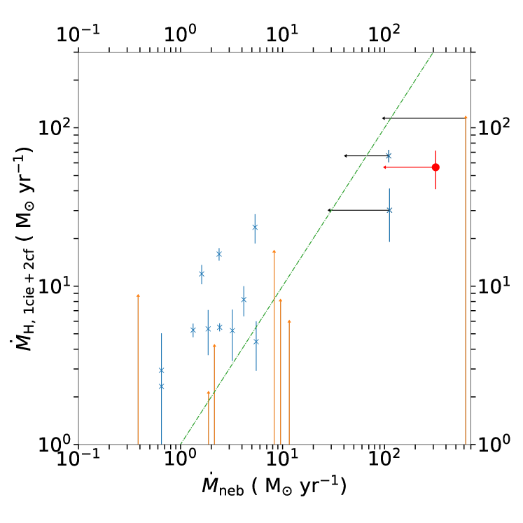
Figure 9: The cooling rates $\dot{M}_{\rm H,\,1cie+2cf}$ in the two-stage model (between $T_{\rm Max,\,1cie+2cf}$ and 0.7 keV) against thermal energy required to sustain emission at longer wavelengths in filaments. The horizontal arrows give the extreme values of $\dot{M}_{\rm neb}$ when using $T_{\rm Max,\,1cie+2cf}$ instead of 0.7 keV in equation 3. For the Perseus cluster, the cooling rate is measured from the 99$\%$ PSF spectrum in the one-stage model (red circle).

For completeness we now also consider the effect of different metallicity, in the light of the inner abundance gradient seen in the Centaurus (Panagoulia et al. 2013; Lakhchaura et al. 2018) and other clusters (Panagoulia et al. 2015). This takes the form of a pronounced drop in Fe and other abundances within the innermost 10 kpc. In Centaurus the Fe abundance is about twice the Solar value at 15–20 kpc and drops to below 0.4 Solar within 5 kpc. Panagoulia et al. (2013) hypothesise that this is due to most metals in stellar mass-loss being in the form of grains which remain trapped in cold clouds. They are then transported out of the cluster centre by the bubbling feedback process and dumped at 10-20 kpc where they mix into the ICM. This means that the region where the ICM temperature is lowest and where a cooling flow might otherwise be expected has a low metallicity. A cooling flow would then produce only weak lines and any detection or limit would rely more on the continuum shape. As examples we have fitted the RGS spectra of the Centaurus cluster and A3581 with the two-stage cooling flow model setting $Z=0.05Z\sun$ for the second stage (cooling from 0.7 to 0.01 keV). The rates for that stage are 15 and $24\,\hbox{${\rm M}_{\odot}{\rm\thinspace yr}^{-1}\,$}$, respectively. We are not claiming that these are solutions for any continuous cooling flow as we have no reason to suspect that the abundance could drop as the temperature passed below 0.7 keV. But the possibility remains that some cooling may occur within the coolest central gas, which may be in the process of being dragged out from the centre (Panagoulia et al. 2013).

It is possible that intrinsic absorption could reduce the level of cooling of the lowest temperature components. The molecular nebula is a potential source of such obscuring gas. We have not included intrinsic absorption in this work and refer the reader to Fig. 18 in Sanders et al. (2008) for the effect it has on the data from the Centaurus cluster. Results for other clusters in our sample will be relatively similar.

In summary, the current spectra neither support nor rule out the idea that the H$\alpha$/CO filaments are powered by interpenetration by the surrounding gas. It remains possible that if it does occur, then it can be from gas at around 0.7 keV in most of the clusters studied but requires hotter gas at $T_{\rm Max,\,1cie+2cf}$ for the most luminous objects.

4.2 Star formation rates

Another aspect we can investigate is whether there is a link between cooling rates and the observed star formation rates. Assuming soft X-ray cooling flows lose their energy to the filaments and the cooled gas is consumed directly in star formation, their difference gives us hints on the rate of change in molecular mass. We compare these parameters in the right panel in Fig. 10. Most clusters and groups have a star formation rate lower than 5 ${\rm M}_{\odot}{\rm\thinspace yr}^{-1}\,$, which is 5 to more than 50 times lower than the measured cooling rate. Only for the more massive clusters Perseus and A1835 with strong star formation activity, the cooling rate close matches the star formation rate and the formation efficiency is around 80 %. This efficiency is higher than the minimum star formation efficiency predicted by McDonald et al. (2018) using the ‘simple’ cooling rates. We find a weak trend of increasing in star formation efficiency with the cooling rate in agreement with McDonald et al. (2018). Since H$\alpha$ filaments are not necessarily aligned with star formation regions (e.g. the Perseus cluster, Canning et al. 2010; Canning et al. 2014), the connection between cooling flows and star formation can be very complicated in massive clusters. The measured cooling rates and upper limits are above the line of unity, and therefore the cooling flows give a net increase in their molecular mass, which accumulates at a level of a few or a few tens of ${\rm M}_{\odot}{\rm\thinspace yr}^{-1}\,$. Assuming the mass of clusters is of the order of $10^{9}-10^{10}\rm M_{\odot}$ (e.g., $4\times 10^{10}\rm M_{\odot}$ in the Perseus cluster, Salomé et al. 2006; $9\times 10^{8}\rm M_{\odot}$ in A262, Edge 2001), a constant mass accumulation rate means that the age of molecular gas is at around a few $10^{8}\rm yr$ to $10^{9}\rm yr$, which is comparable to the age of clusters. Therefore, it is possible that no significant molecular gas content was present at sufficiently early epoch.

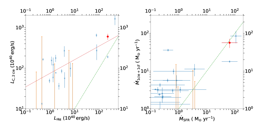
Figure 10: Left: The luminosity of the cooler cie component in the 2 cie model against the H$\alpha$ luminosity. The red dash line represents the best linear fit to the data in the log space. Right: Cooling rates against observed star formation rates (McDonald et al. 2018 references therein). The red circles are the Perseus cluster with 99$\%$ PSF spectrum in both panels.

5 Conclusions

In this paper, we analysed the RGS spectra of the core of 45 clusters and groups of galaxies, and searched for cool and cooling gas. The continuum of the spectra are modelled by a collisional ionisation equilibrium (cie) component, which has a typical bulk temperature of 1-4 keV. Since Fe XVII emission is observed, there is either a cooling flow or a cooler gas component. If cooling flows were taking place in these objects, we can measure the cooling rates with both the one-stage and two-stage cooling flow models. Alternatively, we search for cooler gas with the 2 cie model. The results are as follows.

• In the one-stage cooling flow model, all but one (AWM7) have $\dot{M}/\dot{M}_{\rm simple,3Gyr}$ less than 0.4 and 19 out of 22 clusters have the ratio less than 0.2.

• In the two-stage cooling flow model, we measured the cooling rates between the bulk temperature and 0.7 keV. We find that all clusters but one (A262) have cooling rates less than 70$\%$ of $\dot{M}_{\rm simple,3Gyr}$, and 17 out of 22 clusters have cooling rates less than 30$\%$ of $\dot{M}_{\rm simple,3Gyr}$.

• The residual cooling rates below 0.7 keV are less than 30$\%$ of $\dot{M}_{\rm simple,3Gyr}$ in all clusters except AWM7, and only 10$\%$ in 15/22 clusters. Therefore we find no strong evidence that clusters are rapidly radiatively cooling below 0.7 keV. which suggest that cooling flows appear to stop cooling at around 0.7 keV.

• The 2 cie model gives the cooler temperature between 0.5-0.9 keV in most clusters with the mean temperature of 0.78$\pm$0.13 keV for those higher than 0.4 keV.

• In 9 out of 22 clusters, we have statistical evidence that the two-stage model provides a better spectral fit than the one-stage model ($\Delta$C-stat$\geq 10$ for 1 degree of freedom). For most clusters, we cannot determine whether the 2 cie model or the cooling flow models provide a significantly better spectral fit.

Since the soft X-ray emission happens to be spatially associated with H$\alpha$ nebulosity, we investigated the relation between the cooling rates above 0.7 keV and the total optical-UV luminosities. We find that the detected cooling rates have enough energy to power the total optical-UV luminosities for low luminosity objects, where the soft X-ray region is more extended than the H$\alpha$ nebula. For the 4 high luminosity objects, we observe the opposite situation where the cooling rates are not sufficient. This suggests that if the X-ray cooling gas were powering the nebulae, it requires an inflow at a higher temperature. Finally, we find the cooling rates above 0.7 keV are 5 to 50 times higher than the observed star formation rates, which suggests that it is possible that the mass of the molecular gas reservoir is gradually increasing in most objects.

Appendix A

Table 7: Goodness of fits of different models. In each column, the values are C-statistic/degrees of freedom and their ratio.

Source	1 cie	2 cie	1 cie + 1 cf	1 cie + 2 cf
2A0335+096	627/408 = 1.54	437/406 = 1.08	459/407 = 1.13	436/406 = 1.07
A85	508/406 = 1.25	505/404 = 1.25	507/405 = 1.25	505/404 = 1.25
A133	509/407 = 1.25	453/405 = 1.12	469/406 = 1.16	451/405 = 1.11
A262	653/408 = 1.60	449/406 = 1.11	466/407 = 1.15	440/406 = 1.08
Perseus 90$\%$ PSF	940/408 = 2.30	723/406 = 1.78	758/407 = 1.86	727/406 = 1.79
Perseus 99$\%$ PSF	2246/408 = 5.50	1490/406 = 3.67	1597/407 = 3.92	1554/406 = 3.83
A496	489/409 = 1.20	456/407 = 1.12	468/408 = 1.15	460/407 = 1.13
A1795	432/408 = 1.06	427/406 = 1.05	431/407 = 1.06	430/406 = 1.06
A1835	492/409 = 1.20	480/407 = 1.18	485/408 = 1.19	485/407 = 1.19
A1991	434/406 = 1.07	394/404 = 0.98	400/405 = 0.99	393/404 = 0.97
A2029	427/408 = 1.05	426/406 = 1.05	427/407 = 1.05	427/406 = 1.05
A2052	530/409 = 1.29	442/407 = 1.09	474/408 = 1.16	442/407 = 1.09
A2199	534/407 = 1.31	500/405 = 1.24	505/406 = 1.24	504/405 = 1.24
A2597	502/409 = 1.23	491/407 = 1.21	495/408 = 1.21	492/407 = 1.21
A2626	431/408 = 1.06	429/406 = 1.06	430/407 = 1.06	429/406 = 1.06
A3112	527/408 = 1.29	517/406 = 1.27	520/407 = 1.28	518/406 = 1.28
Centaurus	1952/407 = 4.80	579/403 = 1.44	885/406 = 2.18	694/405 = 1.71
A3581	561/406 = 1.38	502/404 = 1.24	495/405 = 1.22	494/404 = 1.22
A4038	465/407 = 1.14	450/405 = 1.11	453/406 = 1.12	451/405 = 1.11
A4059	462/409 = 1.13	446/407 = 1.10	449/408 = 1.10	446/407 = 1.10
AS1101	461/409 = 1.13	458/407 = 1.13	460/408 = 1.13	459/407 = 1.13
AWM7	542/407 = 1.33	479/405 = 1.18	486/406 = 1.20	486/405 = 1.20
EXO0422-086	474/405 = 1.17	458/403 = 1.14	459/404 = 1.14	458/403 = 1.14
Fornax	747/407 = 1.84	610/405 = 1.51	745/406 = 1.83	665/405 = 1.64
Hydra A	394/409 = 0.96	384/407 = 0.94	384/408 = 0.94	384/407 = 0.94
Virgo	2988/1397= 2.14	2515/1395= 1.80	2633/1396= 1.89	2516/1395= 1.80
MKW3s	501/408 = 1.23	489/406 = 1.21	496/407 = 1.22	492/406 = 1.21
MKW4	442/407 = 1.09	422/405 = 1.04	440/406 = 1.08	430/405 = 1.06
HCG62	594/407 = 1.46	510/405 = 1.26	578/406 = 1.42
NGC5044	696/406 = 1.71	669/404 = 1.66	696/405 = 1.72
M49	630/405 = 1.56		619/404 = 1.53
M86	536/405 = 1.32		532/404 = 1.32
M89	532/406 = 1.31		530/405 = 1.31
NGC507	484/405 = 1.20		440/404 = 1.09
NGC533	522/404 = 1.29		522/403 = 1.30
NGC1316	775/406 = 1.91		709/405 = 1.75
NGC1404	539/406 = 1.33		537/405 = 1.33
NGC1550	541/407 = 1.33		528/406 = 1.30
NGC3411	492/406 = 1.21		492/405 = 1.21
NGC4261	591/406 = 1.46		591/405 = 1.46
NGC4325	422/406 = 1.04		422/405 = 1.04
NGC4374	620/404 = 1.53		616/403 = 1.53
NGC4636	839/409 = 2.05		807/408 = 1.98
NGC4649	671/406 = 1.65		671/405 = 1.66
NGC5813	836/407 = 2.05		836/406 = 2.06
NGC5846	800/407 = 1.97		772/406 = 1.90

Table 8: Relative abundances.

Object	1 cie			2 cie
	O/Fe	Mg/Fe	Fe	O/Fe	Mg/Fe	Fe
2A0335+096	0.92	0.71	0.33	0.75	0.80	0.57
A85	0.57	0.59	0.51	0.56	0.58	0.54
A133	0.57	0.63	0.68	0.54	0.61	0.87
A262	0.72	0.50	0.36	0.66	0.67	0.61
Perseus (90PSF)	1.23	0.50	0.20	0.98	0.64	0.32
Perseus (99PSF)	1.02	0.48	0.21	0.84	0.43	0.32
A496	0.71	0.81	0.49	0.69	0.78	0.57
A1795	1.02	0.99	0.35	0.80	0.98	0.38
A1835	0.85	1.05	0.31	0.78	0.94	0.37
A1991	0.78	0.41	0.49	0.66	0.44	0.76
A2029	1.28	0.46	0.22	1.26	0.45	0.22
A2052	0.71	0.84	0.44	0.64	0.83	0.63
A2199	0.73	0.90	0.43	0.70	0.86	0.50
A2597	0.90	0.80	0.37	0.83	0.77	0.42
A2626	0.51	0.40	0.81	0.50	0.36	0.92
A3112	0.64	0.41	0.52	0.62	0.41	0.56
A3526	0.75	0.24	0.42	0.57	0.54	1.07
A3581	0.86	0.70	0.38	0.80	0.76	0.47
A4038	0.86	0.37	0.41	0.82	0.40	0.50
A4059	0.49	0.68	0.63	0.48	0.66	0.70
AS1101	0.65	0.57	0.40	0.61	0.57	0.41
AWM7	1.08	0.38	0.26	0.83	0.48	0.46
EXO0422-086	0.87	0.85	0.71	0.70	0.73	0.68
Fornax	0.70	1.46	0.51	0.51	0.82	1.22
HYDRA	0.85	0.39	0.30	0.81	0.42	0.30
M87	0.80	0.34	0.42	0.71	0.46	0.58
MKW3s	0.63	0.49	0.40	0.50	0.49	0.44
MKW4	0.57	0.74	1.02	0.53	0.77	1.39
HCG62	0.78	1.94	0.38	0.66	1.32	0.59
NGC5044	0.87	1.20	0.47	0.82	1.03	0.55
M49	0.79	1.32	0.61	/	/	/
M86	1.29	1.62	0.28	/	/	/
M89	1.77	1.64	0.16	/	/	/
NGC507	0.67	1.19	0.66	/	/	/
NGC533	0.80	1.54	0.76	/	/	/
NGC1316	1.79	2.28	0.36	/	/	/
NGC1404	1.07	0.87	0.38	/	/	/
NGC1550	0.73	0.56	0.44	/	/	/
NGC3411	0.54	1.36	1.04	/	/	/
NGC4261	1.11	2.15	0.30	/	/	/
NGC4325	0.61	1.18	0.62	/	/	/
NGC4374	1.56	1.71	0.21	/	/	/
NGC4636	1.11	0.92	0.32	/	/	/
NGC4649	0.94	0.97	0.45	/	/	/
NGC5813	0.94	0.91	0.46	/	/	/
NGC5846	1.23	1.16	0.45	/	/	/

Table 9: Relative abundances continued.

Object	1 cie + 1 cf			1 cie + 2 cf
	O/Fe	Mg/Fe	Fe	O/Fe	Mg/Fe	Fe
2A0335+096	0.74	0.77	0.50	0.71	0.77	0.61
A85	0.56	0.58	0.53	0.56	0.57	0.53
A133	0.53	0.62	0.84	0.54	0.57	0.90
A262	0.61	0.66	0.57	0.63	0.65	0.65
Perseus (90PSF)	0.91	0.55	0.33	0.92	0.62	0.30
Perseus (99PSF)	0.78	0.35	0.33	0.79	0.37	0.30
A496	0.67	0.79	0.56	0.69	0.75	0.57
A1795	0.98	0.95	0.37	0.95	0.96	0.37
A1835	0.73	0.92	0.38	0.74	0.91	0.38
A1991	0.64	0.45	0.68	0.64	0.42	0.79
A2029	1.26	0.45	0.22	1.27	0.45	0.22
A2052	0.64	0.85	0.55	0.64	0.81	0.64
A2199	0.68	0.82	0.51	0.69	0.79	0.50
A2597	0.83	0.78	0.41	0.85	0.75	0.42
A2626	0.50	0.39	0.89	0.50	0.36	0.94
A3112	0.62	0.40	0.55	0.61	0.41	0.55
A3526	0.57	0.39	0.76	0.51	0.49	1.21
A3581	0.70	0.75	0.48	0.69	0.77	0.51
A4038	0.80	0.33	0.50	0.77	0.40	0.50
A4059	0.47	0.67	0.70	0.48	0.64	0.71
AS1101	0.65	0.56	0.40	0.64	0.56	0.40
AWM7	0.79	0.39	0.45	0.81	0.40	0.46
EXO0422-086	0.72	0.73	0.68	0.71	0.73	0.68
Fornax	0.65	1.38	0.53	0.58	1.03	0.87
HYDRA	0.82	0.42	0.30	0.82	0.42	0.30
M87	0.66	0.38	0.54	0.70	0.45	0.58
MKW3s	0.60	0.47	0.43	0.59	0.48	0.44
MKW4	0.56	0.75	1.08	0.55	0.79	1.24
HCG62	0.60	1.56	0.43	/	/	/
NGC5044	0.87	1.20	0.47	/	/	/
M49	0.67	1.14	0.68	/	/	/
M86	1.01	1.29	0.33	/	/	/
M89	1.33	1.65	0.18	/	/	/
NGC507	0.53	0.94	1.08	/	/	/
NGC533	0.78	1.51	0.77	/	/	/
NGC1316	0.87	0.96	0.81	/	/	/
NGC1404	0.86	0.82	0.41	/	/	/
NGC1550	0.72	0.59	0.49	/	/	/
NGC3411	0.54	1.36	1.04	/	/	/
NGC4261	1.11	2.15	0.30	/	/	/
NGC4325	0.60	1.17	0.62	/	/	/
NGC4374	1.27	1.58	0.23	/	/	/
NGC4636	0.78	0.68	0.33	/	/	/
NGC4649	0.94	0.97	0.45	/	/	/
NGC5813	0.94	0.91	0.46	/	/	/
NGC5846	0.90	1.03	0.52	/	/	/

References

- Allen et al. (2001) Allen S. W., Fabian A. C., Johnstone R. M., Arnaud K. A., Nulsen P. E. J., 2001, MNRAS, 322, 589
- Bambic et al. (2018) Bambic C. J., Pinto C., Fabian A. C., Sanders J., Reynolds C. S., 2018, MNRAS, 478, L44
- Bauer et al. (2005) Bauer F. E., Fabian A. C., Sanders J. S., Allen S. W., Johnstone R. M., 2005, MNRAS, 359, 1481
- Bregman et al. (2005) Bregman J. N., Miller E. D., Athey A. E., Irwin J. A., 2005, ApJ, 635, 1031
- Canning et al. (2010) Canning R. E. A., Fabian A. C., Johnstone R. M., Sanders J. S., Conselice C. J., Crawford C. S., Gallagher J. S., Zweibel E., 2010, MNRAS, 405, 115
- Canning et al. (2014) Canning R. E. A., Ryon J. E., Gallagher J. S., Kotulla R., O’Connell R. W., Fabian A. C., Johnstone R. M., Conselice C. J., Hicks A., Rosario D., Wyse R. F. G., 2014, MNRAS, 444, 336
- Cavagnolo et al. (2008) Cavagnolo K. W., Donahue M., Voit G. M., Sun M., 2008, ApJ, 683, L107
- Cavagnolo et al. (2009) Cavagnolo K. W., Donahue M., Voit G. M., Sun M., 2009, ApJS, 182, 12
- Chen et al. (2007) Chen Y., Reiprich T. H., Böhringer H., Ikebe Y., Zhang Y.-Y., 2007, A&A, 466, 805
- Churazov et al. (2003) Churazov E., Forman W., Jones C., Böhringer H., 2003, ApJ, 590, 225
- Conselice et al. (2001) Conselice C. J., Gallagher III J. S., Wyse R. F. G., 2001, AJ, 122, 2281
- Crawford et al. (1999) Crawford C. S., Allen S. W., Ebeling H., Edge A. C., Fabian A. C., 1999, MNRAS, 306, 857
- Crawford et al. (2005) Crawford C. S., Hatch N. A., Fabian A. C., Sanders J. S., 2005, MNRAS, 363, 216
- Crawford et al. (2005) Crawford C. S., Sanders J. S., Fabian A. C., 2005, MNRAS, 361, 17
- David et al. (2001) David L. P., Nulsen P. E. J., McNamara B. R., Forman W., Jones C., Ponman T., Robertson B., Wise M., 2001, ApJ, 557, 546
- de Plaa et al. (2017) de Plaa J., Kaastra J. S., Werner N., Pinto C., Kosec P. e. a., 2017, A&A, 607, A98
- Donahue et al. (2007) Donahue M., Sun M., O’Dea C. P., Voit G. M., Cavagnolo K. W., 2007, AJ, 134, 14
- Donato et al. (2004) Donato D., Sambruna R. M., Gliozzi M., 2004, ApJ, 617, 915
- Edge (2001) Edge A. C., 2001, MNRAS, 328, 762
- Fabian (1994) Fabian A. C., 1994, ARA&A, 32, 277
- Fabian (2012) Fabian A. C., 2012, ARA&A, 50, 455
- Fabian et al. (2002) Fabian A. C., Allen S. W., Crawford C. S., Johnstone R. M., Morris R. G., Sanders J. S., Schmidt R. W., 2002, MNRAS, 332, L50
- Fabian et al. (1985) Fabian A. C., Arnaud K. A., Nulsen P. E. J., Watson M. G., Stewart G. C., McHardy I., Smith A., Cooke B., Elvis M., Mushotzky R. F., 1985, MNRAS, 216, 923
- Fabian et al. (2008) Fabian A. C., Johnstone R. M., Sanders J. S., Conselice C. J., Crawford C. S., Gallagher III J. S., Zweibel E., 2008, Nature, 454, 968
- Fabian et al. (2005) Fabian A. C., Reynolds C. S., Taylor G. B., Dunn R. J. H., 2005, MNRAS, 363, 891
- Fabian et al. (2003) Fabian A. C., Sanders J. S., Crawford C. S., Conselice C. J., Gallagher J. S., Wyse R. F. G., 2003, MNRAS, 344, L48
- Fabian et al. (2001) Fabian A. C., Sanders J. S., Ettori S., Taylor G. B., Allen S. W., Crawford C. S., Iwasawa K., Johnstone R. M., 2001, MNRAS, 321, L33
- Fabian et al. (2006) Fabian A. C., Sanders J. S., Taylor G. B., Allen S. W., Crawford C. S., Johnstone R. M., Iwasawa K., 2006, MNRAS, 366, 417
- Fabian et al. (2011) Fabian A. C., Sanders J. S., Williams R. J. R., Lazarian A., Ferland G. J., Johnstone R. M., 2011, MNRAS, 417, 172
- Fabian et al. (2016) Fabian A. C., Walker S. A., Russell H. R., Pinto C., Canning R. E. A., Salome P., Sanders J. S., Taylor G. B., Zweibel E. G., Conselice C. J., Combes F., Crawford C. S., Ferland G. J., Gallagher III J. S., Hatch N. A., Johnstone R. M., Reynolds C. S., 2016, MNRAS, 461, 922
- Fabian et al. (2017) Fabian A. C., Walker S. A., Russell H. R., Pinto C., Sanders J. S., Reynolds C. S., 2017, MNRAS, 464, L1
- Ferland et al. (2009) Ferland G. J., Fabian A. C., Hatch N. A., Johnstone R. M., Porter R. L., van Hoof P. A. M., Williams R. J. R., 2009, MNRAS, 392, 1475
- Hamer et al. (2016) Hamer S. L., Edge A. C., Swinbank A. M., Wilman R. J., Combes F., Salomé P., Fabian A. C., Crawford C. S., Russell H. R., Hlavacek-Larrondo J., McNamara B. R., Bremer M. N., 2016, MNRAS, 460, 1758
- Hamer et al. (2018) Hamer S. L., Fabian A. C., Russell H. R., Salomé P., Combes F., Olivares V., Polles F. L., Edge A. C., Beckmann R. S., 2018, arXiv e-prints
- Heckman et al. (1989) Heckman T. M., Baum S. A., van Breugel W. J. M., McCarthy P., 1989, ApJ, 338, 48
- Hudson et al. (2010) Hudson D. S., Mittal R., Reiprich T. H., Nulsen P. E. J., Andernach H., Sarazin C. L., 2010, A&A, 513, A37
- Jaffe et al. (2005) Jaffe W., Bremer M. N., Baker K., 2005, MNRAS, 360, 748
- Johnstone et al. (1987) Johnstone R. M., Fabian A. C., Nulsen P. E. J., 1987, MNRAS, 224, 75
- Kaastra et al. (2001) Kaastra J. S., Ferrigno C., Tamura T., Paerels F. B. S., Peterson J. R., Mittaz J. P. D., 2001, A&A, 365, L99
- Kaiser (1991) Kaiser N., 1991, ApJ, 383, 104
- Kalberla et al. (2005) Kalberla P. M. W., Burton W. B., Hartmann D., Arnal E. M., Bajaja E., Morras R., Pöppel W. G. L., 2005, A&A, 440, 775
- Lakhchaura et al. (2018) Lakhchaura K., Werner N., Sun M., Canning R. E. A., Gaspari M., Allen S. W., Connor T., Donahue M., Sarazin C., 2018, MNRAS, 481, 4472
- Lodders & Palme (2009) Lodders K., Palme H., 2009, Meteoritics and Planetary Science Supplement, 72, 5154
- McDonald et al. (2018) McDonald M., Gaspari M., McNamara B. R., Tremblay G. R., 2018, ApJ, 858, 45
- McNamara & Nulsen (2007) McNamara B. R., Nulsen P. E. J., 2007, ARA&A, 45, 117
- McNamara & Nulsen (2012) McNamara B. R., Nulsen P. E. J., 2012, New Journal of Physics, 14, 055023
- Mushotzky & Szymkowiak (1988) Mushotzky R. F., Szymkowiak A. E., 1988, Cooling Flows in Clusters and Galaxies (Nato ASI Series C:). Kluwer Academic Publishers
- Nulsen et al. (1987) Nulsen P. E. J., Johnstone R. M., Fabian A. C., 1987, Proceedings of the Astronomical Society of Australia, 7, 132
- O’Dea et al. (2008) O’Dea C. P., Baum S. A., Privon G., Noel-Storr J., Quillen A. C., Zufelt N., Park J., Edge A., Russell H., Fabian A. C., Donahue M., Sarazin C. L., McNamara B., Bregman J. N., Egami E., 2008, ApJ, 681, 1035
- Panagoulia et al. (2013) Panagoulia E. K., Fabian A. C., Sanders J. S., 2013, MNRAS, 433, 3290
- Panagoulia et al. (2014) Panagoulia E. K., Fabian A. C., Sanders J. S., 2014, MNRAS, 438, 2341
- Panagoulia et al. (2015) Panagoulia E. K., Sanders J. S., Fabian A. C., 2015, MNRAS, 447, 417
- Peres et al. (1998) Peres C. B., Fabian A. C., Edge A. C., Allen S. W., Johnstone R. M., White D. A., 1998, MNRAS, 298, 416
- Peterson et al. (2003) Peterson J. R., Kahn S. M., Paerels F. B. S., Kaastra J. S., Tamura T., Bleeker J. A. M., Ferrigno C., Jernigan J. G., 2003, ApJ, 590, 207
- Peterson et al. (2001) Peterson J. R., Paerels F. B. S., Kaastra J. S., Arnaud M., Reiprich T. H., Fabian A. C., Mushotzky R. F., Jernigan J. G., Sakelliou I., 2001, A&A, 365, L104
- Pinto et al. (2018) Pinto C., Bambic C. J., Sanders J. S., Fabian A. C., McDonald M., Russell H. R., Liu H., Reynolds C. S., 2018, MNRAS, 480, 4113
- Pinto et al. (2016) Pinto C., Fabian A. C., Ogorzalek A., Zhuravleva I., Werner N., Sanders J., Zhang Y.-Y., Gu L., de Plaa J., Ahoranta J., Finoguenov A., Johnstone R., Canning R. E. A., 2016, MNRAS, 461, 2077
- Pinto et al. (2014) Pinto C., Fabian A. C., Werner N., Kosec P., Ahoranta J., de Plaa J., Kaastra J. S., Sanders J. S., Zhang Y.-Y., Finoguenov A., 2014, A&A, 572, L8
- Pinto et al. (2013) Pinto C., Kaastra J. S., Costantini E., de Vries C., 2013, A&A, 551, A25
- Pinto et al. (2015) Pinto C., Sanders J. S., Werner N., de Plaa J., Fabian A. C., Zhang Y.-Y., Kaastra J. S., Finoguenov A., Ahoranta J., 2015, A&A, 575, A38
- Rafferty et al. (2008) Rafferty D. A., McNamara B. R., Nulsen P. E. J., 2008, ApJ, 687, 899
- Salomé & Combes (2003) Salomé P., Combes F., 2003, A&A, 412, 657
- Salomé et al. (2006) Salomé P., Combes F., Edge A. C., Crawford C., Erlund M., Fabian A. C., Hatch N. A., Johnstone R. M., Sanders J. S., Wilman R. J., 2006, A&A, 454, 437
- Sanders & Fabian (2011) Sanders J. S., Fabian A. C., 2011, MNRAS, 412, L35
- Sanders & Fabian (2012) Sanders J. S., Fabian A. C., 2012, MNRAS, 421, 726
- Sanders & Fabian (2013) Sanders J. S., Fabian A. C., 2013, MNRAS, 429, 2727
- Sanders et al. (2008) Sanders J. S., Fabian A. C., Allen S. W., Morris R. G., Graham J., Johnstone R. M., 2008, MNRAS, 385, 1186
- Sanders et al. (2010) Sanders J. S., Fabian A. C., Frank K. A., Peterson J. R., Russell H. R., 2010, MNRAS, 402, 127
- Sanders et al. (2011) Sanders J. S., Fabian A. C., Smith R. K., 2011, MNRAS, 410, 1797
- Sanders et al. (2010) Sanders J. S., Fabian A. C., Smith R. K., Peterson J. R., 2010, MNRAS, 402, L11
- Sanders et al. (2016) Sanders J. S., Fabian A. C., Taylor G. B., Russell H. R., Blundell K. M., Canning R. E. A., Hlavacek-Larrondo J., Walker S. A., Grimes C. K., 2016, MNRAS, 457, 82
- Snowden et al. (2008) Snowden S. L., Mushotzky R. F., Kuntz K. D., Davis D. S., 2008, A&A, 478, 615
- Stewart et al. (1984) Stewart G. C., Fabian A. C., Jones C., Forman W., 1984, ApJ, 285, 1
- Tamura et al. (2001) Tamura T., Kaastra J. S., Peterson J. R., Paerels F. B. S., Mittaz J. P. D., Trudolyubov S. P., Stewart G., Fabian A. C., Mushotzky R. F., Lumb D. H., Ikebe Y., 2001, A&A, 365, L87
- Voigt & Fabian (2004) Voigt L. M., Fabian A. C., 2004, MNRAS, 347, 1130
- Voit et al. (2002) Voit G. M., Bryan G. L., Balogh M. L., Bower R. G., 2002, ApJ, 576, 601
- Walker et al. (2015) Walker S. A., Kosec P., Fabian A. C., Sanders J. S., 2015, MNRAS, 453, 2480
- Werner et al. (2010) Werner N., Simionescu A., Million E. T., Allen S. W., Nulsen P. E. J., von der Linden A., Hansen S. M., Böhringer H., Churazov E., Fabian A. C., Forman W. R., Jones C., Sanders J. S., Taylor G. B., 2010, MNRAS, 407, 2063
- White et al. (1997) White D. A., Jones C., Forman W., 1997, MNRAS, 292, 419
- Willingale et al. (2013) Willingale R., Starling R. L. C., Beardmore A. P., Tanvir N. R., O’Brien P. T., 2013, MNRAS, 431, 394
- Wilman et al. (2006) Wilman R. J., Edge A. C., Swinbank A. M., 2006, MNRAS, 371, 93
- Wright (2006) Wright E. L., 2006, PASP, 118, 1711
- Wu et al. (2000) Wu K. K. S., Fabian A. C., Nulsen P. E. J., 2000, MNRAS, 318, 889