Initial phases of high-mass star formation: A multiwavelength study towards the extended green object G12.42+0.50

Abstract

We present a multiwavelength study of the extended green object, G12.42+0.50 in this paper. The associated ionized, dust, and molecular components of this source are studied in detail employing various observations at near-, mid- and far-infrared, submillimeter and radio wavelengths. Radio continuum emission mapped at 610 and 1390 MHz, using the Giant Meterwave Radio Telescope, India, advocates for a scenario of coexistence of an UC H ii region and an ionized thermal jet possibly powered by the massive young stellar object, IRAS 18079-1756 with an estimated spectral type of $\rm B1-B0.5$. Shock-excited lines of H₂ and [FeII], as seen in the near-infrared spectra obtained with UKIRT-UIST, lend support to this picture. Cold dust emission shows a massive clump of mass 1375 M_⊙ enveloping G12.42+0.50. Study of the molecular gas kinematics using the MALT90 and JCMT archival data unravels the presence of both infall activity and large-scale outflow suggesting an early stage of massive star formation in G12.42+0.50. A network of filamentary features are also revealed merging with the massive clump mimicking a hub-filament layout. Velocity structure along these indicate bulk inflow motion.

1 INTRODUCTION

Massive stars ($\rm M\gtrsim 8M_{\odot}$) play a vital role in the evolution of the universe given their radiative, mechanical and chemical feedback. They dictate the energy budget of the galaxies through powerful radiation, strong winds and supernovae events. Despite this, most aspects of the processes involved in their formation are far less understood in contrast to the low-mass regime. A universal theory elucidating the formation mechanism across the mass range, though much sought after, is still not well established. Tremendous efforts have been going on, since the last decade or so, to investigate whether high-mass star formation can be understood as a ‘scaled-up’ version of the processes involved in the low-mas domain via the Core Accretion hypothesis. This advocates for formation of high-mass stars from pre-stellar cores to form single or binary protostars with enhanced accretion via a rotationally supported disk that also launches protostellar outflows. This model adequately circumvents the ‘radiation pressure problem’, while leaving many questions open regarding the timescales of collapse and fragmentation in massive cores. Alternate theories, like Competitive Accretion and Protostellar Merger, have also been proposed as viable mechanisms. The debate is still not sealed on the preferred mechanism and the influence of prevailing conditions on each. On the observational front, probing the early stages of massive star formation, in particular, remains a challenge. Rarity of sources (owing to fast evolutionary time scales), large distances, complex, embedded and influenced environment and high extinction are factors which hinder the building up of a proper observational database crucial for validating proposed theories. The current status on the theoretical and observational scenarios of high-mass star formation can be found in the excellent reviews by Tan et al. (2014) and Motte et al. (2018) which also give an update on the literature in this field.

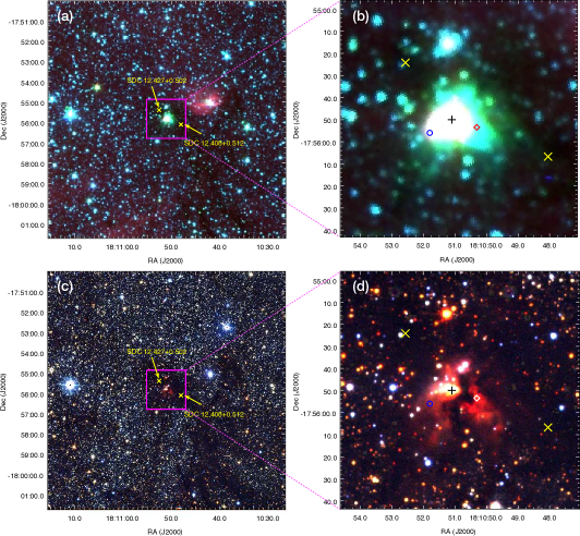
Figure 1: (a) Colour composite image of the region around G12.42+0.50 using IRAC 3.6 $\rm\mu m$ (blue), 4.5 $\rm\mu m$ (green) and 8.0 $\rm\mu m$ (red) bands. (b) A zoom-in showing the EGO G12.42+0.50. IRDCs are shown with the ‘$\times$’ symbol and the position of IRAS 18079-1756 associated with G12.42+0.50 is indicated with a diamond mark. The cross marks the position of the 2MASS point source, J18105109-1755496. The location of the $\rm H_{2}O$ maser is shown as a blue circle. (c) and (d) are colour composites created from the UKIDSS $J$ (1.25 $\rm\mu m$), $H$ (1.63 $\rm\mu m$) and $K$ (2.20 $\rm\mu m$) band data, covering the same area as in (a) and (b), respectively.

A step towards strengthening the observational domain was taken when the large-scale Spitzer Galactic Legacy Infrared Mid-Plane Survey Extraordinaire (GLIMPSE) (Benjamin et al., 2003) unfolded the presence of a significant population of objects displaying enhanced and extended emission in the IRAC 4.5 $\rm\mu m$ band. Following the conventional colour coding of GLIMPSE colour-composite images, these objects were christened as ‘green fuzzies’ or ‘extended green objects’ (EGOs) by Chambers et al. (2009) and Cyganowski et al. (2008). Post detection, several studies focussed on ascertaining the nature of these objects and the research towards identification of the spectral carriers responsible for the enhanced 4.5 $\rm\mu m$ emission were initiated (Marston et al., 2004; Noriega-Crespo et al., 2004; Rathborne et al., 2005; Smith & Rosen, 2005; Reach et al., 2006; Davis et al., 2007; Chambers et al., 2009; Cyganowski et al., 2009; De Buizer & Vacca, 2010; Cyganowski et al., 2011a, b; Takami et al., 2012; Lee et al., 2012; Chen et al., 2013). Some of the above studies have associated EGOs with shock-excited $\rm H_{2}$ line and/or CO bandhead emission in protostellar outflows. In addition, observations show that majority of EGOs are co-located with infrared dark clouds (IRDCs) and with Class II Methanol masers which are distinct signposts of massive star formation (Rathborne, Jackson & Simon, 2006; Rathborne, Simon & Jackson, 2007; Szymczak, Pillai & Menten, 2005; Ellingsen, 2006). Studies till date support a picture wherein EGOs can be regarded as candidates for outflows from massive YSOs (MYSOs) and hence, they offer a unique sample of sources to investigate the early phases of massive star formation.

In this paper, we focus on the EGO, G12.42+0.50 catalogued as a “possible” outflow candidate and associated with the luminous infrared source, IRAS 18079-1756 (Cyganowski et al., 2008). The kinematic distance ambiguity towards G12.42+0.50 has been resolved by He, Takahashi & Chen (2012). Following them and Chen et al. (2010), we adopt a distance of 2.4 kpc in our study. Vutisalchavakul & Evans (2013) estimate the far-infrared (FIR) luminosity, from the IRAS fluxes, to be $\rm\sim 10^{4}L_{\odot}$. From literature, G12.42+0.50 is designated as an ultracompact (UC) H ii (Jaffe et al., 1984; Wu et al., 2007). G12.42+0.50 has been observed as part of several surveys such as the Millimeter Astronomy Legacy Team 90 GHz (MALT90) survey (Jackson et al., 2013; Foster et al., 2011) and the 6 cm Red MSX Source survey by Urquhart et al. (2009). The latter was aimed at identifying candidate MYSOs. Apart from this, a millimeter study of southern IRAS sources by Osterloh, Henning & Launhardt (1997) reports IRAS 18079-1756 as an outflow candidate from the red- and blueshifted molecular outflow features observed in the $\rm CO~{}(2-1)$ transition and a redshifted line dip in the $\rm CS~{}(2-1)$ transition. $\rm H_{2}O$ maser emission is detected towards G12.42+0.50 (Jaffe, Guesten & Downes, 1981; Cyganowski et al., 2013). Chen et al. (2011), in their study, have identified a 95 GHz Class I methanol maser towards G12.42+0.50. In addition, a few molecular line surveys also include G12.42+0.50 (Shirley et al., 2003; Cyganowski et al., 2013).

In Fig. 1, we present the near-infrared (NIR) and the mid-infrared (MIR) colour-composite images of the field of G12.42+0.50 developed from the UKIDSS (Section 2.3) and Spitzer-IRAC (Section 2.4) data, respectively. The images not only reveal the characteristic, extended and enhanced 4.5 $\rm\mu m$ emission defining the EGOs, but also show extended $K$-band nebulosity associated with G12.42+0.50. The morphology of the $K$-band emission is more confined to a narrower north-east and south-west stretch with a distinct dark lane in-between. A network of filamentary structures are seen towards the south-west and west, being more prominent in the NIR colour composite image. These filaments seem to converge towards G12.42+0.50 suggesting a ‘hub-filament’ scenario. Such systems have been detected in other star forming complexes and discussed in various studies (Peretto et al., 2013; Yuan et al., 2018). Two IRDCs, SDC 12.427+0.502 and SDC 12.408+0.512 from the catalogue of Spitzer dark clouds by Peretto & Fuller (2009), are seen to lie on either side of G12.42+0.50 and marked on the images in Fig.  1.

In presenting the multiwavelength study towards the G12.42+0.50, we have organized the paper in the following way. Section 2 outlines the observations and data reduction details, along with the archival databases used for this study. Section 3 deals with the various results obtained. In Section 4 we discuss the results, where we explore different scenarios to explain the nature of the radio continuum emission and elaborate on the gas kinematics. The summary of this comprehensive study is compiled in Section 5.

2 OBSERVATIONS AND ARCHIVAL DATA

2.1 Radio continuum observation

The ionized emission associated with G12.42+0.50 is probed at low radio frequencies of 610 and 1390 MHz using the Giant Metrewave Radio Telescope (GMRT) located at Pune, India. GMRT consists of an array of 30 antennas, each of diameter 45 m and arranged in a Y-shaped configuration. The central square consists of 12 antennas spread randomly over an area of 1 km${}^{\text{2}}$ with the shortest baseline being $\sim$100 m. The remaining 18 antennas are uniformly stretched along the three arms ($\sim$14 km each) providing the longest baseline of $\sim$25 km. This hybrid configuration enables radio mapping of small-scale structures at high-resolution, along with large-scale, diffuse emission at low-resolution.

Our GMRT observations were carried out on 2017 August 22 and 2017 July 21 at 1390 and 610 MHz, respectively, with a bandwidth of 32 MHz over 256 channels. We selected the radio sources 3C286 and 3C48 as primary flux calibrators. The phase calibrators, 1911-201 (at 1390 MHz) and 1822-096 (at 610 MHz) were observed after each 40-mins scan of the target, to calibrate the phase and amplitude variations over the full observing run. The details of the observations are given in Table 1. Data reduction is performed using the NRAO Astronomical Image Processing Software (AIPS).

Table 1: Details of GMRT observations towards G12.42+0.50

Details	610 MHz	1390 MHz
Date of Obs.	21 July 2017	22 August 2017
Flux calibrators	3C286	3C286, 3C48
Phase calibrators	1822-096	1911-201
Integration time	$\sim 5$ hrs	$\sim 5$ hrs
Synthesized beam	$\sim 7.6^{\prime\prime}\times 4.8^{\prime\prime}$	$\sim 3.0^{\prime\prime}\times 2.4^{\prime\prime}$
rms noise ($\mu$Jy/beam)	94	29.7

The data sets are carefully examined to identify bad data (non-working antennas, bad baselines, RFI, etc) using the tasks UVPLT, and TVFLG. Subsequent flagging of the bad data is performed using the tasks UVFLG, TVFLG and SPFLG. After flagging, the gain and bandpass calibration is carried out following standard procedure. Channel averaging was restricted to keep the bandwidth smearing negligible. The calibrated and channel averaged data are cleaned and deconvolved using the task IMAGR by adopting the wide-field imaging procedure (“3D” imaging) to account for the w-term effect. Primary beam correction is done using the task PBCOR.

Galactic diffuse emission contributes to the system temperature, which becomes relevant at low frequencies (especially at 610 MHz). Since our target source is close to the Galactic plane and the flux calibrators are located away from this plane, rescaling of the final images becomes essential. The scaling factor is estimated under the assumption that the Galactic diffuse emission follows a power-law spectrum. The sky temperature, ${T_{sky}}$ at frequency, $\nu$ was determined using the equation

$$T_{sky}=T_{sky}^{408}\bigg{(}\frac{\nu}{408~{}\textrm{MHz}}\bigg{)}^{\gamma}$$ (1)

where $\gamma$ is the spectral index of the Galactic diffuse emission and is taken to be -2.55 (Roger et al., 1999) and $\it{T_{sky}^{\rm 408}}$ is the sky temperature at 408 MHz obtained from the all-sky 408 MHz survey of Haslam et al. (1982). We estimate the scaling factors to be 1.25 and 2.46 at 1390 and 610 MHz, respectively. These values are used to rescale our images.

2.2 Infrared observations

2.2.1 Spectroscopy

NIR spectroscopic observations towards G12.42+0.50 were carried out with the 3.8-m United Kingdom Infrared Telescope (UKIRT), Hawaii. Observations were taken with the UKIRT 1-5 $\rm\mu m$ Imager Spectrometer (UIST, Ramsay Howat et al. 2004). UIST consists of a 1024$\times$1024 InSb array. In spectroscopy mode, the camera with a plate scale of 0.12$\arcsec$ pixel^-1 was used. The observations were made using the 4 ($\sim$0.48$\arcsec$)-pixel-wide and 120$\arcsec$ long slit. Spectra were obtained in two grism set-ups, namely $HK$ and $KL$ that cover the spectral range of $1.395-2.506$ $\rm\mu m$ and $2.229-2.987$ $\rm\mu m$, with spectral resolution of 500 and 700, respectively. Flat-field and Argon arc lamp observations were made ahead of the of the target observations on each night. The slit was oriented at an angle of 55^∘ east of north centred on G12.42+0.50 ($\rm\alpha_{J2000}=18^{h}10^{m}51.1^{s},\delta_{J2000}=-17\degree 55\arcmin 50\arcsec$) so as to also sample the outflow-like, extended feature towards the south-west of the central bright source. The telluric standard, SA0 160915, an A0V type star, was observed for telluric and instrumental corrections. Since the target has an extended morphology, nodding along the slit would result in overlapping features. Thus, the science target observation was performed by nodding between the target and a blank sky position. However, for the standard star, the source was nodded along the slit in an ABBA pattern between two positions A and B along the slit (Perez M. & Blundell, 2009; Ramírez et al., 2009). Details of the observation are given in Table 2.

Table 2: Details of UKIRT-UIST spectroscopic observations towards G12.42+0.50

Date	Grism	Exposure	Integration	Standard star
(yyyymmdd)		time (s)	time (s)
20150402	HK	120	720	SAO 160915
20150405	KL	50	300	SAO 160915

The initial data reduction is carried out by the ORAC-DR pipeline at UKIRT. Subsequent reductions are carried out using suitable tasks from the Starlink packages, FIGARO and KAPPA (Currie et al., 2008). The spectra from the two nodded beams of the reduced spectral image of the standard star are extracted and averaged after bad-pixel masking and flat-fielding. The averaged spectrum is then wavelength calibrated using the observed Argon arc spectrum. Photospheric lines are removed from the standard star spectrum after a careful interpolation of the continuum across these lines. The standard star spectrum is then divided by a blackbody spectrum of the temperature similar to the photospheric temperature of the standard star. Since our target involves extended emission, sky subtraction is done by subtracting the off-slit sky from the on-target spectral image followed by the FIGARO task POLYSKY that subtracts the residual sky. Subsequent to this, correction for telluric lines is achieved by dividing the bad-pixel masked, flat-fielded, sky-subtracted and wavelength calibrated target spectral image by the standard star spectral image. As the sky conditions were not photometric, we have not performed the flux calibration.

2.2.2 Imaging

We imaged G12.42+0.50 in the broad-band H filter and the narrow-band filter centred on the [Fe ii] line at 1.644 $\rm\mu m$ using the UKIRT Wide-Field Camera (WFCAM, Casali et al. 2007). The WFCAM consists of four 2048 $\times$ 2048 HgCdTe Rockwell Hawaii-II arrays each with a field of view of 13.65$\arcmin$ $\times$ 13.65$\arcmin$ and a pixel scale of 0.4$\arcsec$ pixel^-1. Details of the imaging observations are included in Table 3. The data reduction was carried out by the Cambridge Astronomical Survey Unit (CASU).

Table 3: Details of UKIRT-WFCAM imaging observations made towards G12.42+0.50

Date	Filter	Exposure	Integration
(yyyymmdd)		time (s)	time (s)
20170705	H	5	180
20170705	[Fe ii]	40	1440

Continuum subtraction of the narrow-band [Fe ii] is performed following the steps described in Varricatt, Davis & Adamson (2005) employing multiple Starlink packages. The sky background was fitted and removed from the images using the KAPPA tasks SURFIT and SUB. The [Fe ii] and H-band images are aligned using the task WCSALIGN. Since the seeing conditions were different for the [Fe ii] and H-band observations, the image with lower point spread function (PSF) was smoothed to the full width at half maximum (FWHM) of the image with larger PSF. For scaling the broad-band image, sky-subtracted flux counts of discrete point sources in both the narrow-band and broad-band images were measured. The average value of the ratio of the fluxes ($H/$[Fe ii]) was computed and used to scale the H-band image. Subsequently, the scaled H-band image was subtracted from the [Fe ii] image to construct the continuum subtracted image.

2.3 NIR data from UWISH2 and UKIDSS survey

The UKIRT Widefield Infrared Survey for H₂ (UWISH2) is a 180 square degree survey of the Galactic Plane to probe the 1-0 S(1) ro-vibrational line of H₂ ($\lambda$ = 2.122 $\rm\mu m$) (Froebrich et al., 2011). This survey used the WFCAM at UKIRT. CASU processed data of the region associated with G12.42+0.50 was retrieved. We have also used the K-band image obtained as a part of the UKIRT Infrared Deep Sky Survey Galactic Plane Survey (UKIDSS-GPS, Lucas et al. 2008) from the WFCAM Science Archive. Continuum subtraction of the H₂ image is carried out following the same procedures detailed in Section 2.2.2.

2.4 MIR data from the Spitzer Space Telescope and the Midcourse Space Experiment

In order to probe the emission at the MIR bands, we made use of the images of the region around G12.42+0.50 from the archives of the Spitzer Space Telescope and the images from the Midcourse Space Experiment (MSX) survey (Price et al., 2001). The Infrared Array Camera (IRAC) is one of the instruments on the Spitzer Space Telescope that has simultaneous broadband imaging capability at 3.6, 4.5, 5.8 and 8.0 $\rm\mu m$ with angular resolutions $\sim$ 2.0$\arcsec$ (Fazio et al., 2004). The MSX survey mapped the Galactic plane in four mid-infrared spectral bands, 8.28, 12.13, 14.65, and 21.3 $\rm\mu m$ at a spatial resolution of $\sim$ 18.3$\arcsec$. In order to investigate the physical properties of the dust core associated with G12.42+0.50, we use the 12.13 and 14.65 $\rm\mu m$ MSX band images, and the level-2 PBCD 8.0 $\rm\mu m$ image of the GLIMPSE survey.

2.5 FIR data from Hi-GAL survey

FIR data used to study the nature of the cold dust emission was retrieved from the archives of the Herschel Space Observatory. This is a 3.4-m telescope that covers the spectral regime of $55-671$ $\rm\mu m$ (Pilbratt et al., 2010). We use the level 2 processed images from the Photodetector Array Camera and Spectrometer (PACS, Poglitsch et al. 2010) and Spectral and Photometric Imaging Receiver (SPIRE, Griffin et al. 2010) observed as a part of the Herschel infrared Galactic plane survey (Hi-GAL, Molinari et al. 2010). The Hi-GAL observations were carried out in ‘parallel mode’ covering 70, 160 $\rm\mu m$ (PACS) as well as 250, 350 and 500 $\rm\mu m$ (SPIRE). The images have resolutions of 5,13, 18.1, 24.9 and 36.4 $\arcsec$ at 70, 160, 250, 300, and 500 $\rm\mu m$, respectively.

2.6 APEX+Planck data

The APEX+Planck image is a combination of the APEX Telescope Large Area Survey of the Galaxy (ATLASGAL) (Schuller et al., 2009) at 870 $\rm\mu m$, which used the LABOCA bolometer array and the 850 $\rm\mu m$ map from the Planck/HFI instrument. The combined data covers emission at larger angular scales, thus revealing the structure of the cold Galactic dust in more detail (Csengeri et al., 2016). The combined image has an angular resolution of 21$\arcsec$.

2.7 SMA observation

G12.42+0.50 was observed using the Submillimeter Array (SMA) on 2008 July 1 and 8 in its extended configuration. The phase reference center was $\rm\alpha_{J2000}=18^{h}10^{m}51.8^{s},\delta_{J2000}=-17\degree 55\arcmin 56\arcsec$). In both observations, QSO 1924-292 was observed for gain correction and Callisto was used for flux-density calibration. The absolute flux level is accurate to about 15%. Bandpass was corrected by observing QSO 3C454.3. The 345 GHz receivers were tuned to 267 GHz for the lower sideband and 277 GHz for the upper sideband. The frequency spacing across the spectral band is 0.812 MHz or $\rm\sim 0.9~{}km~{}s^{-1}$. The 1.1 mm continuum data were acquired by averaging all the line-free channels over both the upper and lower spectral bands in the two datasets. The visibility data are calibrated with the IDL superset MIR package and imaged with the MIRIAD package. The MIRIAD task SELFCAL is employed to perform self-calibration on the continuum data. The synthesized beam size and rms noise of the continuum emission from combining both compact and extended configuration data are $\rm\sim 1.5^{\prime\prime}\times 1.0^{\prime\prime}$ and $\rm\sim 3~{}mJy/beam$, respectively. The lines are not imaged due to low signal-to-noise levels.

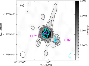
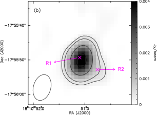
Figure 2: (a) The grey scale shows the high resolution radio continuum map of G12.42+0.50 at 1390 MHz with the contour levels 3, 6, 9, 18, 63, 150 and 172 times $\sigma$ ($\sigma\sim 29.7~{}\mu$Jy/beam). The beam size is $\sim 3.0^{\prime\prime}\times 2.4^{\prime\prime}$. Positions of R1 and R2 are also labelled. The contours of the 6 cm radio map are overlaid in cyan with the contour levels 3, 4, 6, 12, 21 and 24 $\sigma$ ($\sigma\sim 0.15$ mJy/beam) and the beam size is $\sim 2.2^{\prime\prime}\times 1.1^{\prime\prime}$. (b) The radio continuum map of G12.42+0.50 at 610 MHz with contour levels 3, 6, 18, 38 and 60 times $\sigma$ ($\sigma\sim 94~{}\mu$Jy/beam). The beam size is $\sim 7.6^{\prime\prime}\times 4.8^{\prime\prime}$. The positions of the two radio peaks detected in the 1390 MHz map is indicated by ‘x’. The restoring beams in the 1390 and 610 MHz bands are represented as open ellipses towards the bottom-left of each image and of the 6 cm map is represented as an open cyan ellipse towards the bottom-right in (a).

2.8 Molecular line data from MALT90 survey

To understand the gas kinematics in our region of interest, molecular line data were obtained from the MALT90 survey (Jackson et al., 2013; Foster et al., 2011). The survey, carried out using the ATNF Mopra 22-m telescope, has simultaneously mapped the transitions of 16 molecules near 90 GHz with a spectral resolution of $\rm 0.11~{}km~{}s^{-1}$. The Mopra Telescope is a 22-m single-dish radio telescope operated by The Commonwealth Scientific and Industrial Research Organisation’s Astronomy and Space Science division. The data reduction was performed using CLASS90 (Continuum and Line Analysis Single-dish Software), a GILDAS software (Grenoble Image and Line Data Analysis Software).

2.9 JCMT archival data

The molecular line data for the $J=3-2$ transition of $\rm{}^{12}CO$, $\rm{}^{13}CO$ and $\rm C^{18}O$ were downloaded from the archives of the Heterodyne Array Receiver Program (HARP) mounted on the James Clerk Maxwell Telescope (JCMT) operated by the East Asian Observatory. JCMT is a 15 m telescope and is the largest single-dish astronomical telescope which operates in the submillimetre wavelength region of the spectrum. HARP is a Single Sideband array receiver that can be tuned between 325 and 375 GHz and has an instantaneous bandwidth of $\sim$2 GHz and an Intermediate Frequency of 5 GHz. It comprises of 16 detectors laid out on a 4$\times$4 grid, with an on-sky projected beam separation of 30$\arcsec$. At 345 GHz the beam size is 14$\arcsec$ (Buckle et al., 2009).

2.10 TRAO observation

The molecular line data for the $J=1-0$ transition of $\rm{}^{13}CO$ was obtained from the Taeduk Radio Astronomy Observatory (TRAO). TRAO is a 14 m radio telescope with a single-horn receiver system operating in the frequency range of 86 to 115 GHz and is located on the campus of the Korea Astronomy and Space Science Institute (KASI) in Daejeon, South Korea. The main FWHM beam sizes for the $\rm{}^{12}CO~{}(1-0)$ and $\rm{}^{13}CO~{}(1-0)$ lines are 45$\arcsec$ and 47$\arcsec$ respectively. The system temperature ranges from 150 K, for $\rm 86-110$ GHz to 450 K, for 115 GHz and $\rm{}^{12}CO$ (Liu et al., 2018).

3 RESULTS

3.1 Emission from Ionized Gas

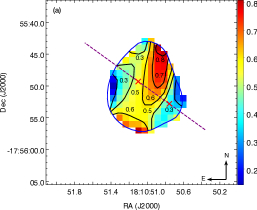
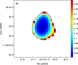
Figure 3: (a) Spectral index map of G12.42+0.50 between 1390 and 610 MHz. Black curves represent the spectral index levels. The blue contour shows the 5$\sigma$ ($\sigma\sim 0.4\times 10^{-4}$ Jy/beam) level of the 610 MHz map used to construct the spectral index map. The red ‘x’s mark the positions of the radio components, R1 and R2. The dashed purple line indicates the possible direction of the ionized jet. The spectral index varies from 0.3 to 0.7 along the possible jet axis. The error map is shown in (b). The errors involved are $\lesssim$ 0.15, barring a few pixels at the edges.

Table 4: Peak coordinates, peak and integrated flux densities, and deconvolved sizes of the components R1 and R2 associated with G12.42+0.50.

	Peak Coordinates		Deconvolved size ($\arcsec$$\times$$\arcsec$)			Peak flux (mJy/beam)			Integrated flux (mJy)
Component	RA (J2000)	Dec (J2000)	610 MHz	1390 MHz	5 GHz ∗	610 MHz	1390 MHz	5 GHz ∗	610 MHz	1390 MHz	5 GHz ∗
R1	18 10 51.10	-17 55 49.30	2.6 $\times$ 0.6	1.9 $\times$ 1.7	1.4 $\times$ 1.2	4.4	5.3	3.5	4.7	7.9	6.2
R2	18 10 50.76	-17 55 52.80	-	1.5 $\times$ 1.2 †	1.1 $\times$ 0.6 †	-	0.6	1.1	-	0.7	1.1

^† Upper limits which is half the FWHM of the restoring beam.

^∗ Values for R1 are from Urquhart et al. (2009) and for R2 they are estimated from the available map.

The radio continuum maps at 1390 and 610 MHz, probing the ionized gas emission associated with G12.42+0.50, are shown in Fig.  2. The 1390 MHz map reveals the presence of a linear structure in the north-east and south-west direction comprising of an extended emission with two distinct and compact components, labelled R1 and R2 in the figure. The component R1 is well resolved, whereas R2 seems to be barely resolved. In this figure, we also plot the contours of the high-resolution 6 cm (5 GHz) map obtained using VLA by Urquhart et al. (2009) as part of the RMS survey towards candidate massive YSOs. Both components are also visible in the 6 cm map. In comparison, the lower-resolution 610 MHz shows a single, almost spherical emission region with the peak position coinciding with R1. However, a discernible elongation is evident towards R2. In addition, the 1390 MHz map shows a narrow extension in the north-west and south-east direction. Given that the maps (especially 1390 MHz) have low level stripes in the said direction, it becomes difficult to comment on the genuineness of this feature.

Table 4 compiles the coordinates, peak and integrated flux densities of R1 and R2. The deconvolved sizes and integrated flux densities are estimated by fitting 2D Gaussians using the task IMFIT from Common Astronomy Software Application (CASA) (McMullin et al., 2007)). At 610 MHz, the components are not resolved so the values obtained are assigned to R1 and hence should be treated as upper limits. For the component R1, the 5 GHz values are quoted from Urquhart et al. (2009). As for the component R2, that is barely resolved in both 1390 MHz and 5 GHz maps, we have set an upper limit to its size at both frequencies. This is taken to be the FWHM of the respective restoring beams (Urquhart et al., 2009). Further, at 5 GHz, we take the peak flux density to be the same as the integrated flux density.

In order to get an in-depth knowledge of the nature of the observed radio emission, we generate the spectral index map using our 1390 and 610 MHz maps. The spectral index, $\alpha$, is defined as $S_{\nu}\propto\nu^{\alpha}$, where, $S_{\nu}$ is the flux density at frequency $\nu$. GMRT is not a scaled array, hence, each frequency is sensitive to different spatial scales. To circumvent this, we generate new maps in the uv range ($\rm 0.7-47K\lambda$) common to both frequencies. Keeping in mind the requirement of same pixel size and resolution, pixel and beam-matching is taken into account while generating the new maps. The spectral index map is then constructed using the task COMB in AIPS. Further, to ensure reliable estimates of the spectral index, we retain only those pixels with flux density greater than 5$\sigma$ ($\sigma$ being the rms noise of the map) in both maps. The generated spectral index map and the corresponding error map, which has the same resolution as that of the 610 MHz map ($\sim 7.6^{\prime\prime}\times 4.8^{\prime\prime}$), are presented in Fig. 3. As seen from the figure, the spectral index values vary between 0.3 and 0.9 with the estimated errors involved being less than $\sim$ 0.15, barring a few pixels at the edges. These values indicate that the region is dominated by thermal bremsstrahlung emission of varying optical depth (Rodriguez et al., 1993; Curiel et al., 1993; Kobulnicky & Johnson, 1999; Rosero et al., 2016). Moreover, spectral index values in the range of $0.4-0.9$ are also typically seen in regions associated with thermal jets (e.g. Panagia & Felli, 1975; Reynolds, 1986; Purser et al., 2016; Sanna et al., 2016). We will revisit these results obtained in a later section where we explore various scenarios to adequately explain the nature of the radio emission.

3.2 Emission from shock indicators

As discussed in the introduction, there is growing evidence in literature associating EGOs with MYSOs, notwithstanding the ongoing debate regarding their exact nature. Several mechanisms, like shocked emission in outflows, fluorescent emission or scattered continuum from MYSOs (Noriega-Crespo et al., 2004; De Buizer & Vacca, 2010; Takami et al., 2012), are invoked to identify the spectral carriers of the enhanced 4.5 $\rm\mu m$ emission. The picture of shocked emission from outflows suggests the spectral carriers to be molecular and atomic shock indicators like H₂ and [Fe ii] as well as the broad CO bandhead. All of these have distinct features within the 4.5 $\rm\mu m$ IRAC band. However, Simpson et al. (2012), while investigating the population of MYSOs in the G333.2-0.4 region, opine that the excess 4.5 $\rm\mu m$ could not be attributed to the H₂ lines as these would be too faint to be detected at this wavelength. Instead, they support a scattered continuum or the CO bandhead origin. From the $L$- and $M$-band spectra of two EGOs, De Buizer & Vacca (2010) show the H₂ line hypothesis to be consistent with one of them (G19.88-0.53), while in the other target (G49.27-0.34), the spectra shows only continuum emission. So far, spectroscopic studies of EGOs in the 4.5 $\rm\mu m$ and the NIR are few (De Buizer & Vacca, 2010; Caratti o Garatti et al., 2015; Onaka et al., 2016), thus keeping the debate on their nature ongoing. In the NIR domain, a few studies have focussed towards narrow-band imaging (Lee et al., 2012, 2013). Based on the UWISH2 survey images, Lee et al. (2012, 2013) present a complete H₂ line emission census of EGOs in the Northern Galactic Plane.

3.2.1 Narrow-band Imaging

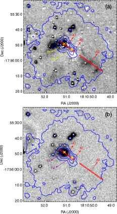
Figure 4: (a) Continuum subtracted H₂ image made using the UWISH2 survey data. (b) Continuum subtracted [Fe ii] image made using UKIRT-WFCAM observations towards G12.42+0.50. The positions of the identified radio components R1 and R2 are indicated. The blue contours represent the 4.5 $\rm\mu m$ emission with the levels 3, 60, 120, and 220$\sigma$ ($\sigma\sim 1.5$ MJy/sr). The red rectangles show the orientation of the slit and denote the apertures used for spectra extraction (see text in Section 3.2.2)

.

H₂ line emission towards G12.42+0.50 has been investigated in Lee et al. (2012). They ascribe the extended emission seen in the continuum-subtracted image to be the result of residuals of continuum subtraction rather than real H₂ line emission. In order to carefully scrutinize the NIR picture of G12.42+0.50, we revisit the H₂ line emission from images retrieved from the UWISH2 survey. In addition, we also probe the [Fe ii] line image which is a robust indicator of shocks as compared to the H₂ lines (Shinn et al., 2014).

Following the procedure outlined in Section 2.2.2 we construct the continuum subtracted H₂ and [Fe ii] line images which are presented in Fig. 4. In the continuum-subtracted H₂ image, the morphology is similar to that obtained by Lee et al. (2012). An extended emission is seen towards the peak of the 4.5 $\rm\mu m$ emission coinciding with the location of the the radio component R1. Ideally a narrow-band continuum filter should enable a better continuum subtraction but in the absence of the same, we have ensured PSF matching and proper scaling of the broad $K$-band image. Contrary to the suggestion by Lee et al. (2012), we believe that the extended H₂ line emission detected in the continuum-subtracted image is genuine. This finds strength in the spectra obtained and discussed in the next section. In addition, diffuse line emission is seen towards the north-east and east of R1 as well towards the south-west. The continuum-subtracted [Fe ii] image shows a weak, extended emission coinciding with the brighter part of the H₂ line emission.

3.2.2 NIR spectroscopy

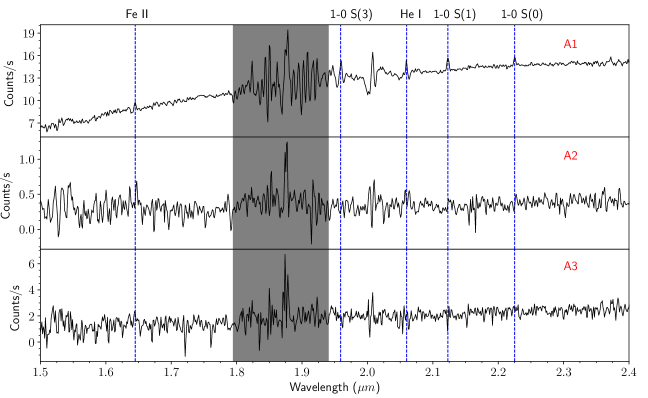
Figure 5: The $HK$ spectrum of G12.42+0.50 extracted over the apertures A1, A2 and A3. The aperture A1 covers the radio component R1 and the extended H₂ emission seen towards the north-east, A2 covers the second radio component R2 and A3 samples the detached, extended emission seen towards the south-west. The shaded area marks the region of poor sky transparency. The identified spectral lines along aperture A1 are marked over the spectrum with the details given in Table 5. No emission lines above the noise level are detected in the spectra extracted over A2 and A3.

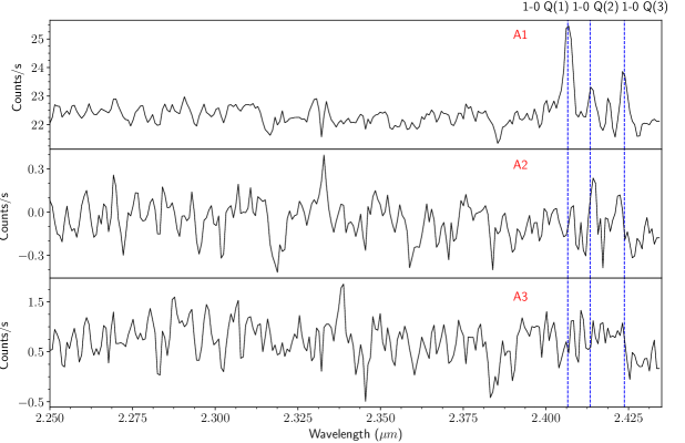
Figure 6: The $KL$ spectrum of G12.42+0.50 extracted over the apertures A1, A2 and A3. The regions covered by all the three apertures are the same as given in Fig. 5. The identified spectral lines along aperture A1 are marked over the spectrum with the details given in Table 5. No emission lines above the noise level are detected in the spectra extracted over A2 and A3.

Table 5: Lines detected in the spectra extracted from aperture A1 towards G12.42+0.50.

Line	Wavelength ($\mu$m)
[Fe ii]	1.644
H2 1-0 S(3)	1.958
He I	2.059
H2 1-0 S(1)	2.122
H2 1-0 S(0)	2.224
H2 1-0 Q(1)	2.407
H2 1-0 Q(2)	2.413
H2 1-0 Q(3)	2.424

As is clear from earlier discussions, studies towards identifying the spectral carriers of the 4.5 $\rm\mu m$ emission are crucial in understanding the nature of EGOs and confirming their association with MYSOs. Given the lack of sensitive spectrometers in the 4.5 $\rm\mu m$ region, spectroscopy in the NIR becomes indispensable. We probe G12.42+0.50 with NIR spectroscopy to understand further the results obtained from narrow-band imaging. From the continuum-subtracted line images shown in Fig. 4 and the UKIDSS $K$-band image shown in Fig. 1, presence of faint nebulosity around the peak position (that coincides with the 4.5 $\rm\mu m$ peak) and towards the south-west is clearly visible. The slit orientation shown in Fig. 4 ensures that the regions harbouring the radio components and the extended H₂ line emission towards the north-east of the peak and the detached elongated nebulosity towards the south-west are probed.

The $HK$ spectra extracted over the three identified apertures (marked in Fig. 4) are shown in Fig. 5. The top-panel of Fig. 5 shows the spectrum over aperture A1 with the line details listed in Table 5. This aperture covers the radio component R1 and portions of the extended H₂ emission seen towards the north-east of the 4.5 $\rm\mu m$ peak. The spectrum shows clear detection of three emission lines of molecular H₂ with the most prominent feature being the $\rm 1-0S(1)$ line at 2.122 $\rm\mu m$. No H₂ line is detected in the blue part ($\rm 1.5-1.8~{}\mu m$) of the spectrum but there is a weak [Fe ii] line detected at 1.644 $\rm\mu m$ These lines of H₂ and [Fe ii] are commonly observed in outflows/jets. In addition, He I at 2.059 $\rm\mu m$ is also seen in the extracted spectrum. Apart from the emission lines, the continuum slope is seen rising towards the red thus, indicating a highly reddened source. Fig. 5 also plots the extracted spectra over the apertures A2 and A3 in the middle and lower panels, respectively. Aperture A2 covers the second radio component R2 and aperture A3 samples the detached, extended emission seen towards the south-west. No emission lines above the noise level are detected in these and the spectra displayed are flat.

In Fig. 6, we present the extracted spectra in the $KL$ band. The displayed spectra has been truncated at 2.45 $\rm\mu m$ due to poor signal-to-noise ratio owing to less than optimal sky transparency. In aperture A1, three additional emission lines of molecular H₂ are prominent. The other two apertures do not show the presence of any spectral feature. The detected lines are listed in Table 5.

The observed H₂ line emissions seen in the spectra of G12.42+0.50 can be attributed to either thermal or non-thermal excitation. The thermal emission mostly originates from shocked neutral gas in outflows/jets that are heated up to a few 1000 K, whereas, the non-thermal emission is understood to be due to UV fluorescence by non-ionizing UV photons. These two competing mechanisms populate different energy levels thus yielding different line ratios (Davis et al., 2003; Caratti o Garatti et al., 2015; Veena et al., 2016). UV fluorescence excites higher vibrational levels. The H₂ lines detected in G12.42+0.50 originate from the upper vibrational level, $\nu=1$ suggesting a low level of excitation. The absence of high vibrational state transitions supports the shock-excited origin of the detected lines. Lack of fluorescent H₂ line emission in G12.42+0.50 may also be due to veiling of UV photons from the central star due to high extinction. Nevertheless, given the association with an outflow source, shock-excited origin is most likely the case.

3.3 Emission from the dust component

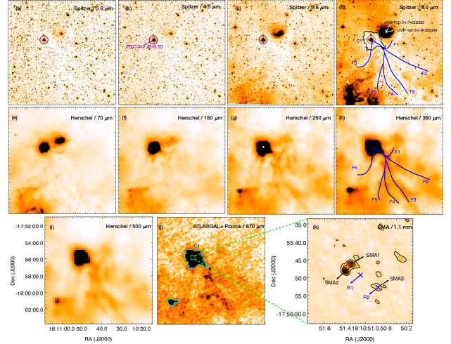
Figure 7: Dust emission in the region associated with G12.42+0.50 at the mid- and far-infrared wavelengths ($\rm 3.6~{}\mu m-1.1~{}mm$). All the images from (a)$-$(j) have the same field of view. Skeletons of six clearly identified filaments are overlaid on the 8.0 and 350 $\rm\mu m$ maps. The position of the EGO, G12.42+0.50 is shown within a purple circle on the 3.6, 4.5, 5.8 and 8.0 $\rm\mu m$ IRAC maps. The location of the two infrared dust bubbles (MWP1G012417+005383 and MWP1G012419+005399) are indicated by white ‘x’s on the 8.0 $\rm\mu m$ map, (d). (d) and (j) show the retrieved aperture of clump C1. Another clump detected towards south-east of G12.42+0.50 is shown in the 870 $\rm\mu m$ map, (j). (k) shows the SMA 1.1 mm map with the contour levels 3, 12, 21, 30 and 39 times $\sigma$ ($\sigma\sim 3$ mJy/beam). The blue ‘x’s on the 1.1 mm map mark the positions of the radio components R1 and R2.

The dust emission at MIR and FIR wavelengths sampled in the IRAC, Hi-Gal, ATLASGAL-Planck and SMA wavelengths (3.6 $\rm\mu m$$-$1.1 mm) in the region associated with G12.42+0.50 is shown in Fig. 7. In the IRAC bands, various emission mechanisms come into play and contribute towards the warm dust component (Watson et al., 2008). Thermal emission from the circumstellar dust heated by the stellar radiation and emission from the UV excited polycyclic aromatic hydrocarbons in the Photo Dissociation Regions are known to be the dominant contributors. In the shorter IRAC wavelengths (3.6, 4.5 $\rm\mu m$), where mostly the stellar sources are sampled, emission from the stellar photosphere would also be appreciable. Apart from this, shock-excited H₂ line emission and diffuse emission in the Br$\alpha$ and Pf$\beta$ lines would also exist. Further, in case of H ii regions, one expects significant contribution from the Ly$\alpha$ heated dust (Hoare, Roche & Glencross, 1991). The morphology in the IRAC bands is similar and the emission becomes more prominent at 8.0 $\rm\mu m$. Dark filamentary features (bright in the negative images shown) are seen in silhouette towards the south-west in the 8.0 $\rm\mu m$ map. The skeletons of the six clearly identified filamentary features are overlaid on the 8.0 $\rm\mu m$ map. In addition, an extended emission feature is seen towards the north-west of G12.42+0.50, being prominent in the 5.8, 8.0, and 70 $\rm\mu m$ images. Two infrared dust bubbles (MWP1G012417+005383 and MWP1G012419+005399) are found to be associated with this feature and are marked in Fig. 7(d). No further literature is available on these bubbles so we drop them in further discussion.

As we move towards the longer wavelengths, cold dust emission associated with G12.42+0.50 becomes enhanced and more extended. From the ATLASGAL-Planck combined 870 $\rm\mu m$ map, we identify two clumps using the 2D Clumpfind algorithm (Williams, de Geus & Blitz, 1994) with 2$\sigma$ ($\sigma$ = 0.3 Jy/beam) threshold and optimum contour levels. The apertures of the identified clumps are overlaid on the 870 $\rm\mu m$ map in Fig. 7(j). While one of the clumps, hereafter C1, is associated with G12.42+0.50, another clump lies towards the south-east of G12.42+0.50 at an angular distance of $\sim 6^{\prime}$. From the $\rm H^{13}CO^{+}$ molecular line data (Section 3.4), we estimate the LSR velocity of this clump to be $\rm 31.5~{}km~{}s^{-1}$. Comparing this with the estimated LSR velocity of G12.42+0.50 ($\rm 18.3~{}km~{}s^{-1}$), it is unlikely that the clump has any association with G12.42+0.50. The identified filaments now appear in emission and are shown on the 350 $\rm\mu m$ map. Interestingly, these filaments seem to converge towards clump C1. As mentioned in the introduction, the morphology has an uncanny resemblance to a hub-filament structure, detailed discussion of which is presented in Section 4.2.3. Furthermore, in the high-resolution 1.1 mm SMA map, the inner region of the cold dust clump, C1 associated with G12.42+0.50 is seen to harbour two, dense and bright compact cores labelled on the map as SMA1 and SMA2. Additionally, a few bright emission knots are detected in the SMA map including the one highlighted as SMA3 which coincides with the radio component R2.

3.3.1 Properties of SMA cores

From the SMA 1.1 mm map shown in Fig. 7(k), SMA1 and SMA2 show up as dense, compact cores possibly in a binary system. SMA3, on the other hand, looks more like a clumpy region of density enhancement. Following the method described by Kauffmann et al. (2008) the masses of the SMA components are computed using the equation

$$M = \displaystyle 0.12\,M_{\odot}\left({\rm e}^{1.439(\lambda/{\rm mm})^{-1}(T/{\rm 10~{}K})^{-1}}-1\right)$$ (2)

$$\displaystyle\left(\frac{\kappa_{\nu}}{0.01\rm~{}cm^{2}~{}g^{-1}}\right)^{-1}\left(\frac{F_{\nu}}{\rm Jy}\right)\left(\frac{d}{\rm 100~{}pc}\right)^{2}\left(\frac{\lambda}{\rm mm}\right)^{3}$$

where the opacity is

$$\kappa_{\nu}=0.1({\nu}/\textrm{1000~{}GHz})^{\beta}~{}{\rm cm}^{2}{\rm g}^{-1}$$ (3)

$\beta$ is the dust emissivity spectral index which is fixed at 2.0 (Hildebrand, 1983; Beckwith et al., 1990; André et al., 2010). $F_{\nu}$ is the integrated flux density of each component, $d$ is the distance to the source and $\lambda$ is the wavelength taken as 1.1 mm. The temperature, $T$ is taken to be 26.8 K for SMA1 and SMA2 and 22.7 K for SMA3, from their positions in the dust temperature map (Section 3.3.3). The peak positions and flux densities, integrated flux densities, the deconvolved sizes and the masses of the of the 1.1 mm SMA cores are presented in Table 6. The deconvolved sizes and integrated flux densities of the cores are evaluated by fitting 2D Gaussians to each component using the 2D fitting tool of CASA viewer. From the mass and size estimates, SMA1 and SMA2 qualify as potential high-mass star forming cores satisfying the criterion, $m(r)>870{\rm M_{\odot}}(r/\rm pc)^{1.33}$ (Kauffmann et al., 2010b).

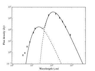
Figure 8: Spectral energy distribution of the dust core associated with G12.42+0.50 in the wavelength range of 3.6 to 870 $\rm\mu m$. Assumed 15% errors are indicated. The solid curve represents the best fit two-component model with a warm component at 183 K and a cold envelope at 25 K.

Table 6: Physical parameters of the 1.1 mm continuum emission near G12.42+0.50.

Component	Peak position		Deconvolved size	Integrated flux	Peak flux	Mass
	RA (J2000) $({{}^{h}}~{}{{}^{m}}~{}{{}^{s}})$	Dec (J2000) $(\degree~{}\arcmin~{}\arcsec)$	($\arcsec$$\times$$\arcsec$)	(mJy)	(mJy/beam)	(M⊙)
SMA1	18 10 51.3	-17 55 46.3	1.4$\times$0.5	190	109	14.8
SMA2	18 10 51.4	-17 55 48.1	1.3$\times$0.4	221	136	17.2
SMA3	18 10 50.8	-17 55 52.8	1.5$\times$0.7	57	34	5.5

Table 7: Integrated flux densities of the dust core associated with G12.42+0.50.

Wavelength ($\rm\mu m$)	3.6	4.5	5.8	8.0	12.13	14.65	70	160	250	350	500	870
Flux density (Jy)	0.6	0.9	3.3	8.4	57.7	129.8	1942.6	2575.5	1140.7	535.3	182.5	35.9

Table 8: Derived physical parameters of identified clumps associated with G12.42+0.50. The peak position, radius, mean temperature and column density, total column density, mass, and volume number density of the identified clumps are listed.

Clump	Peak position		Radius	Mean $T_{d}$	Mean $N(H_{2})$	$\Sigma N(H_{2})$	Mass	Number density, $n(H_{2})$
	$\rm\alpha(J2000)~{}({{}^{h}}~{}{{}^{m}}~{}{{}^{s}})$	$\rm\delta(J2000)~{}(\degree~{}\arcmin~{}\arcsec)$	(pc)	(K)	(${\sc 10^{22}}$ cm-2)	($10^{23}$ cm-2)	(M⊙)	($10^{3}$ cm-3)
C1	18 10 49.64	-17 55 59.40	0.8	19.9$\pm$1.9	3.3$\pm$0.9	23.2	1375	10.4
C2	18 10 42.75	-17 57 08.92	0.3	16.1$\pm$0.4	1.2$\pm$0.1	1.0	59	10.7
C3	18 10 36.91	-17 55 02.54	0.4	17.1$\pm$0.8	0.7$\pm$0.1	1.5	92	4.2
C4	18 10 37.83	-17 58 04.57	0.4	16.7$\pm$0.7	0.9$\pm$0.1	2.1	127	4.9
C5	18 10 27.03	-17 58 17.79	0.4	17.7$\pm$0.9	0.7$\pm$0.1	1.1	66	4.4
C6	18 10 23.08	-17 59 55.48	0.4	18.1$\pm$0.9	0.7$\pm$0.1	1.2	70	4.3
C7	18 10 19.16	-17 59 27.19	0.2	18.2$\pm$0.8	0.7$\pm$0.1	0.4	24	7.2
C8	18 10 43.71	-17 58 04.98	0.5	15.8$\pm$0.6	1.2$\pm$0.2	3.6	214	6.0
C9	18 10 38.76	-18 00 24.61	0.2	15.6$\pm$0.7	1.2$\pm$0.2	0.7	41	11.1
C10	18 10 35.81	-18 00 52.40	0.3	16.0$\pm$0.8	1.1$\pm$0.2	0.9	55	9.5
C11	18 10 43.67	-18 00 24.95	0.7	16.3$\pm$0.8	1.0$\pm$0.2	6.0	359	3.5
C12	18 10 38.73	-18 02 02.59	0.2	16.3$\pm$1.1	0.8$\pm$0.2	0.5	29	9.7

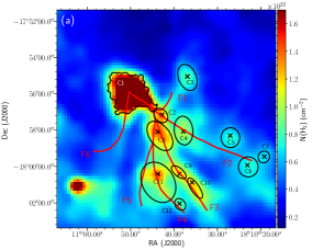
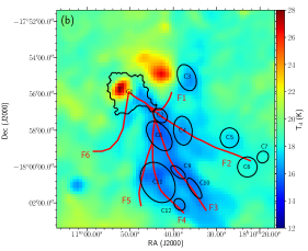
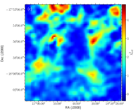
Figure 9: (a) Column density, (b) Temperature and (c) Reduced ${\chi^{2}}$ maps towards G12.42+0.50 generated using the Herschel FIR data and the ATLASGAL-Planck data. The Clumpfind retrieved clump,C1 and the visually identified clumps from the column density map are marked on the maps. The ‘x’s mark the positions of the peak column densities of each clump in the column density map. Skeletons of the filaments identified from the 8.0 $\rm\mu m$ map is overlaid on the column density and temperature maps.

3.3.2 SED modelling of C1

In an attempt to understand the properties of the dust clump (C1) associated with G12.42+0.50, we model the infrared flux densities with a two-component modified blackbody using the following functional form (Lis & Menten, 1998)

$$S_{\nu}=[\Omega_{1}\;{\it a}\;B_{\nu}(T_{1})+\Omega_{2}\;(1-{\it a})\;B_{\nu}(T_{2})](1-e^{-\tau_{\nu}})$$ (4)

where

$$\tau_{\nu}=\mu_{H_{2}}m_{H}\kappa_{\nu}N(H_{2})$$ (5)

where $S_{\nu}$ is the integrated flux density of C1, $\Omega_{1}$ and $\Omega_{2}$ are the solid angles subtended by the apertures used for estimating the flux densities at the FIR and MIR wavelengths, respectively. $a$ is the ratio of optical depth in the warmer component to the total optical depth, $B_{\nu}(T_{1})$ and $B_{\nu}(T_{2})$ are the blackbody functions at dust temperatures $T_{1}$ and $T_{2}$, respectively, $\mu_{H_{2}}$ is the mean molecular weight (taken as 2.8; Kauffmann et al., 2008), $m_{H}$ is the mass of hydrogen atom, $\kappa_{\nu}$ is the dust opacity and $N(H_{2})$ is the hydrogen column density. For opacity, we assume the function $\kappa_{\nu}=0.1({\nu}/\rm 1000~{}GHz)^{\beta}~{}cm^{2}~{}g^{-1}$, where $\beta$ is the dust emissivity spectral index for which, a value of 2.0 is adopted as in the previous section.

In addition to the Spitzer-IRAC, Herschel and ATLASGAL wavebands, we have also included flux densities from the MSX survey at 12.13 and 14.65 $\rm\mu m$ to constrain the model in the MIR wavelength. The integrated flux densities of the dust clump at the MIR wavelengths are measured within the area defined by the 4$\sigma$ contour level of the 8.0 $\rm\mu m$ image (274 arcsec²) and longward of 70 $\rm\mu m$, the integration is done over the area defined by the Clumpfind aperture for C1 (13720 arcsec²). Background emission is estimated using the same apertures on nearby sky region (visually scrutinized to be smooth) and subtracted. Estimated flux densities are listed in Table 7. Schuller et al. (2009); Launhardt et al. (2013) use a conservative 15% uncertainty in the flux densities of the Herschel bands. We adopt the same value here for all the bands. Model fitting is carried out using the non-linear least square Levenberg-Marquardt algorithm with $T_{1}$, $T_{2}$, $N(H_{2})$ and $a$ taken as free parameters. The best fit temperature values are 25.0$\pm$1.0 K (cold) and 183.2$\pm$12.0 K (warm), respectively. The model fit also gives an estimate of the hydrogen column density, $N(H_{2})=\rm 2.1\times 10^{22}~{}cm^{-2}$. This result shows that the dust clump in G12.42+0.50 consists of an inner warm component surrounded by an extended outer, cold envelope traced mostly by the FIR wavelengths. It should be noted here that we have excluded the data points below 8.0 $\rm\mu m$ while fitting the model. This is because the emission at 4.5 and 5.8 $\rm\mu m$ may largely be dominated by shock excitation and the 3.6 $\rm\mu m$ emission may arise from even hotter components. The SED and the best fit modified blackbody are shown in Fig. 8. The bolometric luminosity estimated from the two-component SED model over $8.0-870$ $\rm\mu m$ is $2.8\times 10^{4}$ L_⊙. It is a factor of 1.6 higher to that obtained by Vutisalchavakul & Evans (2013), who use the IRAS band flux densities. However, our values are in fair agreement to the estimate of $\rm 3.2\times 10^{4}$ L_⊙ (Osterloh, Henning & Launhardt, 1997) where flux densities between $\rm 2.1-1.3~{}mm$ are included.

3.3.3 Nature and distribution of cold dust emission

We probe the nature of the cold dust associated with G12.42+0.50, using the Herschel FIR bands which cover the wavelength range ($\rm 160-500$ $\rm\mu m$) and the combined ATLASGAL-Planck data at 870 $\rm\mu m$. The dust temperature and the line-of-sight average molecular hydrogen column density maps are generated by a pixel-by-pixel modified single-temperature blackbody model fitting. While fitting the model, we assume the emission at these wavelengths to be optically thin. Following the discussion in several papers (Peretto et al., 2010; Anderson et al., 2010; Battersby et al., 2011; Das et al., 2018), we exclude the 70 $\rm\mu m$ data point as the optically thin assumption would not hold. In addition, the emission here would have significant contribution from the warm dust component thus modelling with a single-temperature blackbody would over-estimate the derived temperatures. Given this, the model fitting is done with only five points which lie on the Rayleigh-Jeans tail.

The first step towards the generation of the temperature and column density maps is to have the maps from SPIRE, PACS and ATLASGAL-Planck in the same units. The units of the SPIRE map which is in MJy sr^-1 is converted to Jy pixel^-1 which is the unit for the 160 $\rm\mu m$ PACS map. Similarly, the ATLASGAL-Planck map that has the unit of Jy beam^-1 is also converted to Jy pixel^-1. The maps are at different resolutions and pixel sizes. The pixel-by-pixel routine makes it mandatory to convolve and regrid the maps to a common resolution and pixel size of 36$\arcsec$ and 14$\arcsec$, respectively which are the parameters of the 500 $\rm\mu m$ map (as it has the lowest resolution). Convolution kernels are taken from Aniano et al. (2011) for the Herschel maps. Since no pre-made convolution kernel is available for the ATLASGAL-Planck map, we use a Gaussian kernel. These preliminary steps are carried out using the software package, HIPE

The maps include sky/background emission which is a result of the cosmic microwave background and the diffuse Galactic emission. In order to correct for the flux offsets due to this background contribution, we select a relatively uniform and dark region (free of bright, diffuse or filamentary emission) at a distance of $\sim$0.25° from G12.42+0.50. The same region is used for background subtraction in all the five bands. Using the method described in several papers (Battersby et al., 2011; Launhardt et al., 2013; Ramachandran et al., 2017; Das et al., 2017, 2018) the background values, ${I_{bg}}$ are estimated to be -2.31, 2.15, 1.03, 0.37 and 0.08 Jy pixel^-1 at 160, 250, 350, 500 and 870 $\rm\mu m$, respectively. The negative flux value at 160 $\rm\mu m$ is due to the arbitrary scaling of the PACS images.

To probe an extended area encompassing G12.42+0.50 and the related filaments, we select a 12.8′$\times$12.8′ region centred at $\rm\alpha_{J2000}=18^{h}10^{m}41.8^{s},\delta_{J2000}=-17\degree 57\arcmin 23\arcsec$. The model fitting algorithm was based on the following formulation (Ward-Thompson & Robson, 1990; Battersby et al., 2011; Launhardt et al., 2013; Mallick et al., 2015):

$$S_{\nu}(\nu)-I_{bg}(\nu)=B_{\nu}(\nu,T_{d})\;\Omega\;(1-e^{-\tau_{\nu}})$$ (6)

where $\tau_{\nu}$ is given by Eqn. 5, $S_{\nu}$ is the observed flux density, $B_{\nu}(\nu,T_{d})$ is the Planck function, $T_{d}$ is the dust temperature, $\Omega$ is the solid angle in steradians, from where the flux is measured (solid angle subtended by a $\rm 14^{\prime\prime}\times 14^{\prime\prime}$ pixel) and the rest of the parameters are the same as used in the previous section. Following the same procedure discussed in Section 3.3.2, SED modelling for each pixel is carried out keeping the dust temperature, $T_{d}$ and column density, $N(H_{2})$ as free parameters. The dust temperature and column density maps generated are displayed in Fig. 9 along with the reduced ${\chi^{2}}$ map. The reduced ${\chi^{2}}$ map indicates that the fitting uncertainties are small with a maximum value of 4 towards the bright central emission where the 250 $\rm\mu m$ image (Fig. 7(e)) has a few bad pixels. The column density map reveals a dense, bright region towards clump, C1 that envelopes G12.42+0.50. Also clear is increased density along the filamentary structures identified in Section 3.3. The apertures of the clump C1 identified from the 870 $\rm\mu m$ is overlaid on the maps. Using $3\times 3$ pixel grids, local column density peaks are identified above 3$\sigma$ threshold ($\rm\sigma=2.3\times 10^{21}~{}cm^{-2}$). 11 additional clumps were thus identified located within the 3$\sigma$ contour. Subsequent to this, a careful visual inspection is done and ellipses are marked to encompass most of the clump emission.

Two high-temperature regions are seen in the dust temperature map coinciding with G12.42+0.50 and the two bubbles discussed earlier. The warmest temperature in the map is found to be 28.6 K and is located a pixel to the north-east of SMA1, SMA2 and peak position of R1. The mean dust temperature and column density of C1 is found to be 19.9 K and 3.3$\rm\times 10^{22}~{}cm^{-2}$, respectively. It has to be noted here that the mean temperature we obtain here is less than the temperature of the cold component we estimate from the two-component model by $\rm\sim 5~{}K$. This is because, unlike the two-component modelling, here we do not include the emission at 70 $\rm\mu m$. Similarly the column density we obtain here is greater than the column density estimated using the two-component fit by a factor of $\sim 1.6$. A striking feature noticed is the distinct low dust temperatures along the filaments.

3.3.4 Properties of cold dust clumps

Several physical parameters of the identified clumps are derived. The enclosed area within the Clumpfind retrieved aperture of C1 is used to determine the effective radius, $\rm r=(A/\pi)^{0.5}$ (Kauffmann et al., 2010a), where A is the area. For the visually identified clumps ($\rm C2-C12$), the effective radius is taken to be the geometric mean of the semi-major and semi-minor axes of the ellipses bounding the clumps. From the derived column density values, we estimate the mass of the dust clumps using the following expression

$$M_{\rm C}=\mu_{H_{2}}m_{H}A_{\rm pixel}\Sigma N(H_{2})$$ (7)

where $A_{\rm pixel}$ is the area of a pixel in $\rm cm^{2}$, $\mu_{H_{2}}$ is the mean molecular weight (2.8), $m_{H}$ is the mass of hydrogen atom. The volume number density of the clump is estimated using the expression,

$$n_{(H_{2})}=\frac{3~{}M_{\rm C}}{4\pi R^{3}\mu m_{H}}$$ (8)

The peak position, radius, mean temperature and column density, integrated column density, mass, and volume number density of the identified clumps are listed in Table 8. The clump enclosing G12.42+0.50, C1 is the largest and most massive clump having a radius 0.8 pc, column density $\rm 3.3\times 10^{22}~{}cm^{-2}$ and mass 1375 M_⊙. He et al. (2015) derives the radius, column density and mass of the clump associated with G12.42+0.50 to be 0.57 pc, $\rm 1.3\times 10^{23}~{}cm^{-2}$ and 724 M_⊙, respectively. Apart from a larger size estimated by us, the other factors contributing to this difference in the estimated values of mass and column density are the different opacity and dust temperature values adopted by He et al. (2015).

3.4 Molecular line emission from G12.42+0.50

Table 9: Details of the detected molecular line transitions towards the clump, C1 enveloping G12.42+0.50. The details are extracted from Table 2 of Miettinen (2014) and Table 2 of Foster et al. (2011).

Transition	Comments
H13CO${}^{+}~{}(1-0)$	six hyperfine (hf) components; high-density and ionization tracer
$\rm C_{2}H~{}(1-0)~{}3/2-1/2$	three hf components; photodissociation region tracer
HCN $(1-0)$	three hf components; high-density and infall tracer
$\rm HCO^{+}~{}(1-0)$	high-density, infall, kinematics and ionization tracer
HNC $(1-0)$	three hf components; high-density and cold gas tracer
$\rm HC_{3}N~{}(10-9)$	six hf components; High-density and hot-core tracer
$\rm N_{2}H^{+}~{}(1-0)$	15 hf components, seven have a different frequency; high density and CO-depleted gas tracer

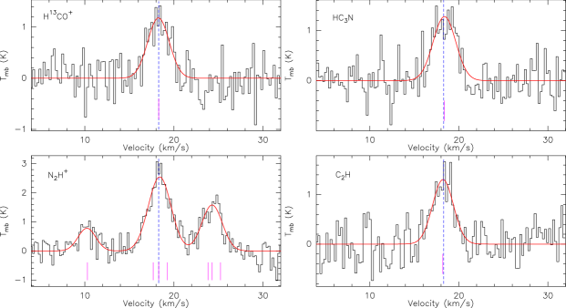
Figure 10: Spectra of the optically thin molecular lines ($\rm H^{13}CO^{+}$, $\rm HC_{3}N$, $\rm C_{2}H$ and $\rm N_{2}H^{+}$) associated with G12.42+0.50 obtained from the MALT90 survey. The spectra are extracted towards the peak of the 870 $\rm\mu m$ ATLASGAL emission. The dashed blue line indicates the LSR velocity, $\rm 18.3~{}km~{}s^{-1}$, estimated from the the optically thin $\rm H^{13}CO^{+}$ line. The magenta lines indicate the location of the hyperfine components for each transition.

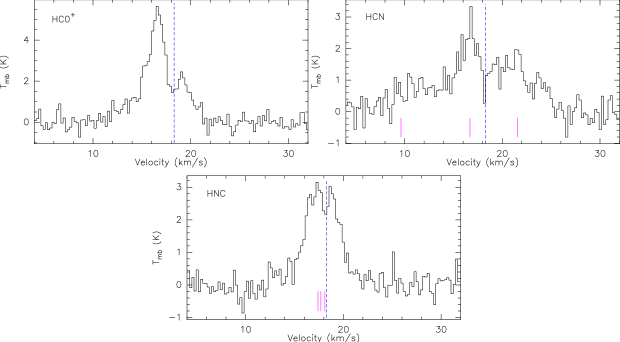
Figure 11: Same as Fig. 10 but for the optically thick transitions of $\rm HCO^{+}$, HCN, and HNC.

Table 10: Parameters of the optically thin molecular transitions detected towards G12.42+0.50. The line width ($\Delta V$), main beam temperature ($\rm T_{mb}$) and velocity integrated intensity ($\rm\int T_{mb}$) are obtained from the hfs fitting method of CLASS90 for all the molecules except for $\rm H^{13}CO^{+}$, for which a single Gaussian profile is used to fit the spectrum. The column densities ($N$) of molecules are estimated using RADEX, and their fractional abundances ($x$) are determined using the mean H₂ column density of the clump, C1.

Transition	$\Delta V$	$\rm T_{mb}$	$\rm\int T_{mb}$	$N$	$x$
	($\rm km~{}s^{-1}$)	(K)	($\rm K~{}km~{}s^{-1}$)	($\rm 10^{14}~{}cm^{-2}$)	($10^{-9}$)
$\rm H^{13}CO^{+}$	2.9	1.2	3.6	0.1	0.3
$\rm N_{2}H^{+}$	3.2	2.5	8.5	4.1	12.4
$\rm HC_{3}N$	3.0	1.3	4.1	1.4	4.2
$\rm C_{2}H$	2.7	1.3	3.8	5.5	16.7

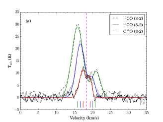
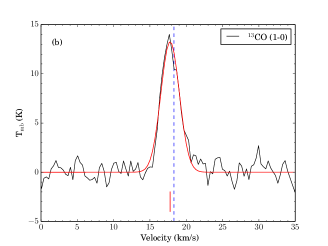
Figure 12: (a) Rotational transition lines of isotopologues of the $\rm CO~{}(3-2)$ observed towards G12.42+0.50 fitted with double Gaussians. The spectra of $\rm{}^{12}CO$, $\rm{}^{13}CO$ and $\rm C^{18}O$ are boxcar-smoothed by three, eight and eleven channels which correspond to velocity smoothing of 1.2, 3.4 and $\rm 4.6~{}km~{}s^{-1}$, respectively. The fit to the $\rm{}^{12}CO$ spectrum is depicted in green, $\rm{}^{13}CO$ in blue and $\rm C^{18}O$ in red. The dashed magenta line corresponds to the LSR velocity, $\rm 18.3~{}km~{}s^{-1}$. The positions of the red- and blueshifted components are indicated in green, blue and red lines for $\rm{}^{12}CO$, $\rm{}^{13}CO$ and $\rm C^{18}O$ lines respectively. (b) Spectrum of the $J=1-0$ transition of $\rm{}^{13}CO$ obtained from TRAO. The Gaussian fit to the spectrum is sketched in red. The dashed blue line corresponds to the LSR velocity. The spectrum shows a blue shifted single peak, indicated by a red line. The red and blue lobes are not resolved, probably due to larger beam size of TRAO compared to JCMT.

Table 11: The retrieved parameters, peak velocities, velocity widths and peak fluxes of the molecular transitions $\rm{}^{12}CO~{}(3-2)$, $\rm{}^{13}CO~{}(3-2)$, $\rm C^{18}O~{}(3-2)$ and $\rm{}^{13}CO~{}(1-0)$ towards G12.42+0.50. R and B in parentheses denote the red and blueshifted components.

Transition	$V$		$\Delta V$		$\rm T_{mb}$
	($\rm km~{}s^{-1}$)		($\rm km~{}s^{-1}$)		(K)
$\rm{}^{12}CO~{}(3-2)$	21.0 (R)	15.8 (B)	2.8 (R)	3.7 (B)	10.7 (R)	29.1(B)
$\rm{}^{13}CO~{}(3-2)$	19.9 (R)	16.6 (B)	2.0 (R)	3.9 (B)	7.7 (R)	21.9 (B)
$\rm C^{18}O~{}(3-2)$	19.3 (R)	17.4 (B)	1.2 (R)	2.4 (B)	6.6 (R)	11.2 (B)
$\rm{}^{13}CO~{}(1-0)$	17.8		3.0		13.3

The molecular line emission provides information on the kinematics and chemical structure of a molecular cloud in addition to throwing light on its evolutionary stage. Data from the MALT90 survey, JCMT archives and observation from TRAO are used to probe these aspects in the star forming region associated with G12.42+0.50.

Of the 16 molecules covered by the MALT90 survey, 7 molecular species, namely $\rm HCO^{+}$, $\rm H^{13}CO^{+}$, HCN, HNC, $\rm C_{2}H$, $\rm N_{2}H^{+}$ and $\rm HC_{3}N$ are detected towards the clump C1 enveloping G12.42+0.50. The details of the detected transitions taken from Miettinen (2014) and Foster et al. (2011) are listed in Table 9. Miettinen (2014) also gives an excellent review on the physical conditions and environment required for the formation of these species. The spectrum of each molecule is extracted towards the 870 $\rm\mu m$, ATLASGAL emission peak. The spectra of the optically thin molecular species, $\rm H^{13}CO^{+}$, $\rm C_{2}H$, $\rm N_{2}H^{+}$ and $\rm HC_{3}N$, are shown in Fig. 10 and the spectra of the optically thick molecular species, $\rm HCO^{+}$, HCN and HNC, are plotted in Fig. 11. We use the hyperfine structure (hfs) method of CLASS90 to fit the observed spectra for the optically thin transitions of $\rm C_{2}H$, $\rm N_{2}H^{+}$ and $\rm HC_{3}N$. Since the molecule $\rm H^{13}CO^{+}$ has no hyperfine components, a single Gaussian profile is used to fit the spectrum. The Gaussian fit yields a LSR velocity of $\rm 18.3~{}km~{}s^{-1}$, which is consistent with the value estimated using the $\rm N_{2}H^{+}$ line of the same survey ($\rm 18.3~{}km~{}s^{-1}$; Yu & Wang 2015). The fit to the spectra are indicated by solid red line, and the LSR velocity and the location of the hyperfine components are indicated by the dashed blue and solid magenta lines, respectively in Fig. 10. The retrieved line parameters that include the peak velocity ($V_{\rm LSR}$), line width ($\Delta V$), main beam temperature ($\rm T_{mb}$) and the velocity integrated intensity ($\rm\int T_{mb}$) are tabulated in Table 10. Beam correction is applied to the antenna temperature to obtain the main beam temperature using the equation, $\rm T_{mb}=T_{A}/\eta_{mb}$ (Rathborne et al., 2014), where $\rm\eta_{mb}$ is assumed to be 0.49 (Ladd et al., 2005) for the MALT90 data.

To estimate the column density of these transitions, we use RADEX, a one dimensional non-local thermodynamic equilibrium radiative transfer code (van der Tak et al., 2007). The input parameters to RADEX include the peak main beam temperature, background temperature assumed to be 2.73 K (Purcell et al., 2006; Yu & Wang, 2015), kinetic temperature, which is assumed to be same as the dust temperature (Sanhueza et al., 2012; Yu & Xu, 2016; Liu et al., 2016a), line width, and H₂ number density. The dust temperature and H₂ number density towards the clump, C1 of G12.42+0.50 are taken from Table 8 presented in Section 3.3.4. The column densities of the optically thin transitions are also tabulated in Table 10. From the mean hydrogen column density of the clump, we also calculate the fractional abundances of the detected molecules. These estimates are in good agreement with typical values obtained for IR dark clumps and IRDCs (Miettinen, 2014; Vasyunina et al., 2011).

From Fig. 11, it is evident that the $J=1-0$ transitions of the molecules, $\rm HCO^{+}$, HCN and its metastable geometrical isomer, HNC, display distinct double-peaked line profiles with self-absorption dips coincident with the LSR velocity. The blue-skewed profile seen in $\rm HCO^{+}$ is very prominent with the blueshifted emission peak being much stronger than the redshifted one. In case of the HCN transition, the central hyperfine component shows a blue-skewed double profile where the redshifted component is rather muted in the noise. Such blue asymmetry is usually indicative of infalling gas (Wu & Evans, 2003; Wyrowski et al., 2016). In Section 4.2.1, we discuss in detail the $\rm HCO^{+}$ line profile. In comparison, in the HNC transition, the blueshifted and redshifted peaks have similar intensities. Similar line profiles are detected towards the star forming region AFGL 5142 (Liu et al., 2016b). These authors have attributed it to low-velocity expanding materials entrained by high-velocity jets. An alternate reason could be of a collapsing envelope. In case of G12.42+0.50, however, no conclusive explanation can be proposed given the resolution of the data. Higher resolution observations are hence required to resolve the kinematics and explain the double peaked profile of HNC.

The rotational transition line data of the isotopologues of the CO molecule, $\rm{}^{12}CO~{}(3-2)$, $\rm{}^{13}CO~{}(3-2)$ and $\rm C^{18}O~{}(3-2)$ taken from archives of JCMT and $\rm{}^{13}CO~{}(1-0)$ observed with TRAO are used to understand the large-scale outflows associated with G12.42+0.50. The rotational transitions of the CO molecule is an excellent tracer of outflow activity in star forming regions (Zhang et al., 2001; Beuther et al., 2002b). Different transitions trace different conditions of the ISM and probe different parts of the cloud. While the CO $J=3-2$ transition has a distinct upper energy level temperature and critical density of 33.2 K and $\rm 5\times 10^{4}~{}cm^{-3}$, respectively (Kaufman et al., 1999), the lower $J$ CO transitions effectively trace the kinematics of low density material of the cloud (Rygl et al., 2013). Typically, the $\rm{}^{12}CO$ line is optically thick and the $\rm{}^{13}CO$ and $\rm C^{18}O$ lines are optically thin and are high density tracers. While $\rm{}^{12}CO$ can effectively map the spatial and kinematic extent of the outflows and $\rm{}^{13}CO$ can map them to some extent, the $\rm C^{18}O$ can trace the cloud cores under the optically thin assumption (Lo et al., 2015). The spectra of these molecular species are extracted towards the peak of the 870 $\rm\mu m$, ATLASGAL emission and shown in Fig. 12(a) and (b). The spectra of the isotopologues of $\rm CO~{}(3-2)$ transition show red and blueshifted profiles. However, the $\rm{}^{13}CO~{}(1-0)$ transition shows a single component, blueshifted profile. This is due to the large beam size of TRAO where the blue and the red components are unresolved. A double Gaussian is used to fit the spectra of $\rm{}^{12}CO~{}(3-2)$, $\rm{}^{13}CO~{}(3-2)$ and $\rm C^{18}O~{}(3-2)$, and a single Gaussian profile is fitted to the $\rm{}^{13}CO~{}(1-0)$ line. The fitted profiles are also shown in the Figures. The retrieved parameters are peak velocities, velocity widths, and peak fluxes which are listed in Table 11. Beam correction is applied to the antenna temperature, taking $\rm\eta_{mb}$ to be 0.64 for the JCMT (Buckle et al., 2009) and 0.54 for TRAO (Liu et al., 2018). Detailed discussion on the outflow feature will be presented in Section 4.2.2.

4 DISCUSSION

4.1 Nature of radio emission

Based on the GMRT maps and the radio spectral index estimation, two scenarios unfold in understanding the nature of the radio emission. The thermal radio emission could be explained as due to individual ultracompat (UC) H ii regions or given the association with an EGO, one can explore the case of an ionized jet. We discuss the possibilities of these two scenarios in the following sections.

4.1.1 UC H ii region

Table 12: Physical parameters of the radio continuum emission from the UC H ii region associated with component R1 of G12.42+0.50.

	Source	$\theta_{src}$	Radius	$T_{e}$	$N_{Ly}$	log ($N_{Ly}$)	$EM$	$n_{e}$	$t_{dyn}$
		(arcsec)	(pc)	(K )	($10^{45}$ s-1)		(pc cm-6 )	(cm-3)	($10^{-3}$ yr)
	R1	1.8	0.01	7416$\pm$437	4.1	45.6	1.8 $\times$ 106	9.4$\times$ 103	0.4

We first investigate under the UC H ii region framework. Morphologically, R1 appears to be a compact, spherical radio source. The association of R1 with a hot molecular core ($\sim$183 K; Section 3.3.2) supports the interpretation of the emission as being due to photoionization, since hot cores are often associated with UC H ii regions (Kurtz et al., 2000; Churchwell, 2002; Beltrán et al., 2016). Assuming the continuum emission at 1390 MHz to be optically thin and arising from a homogeneous, isothermal medium, we derive the Lyman continuum photon flux ($N_{Ly}$), the emission measure (EM) and the electron number density ($n_{e}$). These physical parameters are estimated using the following formulation (Schmiedeke et al., 2016)

$$\bigg{[}\frac{N_{Ly}}{\textrm{s}^{-1}}\bigg{]}=4.771\times 10^{42}\bigg{[}\frac{S_{\nu}}{\textrm{Jy}}\bigg{]}\bigg{[}\frac{T_{e}}{\textrm{K}}\bigg{]}^{-0.45}\bigg{[}\frac{\nu}{\textrm{GHz}}\bigg{]}^{0.1}\bigg{[}\frac{d}{\textrm{pc}}\bigg{]}^{2}$$ (9)

$$\bigg{[}\frac{EM}{\textrm{pc}\;\textrm{cm}^{-6}}\bigg{]}=3.217\times 10^{7}\bigg{[}\frac{S_{\nu}}{\textrm{Jy}}\bigg{]}\bigg{[}\frac{\nu}{\textrm{GHz}}\bigg{]}^{0.1}\bigg{[}\frac{T_{e}}{\textrm{K}}\bigg{]}^{0.35}\\ \bigg{[}\frac{\theta_{src}}{\textrm{arcsec}}\bigg{]}^{-2}$$ (10)

$$\bigg{[}\frac{n_{e}}{\textrm{cm}^{-3}}\bigg{]}=2.576\times 10^{6}\bigg{[}\frac{S_{\nu}}{\textrm{Jy}}\bigg{]}^{0.5}\bigg{[}\frac{\nu}{\textrm{GHz}}\bigg{]}^{0.05}\bigg{[}\frac{T_{e}}{\textrm{K}}\bigg{]}^{0.175}\\ \bigg{[}\frac{\theta_{src}}{\textrm{arcsec}}\bigg{]}^{-1.5}\bigg{[}\frac{d}{\textrm{pc}}\bigg{]}^{-0.5}$$ (11)

where $S_{\nu}$ is the integrated flux density of the ionized region, $T_{e}$ is the electron temperature, $\nu$ is the frequency, $\theta_{src}$ is the deconvolved size of the ionized region, and $d$ is the distance to the source. We estimate $T_{e}$ from the derived electron temperature gradient in the Galactic disk by Quireza et al. (2006). We use their empirical relation, $T_{e}=(5780\pm 350)+(287\pm 46)R_{G}$, where $R_{G}$ is the Galactocentric distance. $R_{G}$ is estimated to be 5.7 kpc following Xue et al. (2008). This yields an electron temperature of 7416$\pm$437 K. The derived physical parameters of the UC H ii region are listed in Table 12.

If a single ZAMS star is responsible for the ionization of this UC H ii region, then from Panagia (1973), the estimated Lyman continuum photon flux corresponds to a spectral type of $\rm B1-B0.5$. Following Davies et al. (2011), the Lyman continuum flux from the UC H ii region is suggestive of a massive star of mass $\sim 9-12$ M_⊙. As discussed earlier, the estimate is made under the assumption of optically thin emission. Hence, this result only provides a lower limit, since the emission at 1390 MHz could be partially optically thick as is evident from our radio spectral index estimations. In addition to this, several studies show that there could be appreciable absorption of Lyman continuum photons by dust (Inoue, Hirashita & Kamaya, 2001; Arthur et al., 2004; Paron, Petriella & Ortega, 2011). It is further noticed that if the total infrared luminosity of G12.42+0.50 ($2.8\times 10^{4}$, Section 3.3.2) were to be produced by a ZAMS star, it would correspond to a star with spectral type between $\rm B0-O9.5$ (Panagia, 1973). Taking a B0 star, the Lyman continuum photon flux is expected to be $\rm 2.3\times 10^{47}~{}s^{-1}$. At optically thin radio frequencies such a star could generate an H ii region with a flux density of $\sim 400$ mJy, which is higher than observed flux density value of 7.9 mJy observed. This could be suggestive of the central source going though a strong accretion phase, with it still being in a pre-UC H ii or very early UC H ii region phase (Guzmán, Garay & Brooks, 2010). An intense accretion activity could stall the expansion of the H ii region which results in weaker radio emission. The above picture is congruous with the infall scenario associated with R1 and the evidence of global collapse of the molecular cloud associated with G12.42+0.50. Detailed discussion on molecular gas kinematics are presented in Section 4.2.1.

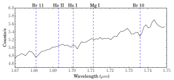
Figure 13: The UKIRT-UIST spectrum extracted over a 6 pixel wide aperture centered on the radio component, R1 is shown here. The spectral range is chosen to be the same as the VLT-ISAAC spectrum towards the infrared source, IRAS 18079-1756, associated with G12.42+0.50, studied by Kendall, de Wit & Yun (2003). The absorption lines identified by these authors are indicated in the plot.

From the Lyman continuum photon flux and the electron density estimates, we compute the radius of the Strömgren sphere, that is defined as the radius at which the rate of ionization equals the rate of recombination, assuming that the H ii region is expanding in a homogeneous and spherically, symmetric medium. The radius of the Strömgren sphere, $R_{s}$ is given by the expression,

$$R_{s}=\bigg{(}\frac{3N_{Ly}}{4\pi n_{0}^{2}\alpha_{B}}\bigg{)}^{1/3}$$ (12)

where $\alpha_{B}$ is the radiative recombination coefficient taken to be $\rm 2.6\times 10^{-13}~{}cm^{3}~{}s^{-1}$ (Kwan, 1997) and $n_{0}$ is the mean number density of atomic hydrogen which is estimated to be $\rm 2.1\times 10^{4}~{}cm^{-3}$ from the clump detected in the column density map (Section 3.3.3). Thus, the radius of the Strömgren sphere, $R_{s}$ for the resolved component, R1 is calculated to be 0.007 pc. Using this, the dynamical age the H ii region is determined from the expression

$$t_{dyn}=\bigg{[}\frac{4\,R_{s}}{7\,c_{i}}\bigg{]}\bigg{[}\bigg{(}\frac{R_{\mbox{H\,{\sc ii}}}}{R_{s}}\bigg{)}^{7/4}-1\bigg{]}$$ (13)

where $R_{\mbox{H\,{\sc ii}}}$, is the radius of the H ii region, $c_{i}$ is the isothermal sound speed in the ionized medium, which is typically assumed to be $\rm 10~{}km~{}s^{-1}$. $R_{\mbox{H\,{\sc ii}}}$ is estimated to be 0.01 pc by taking the geometric mean of the deconvolved size given in Table 4. The dynamical age of the UC H ii region associated with component R1 is determined to be $0.4\times 10^{3}$ yr. Since this estimation is made under a not so realistic assumption that the medium in which the H ii region expands is homogeneous, the results obtained may be considered representative at best. The derived physical parameters of the UC H ii region are tabulated in Table  12. The estimated values of electron density and emission measure are in the range found for UC H ii regions around stars of spectral type $\rm B1-B0.5$ (Kurtz, Churchwell & Wood, 1994). Furthermore, the size estimates for UC H ii regions are proposed to be $\rm\lesssim 0.1~{}pc$ (Wood & Churchwell, 1989; Kurtz, 2002), in agreement with that derived for the component R1. The dynamical timescales obtained indicate a very early phase of the UC H ii region (Wood & Churchwell, 1989; Churchwell, 2002). Wood & Churchwell (1989) estimate that it would take $\sim 10^{4}$ yr for an UC H ii region to expand against the gravitational pressure of the confining dense molecular cloud.

On a careful scrutiny of the point sources in the region, it is seen that a red 2MASS source (J18105109-1755496; $J$ = 13.727, $H$ = 11.011, $K$ = 9.351) is located at the peak position of R1 (within $\sim 0.3^{\prime\prime}$). Investigating its location in $JHK$ colour-colour diagrams (e.g Fig.  6(d) of Das et al. (2017)) suggests a highly embedded Class II YSO which in all likelihood could be the ionizing source. Detailed spectroscopic observations of this source is presented in Kendall, de Wit & Yun (2003). In the observed wavelength range of $1.67-1.75$ $\rm\mu m$, the VLT/ISAAC $H$-band spectra, presented by these authors, show the presence of broad absorption features of He I ($\sim$ 1.7 $\rm\mu m$) and hydrogen. We did a careful examination of our UKIRT spectroscopic observations. We extracted the spectrum over a 6 pixel wide aperture (estimated from other stellar sources along the slit) centred on R1, a zoom in of which is shown in Fig. 13. The spectral range is chosen such that it matches the VLT spectrum of Kendall, de Wit & Yun (2003) (refer Fig. 5 of their paper). Inspite of the poor signal-to-noise, the spectrum does show hint of the Br 11 line and possibly the Br 10 line as well as detected by Kendall, de Wit & Yun (2003). Based on these absorption lines and the absence of the 1.693 $\rm\mu m$ He II absorption line, Kendall, de Wit & Yun (2003) suggest this source to be a main-sequence star of spectral type B3 ($\pm 3$ subclasses). This is consistent with the spectral type derived from our measured radio flux densities. However, the absence of emission lines in their observed spectra prompted the authors to speculate a late evolutionary stage. This contradicts the results obtained from our $HK$ and $KL$ spectra which show the presence of several emission lines that are listed in Table 5, indicating an early evolutionary phase. The results from the molecular line analysis discussed in Section 4.2 is also in agreement with this picture. The compact component R2 can either be an independent UC H ii region or an externally ionized density clump. If we consider it as an UC H ii region then the observed Lyman continuum flux translates to an ionizing source of spectral type $\rm B3-B2$ (Panagia, 1973) and a mass of $6-9$ M_⊙(Davies et al., 2011).

4.1.2 A possible thermal jet?

Even with the compelling possibility of R1 being an UC H ii region, we explore an alternate scenario along the lines of a possible thermal jet. This is motivated by the very nature of G12.42+0.50 which is identified as an EGO and hence likely to be associated with jets/outflows. Further, several observational manifestations are consistent with the characteristics of thermal radio jets listed in Anglada (1996) and Rodriguez (1997).

G12.42+0.50 is a weak radio source (integrated flux density $<$ 10 mJy) displaying a linear morphology, including components R1 and R2, in the north-east and south-west direction. It is also seen to be associated with a large scale molecular outflow (Fig. 15(a), Section 4.2.2) with the candidate jet located at its centroid position and the observed elongation aligned with the outflow axis. From the radio spectral index map shown in Fig. 3, we see that along the direction of the radio components R1 and R2, the spectral index varies between $\sim 0.3-0.7$. These values of spectral index are consistent with the radio continuum emission originating due to the thermal free-free emission from an ionized collimated stellar wind (Panagia & Felli, 1975; Reynolds, 1986; Anglada et al., 1998). Similar range of spectral index values are also cited in literature for systems harbouring thermal radio jets (Anglada et al., 1994; Guzmán, Garay & Brooks, 2010; Sanna et al., 2016). Additional support for the thermal jet hypothesis comes from the angular size spectrum. Guzmán et al. (2016) and Hofner et al. (2017) have discussed the trend of the angular size spectrum where the jet features show a decrease in size with frequency as expected from the variation of electron density with frequency (Panagia & Felli, 1975; Reynolds, 1986). In case of G12.42+0.50, the 1390 MHz and 5 GHz sizes show this trend with the upper limit from 610 MHz being consistent. It should be noted here that in the 5 GHz map, all structures upto $\sim 20\arcsec$ would be well-imaged (Urquhart et al., 2009). However, the size dependence is not conclusive given the resolution of the two maps. Presence of shock-excited emission lines in the NIR (Section 3.2) further corroborates with this ionized jet scenario. Additionally, a $\rm H_{2}O$ maser is seen to be associated with G12.42+0.50 (Cyganowski et al., 2013), located at an angular distance of $\sim$12$\arcsec$ from the radio peak. The position of this is indicated in Fig. 1(b) and (c) and Fig. 15(b). $\rm H_{2}O$ masers have often been found in the vicinity of thermal radio jets, and in some cases both the thermal jet and $\rm H_{2}O$ masers are powered by the same star (Gomez, Rodriguez & Marti, 1995).

The two competing schemes deliberated above are in good agreement with our observation making it difficult to be biased towards any. However, recent studies speculate about the co-existence of UC/HC H ii regions and ionized jets. From the investigation of the nature of the observed centimetre radio emission in G35.20-0.74N, Beltrán et al. (2016) discuss the possibility of it being a UC H ii region as well as a radio jet being powered by the same YSO suggesting an interesting transitional phase where the UC H ii region has started to form while infall and outflow processes of the main accretion phase is still ongoing. Similar scenario is also invoked for the MYSO, G345.4938+01.4677 by Guzmán et al. (2016). Both these examples conform well with our results. Guzmán, Garay & Brooks (2010) discuss about a string of radio sources which are likely to be the ionized emission due to shocks from fast jets wherein the separation of the inner lobe from the central object is $\sim 0.03$ pc. Garay et al. (2003) also examines a radio triple source in which case the central source harbours a high-mass star in an early evolutionary phase and ejects collimated stellar wind which ionizes the surrounding medium giving rise to the observed radio emission. In this case, the separation between the central source and the radio lobe is $\sim$ 0.14 pc. For G12.42+0.50, component R2, at a distance of $\sim 0.07$ pc from R1, can also be conjectured to be a clumpy, enhanced density region (SMA3) ionized by the emanating jet. The star forming region of G12.42+0.50 has also been speculated to be harbouring a cluster (Jaffe et al., 1984; Kendall, de Wit & Yun, 2003). With the detection of R1, R2, SMA1 and SMA2, it reveals itself as a potentially active star forming complex.

4.2 Kinematic Signatures of gas motion

4.2.1 Infall activity

Table 13: The infall velocity, $V_{\rm inf}$ and mass infall rate, $\dot{M}_{\rm inf}$ of the clump, C1 associated with G12.42+0.50, estimated using the blue-skewed optically thick $\rm HCO^{+}$ line

$V_{\rm LSR}$	$V_{\rm inf}$	$\delta V$	$\dot{M}_{\rm inf}$
($\rm km~{}s^{-1}$)	($\rm km~{}s^{-1}$)		($10^{-3}$ M⊙yr-1)
18.3	1.8	-0.6	9.9

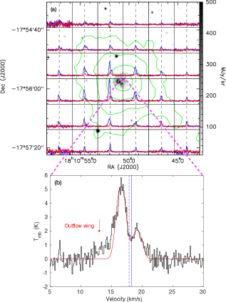
Figure 14: (a) The grey scale shows the 4.5 $\rm\mu m$ map. The green contours represent the ATLASGAL 870 $\rm\mu m$ emission. The contour levels are 3, 9, 27, 72 and 108 times $\sigma$ ($\sigma\sim 0.06$ Jy/beam). The $\rm HCO^{+}$ spectrum shown in blue and the $\rm H^{13}CO^{+}$ spectrum shown in red are overlaid. The spectra are boxcar-smoothed by five channels that corresponds to a velocity smoothing of $\rm 0.6~{}km~{}s^{-1}$. The dashed vertical lines indicate the LSR velocity estimated by averaging the peak positions of the $\rm H^{13}CO^{+}$ line in all the regions where the line is detected. The peak position of the 870 $\rm\mu m$ emission is marked by a magenta ‘x’. (b) The $\rm HCO^{+}$ spectrum extracted towards the ATLASGAL 870 $\rm\mu m$ peak . The best fit obtained using the ‘two-layer’ model is shown in red. The solid blue line represents the LSR velocity, $\rm 18.3~{}km~{}s^{-1}$ derived from the optically thin $\rm H^{13}CO^{+}$ line and the dashed blue line represents the LSR velocity obtained from the model fit. The red arrow points to a blue-wing which could indicate a possible molecular outflow.

Table 14: Best fit parameters retrieved from the model for the self-absorbed $\rm HCO^{+}$ line observed towards G12.42+0.50.

$\tau_{0}$	$\Phi$	$J_{c}$	$J_{f}$	$J_{r}$	$V_{\rm cont}$	$\sigma$	$V_{\rm rel}$
		(K)	(K)	(K)	($\rm km~{}s^{-1}$)	($\rm km~{}s^{-1}$)	($\rm km~{}s^{-1}$)
1.3	0.3	13.9	7.4	10.6	17.9	0.7	1.3

The double-peaked, blue-asymmetric $\rm HCO^{+}$ line profile with a self-absorption dip shown in Fig. 11 is a characteristic signature of infall activity (De Vries & Myers, 2005; Peretto, André & Belloche, 2006; Peretto et al., 2013; Yuan et al., 2018). In order to probe the gas motion in the entire clump associated with G12.42+0.50, we generate a grid map of the $\rm HCO^{+}$ line profile which is presented in Fig. 14(a). $\rm HCO^{+}$ line profiles are displayed in blue. For comparison, we also plot the optically thin transition, $\rm H^{13}CO^{+}$, in red. The grey scale map shows the 4.5 $\rm\mu m$ map emission with the ATLASGAL contours (in green) overlaid. The spectra shown here are averaged over regions gridded to an area given by the square of the beam size (36$\arcsec$) of the Mopra radio telescope. The $\rm HCO^{+}$ spectrum displays blue-skewed line profiles in all the grids within ATLASGAL contour revealing a strong indication of the clump in global collapse. For the molecular cloud to be collapsing, the gravitational energy of the cloud has to overcome the kinetic energy that supports it from collapsing. The gravitational stability of the cloud can be inspected using the virial parameter, $\alpha_{\rm vir}=5\sigma^{2}R/(GM_{\rm C})$ which needs to be lower than unity (Bertoldi & McKee, 1992) for a collapsing cloud. $\sigma$ is the velocity dispersion which is taken from the FWHM of the optically thin $\rm H^{13}CO^{+}$ line and is estimated to be $\rm 1.2~{}km~{}s^{-1}$. Taking $R$ and $M_{\rm C}$ as the radius and mass of the clump, C1, the virial parameter, $\alpha_{\rm vir}$ is calculated to be $\sim 0.9$. In comparison, Yuan et al. (2018) obtain a value of 0.58 for the EGO G022.04+0.22 and Pillai et al. (2011) in their study of massive cores obtain values in the range $0.1-0.8$. Given the presence of infall and outflow activity, that could significantly increase the velocity dispersion, the derived estimate towards G12.42+0.50 is likely to be an overestimate.

To support the picture of protostellar infall, we estimate the infall velocity and mass infall rate. First, to quantify the blue-skewness of the $\rm HCO^{+}$ profile, we calculate the asymmetry parameter, $\delta V$, using the following expression (Yu & Wang, 2013),

$$\delta V=\frac{(V_{\rm thick}-V_{\rm thin})}{\Delta V_{\rm thin}}$$ (14)

Here, $\delta V$ is defined as the ratio of the difference between the peak velocities of the optically thick line, $V_{\rm thick}$ and the optically thin line, $V_{\rm thin}$, and the FWHM of the optically thin line denoted by $\Delta V_{\rm thin}$. Using values of $V_{\rm thin}=18.3{\rm~{}km~{}s^{-1}}$ and $\Delta V_{\rm thin}=2.9{\rm~{}km~{}s^{-1}}$ from the Gaussian fit to the $\rm H^{13}CO^{+}$ line and $V_{\rm thick}=16.5{\rm~{}km~{}s^{-1}}$, the peak of the blue component of the $\rm HCO^{+}$ line, $\delta V$ is estimated to be $-0.6$. According to Mardones et al. (1997), the criteria for a bona fide blue-skewed profile is $\delta V<-0.25$. Furthermore, we estimate the mass infall rate ($\dot{M}_{\rm inf}$) of the envelope using the equation, $\dot{M}_{\rm inf}=4\pi R^{2}V_{\rm inf}\rho$ (López-Sepulcre, Cesaroni & Walmsley, 2010), where $V_{\rm inf}$ = $V_{\rm thin}-V_{\rm thick}$ = $V_{\rm H^{13}{CO}^{+}}-V_{\rm HCO^{+}}$ is the infall velocity and $\rho$ is the average volume density of the clump given by $\rho=M_{\rm C}/\frac{4}{3}\pi R^{3}$. The clump mass, $M_{\rm C}$ and radius, $R$ are taken from Section 3.3.4. The infall velocity, $V_{\rm inf}$ and the mass infall rate are estimated to be $\rm 1.8~{}km~{}s^{-1}$ and $\rm 9.9\times 10^{-3}$ M_⊙yr^-1, respectively. The mass infall rate estimate is higher compared to the value of $6.4\times 10^{-3}$ M_⊙yr^-1 derived by He et al. (2015). As discussed in Section 3.3.4, our clump mass and radius estimates are higher. Nevertheless, both the estimates fall in the range seen in other high mass star forming regions (Chen et al., 2010; López-Sepulcre, Cesaroni & Walmsley, 2010; Liu et al., 2013).

To further understand the properties of the infalling gas, we extend our analysis and fit the $\rm HCO^{+}$ line with a ‘two-layer’ model following the discussion in Liu et al. (2013). Here, we briefly repeat the salient features of the model with a description of the equations and the terms. In this model, a continuum source is located in between the two layers, with each layer having an optical depth, $\tau_{0}$ and velocity dispersion, $\sigma$, and an expanding speed, $V_{\rm rel}$ with respect to the continuum source. This is the infall velocity introduced earlier. $V_{\rm rel}$ is negative if the gas is moving away and positive when there is inward motion. The brightness temperature at velocity, $V$ is given by

$$\Delta T_{B}=(J_{f}-J_{cr})[1-exp(-\tau_{f})]\\ +(1-\Phi)(J_{r}-J_{b})\times[1-exp(-\tau_{r}-\tau_{f})]$$ (15)

where

$$J_{cr}=\Phi J_{c}+(1-\Phi)J_{r}$$ (16)

and

$$\tau_{f}=\tau_{0}exp\bigg{[}\frac{-(V-V_{\rm rel}-V_{\rm cont})^{2}}{2\sigma^{2}}\bigg{]}$$ (17)

$$\tau_{r}=\tau_{0}exp\bigg{[}\frac{-(V+V_{\rm rel}-V_{\rm cont})^{2}}{2\sigma^{2}}\bigg{]}$$ (18)

Here $J_{c}$, $J_{f}$, $J_{r}$, $J_{b}$ are the Planck temperatures of the continuum source, the “front” layer, the “rear” layer and the cosmic background radiation, respectively. $J$ is the blackbody function at temperature, $T$ and frequency, $\nu$ and is expressed as

$$J=\frac{h\nu}{k}\frac{1}{exp(T_{0}/T)-1}$$ (19)

where $T_{0}=h\nu/k$, $h$ is Planck’s constant, and $k$ is Boltzmann’s constant. $\Phi$ and $V_{\rm cont}$ are the filling factor and systemic velocity (or the LSR velocity) of the continuum source, respectively. The $\rm HCO^{+}$ profile and the fitted spectrum (in red) are displayed in Fig. 14(b). The LSR velocities determined from the model fit (dashed blue) and the optically thin transition of $\rm H^{13}CO^{+}$ (solid blue) are also shown in the figure. The blue component of the $\rm HCO^{+}$ line shows a clear presence of broadened wing likely to be due to outflow. To avoid contamination from this outflow component, we restrict the velocity range between $\rm 16.1-21.0~{}km~{}s^{-1}$ while fitting the model. The model derived parameters are listed in Table 14. The model fitted values are fairly consistent (slightly smaller) with our previous estimates.

4.2.2 Outflow feature

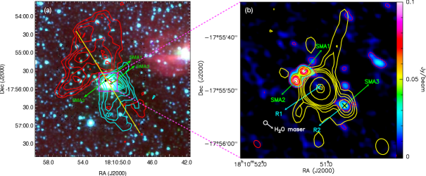
Figure 15: (a) The Spitzer IRAC colour composite image of G12.42+0.50, overlaid with the SMA 1.1 mm emission contours in black, with the contour levels same as in Fig. 7(k). The $\rm{}^{12}CO~{}(3-2)$ emission integrated from the peak of the blueshifted profile to the blue wings ($\rm 9.3-15.8~{}km~{}s^{-1}$) is represented using blue contours and from the peak of the red profile to the red wings ($\rm 20.8-27.3~{}km~{}s^{-1}$) is represented using red contours. The contours start from the $5~{}\sigma$ level for both the red and blue lobes and increases in steps of $3~{}\sigma$ and $4~{}\sigma$, respectively ($\rm\sigma=2.7~{}K~{}km~{}s^{-1}$ for red lobe and $\rm\sigma=2.3~{}K~{}km~{}s^{-1}$ for blue lobe ). The yellow line defines the cut along which the position-velocity (PV) diagram is made. The cut is selected in such a way that it passes through the red and blue lobes and also through the extended green emission. The red and blue lobes of the molecular outflow lie along a similar axis as the ionized jet. (b) The colour scale represents the 1.1 mm continuum emission from SMA observed towards G12.42+0.50 with the contour levels same as in Fig. 8(k). Radio emission at 1390 MHz is represented by yellow contours with the contour levels same as that in Fig. 2(a). The restoring beams of the 1390 MHz map and 1.1 mm map are indicated at the bottom- right and left of the image, respectively. The ‘x’s indicate the positions of R1 and R2. The white circle marks the position of the $\rm H_{2}O$ maser in the vicinity of G12.42+0.50.

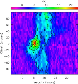
Figure 16: The PV diagram of the $\rm{}^{12}CO~{}(3-2)$ transition along the cut shown in yellow in Fig. 15(a) at a position angle of 32^∘. The contour levels are 4, 9, 14 and 18 times $\sigma$ ($\sigma\sim 1.0~{}\rm K$). The zero offset in the PV diagram corresponds to the position of the central coordinate of G12.42+0.50 ($\rm\alpha_{J2000}=18^{h}10^{m}51.1^{s},\delta_{J2000}=-17\degree 55\arcmin 50\arcsec$). The LSR velocity, $\rm 18.3~{}km~{}s^{-1}$, is represented by the dashed red line.

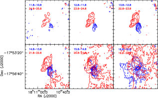
Figure 17: Channel maps of $\rm{}^{12}CO~{}(3-2)$ line associated with molecular cloud harbouring G12.42+0.50. Each box contains a pair of maps corresponding to the red- and blueshifted emission at the same offset from the LSR velocity. The channel widths are indicated at the top left of each map. The red contours correspond to the red wing and the blue contours correspond to the blue wing. The contours start from the 3$\sigma$ level of each map and increases in steps of 3$\sigma$.

Massive molecular outflows are ubiquitous in star forming regions (Beuther et al., 2002b) and often co-exist with ionized jets (e.g. Anglada, 1996; Purser et al., 2016). The jets are believed to entrain the gas and dust from the ambient molecular cloud, thus driving molecular outflows. According to several studies, broad wings of the optically thick lines like $\rm HCO^{+}$ are well accepted signatures of outflow activity (e.g. Klaassen & Wilson, 2007; Schneider et al., 2010; Smith et al., 2013). As mentioned in the previous section, broadening of the blue wing of the infall tracer line of $\rm HCO^{+}$ is seen in G12.42+0.50. Given the association with an EGO and the alignment with a large scale CO outflow features, the origin of the broad blue wing can be attributed to be due to the outflow. Alternate scenarios like unresolved velocity gradients (Tackenberg et al., 2014) or gravo-turbulent fragmentation (Klessen et al., 2005) have been invoked for broadened wings but are less likely to be the case here. In this section, we focus on the rotational transition lines of CO that are well known tracers of molecular outflow, and investigate the outflow kinematics of the molecular cloud associated with G12.42+0.50 using the archival data of the isotopologues of $\rm CO~{}(3-2)$ transition from JCMT and $\rm{}^{13}CO~{}(1-0)$ observation from TRAO.

The red and blueshifted velocity profiles of the CO transitions shown in Fig. 12(a) can be attributed to emission arising from distinct components of the CO gas that are moving in opposite directions away from the central core. We note that the peaks have different shifts with respect to the LSR velocity with the $\rm{}^{12}CO~{}(3-2)$ line showing the maximum shift and $\rm C^{18}O~{}(3-2)$ line has the minimum shift. The peaks of the red component of $\rm{}^{12}CO~{}(3-2)$, $\rm{}^{13}CO~{}(3-2)$ and $\rm C^{18}O~{}(3-2)$ transitions are shifted by 2.5, 1.6 and $\rm 1.0~{}km~{}s^{-1}$ from the LSR velocity. For the blue component the shifts are 2.5, 1.7 and $\rm 0.9~{}km~{}s^{-1}$, respectively. $\rm{}^{12}CO$ molecule, having the lowest critical density among the three, effectively traces the outer envelope of the molecular cloud, hence showing the maximum shift and the $\rm C^{18}O$ molecule, the densest among the three species is a tracer of the dense core of the molecular cloud and thus shows the minimum shift.

In order to map the outflow in the vicinity of G12.42+0.50, we construct the zeroth moment map of the two components using the task, IMMOMENTS in CASA. The zeroth moment map is the integrated intensity map that gives the intensity distribution of a molecular species within the specified velocity range. The $\rm{}^{12}CO~{}(3-2)$ emission is integrated from the peak of the blueshifted profile to the blue wings that corresponds to the lower velocity channels ranging from $\rm 9.3-15.8~{}km~{}s^{-1}$ for the blue component and from the peak of the redshifted profile to the red wing that corresponds to the higher velocity channels ranging from $\rm 20.8-25.3~{}km~{}s^{-1}$ for the red component. The contours are shown overlaid on the Spitzer IRAC colour composite image in Fig. 15(a). The figure reveals the presence of two distinct, spatially separated red and blue lobes. High-velocity gas is also seen towards the tail of the blue component. The location of the 1.1 mm dense cores, SMA1, SMA2 and SMA3 are also marked in this figure. The central part covering the brightest portion of the IRAC emission (location of the EGO), is shown in Fig. 15(b) with the spatial distribution of the ionized gas overlaid on the 1.1 mm dust emission. To corroborate with the zeroth moment map showing the outflow lobes, in Fig. 16, we show the position-velocity (PV) diagram constructed along the outflow direction (position angle of $\rm\sim 32^{\circ}$; east of north) highlighted in Fig. 15(a). The direction along which the PV diagram is made is chosen such that both the red and blue lobes are sampled and it also covers the region of extended 4.5 $\rm\mu m$ emission of G12.42+0.50. The zero offset in the PV diagram corresponds to the position of the central coordinate of the EGO, G12.42+0.50 ($\rm\alpha_{J2000}=18^{h}10^{m}51.1^{s},\delta_{J2000}=-17\degree 55\arcmin 50\arcsec$). As expected, the PV diagram also clearly reveals distinct red and blue components of the $\rm{}^{12}CO~{}(3-2)$ emission from the LSR velocity of the cloud represented by a red dashed line. Towards the lower region of the PV diagram we can trace a weaker redshifted $\rm{}^{12}CO~{}(3-2)$ component consistent with the high-velocity tail seen in the zeroth moment map.

To further probe the velocity structure of the cloud associated with G12.42+0.50, we generate channel maps of the $\rm{}^{12}CO~{}(3-2)$ emission following the method outlined in Sanna et al. (2014). To define suitable velocity ranges and identify the blue and redshifted outflow emission, we set the inner limits of the velocity at $\sim V_{\rm LSR}\pm{\rm FWHM}/2$, where FWHM is the $\rm H^{13}CO^{+}$ linewidth. Taking the offset to be $\rm\pm 1.5~{}km~{}s^{-1}$ from the LSR velocity, the inner velocity limit for the red and the blueshifted lobes are estimated to be $\rm 19.8~{}km~{}s^{-1}$ and $\rm 16.8~{}km~{}s^{-1}$, respectively. The channel maps constructed are shown in Fig. 17. Each grid displays a pair of maps with a velocity width of $\rm 1~{}km~{}s^{-1}$. Prominent outflow features begin to appear at velocities $\rm\sim 13.8$ and $\rm 21.8~{}km~{}s^{-1}$ from the blue and red components, respectively. Beyond these velocities there is no contribution from the central core. Closer to the LSR velocity, the emission is rather complex making it difficult for the outflow features to be discernible. This is understandable since near the LSR velocity, the emission from the outflow components is likely to be contaminated by the infall motion and contribution from the diffuse gas. The channel maps are comparable to those presented by Qiu et al. (2009) for the region G240.31+0.07 with similar complex velocity structure near the LSR. The channel maps also show the presence of a redshifted component between velocities $\rm 20.8-22.8~{}km~{}s^{-1}$ overlaping with the blue lobe towards the south-west. As will be discussed later in Section 4.2.3, such a velocity distribution can be indicative of accretion through filaments.

Morphologically, the spatially separated red and blue lobes associated with G12.42+0.50 resembles a wide-angle bipolar outflow seen in the star forming region G240.31+0.07 studied by Qiu et al. (2009). These authors suggest the wide-angle bipolar outflow as the ambient gas being swept up by an underlying wide-angle wind and is driven by one of the three mm peaks located close to the geometric centre of the bipolar outflow. Only a handful of studies have found the presence of wide-angle bipolar molecular outflows associated with high mass star formation (e.g. Shepherd et al., 1998; Qiu et al., 2009). Shepherd et al. (1998) investigate the likely driving source of the poorly collimated molecular outflow associated with G192.16. Coexistence of wide-angle CO outflow with shock-excited H₂ emission, prompted them to conclude that the G192.16 outflow is powered by the combination of a disk-wind and a jet. Given the likely association of G12.42+0.50 with an ionized jet supported by the presence of shock-excited NIR H₂ lines, we propose a similar picture of coexistence of disk-wind and a jet, where the wide-angle bipolar CO outflow is likely to be driven by the underlying wide-angle wind.

Of crucial importance is the identification of the driving source for this outflow. Marseille et al. (2008) elucidates about the star forming region IRAS 18151-1208, where two detected bipolar outflows are shown to be powered by two mm sources, MM1 and MM2. They have also detected a third mm core, MM3 that does not show any outflow activity. Beuther et al. (2002b), in their statistical study of massive molecular outflows, state that a large fraction of their sample show bipolar outflow and these are seen to be associated with massive mm sources and in most cases, are centred on the mm peaks. As seen in Fig. 15, two mm cores (SMA1 and SMA2) are located towards the centroid of the bipolar outflow associated with G12.42+0.50. These are shown to be potential high-mass star forming cores, Further, the absence of radio emission and IR sources imply a very early evolutionary phase. We further investigate whether SMA1 and/or SMA2 are the powering sources of the CO bipolar outflow in G12.42+0.50.

Following Qiu et al. (2009), the dynamical timescale of the outflow seen associated with G12.42+0.50 is computed using the expression, $T_{dyn}=L_{flow}/v_{max}$, where $L_{flow}\sim 1.2~{}\rm pc$ is the half length of the end-to-end extension of the flow and $v_{max}\sim 9.0~{}\rm km~{}s^{-1}$ is the maximum flow velocity from the LSR velocity of the cloud. This yields a dynamical timescale of the outflow that is $\rm 1.3\times 10^{5}$ yr. Comparing with the results obtained by Qiu et al. (2009), Shepherd et al. (1998) and Shepherd, Testi & Stark (2003), our estimated value is in agreement with massive molecular outflow from an UC H ii region. This result supports our unfolding picture of radio component R1, where coexistence of an UC H ii region and an ionized thermal jet is seen and the large-scale CO outflow can also be attributed to the UC H ii region. However, it should also be kept in mind that unlike Qiu et al. (2009), there is no SMA core coinciding with R1. Moreover, their results are based on interferometric observations, whereas, the JCMT CO outflow data used here are from single-dish measurements. In these single-dish observations, the inner outflow jets are mostly unresolved and the measurements are less sensitive to high-velocity outflow emission resulting in an overestimation of the dynamical ages. Hence, one cannot rule out the possibility of SMA1 and/or SMA2 being the outflow driving sources similar to the case of AFGL 5142 (Liu et al., 2016b). If indeed the binary cores, SMA1 and SMA2 are the outflow driving cores, then the nature of the radio emission in R1 (and R2) can be thought of as ionized jet emission driven by the mm cores which also drives the large scale CO outflows detected. Possibility of multiple outflows from the mm cores and the UC H ii region also exists (Beuther et al., 2002a; Beuther, Schilke & Stanke, 2003). This advocates for high-resolution observations for a better understanding.

4.2.3 Hub-filament system

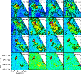
Figure 18: Channel maps of $\rm{}^{12}CO$ emission is shown here with each channel having a velocity width of $\rm 0.5~{}km~{}s^{-1}$. For each map, the black contours represent the $\rm{}^{12}CO$ emission starting from the $3\sigma$ level and increasing with a step of $3\sigma$.

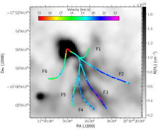
Figure 19: The velocity peaks of $\rm{}^{12}CO~{}(3-2)$ extracted along the filaments is overlaid on the column density map of the region associated with G12.42+0.50 shown in grey scale. The positions of all the filaments are also labelled.

From the above discussion we hypothesize a picture of global collapse of the molecular cloud harbouring the EGO, G12.42+0.50. Interestingly, Fig. 7(d) and (h), unfold the presence of large scale filamentary structures along the south-west direction of G12.42+0.50, all merging at the location of the clump, C1 enveloping G12.42+0.50. As mentioned earlier, the concurrence of a collapsing cloud with converging filaments suggest a hub-filament system. In literature, hub-filament systems are common in sites of high-mass star formation (e.g. Peretto et al., 2013; Liu et al., 2016b; Yuan et al., 2018). In such systems, converging flows are detected where matter funnels in through the filaments into the hub, where accretion is most pronounced. Morphologically, the molecular cloud system associated with G12.42+0.50 resembles the hub-filament system associated with the star forming region, G22 (Yuan et al., 2018) and the IRDC, SDC335 ($\rm SDC335.579-0.292$) (Peretto et al., 2013).

To delve deeper into this picture, we investigate the velocity structure of the filaments. To proceed, we construct the channel maps of the $\rm{}^{12}CO$ emission which are illustrated in Fig. 18. The velocity ranges are selected by examining the JCMT $\rm{}^{12}CO$ data cube and choosing the range where the $\rm{}^{12}CO$ emission is detected. The velocity width of each channel is chosen to be $\rm 0.5~{}km~{}s^{-1}$ similar to that used by Leurini et al. (2019) to investigate the $\rm C^{18}O~{}(2-1)$ emission associated with IRDC, G351.776-0.527. The spatial coincidence of the $\rm{}^{12}CO$ emission with the filaments is remarkable. The gas associated with the filaments is consistently redshifted with respect to the LSR velocity of the clump, C1. The velocity of the cloud along the filaments peak in the velocity range of $\rm\sim 18-23~{}km~{}s^{-1}$. The variation in velocity suggests bulk gas motion along the filaments. From the channel maps we can see that the velocity of the molecular gas along the filament decreases as it approaches the central core, with the maximum velocity at the south-west end of the filament. It has to be noted here that the $\rm{}^{12}CO~{}(3-2)$ transition is also a tracer of molecular outflow and as shown in Section 4.2.2, G12.42+0.50 is also an outflow source. Hence, the decrease in velocity near the clump, C1 may be attributed to the interaction with the molecular outflow.

To further elaborate on the velocity structure, we extract the spectra of $\rm{}^{12}CO~{}(3-2)$ along the filaments with a step size of half the angular resolution ($\sim 15^{\prime\prime}/2$) of the JCMT-HARP observation. The peak velocities estimated by fitting 1D Gaussian profiles to the spectra are shown in Fig. 19 as colour-coded circles overlaid on the H₂ column density map. Along the filaments, F1 and F6 it can be seen that the velocity is within the range $\rm 17-19~{}km~{}s^{-1}$, closer to the LSR velocity, and increasing towards the clump, C1. However, along the filaments F2, F3, and F4 the velocity is on the higher side of the LSR velocity, ranging from $\rm 19-21~{}km~{}s^{-1}$ and decreasing towards the central clump, C1. But in the case of filament, F5, we do not clearly notice any velocity gradient, and the values are seen to vary in the range $\rm 19-20~{}km~{}s^{-1}$. Similar velocity gradients along filaments are detected in star forming regions such as SDC335 (Peretto et al., 2013), G22 (Yuan et al., 2018) and AFGL 5142 (Liu et al., 2016b). Following these authors, we also attribute the velocity gradients to be due to gas inflow through filaments. A number of other mechanisms have also been proposed, which include filamentary collapse, filament collision, rotation, expansion and wind-acceleration to explain the observed velocity distributions (Peretto et al., 2014). If the velocity distribution were to be explained by expansion scenario, we should have observed red-skewed velocity profiles of optically thick lines ($\rm HCO^{+}$, HCN and HNC) towards the clump, C1 (Liu et al., 2018). On the contrary, we observe blue-skewed velocity profiles, hence rendering the expansion picture to be unlikely. Further, we do not observe any cloud collision signature of enhanced line-widths at the junction (Yuan et al., 2018). The molecular outflow likely to be driven by the thermal jet in the clump, C1, cannot possibly explain the red-skewed velocity along the filaments, $\rm F2-F5$, since these fall along the blue lobe of the detected outflow. Also, in general, outflows are located between filaments (Liu et al., 2016b). Hence, on comparison with earlier studies and the lack of evidence to prove otherwise, we infer that the observed velocity gradient is a result of gas inflow along the filaments, although there could be contribution from the outflowing gas. Nonetheless, $\rm{}^{12}CO~{}(3-2)$ being an optically thick molecular line transition, cannot effectively probe the velocity distribution within the filaments. Thus, high resolution observations of optically thin lines would give a better picture. As discussed in Section 3.3.4, 11 eleven clumps, $\rm C2-C12$, lie along the identified filaments. It is also seen that along the filaments the dust temperature is lower than C1. The mass estimates show that these are less massive than the central core (clump, C1). Yuan et al. (2018), in the study of the hub-filament system associated with G22, finds two clumps more massive than the other clumps along the filament. These clumps,that dominate the emission at wavelengths longer than 24 $\rm\mu m$ are the most active star forming regions in G22. This concurs well with G12.42+0.50, where the most massive clump, C1, is an active star forming clump.

5 SUMMARY

We carried out a comprehensive multiwavelength study towards the EGO, G12.42+0.50 and its associated environment. Our main results are summarized as follows

1. The radio continuum emission mapped at 1390 MHz reveals a linear structure extended in the north-east and south-west direction with the presence of two compact radio components, R1 and R2 that are unresolved at 610 MHz. The peak emission at 610 MHz is coincident with the component R1.

2. We explore different scenarios to explain the nature of the ionized emission. Under the UC H ii framework, assuming the emission at 1390 MHz to be optically thin, the observed Lyman continuum flux translates to an ionizing source of spectral type of $\rm B1-B0.5$. An alternative picture of ionized thermal jet is examined, given various observed characteristics including the spectral index values of $0.3-0.9$ in the region. We are prompted to consider the co-existence of the UC H ii region with an ionized jet being powered by the same YSO. IRAS 18079-1756 (2MASS J18105109-1755496), a deeply embedded Class II YSO is likely to be the driving source.

3. Presence of shock-excited H₂ and [FeII] line emission is confirmed from NIR narrow-band imaging and spectroscopy in concurrence with the jets/outflows picture.

4. A massive central clump, C1 is identified from the 870 $\rm\mu m$ map which envelopes the detected radio and the enhanced and extended 4.5 $\rm\mu m$ emission. The clump has a mass 1375 M_⊙ and total luminosity $\rm 2.8\times 10^{4}~{}L_{\odot}$. Two-component modeling shows the presence of an inner warm component surrounded by an extended outer, cold envelope traced mostly by the FIR wavelengths

5. Seven molecular species from the MALT90 survey are detected towards the EGO, G12.42+0.50. The optically thick lines, $\rm HCO^{+}$ and HCN show signatures of protostellar infall. From the blue-skewed profile of the $\rm HCO^{+}$ line, infall velocity and mass infall rate are estimated to be $\rm 1.8~{}km~{}s^{-1}$ and $\rm 9.9\times 10^{-3}~{}M_{\odot}yr^{-1}$.

6. From the line observations of the $J=3-2$ transition of the molecular species $\rm{}^{12}CO$, $\rm{}^{13}CO$ and $\rm C^{18}O$, we detect the presence of a wide-angle bipolar outflow. From the dynamical age, $\rm 1.3\times 10^{5}~{}yr$, of the bipolar outflow it seems likely that the UC H ii drives the same though the possibility of the SMA cores (SMA1 and SMA2) being the powering source(s) cannot be ruled out.

7. Signature of a hub-filament system is seen in the 8.0 $\rm\mu m$ and FIR images and is supported by the constructed column density and dust temperature maps. A detailed study of the gas kinematics agrees with bulk motion in the filaments and suggest a likely picture of gas inflow along the filaments to C1.

8. A conjectured hypothesis of the EGO, G12.42+0.50, satisfying the multiwavelength observations, could be an active star forming complex where very early evolutionary cores (SMA1 and SMA2) are seen. Apart from this, an accreting (likely through filaments) MYSO in an initial phase of an UC H ii region and driving a large-scale molecular outflow entrained by a likely ionized thermal jet is detected.

References

- Anderson et al. (2010) Anderson L. D. et al., 2010, \aap, 518, L99
- André et al. (2010) André P. et al., 2010, \aap, 518, L102
- Anglada (1996) Anglada G., 1996, in Astronomical Society of the Pacific Conference Series, Vol. 93, Radio Emission from the Stars and the Sun, Taylor A. R., Paredes J. M., eds., pp. 3–14
- Anglada et al. (1994) Anglada G., Rodriguez L. F., Girart J. M., Estalella R., Torrelles J. M., 1994, \apjl, 420, L91
- Anglada et al. (1998) Anglada G., Villuendas E., Estalella R., Beltrán M. T., Rodríguez L. F., Torrelles J. M., Curiel S., 1998, \aj, 116, 2953
- Aniano et al. (2011) Aniano G., Draine B. T., Gordon K. D., Sandstrom K., 2011, \pasp, 123, 1218
- Arthur et al. (2004) Arthur S. J., Kurtz S. E., Franco J., Albarrán M. Y., 2004, \apj, 608, 282
- Battersby et al. (2011) Battersby C. et al., 2011, \aap, 535, A128
- Beckwith et al. (1990) Beckwith S. V. W., Sargent A. I., Chini R. S., Guesten R., 1990, \aj, 99, 924
- Beltrán et al. (2016) Beltrán M. T., Cesaroni R., Moscadelli L., Sá nchez-Monge Á., Hirota T., Kumar M. S. N., 2016, \aap, 593, A49
- Benjamin et al. (2003) Benjamin R. A. et al., 2003, \pasp, 115, 953
- Bertoldi & McKee (1992) Bertoldi F., McKee C. F., 1992, \apj, 395, 140
- Beuther et al. (2002a) Beuther H., Schilke P., Gueth F., McCaughrean M., Andersen M., Sridharan T. K., Menten K. M., 2002a, \aap, 387, 931
- Beuther et al. (2002b) Beuther H., Schilke P., Sridharan T. K., Menten K. M., Walmsley C. M., Wyrowski F., 2002b, \aap, 383, 892
- Beuther, Schilke & Stanke (2003) Beuther H., Schilke P., Stanke T., 2003, \aap, 408, 601
- Buckle et al. (2009) Buckle J. V. et al., 2009, \mnras, 399, 1026
- Caratti o Garatti et al. (2015) Caratti o Garatti A., Stecklum B., Linz H., Garcia Lopez R., Sanna A., 2015, \aap, 573, A82
- Casali et al. (2007) Casali M. et al., 2007, \aap, 467, 777
- Chambers et al. (2009) Chambers E. T., Jackson J. M., Rathborne J. M., Simon R., 2009, \apjs, 181, 360
- Chen et al. (2011) Chen X., Ellingsen S. P., Shen Z.-Q., Titmarsh A., Gan C.-G., 2011, \apjs, 196, 9
- Chen et al. (2013) Chen X., Gan C.-G., Ellingsen S. P., He J.-H., Shen Z.-Q., Titmarsh A., 2013, \apjs, 206, 22
- Chen et al. (2010) Chen X., Shen Z.-Q., Li J.-J., Xu Y., He J.-H., 2010, \apj, 710, 150
- Churchwell (2002) Churchwell E., 2002, \araa, 40, 27
- Csengeri et al. (2016) Csengeri T. et al., 2016, \aap, 585, A104
- Curiel et al. (1993) Curiel S., Rodriguez L. F., Moran J. M., Canto J., 1993, \apj, 415, 191
- Currie et al. (2008) Currie M. J., Draper P. W., Berry D. S., Jenness T., Cavanagh B., Economou F., 2008, in Astronomical Society of the Pacific Conference Series, Vol. 394, Astronomical Data Analysis Software and Systems XVII, Argyle R. W., Bunclark P. S., Lewis J. R., eds., p. 650
- Cyganowski et al. (2009) Cyganowski C. J., Brogan C. L., Hunter T. R., Churchwell E., 2009, \apj, 702, 1615
- Cyganowski et al. (2011a) Cyganowski C. J., Brogan C. L., Hunter T. R., Churchwell E., 2011a, \apj, 743, 56
- Cyganowski et al. (2011b) Cyganowski C. J., Brogan C. L., Hunter T. R., Churchwell E., Zhang Q., 2011b, \apj, 729, 124
- Cyganowski et al. (2013) Cyganowski C. J., Koda J., Rosolowsky E., Towers S., Donovan Meyer J., Egusa F., Momose R., Robitaille T. P., 2013, \apj, 764, 61
- Cyganowski et al. (2008) Cyganowski C. J. et al., 2008, \aj, 136, 2391
- Das et al. (2017) Das S. R., Tej A., Vig S., Liu H.-L., Liu T., Ishwara Chandra C. H., Ghosh S. K., 2017, \mnras, 472, 4750
- Das et al. (2018) Das S. R., Tej A., Vig S., Liu T., Ghosh S. K., Chandra C. H. I., 2018, \aap, 612, A36
- Davies et al. (2011) Davies B., Hoare M. G., Lumsden S. L., Hosokawa T., Oudmaijer R. D., Urquhart J. S., Mottram J. C., Stead J., 2011, \mnras, 416, 972
- Davis et al. (2007) Davis C. J., Kumar M. S. N., Sandell G., Froebrich D., Smith M. D., Currie M. J., 2007, \mnras, 374, 29
- Davis et al. (2003) Davis C. J., Smith M. D., Stern L., Kerr T. H., Chiar J. E., 2003, \mnras, 344, 262
- De Buizer & Vacca (2010) De Buizer J. M., Vacca W. D., 2010, \aj, 140, 196
- De Vries & Myers (2005) De Vries C. H., Myers P. C., 2005, \apj, 620, 800
- Ellingsen (2006) Ellingsen S. P., 2006, \apj, 638, 241
- Fazio et al. (2004) Fazio G. G. et al., 2004, \apjs, 154, 10
- Foster et al. (2011) Foster J. B. et al., 2011, \apjs, 197, 25
- Froebrich et al. (2011) Froebrich D. et al., 2011, \mnras, 413, 480
- Garay et al. (2003) Garay G., Brooks K. J., Mardones D., Norris R. P., 2003, \apj, 587, 739
- Gomez, Rodriguez & Marti (1995) Gomez Y., Rodriguez L. F., Marti J., 1995, \apj, 453, 268
- Griffin et al. (2010) Griffin M. J. et al., 2010, \aap, 518, L3
- Guzmán, Garay & Brooks (2010) Guzmán A. E., Garay G., Brooks K. J., 2010, \apj, 725, 734
- Guzmán et al. (2016) Guzmán A. E., Garay G., Rodríguez L. F., Contreras Y., Dougados C., Cabrit S., 2016, \apj, 826, 208
- Haslam et al. (1982) Haslam C. G. T., Salter C. J., Stoffel H., Wilson W. E., 1982, \aaps, 47, 1
- He, Takahashi & Chen (2012) He J. H., Takahashi S., Chen X., 2012, \apjs, 202, 1
- He et al. (2015) He Y.-X. et al., 2015, \mnras, 450, 1926
- Hildebrand (1983) Hildebrand R. H., 1983, \qjras, 24, 267
- Hoare, Roche & Glencross (1991) Hoare M. G., Roche P. F., Glencross W. M., 1991, \mnras, 251, 584
- Hofner et al. (2017) Hofner P., Cesaroni R., Kurtz S., Rosero V., Anderson C., Furuya R. S., Araya E. D., Molinari S., 2017, \apj, 843, 99
- Inoue, Hirashita & Kamaya (2001) Inoue A. K., Hirashita H., Kamaya H., 2001, \apj, 555, 613
- Jackson et al. (2013) Jackson J. M. et al., 2013, \pasa, 30, e057
- Jaffe, Guesten & Downes (1981) Jaffe D. T., Guesten R., Downes D., 1981, \apj, 250, 621
- Jaffe et al. (1984) Jaffe D. T., Hildebrand R. H., Keene J., Harper D. A., Loewenstein R. F., Moran J. M., 1984, \apj, 281, 225
- Kauffmann et al. (2008) Kauffmann J., Bertoldi F., Bourke T. L., Evans, II N. J., Lee C. W., 2008, \aap, 487, 993
- Kauffmann et al. (2010a) Kauffmann J., Pillai T., Shetty R., Myers P. C., Goodman A. A., 2010a, \apj, 712, 1137
- Kauffmann et al. (2010b) Kauffmann J., Pillai T., Shetty R., Myers P. C., Goodman A. A., 2010b, \apj, 716, 433
- Kaufman et al. (1999) Kaufman M. J., Wolfire M. G., Hollenbach D. J., Luhman M. L., 1999, \apj, 527, 795
- Kendall, de Wit & Yun (2003) Kendall T. R., de Wit W. J., Yun J. L., 2003, \aap, 408, 313
- Klaassen & Wilson (2007) Klaassen P. D., Wilson C. D., 2007, \apj, 663, 1092
- Klessen et al. (2005) Klessen R. S., Ballesteros-Paredes J., Vázquez-Semadeni E., Durán-Rojas C., 2005, \apj, 620, 786
- Kobulnicky & Johnson (1999) Kobulnicky H. A., Johnson K. E., 1999, \apj, 527, 154
- Kurtz (2002) Kurtz S., 2002, in Astronomical Society of the Pacific Conference Series, Vol. 267, Hot Star Workshop III: The Earliest Phases of Massive Star Birth, Crowther P., ed., p. 81
- Kurtz et al. (2000) Kurtz S., Cesaroni R., Churchwell E., Hofner P., Walmsley C. M., 2000, Protostars and Planets IV, 299
- Kurtz, Churchwell & Wood (1994) Kurtz S., Churchwell E., Wood D. O. S., 1994, \apjs, 91, 659
- Kwan (1997) Kwan J., 1997, \apj, 489, 284
- Ladd et al. (2005) Ladd N., Purcell C., Wong T., Robertson S., 2005, \pasa, 22, 62
- Launhardt et al. (2013) Launhardt R. et al., 2013, \aap, 551, A98
- Lee et al. (2013) Lee H.-T. et al., 2013, \apjs, 208, 23
- Lee et al. (2012) Lee H.-T., Takami M., Duan H.-Y., Karr J., Su Y.-N., Liu S.-Y., Froebrich D., Yeh C. C., 2012, \apjs, 200, 2
- Leurini et al. (2019) Leurini S. et al., 2019, \aap, 621, A130
- Lis & Menten (1998) Lis D. C., Menten K. M., 1998, \apj, 507, 794
- Liu et al. (2016a) Liu H.-L. et al., 2016a, \apj, 818, 95
- Liu et al. (2018) Liu T. et al., 2018, \apjs, 234, 28
- Liu et al. (2013) Liu T., Wu Y., Wu J., Qin S.-L., Zhang H., 2013, \mnras, 436, 1335
- Liu et al. (2016b) Liu T. et al., 2016b, \apj, 824, 31
- Lo et al. (2015) Lo N., Wiles B., Redman M. P., Cunningham M. R., Bains I., Jones P. A., Burton M. G., Bronfman L., 2015, \mnras, 453, 3245
- López-Sepulcre, Cesaroni & Walmsley (2010) López-Sepulcre A., Cesaroni R., Walmsley C. M., 2010, \aap, 517, A66
- Lucas et al. (2008) Lucas P. W. et al., 2008, \mnras, 391, 136
- Mallick et al. (2015) Mallick K. K., Ojha D. K., Tamura M., Linz H., Samal M. R., Ghosh S. K., 2015, \mnras, 447, 2307
- Mardones et al. (1997) Mardones D., Myers P. C., Tafalla M., Wilner D. J., Bachiller R., Garay G., 1997, \apj, 489, 719
- Marseille et al. (2008) Marseille M., Bontemps S., Herpin F., van der Tak F. F. S., Purcell C. R., 2008, \aap, 488, 579
- Marston et al. (2004) Marston A. P. et al., 2004, \apjs, 154, 333
- McMullin et al. (2007) McMullin J. P., Waters B., Schiebel D., Young W., Golap K., 2007, in Astronomical Society of the Pacific Conference Series, Vol. 376, Astronomical Data Analysis Software and Systems XVI, Shaw R. A., Hill F., Bell D. J., eds., p. 127
- Miettinen (2014) Miettinen O., 2014, \aap, 562, A3
- Molinari et al. (2010) Molinari S. et al., 2010, \pasp, 122, 314
- Motte et al. (2018) Motte F. et al., 2018, Nature Astronomy, 2, 478
- Noriega-Crespo et al. (2004) Noriega-Crespo A. et al., 2004, \apjs, 154, 352
- Onaka et al. (2016) Onaka T., Mori T., Sakon I., Ardaseva A., 2016, \apj, 829, 106
- Osterloh, Henning & Launhardt (1997) Osterloh M., Henning T., Launhardt R., 1997, \apjs, 110, 71
- Panagia (1973) Panagia N., 1973, \aj, 78, 929
- Panagia & Felli (1975) Panagia N., Felli M., 1975, \aap, 39, 1
- Paron, Petriella & Ortega (2011) Paron S., Petriella A., Ortega M. E., 2011, \aap, 525, A132
- Peretto, André & Belloche (2006) Peretto N., André P., Belloche A., 2006, \aap, 445, 979
- Peretto & Fuller (2009) Peretto N., Fuller G. A., 2009, \aap, 505, 405
- Peretto et al. (2014) Peretto N. et al., 2014, \aap, 561, A83
- Peretto et al. (2013) Peretto N. et al., 2013, \aap, 555, A112
- Peretto et al. (2010) Peretto N. et al., 2010, \aap, 518, L98
- Perez M. & Blundell (2009) Perez M. S., Blundell K. M., 2009, \mnras, 397, 849
- Pilbratt et al. (2010) Pilbratt G. L. et al., 2010, \aap, 518, L1
- Pillai et al. (2011) Pillai T., Kauffmann J., Wyrowski F., Hatchell J., Gibb A. G., Thompson M. A., 2011, \aap, 530, A118
- Poglitsch et al. (2010) Poglitsch A. et al., 2010, \aap, 518, L2
- Price et al. (2001) Price S. D., Egan M. P., Carey S. J., Mizuno D. R., Kuchar T. A., 2001, \aj, 121, 2819
- Purcell et al. (2006) Purcell C. R. et al., 2006, \mnras, 367, 553
- Purser et al. (2016) Purser S. J. D. et al., 2016, \mnras, 460, 1039
- Qiu et al. (2009) Qiu K., Zhang Q., Wu J., Chen H.-R., 2009, \apj, 696, 66
- Quireza et al. (2006) Quireza C., Rood R. T., Bania T. M., Balser D. S., Maciel W. J., 2006, \apj, 653, 1226
- Ramachandran et al. (2017) Ramachandran V., Das S. R., Tej A., Vig S., Ghosh S. K., Ojha D. K., 2017, \mnras, 465, 4753
- Ramírez et al. (2009) Ramírez E. A., Tadhunter C. N., Axon D., Batcheldor D., Young S., Packham C., Sparks W. B., 2009, \mnras, 399, 2165
- Ramsay Howat et al. (2004) Ramsay Howat S. K. et al., 2004, in \procspie, Vol. 5492, Ground-based Instrumentation for Astronomy, Moorwood A. F. M., Iye M., eds., pp. 1160–1171
- Rathborne et al. (2005) Rathborne J. M., Jackson J. M., Chambers E. T., Simon R., Shipman R., Frieswijk W., 2005, \apjl, 630, L181
- Rathborne, Jackson & Simon (2006) Rathborne J. M., Jackson J. M., Simon R., 2006, \apj, 641, 389
- Rathborne et al. (2014) Rathborne J. M. et al., 2014, \apj, 786, 140
- Rathborne, Simon & Jackson (2007) Rathborne J. M., Simon R., Jackson J. M., 2007, \apj, 662, 1082
- Reach et al. (2006) Reach W. T. et al., 2006, \aj, 131, 1479
- Reynolds (1986) Reynolds S. P., 1986, \apj, 304, 713
- Rodriguez (1997) Rodriguez L. F., 1997, in IAU Symposium, Vol. 182, Herbig-Haro Flows and the Birth of Stars, Reipurth B., Bertout C., eds., pp. 83–92
- Rodriguez et al. (1993) Rodriguez L. F., Marti J., Canto J., Moran J. M., Curiel S., 1993, \rmxaa, 25, 23
- Roger et al. (1999) Roger R. S., Costain C. H., Landecker T. L., Swerdlyk C. M., 1999, \aaps, 137, 7
- Rosero et al. (2016) Rosero V. et al., 2016, \apjs, 227, 25
- Rygl et al. (2013) Rygl K. L. J., Wyrowski F., Schuller F., Menten K. M., 2013, \aap, 549, A5
- Sanhueza et al. (2012) Sanhueza P., Jackson J. M., Foster J. B., Garay G., Silva A., Finn S. C., 2012, \apj, 756, 60
- Sanna et al. (2014) Sanna A., Cesaroni R., Moscadelli L., Zhang Q., Menten K. M., Molinari S., Caratti o Garatti A., De Buizer J. M., 2014, \aap, 565, A34
- Sanna et al. (2016) Sanna A., Moscadelli L., Cesaroni R., Caratti o Garatti A., Goddi C., Carrasco-González C., 2016, \aap, 596, L2
- Schmiedeke et al. (2016) Schmiedeke A. et al., 2016, \aap, 588, A143
- Schneider et al. (2010) Schneider N., Csengeri T., Bontemps S., Motte F., Simon R., Hennebelle P., Federrath C., Klessen R., 2010, \aap, 520, A49
- Schuller et al. (2009) Schuller F. et al., 2009, \aap, 504, 415
- Shepherd, Testi & Stark (2003) Shepherd D. S., Testi L., Stark D. P., 2003, \apj, 584, 882
- Shepherd et al. (1998) Shepherd D. S., Watson A. M., Sargent A. I., Churchwell E., 1998, \apj, 507, 861
- Shinn et al. (2014) Shinn J.-H. et al., 2014, \apjs, 214, 11
- Shirley et al. (2003) Shirley Y. L., Evans, II N. J., Young K. E., Knez C., Jaffe D. T., 2003, \apjs, 149, 375
- Simpson et al. (2012) Simpson J. P., Cotera A. S., Burton M. G., Cunningham M. R., Lo N., Bains I., 2012, \mnras, 419, 211
- Smith & Rosen (2005) Smith M. D., Rosen A., 2005, \mnras, 357, 1370
- Smith et al. (2013) Smith R. J., Shetty R., Beuther H., Klessen R. S., Bonnell I. A., 2013, \apj, 771, 24
- Szymczak, Pillai & Menten (2005) Szymczak M., Pillai T., Menten K. M., 2005, \aap, 434, 613
- Tackenberg et al. (2014) Tackenberg J. et al., 2014, \aap, 565, A101
- Takami et al. (2012) Takami M., Chen H.-H., Karr J. L., Lee H.-T., Lai S.-P., Minh Y.-C., 2012, \apj, 748, 8
- Tan et al. (2014) Tan J. C., Beltrán M. T., Caselli P., Fontani F., Fuente A., Krumholz M. R., McKee C. F., Stolte A., 2014, Protostars and Planets VI, 149
- Urquhart et al. (2009) Urquhart J. S. et al., 2009, \aap, 501, 539
- van der Tak et al. (2007) van der Tak F. F. S., Black J. H., Schöier F. L., Jansen D. J., van Dishoeck E. F., 2007, \aap, 468, 627
- Varricatt, Davis & Adamson (2005) Varricatt W. P., Davis C. J., Adamson A. J., 2005, \mnras, 359, 2
- Vasyunina et al. (2011) Vasyunina T., Linz H., Henning T., Zinchenko I., Beuther H., Voronkov M., 2011, \aap, 527, A88
- Veena et al. (2016) Veena V. S., Vig S., Tej A., Varricatt W. P., Ghosh S. K., Chandrasekhar T., Ashok N. M., 2016, \mnras, 456, 2425
- Vutisalchavakul & Evans (2013) Vutisalchavakul N., Evans, II N. J., 2013, \apj, 765, 129
- Ward-Thompson & Robson (1990) Ward-Thompson D., Robson E. I., 1990, \mnras, 244, 458
- Watson et al. (2008) Watson C. et al., 2008, \apj, 681, 1341
- Williams, de Geus & Blitz (1994) Williams J. P., de Geus E. J., Blitz L., 1994, \apj, 428, 693
- Wood & Churchwell (1989) Wood D. O. S., Churchwell E., 1989, \apjs, 69, 831
- Wu & Evans (2003) Wu J., Evans, II N. J., 2003, \apjl, 592, L79
- Wu et al. (2007) Wu Y., Henkel C., Xue R., Guan X., Miller M., 2007, \apjl, 669, L37
- Wyrowski et al. (2016) Wyrowski F. et al., 2016, \aap, 585, A149
- Xue et al. (2008) Xue X. X. et al., 2008, \apj, 684, 1143
- Yu & Wang (2015) Yu N., Wang J.-J., 2015, \mnras, 451, 2507
- Yu & Xu (2016) Yu N., Xu J., 2016, \apj, 833, 248
- Yu & Wang (2013) Yu N.-P., Wang J.-J., 2013, Research in Astronomy and Astrophysics, 13, 28
- Yuan et al. (2018) Yuan J. et al., 2018, \apj, 852, 12
- Zhang et al. (2001) Zhang Q., Hunter T. R., Brand J., Sridharan T. K., Molinari S., Kramer M. A., Cesaroni R., 2001, \apjl, 552, L167