Holographic complexity of local quench at finite temperature

Abstract

This paper is devoted to the study of the evolution of holographic complexity after a local perturbation of the system at finite temperature. We calculate the complexity using both the complexity=action(CA) and the complexity=volume(CA) conjectures and find that the CV complexity of the total state shows the unbounded late time linear growth. The CA computation shows linear growth with fast saturation to a constant value. We estimate the CV and CA complexity linear growth coefficients and show, that finite temperature leads to violation of the Lloyds bound for CA complexity. Also it is shown that for composite system after the local quench the state with minimal entanglement may correspond to the maximal complexity.

1 Introduction

The recent progress in understanding of the relation between the gravitational degrees of freedom and quantum phenomena in the AdS/CFT correspondence include the holographic entanglement entropy Ryu:2006bv -Swingle:2009bg , the scrambling, black hole information paradox and the quantum chaos Susskind:2014rva -Susskind:2018pmk . Recently the notion of the quantum complexity of the state and holographic complexity have attracted considerable attention. There are different holographic proposals and conjectures concerning the quantum complexity Stanford:2014jda -Abt:2017pmf . The CV(”complexity=volume”) conjecture relates complexity of a state to volume of a hypersurface in the bulk in the constant otime slice. The CA(”complexity=action”) conjecture states that the complexity equals to the on-shell gravitational action evaluated in some special region of the bulk. Also there are different covariant generalizations of these proposals Susskind:2014rva -Abt:2017pmf . There are different setups where the holographic complexity of different proposals has been investigated. The first setup that has been considered is the thermofield double state evolution in Susskind:2014rva , with the generalizations in Brown:2015bva ,Brown:2015lvg ,Carmi:2017jqz -Alishahiha:2018tep . Different complexity and entanglement proposals have been investigated for the state evolving after the global perturbation Alishahiha:2018tep ,Moosa:2017yiz -Fan:2018xwf .

The process when the system evolves after the local perturbation is called the local quench. The two-dimensional CFT admits well defined description of the local quenches Calabrese:2007mtj . The local quench has a well-defined gravity dual Nozaki:2013wia which has been investigated in the different versions further in Asplund:2014coa -DeJonckheere:2018pbi . In Ageev-quench ; Ageev-quench-2 we have investigated different holographic complexity proposals in the system following the local perturbation. We have considered the $AdS_{3}$ Poincare patch deformed by the static particle Nozaki:2013wia as the background dual to the local quench. We have shown that the CV and CA prescriptions lead to a qualitatively different behaviour for a subsystems and compared them to the evolution of the entanglement entropy. The entanglement and the complexity show quite similar behaviour in this process. Also we have shown, that the CA complexity for a local perturbation at the initial time moment saturates Lloyds bound on the complexification rate.

This paper extends this study for the volume and the action complexities to the 2d CFT states at finite temperature evolving after the local perturbation. The holographic dual of this process is given by the one-sided planar BTZ black hole perturbed by the particle falling on the horizon Caputa:2014eta . The entanglement of the semi-infinite subsystem after the finite temperature local quench does not show the late-time unbounded growth in contrast to $T=0$ case. Instead of the late-time growth one can show that the entanglement saturates to some constant value. We show that even after the time of the entanglement equilibration the CV complexity shows unbounded linear growth. This is similar to the picture observed in the holographic description of complexity in the thermofield double state: the complexity growth take place even after the system is scrambled Stanford:2014jda . We estimate the linear growth coefficients for both CA and CV conjectures. The CA conjecture result (in the probe approximation) gives us, that at the finite temperature the Lloyd bound is violated for all values of temperature. Also the straightforward estimation of the CA complexity does not lead us to the unbounded linear late time growth. The CV estimation gives that this bound is violated for some region of parameters of the system like temperature $T$ or perturbing operator dimension $h$. In the end of the paper we compare the evolution aspects of entanglement and the complexity of the composite system (two disjoint intervals). We find, that the CV complexity estimation for such system shows (local) minimum of the entanglement at points where the complexity is maximal. In comparison to $T=0$ case the complexity growth is much faster.

The paper is organized in the following way:

In Sec.2, we describe the setup of the holographic local quench.

Sec.3 is devoted to the derivation of the entanglement entropy evolution of semi-infinite subsystem evolution.

Sec.4 and Sec.5 are devoted to different approximations to the CA and the CV complexity and their computation.

Finally Sec.6 is devoted to the discussion.

2 Holographic description of CFT local quench at finite temperature

The process when the localized perturbation is excited at the initial time moment and then subsequently evolves is called local quench. There are different protocols of local quench in the CFT. In this paper we restrict ourselves to a 2d CFT and assume that the quench is given by the insertion of the primary operator with the scaling dimension $h$ at the point $x=0$ at time $t=0$. The holographic dual of this quench is given by the particle of fixed energy $E$ deforming the background metric and this corresponds to localized excitation carrying the same energy $E$ in the CFT. In the case of $2d$ CFT one can obtain the analytical expression for the metric dual to the finite temperature local quench Caputa:2014eta . Let us consider the one-sided planar BTZ black hole with the metric

$$ds^{2}=\frac{L^{2}}{z^{2}}(-f(z)dt^{2}+\frac{dz^{2}}{f(z)}+dx^{2}),$$ (1)

$$f(z)=1-Mz^{2},$$ (2)

with temperature

$$T=\frac{1}{2\pi z_{h}},\,\,\,\,M=1/z_{h}^{2}.$$ (3)

The particle is falling on the black hole horizon $z=z_{h}$ following the trajectory $z=z(t)$ and deforming the vacuum metric (1). The deformed metric satisfies the equations of motion

$$R^{\mu\nu}-\frac{1}{2}g^{\mu\nu}R^{\mu\nu}+\Lambda g^{\mu\nu}=T^{\mu\nu},$$ (4)

where $T^{\mu\nu}$ is the stress energy tensor for the static particle

$$T^{\mu\nu}=\frac{8\pi mG_{N}}{\sqrt{-g}}\cdot\frac{\partial_{t}X^{\mu}\partial_{t}X^{\nu}}{\sqrt{-g_{\mu\nu}\cdot\partial_{t}X^{\mu}(t)\cdot\partial_{t}X^{\nu}(t)}}\cdot\delta(z-z(t))\cdot\delta^{d-1}(x_{i}),$$ (5)

where the explicit form of the particle trajectory is given by

$$z(t)=\frac{\beta}{2\pi}\sqrt{1-\left(1-(\frac{2\pi\varepsilon}{\beta})^{2}\right)\Big{(}1-\tanh^{2}(\frac{2\pi}{\beta}t)\Big{)}},\,\,\,\,\beta=\frac{1}{T}.$$ (6)

Parameter $\varepsilon$ is given by $z(0)=\varepsilon$ and in the dual language corresponds to some ”smearing” of operator that perturbs the system. The particle action has the form

$$S=-mL\int\frac{1}{z}\sqrt{f(z)-\frac{\dot{z}^{2}}{f(z)}}dt,$$ (7)

where $m$ is the mass of particle and the dot denotes the derivative with respect to time $t$. The conformal dimension $h$ of the corresponding quench operator in the dual CFT is given by relation

$$h=\frac{mL}{2},$$ (8)

and the particle has the energy

$$E=mL\frac{\sqrt{1-4\pi^{2}T^{2}\varepsilon^{2}}}{\varepsilon}.$$ (9)

Instead of straightforward solution of equations (4) it is convenient to use the following trick to obtain the explicit form of the dual metri Consider the global $AdS_{3}$ deformed by the static particle

$$ds^{2}=-d\tau^{2}\left(L^{2}-\mu+R^{2}\right)+R^{2}d\phi^{2}+\frac{L^{2}dR^{2}}{L^{2}-\mu+R^{2}},$$ (10)

where the particle rests at $R=0$. Depending on parameter $\mu=8GmL^{2}$ this space corresponds to the conical defect for $\mu<L^{2}$, and the BTZ black hole for $\mu>L^{2}$. One can relate the global $AdS$ and the coordinates of the BTZ black hole (1) as follows

$$\phi=\arctan\left(\frac{\varepsilon\sqrt{M}\sinh\left(\sqrt{M}x\right)}{\sqrt{1-Mz^{2}}\cosh\left(\sqrt{M}t\right)-\sqrt{1-\varepsilon^{2}M}\cosh\left(\sqrt{M}x\right)}\right),$$ (11)

$$\tau=-\arctan\left(\frac{\varepsilon\sqrt{M}\sqrt{1-Mz^{2}}\sinh\left(\sqrt{M}t\right)}{\sqrt{1-\varepsilon^{2}M}\sqrt{1-Mz^{2}}\cosh\left(\sqrt{M}t\right)-\cosh\left(\sqrt{M}x\right)}\right),$$

$$R=\frac{L}{2\varepsilon Mz}\sqrt{{\cal A}_{1}+{\cal A}_{2}},$$

$${\cal A}_{1}=-8\sqrt{1-\varepsilon^{2}M}\sqrt{1-Mz^{2}}\cosh\left(\sqrt{M}t\right)\cosh\left(\sqrt{M}x\right)-4\varepsilon^{2}M+3-Mz^{2},$$

$${\cal A}_{2}=\left(2-2Mz^{2}\right)\cosh^{2}\left(\sqrt{M}t\right)+\left(1-Mz^{2}\right)\cosh\left(2\sqrt{M}t\right)+2\cosh\left(2\sqrt{M}x\right).$$

Map (11) relates the static particle in the patch (10) at $R=0$ and the trajectory (6) of the particle falling on the BTZ black hole horizon. Thus applying coordinate transformation (11) we obtain the full backreacted solution of (4). The solution is time-dependent non-diagonal metric $g$ of complicated, however explicit form

$$ds^{2}=g_{ij}dx^{i}dx^{j}$$ (12)

where $x_{i}$ corresponds to coordinates $t$ and $x$. We do not write metric $g_{ij}$ down explicitly in the text because it has very complicated form. In what follows we also denote the dual metric as $g$.

3 Entanglement dynamics after local quench

First we describe the entanglement entropy evolution in the system dual to the holographic setup described in Sec.2. The entanglement evolution in this model was described in Caputa:2014eta . According to the HRT formula the holographic entanglement entropy (HEE) of the interval $A\in(\ell_{1},\ell_{2})$ at time $t$ is given by the geodesic $\gamma(x)=\gamma(x,\ell_{1},\ell_{2},t)$ anchored on the boundary at $x=\ell_{1}$ and $x=\ell_{2}$, i.e. satisfying $\gamma(\ell_{1},\ell_{1},\ell_{2},t)=0$ and $\gamma(\ell_{2},\ell_{1},\ell_{2},t)=0$. The HRT formula is

$$S_{HEE}(\ell_{1},\ell_{2},t)=\frac{{\cal L}}{4G},$$ (13)

where ${\cal L}={\cal L}(\ell_{1},\ell_{2},t)$ is the (renormalized) length of $\gamma$. In general there are two ways how to obtain ${\cal L}$. The first one is to compute the geodesic length in the background (10) and then using (11) map it to the planar BTZ coordinates (1). Following this way one can get the exact answer for ${\cal L}(\ell_{1},\ell_{2},t)$ where $\ell_{1}$, $\ell_{2}$ and $t$ are arbitrary. Another way is to get good approximation to ${\cal L}$ and to this one proceeds as follows. First one has to fix $\gamma$ to be that of the unperturbed background corresponding to $\mu=0$, i.e. we fix $\gamma=\gamma_{BTZ}$ where

$$\gamma_{BTZ}(x,\ell_{1},\ell_{2})=\frac{2e^{\sqrt{M}\left(\ell_{1}+\ell_{2}\right)/2}}{\sqrt{M}}\frac{\sqrt{\sinh\left(\sqrt{M}\left(x-\ell_{1}\right)\right)\sinh\left(\sqrt{M}\left(\ell_{2}-x\right)\right)}}{e^{\sqrt{M}\ell_{1}}+e^{\sqrt{M}\ell_{2}}},$$ (14)

is the constant time slice geodesic in the BTZ black hole. Then we approximate length ${\cal L}$ of this curve by the length of curve given by parametrization (14) (unperturbed geodesic) embedded in the perturbed metric $g$. In another words we compute ${\cal L}$ from the induced metric of unperturbed geodesic in deformed background $g$. In Nozaki:2013wia ; Jahn:2017xsg it was shown, that this procedure leads to very good qualitative agreement with the exact answer and when $\mu$ is small this agreement become quantitative.

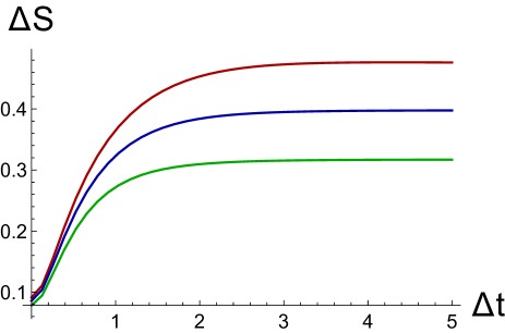
Figure 1: The evolution of the entanglement entropy for the semi-infinite system $x>0$. In this plot $\mu=0.1$, $\varepsilon=0.25$. Curves of different colors correspond to $M=0.5,1,2$ from top to bottom respectively.

In Fig.1 we present the evolution of the entanglement entropy of the semi-infinite subsystem $x>0$. In contrast to the case $T=0$ where the entanglement shows the unbounded logarithmic growth at late time for $T>0$ evolution entanglement saturates to constant value after some time.

4 Action complexity

Consider now how the CA conjecture works in our setup. For simplicity consider the probe particle approximation. This means that we neglect the backreaction of the particle. This implies that the action of our system consists of the gravity action on the static background and the particle action. The model of the particle falling on the black hole in the probe approximation still serves as a nontrivial model dual of precursor perturbation evolving in quantum system at finite temperature (also see the CA probe approximation for the string in $AdS$ in Nagasaki-1 ,Nagasaki-2 ). Following the CA prescription the complexity of the state at time $\tau$ is proportional to the on-shell gravitational and matter action restricted to the special region bounded by null rays emanating from the boundary at time $\tau$. This region is called the Wheeler-de-Witt(WdW) patch and the action $I_{\text{WdW}}$ in this patch is related to the complexity as

$$\Delta{{\cal C}}_{CA}=\frac{I_{\text{WdW}}}{\pi}.$$ (15)

In the probe approximation the time-dependent part of the complexity is the particle action swept by the WdW patch. The probe limit is easily generalized from the $AdS_{3}$ case to general dimension. Null rays bounding the WdW patch corresponding to the state at boundary time $\tau$ has the form

$$z=\pm z_{h}\tanh\frac{t-\tau}{z_{h}}.$$ (16)

Massive particle action $S$ between time moments $t_{1}$ and $t_{2}$ is given by

$$S=-mL\int_{t_{1}}^{t_{2}}\frac{2\bar{E}}{\left(\bar{E}^{2}z_{h}^{2}+1\right)\cosh\left(\frac{2t}{z_{h}}\right)-\bar{E}^{2}z_{h}^{2}+1}dt,$$ (17)

$$\bar{E}=\frac{E}{mL}.$$ (18)

The intersection of the WdW patch and the particle worldline is presented in Fig.2.

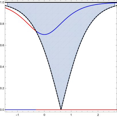
Figure 2: The WdW patch of the state at time moment $\tau=0.62$ corresponds to the blue zone. The contributing part of the worldline is show by the blue curve, red curve corresponds to the part the does not contribute. Here $z_{h}=1$.

Note, that from Fig.2 one can see that the complexity of the state depends on times $t<0$ (in Fig.2 blue part of the worldline curve extends to the region $t<0$). Remind, that quench position is $\tau=0$ and $x=0$. This means, that according to the canonical CA prescription the complexity of the state after quench strongly depends on the preparation protocol of the state. Also this could be the drawback of the particular holographic model of local quench. Note that this model has time-reversal symmetry (also see the discussion on the related issue in Ageev-quench ; Ageev-quench-2 ). For $\tau>0$ time $t_{1}$ in the formula (17) is given by

$$t_{1}=z_{h}\log\left(\sqrt{\frac{\left(2z_{h}\sqrt{\left(z_{h}^{2}-\varepsilon^{2}\right)\sinh^{2}\left(\frac{\tau}{z_{h}}\right)}-\varepsilon^{2}\right)\left(\sinh\left(\frac{\tau}{z_{h}}\right)+\cosh\left(\frac{\tau}{z_{h}}\right)\right)}{\left(2z_{h}^{2}-\varepsilon^{2}\right)\sinh\left(\frac{\tau}{z_{h}}\right)+\varepsilon^{2}\cosh\left(\frac{\tau}{z_{h}}\right)}}\right),$$ (19)

and $t_{2}\rightarrow\infty$. After integration the explicit formula for the complexity growth has the form

$$\Delta{{\cal C}}=-\frac{mL}{\pi}\left(\text{arccot}\left(\frac{2\pi T}{\bar{E}}\right)+\text{arccot}\left(\frac{2\pi T\sinh(2\pi T\tau)}{\sqrt{\bar{E}^{2}+4\pi^{2}T^{2}}-\bar{E}\cosh(2\pi T\tau)}\right)\right).$$ (20)

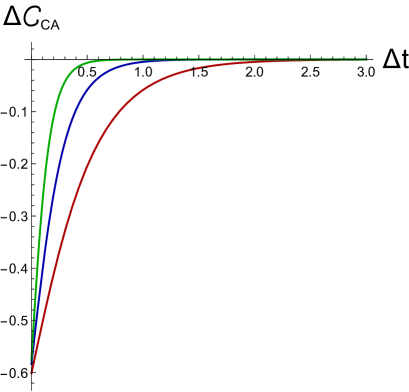
Figure 3: The growth of the CA complexity after a local quench calculated in a probe approximation. Green curve corresponds to the temperature $T=1.5$, blue one to $T=0.8$ and red one to $T=0.8$. The energy of the particle $E=0.25$ is fixed. In this plot we assume that the complexity is normalized, i.e. $\Delta{\cal C}_{CA}=\Delta{\cal C}_{CA}/(mL)$.

At the initial time moment $\tau\rightarrow 0$ the complexity exhibits the linear growth of the form

$$\Delta{{\cal C}}\approx-h\left(1+\frac{2h}{\pi}\text{arccot}\left(\frac{4h\pi T}{E}\right)\right)+\frac{\left(E+\sqrt{E^{2}+16h^{2}\pi^{2}T^{2}}\right)}{\pi}\tau,$$ (21)

where we used $m=2h/L$. For the limit $T\rightarrow 0$ we reproduce the result of Ageev-quench ; Ageev-quench-2 where the saturation of Lloyds bound at the initial time moment $\tau\rightarrow 0$ after perturbation was found. The temperature $T>0$ correction to the complexification rate at $\tau\rightarrow 0$ has the form

$$\frac{d\Delta{{\cal C}}}{dt}\approx\frac{2E}{\pi}+\frac{8h^{2}\pi T^{2}}{E}.$$ (22)

From (22) we see that temperature corrections lead to the violation of the Lloyd bound for all values of temperature. The complexity for subsystems has the qualitative behaviour similar to that one observed in Ageev-quench ; Ageev-quench-2 so we do not analyze it here in details.

5 Volume complexity

To calculate the CV complexity for the stationary dual background one have to find the volume enclosed by the minimal hypersurface spanned on the boundary at time $\tau$. There are different versions of covariant generalizations of the CV complexity proposal. In this paper we use the approximation similar to that of described in Sect.3 for the entanglement entropy. We approximate the volume complexity as

$${\cal C}_{CV}=\frac{{\cal V}}{GL},$$ (23)

where ${\cal V}$ is the volume of the constant time slice of background with the metric $g$ at the fixed time $\tau$

$${\cal V}=\int\int\left(\sqrt{\det\Sigma_{\tau}}-\frac{1}{z^{2}\sqrt{1-Mz^{2}}}\right)dxdz.$$ (24)

Here $\Sigma_{\tau}$ is the constant time slice volume form and $\Sigma_{\tau}$ is renormalized with respect to the constant time slice volume of the BTZ black hole ($\mu=0$).

 

To get some qualitative understanding of the gravitational dynamics of this model we present plot of $\Sigma_{\tau}$ in Fig.4. We see that at the inital time moment $\tau=0$ gravitational perturbation starts from the boundary $z=0$. Then the perturbation propagates to the horizon. Near the horizon at some time it splits into two parts consisting of two large tails touching the boundary approximately at $\tau=x$. Each tail become more dense closer to horizon. In the near-horizon zone they form kind of very dense gravitational perturbation. The whole late-time structure looks like ”wormhole” connecting position of two ”quasiparticles” in the boundary theory.

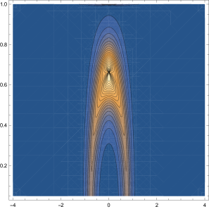
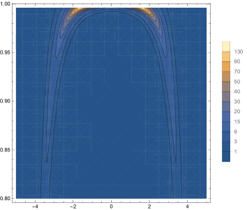
Figure 4: The density of the (renormalized) volume $\Sigma$ with $\mu=0.1$, $M=1$, $\varepsilon=0.25$. The left plot corresponds to $\tau=0.75$ and the right one to $\tau=4$.

Now let us turn to the description of the complexity growth of the total state using formula (23). Calculating this integral numerically we get the time dependence with fixed $\varepsilon$, $\mu$ and $M$. We present the result of the calculation in Fig.5. We see, that at the initial stage $\tau\rightarrow 0$ we get the quadratic growth.

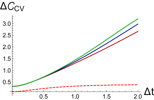
Figure 5: The CV complexity evolution of the total system for different values of temperature. Different solid curves correspond to different colors: $M=1$ (red curve), $M=1.5$ (blue curve) and $M=2$ (green curve) with the parameter values $\varepsilon=0.25$ and $\mu=0.1$. Dashed line corresponds to the entanglement evolution for the semi-infinite system $x>0$ with $M=1$. Note, that here we plot the rescaled CV complexity, i.e. ${\cal C}_{CV}\rightarrow{\cal C}_{CV}\cdot GL$

This is the common point when the dual description involves geometric quantities like the hypersurfaces stretched from the boundary. After the quadratic growth there is the regime of linear unbounded growth of the complexity $\Delta{\cal C}$. In the case of $T=0$ we see that this growth is not linear. The late time linear growth is the consequence of the fast unbounded growth of the gravitational perturbation that spreads over the black hole background.

Let us outline now how this is reflected in the behaviour of the subsystem CV complexity. First let us consider the single interval as the subsystem. The evolution is similar to the total system case except times $t\approx\ell$ where one can observe sharp decay of complexity to the equilibrium values. When $\ell\rightarrow\infty$ the point of decay is moving to $t\rightarrow\infty$ and we get an infinite linear growth corresponding to the linear growth of the total system. By naive dimensional analysis one can estimate this universal linear growth (of volume) as

$$\Delta{\cal V}\sim\frac{\mu M}{\varepsilon}\cdot t$$ (25)

and the numerical calculations with small $\varepsilon$ and $\mu$ shows that this relation takes place. Using this result one derive the linear growth of complexity in the form

$$\Delta{\cal C}\sim 32\pi^{2}T^{2}\sqrt{E^{2}+\pi^{2}h^{2}T^{2}}\cdot t$$ (26)

which violates the Lloyds bound for some values of $T$ and $h$.

Now let us consider the complexity evolution for two disjoint intervals. In this case the comparison of the complexity of this subsystem with the entanglement evolution shows the difference between these two quantities. For simplicity we take two intervals of the length $\ell$ separated by the distance $d$ located symmetric with respect to the quench point $x=0$. We present the evolution of entanglement and complexity for this system in Fig.6.

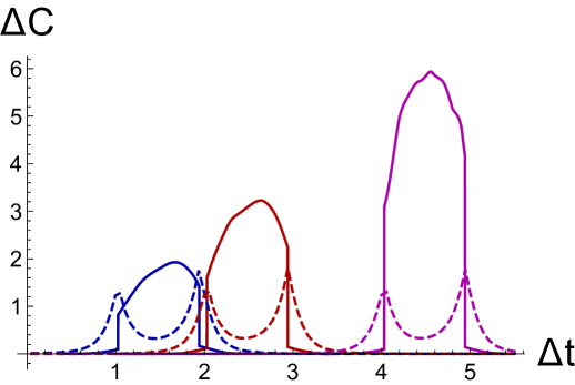
Figure 6: The CV complexity evolution(solid curves) and the entanglement entropy(dashed curve) for two disjoint intervals subsystem. The blue curves correspond to subsystem $x\in(-2,1)\cup(1,2)$, red curves to $x\in(-3,-2)\cup(2,3)$ and the magenta ones to $x\in(-5,-4)\cup(4,5)$. The entanglement entropy values are rescaled in 20 times to compare with the complexity and the complexity is rescaled as ${\cal C}_{CV}\rightarrow{\cal C}_{CV}\cdot GL$.

The entanglement evolution shows two sharp peaks approximately at times $\tau_{1}=d/2$ and $\tau_{2}=d/2+\ell$. Between these two times the entanglement has have minimum approximately at $\tau_{3}=d/2+\ell/2$. There are two sets of competing HRT surfaces connecting intervals - the ”disjoint” set corresponding to the geodesics spanned on the interval on each side of quench separately and the ”connected” set corresponding to the geodesics spanned on the endpoints of different intervals. On the early and late (before the first peak and after the last peak in the entanglement) stages of evolution the disconnected set dominates. This leads to the slow growth and decay of complexity at these stages. However in the intermediate regime between $\tau_{1}$ and $\tau_{2}$ the complexity exhibits the discontinous jump, then fast saturation to the maximum and rapid decay approximately at time corresponding to entanglement minimum. For $d\rightarrow\infty$ the maximal value of complexity is growing (in contrast to the $T=0$ where this growth is very slow for large $d$).

6 Discussion and summary

This paper is devoted to the study of the holographic complexity of a finite temperature state in two-dimensional conformal field theory that evolves after the perturbation by the local precursor. This precursor is the primary operator in the CFT with the scaling dimension $h$. From the holographic viewpoint this process is described by the point particle falling on the one-sided planar BTZ black hole horizon. The exact metric for this process is known explicitly. We calculate the CA and the CV complexity evolution in this holographic background. We make the approximate calculation for both CA and CV prescriptions. For the CA proposal we restrict ourselves to the case of probe particle approximation. We find the explicit formula describing the evolution of the action complexity. The CA evolution consists of the linear growth stage and the saturation at the late times. Instead of the saturation one can expects expect here the unbounded linear growth as different works predict Susskind:2018pmk , Stanford:2014jda . To get the late time linear growth one has to involve additional assumptions. There are different examples existing in the literature where one has to involve additional considerations to get the desired linear growth of the system. These examples are different dual models of the one-dimensional strongly coupled systems Brown:2018bms . In Brown:2018bms one introduces the special boundary terms in the action and in Alishahiha:2018swh one uses the finite bulk cutoff to get linear growth. It would be interesting to investigate the modification of our setup to get the linear late time growth. Also this calculation is performed in the approximate regime. So taking into account the gravitational backreaction effects may change the situation and produce the desired linear growth behaviour from the first principles.

As in thermofield state the CV conjecture calculation demonstrates the late time unbounded linear growth without any additional considerations. However in contrast to the CA conjecture the CV complexity shows the initial quadratic growth usually corresponding to the equilibration of the local correlations in the system. We give the simple estimate of the linear growth coefficient and find, that it violates Lloyds bound for some temperature values. The intuitive picture of dynamics of geometrical quantities in this model is as follows. After the quench gravitational perturbation evolves and get to the black hole horizon position. After that the perturbation splits in two localized ”tubes” connected through the near-horizon region. Of course this calculation is performed in the constant time approximation, so there is a question of the regime of validity of this approximation. The picture shown here also supports the idea, that the gravitational contribution may change the CA evolution in the desired way. Finally we compare the entanglement and complexity evolution for system of disjoint intervals and find, that the (local) minimum of the entanglement is realized when the complexity is maximal. This raises question about how the complexity is related to the quasiparticle picture. Remember, that the entanglement is in good correspondence with this picture. The further investigations and possible extensions of this work include the comparison of the TFD state perturbed by local operator with one-sided black hole. Also it is important to consider the inclusion of the gravitational correction to the CA computation. Also it is interesting to compare with different complexity results concerning non-equilibrium states developed in QFT1 -QFT2 .

References

- (1) S. Ryu and T. Takayanagi, “Holographic derivation of entanglement entropy from AdS/CFT,” Phys. Rev. Lett. 96, 181602 (2006) [hep-th/0603001].
- (2) M. Van Raamsdonk, “Building up spacetime with quantum entanglement,” Gen. Rel. Grav. 42, 2323 (2010) [Int. J. Mod. Phys. D 19, 2429 (2010)] [arXiv:1005.3035 [hep-th]].
- (3) B. Swingle, “Entanglement Renormalization and Holography,” Phys. Rev. D 86, 065007 (2012) [arXiv:0905.1317 [cond-mat.str-el]].
- (4) L. Susskind, “Computational Complexity and Black Hole Horizons,” Fortsch. Phys. 64, 24 (2016) doi:10.1002/prop.201500092 [arXiv:1403.5695 [hep-th], arXiv:1402.5674 [hep-th]].
- (5) L. Susskind, “Why do Things Fall?,” arXiv:1802.01198 [hep-th].
- (6) D. S. Ageev and I. Y. Aref’eva, “When things stop falling, chaos is suppressed,” JHEP 1901, 100 (2019) [JHEP 2019, 100 (2020)] doi:10.1007/JHEP01(2019)100 [arXiv:1806.05574 [hep-th]].
- (7) L. Susskind, “Three Lectures on Complexity and Black Holes,” arXiv:1810.11563 [hep-th].
- (8) D. Stanford and L. Susskind, “Complexity and Shock Wave Geometries,” Phys. Rev. D 90, no. 12, 126007 (2014) doi:10.1103/PhysRevD.90.126007 [arXiv:1406.2678 [hep-th]].
- (9) A. R. Brown, D. A. Roberts, L. Susskind, B. Swingle and Y. Zhao, “Holographic Complexity Equals Bulk Action?,” Phys. Rev. Lett. 116, no. 19, 191301 (2016) doi:10.1103/PhysRevLett.116.191301 [arXiv:1509.07876 [hep-th]].
- (10) A. R. Brown, D. A. Roberts, L. Susskind, B. Swingle and Y. Zhao, “Complexity, action, and black holes,” Phys. Rev. D 93, no. 8, 086006 (2016) doi:10.1103/PhysRevD.93.086006 [arXiv:1512.04993 [hep-th]].
- (11) M. Alishahiha, “Holographic Complexity,” Phys. Rev. D 92, no. 12, 126009 (2015) doi:10.1103/PhysRevD.92.126009 [arXiv:1509.06614 [hep-th]].
- (12) P. Caputa, N. Kundu, M. Miyaji, T. Takayanagi and K. Watanabe, “Anti-de Sitter Space from Optimization of Path Integrals in Conformal Field Theories,” Phys. Rev. Lett. 119, no. 7, 071602 (2017) doi:10.1103/PhysRevLett.119.071602 [arXiv:1703.00456 [hep-th]].
- (13) P. Caputa, N. Kundu, M. Miyaji, T. Takayanagi and K. Watanabe, “Liouville Action as Path-Integral Complexity: From Continuous Tensor Networks to AdS/CFT,” JHEP 1711, 097 (2017) doi:10.1007/JHEP11(2017)097 [arXiv:1706.07056 [hep-th]].
- (14) T. Takayanagi, “Holographic Spacetimes as Quantum Circuits of Path-Integrations,” arXiv:1808.09072 [hep-th].
- (15) R. Abt, J. Erdmenger, H. Hinrichsen, C. M. Melby-Thompson, R. Meyer, C. Northe and I. A. Reyes, ’‘Topological Complexity in AdS3/CFT2,” arXiv:1710.01327 [hep-th].
- (16) S. Banerjee, J. Erdmenger and D. Sarkar, “Connecting Fisher information to bulk entanglement in holography,” arXiv:1701.02319 [hep-th].
- (17) D. S. Ageev, I. Y. Aref’eva, A. A. Bagrov and M. I. Katsnelson, “Holographic local quench and effective complexity,” JHEP 1808, 071 (2018) [arXiv:1803.11162 [hep-th]].
- (18) D. Ageev, “Holography, quantum complexity and quantum chaos in different models,” EPJ Web Conf. 191, 06006 (2018). doi:10.1051/epjconf/201819106006
- (19) K. Nagasaki, “Complexity of AdS5 black holes with a rotating string,” Phys. Rev. D 96, no. 12, 126018 (2017) [arXiv:1707.08376 [hep-th]].
- (20) K. Nagasaki, “Complexity growth of rotating black holes with a probe string,” arXiv:1807.01088 [hep-th].
- (21) D. Carmi, S. Chapman, H. Marrochio, R. C. Myers and S. Sugishita, “On the Time Dependence of Holographic Complexity,” JHEP 1711, 188 (2017) doi:10.1007/JHEP11(2017)188 [arXiv:1709.10184 [hep-th]].
- (22) S. Chapman, H. Marrochio and R. C. Myers, “Complexity of Formation in Holography,” JHEP 1701, 062 (2017) doi:10.1007/JHEP01(2017)062 [arXiv:1610.08063 [hep-th]].
- (23) B. Swingle and Y. Wang, “Holographic Complexity of Einstein-Maxwell-Dilaton Gravity,” arXiv:1712.09826 [hep-th].
- (24) S. A. Hosseini Mansoori and M. M. Qaemmaqami, “Complexity Growth, Butterfly Velocity and Black hole Thermodynamics,” arXiv:1711.09749 [hep-th].
- (25) Y. Ling, Y. Liu and C. Y. Zhang, “Holographic Subregion Complexity in Einstein-Born-Infeld theory,” Eur. Phys. J. C 79, no. 3, 194 (2019) doi:10.1140/epjc/s10052-019-6696-5 [arXiv:1808.10169 [hep-th]].
- (26) Y. S. An and R. H. Peng, “The effect of Dilaton on the holographic complexity growth,” arXiv:1801.03638 [hep-th].
- (27) M. Alishahiha, A. Faraji Astaneh, M. R. Mohammadi Mozaffar and A. Mollabashi, “Complexity Growth with Lifshitz Scaling and Hyperscaling Violation,” arXiv:1802.06740 [hep-th].
- (28) M. Moosa, “Divergences in the rate of complexification,” arXiv:1712.07137 [hep-th].
- (29) M. Moosa, “Evolution of Complexity Following a Global Quench,” arXiv:1711.02668 [hep-th].
- (30) B. Chen, W. M. Li, R. Q. Yang, C. Y. Zhang and S. J. Zhang, “Holographic subregion complexity under a thermal quench,” arXiv:1803.06680 [hep-th].
- (31) S. Chapman, H. Marrochio and R. C. Myers, “Holographic complexity in Vaidya spacetimes. Part I,” JHEP 1806, 046 (2018) doi:10.1007/JHEP06(2018)046 [arXiv:1804.07410 [hep-th]].
- (32) S. Chapman, H. Marrochio and R. C. Myers, “Holographic complexity in Vaidya spacetimes. Part II,” JHEP 1806, 114 (2018) doi:10.1007/JHEP06(2018)114 [arXiv:1805.07262 [hep-th]].
- (33) Z. Y. Fan and M. Guo, “Holographic complexity under a global quantum quench,” arXiv:1811.01473 [hep-th].
- (34) P. Calabrese and J. Cardy, “Entanglement and correlation functions following a local quench: a conformal field theory approach,” J. Stat. Mech. 0710, no. 10, P10004 (2007) [arXiv:0708.3750 [quant-ph]].
- (35) M. Nozaki, T. Numasawa and T. Takayanagi, “Holographic Local Quenches and Entanglement Density,” JHEP 1305, 080 (2013) [arXiv:1302.5703 [hep-th]].
- (36) T. Shimaji, T. Takayanagi and Z. Wei, “Holographic Quantum Circuits from Splitting/Joining Local Quenches,” arXiv:1812.01176 [hep-th].
- (37) C. T. Asplund, A. Bernamonti, F. Galli and T. Hartman, “Holographic Entanglement Entropy from 2d CFT: Heavy States and Local Quenches,” JHEP 1502, 171 (2015) [arXiv:1410.1392 [hep-th]].
- (38) P. Caputa, J.Simon, A.Stikonas, T. Takayanagi and K.Watanabe, ”Scrambling time from local perturbations of the eternal BTZ black hole,” JHEP 1508, 011 (2015) [arXiv:1503.08161 [hep-th]].
- (39) P.Caputa, J.Simon, A.Stikonas and T.Takayanagi, “Quantum Entanglement of Localized Excited States at Finite Temperature,” JHEP 1501, 102 (2015) [arXiv:1410.2287 [hep-th]].
- (40) D. S. Ageev, I. Y. Aref’eva and M. D. Tikhanovskaya, “(1+1)-Correlators and moving massive defects,” Theor. Math. Phys. 188, no. 1, 1038 (2016) [Teor. Mat. Fiz. 188, no. 1, 85 (2016)] [arXiv:1512.03362 [hep-th]].
- (41) D. S. Ageev and I. Y. Aref’eva, “Holographic instant conformal symmetry breaking by colliding conical defects,” Theor. Math. Phys. 189, no. 3, 1742 (2016) [Teor. Mat. Fiz. 189, no. 3, 389 (2016)] [arXiv:1512.03363 [hep-th]].
- (42) A. Jahn and T. Takayanagi, J. Phys. A 51, no. 1, 015401 (2018) [arXiv:1705.04705 [hep-th]].
- (43) J. R. David, S. Khetrapal and S. P. Kumar, “Local quenches and quantum chaos from higher spin perturbations,” JHEP 1710, 156 (2017) [arXiv:1707.07166 [hep-th]].
- (44) T. De Jonckheere and J. Lindgren, “Entanglement entropy in inhomogeneous quenches in AdS3/CFT2,” arXiv:1803.04718 [hep-th].
- (45) A. R. Brown, H. Gharibyan, H. W. Lin, L. Susskind, L. Thorlacius and Y. Zhao, “The Case of the Missing Gates: Complexity of Jackiw-Teitelboim Gravity,” arXiv:1810.08741 [hep-th].
- (46) A. Akhavan, M. Alishahiha, A. Naseh and H. Zolfi, “Complexity and Behind the Horizon Cut Off,” JHEP 1812, 090 (2018) doi:10.1007/JHEP12(2018)090 [arXiv:1810.12015 [hep-th]].
- (47) M. Alishahiha, “On Complexity of Jackiw-Teitelboim Gravity,” arXiv:1811.09028 [hep-th].
- (48) D. W. F. Alves and G. Camilo, “Evolution of complexity following a quantum quench in free field theory,” JHEP 1806, 029 (2018) doi:10.1007/JHEP06(2018)029 [arXiv:1804.00107 [hep-th]].
- (49) H. A. Camargo, P. Caputa, D. Das, M. P. Heller and R. Jefferson, “Complexity as a novel probe of quantum quenches: universal scalings and purifications,” arXiv:1807.07075 [hep-th].
- (50) S. Chapman, J. Eisert, L. Hackl, M. P. Heller, R. Jefferson, H. Marrochio and R. C. Myers, “Complexity and entanglement for thermofield double states,” arXiv:1810.05151 [hep-th].
- (51) T. Ali, A. Bhattacharyya, S. Shajidul Haque, E. H. Kim and N. Moynihan, “Time Evolution of Complexity: A Critique of Three Methods,” arXiv:1810.02734 [hep-th].