Deep learning detection of transients

Abstract

The next generation of observatories will facilitate the discovery of new types of astrophysical transients. The detection of such phenomena, whose characteristics are presently poorly constrained, will hinge on the ability to perform blind searches. We present a new algorithm for this purpose, based on deep learning. We incorporate two approaches, utilising anomaly detection and classification techniques. The first is model-independent, avoiding the use of background modelling and instrument simulations. The second method enables targeted searches, relying on generic spectral and temporal patterns as input. We compare our methodology with the existing approach to serendipitous detection of gamma-ray transients. The algorithm is shown to be more robust, especially for non-trivial spectral features. We use our framework to derive the detection prospects of low-luminosity gamma-ray bursts with the upcoming Cherenkov Telescope Array. Our method is an unbiased, completely data-driven approach for multiwavelength and multi-messenger transient detection.

1 Introduction

Transient astrophysical phenomena at high energies present us with the opportunity to explore a broad range of fundamental physics. Recent years have seen a revolution of the field, with the first joint detections of gamma rays ($\gamma\text{-rays}$) and gravitational waves (GWs) (Abbott et al., 2017); evidence for $\gamma\text{-ray}$ association with neutrinos (Aartsen et al., 2018); and the first detection of a $\gamma\text{-ray}$ burst (GRB) at sub-TeV energies (Mirzoyan, 2019). This has led to a wealth of scientific output, touching e.g., on the formation of heavy elements; the physics of GRBs; and the properties of accelerators of cosmic rays (Abbott et al., 2017; Rosswog et al., 2018; Rodrigues et al., 2018).

One of the interesting source populations that might be fully unveiled in the near future is that of low-luminosity $\gamma\text{-ray}$ bursts (LL-GRBs) (Liang et al., 2007; Virgili et al., 2009). LL-GRBs are a sub-class of the population of long GRBs, which has been connected to mildly relativistic supernovae (Cano et al., 2017). Compared to most bursts, LL-GRBs are distinguished by low isotropic equivalent luminosities, generally considered for ${{10^{{46}}}<{L_{\gamma,\text{iso}}}<{10^{{49}}}~{}\text{erg}\,\sec^{-1}}$. Only a small number of LL-GRBs have been observed to date. However, there are indications that their observable rate in the local Universe (redshift, ${z<0.1}$) is high, of the order of ${150\,\mathrm{Gpc}^{-3}\,\mathrm{yr}^{-1}}$ (Sun et al., 2015).

The exact nature of the prospective very-high-energy (VHE) emission from LL-GRBs is uncertain. However, the motivation to search for such events is high. For one, LL-GRBs may be detectable as sources of gravitational waves (Howell et al., 2011). Additionally, compared to their higher-luminosity counterparts, LL-GRBs are favoured as the sources of ultra high energy cosmic rays. Primarily, this is because LL-GRBs present an optimal balance between processes of particle acceleration and of energy loss (Murase et al., 2008; Zhang et al., 2018; Boncioli et al., 2018). They therefore provide an efficient environment for cosmic ray generation and escape. Correspondingly, LL-GRBs represent a unique multi-messenger window into the extreme energy regimes of $\gamma\text{-rays}$, cosmic rays, neutrinos, and GWs.

Existing ground- and space-based observatories are capable of detecting $\gamma\text{-rays}$ within the regime relevant for LL-GRBs. However, their current detection is very challenging. For instance, Fermi-GBM is not optimised for the detection of LL-GRBs, due to their low peak synchrotron energies (Sun et al., 2015); for Fermi-LAT, detection is unlikely given the poor sensitivity to transients on short time scales (Abdollahi et al., 2017). Conversely, imaging atmospheric Cherenkov telescopes (IACTs) can perform well on short intervals. However, the sensitivity of the current generation of instruments to transient phenomena below ${100~{}\text{GeV}}$ is very limited.

The upcoming Cherenkov Telescope Array (CTA) will significantly improve upon the current facilities. Specifically, CTA will provide a large field-of-view (FoV) and improved energy resolution. It will also allow observation of $\gamma\text{-rays}$ down to ${\sim\kern-1.99997pt20~{}\text{GeV}}$, which will be critical for LL-GRBs. The rate of observable LL-GRBs under the duty-cycle of CTA is estimated as up to $1$ detection per-month (based on their relative number density with regards to high-luminosity GRBs (Inoue et al., 2013)). As such, they are appealing targets for real-time searches.

LL-GRBs and other putative transient populations are not well constrained by current observations. In order to maximise the potential of online searches, the corresponding algorithms will need to make as few model assumptions as possible. Accordingly, data-driven analysis methods have the potential to significantly enhance the existing infrastructure.

In the following study we present a new method, intended for the detection of transient events. Our algorithm is based on deep learning, using recurrent neural networks. It employs two complementary approaches, optimised for both model-independent and targeted searches.

Both training and evaluation of our estimator are computationally inexpensive, allowing for detection of transients on second time scales with insignificant latency. Our method can therefore be incorporated as part of real-time analyses. As such, it will be used by CTA to transmit transient event alerts to the astronomical community. These alerts will facilitate effective multiwavelength / multi-messenger followup of the discovered events, which will be crucial for their interpretation.

We use our algorithm to make the first predictions for serendipitous VHE detection of LL-GRBs. We perform a scan of the parameter space of events, identifying those that would be within reach of CTA. Compared to the existing state of the art, we achieve higher detection rates for non-trivial source types.

While we illustrate our new approach using $\gamma\text{-ray}$ sources, it is by design generic and model independent. The methodology is not restricted to a specific energy regime, type of input, or time scale. In particular, it is well suited for multiwavelength and multi-messenger searches, where different observable are combined. It can therefore easily be adapted for many other transient searches.

2 Existing detection methodologies

2.1 Techniques for $\gamma\text{-ray}$ source detection

IACTs must exclude a significant amount of background, mostly originating from cosmic rays (Berge, D. et al., 2007; Funk, 2015). Unless extremely short time intervals are considered, this background is irreducible, and must be corrected for on average.

Different approaches are used in order to identify excesses of reconstructed events. One common method is to define on- and off-regions of observation within the same FoV (Aharonian et al., 2001; Berge, D. et al., 2007). For this kind of analysis, a source is searched for within the on-region, while the off-region(s) are assumed to only contain background events. Contemporaneous measurements within off-regions are used to estimate the number density of background events, which is then subtracted from counts in the on-region.

This type of method has the advantage that the background is derived directly from the data. However, the off-regions are by construction separated from the position of the source. The method is therefore susceptible to uncertainties on e.g., the homogeneity of the performance of the camera.

Another approach is to perform a likelihood analysis, which requires explicit modelling of both the source and the background (Knodlseder et al., 2016). In a common application of this technique, the background is estimated by a fit over the entire FoV, covering an area where no sources are expected to exist.

Such methodology is very powerful, as it naturally allows for sophisticated background modelling. However, it has the disadvantage of strongly depending on the accuracy of instrument response functions (IRFs), which encapsulate the effective area, radial acceptance, point spread function and energy dispersion of the instrument.

For both approaches, one must usually make additional assumptions on the spectral and temporal properties of the source (Weiner et al., 2017). This may limit the discovery potential for unexpected transient types.

2.2 Transient detection strategies

The nominal strategy for observing GRBs with CTA is to follow external alerts, which would be generated by other instruments (Acharya et al., 2017). This is mainly driven by the low rate of occurrence of high-luminosity GRBs (Inoue et al., 2013), which makes their serendipitous discovery by CTA unlikely.

In the case of LL-GRBs, the potentially high rates motivate blind searches. These would be performed within the FoV of CTA during normal operations, not as a response to an alert. We follow this approach exclusively in the current study. Our nominal strategy is to conduct continuous searches. In the most simple scenario, these would be performed in multiple independent regions of interest (RoIs), covering the entire FoV.

Real-time discovery of transients with IACTs is challenging. Existing methods have to control a large number of effects, such as undetected sources within the FoV; imperfect modelling of galactic foregrounds or of the effect of stars; and uncertainties on the combination of data from multiple observation epochs (which may be necessary for background estimation). The latter in particular implies that one must account for many parameters, e.g., the zenith and azimuth angles of observation; the night sky background; and changes in the density and transparency of the atmosphere (Aleksić et al., 2012).

It is foreseen that CTA will use dedicated IRFs for min–hour observation periods, which would account for changing observing conditions. Such simulations would be generated with some delay after data taking. Correspondingly, the online analysis will be based on IRFs compatible with averaged anticipated conditions.

The focus of this paper is the development of new detection methods. In light of the challenges discussed above, our objective is to minimise the dependence on modelling, as well as the influence of observational effects.

3 New detection methods

This study presents two novel transients detection algorithms, denoted in the following as anomaly detection, and classification.

Anomaly detection represents a model-independent approach, where transient events are identified based on their divergence from the expected background. This simple methodology is completely data-driven, and is able to adapt to real-time evolution of the background.

Our approach has a clear advantage over traditional methods; the background model is derived in-situ, and from the same RoI as for the source. Anomaly detection is therefore completely decoupled from the simulation of the instrument. It is also insensitive to uncertainties on modelling of the background, the atmosphere, or any of the other artefacts mentioned above.

Our second new method employs classification. In this case, we train an estimator to identify transient patterns. While less model-independent than anomaly detection, the classification approach increases the sensitivity of specific searches, such as for LL-GRBs.

Compared to existing methods, classification has several advantages. Similarly to anomaly detection, data from different RoIs need not be mixed. In addition, the time structure of transient events is naturally incorporated as a part of the training process, avoiding the need for explicit modelling. Finally, simple training examples may be used as the basis for detecting sources with more complicated intrinsic spectra, as illustrated below.

3.1 Recurrent neural network estimator

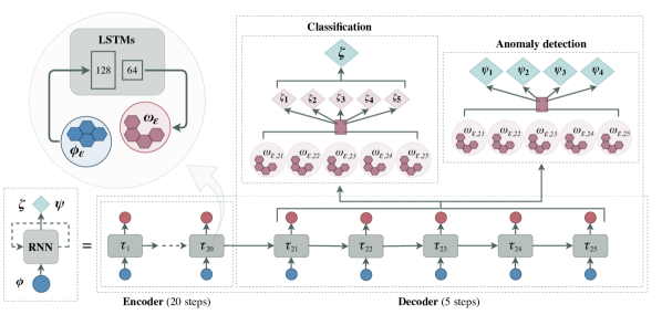
Figure 1: Schematic design of the RNN used in this study. The unrolled representation may be decomposed into an encoder and a decoder. These respectively represent $20$ and $5$ time steps, $\tau$, of LSTM units (rectangles). Each LSTM comprises two layers of $128$ and $64$ hidden units. The input data, $\phi$, (blue circles) make up $4$ numbers for each time step (blue hexagons), corresponding to event counts in four energy bins, $\epsilon$. The direct output of the LSTMs, $\omega_{\epsilon,\tau}$, (red hexagons) are predictions for event counts for each step and energy bin. The output of the RNN (diamonds) depends on the implementation. For the case of anomaly detection, the output, $\psi_{1-4}$, provides the predicted background counts for each of the energy bins, integrated over the decoder time steps. The output of the classification method, $\zeta$, may be calibrated into a probability density function.

Machine learning is widely used in astronomy (Sadeh et al., 2016; Krause et al., 2017; Reis et al., 2018). Deep learning, and in particular convolutional neural networks, have shown great promise. Successful applications include optical and $\gamma\text{-ray}$ object classification, and transient searches in e.g., images and radio signals (Kim et al., 2018; Domínguez Sánchez et al., 2019; Sedaghat & Mahabal, 2018; Gieseke et al., 2017; Erdmann et al., 2019).

In the current study, we utilise a recurrent neural network (RNN), made up of long short-term memory (LSTM) units. RNNs are a type of artificial neural network, which is well suited for time series analysis. They have numerous applications, ranging from natural language translation (Sutskever et al., 2014) to denoising of GW signals (Shen et al., 2017).

The connections between the LSTM nodes in an RNN form a directed graph, representing a sequence of steps in time. Outputs from each time step are fed as input to the next, in addition to the respective temporal data.

In principle, RNNs may be used to make predictions for arbitrarily distant inputs. For computational reasons, it is common to implement unrolled versions of RNNs. These contain a fixed number of steps, i.e., a fixed number of inputs and outputs. For a review of deep learning and RNNs, see LeCun et al. (2015).

The neural network used in this study is implemented with the open-source software, tensorflow (Abadi et al., 2015). The architecture of the RNN is illustrated in Figure 1.

The network accepts an input which corresponds to $25$ time steps, each representing a ${1~{}\sec}$ interval of $\gamma\text{-ray}$ data. The different steps are implemented as RNN cells. A cell is composed of a pair of LSTM layers, respectively comprising $128$ and $64$ hidden units. The hidden units are conceptually similar to nodes in a feedforward neural network. As such, they represent the set of parameters which are tuned during training.

The network may be decomposed into two elements, an encoder and a decoder. The encoder receives $20$ time steps as input. A potential transient signal event is then searched for within the $5$ time steps associated with the decoder.

The input data corresponding to a given time step are a list of features. These are respectively denoted by ${\{\bm{\phi}^{\mathrm{enc}}_{\epsilon,\tau}\}_{\tau\in 1-20}}$ and ${\{\bm{\phi}^{\mathrm{dec}}_{\epsilon,\tau}\}_{\tau\in 21-25}}$, for the encoder and decoder time steps. In the current study, the features are event counts in $4$ logarithmically-spaced energy bins within ${30<E_{\mathrm{\gamma}}<200~{}\text{GeV}}$ (starting slightly above the lower energy threshold of CTA).

The inputs to the encoder are assumed to correspond to background-only counts in all cases. The input to the decoder and the output of the network depend on the type of inference being used, as discussed below.

We did not explore the full parameter space of possible RNN architectures. Rather, the chosen temporal and energetic representation is motivated by the expected properties of LL-GRBs, and is intended to illustrate our methodology. It is possible that better performance could be achieved with a different configuration, which we leave for future work.

We also note that the architecture is easily generalisable to different time scales. It may also incorporate additional features, such as data-quality metrics; per-event background rejection probabilities; information related to the weather; optical observations of the perspective transient; and detected artefacts (e.g., meteors). Such observables may take the form of single numbers, probability density functions, CCD images, etc.

3.2 Anomaly detection

Using anomaly detection, transient events are identified by detecting significant deviations of observed event counts, compared to the expected background. Poissonian statistics are assumed for both the background and the signal models. The corresponding probability distributions are $p^{\mathrm{bck}}_{\mathrm{anm}}$ and $p^{\mathrm{sig}}_{\mathrm{anm}}$, where ${p^{\mathrm{bck/sig}}_{\mathrm{anm}}(k|\lambda)=e^{-\lambda}}\lambda^{k}/k!$, given the rate parameter, $\lambda$.

The background in this case is derived in-situ. This is done using data exclusively from within the RoI for the source. In the most simple application, spectral modelling of the source is not needed, and a simple top-hat function is assumed for the temporal behaviour. More sophisticated assumptions on the source may be taken. For instance, one could weight the event counts of the different time steps by an assumed temporal trend (Weiner et al., 2017). We do not take such an approach here, as this would potentially limit the detectability of unexpected transient patterns.

The network is trained using background-only events for all $25$ time steps. Training events can in general be derived from simulations, or from historical or near-contemporaneous data. This methodology is particularly powerful, as the estimator will continuously be optimised (retrained) using real-time data.

The network is trained by optimizing (minimising) a loss function. The latter encodes the difference between the output of the network and the intended outcome. The purpose of the anomaly detection RNN is to directly predict the number of counts inside the RoI. In the current study, we chose to integrate the output of the decoder across the $5$ time steps. The corresponding predictions for the $4$ energy bins are denoted by ${\{\bm{\psi}_{\epsilon}\}_{\epsilon\in 1-4}}$. The loss function for training is therefore defined as the absolute difference between observed event counts and $\bm{\psi}_{\epsilon}$ predictions.

When the trained network is used to evaluate data, it receives a sequence of $25$ input features, $\bm{\phi}_{\epsilon,\tau}$. In the case that a transient event occurs, the signal features, $\bm{\phi}^{\mathrm{dec}}_{\epsilon,\tau}$, (time steps, ${\tau_{21}-\tau_{25}}$) may correspond to higher event rates. Such a pattern is never introduced as part of the training, and may be incompatible with the background-only model of the RNN. We therefore replace the $5$ steps, $\bm{\phi}^{\mathrm{dec}}_{\epsilon,\tau}$, with inputs from the encoder. The predictions from the trained network are then used to estimate the rate parameters of the Poissonian background distributions, ${\{\bm{\lambda}^{\mathrm{bck}}_{\epsilon}\}_{\epsilon\in 1-4}}$.

Up to this point in the analysis, we have only utilised data from the encoding phase of the network (${\tau_{1}-\tau_{20}}$). In order to estimate the Poissonian probability function of the signal model, we use $\bm{\phi}^{\mathrm{dec}}_{\epsilon}$. The latter stand for the counts of the perspective signal in each energy bin, integrated over time steps, ${\tau_{21}-\tau_{25}}$.

The Poissonian rate parameters of the signal are estimated for the different energy bins as

$$\bm{\lambda}^{\mathrm{sig}}_{\epsilon}=\max\{\bm{\phi}^{\mathrm{dec}}_{\epsilon},\,\bm{\kappa}_{\epsilon}\}.$$ (1)

The parameter, $\bm{\kappa}_{\epsilon}$, is nominally selected as ${\bm{\kappa}_{\epsilon}=\bm{\lambda}^{\mathrm{bck}}_{\epsilon}}$ in the current study. Setting the background rate as a lower limit for the signal ensures that downward fluctuations of $\bm{\phi}^{\mathrm{dec}}_{\epsilon}$ moderate the significance of a detection; this reduces the rate of spurious detections by a large fraction. It is also possible to use higher values of $\bm{\kappa}_{\epsilon}$, corresponding to increasingly conservative detection thresholds. For instance, one may choose to set ${\bm{\kappa}_{\epsilon}=(\bm{\lambda}^{\mathrm{bck}}_{\epsilon}+n_{\mathrm{min}})}$. On average, this would be akin to requiring that at least ${n_{\mathrm{min}}}$ $\gamma\text{-rays}$ above background are detected in each energy bin.

The test statistic for detecting a transient signal within the ${\tau_{21}-\tau_{25}}$ time interval can finally be derived, reading

$$\mathrm{TS}_{\mathrm{anm}}=-2\log\left(\frac{p^{\mathrm{bck}}_{\mathrm{anm}}(\bm{\phi}^{\mathrm{dec}}_{\epsilon}|\bm{\lambda}^{\mathrm{bck}}_{\epsilon})}{p^{\mathrm{sig}}_{\mathrm{anm}}(\bm{\phi}^{\mathrm{dec}}_{\epsilon}|\bm{\lambda}^{\mathrm{sig}}_{\epsilon})}\right).$$ (2)

3.3 Classification

Instead of using the RNN to predict background counts within different temporal/energy bins, the estimator may be used to directly classify transient events. In this case, an external layer is added to the decoder, mapping the output (of event counts) into $5$ logits, denoted by $\bm{\zeta}_{\tau}$. Each logit represents a probability density function for an event to belong to the signal class, based on a single decoder time step (within ${t_{21}-t_{25}}$).

The network is trained using labelled examples of background and signal events. Correspondingly, the output logits represent the inferred probability that an event belongs to the signal class. The loss function which is optimised during training represents the accuracy of all logits. The combined accuracy is calculated as a weighted average across the $5$ time steps, where the weights are themselves optimised during training. Consequently, the unique time structure of signal events drives the training.

The output of the RNN, $\zeta$, is the inferred classification metric for a given event (see Fig. 3(a) below). We define the test statistic for identifying a signal event as

$$\mathrm{TS}_{\mathrm{clas}}=-2\log\left(\frac{\zeta_{\mathrm{bck}}}{\zeta_{\mathrm{sig}}}\right),$$ (3)

following the prescription of Cranmer et al. (2015). Strictly speaking, the combined classification metric, $\zeta$, is not a logit (for computational reasons it is not normalised to span the interval ${[0,1]}$). However, the distributions of $\zeta$ can be calibrated to serve as probability density functions for each class.

In order to prevent distortions due to binning effects, we do not use the value of $\zeta$ directly. Rather, we first fit the distributions of $\zeta$ with kernel density estimators (KDEs). A KDE is a non-parametric method for parametrising probability density functions (Parzen, 1962). It depends only on a single bandwidth parameter, $h_{\mathrm{KDE}}$. The bandwidth defines a smoothing scale for the distributions of $\zeta$, and is optimised to the results of the training.

4 GRB simulations

We demonstrate the application of our algorithm, by making predictions for serendipitous detection of LL-GRBs with CTA, as described in the following.

4.1 Spectral models

Due to their low luminosities, LL-GRBs are expected to be characterised by low bulk Lorentz factors (of the order of $10$), and low values of their peak spectral energy distribution (${\sim\kern-1.99997pt10-100~{}\text{keV}}$ in the observer frame) (Ghirlanda et al., 2018). Consequently, their synchrotron emission is not likely to be detectable at multi-GeV energies. While a higher-energy inverse-Compton component might in fact be observable by CTA, it is also possible that this signal is suppressed due to absorption inside the source (Rudolph et al., In prep.). Despite these uncertainties, it remains important to perform VHE searches for LL-GRBs. Any detection will significantly advance our understanding.

In order to simulate the possible $\gamma\text{-ray}$ signatures of LL-GRBs, we use the following reference events: GRBs ${\mathrm{080916C}}$, ${\mathrm{090323}}$, ${\mathrm{090510}}$, ${\mathrm{090902B}}$, and ${\mathrm{110731A}}$. These are all bright high-luminosity GRBs, which have been detected at high energies with Fermi-LAT (see  Ajello et al. (2013) and references therein).

The selected reference events are best fit by different types of models e.g., a Band function (Band et al., 1993), a power law (PL), or a PL with an exponential cutoff. It is therefore possible that the spectral components detected by Fermi-LAT are in fact a part of the afterglow, rather than of the prompt phase of these GRBs. In the following, we assume that this is not the case. That is, we interpret the GeV emission as an extension of e.g., the Band model to high energies. In such a case, it is possible to predict the corresponding prompt GeV component of LL-GRBs, based on a simplistic scaling of the flux (cf. Inoue et al. (2013)).

We begin by randomly shifting the reference GRBs in redshift and luminosity to the expected ranges for LL-GRBs. In order to simulate the signals at GeV energies, we nominally assume a simple spectral/temporal PL model,

$$M_{\mathrm{PL}}(E,t)=k_{0}\left(\frac{E}{E_{0}}\right)^{-\Gamma}t^{-\tau}.$$ (4)

The prefactor and pivot energy, $k_{0}$ and $E_{0}$, are derived directly from the flux of the GRB. The spectral index, $\Gamma$, and temporal decay index, $\tau$, are randomly selected for each event, uniformly distributed within $1.9<\Gamma<2.7$ and $0.8<\tau<2$. These properties generally correspond to the expectations for the low-luminosity population. We only consider those bursts which exhibit durations of the order of tens of seconds, excluding the population of ultra-long GRBs (Levan et al., 2013).

We also simulate bursts having an exponential cutoff. The corresponding spectral models are parametrised as

$$M_{\mathrm{EC}}(E)=M_{\mathrm{PL}}\cdot\exp\left(-\frac{E}{E_{\text{cut}}}\right),$$ (5)

where $E_{\text{cut}}$ is the cutoff energy.

The observed spectra of cosmological VHE sources are distorted by interactions with low-energy photons from the extragalactic background light (EBL). The bursts considered in this study have low redshift and $\gamma\text{-ray}$ energies (compared to most high-luminosity GRBs). Consequently, the effect of the EBL is not expected to be important. We compared our results using several EBL models (Franceschini et al., 2008; Dominguez et al., 2011; Gilmore et al., 2012). We found that the effect of using a particular model or none at all is indeed insignificant for our sample.

4.2 Event simulation

We generate IACT events using the open-source software, ctools (Knodlseder et al., 2016). The latter is one of the proposed analysis frameworks for CTA, which implements the likelihood method discussed in subsection 2.1. The Northern array of CTA is simulated using the publicly available IRFs (version prod3b-v1). In the current study, we exclusively use IRFs optimised for ${30~{}\min}$ observations at zenith angles of ${\sim\kern-1.99997pt20\degree}$. We leave the comprehensive characterisation of LL-GRB detectability under different observing conditions for future studies.

We simulate two samples, one composed entirely of background counts, and the other including GRBs. All bursts are modelled as PL spectra (Eq. 4), unless otherwise indicated (cf. Fig. 5(c)). The energy range of $\gamma\text{-rays}$ is restricted to reconstructed values, ${30<E_{\gamma}<200~{}\text{GeV}}$, where most of the emission from LL-GRBs is expected to be detected.

The RoI for the simulation is chosen as a circular region with a radius of ${0.25\degree}$, centred at the position of the source. The latter is displaced by ${0.5\degree}$ from the centre of the FoV. For each sequence, we derive $\bm{\phi}_{\epsilon,\tau}$ by counting the number of reconstructed $\gamma\text{-ray}$-events within the RoI for each time step and energy bin.

The counts, $\bm{\phi}_{\epsilon,\tau}$, are susceptible to fluctuation due to imperfect $\gamma\text{-ray}$ reconstruction, as well as to uncertainties on the IRFs. In particular, energy dispersion below ${\sim\kern-1.99997pt50~{}\text{GeV}}$ may result in migration between bins, and can change the energy threshold of the analysis. We studied these effects by allowing $10\%$ variation on the IRFs. We found that the propagated uncertainties do not significantly affect our results.

As part of a realistic online analysis, searches would be performed as sliding windows in time. For the purpose of the current study, we only conduct searches over the ${5~{}\sec}$ intervals that coincide with the beginning of bursts in the signal sample. This is done regardless of the value of the randomised temporal decay parameter, $\tau$. We accordingly simulate a ${25~{}\sec}$ interval for each burst. The first ${20~{}\sec}$ (before the GRB emission would begin) are fed into the encoder of the RNN ($\bm{\phi}^{\mathrm{enc}}_{\epsilon,\tau}$), and the next ${5}$ into the decoder ($\bm{\phi}^{\mathrm{dec}}_{\epsilon,\tau}$).

4.3 Detection significance

Performing continuous blind searches for transient events incurs a penalty on the test statistic. To correct for the number of trials, we assume the following connection between pre- and post-trials probabilities, ${p_{\mathrm{post}}=1-\left(1-p_{\mathrm{pre}}\right)^{n_{\mathrm{trial}}}}$ (Biller, 1996).

The number of trials, ${n_{\mathrm{trial}}}$, represents both the frequency of searches and the number of RoIs within the FoV of CTA. The former corresponds to $100$ hours of observations at ${1~{}\sec}$ search intervals in the current study. The latter accounts for a conservative ${100}$ simultaneous observations every second. In total, we consider ${{3.6}\cdot 10^{{7}}}$ trials.

We compare the results of our new algorithm with the test statistic computed by ctools, $\mathrm{TS}_{\mathrm{ctl}}$, taken as a proxy for the likelihood methodology. The $\mathrm{TS}_{\mathrm{ctl}}$ metric is derived exclusively from the final ${5~{}\sec}$ interval, during which the GRB would be active.

5 Results

As the benchmark performance metric for simulated GRBs, we define the detectability, ${p_{\mathrm{det}}=\left<\rho_{\mathrm{det}}\right>}$, for

$$\begin{matrix}\rho_{\mathrm{det}}(t)=&\left\{\begin{matrix}0\;,&t<\mathrm{TS}_{5\sigma}\\ 1\;,&t\geq\mathrm{TS}_{5\sigma}\end{matrix}\right..&\\ \end{matrix}$$ (6)

Here $t$ represents the test statistic derived for a given detection method; ${\mathrm{TS}_{5\sigma}}$ is the corresponding threshold for a $5\sigma$ detection, where e.g., for a model with a single degree of freedom, ${\mathrm{TS}_{5\sigma}=25}$ (Wilks, 1938).

The detectability metric is averaged over samples with different combinations of parameters (e.g., spectral indices and redshifts). The absolute value of $p_{\mathrm{det}}$ depends on the sample composition, which in this case is not physically motivated by a GRB luminosity function. However, $p_{\mathrm{det}}$ may be used to identify the most promising regions of the parameter space. It can also serve for objective comparison between the different detection methods.

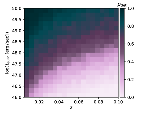
Figure 2: The detectability metric, $p_{\mathrm{det}}$, derived with ctools, after accounting for trials. The simulation sample includes different combinations of redshift, $z$, and isotropic equivalent luminosity, ${L_{\gamma,\text{iso}}}$, spanning the expected properties of LL-GRBs, assuming PL spectral models.

The distribution of ${p_{\mathrm{det}}(\mathrm{TS}_{\mathrm{ctl}})}$ as a function of redshift, $z$, and isotropic equivalent luminosity, ${L_{\gamma,\text{iso}}}$, is shown in Fig. 2. Much of the relevant parameter space of LL-GRBs is available for CTA. Lower redshift values and higher GRB luminosities are correlated with higher event fluxes. As expected, these also correspond to higher probabilities for a burst to be detected.

Using the trained RNN in the classification mode, we derive the distributions of the classification metric, $\zeta$, for the background and signal samples, as shown in Fig. 3(a). The distributions are used to fit a KDE estimator. We chose the KDE bandwidth such that the resulting distribution of $\mathrm{TS}_{\mathrm{clas}}$ is smooth for values ${>10}$. The corresponding relation between $\mathrm{TS}_{\mathrm{clas}}$ and $\zeta$ is presented in Fig. 3(b).

((a))

((b))

Figure 3: Parametrisation of the performance of the trained classification method. LABEL:sub@FIGclsDist Distributions of the classification metric, $\zeta$, for the signal and background samples, as indicated. LABEL:sub@FIGclsTs The parametrised classification test statistic, $\mathrm{TS}_{\mathrm{clas}}$, (see Eq. 3) as a function of $\zeta$, before and after the correction for trials. The dashed-dotted horizontal line highlights the value, $\mathrm{TS}=25$.

We now proceed to evaluate the test statistics for the various methods. Fig. 4 shows $f_{\mathrm{det}}$, the fraction of events with a $\mathrm{TS}$ value larger than a given threshold, as a function of this threshold. One may compare the performance of the different detection methods for signal events.

We find that ctools and the anomaly detection achieve comparable significance distributions. The two methods manage to detect a similar fraction of the events, with slightly better performance by ctools. The baseline equivalence between the methods is expected, as both utilise Poissonian statistics. However, ctools gains significance from a successful fit to the assumed spectral model of the source, while no such assumptions are taken for the anomaly detection. This relative gain in performance is balanced out when the intrinsic spectral model of the source is more complicated, as discussed below.

Considering the classification approach, the performance is better than that of ctools, with a relative improvement in detectability of ${\sim\kern-1.99997pt10\%}$ on average. A direct comparison between these two techniques is less straightforward. In general, the assumed temporal properties of a transient may be incorporated into a likelihood analysis. As we did not take this approach in the current study, the RNN has a clear advantage over ctools. In addition, the relative weights between the different energy and time bins are optimised as a part of training. The classification method is therefore less sensitive to the intrinsic spectra of the sources, which results in increased sensitivity.

It is important to verify that the new detection methods do not produce spurious detections, and that the corresponding test statistics are properly mapped to significance. We therefore evaluate the different algorithms on the background sample, and compare them to the reference ctools distribution.

As shown in Fig. 4(b), the anomaly detection and classification methods produce comparable or better (lower) rates of fake detections. The classification method in particular exhibits an order of magnitude relative improvement over ctools. For the given sample of ${10^{{6}}}$ background simulations, none of the methods exceed a pre-trials $\mathrm{TS}$ value of $20$, or a post-trials value of $1$.

((a))

((b))

Figure 4: Dependence of $f_{\mathrm{det}}$, the fraction of events with a $\mathrm{TS}$ value larger than a given threshold, on the value of the threshold. The different detections methods are compared, derived for the signal LABEL:sub@FIGintgrTsSigSig and background LABEL:sub@FIGintgrTsSigBck samples, as indicated. The full lines in either figure correspond to the pre-trials test statistic. The dashed lines in LABEL:sub@FIGintgrTsSigSig represent $f_{\mathrm{det}}$ after accounting for trials, where in LABEL:sub@FIGintgrTsSigBck we found ${f_{\mathrm{det}}(\mathrm{TS}>1)=0}$ post-trials in all cases. For clarity, the relations are truncated to the range, ${1<\mathrm{TS}<100}$, where the pre-trials background distributions in LABEL:sub@FIGintgrTsSigBck do not extend beyond ${\mathrm{TS}\approx 20}$. The dashed-dotted vertical line in LABEL:sub@FIGintgrTsSigSig highlights the value, $\mathrm{TS}=25$.

((a))

((b))

((c))

Figure 5: Dependence of $p_{\mathrm{det}}$ on selected simulation parameters, after accounting for trials, where the shaded regions correspond to ${1\sigma}$ uncertainties on the values of $p_{\mathrm{det}}$, derived using the bootstrap method. LABEL:sub@FIGpdetTimeIndex-LABEL:sub@FIGpdetSpecIndex Dependence of $p_{\mathrm{det}}$ on the temporal and spectral indices of GRBs, $\tau$ and $\Gamma$, for bursts simulated as PLs (see Eq. 4), for the different detection methods, as indicated. LABEL:sub@FIGpdetExCutoff Dependence of $p_{\mathrm{det}}$ on the cutoff energy, $E_{\text{cut}}$, for bursts simulated as exponentially cutoff PLs (see Eq. 5). Two alternative models are used for detection with ctools, an exponentially cutoff PL, and a simple PL, as indicated. The classification method had exclusively been trained using simple PL examples in all cases.

We investigated different combinations of GRB spectral and temporal parameters. The most important of the latter are those which moderate the duration of the burst, and the extension of the spectra to multi-GeV energies; namely, the temporal and spectral indices, and the possible existence of a cutoff. The dependence of $p_{\mathrm{det}}$ on these parameters is shown in Fig. 5. One may observe that our new methods match or improve upon the performance of ctools. As expected, longer-lasting and harder spectra are more likely to be detected by all algorithms.

Fig. 5(c) shows the detectability of LL-GRBs which are simulated with exponentially cutoff PL spectra. For cutoff energies, ${E_{\text{cut}}<1~{}\text{GeV}}$, bursts are undetectable within the chosen reconstructed energy range (${30<E_{\gamma}<200~{}\text{GeV}}$). Above this threshold, the performance depends on the given detection method.

The figure illustrates the main motivation for using our RNN. A search with ctools, under the assumption of an exponentially cutoff power law, was able to match the performance of the RNN. However, the results of the likelihood analysis were not robust (the fits had to be tuned with particular choices of parameter initialisation and allowed ranges). This is mainly due to the relatively low number of $\gamma\text{-rays}$ that are available to be fit.

In practice, the problem of testing complicated models as part of an online search is compounded, as many possible extensions are possible. This implies that one would need to make additional assumptions; and to test different parameters that are not initially well constrained. It is therefore doubtful that such a search would be successful as part of a realistic detection strategy.

Instead, it is likely that simple PL models will be assumed for the initial blind search. Our new algorithms are specifically designed to have as little dependence as possible on the intrinsic spectra of sources. As illustrated here, they perform comparably better than ctools in this scenario.

In principle, the classification results may be improved, by training with labelled examples of both PL and exponentially cutoff GRBs. In order to minimise modelling, we only used simple PL bursts as examples in the current study,. Despite this, the classification is shown to be robust. It outperforms the likelihood method (for ${E_{\text{cut}}>30~{}\text{GeV}}$), even when confronted with events representing unexpected intrinsic models.

6 Summary

In this study, we present a new approach for source detection. Our algorithm is based on deep learning, utilising recurrent neural networks, which are ideally suited for time series analysis. The model can be used to evaluate observation sequences of second time scales with insignificant latency. The choice of technology is therefore particularly fitting for real-time searches.

We have developed two methods, based on anomaly detection and classification techniques. Anomaly detection represents a model-independent approach, where transient events are identified based on their divergence from the expected background. The method is completely data-driven. We thus avoid the need for background modelling, as well as for explicit characterisation of the state of the instrument.

The classification method allows one to perform targeted searches. In this case, the RNN is trained to identify generic transient patterns. The estimator provides high detection rates while maintaining low fake rates.

We have compared the performance of our new methods to that of existing techniques, where the background and signal models are explicitly defined. With the new algorithms, we are able to match or improve upon the existing methods, while using fewer assumptions. This is especially important when non-trivial source models are considered, e.g., exponentially cutoff power law spectra. In such cases, we have shown that our approach is more robust.

We have used our new methodology to derive the detection prospects of LL-GRBs with CTA. Provided that LL-GRBs indeed exhibit VHE emission above ${\sim\kern-1.99997pt30~{}\text{GeV}}$, CTA will be sensitive to a wide range of events. Depending on their redshift, bursts with isotropic equivalent luminosities as low as ${{10^{{46}}}~{}\text{erg}\,\sec^{-1}}$ could be detected.

While we have used LL-GRBs as a benchmark source class, the methodology presented here is applicable for any transient search. Our RNN estimator can trivially be generalised for searches over different time scales. It can also be used with different types of inputs, unrelated to photon counts, e.g., images and other analysis products. As such it is ideally suited for multiwavelength and multi-messenger transient searches.

References

- Aartsen et al. (2018) Aartsen, M. G., et al. 2018, Science, 361, 147, doi: 10.1126/science.aat2890
- Abadi et al. (2015) Abadi, M., Agarwal, A., Barham, P., et al. 2015
- Abbott et al. (2017) Abbott, B. P., et al. 2017, Phys. Rev. Lett., 119, 161101, doi: 10.1103/PhysRevLett.119.161101
- Abbott et al. (2017) Abbott, B. P., Abbott, R., Abbott, T. D., et al. 2017, ApJ, 848, L13, doi: 10.3847/2041-8213/aa920c
- Abdollahi et al. (2017) Abdollahi, S., et al. 2017, Astrophys. J., 846, 34, doi: 10.3847/1538-4357/aa8092
- Acharya et al. (2017) Acharya, B. S., et al. 2017. https://arxiv.org/abs/1709.07997
- Aharonian et al. (2001) Aharonian, F., et al. 2001, A&A, 370, 112, doi: 10.1051/0004-6361:20010243
- Ajello et al. (2013) Ajello, M., et al. 2013, Astrophys. J. Suppl., 209, 11, doi: 10.1088/0067-0049/209/1/11
- Aleksić et al. (2012) Aleksić, J., et al. 2012, Astroparticle Physics, 35, 435, doi: 10.1016/j.astropartphys.2011.11.007
- Band et al. (1993) Band, D., Matteson, J., Ford, L., et al. 1993, ApJ, 413, 281, doi: 10.1086/172995
- Berge, D. et al. (2007) Berge, D., Funk, S., & Hinton, J. 2007, A&A, 466, 1219, doi: 10.1051/0004-6361:20066674
- Biller (1996) Biller, S. 1996, Astroparticle Physics, 4, 285 , doi: https://doi.org/10.1016/0927-6505(95)00036-4
- Boncioli et al. (2018) Boncioli, D., Biehl, D., & Winter, W. 2018, ArXiv e-prints. https://arxiv.org/abs/1808.07481
- Cano et al. (2017) Cano, Z., Wang, S.-Q., Dai, Z.-G., & Wu, X.-F. 2017, Adv. Astron., 2017, 8929054, doi: 10.1155/2017/8929054
- Cranmer et al. (2015) Cranmer, K., Pavez, J., & Louppe, G. 2015. https://arxiv.org/abs/1506.02169
- Dominguez et al. (2011) Dominguez, A., Primack, J. R., Rosario, D. J., et al. 2011, Monthly Notices of the Royal Astronomical Society, 410, 2556, doi: 10.1111/j.1365-2966.2010.17631.x
- Domínguez Sánchez et al. (2019) Domínguez Sánchez, H., Huertas-Company, M., Bernardi, M., et al. 2019, MNRAS, 484, 93, doi: 10.1093/mnras/sty3497
- Erdmann et al. (2019) Erdmann, M., Schlueter, F., & Smida, R. 2019. https://arxiv.org/abs/1901.04079
- Franceschini et al. (2008) Franceschini, A., Rodighiero, G., & Vaccari, M. 2008, Astron. Astrophys., 487, 837, doi: 10.1051/0004-6361:200809691
- Funk (2015) Funk, S. 2015, Annual Review of Nuclear and Particle Science, 65, 245, doi: 10.1146/annurev-nucl-102014-022036
- Ghirlanda et al. (2018) Ghirlanda, G., Nappo, F., Ghisellini, G., et al. 2018, Astron. Astrophys., 609, A112, doi: 10.1051/0004-6361/201731598
- Gieseke et al. (2017) Gieseke, F., Bloemen, S., van den Bogaard, C., et al. 2017, MNRAS, 472, 3101, doi: 10.1093/mnras/stx2161
- Gilmore et al. (2012) Gilmore, R. C., Somerville, R. S., Primack, J. R., & Dominguez, A. 2012, Monthly Notices of the Royal Astronomical Society, 422, 3189, doi: 10.1111/j.1365-2966.2012.20841.x
- Howell et al. (2011) Howell, E., Regimbau, T., Corsi, A., Coward, D., & Burman, R. 2011, Mon. Not. Roy. Astron. Soc., 410, 2123, doi: 10.1111/j.1365-2966.2010.17585.x
- Inoue et al. (2013) Inoue, S., et al. 2013, Astropart. Phys., 43, 252, doi: 10.1016/j.astropartphys.2013.01.004
- Kim et al. (2018) Kim, B., Humensky, B., Nieto, D., et al. 2018, in APS April Meeting Abstracts, Vol. 2018, L01.031
- Knodlseder et al. (2016) Knodlseder, J., et al. 2016, Astron. Astrophys., 593, A1, doi: 10.1051/0004-6361/201628822
- Krause et al. (2017) Krause, M., Pueschel, E., & Maier, G. 2017, Astroparticle Physics, 89, 1, doi: 10.1016/j.astropartphys.2017.01.004
- LeCun et al. (2015) LeCun, Y., Bengio, Y., & Hinton, G. 2015, Nature, 521, 436 EP
- Levan et al. (2013) Levan, A. J., et al. 2013, Astrophys. J., 781, 13, doi: 10.1088/0004-637X/781/1/13
- Liang et al. (2007) Liang, E., Zhang, B., & Dai, Z. G. 2007, Astrophys. J., 662, 1111, doi: 10.1086/517959
- Mirzoyan (2019) Mirzoyan, R. 2019, The Astronomer’s Telegram, 12390
- Murase et al. (2008) Murase, K., Ioka, K., Nagataki, S., & Nakamura, T. 2008, Phys. Rev. D, 78, 023005, doi: 10.1103/PhysRevD.78.023005
- Parzen (1962) Parzen, E. 1962, Ann. Math. Statist., 33, 1065, doi: 10.1214/aoms/1177704472
- Reis et al. (2018) Reis, I., Poznanski, D., Baron, D., Zasowski, G., & Shahaf, S. 2018, MNRAS, 476, 2117, doi: 10.1093/mnras/sty348
- Rodrigues et al. (2018) Rodrigues, X., Biehl, D., Boncioli, D., & Taylor, A. M. 2018, ArXiv e-prints. https://arxiv.org/abs/1806.01624
- Rosswog et al. (2018) Rosswog, S., Sollerman, J., Feindt, U., et al. 2018, A&A, 615, A132, doi: 10.1051/0004-6361/201732117
- Rudolph et al. (In prep.) Rudolph, et al. In prep.
- Sadeh et al. (2016) Sadeh, I., Abdalla, F. B., & Lahav, O. 2016, doi: 10.1088/1538-3873/128/968/104502
- Sedaghat & Mahabal (2018) Sedaghat, N., & Mahabal, A. 2018, MNRAS, 476, 5365, doi: 10.1093/mnras/sty613
- Shen et al. (2017) Shen, H., George, D., Huerta, E. A., & Zhao, Z. 2017. https://arxiv.org/abs/1711.09919
- Sun et al. (2015) Sun, H., Zhang, B., & Li, Z. 2015, Astrophys. J., 812, 33, doi: 10.1088/0004-637X/812/1/33
- Sutskever et al. (2014) Sutskever, I., Vinyals, O., & Le, Q. V. 2014, in NIPS’14 (MIT Press), 3104–3112. http://dl.acm.org/citation.cfm?id=2969033.2969173
- Virgili et al. (2009) Virgili, F., Liang, E., & Zhang, B. 2009, Mon. Not. Roy. Astron. Soc., 392, 91, doi: 10.1111/j.1365-2966.2008.14063.x
- Weiner et al. (2017) Weiner, O. M., Humensky, T. B., Mukherjee, R., & Santander, M. 2017, Astroparticle Physics, 93, 1, doi: 10.1016/j.astropartphys.2017.05.004
- Wilks (1938) Wilks, S. S. 1938, Annals Math. Statist., 9, 60, doi: 10.1214/aoms/1177732360
- Zhang et al. (2018) Zhang, B. T., Murase, K., Kimura, S. S., Horiuchi, S., & Mészáros, P. 2018, Phys. Rev. D, 97, 083010, doi: 10.1103/PhysRevD.97.083010