Abstract

We consider a novel quantum field-theoretical approach to the description of processes passing at finite space-time intervals based on the Feynman diagram technique in the coordinate representation. The most known processes of this type are neutrino and neutral kaon oscillations. The experimental setting of these processes requires one to adjust the rules of passing to the momentum representation in the Feynman diagram technique in accordance with it, which leads to a modification of the Feynman propagator in the momentum representation. The approach does not make use of wave packets, both initial and final particle states are described by plane waves, which simplifies the calculations considerably. We consider neutrino oscillation processes, where the neutrinos are produced in three-particle weak decays of nuclei and detected in the charged-current interaction with nuclei or in the charged- and neutral-current interactions with electrons. Particular examples are considered and it is shown that the momentum spread of the produced neutrinos and the energy dependence of the differential cross section of the detection process result in the suppression of neutrino oscillation, which is characterized by a coherence length specific for a pair of production and detection processes. This coherence length turns out to be much less than the coherence length in the standard quantum-mechanical approach defined by the quantum uncertainty of neutrino momentum.

1 Introduction

The Standard Model allows one to describe a great amount of different elementary particle interaction processes with a high accuracy in the framework of the perturbative S-matrix formalism and the Feynman diagram technique. However, there is a number of phenomena which cannot be described in the framework of the standard perturbation theory. In particular, these are strange neutral meson oscillations and neutrino oscillations, which take place at finite macroscopic space and time intervals. These phenomena are described either in the quantum mechanical approach in terms of plane waves [1, 2, 3, 4, 5, 6, 7] or in the QM or QFT approaches in terms of wave packets [8, 9, 10, 11, 12]. The first one is based on the notion of the states with definite flavour (definite strangeness) which are superpositions of the states with definite mass. It is postulated that it is the flavour states that are produced in the weak interaction, and their evolution in time underlies the oscillations. However, in the plane wave approximation, the production of states without definite mass leads to violation of energy-momentum conservation, which was widely discussed in the literature [8, 9, 10, 11, 12]. This problem can be solved in the framework of the wave-packet treatment [5], but the price is an essential complication of the corresponding calculations.

An alternative quantum field-theoretical description put forward in [8] and developed in [9, 10] explains the neutrino oscillations by interference of the amplitudes of processes mediated by different virtual neutrinos with definite masses. In the framework of this description there are no problems with energy-momentum conservation, but the calculations of amplitudes turn out to be rather complicated because of the necessity to use wave packets in order to describe a localization of particles or nuclei. The calculation procedure is essentially different from the standard calculations in the Feynman diagram technique in the momentum representation. This is due to the standard S-matrix formalism of QFT not being convenient for describing processes at finite distances and finite time intervals.

In what follows, we show that neutrino oscillations may be consistently described in the framework of quantum field theory using only plane waves, which simplifies the calculations considerably. Nevertheless, in the developed approach energy-momentum is conserved as well. The idea of the novel approach is to adjust the standard S-matrix formalism for describing the processes of finite duration. We consider the processes of production and detection as a whole, use the Feynman diagram technique in the coordinate representation to write down the amplitude and then pass to the momentum representation in a way, which corresponds to the experimental setting. Effectively it leads to a modification of the Feynman propagator in the momentum representation, while all the other Feynman rules in the momentum representation are kept intact. The approach is based on two papers by R. Feynman [13, 14] and developed in papers [15, 16, 17]. In the present paper, in the framework of the proposed approach, we consider the processes of neutrino oscillations, where the neutrinos produced in weak decays of nuclei are detected either in the weak charged-current interaction with nuclei or in both the charged- and neutral-current interactions with electrons.

An important characteristic of neutrino oscillation processes is the coherence length, which is the measure of fading out of the oscillation pattern with distance. It appears in the quantum-mechanical description of neutrino oscillation in terms of wave packets due to the momentum uncertainty of the neutrino states. Meanwhile, in the framework of this approach one considers only the neutrino states with the same expectation value of momentum, which enters the expressions for the oscillation lengths. This means that a beam of such neutrinos can be viewed as a monochromatic one at the distances from the source much less than the coherence lengths. However, the neutrinos produced in three-particle weak decays of nuclei are not monochromatic, and the spread of neutrino momenta can also affect the oscillation pattern.

In the quantum field-theoretical approach to neutrino oscillations under consideration there is no momentum uncertainty of neutrino states, because all the particles, just like in the standard Feynman diagram technique, are described by plane waves. For this reason fading out of the oscillation pattern in this approach can result only from the momentum spread of the produced neutrinos. In what follows we examine specific examples and show how the coherence length appears in our approach and what are the differences between our approach and the standard one.

2 Neutrino oscillations in experiments with detection in the charged-current interaction only

2.1 Theory

We work in the framework of the minimal extension of the Standard Model by the right neutrino singlets. The charged-current interaction Lagrangian of the leptons takes the form

$$L_{\rm cc}=-\frac{g}{2\sqrt{2}}\left(\sum_{i,k=1}^{3}\bar{l}_{i}\gamma^{\mu}(1-\gamma^{5})U_{ik}\nu_{k}W^{-}_{\mu}+h.c.\right),$$ (1)

where $l_{i}$ is the field of the charged lepton of the $i$-th generation, $U_{ik}$ denotes the PMNS-matrix, and $\nu_{k}$ stands for the field of the neutrino state with definite mass.

Let us consider a process, where a neutrino is emitted and detected in the charged-current interaction with nuclei. In the lowest order of perturbation theory the process is described by the following diagram:

The points of production $x$ and detection $y$ are supposed to be separated by a fixed macroscopic interval. The intermediate neutrino mass eigenstate is a virtual particle and is described by the propagator in the coordinate representation. All three virtual neutrino mass eigenstates contribute to the amplitude of the process, thus the amplitude of the process corresponding to the diagram must be summed over all the three neutrino mass eigenstates, $i=1,2,3$.

As it is customary in the Feynman diagram technique, we suppose that the initial and final nuclei and particles are described by plane waves, i.e. they have definite momenta. Hence, all the three virtual neutrino eigenstates have definite momenta as well. Let us assign the 4-momenta of the particles as it is shown in the diagram, namely, $q$ is the positron 4-momentum, $k$ is the electron 4-momentum and $p_{\rm n}$ is the intermediate virtual neutrino 4-momentum. To be specific, we will suppose that the virtual $W$-bosons are produced and absorbed in the interactions with nuclei as follows: a nucleus ${{}^{A_{1}}_{Z_{1}}{\rm X}}$, which will be referred to as nucleus $1$, emits $W^{+}$-boson and turns into the nucleus ${{}^{A_{1}}_{Z_{1}-1}{\rm X}}$, which will be referred to as nucleus $1^{\prime}$, and a nucleus ${{}^{A_{2}}_{Z_{2}}{\rm X}}$, which will be referred to as nucleus $2$, absorbs $W^{+}$-boson and turns into the nucleus ${{}^{A_{2}}_{Z_{2}+1}{\rm X}}$, which will be referred to as nucleus $2^{\prime}$. Thereby the filled circles in the diagram represent the matrix elements of the weak charged hadron current

$$j_{\mu}^{(1)}\left({P^{(1)},P^{(1^{\prime})}}\right)=\left<{}^{A_{1}}_{Z_{1}-1}{\rm X}\right|j_{\mu}^{({\rm h})}\left|{}^{A_{1}}_{Z_{1}}{\rm X}\right>,\quad j_{\rho}^{(2)}\left({P^{(2)},P^{(2^{\prime})}}\right)=\left<{}^{A_{2}}_{Z_{2}+1}{\rm X}\right|j_{\rho}^{({\rm h})}\left|{}^{A_{2}}_{Z_{2}}{\rm X}\right>,$$

corresponding to nuclei $1,1^{\prime}$ and $2,2^{\prime}$; the nuclei 4-momenta are denoted by $P^{(l)}=(E^{(l)},\vec{P}^{(l)})$, $P^{(l^{\prime})}=(E^{(l^{\prime})},\vec{P}^{(l^{\prime})})$, $l=1,2$.

The amplitude in the coordinate representation corresponding to diagram (2) can be written out using the Feynman rules in the coordinate representation formulated, for example, in textbook [18]. In order to pass to the momentum representation one would have to integrate the amplitude with respect to $x$ and $y$ over Minkowski space, which would give the corresponding matrix element of the S-matrix.

However, such an integration would result in losing the information about the space-time interval between the production event and the detection event, because the experimental situation in neutrino oscillation experiments implies that the distance between the production point and the detection point along the neutrino propagation direction remains fixed. To generalize the standard S-matrix formalism to the case of processes passing at fixed distances, we have to modify the integration in such a way that it would take into account a fixed distance between the neutrino production and detection points. This can be done by introducing a delta function into the integral, which would fix the distance between these points. However, in paper [16] it was argued that it was more convenient to fix the time interval between the production and detection events by introducing the delta function $\delta(y^{0}-x^{0}-T)$ into the integral, because, for a beam of neutrinos with the same momentum, this is equivalent to fixing the distance between these events in accordance with the formula $T=Lp^{0}/|\vec{p}|$, which is often used in describing neutrino oscillation processes [5].

Having fixed the time interval between the events of production and detection, we integrate the amplitude with respect to $x$ and $y$ over Minkowski space. Thus, just like in the standard S-matrix formalism, we consider the process taking place throughout Minkowski space-time, but the time interval between the production and detection events is now fixed by the delta function. This is equivalent to replacing the standard Feynman fermion propagator in the coordinate representation $S^{\rm c}_{i}(y-x)$ by $S^{\rm c}_{i}(y-x)\delta(y^{0}-x^{0}-T)$.

The Fourier transform of this expression gives us the so-called time-dependent propagator of the neutrino mass eigenstate $\nu_{i}$ in the momentum representation, defined by the relation:

$$S^{\rm c}_{i}(p,T)=\int dx\,e^{ipx}S^{\rm c}_{i}(x)\,\delta(x^{0}-T).$$ (3)

This integral can be evaluated exactly [15, 16]:

$$S^{\rm c}_{i}\left({p,T}\right)=i\,\frac{{\hat{p}-\gamma_{0}\left({p^{0}-\sqrt{\left({p^{0}}\right)^{2}+m_{i}^{2}-p^{2}}}\right)+m_{i}}}{{2\sqrt{\left({p^{0}}\right)^{2}+m_{i}^{2}-p^{2}}}}\,e^{i\left({p^{0}-\sqrt{\left({p^{0}}\right)^{2}+m_{i}^{2}-p^{2}}}\right)T}\,,$$ (4)

where $m_{i}$ is the mass of $i$-th neutrino mass eigenstate and the standard notation $\hat{p}=\gamma_{\mu}p^{\mu}$ is used. The inverse Fourier transformation of this time-dependent propagator is well defined, which allows us to retain the standard Feynman diagram technique in the momentum representation just by replacing the Feynman propagator by the time-dependent propagator.

In paper [9] it was rigorously proved that virtual particles propagating at large macroscopic distances (or, equivalently, propagating over macroscopic times) are almost on the mass shell, which means that $|p^{2}-m_{i}^{2}|/\left({p^{0}}\right)^{2}\ll 1$. This is in accord with the structure of time-dependent propagator (4). As it was discussed in [17], formally the amplitude of a process with such a propagator corresponds to the instant registration. The process itself is considered to take time $T$ exactly. It reality, however, the registration has a non-zero duration $\Delta t$, and the amplitude constructed with time-dependent propagator (4) should be interpreted as the amplitude per unit time. In order to find the amplitude of a realistic process with the detection time $\Delta t$ one must integrate the time-dependent amplitude with respect to $T$ from $T-{{\Delta t}\mathord{\left/{\vphantom{{\Delta t}2}}\right.\kern-1.2pt}2}$ to $T+{{\Delta t}\mathord{\left/{\vphantom{{\Delta t}2}}\right.\kern-1.2pt}2}$. It reduces to the integration of propagator (4) only, which gives

$$\int\limits_{T-\Delta t/2}^{T+\Delta t/2}{S_{i}^{\rm c}\left({p,t}\right)dt}=S_{i}^{\rm c}\left({p,T}\right)\frac{{\sin\alpha}}{\alpha}\Delta t,\quad\alpha=\left({p^{0}-\sqrt{\left({p^{0}}\right)^{2}+m_{i}^{2}-p^{2}}}\right)\frac{\Delta t}{2}.$$ (5)

For large $\alpha\gg 1$ this integral is close to zero, and we can expect that the amplitude will be essentially non-zero only for those particles, for which $\alpha\simeq 0$. In this case the amplitude with the registration time ${\Delta t}$ is proportional to ${\Delta t}$, and the amplitude with $T$ fixed can really be viewed as the amplitude of the registration per unit time.

The registration time interval $\Delta t$ is macroscopically large, which means that the factor $\left({p^{0}-\sqrt{\left({p^{0}}\right)^{2}+m_{i}^{2}-p^{2}}}\right)$ should be very small. The latter is the expression of the fact that the virtual neutrino is almost on the mass shell. Thus, our approach actually gives another proof of the Grimus-Stockinger theorem [9]. Applying this result to time-dependent propagator (4), i.e neglecting $|p^{2}-m_{i}^{2}|/\left({p^{0}}\right)^{2}\ll 1$ everywhere, except in the exponential, where it is multiplied by the macroscopic time $T$, we get

$$S_{i}^{\rm c}\left({p,T}\right)=i\frac{{\hat{p}+m_{i}}}{{2p^{0}}}e^{-i\frac{{m_{i}^{2}-p^{2}}}{{2p^{0}}}T}.$$ (6)

It is this expression that will be used for the calculations hereinafter.

Now we are in a position to write down the amplitude in the momentum representation corresponding to diagram (2) in the case, when the time difference $y^{0}-x^{0}$ between the events of production and detection is fixed and equal to $T$. Since the momentum transfer in both the production and detection processes is small, one can use the approximation of Fermi’s interaction. Using the time-dependent fermion field propagator (6), where we retain the neutrino masses only in the exponential, we arrive at the amplitude summed over all the three neutrino mass eigenstates:

$$M = -i\frac{{G_{\rm F}^{\,2}}}{4{p_{\rm n}^{0}}}\sum\limits_{i=1}^{3}{\left|{U_{1i}}\right|^{2}e^{-i\frac{m_{i}^{2}-p_{\rm n}^{2}}{2p_{\rm n}^{0}}T}}\times$$

$$\times j_{\rho}^{(2)}\left({P^{(2)},P^{(2^{\prime})}}\right)\bar{u}\left(k\right)\gamma^{\rho}\left({1-\gamma^{5}}\right)\hat{p}_{\rm n}\gamma^{\mu}\left({1-\gamma^{5}}\right)v\left(q\right)j_{\mu}^{(1)}\left({P^{(1)},P^{(1^{\prime})}}\right).$$

Here and below we omit the fermion polarization indices for simplicity.

The squared modulus of the amplitude, averaged with respect to the polarizations of the incoming nuclei and summed over the polarizations of the outgoing particles and nuclei (the operation of averaging and summation is denoted by the angle brackets), factorizes in the approximation of massless neutrinos as follows:

$$\left\langle{\left|M\right|^{2}}\right\rangle = \left\langle{\left|M_{1}\right|^{2}}\right\rangle\left\langle{\left|M_{2}\right|^{2}}\right\rangle\frac{{1}}{{4\left({p^{0}_{\rm n}}\right)^{2}}}\left[{1-4\sum\limits_{\scriptstyle i,k=1\hfill\atop\scriptstyle i<k\hfill}^{3}{\left|{U_{1i}}\right|^{2}\left|{U_{1k}}\right|^{2}\sin^{2}\left({\frac{{m_{i}^{2}-m_{k}^{2}}}{{4p^{0}_{\rm n}}}T}\right)}}\right],$$ (8)

$$\left\langle{\left|M_{1}\right|^{2}}\right\rangle = 4G_{\rm F}^{\,2}\left(-{g^{\mu\nu}\left({p_{\rm n}q}\right)+\left({p_{\rm n}^{\mu}q^{\nu}+q^{\mu}p_{\rm n}^{\nu}}\right)+i\varepsilon^{\mu\nu\alpha\beta}p_{{\rm n}\alpha}q_{\beta}}\right)W_{\mu\nu}^{(1)},$$ (9)

$$\left\langle{\left|M_{2}\right|^{2}}\right\rangle = 4G_{\rm F}^{\,2}\left(-{g^{\rho\sigma}\left({p_{\rm n}k}\right)+\left({p_{\rm n}^{\rho}k^{\sigma}+k^{\rho}p_{\rm n}^{\sigma}}\right)-i\varepsilon^{\rho\sigma\alpha\beta}p_{{\rm n}\alpha}k_{\beta}}\right)W_{\rho\sigma}^{(2)},$$ (10)

where the nuclear tensors $W_{\mu\nu}^{(1)}$, $W_{\rho\sigma}^{(2)}$ characterizing the interaction of nuclei $1$ and $2$ with the virtual $W$-bosons are defined as

$$W_{\alpha\beta}^{(l)}=W_{\alpha\beta}^{(l,{\rm S})}+iW_{\alpha\beta}^{(l,{\rm A})}=\left\langle{j_{\alpha}^{(l)}\left({j_{\beta}^{(l)}}\right)^{+}}\right\rangle,\quad l=1,2,$$ (11)

their symmetrical parts $W_{\alpha\beta}^{(l,{\rm S})}$ being real and the anti-symmetrical ones $iW_{\alpha\beta}^{(l,{\rm A})}$ being imaginary.

Our next step is to find the differential probability of the process, where the intermediate neutrino momentum $p_{\rm n}$ is fixed by the experimental setting. Let us denote the 4-momentum $p$: $(p)^{2}=0$, the vector $\vec{p}$ satisfies the energy-momentum conservation in the production vertex and is directed from the source to the detector. According to the prescription formulated in papers [15, 16, 17] we multiply the squared modulus of the amplitude (8) by the delta function of energy-momentum conservation $(2\pi)^{4}\delta(P^{(1)}+P^{(2)}-P^{(1^{\prime})}-P^{(2^{\prime})}-q-k)$, substitute $p$ instead of $p_{\rm n}$ everywhere in the amplitude and multiply the result by the delta function $2\pi\delta(P^{(1)}-P^{(1^{\prime})}-q-p)$, which fixes the virtual neutrino momentum, and integrate it with respect to the phase volume of the final particles and nuclei. Besides this, now, when the virtual neutrino momentum is fixed, one can pass from the time interval $T$ to the distance travelled by the neutrino $L$ according to the formula $T={{Lp^{0}}\mathord{\left/{\vphantom{{Lp^{0}}{\left|{\vec{p}}\right|}}}\right.\kern-1.2pt}{\left|{\vec{p}}\right|}}$. Thus, we arrive at the differential probability, which also factorizes:

$$\frac{{d^{3}W}}{{d^{3}p}} = \frac{1}{{2E^{(1)}2E^{(2)}}}\int{\frac{{d^{3}k}}{{\left({2\pi}\right)^{3}2k^{0}}}\frac{{d^{3}q}}{{\left({2\pi}\right)^{3}2q^{0}}}\frac{{d^{3}P^{(1^{\prime})}}}{{\left({2\pi}\right)^{3}2E^{(1^{\prime})}}}\frac{{d^{3}P^{(2^{\prime})}}}{{\left({2\pi}\right)^{3}2E^{(2^{\prime})}}}\left.{\left\langle{\left|M\right|^{2}}\right\rangle}\right|_{\scriptstyle p_{\rm n}=p\hfill\atop\scriptstyle T={{Lp^{0}}\mathord{\left/{\vphantom{{Lp^{0}}{\left|{\vec{p}}\right|}}}\right.\kern-1.2pt}{\left|{\vec{p}}\right|}}\hfill}\times}$$ (12)

$$\times\left({2\pi}\right)^{4}\delta\left({P^{(1)}+P^{(2)}-P^{(1^{\prime})}-P^{(2^{\prime})}-q-k}\right)2\pi\delta\left({P^{(1)}-P^{(1^{\prime})}-q-p}\right)=$$

$$= \frac{{d^{3}W_{1}}}{{d^{3}p}}W_{2}P_{ee}\left({L}\right).$$

Here

$$\frac{{d^{3}W_{1}}}{{d^{3}p}}=\frac{1}{{2E^{(1)}}}\frac{1}{{\left({2\pi}\right)^{3}2p^{0}}}\int{\frac{{d^{3}q}}{{\left({2\pi}\right)^{3}2q^{0}}}\frac{{d^{3}P^{(1^{\prime})}}}{{\left({2\pi}\right)^{3}2E^{(1^{\prime})}}}\left.{\left\langle{\left|{M_{1}}\right|^{2}}\right\rangle}\right|_{p_{\rm n}=p}\left({2\pi}\right)^{4}\delta\left({P^{(1)}-P^{(1^{\prime})}-q-p}\right)}$$ (13)

is the differential probability of decay of nucleus $1$ into nucleus $1^{\prime}$, a positron and a massless fermion with momentum $\vec{p}$,

$$W_{2}=\frac{1}{{2E^{(2)}2p^{0}}}\int{\frac{{d^{3}k}}{{\left({2\pi}\right)^{3}2k^{0}}}\frac{{d^{3}P^{(2^{\prime})}}}{{\left({2\pi}\right)^{3}2E^{(2^{\prime})}}}\left.{\left\langle{\left|{M_{2}}\right|^{2}}\right\rangle}\right|_{p_{\rm n}=p}\left({2\pi}\right)^{4}\delta\left({P^{(2)}+p-P^{(2^{\prime})}-k}\right)}$$ (14)

is the probability of interaction of a massless fermion with momentum $\vec{p}$ and nucleus $2$ with the production of nucleus $2^{\prime}$ and an electron, and we introduced a special notation

$$P_{ee}\left({L}\right)=1-4\sum\limits_{\scriptstyle i,k=1\hfill\atop\scriptstyle i<k\hfill}^{3}{\left|{U_{1i}}\right|^{2}\left|{U_{1k}}\right|^{2}\sin^{2}\left({\frac{{m_{i}^{2}-m_{k}^{2}}}{{4\left|{\vec{p}}\right|}}L}\right)}$$ (15)

for the expression, which, in the standard approach, is called the distance-dependent electron neutrino survival probability. Thus, one finds that the differential probability of the whole process is the product of the differential probability $\frac{{d^{3}W_{1}}}{{d^{3}p}}$ of the production of a neutrino with a definite momentum, the probability $W_{2}$ of its interaction in the detector and the standard distance-dependent oscillating factor $P_{ee}\left({L}\right)$.

Finally we observe that the experimental situation fixes only the direction of the intermediate neutrino momentum, but not its length. However, the considered process of the neutrino production is a three-body decay, hence the neutrino momentum can have different lengths in a given direction. In order to take into account the neutrinos with all the possible momenta directed from the source to the detector, one has to integrate the differential probability (12) multiplied by $\left|{\vec{p}}\right|^{2}$ with respect to $\left|{\vec{p}}\right|$ from $\left|{\vec{p}}\right|_{\min}$ to $\left|{\vec{p}}\right|_{\max}$. In what follows, we assume nuclei $1$ and $2$ to be at rest and put their initial momenta $\vec{P}^{(1)}$, $\vec{P}^{(2)}$ equal to zero. Then the lower limit of integration determined by the threshold of the registration process and the upper one determined by the energy-momentum conservation in the production vertex are given by [19]:

$$\left|{\vec{p}}\right|_{\min}=\frac{{\left({M_{2^{\prime}}+m}\right)^{2}-M_{2}^{2}}}{{2M_{2}}},\quad\left|{\vec{p}}\right|_{\max}=\frac{{M_{1}^{2}-\left({M_{1^{\prime}}+m}\right)^{2}}}{{2M_{1}}}.$$ (16)

Here $M_{1}$, $M_{1^{\prime}}$, $M_{2}$, $M_{2^{\prime}}$ are the masses of nuclei $1$, $1^{\prime}$, $2$, $2^{\prime}$, respectively, and $m$ is the electron mass. As a result we arrive at the total probability of detecting an electron in the process under consideration:

$$\frac{{dW}}{{d\Omega}}=\int\limits_{\left|{\vec{p}}\right|_{\min}}^{\left|{\vec{p}}\right|_{\max}}{\frac{{d^{3}W}}{{d^{3}p}}\left|{\vec{p}}\right|^{2}d\left|{\vec{p}}\right|}=\int\limits_{\left|{\vec{p}}\right|_{\min}}^{\left|{\vec{p}}\right|_{\max}}{\frac{{d^{3}W_{1}}}{{d^{3}p}}W_{2}P_{ee}\left({L}\right)\left|{\vec{p}}\right|^{2}d\left|{\vec{p}}\right|}.$$ (17)

In the next subsection we will apply this formula to specific neutrino oscillation processes.

2.2 Specific examples

Let us consider a few examples with two reaction of the solar carbon cycle

$${{}^{15}{\rm O}}\to{{}^{15}{\rm N}}+e^{+}+\nu_{i}\quad{\rm and}\quad{{}^{13}{\rm N}}\to{{}^{13}{\rm C}}+e^{+}+\nu_{i}\,.$$

First, let us take the production process to be the decay of ${{}^{15}{\rm O}}$ and the detection to be performed by chlorine-argon or gallium-germanium detectors,

$$\nu_{i}+{{}^{37}{\rm Cl}}\to{{}^{37}{\rm Ar}}+e^{-}\quad{\rm and}\quad\nu_{i}+{{}^{71}{\rm Ga}}\to{{}^{71}{\rm Ge}}+e^{-}.$$

In nuclear physics, these reactions refer to the so-called allowed transitions [20]. In this case one can neglect the nucleon positions and momenta, and the nucleons decay or interact as if they were at rest. Correspondingly, one can neglect the dependence of the nuclear form-factors on the momentum transfer [20]. If we also neglect the possible contribution of the excited states of the final nuclei, the product of the differential probability of neutrino production and the probability of neutrino detection can be approximated by the function

$$\frac{{d^{3}W_{1}}}{{d^{3}p}}W_{2} = C\sqrt{\left({\left|{\vec{p}}\right|_{\max}-\left|{\vec{p}}\right|}\right)\left({\left|{\vec{p}}\right|_{\max}-\left|{\vec{p}}\right|+2m}\right)}\left({\left|{\vec{p}}\right|_{\max}-\left|{\vec{p}}\right|+m}\right)\times$$ (18)

$$\times\sqrt{\left({\left|{\vec{p}}\right|-\left|{\vec{p}}\right|_{\min}}\right)\left({\left|{\vec{p}}\right|-\left|{\vec{p}}\right|_{\min}+2m}\right)}\left({\left|{\vec{p}}\right|-\left|{\vec{p}}\right|_{\min}+m}\right).$$

This approximation is rather rough. Nevertheless, it is sufficient to demonstrate that, in the approach under consideration, the coherence length of neutrino oscillations arises due to the neutrino momentum spread and is defined by the spectral characteristics of the production and detection processes.

Here, again, $\left|{\vec{p}}\right|_{\max}$ is determined by the production process and $\left|{\vec{p}}\right|_{\min}$ is determined by the detection process; the explicit expression for the normalization constant $C$, which is different for different production and registration processes, is unimportant for us, because we will normalize the probability (17) so that it equals unity at the point $L=0$. Normalized distribution function (18) represents the relative contribution of the neutrinos with a given momentum to the probability of the whole process at $L=0$. For the production and detection processes under consideration we have:

$$\left|{\vec{p}}\right|_{\min}^{\textit{\rm Ga-Ge}}=232{\ \rm keV},\quad\left|{\vec{p}}\right|_{\min}^{\textit{\rm Cl-Ar}}=814{\ \rm keV},\quad\left|{\vec{p}}\right|_{\max}^{\textit{\rm O}}=1732{\ \rm keV.}$$

Functions (18) for both detectors are depicted in Fig. 1.

Figure 1: Normalized distribution functions (18) for a ${{}^{15}{\rm O}}$ source and Cl-Ar and Ga-Ge detectors.

Below the following values of the neutrino masses and mixing angles are used [21]:

$$m_{2}^{2}-m_{1}^{2}=7.53\cdot 10^{-5}{\ \rm eV}^{2},\quad m_{3}^{2}-m_{2}^{2}=2.51\cdot 10^{-3}{\ \rm eV}^{2},$$

$$\theta_{12}=0.587,\quad\theta_{13}=0.146,\quad\theta_{23}=0.702.$$

We failed to perform the integration in formula (17) with probability density (18) analytically. The results of numerical integration are presented in Fig. 2 (the probability is normalized to its value at the point $L=0$).

a) Distance $L$ from 0 to 300 km.

b) Distance $L$ from 0 to 1000 km.

Figure 2: Normalized probabilities of the neutrino oscillation processes with the neutrino production in the ${{}^{15}{\rm O}}$ decay and the registration by Cl-Ar and Ga-Ge detectors.

We see that the oscillation pattern depends on the detection process and the oscillations fade out with distance, which gives rise to a coherence length in our approach. This is due to the momentum distribution of the intermediate neutrinos. By analogy with interference in optics we introduce the visibility function:

$$V\left(L\right)=\frac{{I_{\max}-I_{\min}}}{{I_{\max}+I_{\min}}}.$$ (19)

Here $I_{\max}$, $I_{\min}$ stand for the relative neutrino registration probabilities in the adjacent maximum and minimum of the oscillation pattern. If we assume the condition of oscillations’ visibility to be $V(L)>0.1$ (which is standard in optics), we arrive at the coherence lengths

$$L_{{\rm coh}}^{\textit{\rm Ga-Ge}}\approx 105{\rm\ km},\quad L_{{\rm coh}}^{\textit{\rm Cl-Ar}}\approx 146{\rm\ km}.$$

In the Ga-Ge case we have a wider momentum distribution than in the Cl-Ar one, hence the Ga-Ge oscillation fade out more rapidly thus having a smaller coherence length.

As one can see in Fig. 2 the oscillations asymptotically approach the value close to 0.55. The behavior of the oscillations at large distances, much more than the coherence length, is in fact determined by oscillations’ average with respect to the distance $L$. Thus, the asymptotic behavior of the oscillation is given here, according to (12) and (15), by the expression

$$\overline{P_{ee}}=1-4\sum\limits_{\scriptstyle i,k=1\hfill\atop\scriptstyle i<k\hfill}^{3}{\left|{U_{1i}}\right|^{2}\left|{U_{1k}}\right|^{2}\frac{1}{2}}=\sum\limits_{i=1}^{3}{\left|{U_{1i}}\right|^{4}},$$ (20)

which approximately equals to 0.5511 for the taken values of the mixing angles $\theta_{ik}$.

Our next step is to compare the neutrino oscillation processes, where the neutrinos are produced in the reactions of the solar carbon cycle

$${{}^{15}{\rm O}}\to{{}^{15}{\rm N}}+e^{+}+\nu_{i}\quad{\rm or}\quad{{}^{13}{\rm N}}\to{{}^{13}{\rm C}}+e^{+}+\nu_{i}$$

and are registered in a chlorine-argon detector. For the ${{}^{13}{\rm N}}$ decay we have $\left|{\vec{p}}\right|_{\max}^{\textit{\rm N}}=1199{\ \rm keV}$. Normalized functions (18) for these two cases are presented in Fig. 3 (solid and dashed lines).

Figure 3: Normalized distribution functions (18) for ${{}^{15}{\rm O}}$, ${{}^{13}{\rm N}}$ and combined sources and a Cl-Ar detector.

The results of the numerical integration with the same parameters are shown in Fig. 4.

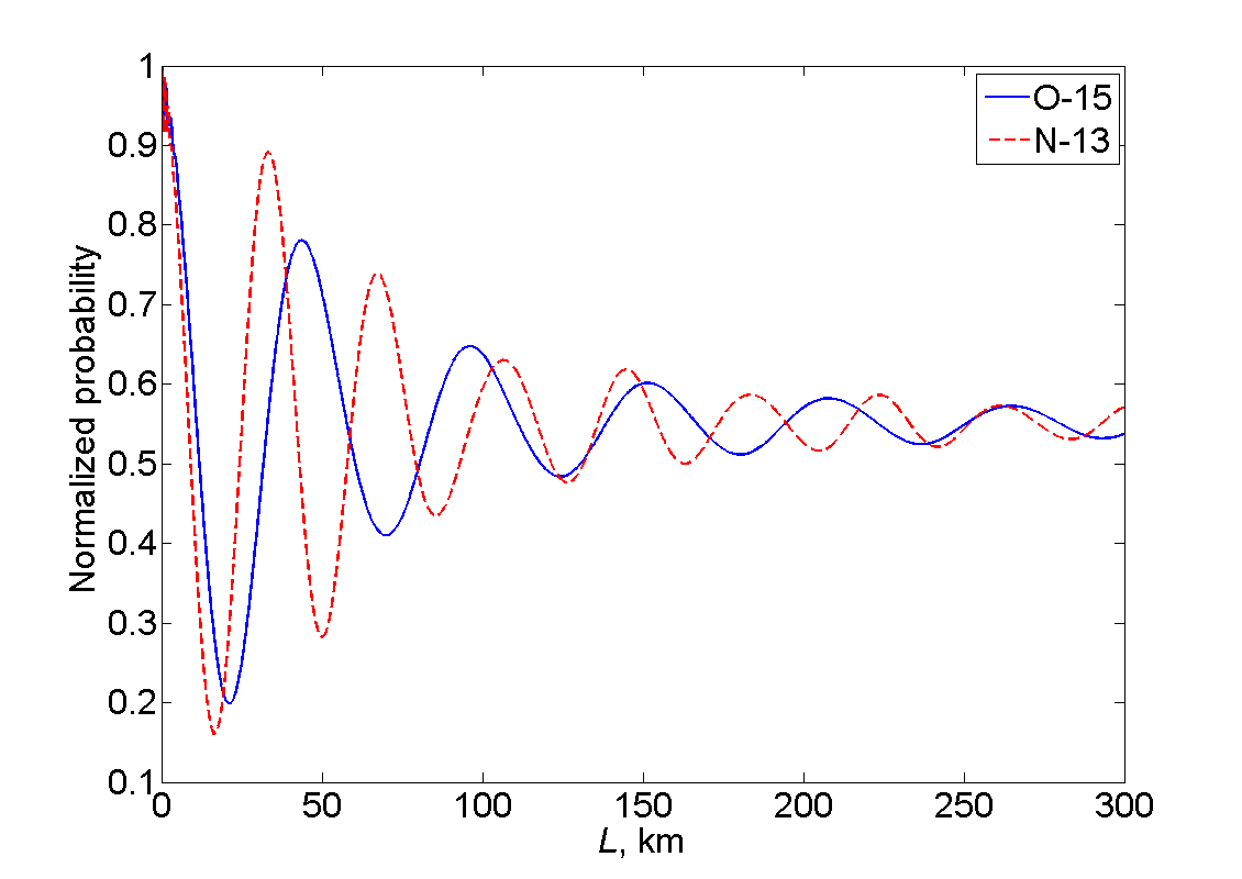
a) Distance $L$ from 0 to 300 km.

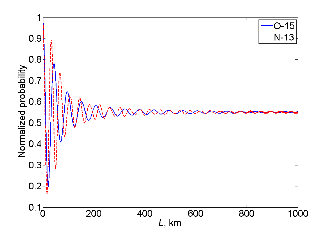
b) Distance $L$ from 0 to 1000 km.

Figure 4: Normalized probabilities of the neutrino oscillation processes with the neutrino production in the ${{}^{15}{\rm O}}$ and ${{}^{13}{\rm N}}$ decays and the registration by a Cl-Ar detector.

The coherence length for the ${{}^{13}{\rm N}}$ source turns out to be

$$L_{{\rm coh}}^{\textit{\rm N}}\approx 158{\rm\ km,}$$

which is larger than for the previously found ${{}^{15}{\rm O}}$ case (146 km) since the ${{}^{13}{\rm N}}$ source provides a more narrow neutrino momentum distribution.

Finally let us consider a more realistic combined source, where the neutrinos are produced in the ${{}^{15}{\rm O}}$ and ${{}^{13}{\rm N}}$ decays simultaneously. The registration is performed again by a chlorine-argon detector. When a neutrino is detected, one cannot distinguish, whether it came from a ${{}^{15}{\rm O}}$ or ${{}^{13}{\rm N}}$ nucleus. The calculations show that if the source is in the state of dynamic equilibrium, the probability of a neutrino being produced by a ${{}^{13}{\rm N}}$ decay is approximately 83% versus 17% for an ${{}^{15}{\rm O}}$ one. We will sum the probabilities for ${{}^{15}{\rm O}}$ and ${{}^{13}{\rm N}}$ given by formula (17) with different weights, and these probabilities of a neutrino being produced in one of two decays are one source of the weights.

Another source is as follows. Function (18) includes the constant $C$, which is different for our two cases. Let us introduce the notations $C_{\textit{\rm O}}$ and $C_{\textit{\rm N}}$ for the corresponding coefficients. In our approximation, these constants satisfy the relations

$$4\pi\int\limits_{0}^{\left|{\vec{p}}\right|_{\max}^{Z}}{C_{Z}\sqrt{\left({\left|{\vec{p}}\right|_{\max}^{Z}-\left|{\vec{p}}\right|}\right)\left({\left|{\vec{p}}\right|_{\max}^{Z}-\left|{\vec{p}}\right|+2m}\right)}\left({\left|{\vec{p}}\right|_{\max}^{Z}-\left|{\vec{p}}\right|+m}\right)\left|{\vec{p}}\right|^{2}d\left|{\vec{p}}\right|}=\frac{{{\mathop{1}\nolimits}}}{{\tau_{Z}}},$$ (21)

where the index $Z$ takes values “O” or “N” and $\tau_{Z}$ is the lifetime of the corresponding nucleus. Given that $\tau_{\textit{\rm O}}=122.24$ sec and $\tau_{\textit{\rm N}}=597.90$ sec, performing the numerical evaluation of the integral in (21), one finds the ratio of the coefficients to be ${{C_{\textit{\rm O}}}\mathord{\left/{\vphantom{{C_{\textit{\rm O}}}{C_{\textit{\rm N}}}}}\right.\kern-1.2pt}{C_{\textit{\rm N}}}}=1.0548$, which gives a small correction.

The resulting weights of probabilities (17) for the ${{}^{15}{\rm O}}$ and ${{}^{13}{\rm N}}$ nuclei are the products of the corresponding coefficients from these two sources. The weights can be chosen in a transparent way to be 0.1776 for the ${{}^{15}{\rm O}}$ contribution and 0.8224 for the ${{}^{13}{\rm N}}$ contribution. Total normalized function (18) for such an experiment is presented in Fig. 3 (dash-dotted line). The results of the numerical integration are depicted in Fig. 5.

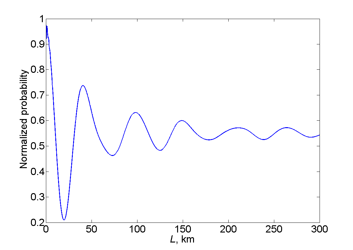
a) Distance $L$ from 0 to 300 km.

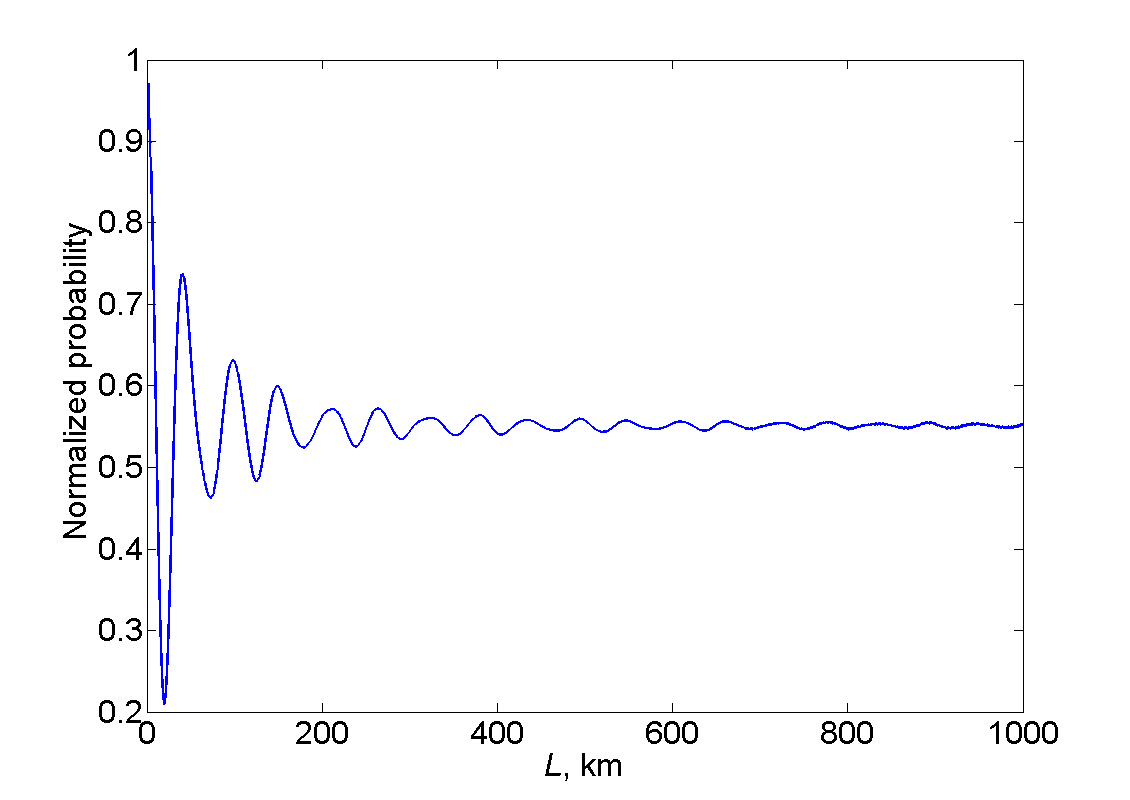
b) Distance $L$ from 0 to 1000 km.

Figure 5: Normalized probability of the neutrino oscillation process with the neutrino production in both the ${{}^{15}{\rm O}}$ and ${{}^{13}{\rm N}}$ decays simultaneously and the registration by a Cl-Ar detector.

The overlapping of the oscillation patterns from two different sources leads to an even more rapid fading out of the oscillations, and in this case the coherence length reads

$$L_{{\rm coh}}^{\textit{\rm O+N}}\approx 142{\rm\ km,}$$

which is less than for the ${{}^{15}{\rm O}}$ or ${{}^{13}{\rm N}}$ sources separately.

At the end of this section we would like to stress ones again that the coherence length discussed above differs essentially from the coherence length appearing in the standard quantum-mechanical description of neutrino oscillation in terms of wave packets. In the latter case the oscillation fading out and, consequently, the coherence length arises due to the quantum-mechanical uncertainty of neutrino momentum. In contrast to it, in the approach under consideration the neutrinos are supposed to have definite momenta (no momentum uncertainty), and the origin of the oscillation pattern blurring is the momentum distribution of the intermediate neutrinos. It is always present in a three-body decay, even if all the initial and final particles and nuclei have definite momenta. The above calculations show that this cause of oscillation fading out leads to much smaller coherence lengths than the ones, which are due to the natural momentum uncertainty considered in the standard approach. It means that the effect of neutrino non-monochromaticity taken into account in the framework of our approach is dominant in a realistic experimental setting, while the blurring due to the neutrino momentum uncertainty can be neglected compared to it.

3 Neutrino oscillations in experiments with detection in the charged-current interaction only

3.1 Theory

In the same way one can consider the neutrino oscillation process, where the neutrinos are produces in the charged-current interaction with nuclei and detected in both the charged- and neutral-current interactions with an electron. The process is described by the following diagrams:

             

The amplitude corresponding to diagram (23) should be summed over all the three neutrino mass eigenstates, i.e. $k=1,2,3$, as they all contribute. Since only the final electron is detected in the experiment, the probability of the process with $i$-th neutrino mass eigenstate in the final state should be summed over $i$ to give us the probability of registering an electron.

Now let us denote the particle momenta as follows: the momentum of the positron is $q$, the momentum of the virtual neutrinos is $p_{\rm n}$, the momentum of the outgoing electron is $k$, the momentum of the incoming electron is $k_{1}$, the momentum of the outgoing neutrino is $k_{2}$, the momentum of the initial nucleus is $P^{(1)}=\left({E^{(1)},\vec{P}^{(1)}}\right)$ and the momentum of the final nucleus is $P^{(1^{\prime})}=\left({E^{(1^{\prime})},\vec{P}^{(1^{\prime})}}\right)$ (we retain the notations of the previous section for the nuclear values in order to use the formulas from it without redefinitions).

Again we use the approximation of Fermi’s interaction and take the time-dependent propagator (6) keeping the neutrino masses only in the exponential. The amplitude corresponding to diagram (22) in the momentum representation, when $y^{0}-x^{0}=T$, looks like

$$M_{\rm nc}^{(i)} = i\frac{{G_{\rm F}^{\,2}}}{4p_{\rm n}^{0}}\,{U_{1i}^{*}}e^{-i\frac{{m_{i}^{2}-p_{\rm n}^{2}}}{{2{p^{0}_{\rm n}}}}T}\,\bar{\nu}_{i}\left(k_{2}\right)\gamma^{\mu}\left({1-\gamma^{5}}\right)\hat{p}_{\rm n}\gamma^{\rho}\left({1-\gamma^{5}}\right)v\left(q\right)j_{\rho}^{(1)}\left({P^{(1)},P^{(1^{\prime})}}\right)\times$$

$$\times\left[\left(-\frac{1}{2}+\sin^{2}\theta_{\rm W}\right)\bar{u}\left(k\right)\gamma_{\mu}(1-\gamma^{5})u\left(k_{1}\right)+\sin^{2}\theta_{\rm W}\bar{u}\left(k\right)\gamma_{\mu}(1+\gamma^{5})u\left(k_{1}\right)\right].$$

Similarly, the amplitude corresponding to diagram (23) summed over $k$ reads

$$M_{\rm cc}^{(i)} = -i\frac{{G_{\rm F}^{\,2}}}{4{p_{\rm n}^{0}}}\,{U_{1i}^{*}}\left(\sum\limits_{k=1}^{3}{\left|{U_{1k}}\right|^{2}}e^{-i\frac{{m_{i}^{2}-p_{\rm n}^{2}}}{{2{p^{0}_{\rm n}}}}T}\right)\bar{u}\left(k\right)\gamma^{\mu}(1-\gamma^{5})\hat{p}_{\rm n}\gamma^{\rho}\left({1-\gamma^{5}}\right)v\left(q\right)\times$$ (25)

$$\times j_{\rho}^{(1)}\left({P^{(1)},P^{(1^{\prime})}}\right)\bar{\nu}_{i}\left(k_{2}\right)\gamma_{\mu}(1-\gamma^{5})u\left(k_{1}\right).$$

The squared modulus of the total amplitude $M_{\rm tot}^{(i)}=M_{\rm nc}^{(i)}+M_{\rm cc}^{(i)}$, averaged with respect and summed over particles’ polarizations, factorizes in the approximation $p_{\rm n}^{2}=0$ as follows:

$$\left\langle{\left|M_{\rm tot}^{(i)}\right|^{2}}\right\rangle=\left\langle{\left|M_{1}\right|^{2}}\right\rangle\left\langle{\left|M_{2}^{(i)}\right|^{2}}\right\rangle\frac{{1}}{{4(p_{\rm n}^{0})^{2}}}.$$ (26)

Here $\left\langle{\left|M_{1}\right|^{2}}\right\rangle$ is given by (9),

$$\left\langle{\left|M_{2}^{(i)}\right|^{2}}\right\rangle = 64G_{\rm F}^{\,2}\left[\left|B_{i}+A_{i}\left(-\frac{1}{2}+\sin^{2}\theta_{\rm W}\right)\right|^{2}(p_{\rm n}k_{1})^{2}+\left|A_{i}\right|^{2}\sin^{4}\theta_{\rm W}(p_{\rm n}k)^{2}-\right.$$ (27)

$$-\sin^{2}\theta_{\rm W}\,{\rm Re}\left(\left(B_{i}+A_{i}\left(-\frac{1}{2}+\sin^{2}\theta_{\rm W}\right)\right)A_{i}^{*}\right)(p_{\rm n}k_{2})m^{2}\Bigg{]},$$

where the notations

$$A_{i}={U_{1i}^{*}}e^{-i\frac{{m_{i}^{2}-p_{\rm n}^{2}}}{{2{p^{0}_{\rm n}}}}T},\quad B_{i}={U_{1i}^{*}}\left(\sum\limits_{k=1}^{3}{\left|{U_{1k}}\right|^{2}}e^{-i\frac{{m_{i}^{2}-p_{\rm n}^{2}}}{{2{p^{0}_{\rm n}}}}T}\right)$$ (28)

are introduced.

Following the outlined procedure, we introduce the virtual neutrino 4-momentum $p$ in the same manner, multiply the squared amplitude (26) by the delta function of energy-momentum conservation $(2\pi)^{4}\delta(P^{(1)}+k_{1}-P^{(1^{\prime})}-q-k-k_{2})$, substitute $p$ instead of $p_{\rm n}$, multiply by $2\pi\delta(P^{(1)}-P^{(1^{\prime})}-q-p)$ and integrate the result with respect to the phase volume of the final particles and nucleus. Next we sum the resulting differential probability of the process over the final neutrino type $i$, substitute $T={{Lp^{0}}\mathord{\left/{\vphantom{{Lp^{0}}{\left|{\vec{p}}\right|}}}\right.\kern-1.2pt}{\left|{\vec{p}}\right|}}$, multiply the result by $\left|{\vec{p}}\right|^{2}$ and integrate it with respect to $\left|{\vec{p}}\right|$ from $\left|{\vec{p}}\right|_{\min}$ to $\left|{\vec{p}}\right|_{\max}$. We arrive at the probability of detecting an electron:

$$\frac{{dW}}{{d\Omega}}=\int\limits_{\left|{\vec{p}}\right|_{\min}}^{\left|{\vec{p}}\right|_{\max}}{\frac{{d^{3}W}}{{d^{3}p}}\left|{\vec{p}}\right|^{2}d\left|{\vec{p}}\right|}=\int\limits_{\left|{\vec{p}}\right|_{\min}}^{\left|{\vec{p}}\right|_{\max}}{\frac{{d^{3}W_{1}}}{{d^{3}p}}W_{2}\left|{\vec{p}}\right|^{2}d\left|{\vec{p}}\right|}.$$ (29)

Here $\frac{{d^{3}W}}{{d^{3}p}}$ is the differential probability of the whole process, where the intermediate neutrinos have a definite momentum $\vec{p}$ and the final neutrino mass eigenstate is of any type, $\frac{{d^{3}W_{1}}}{{d^{3}p}}$ is the differential probability of decay of the initial nucleus into the final nucleus, a positron and a massless fermion with the momentum $\vec{p}$ given by (13) and

$$W_{2} = \frac{1}{{2p^{0}2k_{1}^{0}}}\int{\frac{{d^{3}k}}{{\left({2\pi}\right)^{3}2k^{0}}}\frac{{d^{3}k_{2}}}{{\left({2\pi}\right)^{3}2k_{2}^{0}}}\sum\limits_{i=1}^{3}{\left.{\left\langle{\left|{M_{2}^{(i)}}\right|^{2}}\right\rangle}\right|_{\scriptstyle p_{\rm n}=p\hfill\atop\scriptstyle T={{Lp^{0}}\mathord{\left/{\vphantom{{Lp^{0}}{\left|{\vec{p}}\right|}}}\right.\kern-1.2pt}{\left|{\vec{p}}\right|}}\hfill}}\left({2\pi}\right)^{4}\delta\left({k_{1}+p-k-k_{2}}\right)}=$$ (30)

$$= \frac{{G_{\rm F}^{2}m}}{{2\pi}}\frac{{2\left|{\vec{p}}\right|^{2}}}{{2\left|{\vec{p}}\right|+m}}\left[{1-2\sin^{2}\theta_{\rm W}\left({1+\frac{{2\left|{\vec{p}}\right|}}{{2\left|{\vec{p}}\right|+m}}}\right)+4\sin^{4}\theta_{\rm W}\left({1+\frac{1}{3}\left({\frac{{2\left|{\vec{p}}\right|}}{{2\left|{\vec{p}}\right|+m}}}\right)^{2}}\right)+}\right.$$

$$\left.{+4\sin^{2}\theta_{\rm W}\left({1+\frac{{2\left|{\vec{p}}\right|}}{{2\left|{\vec{p}}\right|+m}}}\right)P_{ee}\left(L\right)}\right]$$

is the probability of the neutrino scattering in the detector. Now we will use expression (29) to consider several examples.

3.2 Specific examples

In the present subsection we consider neutrino oscillation experiments, where the neutrinos are produced in the decays of ${{}^{15}{\rm O}}$ or ${{}^{13}{\rm N}}$ and registered by a water-based Cherenkov detector. For simplicity we assume that the final electron is detected, when its speed exceeds the speed of light in water. It gives us the registration threshold $\left|{\vec{p}}\right|_{\min}^{\textit{\rm Cher}}=775{\ \rm keV}$.

Neglecting the dependence of the nuclear form-factors on the momentum transfer, we can again approximate the differential probability of neutrino production by the function

$$\frac{{d^{3}W_{1}}}{{d^{3}p}}=C\sqrt{\left({\left|{\vec{p}}\right|_{\max}-\left|{\vec{p}}\right|}\right)\left({\left|{\vec{p}}\right|_{\max}-\left|{\vec{p}}\right|+2m}\right)}\left({\left|{\vec{p}}\right|_{\max}-\left|{\vec{p}}\right|+m}\right).$$ (31)

The normalized distribution functions $\frac{{d^{3}W_{1}}}{{d^{3}p}}W_{2}$ at the point $L=0$ in this approximation are represented in Fig. 6 (solid and dashed lines).

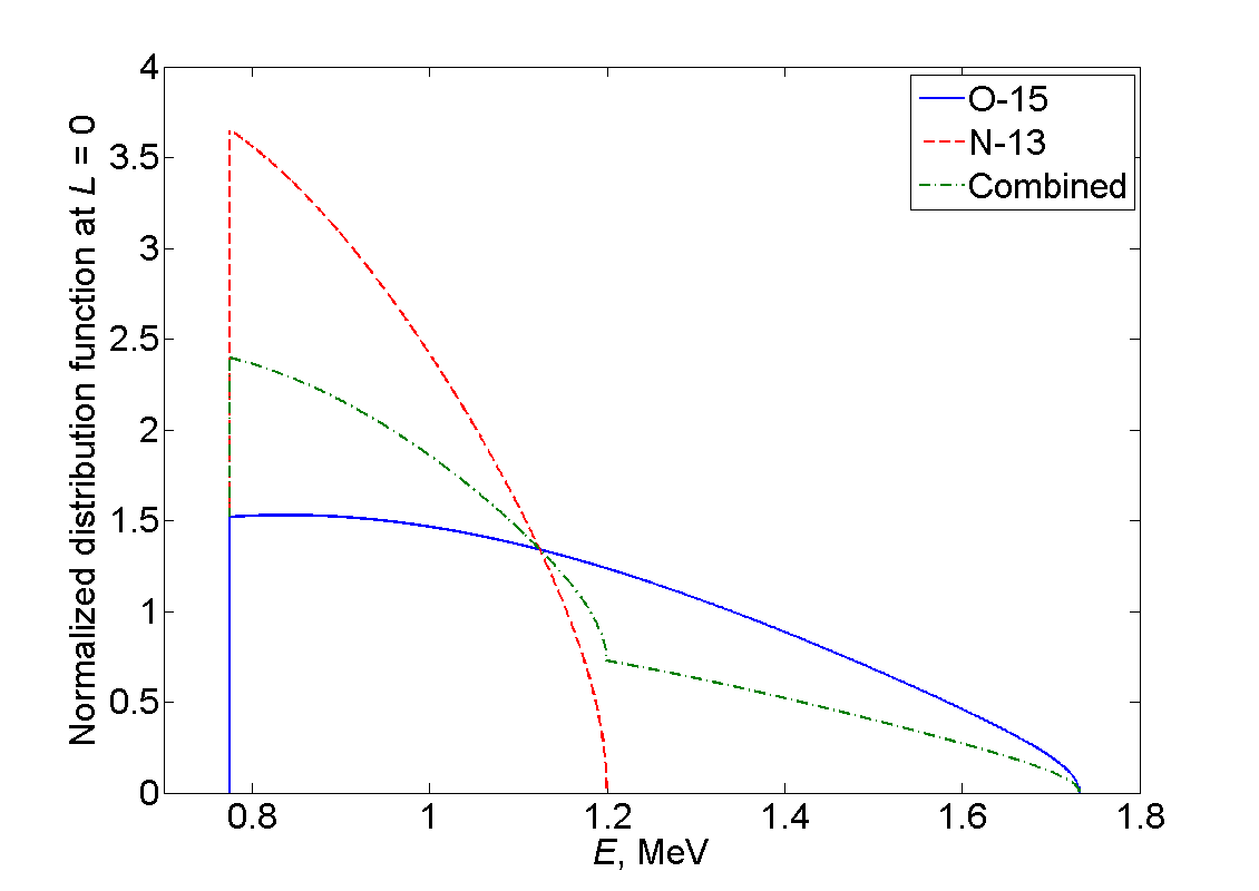
Figure 6: Normalized distribution functions $\frac{{d^{3}W_{1}}}{{d^{3}p}}W_{2}$ at the point $L=0$ for ${{}^{15}{\rm O}}$, ${{}^{13}{\rm N}}$ and combined sources and a water-based Cherenkov detector.

The results of numerical integration with the same parameters as were used in the previous section are depicted in Fig. 7.

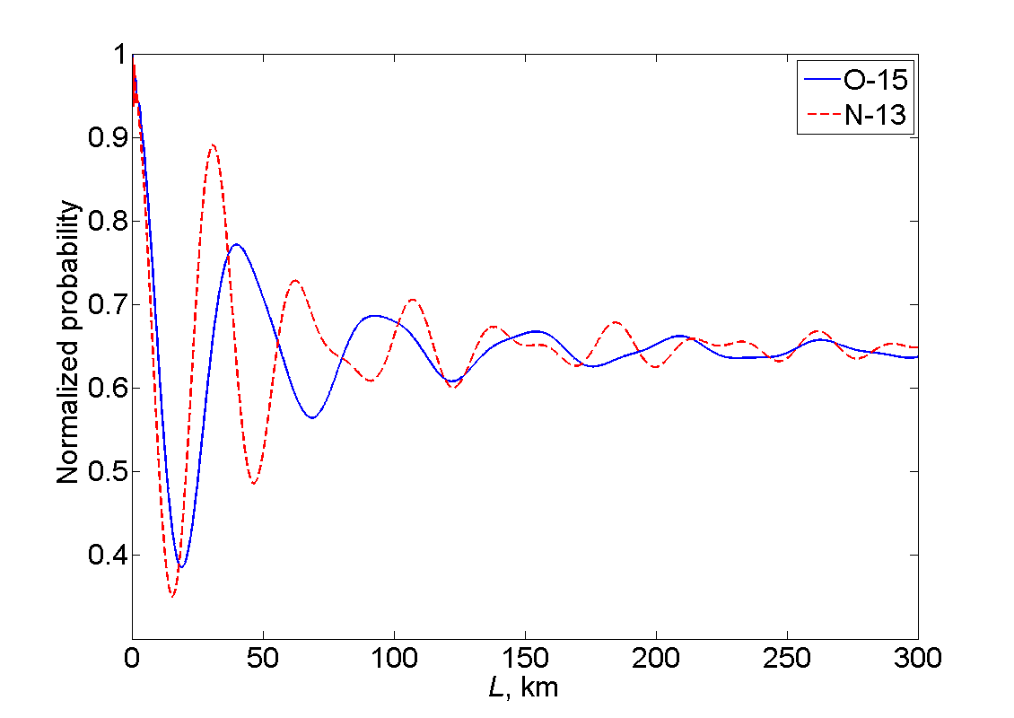
a) Distance $L$ from 0 to 300 km.

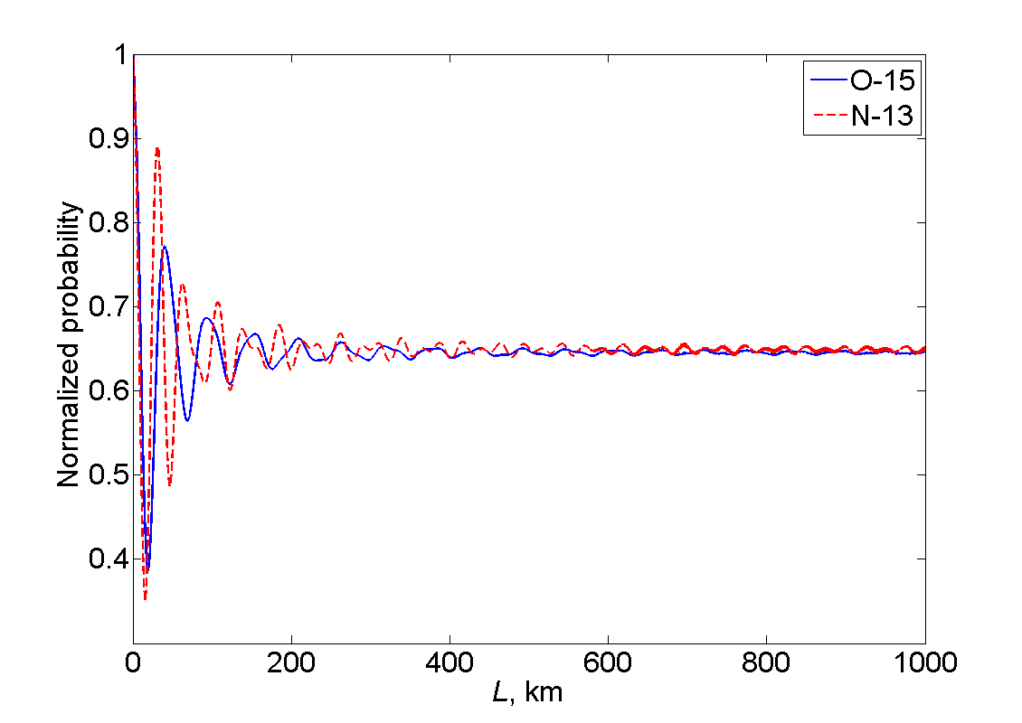
b) Distance $L$ from 0 to 1000 km.

Figure 7: Normalized probabilities of the neutrino oscillation processes with the neutrino production in the ${{}^{15}{\rm O}}$ and ${{}^{13}{\rm N}}$ decays and the registration by a water-based Cherenkov detector.

The irregular form of the oscillation pattern in this case is due to the sharp cut of the neutrino momentum distribution, defined by the detection threshold. The coherence lengths here turn out to be

$$L_{{\rm coh}}^{\textit{\rm O}}\approx 80{\rm\ km},\quad L_{{\rm coh}}^{\textit{\rm N}}\approx 75{\rm\ km.}$$

Finally let us consider the combined ${{}^{15}{\rm O}}$ and ${{}^{13}{\rm N}}$ source. The summation of the probabilities is performed with the same weights as it was discussed in the previous section. The normalized distribution function $\frac{{d^{3}W_{1}}}{{d^{3}p}}W_{2}$ at the point $L=0$ for this case is shown in Fig. 6 (dash-dotted line). The results of numerical integration are presented in Fig. 8.

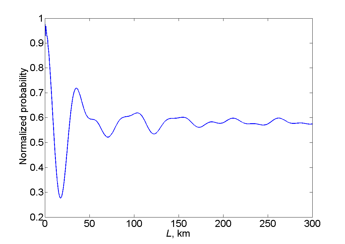
a) Distance $L$ from 0 to 300 km.

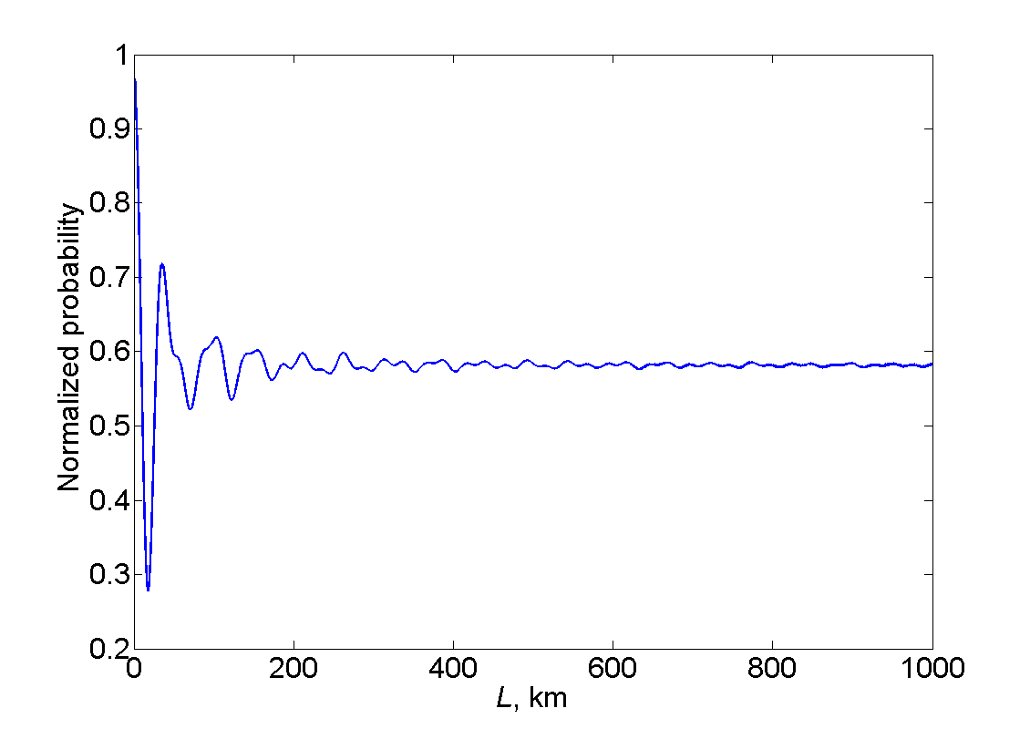
b) Distance $L$ from 0 to 1000 km.

Figure 8: Normalized probability of the neutrino oscillation process with the neutrino production in both the ${{}^{15}{\rm O}}$ and ${{}^{13}{\rm N}}$ decays simultaneously and the registration by a water-based Cherenkov detector.

The coherence length reads

$$L_{{\rm coh}}^{\textit{\rm O+N}}\approx 32{\rm\ km,}$$

which is, as expected, less than for the ${{}^{15}{\rm O}}$ and ${{}^{13}{\rm N}}$ sources separately.

We would like to note here that, unlike the case of registration only in the charged-current interaction, discussed in Section 2, the asymptotic values of the normalized probabilities of the neutrino oscillation processes presented in Figs. 7, 8 are all different. This is due to the fact that, in the case of registration in the charged-current interaction only, the oscillating expression $P_{ee}\left(L\right)$, given by (15), factorizes. Thus, the oscillation asymptotic behavior is determined by the average of $P_{ee}\left(L\right)$. However, when the registration is performed in both the charged- and neutral-current interactions, there is no such factorization, as one can see from formulas (29)–(30). The numerical evaluation gives that in the case of ${{}^{15}{\rm O}}$ and ${{}^{13}{\rm N}}$ sources separately the asymptotic values are close to each other and read 0.6454 and 0.6489, respectively, whereas in the case of combined source the asymptotic value is 0.5818.

4 Conclusion

A novel quantum field-theoretical approach to the description of neutrino oscillation processes passing at finite space-time intervals is discussed. It is based on the Feynman diagram technique in the coordinate representation supplemented by modified rules of passing to the momentum representation, which reflect the experimental situation at hand. Wave packets are not employed, we use only the description in terms of plane waves, which considerably simplifies the calculations. The neutrino flavor states turn out to be unnecessary and only the neutrino mass eigenstates are used.

We have explicitly shown that the approach allows one to consistently describe the processes of neutrino oscillations. The predictions for the probabilities of these processes are found to completely coincide with the results obtained in the standard quantum-mechanical approach.

The approach under consideration also predicts a suppression of neutrino oscillations with distance. In the standard quantum-mechanical description this suppression is assumed to arise due to the quantum uncertainty of neutrino momentum. However, in a realistic experiment there is also another source of the suppression effect. It is the intermediate neutrino being non-monochromatic, which always takes place in the case of a tree-body decay even if all the involved particles are assumed to have definite momenta. If the production process has a two-particle final state, the momentum spread of the neutrinos comes from the momentum spread of the initial particles and/or nuclei. In any realistic experimental situation a neutrino momentum distribution of this type is always present and is determined by the spectral characteristics of the production and detection processes. The width of this distribution is much larger than that of the natural neutrino momentum distribution due to the quantum-mechanical uncertainty, considered in the standard approach. Consequently, the corresponding coherence length turns out to be much smaller than the one predicted in the standard quantum-mechanical approach, and hence the former coherence length is dominant in experiments. The decoherence process caused by the neutrino momentum quantum uncertainty also affects the oscillation pattern blurring, but we can neglect it compared to the more powerful effect due to the momentum spread of the intermediate neutrinos.

In the approach under consideration neutrino oscillation is an interference process, and the coherence length is found by analogy with interference of non-monochromatic light in optics with the help of the visibility function. It is completely defined by the production and detection processes and cannot be decomposed into coherence lengths for pairs of neutrino mass eigenstates. The coherence lengths for five combinations of production and detection processes have been explicitly calculated. It was found that the coherence length in the experiments with two production processes is smaller than the coherence length in experiments with only one of the production processes and with the same detection process.

It is necessary to mention that, in the developed approach, there is no analogue of the localization term, which appears in the wave-packet treatment of neutrino oscillations. This is due to the fact that the approach under consideration is based on the assumption that the sizes of the neutrino source and detector are much smaller than the distance between them, which is always fulfilled in neutrino oscillation experiments. Since the coherence length is of the order of the latter distance, this means that the production and detection processes are localized in space-time regions much smaller than the oscillation length. In the standard approach this is exactly the condition that the localization term does not suppress the oscillations.

Finally we would like to note that the advantages of the discussed approach are physical clearness and technical simplicity.

References

- [1] A. Pais and O. Piccioni, Phys. Rev. 100 (1955) 1487.
- [2] B. Pontecorvo, Sov. Phys. JETP 6 (1957) 429.
- [3] V. N. Gribov and B. Pontecorvo, Phys. Lett. B 28 (1969) 493.
- [4] R. , Springer Tracts Mod. Phys. 153 (1999) 1.
- [5] C. Giunti and C. W. Kim, “Fundamentals of Neutrino Physics and Astrophysics,” Oxford, UK: Univ. Pr. (2007).
- [6] S. Bilenky, Lect. Notes Phys. 817 (2010) 1.
- [7] K. Nakamura and S. T. Petcov, in: M. Tanabashi et al. [Particle Data Group], Phys. Rev. D 98 (2018) no.3, 030001.
- [8] C. Giunti, C. W. Kim, J. A. Lee and U. W. Lee, Phys. Rev. D 48 (1993) 4310.
- [9] W. Grimus and P. Stockinger, Phys. Rev. D 54 (1996) 3414.
- [10] M. Beuthe, Phys. Rept. 375 (2003) 105 [hep-ph/0109119].
- [11] A. G. Cohen, S. L. Glashow and Z. Ligeti, Phys. Lett. B 678 (2009) 191 [arXiv:0810.4602 [hep-ph]].
- [12] A. E. Lobanov, Annals Phys. 403 (2019) 82 [arXiv:1507.01256 [hep-ph]].
- [13] R. P. Feynman, Phys. Rev. 76 (1949) 749.
- [14] R. P. Feynman, Phys. Rev. 76 (1949) 769.
- [15] I. P. Volobuev, Int. J. Mod. Phys. A 33 (2018) no.13, 1850075 [arXiv:1703.08070 [hep-ph]].
- [16] V. O. Egorov and I. P. Volobuev, Phys. Rev. D 97 (2018) no.9, 093002 [arXiv:1709.09915 [hep-ph]].
- [17] V. O. Egorov and I. P. Volobuev, arXiv:1712.04335 [hep-ph].
- [18] N. N. Bogoliubov and D. V. Shirkov, “Introduction to the theory of quantized fields,” 3d edition, New York, Chichester, Brisbane, Toronto: John Wiley & Sons (1980).
- [19] E. Byckling and K. Kajantie, “Particle Kinematics,” London, New York, Sydney, Toronto: John Wiley & Sons (1973).
- [20] A. Bohr and B. R. Mottelson, “Nuclear Structure: Volume I: Single-Particle Motion,” World Scientific (1998).
- [21] M. Tanabashi et al. [Particle Data Group], Phys. Rev. D 98 (2018) no.3, 030001.