Abstract

Ice flow velocities close to the terminus of major outlet glaciers of the Greenland Ice Sheet can vary on the time scale of years to hours. Such flow speed variations can be explained as the reaction to changes in terminus geometry with help of a 3D full-Stokes ice flow model. Starting from an initial steady state geometry, parts of an initially 7 km long floating terminus are removed. Flow velocity increases everywhere up to 4 km upstream of the grounding line, and complete removal of the floating terminus leads to a doubling of flow speed. The model results conclusively show that the observed velocity variations of outlet glaciers is dominated by the terminus geometry. Since terminus geometry is mainly controlled by calving processes and melting under the floating portion, changing ocean conditions most probably have triggered the recent geometry and velocity variations of Greenland outlet glaciers.

1 Introduction

Flow velocities close to the terminus of major outlet Glaciers of the Greenland Ice Sheet can vary substantially on the time scale of years (e.g. Rignot and Kanagaratnam,, 2006), and to a lesser degree seasonally (Joughin et al.,, 2008), and episodically during calving events (Amundson et al.,, 2008; Nettles et al.,, 2008). Several major Greenland Ice Sheet outlet glaciers accelerated within the last decade (Joughin et al.,, 2004), sometimes to double their pre-acceleration velocity within three years, occasionally followed by a slowdown in the following years (Howat et al.,, 2007). The dynamic changes of these outlet glaciers control the short term evolution of the ice sheet geometry, and their changing calving flux impacts the ice sheet mass budget, and therefore sea level.

The close timing of the acceleration of Helheim and Kangerdlussuaq Glaciers on the east coast (Howat et al.,, 2007) and Jakobshavn Isbræ on the west coast (Joughin et al.,, 2004) hints to an external forcing not related to internal dynamic instabilities of the outlet glacier system. The obvious possible causes are atmospheric forcing through high meltwater production that affects basal motion (e.g. Zwally et al.,, 2002), or the influence of ocean temperature on terminus melt rate, and therefore the geometry of the calving front (Holland et al.,, 2008). Increased meltwater production can supply important amounts of water to the ice-bedrock interface by hydro-fracturing (Van der Veen,, 1998; Das et al.,, 2008), temporarily increasing the already very high water pressure under the ice sheet in vicinity of the ice stream (Lüthi et al.,, 2002). Due to stress transfer from the ice stream trunk to its surroundings (Truffer and Echelmeyer,, 2003; Lüthi et al.,, 2003), stream velocities are susceptible to changes in basal motion in the surrounding ice sheet, and could be affected by higher sliding velocities there. If on the other hand increased heat flux from the ocean is the driver, thinning of the floating terminus and higher calving rates would be expected, as were indeed observed at Jakobshavn Isbræ (Thomas et al.,, 2003; Holland et al.,, 2008).

In this contribution we use a three-dimensional full-Stokes ice flow model to investigate the relation between terminus geometry and ice flow velocity. The model results show that the velocity at the grounding line is controlled by the length of a floating terminus, even in absence of friction at pinning points. Removing a floating terminus part by part leads to step-wise increases in flow velocity, similar to what has been observed at Jakobshavn Isbræ (Amundson et al.,, 2008) and Helheim Glacier (Nettles et al.,, 2008).

2 Flow model

The FISMO Full Ice Stream Model was used to investigate the effect of changing geometry on flow velocities. The finite element code FISMO solves the Stokes equations for slow, incompressible flow with variable viscosity, expressed in terms of the field variables velocity $\mathbf{v}$ and pressure $p$

$$-\nabla p+\eta\,\nabla^{2}\mathbf{v}+2\,\mathbf{D}\cdot\nabla\eta+\rho\mathbf{g} =\mathbf{0}\,,$$ (1a)

$$\mathrm{tr}\mathbf{D}=\nabla\mathbf{v} =0\,,$$ (1b)

where $\mathbf{D}=\frac{1}{2}\left(\nabla\mathbf{v}+(\nabla\mathbf{v})^{T}\right)$ is the Cauchy strain rate tensor. The viscosity $\eta$ of glacier ice is strain rate dependent and is calculated according to Glen’s flow law (a power-law rheology) as

$$\mathbf{D}=A\,\tau^{n-1}\,\mbox{\boldmath$\sigma$\unboldmath}^{d}\qquad\Longleftrightarrow\qquad\eta=\frac{1}{2}\,A^{-\frac{1}{n}}\,II_{\mathbf{D}}{}^{\frac{1-n}{n}}\,.$$ (2)

where $\mbox{\boldmath$\sigma$\unboldmath}^{d}$ is the deviatoric stress tensor, $II_{\mbox{\boldmath$\sigma$\unboldmath}^{d}}=\left(\frac{1}{2}\sigma^{d}_{ij}\sigma^{d}_{ij}\right)^{\frac{1}{2}}$ and $II_{\mathbf{D}}=\left(\frac{1}{2}D_{ij}D_{ij}\right)^{\frac{1}{2}}$ the the second invariants of $\mbox{\boldmath$\sigma$\unboldmath}^{d}$ and $\mathbf{D}$, $A=215\,\mathrm{MPa}^{-3}\,\mathrm{a}^{-1}$ is the rate factor commonly assumed for temperate ice (Paterson,, 1999), and $n=3$. To avoid inifinte viscosity at vanishing strain rates, a small constant $\epsilon=1\cdot 10^{-6}\,\mathrm{a}^{-1}$ was added to $II_{\mathbf{D}}$.

Velocity was prescribed as Dirichlet boundary condition on the parts of the domain representing bedrock. On the parts of the boundary in contact with air a zero stress boundary condition was applied (which in the Galerkin finite element method employed requires no effort). On the faces in contact with the ocean, normal stress was set equal to the hydrostatic water pressure $\sigma_{n}=-\rho_{\mathrm{water}}gz$ (ocean level is assumed at $z=0$). To limit the geometrical extent of the model, a stress boundary condition was prescribed on the boundaries to the inland ice, with the normal stress equal to ice overburden pressure $\sigma_{n}=-\rho_{\mathrm{ice}}g(z_{s}-z)$ (the minus sign indicates a compressive force). The latter boundary condition has been tested to work well for an infinite inclined slab of ice, and is useful since it does not force ice flow into the computational domain.

Equations (1) and (2) together with the boundary conditions were solved numerically with the FISMO finite element (FE) code, which builds on the Libmesh FE-library (Kirk, 2007) that uses the PETSc parallel solver library. To obtain a numerically stable and divergence-free velocity solution, Q2Q1 isoparametric Taylor-Hood Elements on 27-node hexahedra were used. In Libmesh all boundary conditions are enforced with a penalty method.

The nonlinear equation system arising from Equation (2) was solved with a fixed-point iteration. An ALE (arbitrary Lagrange-Euler) formulation was used in an explicit time stepping scheme for the evolution of the model geometry. Given the velocity $\mathbf{v}$ from the previous time step, vertical mesh node positions $z$ at the free boundaries (surface and floating terminus) are updated during the time step $\Delta t$ according to

$$\Delta z=\left(\left(\mathbf{v}\cdot\mathbf{n}\right)_{z}+b\right)\Delta t$$ (3)

where $\mathbf{n}$ is the face normal, index $z$ indicates the vertical component, and $b$ is the annual net balance, i.e. the amount of ice added or removed during a year at the surface or under the floating terminus. The time step $\Delta t$ was chosen so that the maximum vertical displacement was $1\,\mathrm{m}$. After each time step, all mesh nodes were adjusted to their initial relative positions between surface and bedrock.

3 Model setup

The bedrock is parametrized as a fjord geometry that resembles Jakobshavn Isbræ. The grounding line location is fixed at $x=0$, ice is grounded in the domain $x>0$ and floating for $x<0$. Bedrock elevation $z_{b}(x,y)$ is assumed to be $z_{b}=0$ outside of a straight channel geometry that is parametrized in the domain $x>0$ by

$$z_{c}(x) =\begin{cases}1+\beta_{r}(x_{r}-x)\,,&x<x_{r}\\ 1\,,&x_{r}\leq x<x_{t}\\ e^{-(\beta_{t}(x_{t}-x))^{2}},&x\geq x_{t}\\ \end{cases}$$

$$z_{b}(x,y) =-z_{c}(x)\,e^{-(\mu y)^{2}}\,H_{m}$$ (4)

where $z_{c}(x)$ is the unit centerline depth of the channel and $\mu$ determines the cross-sectional shape of the channel. The position $x_{t}$ determines where the channel reaches is maximum depth and $x_{r}$ is the position from where on the channel starts raising towards the calving front (parameters are given in Table 1). The initial ice surface was parametrized with

$$z_{s}(x)=\begin{cases}50+4.5\sqrt{x}\,,&x\geq 0\,,\\ 50\,,&x<0\,.\end{cases}$$ (5)

For the initial bottom elevation of the floating terminus the bedrock geometry given in Equation (3) was extended. The geometry of the ice surface and the floating terminus was evolved until it became stationary. This resulted in surface draw-down in the main ice stream channel where longitudinal extension rates are highest.

The usually complicated polythermal structure of polar ice streams is neglected and all ice is assumed to be at the melting point. This assumption includes the important effect on ice dynamics of a thick layer of temperate ice close to the base, the thickness of which is at least $300\,\mathrm{m}$ at Jakobshavn Isbræ (Iken et al.,, 1993; Lüthi et al.,, 2002) and might even amount to $700\,\mathrm{m}$ (Lüthi et al.,, 2008). Such an approach underestimates the stress transfer to the surrounding ice sheet through the kilometer-thick layer of very cold ice close to the surface (Truffer and Echelmeyer,, 2003; Lüthi et al.,, 2003).

Velocity at the ice-bedrock contact is set to zero and basal motion is therefore ignored. This assumption is not realistic, but reasonable for the task of investigating the importance of geometry change on flow velocities. Moreover, the flow of Jakobshavn Isbræ, for example, seems not to be dominated by basal motion, and high flow velocities are thought to be largely due to a thick layer of temperate ice and the steep surface slope.

The geometry was discretized with hexahedra elements (the central part of the mesh is shown in Figure 1). Since the domain is symmetric about the $x$-$z$-plane, only one half of the geometry has to be meshed, and the boundary condition on the $x$-$z$-plane is $v_{y}=0$. The computational mesh of the grounded ice consists of 25x20 elements in the horizontal, and 10 elements in the vertical. The floating terminus was discretized with up to 30x11x10 elements, depending on terminus length. Element sizes are reduced in $x$-direction around the calving front where velocity gradients are biggest.

The annual net mass balance at the surface is assumed to be elevation dependent with $b(z)=\gamma(z-z_{\mathrm{ELA}})$ with a mass balance gradient $\gamma=0.005\,\mathrm{a}^{-1}$ and an equilibrium line altitude $z_{\mathrm{ELA}}=1100\,\mathrm{m}$, which is the order of measured values close to the ice sheet margin at Jakobshavn Isbræ. Net mass balance under the floating terminus was set to $-50\,\mathrm{m}\,\mathrm{a}^{-1}$.

The model experiment was started with an initial geometry as described above, and with a floating terminus of $7\,\mathrm{km}$ length. The elevation of the surface and the bottom of the floating terminus were allowed to evolve until they reached a stationary state.

4 Model results

To investigate the influence of the length of the floating terminus on the stress state and the flow velocities, parts from the front of the floating terminus were removed. New velocity solutions were calculated without any further evolution of the geometry. The geometries with terminus lengths of 7, 2, 1 and $0\,\mathrm{km}$ are plotted in Figure 1 next to the corresponding centerline velocities. Flow velocities increase with shorter terminus length, and nearly double at the grounding line when the floating terminus is completely removed.

The characteristic local maximum of flow velocity around the grounding line (black and blue curves in Fig. 1) is due to changing surface slopes in a small over-deepening plotted in the top panel of Figure 1. The ice is up to $5\,\mathrm{m}$ below hydrostatic equilibrium at the grounding line (top plot of Fig. 1) and reaches equilibrium at about four ice thicknesses along the floating terminus. A similar surface depression close to the calving front has been found in other modeling studies (e.g. Lestringant,, 1994).

The removal of the floating terminus induces changes in the stress state at the grounding line, as shown in Figures 2 and 3. Longitudinal deviatoric stress, which determines the rate of longitudinal extension, changes from negative (compressive) to positive (extensive) at the grounding line when the floating terminus is removed. Also the mean stress (plotted in Fig. 3b as the deviation from overburden pressure) shows a marked change with reversed slope and a kink at the water line (red lines in Fig. 3).

5 Discussion

The length and shape of the floating terminus controls the size and distribution of glacier flow velocity in vicinity of the grounding line, as is illustrated in Figure 1. There is a striking similarity of the modeled velocities along the centerline of our prototype outlet glacier with the measured evolution of terminus velocities at Jakobshavn Isbræ (Figure 2 in Joughin et al.,, 2004). Characteristic features like the maximum of flow velocity at the grounding line are also visible in the modeled velocities. The major difference between model and reality is the measured increase in flow velocity up to $40\,\mathrm{km}$ upstream of the grounding line, while our model experiment only shows a speedup in the last $4\,\mathrm{km}$ upstream of the grounding line. The difference is due to the model experiment setup that did not evolve the surfce after removal of the floating terminus, which corresponds to rapid disintegration of the floating ice. The flow acceleration would migrate inland together with the surface drawdown, as was exemplified in model studies of Pine Island Glacier (Antarctica) (Schmeltz et al.,, 2002; Payne et al.,, 2004). In these studies the removal of the terminus immediately influenced ice flow far inland due to very weak coupling to the bed over large parts of the glacier. In contrast, we assumed full coupling, which affects flow velocity only within 5 ice thicknesses from the grounding line.

Ice shelf buttressing is usually assumed to result from frictional forces acting on the floating terminus or ice shelf at pinning points, or at its sides (e.g. Dupont and Alley,, 2005). In the absence of friction on the terminus the total resistive horizontal force in flow direction is that of water pressure acting as a normal stress on the interface between ice and ocean. The integral of this normal stress over the interface area, weighted by the face normal, is constant and independent of the length and shape, presence or absence of the terminus. In the presence of a floating terminus the horizontal compressive force is evenly distributed over the cross section at the grounding line (Fig. 3). In the absence of the terminus the water pressure acts only below the water line, which leads to extensive deviatoric stresses with a maximum at the water line, and corresponding high extensional ice deformation rates there. The geometry of compact floating ice in contact with grounded ice has a major influence on the stress distribution in the grounding line area. The model results presented above show that ice shelf buttressing is mainly an effect of the geometry of floating portion.

Since the flow velocity is sensitive to terminus geometry, a growing floating terminus leads to slower flow velocities. This effect might explain the observation that Jakobshavn Isbræ slows in winter when a compact floating portion forms in the terminus area (Joughin et al.,, 2008).

The cause for big changes of terminus geometry, and therefore flow velocity, is most likely the influence of increased heat flux from the ocean causing increased melt under the floating portion of the terminus. For Jakobshavn Isbræ  a strong increase of ocean bottom temperature has been measured, the influence of which coincides with thinning of the floating terminus and flow acceleration (Holland et al.,, 2008). Alternatively, changes of the calving process by ponding meltwater in crevasses could explain the disintegration of floating termini (Benn et al.,, 2007), although observations of increase of such ponding water have not been made for the Greenland outlet glaciers discussed above.

6 Conclusions

The geometry of the terminus area is the dominant control on the velocity field close to the grounding line of an outlet glacier. Short term geometry changes, such as the disintegration of a floating terminus, calving, or the creation of embayments in grounded ice, greatly affects the flow field close to the terminus.

A typical calving event at big outlet glaciers such as Jakobshavn Isbræ removes up to $400\,\mathrm{m}$ of ice from the glacier terminus. Measurements have shown that the glacier velocity reacts immediately (within a 15 minute measurement interval), but no extra movement could be observed during calving events (Amundson et al.,, 2008; Nettles et al.,, 2008). Such almost step-wise increase in flow velocity can be reproduced with a 3D flow model, when parts of a floating terminus are removed. Short term flow velocity variations thus are mainly an effect of stress redistribution, which in turn is controlled by changes of the terminus geometry.

Table 1: Parameters for the ice stream geometry

maximum channel depth	$H_{m}$	1600	m b.s.l.
location of deepest point	$x_{t}$	15	km
location of bed inflexion	$x_{r}$	7	km
steepness of trough on centerline	$\beta_{t}$	2	$10^{-4}$
centerline slope	$\beta_{r}$	-8	$10^{-5}$
steepness of sides	$\mu$	7	$10^{-4}$

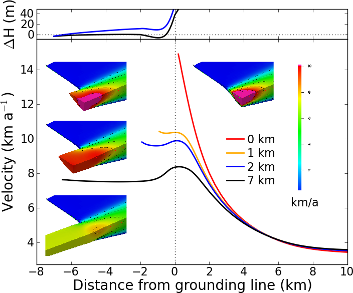
Figure 1: Modeled centerline flow velocity at the surface for the terminus geometries shown next to the curves. Decreasing the length of the floating terminus affects the value and spatial distribution of flow velocities. Grounding line position is indicated with a vertical dotted line. Top panel: surface elevation (blue, displayed $40\,\mathrm{m}$ lower) and height above buoyancy (black).

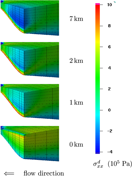
Figure 2: Modeled deviatoric stress $\sigma_{xx}^{d}$ in flow direction at the grounding line. The model geometry is sliced along the centerline, and at the grounding line (i.e. the terminus is not shown). Terminus lengths are 7, 2, 1 km, and no terminus.

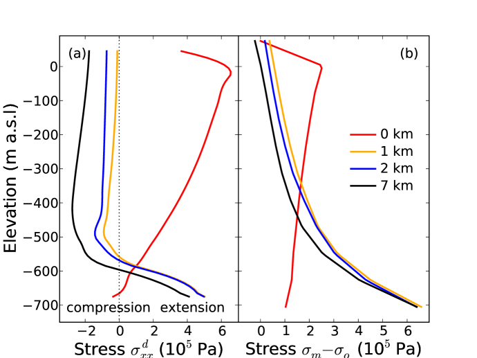
Figure 3: (a) Modeled deviatoric component of longitudinal stress $\sigma_{xx}^{d}$ in a vertical profile $20\,\mathrm{m}$ upstream of the grounding line. (b) Deviation of the mean stress $\sigma_{m}$ with respect to the hydrostatic overburden stress $\sigma_{o}$.

References

- Amundson et al., (2008) Amundson, J., Truffer, M., Lüthi, M. P., Fahnestock, M., Motyka, R. J., and West, M. (2008). Glacier, fjord, and seismic response to recent large calving events, Jakobshavn Isbræ, Greenland. Geophysical Research Letters, 35:L22501. doi:10.1029/2008GL035281.
- Benn et al., (2007) Benn, D. I., Warren, C. R., and Mottram, R. H. (2007). Calving processes and the dynamics of calving glaciers. Earth-Science Reviews, 82:143–179.
- Das et al., (2008) Das, S. B., Joughin, I., Behn, M. D., Howat, I. M., King, M. A., Lizarralde, D., and Bhatia, M. P. (2008). Fracture propagation to the base of the Greenland Ice Sheet during supraglacial lake drainage. Science, 320. doi: 10.1126/science.1153360.
- Dupont and Alley, (2005) Dupont, T. and Alley, R. (2005). Assessment of the importance of ice-shelf buttressing to ice-sheet flow. Geophysical Research Letters, 32:L04503.
- Holland et al., (2008) Holland, D. M., Thomas, R. H., de Young, B., Ribergaard, M. H., and Lyberth, B. (2008). Acceleration of Jakobshavn Isbræ triggered by warm subsurface ocean waters. Nature Geoscience.
- Howat et al., (2007) Howat, I. M., Joughin, I., and Scambos, T. A. (2007). Rapid changes in ice discharge from Greenland outlet glaciers. Science, 315:1559–1561.
- Iken et al., (1993) Iken, A., Echelmeyer, K., Harrison, W. D., and Funk, M. (1993). Mechanisms of fast flow in Jakobshavns Isbrae, Greenland, Part I: Measurements of temperature and water level in deep boreholes. Journal of Glaciology, 39(131):15–25.
- Joughin et al., (2008) Joughin, I., Howat, I. M., Fahnestock, M., Smith, B., Krabill, W., Alley, R. B., Stern, H., , and Truffer, M. (2008). Continued evolution of Jakobshavn Isbrae following its rapid speedup. Journal of Geophysical Research, 113:F04006. doi:10.1029/2008JF001023.
- Joughin et al., (2004) Joughin, I. R., Abdalati, W., and Fahnestock, M. A. (2004). Large fluctuations in speed on Greenland’s Jakobshavn Isbræ glacier. Nature, 432:608–610.
- Lestringant, (1994) Lestringant, R. (1994). A two-dimensional finite-element study of flow in teh transition zone between an ice sheet and an ice shelf. Annals of Glaciology, 20:67–72.
- Lüthi et al., (2003) Lüthi, M., Funk, M., and Iken, A. (2003). Indication of active overthrust faulting along the Holocene-Wisconsin transition in the marginal zone of Jakobshavn Isbræ. Journal of Geophysical Research, 108(B11). doi:10.1029/2003JB002505.
- Lüthi et al., (2002) Lüthi, M., Funk, M., Iken, A., Gogineni, S., and Truffer, M. (2002). Mechanisms of fast flow in Jakobshavns Isbrae, Greenland; Part III: measurements of ice deformation, temperature and cross-borehole conductivity in boreholes to the bedrock. Journal of Glaciology, 48(162):369–385.
- Lüthi et al., (2008) Lüthi, M. P., Fahnestock, M., and Truffer, M. (2008). Observational evidence for a thick temperate layer at the base of Jakobshavn Isbræ. Journal of Glaciology. (submitted).
- Nettles et al., (2008) Nettles, M., Larsen, T. B., Elesegui, P., Hamilton, G. S., Stearns, L. A., Ahlstrom, A. P., Davis, J. L., Andersen, M. L., de Juan, J., Khan, S. A., Stenseng, L., Ekstrom, G., and Forsberg, R. (2008). Step-wise changes in glacier flow speed coincide with calving and glacial earthquakes at Helheim Glacier, Greenland. Geophysical Research Letters.
- Paterson, (1999) Paterson, W. S. B. (1999). The Physics of Glaciers. Butterworth-Heinemann, third edition.
- Payne et al., (2004) Payne, A. J., Vieli, A., Shepherd, A. P., Wingham, D. J., and Rignot, E. (2004). Recent dramatic thinning of largest West Antarctic ice stream triggered by oceans. Geophysical Research Letters, 31:L23401. doi:10.1029/2004GL021284.
- Rignot and Kanagaratnam, (2006) Rignot, E. and Kanagaratnam, P. (2006). Changes in the velocity structure of the Greenland Ice Sheet. Science, 311:986–990. doi:10.1126/science.1121381.
- Schmeltz et al., (2002) Schmeltz, M., Rignot, E., Dupont, T. K., and MacAyeal, D. R. (2002). Sensitivity of pine island glacier, west antarctica, to changes in ice-shelf and basal conditions: a model study. Journal of Glaciology, 48(163):552–558.
- Thomas et al., (2003) Thomas, R. H., Abdalati, W., Frederick, E., Krabill, W. B., Manizade, S., and Steffen, K. (2003). Investigation of surface melting and dynamic thinning on jakobshavn isbrae, greenland. Journal of Glaciology, 49(165):231–239.
- Truffer and Echelmeyer, (2003) Truffer, M. and Echelmeyer, K. (2003). Of Isbræ and Ice Streams. Annals of Glaciology, 36:66–72.
- Van der Veen, (1998) Van der Veen, C. J. (1998). Fracture mechanics approach to penetration of surface crevasses on glaciers. Cold Regions Science and Technology, 27(1):31–47.
- Zwally et al., (2002) Zwally, H. J., Abdalati, W., Herring, T., Larson, K., Saba, J., and Steffen, K. (2002). Surface melt-induced acceleration of Greenland ice-sheet flow. Science, 297(5579):218–222.