Asymmetric sending or not-sending twin-field quantum key distribution in practice

Abstract

Quantum key distribution (QKD) offers a secret way to share keys between legitimate users which is guaranteed by the law of quantum mechanics. Most recently, the limitation of transmission distance without quantum repeaters was broken through by twin-field QKD [Nature (London) 557, 400 (2018)]. Based on its main idea, sending or not-sending (SNS) QKD protocol was proposed [Phys. Rev. A 98, 062323 (2018)], which filled the remaining security loopholes and can tolerate large misalignment errors. In this paper, we give a more general model for SNS QKD, where the two legitimate users, Alice and Bob, can possess asymmetric quantum channels. By applying the method present in the work, the legitimate users can achieve dramatically increased key generation rate and transmission distance compared with utilizing the original symmetric protocol. Therefore, our present work represents a further step along the progress of practical QKD.

PACS number(s): 03.67.Dd, 03.67.Hk,42.65.Lm

I Introduction

Quantum key distribution (QKD), based on the law of quantum mechanicsHK ; PShor ; DMayers , allows two distant users (Alice and Bob) to establish a string of secure keys despite at the existence of the malicious eavesdropper (Eve). Since the first QKD protocol BB84 BB84 came into being, numerous protocols DecoyH ; DecoyW ; DecoyL ; Side ; MDI were proposed to promote its development. The goal of QKD is to own high security and long transmission distance simultaneously. To illuminate the relationship between transmittance ($\eta$) and key rate ($R$), $R=-\log(1-\eta)$ is summarized PLOB without quantum repeaters, which are regarded as a solution to overcome the limit of $R\propto O(\eta)$. However, due to the restriction of current technology, quantum repeater is far from use QM1 ; QM2 . Luckily, twin-field (TF) QKD, based on the single-photon interference, with $R\propto O(\sqrt{\eta})$ is presented TF .

TF-QKD inherits the idea of measurement-device independent (MDI) and drastically improves the transmission distance at the same time. Upon its proposal, TF-QKD has been extensively studied TFCui ; TFLin ; TFWang ; TFTamaki ; TFYin ; TFYu ; TFMa ; TFCurty . Among these works, Wang et al. developed a sending or not-sending (SNS) TF-QKD protocolTFWang . Without phase announcement for Z basis (signal state), SNS TF-QKD fills the remaining loophole of original TF-QKD. Moreover, due to single-photon interferences only in X basis (decoy states), SNS TF-QKD can tolerate the largest misalignment errors. This protocol seems much more practical for implementations than the original TF-QKD, and its performance has been investigated by considering statistical fluctuation and finite numbers of phase slices TFYu .

In real life, most locations of users are not on the symmetry of untrusted third party (UTP). Especially in a multi-user network, UTP can hardly locate at the centre of all users. One simple solution is to add extra fibers or attenuations at the closer side to compensate the difference between the two transmittances, where original symmetric protocol is certainly suitable. This seems to be a ”$buckets\;effect$”, and the final key rate is limited by the smaller transmittance.

In this work, we develop a general model for the SNS TF-QKD, where the two parties possess asymmetric quantum channels. Different from previous works on asymmetric MDI-QKD AsyXu ; AsyHu ; AsyWang , decoy-state method can not applied directly in asymmetric SNS TF-QKD. According to our analysis, decoy-state method still can be an efficient and secure method in present work only by satisfying some extra constraints.

The paper is organized as follow: In Sec II, we will introduce some basic steps on how to implement asymmetric SNS TF-QKD. Besides, decoy-state method and other theoretical models are given. Corresponding numerical simulations are shown in Sec III. Finally, summaries and outlooks are given out in Sec IV.

II The Decoy-State Asymmetric SNS TF-QKD

In this section, without adding extra compensation of transmittance, we will show the possibility of applying decoy state asymmetric SNS TF-QKD only by adjusting dependent intensities and other parameters.

II.1 Basic steps of decoy-state asymmetric SNS TF-QKD

Below let us describe the detailed SNS TF-QKD in asymmetric situation. Corresponding schematic setup is shown in Fig.1.

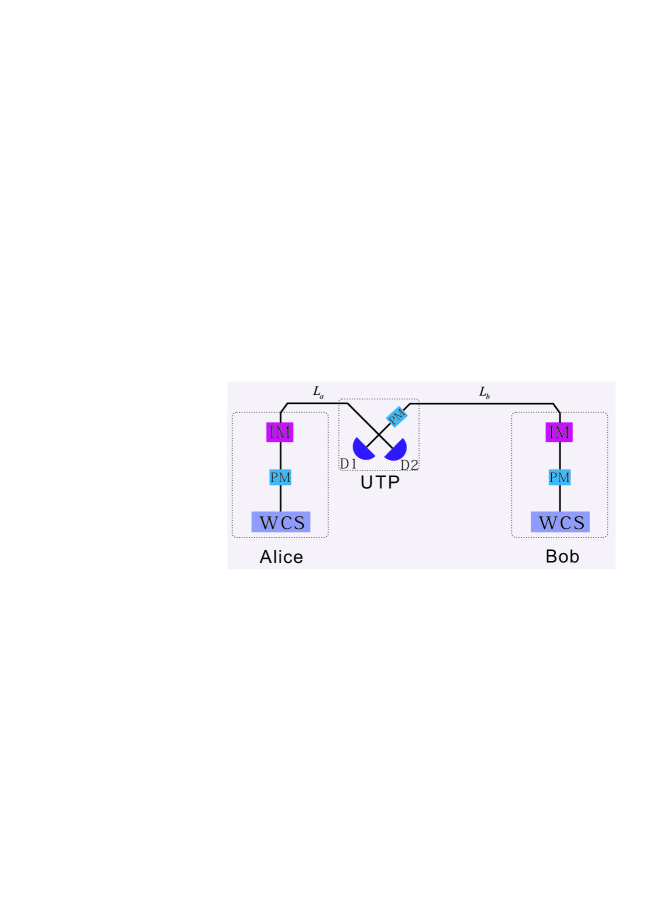
Figure 1: Schematic setup of asymmetric SNS TF-QKD. WCS: weak coherent source; PM: phase modulator; IM: intensity modulator; D1(D2): single-photon detector. Bob is farther from UTP than Alice; $L_{a}$ and $L_{b}$ are the distance between user and the UTP respectively.

(0) For each time window, $i$, Alice and Bob send a strong reference light with coherent state pulses to the UTP. Besides, they add extra random phases ${\delta_{a}}$ and ${\delta_{b}}$ to their pulses. Here, we denote the distance between user and the UTP as $L_{a}$ and $L_{b}$ ($L_{a}<L_{b}$ ) respectively.

(1) Alice (Bob) randomly chooses signal window (Z-window) and decoy window (X-window) with probability ${P_{za}}$ (${P_{zb}}$) and ${1-P_{za}}$ (${1-P_{zb}}$). In Z-window, Alice (Bob) determines to send a signal state pulse $\left|{\sqrt{{u_{a}}}{e^{i{\delta_{a}}+i{\gamma_{a}}}}}\right\rangle$ ($\left|{\sqrt{{u_{b}}}{e^{i{\delta_{b}}+i{\gamma_{b}}}}}\right\rangle$) with probability ${\varepsilon_{a}}$ (${\varepsilon_{b}}$), and not to send with $1-{\varepsilon_{a}}$ $(1-{\varepsilon_{b}})$; In X-window, Alice and Bob emit decoy state pulse $\left|{\sqrt{\alpha}{e^{i{\delta_{a}}+i{\gamma_{a}}}}}\right\rangle$and $\left|{\sqrt{{\beta}}{e^{i{\delta_{b}}+i{\gamma_{b}}}}}\right\rangle$, respectively. ${{\alpha}}\in\{{v_{a}},{w_{a}},o\}$; ${{\beta}}\in\{{v_{b}},{w_{b}},o\}$. ${\gamma_{a}}$ and ${\gamma_{b}}$ are the global phase. Note that, in asymmetric situation, Alice is reasonably assumed to be closer to the UTP than Bob. Then, she should postpone the emission for $\tau$ time-windows to ensure the synchronization, i.e, the two states chosen at the same time-windows reach the beam splitter simultaneously.

(2) After the UTP performs the phase compensation with the aid of strong reference light, the two-mode state turns into, for example, $\left|{\sqrt{{\alpha}}{e^{i{\delta_{a}}}}}\right\rangle\left|{\sqrt{{\beta}}{e^{i{\delta_{b}}}}}\right\rangle$. Then the UTP measures the incoming pulses and records the clicking or non-clicking events of the two detectors.

(3)The UTP announces the measurement outcomes after the distribution progress ends. Then, the users announce for each pulse whether it is a Z-window or an X-window. The intensity and extra phase of X-window should also be public. An efficient event is defined as the following two cases: (a) Alice and Bob both choose Z-windows and only one detector clicking at UTP’s side. In this case, four events and the corresponding raw keys are shown in Table 1; (b) Alice and Bob both choose the corresponding intensities in X-window when UTP announces single clicking of detectors, and the phases ${\delta_{a}}$ , ${\delta_{b}}$ should satisfy either of following two inequations:

$$\left|{{\delta_{a}}-{\delta_{b}}}\right|\leq\frac{{2\pi}}{M},\qquad\left|{{\delta_{a}}-{\delta_{b}}-\pi}\right|\leq\frac{{2\pi}}{M}.$$ (1)

$M$ is the number of phase slices pre-determine by users.

Table 1: When an effective event happened in Z-window, if Alice (Bob) decides to send a signal pulse, she (he) records a bit 1 (0); if Alice (Bob) decides not to send a signal pulse, she (he) records a bit 0 (1);

	Sending	Not-sending
Sending	10	11
Not-sending	00	01

(4)After the announcement, Alice and Bob get the gain in Z-window. By sacrificing some bits in Z-window, Alice and Bob get the average quantum bit error rate (QBER) in Z basis. Besides, they estimate the single-photon yield $Y_{1}$ and the error rate $e_{1}$ by observed values in X-window.

(5)Error correction and privacy amplification are performed before calculating the final secret keys.

II.2 Decoy-state method and theoretical models

Before introducing the decoy-state formulae of this protocol, we will review its essence. In a decoy-state method DecoyH ; DecoyW ; DecoyL , legitimate users need to modulate light pulses into different intensities and post-announce the details. Eve can not distinguish which one is the signal state pulse, and can only carry out identical attacking strategies in quantum channels. As a result, the photon-number-splitting attacks will affect the yields, $Y_{n}$, and QBER, $e_{n}$ which only depend on the numbers of photons $n$. Whether an eavesdropper exists can be judged from the reasonability of $Y_{n}$ and $e_{n}$. In essence, decoy state method is based on the following equations:

$${Y_{n}}(signal)={Y_{n}}(decoy),$$

$${e_{n}}(signal)={e_{n}}(decoy).$$ (2)

Now let us come to the asymmetric SNS TF-QKD: Denote Alice and Bob send pulses with intensities $x_{a},x_{b}$ respectively, and corresponding transmittances are ${\eta_{a}},{\eta_{b}}$ $({\eta_{a}}>{\eta_{b}})$. For simplicity, we assume that the two detectors at UTP’s sides are identical and each with a dark count rate $P_{d}$ and detection efficiency ${\eta_{d}}$ individually.

The counting rate of the n-photon states which causes effective events can be written as:

$$Q_{n}^{{x_{a}}{x_{b}}}=\sum\limits_{m=0}^{n}{\frac{{{e^{-{x_{a}}}}{x_{a}}^{m}}}{{m!}}}\frac{{{e^{-{x_{b}}}}{x_{b}}^{n-m}}}{{(n-m)!}}[1-{(1-{P_{d}})^{2}}{(1-{\eta_{a}})^{m}}{(1-{\eta_{b}})^{n-m}}].$$ (3)

Hereafter, we call the above event as the n-photon effective event. Considering it may possess $m$ photons from Alice and ($n-m$) photons form Bob, the equivalent photon number distribution can be formulated as:

$${P_{n}}({x_{a}}+{x_{b}})=\sum\limits_{m=0}^{n}{\frac{{{e^{-{x_{a}}}}{x_{a}}^{m}}}{{m!}}}\frac{{{e^{-{x_{b}}}}{x_{b}}^{n-m}}}{{(n-m)!}}.$$ (4)

Correspondingly, the equivalent yield of the n-photon effective event can be expressed as:

$$Y_{n}^{{x_{a}}{x_{b}}}= \frac{{Q_{n}^{{x_{a}}{x_{b}}}}}{{{P_{n}}({x_{a}}+{x_{b}})}}$$

$$= 1-{(1-{P_{d}})^{2}}{[\frac{{{x_{a}}(1-{\eta_{a}})+{x_{b}}(1-{\eta_{b}})}}{{{x_{a}}+{x_{b}}}}]^{n}}$$

$$= 1-{(1-{P_{d}})^{2}}{[\frac{{k(1-{\eta_{a}})+(1-{\eta_{b}})}}{{k+1}}]^{n}},$$ (5)

where $k=\frac{{{x_{a}}}}{{{x_{b}}}}$. Obviously, in the asymmetric case, the value of $Y_{n}^{{x_{a}}{x_{b}}}$ is not only dependent on the photon numbers ($n$), but also related to the ratio ($k$) of two intensities. Therefore, the original lower bound of the single-photon counting rate ($Y_{1}$) and upper bound of the single-photon error rate ($e_{1}$) cannot be applied directly. In the Appendix, we will give corresponding proof for the renewed formulae.

In Eq.(II.2), $Y_{n}^{{x_{a}}{x_{b}}}$ is concerned with the ratio $k$. For convenience, we denote $Y_{n}^{{x_{a}}{x_{b}}}$ ($Q_{n}^{{x_{a}}{x_{b}}}$)as $Y_{n}^{k}$ ($Q_{n}^{k}$); Denote ${w_{a}}+{w_{b}}={\mu_{1}},{v_{a}}+{v_{b}}={\mu_{2}},\frac{{{w_{a}}}}{{{w_{b}}}}={k_{1}},\frac{{{v_{a}}}}{{{v_{b}}}}={k_{2}}.$ According to the analysis in the Appendix, for ${k_{1}}\leq{k_{2}}$, we can get the lower bound of single-photon yield in X-window

$$Y_{1}^{L}=\frac{{{P_{2}}({\mu_{2}}){Q_{{\mu_{1}}}}-{P_{2}}({\mu_{1}}){Q_{{\mu_{2}}}}+[{P_{2}}({\mu_{1}}){P_{0}}({\mu_{2}})-{P_{2}}({\mu_{2}}){P_{0}}({\mu_{1}})]{Y_{0}}}}{{{P_{2}}({\mu_{2}}){P_{1}}({\mu_{1}})-{P_{2}}({\mu_{1}}){P_{1}}({\mu_{2}})}}.$$ (6)

In addition, to estimate the single-photon yield in Z-window, a restriction on the ratio of intensities, e.g., $\frac{{{u_{1}}}}{{{u_{2}}}}\geq{k_{1}}$, should be imposed. In this case, the yield in X-window is not larger than the yield in Z-window. Thus, $Y_{1}^{L}$ can also be looked as the lower bound in Z-window. Accordingly, the QBER of single-photon pulses is given by TFWang :

$${e_{1}}\leq e_{1}^{U}=\frac{{{Q_{{\mu_{1}}}}{E_{{\mu_{1}}}}-{P_{0}}({\mu_{1}}){Y_{0}}{e_{0}}}}{{{P_{1}}({\mu_{1}}){Y_{1}^{L}}}},$$ (7)

where ${e_{0}}=0.5$.

In real-life implementations, the average counting rate and QBER in X-window can be directly measured. In this work, we use a linear model to predict what it should be observed in experiment. Consider a two-mode state $\left|{\sqrt{{\alpha}}{e^{i{\delta_{a}}}}}\right\rangle\left|{\sqrt{{\beta}}{e^{i{\delta_{b}}}}}\right\rangle$ goes through the quantum channels and a beam-splitter. It turns into $\left|{\sqrt{\frac{{\alpha{\eta_{a}}}}{2}}{e^{i{\delta_{a}}}}+\sqrt{\frac{{\beta{\eta_{b}}}}{2}}{e^{i{\delta_{b}}}}}\right\rangle\otimes\left|{\sqrt{\frac{{\alpha{\eta_{a}}}}{2}}{e^{i{\delta_{a}}}}-\sqrt{\frac{{\beta{\eta_{b}}}}{2}}{e^{i{\delta_{b}}}}}\right\rangle$. The corresponding gains ($Q_{\alpha\beta}^{{\delta_{a}}{\delta_{b}}}$) and the quantum-bit errors ($Q_{\alpha\beta}^{{\delta_{a}}{\delta_{b}}}E_{\alpha\beta}^{{\delta_{a}}{\delta_{b}}}$) are given by

$$Q_{\alpha\beta}^{{\delta_{a}}{\delta_{b}}}=(1-{P_{d}}){e^{-\frac{{\alpha{\eta_{a}}}}{2}-\frac{{\beta{\eta_{b}}}}{2}}}({e^{-\cos({\delta_{a}}-{\delta_{b}})\sqrt{\alpha\beta{\eta_{a}}{\eta_{b}}}}}+{e^{\cos({\delta_{a}}-{\delta_{b}})\sqrt{\alpha\beta{\eta_{a}}{\eta_{b}}}}})-2{(1-{P_{d}})^{2}}{e^{-\alpha{\eta_{a}}-\beta{\eta_{b}}}},$$ (8)

$$Q_{\alpha\beta}^{{\delta_{a}}{\delta_{b}}}E_{\alpha\beta}^{{\delta_{a}}{\delta_{b}}}=(1-{P_{d}}){e^{-\frac{{\alpha{\eta_{a}}}}{2}-\frac{{\beta{\eta_{b}}}}{2}-\cos({\delta_{a}}-{\delta_{b}})\sqrt{\alpha\beta{\eta_{a}}{\eta_{b}}}}}-{(1-{P_{d}})^{2}}{e^{-\alpha{\eta_{a}}-\beta{\eta_{b}}}}.$$ (9)

After phase post-selection in X-window, $|{\delta_{a}}-{\delta_{b}}|$ are ranging among $[0,\frac{{2\pi}}{M}]\cup[\pi,\pi+\frac{{2\pi}}{M}]$. Define the system error rate as ${E_{sys}}=\frac{1}{2}-\frac{{\sqrt{{x_{1}}{\eta_{1}}{x_{2}}{\eta_{2}}}}}{{{x_{1}}{\eta_{1}}+{x_{2}}{\eta_{2}}}}+\frac{{2\sqrt{{x_{1}}{\eta_{1}}{x_{2}}{\eta_{2}}}}}{{{x_{1}}{\eta_{1}}+{x_{2}}{\eta_{2}}}}{E_{d}}$, where ${E_{d}}$ is the build-in misalignment error of the optical system. Here ${E_{sys}}$ comes from single-photon interference and leads to an extra equivalent phase differences between Alice and Bob, denoted as $\Delta=\arccos(1-2{E_{sys}})$. By integrating, the average gain and quantum-bit errors can be expressed as

$${Q_{\alpha\beta}}=\frac{{{M^{2}}}}{{4{\pi^{2}}}}\int_{\Delta}^{\frac{{2\pi}}{M}+\Delta}{\int_{0}^{\frac{{2\pi}}{M}}{Q_{\alpha\beta}^{{\delta_{a}}{\delta_{b}}}d{\delta_{a}}}}d{\delta_{b}},$$ (10)

$${Q_{\alpha\beta}}{E_{\alpha\beta}}=\frac{{{M^{2}}}}{{4{\pi^{2}}}}\int_{\Delta}^{\frac{{2\pi}}{M}+\Delta}{\int_{0}^{\frac{{2\pi}}{M}}{Q_{\alpha\beta}^{{\delta_{a}}{\delta_{b}}}E_{\alpha\beta}^{{\delta_{a}}{\delta_{b}}}d{\delta_{a}}}}d{\delta_{b}}.$$ (11)

Finally, with the above formulae, the key generation rate can be expressed as

$$R={P_{za}}{P_{zb}}\{[{\varepsilon_{a}}(1-{\varepsilon_{b}}){e^{-{u_{a}}}}{u_{a}}+{\varepsilon_{b}}(1-{\varepsilon_{a}}){e^{-{u_{b}}}}{u_{b}}]Y_{1}^{L}[1-H(e_{1}^{U})]-{Q_{{u_{a}}{u_{b}}}}fH({E_{{u_{a}}{u_{b}}}})\},$$ (12)

where ${Q_{{u_{a}}{u_{b}}}}$ and ${E_{{u_{a}}{u_{b}}}}$ are the average gain and QBER of effective events in Z-window;$f$ is the error correction efficiency; $H(\xi)=-\xi{\log_{2}}(\xi)-(1-\xi){\log_{2}}(1-\xi)$.

III Numerical simulations

With all the above formulae, we can now carry out numerical simulations for the asymmetric SNS TF-QKD. To be noted, for the asymmetric case, in order to reach the highest visibility of single-photon interference in the UTP’s side, certain constraints should be set on the system parameters, to make light from each path possessing the same intensity before the beam-splitter. Statistical fluctuation is also taken into account. For simplicity, we make a Gaussian distribution assumption of the channel fluctuations and apply the standard deviation method, setting the failure probability as $10^{-7}$ yu2 . Finite number of phase slices, $M$, is considered. The experimental parameters used here are taken from Ref.TFYu , which are listed out in Table 2. Besides, global optimization is applied for a better performance.

Table 2: Parameters for simulations. $\eta_{d}$ and $P_{d}$ are detection efficiency and dark counting rate per pulse of UTP’s detectors respectively; $E_{d}$ is misalignment error of optical system; $\alpha$ is the transmission fiber loss constant; $f$ is the error correction efficiency; $N$ is the number of total pluses.

$\eta_{d}$	$P_{d}$	$E_{d}$	$\alpha(dB/km)$	$f$	$N$
50%	$1\times 10^{-10}$	15%	0.2	1.1	$10^{12}$

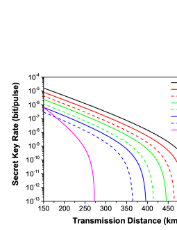
Figure 2: Result of secret key rate with respect to the total transmission distance ($L_{a}+L_{b}$). The line marked with ’0’ represents the original symmetric case; ’$La=0$’ represents the special case that Alice and UPT are together. Among the rest lines, Label ’$Asy$’ means the asymmetric method in this work; ’$Sym$’ is for directly using the symmetric method by adding extra attenuations; The numbers in the label are the value of ${L_{b}}-{L_{a}}$.

In Fig. 2, $L_{a}(L_{b})$ is the distance between Alice (Bob) and the UTP. As mentioned above, by adding extra attenuations, QKD system with asymmetric channels can be transformed into a symmetric one. Hereafter, we call it the original symmetric method. For a vivid comparison, we plot the secret key rate by using two different methods: the original symmetric method and the asymmetric method proposed in this work. Obviously, the present asymmetric work significantly improves both the secret key rate and the transmission distance compared with the original symmetric one. Consider an extreme case, where UTP and Alice are in the same lab ($L_{a}=0$). It seems like a BB84 protocol with two parties and the transmission distance is about half of the symmetric case. By analogy, we can regard the key rate of asymmetric SNS TF-QKD and transmittance as a relationship of $R\propto O({\eta^{\sigma}})$, $\sigma\in(\frac{1}{2},1)$.

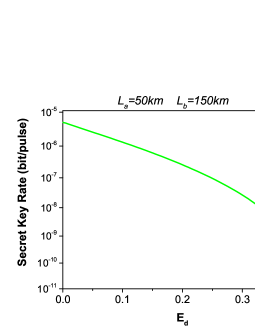
Figure 3: Secret key rate as a function of the $E_{d}$ when $L_{a}$=50km, $L_{b}$=150km.

Moreover, as we can see from Fig.3, in an asymmetric case, the SNS TF-QKD can tolerate very high misalignment errors, e.g., it can still generate secret keys even when $E_{d}$ exceeds 0.35. In original TF-QKD, the single-photon interference is a challenging technology and may cause large misalignment errors. While in the SNS TF-QKD, it only needs sending or-not sending pulses instead of interference in Z-window, and can thus tolerate much larger misalignment errors. In the present asymmetric case, the advantages hold on and make it very promising candidate in practical applications.

IV Summaries and outlooks

In conclusion, we have extended the SNS TF-QKD to the asymmetric case and given a general model. The lower bound of the yield and the upper bound of the QBER for single-photon contributions have been rederived. Then the asymmetry of channels could be compensated by optimizing the adjustable system parameters. Through implementing full parameter optimization on the numerical simulations, we demonstrate that our new method can dramatically improve the key generation rate and the transmission distance compared with the original symmetric method. In addition, some state-of-the-art optimization techniques, such as collective constraints and joint estimations can be applied to further improve the performance TFYu ; yu3 . Therefore, our work represent a further step towards practical application of the QKD.

We gratefully acknowledge the financial support from the National Key R$\&$D Program of China (Grant Nos. 2018YFA0306400, 2017YFA0304100), the National Natural Science Foundation of China (Grants Nos. 61475197, 61590932, 11774180, 61705110, 11847215), the China Postdoctoral Science Foundation (Grant No. 2018M642281), the Natural Science Foundation of Jiangsu Province (Grant No. BK20170902), the Jiangsu Planned Projects for Postdoctoral Research Funds(Grant No. 2018K185C), and the Postgraduate Research and Practice Innovation Program of Jiangsu Province (Grant No. KYCX17$\_$0791).

Appendix

Below, we will give a detailed derivation of Eq. (6). First, to get the monotonicity of $Y_{n}^{k}$, we make a formula deformation:

$$Y_{n}^{k}{\rm{=}}1-{(1-{P_{d}})^{2}}{[\frac{{k(1-{\eta_{a}})+(1-{\eta_{b}})}}{{k+1}}]^{n}}$$

$$=1-{(1-{P_{d}})^{2}}{[(1-{\eta_{a}})+\frac{{{\eta_{a}}-{\eta_{b}}}}{{k+1}}]^{n}}.$$ (13)

Obviously, when ${\eta_{a}}>{\eta_{b}}$, $Y_{n}^{k}$ is an increasing function of $k$.

The average gains of the two decoy-states is given by:

$${Q_{{\mu_{1}}}}={Y_{0}}{P_{0}}({\mu_{1}})+Y_{1}^{{k_{1}}}{P_{1}}({\mu_{1}})+Y_{2}^{{k_{1}}}{P_{2}}({\mu_{1}})+\sum\limits_{n=3}^{\infty}{Y_{n}^{{k_{1}}}{P_{n}}({\mu_{1}})},$$ (14)

$${Q_{{\mu_{2}}}}={Y_{0}}{P_{0}}({\mu_{2}})+Y_{1}^{{k_{2}}}{P_{1}}({\mu_{2}})+Y_{2}^{{k_{2}}}{P_{2}}({\mu_{2}})+\sum\limits_{n=3}^{\infty}{Y_{n}^{{k_{2}}}{P_{n}}({\mu_{2}})}.$$ (15)

When ${k_{1}}\leq{k_{2}}$, $Y_{n}^{k_{1}}\leq Y_{n}^{k_{2}}$ holds on. Eq.(15) can be expressed as:

$${Q_{{\mu_{2}}}}={Y_{0}}{P_{0}}({\mu_{2}})+Y_{1}^{{k_{1}}}{P_{1}}({\mu_{2}})+Y_{2}^{{k_{1}}}{P_{2}}({\mu_{2}})+\sum\limits_{n=3}^{\infty}{Y_{n}^{{k_{1}}}{P_{n}}({\mu_{2}})}+{\Delta_{1}},$$ (16)

where ${\Delta_{1}}=(Y_{1}^{{k_{2}}}-Y_{1}^{{k_{1}}}){P_{1}}({\mu_{2}})+(Y_{2}^{{k_{2}}}-Y_{2}^{{k_{1}}}){P_{2}}({\mu_{2}})+\sum\limits_{n=3}^{\infty}{(Y_{n}^{{k_{2}}}-Y_{n}^{{k_{1}}}){P_{n}}({\mu_{2}})}\geq 0$.

By using the similar method as in Ref. yu2 :

$${P_{2}}({\mu_{2}}){Q_{{\mu_{1}}}}={P_{2}}({\mu_{2}}){Y_{0}}{P_{0}}({\mu_{1}})+{P_{2}}({\mu_{2}})Y_{1}^{{k_{1}}}{P_{1}}({\mu_{1}})+{P_{2}}({\mu_{2}})Y_{2}^{{k_{1}}}{P_{2}}({\mu_{1}})+{P_{2}}({\mu_{2}})\sum\limits_{n=3}^{\infty}{Y_{n}^{{k_{1}}}{P_{n}}({\mu_{1}})},$$ (17)

$${P_{2}}({\mu_{1}}){Q_{{\mu_{2}}}}={P_{2}}({\mu_{1}}){Y_{0}}{P_{0}}({\mu_{2}})+{P_{2}}({\mu_{1}})Y_{1}^{{k_{1}}}{P_{1}}({\mu_{2}})+{P_{2}}({\mu_{1}})Y_{2}^{{k_{1}}}{P_{2}}({\mu_{2}})+{P_{2}}({\mu_{1}})\sum\limits_{n=3}^{\infty}{Y_{n}^{k1}{P_{n}}({\mu_{2}})}+{P_{2}}({\mu_{1}}){\Delta_{1}}.$$ (18)

Combining Eq.(17) and Eq.(18), we can get:

$${P_{2}}({\mu_{1}}){Q_{{\mu_{2}}}}-{P_{2}}({\mu_{2}}){Q_{{\mu_{1}}}}$$

$$= [{P_{2}}({\mu_{1}}){P_{0}}({\mu_{2}})-{P_{2}}({\mu_{2}}){P_{0}}({\mu_{1}})]{Y_{0}}+[{P_{2}}({\mu_{1}}){P_{1}}({\mu_{2}})-{P_{2}}({\mu_{2}}){P_{1}}({\mu_{1}})]Y_{1}^{{k_{1}}}$$

$$+{P_{2}}({\mu_{1}})\sum\limits_{n=3}^{\infty}{Y_{n}^{{k_{1}}}{P_{n}}({\mu_{2}})}-{P_{2}}({\mu_{2}})\sum\limits_{n=3}^{\infty}{Y_{n}^{{k_{1}}}{P_{n}}({\mu_{1}})}+{P_{2}}({\mu_{1}}){\Delta_{1}}.$$ (19)

Denote ${P_{2}}({\mu_{1}})\sum\limits_{n=3}^{\infty}{Y_{n}^{{k_{1}}}{P_{n}}({\mu_{2}})}-{P_{2}}({\mu_{2}})\sum\limits_{n=3}^{\infty}{Y_{n}^{{k_{1}}}{P_{n}}({\mu_{1}})}={\Delta_{2}}$. Due to the weak coherent source satisfying the following condition yu2 :

$$\frac{{{P_{n}}({\mu_{2}})}}{{{P_{n}}({\mu_{1}})}}\geq\frac{{{P_{2}}({\mu_{2}})}}{{{P_{2}}({\mu_{1}})}}\geq\frac{{{P_{1}}({\mu_{2}})}}{{{P_{1}}({\mu_{1}})}},$$ (20)

we can conclude that ${\Delta_{2}}>0$.

Finally, when ${k_{1}}\leq{k_{2}}$, the lower bound of the single-photon yield:

$$Y_{1}^{{k_{1}}}\geq Y_{1}^{L}=\frac{{{P_{2}}({\mu_{2}}){Q_{{\mu_{1}}}}-{P_{2}}({\mu_{1}}){Q_{{\mu_{2}}}}+[{P_{2}}({\mu_{1}}){P_{0}}({\mu_{2}})-{P_{2}}({\mu_{2}}){P_{0}}({\mu_{1}})]{Y_{0}}}}{{{P_{2}}({\mu_{2}}){P_{1}}({\mu_{1}})-{P_{2}}({\mu_{1}}){P_{1}}({\mu_{2}})}}.$$ (21)

References

- (1) H. K. Lo and H. F. Chau, Science 283, 2050 (1999).
- (2) P. W. Shor and J. Preskill, Phys. Rev. Lett. 85, 441 (2000).
- (3) D. Mayers, J. ACM 48, 351 (2001).
- (4) C. H. Bennett and G. Brassard, In Proceedings of the IEEE International Conference on Computers, Systems and Signal Processing (IEEE, New York, 1984), pp. 175-179.
- (5) W. Y. Hwang, Phys. Rev. Lett. 91, 057901 (2003).
- (6) X. B. Wang, Phys. Rev. Lett. 94, 230503 (2005).
- (7) H. K. Lo, X. F. Ma and K. Chen, Phys. Rev. Lett. 94, 230504 (2005).
- (8) S. L. Braunstein and S. Pirandola, Phys. Rev. Lett. 108, 130502 (2012).
- (9) H. K. Lo, M. Curty and B. Qi, Phys. Rev. Lett. 108, 130503 (2012).
- (10) S. Pirandola, R. Laurenza, C. Ottaviani, and L. Banchi, Nat. Commun. 8, 15043 (2017).
- (11) L. M. Duan, M. Lukin, J. I. Cirac, P. Zoller, Nature 414, 413 (2001).
- (12) N. Sangouard, C. Simon, H. de Riedmatten, N. Gisin, Rev. Mod. Phys. 83, 33 (2011).
- (13) M. Lucamarini, Z. L. Yuan, J. F. Dynes, and A. J. Shields, Nature (London) 557, 400 (2018).
- (14) X. F. Ma, P. Zeng, and H. Y. Zhou, Phys. Rev. X 8, 031043 (2018).
- (15) X. B. Wang, Z. W. Yu, and X.-L. Hu, Phys. Rev. A 98, 062323 (2018).
- (16) J. Lin and N. Lütkenhaus, Phys. Rev. A 98, 042332 (2018).
- (17) M. Curty, K. Azuma, and H. K. Lo, arXiv:1807.07667.
- (18) K. Tamaki, H. K. Lo, W. Y. Wang, and M. Lucamarini, arXiv:1805.05511.
- (19) Z. W. Yu, X. L. Hu, C. Jiang, H. Xu, and X. B. Wang, arXiv:1807.09891.
- (20) C. H. Cui, Z. Q. Yin, R. Wang, F. Y. Lu, W. Chen, S. Wang, G. C. Guo, and Z. F. Han, arXiv:1807.02334
- (21) H. L. Yin, Y. Fu, arXiv:1805.12004.
- (22) F. Xu, M. Curty, B. Qi, and H. K. Lo, New J. Phys. 15, 113007 (2013).
- (23) X. L. Hu, Y. Cao, Z. W. Yu, and X. B. Wang, Sci. Rep. 8, 17634(2018).
- (24) W. Wang, F. Xu, and H. K. Lo, arXiv:1807.03466.
- (25) Z. W. Yu, Y. H. Zhou and X. B. Wang, Phys. Rev. A 91, 032318 (2015).
- (26) Y. H. Zhou, Z. W. Yu and X. B. Wang, Phys. Rev. A, 93, 042324 (2016).