When Causal Intervention Meets Adversarial Examples and Image Masking for Deep Neural Networks

Abstract

Discovering and exploiting the causality in deep neural networks (DNNs) are crucial challenges for understanding and reasoning causal effects (CE) on an explainable visual model. ”Intervention” has been widely used for recognizing a causal relation ontologically. In this paper, we propose a causal inference framework for visual reasoning via do-calculus. To study the intervention effects on pixel-level features for causal reasoning, we introduce pixel-wise masking and adversarial perturbation. In our framework, CE is calculated using features in a latent space and perturbed prediction from a DNN-based model. We further provide the first look into the characteristics of discovered CE of adversarially perturbed images generated by gradient-based methods . Experimental results show that CE is a competitive and robust index for understanding DNNs when compared with conventional methods such as class-activation mappings (CAMs) on the Chest X-Ray-14 dataset for human-interpretable feature(s) (e.g., symptom) reasoning. Moreover, CE holds promises for detecting adversarial examples as it possesses distinct characteristics in the presence of adversarial perturbations.

Index Terms—  Causal Reasoning, Adversarial Example, Adversarial Robustness, Interpretable Deep Learning

1 Introduction

In recent years, deep neural networks (DNNs) based models have demonstrated a significant improvement in state-of-the-art results for several vision tasks [1, 2]. Despite their effectiveness, DNNs are notoriously cryptic for their complexity, opacity, and lacking apparent relationship between neural architecture and the function being evaluated by the network. These challenges are amplified especially when DNN models show superior performance over conventional methods (e.g., decision-trees) on human-interpretable feature learning tasks, such as clinical (i.e., cancer recognition [3]), emotional (i.e., violence detection [4]), and social (i.e., behavior reasoning [5]) patterns recognition, where even experts did not fully reach a proper consensus. Therefore, interpretability [6] and explainable reasoning features of DNNs remain challenging. From regulatory aspects (e.g., GDPR [7]), human-interpretable feature selection is crucial for administrative decision-making, as current DNNs highly depend on supervised labels generated by human knowledge but barely explain the learned relationship between its labeled input-feature(s) and predicted output(s). The importance of reasoning is also motivated by demystifying the vulnerable properties of DNNs against adversarial examples [8, 9, 10].

This paper studies the problems of causal interpretability on DNNs for vision tasks. We propose a new visual reasoning method inspired by causal inference embedded DNNs and verify its sensitivity on input masking and adversarial perturbations. We summarize some input intervention-based explanation methods for DNNs as follows.

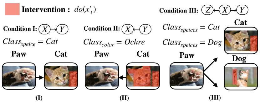
Fig. 1: Visual intervention in three classical causal conditions [11]: (I) $X\rightarrow{}Y$ for single class counterfactual reasoning; (II) $X\leftarrow{}Y$ for multi-classes counterfactual reasoning, and (III) $Z\leftarrow{}X\rightarrow{}Y$ for conditional multitasking counterfactual reasoning of a visual perceptual-model.

Saliency map based method. Many works employ saliency map for visual explanations. Class activation mappings [12] (CAMs) have provided visual explanations via tracing gradient-based localization. Gradient information from a penultimate convolutional layer was used in GradCAM [13] to identify discriminating patterns in input images. However, CAM-based methods have some limitations on causal reaonsing. They could only conclude that a DNN model would feature with certain localized patterns. Denoting a trained DNNs model as $Y$ and input data as $X$, CAM-based mothods can be viewed as a reverse causation (e.g., $X_{input}\xrightarrow[\overleftarrow{CAM}]{\textbf{DNN Model }}Y_{output}$). Saliency maps [12, 13] only establish a correlation for interpretability while it is possible to trace a particular image region that is responsible for it to be correctly classified; it cannot elucidate what would happen if a certain portion of the image was masked out. See [11] for a What If question, when a classifier is used in the wild. In addition to this causal reasoning weakness, recent study also shows CAMs barely preserve robustness from a gradient adversarial attacks as a secure reasoning index [14].
Adversarial robustness. Although there has recently been a great deal of research in adversarial defenses, many of these methods are later shown to be broken [15]. The most common, “brute force” solution is adversarial training, where we simply include a mixture of normal and adversarially-generated examples in the training set [16]. One obvious limitation of previous work is the robustness generalizability for adversarial examples beyond the pre-defined norm or distributional constraints.
Causal reasoning. Building causal interpretations toward evaluating a robust and interpretable DNNs are still largely unexplored. Causality as a means of explanation has deep roots for factor selection and has received many attentions. The rest of this paper is presented as follows. First, we describe a general framework to build a causal inference to reason over a targeted DNN model via intervention. Second, we discover adversarial robustness between causal factor. Lastly, we propose an adversary-sensitive feature-map to visualize the causal effects of interpreterable features (e.g., symptoms) toward large-scale medical datasets by using DenseNet [2]. Our contributions include:

• The design of a causal inference framework for calculating CE on single task, multi-labels, and multitasking vision tasks. An autoencoder network has been introduced for intervening interpretable feature(s).

• The investigation of CE toward highlighting counterfactual intervention by pixel-wise masking and adversarial settings.

• A case study for learning the causal effects from a large-scale medical dataset (Chest X-Ray-14) for reasoning related chest symptoms by Causal Effect Map (CEM).

2 Related Works

Causal models have been advocated as a proper method [17] for parameter reasoning in a complex system. Modeling bias and fairness as a counterfactual [17] is a new way to quantify the bias of models. Ideas from causal inference have also been used in providing comprehensive explanations of deep learning models. In [18], a method is developed to build a causal model over human-centric image-based abstractions of the model, which helps provide the ability to allow users to propose comprehensive queries. With an interpretable concept, the method could learn a causal model relating to network activations and features for classifications. Moreover, as DNNs can be viewed as a graphical model for inference, recent work in [19] proposed using Structural Causal Models (SCM) to reason over a deep-learning model. The technique includes building the direct acyclic graph (DAG) structure from the DNN, applying a suitable transformation and estimating the causal effect using causal inference.

3 Visual Causal Intervention

3.1 Causal Theory

We adopt the widely-accepted Causal Effect (CE) from Pearl’s do-calculus for $do(X_{i}=x_{i})\equiv x_{i}=f_{i}(pa_{i},u_{i})$, where $pa_{i}$ are the parents of variable $X_{i}$ in a graph, $G$. Selecting two disjoint sets of random variables, $X$ and $Y$, the causal effect of $X$ on $Y$ is denoted as $P(y|do(x))$, which is a function from $X$ to the space of probability distributions on $Y$. As an illustration, here we introduce a graph $G$ including random variables $\mathbf{X,Y,Z}$ in Figure 1 for constructing elemental causal networks for this study.
Computing the Effect of Intervention An atomic intervention do($X_{i}=x^{\prime}_{i}$) has been used in the previous study [18] as a $truncated~{}factorization$ for feature selection in a latent space of a targeted DNN system for causal reasoning. Given a joint distribution P($\mathbf{O},\mathbf{P},\mathbf{X}$), over a set of DNN with outputs $\mathbf{O}$, inputs $\mathbf{P}$, and intermediate variables $\mathbf{X}$, from the definition in [20], measuring CE of an intervention on $x^{\prime}_{i}$ on $X_{j}=x_{j}$ with all of the evidence $Z$ could be computed as:

$$Effect(x_{i}\rightarrow{}x_{j},Z)=P(x_{j}|do(x_{i}^{\prime}),Z_{X_{i}})-P(x_{j}|Z_{X_{i}})$$ (1)

The excepted casual effect from Eqn. 6 in [18] has been defined as:

$$E_{X_{i}}[Effect(x_{i}\rightarrow{}x_{j},Z)]=\sum_{x_{i}\in X_{i}}P(X_{i}=x_{i}|Z)\times(1)$$ (2)

Then, we adapt the method in (2) on DNN model with (I) single task, (II) multiple tasks, and (III) multiple labels from Figure.1 for computing expected-CE analysis, where $Z_{X_{i}}$ is a counterfactual setting.
Interventions as Variables Different from previous approaches to directly measuring the intervened result for calculating CE, alternatively, an intervention $do(X_{i}=x^{\prime}_{i})$ could be encoded by adding to $G$ a link $F_{i}\rightarrow{X_{i}}$, where $F_{i}$ is a new variable taking values in $\left\{do(x^{\prime}_{i}),idle\right\}$. Here, the notion of $``idle"$ means “no intervention” following Pearl’s Eqn. 3.8 [11]. In this paper, we adapt this concept by introducing masking and adversarial intervention as $F_{i}$ variables for discovering CE within the DNN in a zero-out evident state, $Z_{0}$. This conditional probability could be calculated by:

$$P(x_{i}|pa^{\prime}_{i})=\left\{\begin{matrix}P(x_{i}|pa_{i})&if~{}F_{1}=idle,\\ 0&if~{}F_{i}=do(x^{\prime}_{i})~{}and~{}x_{i}\neq x^{\prime}_{i},\\ 1&if~{}F_{i}=do(x^{\prime}_{i})~{}and~{}x_{i}=x^{\prime}_{i}.\end{matrix}\right.$$ (3)

The advantages of this augmented causal graph in (3) are its capability for showing the ramification of spontaneous change in $f_{i}$ from $F_{i}$ instead of merely replacing $f_{i}$ by a constant.

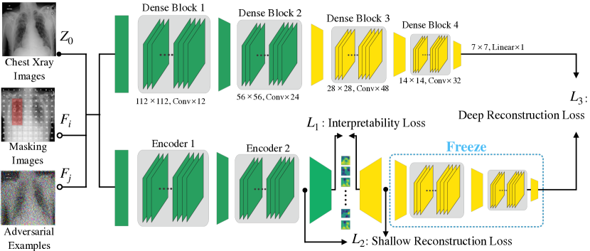
Fig. 2: Framework and deep network topology. We use pixel-wise masking as $F_{i}$ and adversarial examples as $F_{j}$ intervention variables in the $Z_{0}$ (zero-out) counterfactual setting.

3.2 Concept extraction by Autoencoder

Autoencoder networks Our autoencoder consists of five convolutional layers. The encoder and decoder each have two symmetrical layers, and they aim to capture the textural features corresponding to human visual perception. However, our decoder reconstructs slightly altered network activations while ensuring significant downstream network activations are unaffected. We mainly designed a low-dimensional layer in the middle to integrate scattered features into concepts. This is inspired by how our brain pays attention, processes information and interpretsthe perceived inputs.
Build up a Causal Baseline To attain better causality measurement, we trained our model with a designed loss function composed of three parts from the existing studies [18] as casual baseline: interpretability loss, shallow reconstruction loss, and deep reconstruction loss. Shallow reconstruction loss is simply the $L_{1}$ norm of the difference between the input and output of autoencoder to represent the activations of the network. Also, we applied the deep reconstruction loss in the form of the KL-divergence between the output probability distribution of original and autoencoder-inserted network. Our total loss function for the causality model is (from Harradon et al. 2018 Eqn. 7 in [18]):
$L(\theta;x_{i})=\lambda_{shallow}\times L_{shallow}(\theta;x_{i})+\lambda_{deep}\times L_{deep}(\theta;x_{i})\\ \indent\indent\indent+\lambda_{interpretability}\times L_{interpretability}(\theta;x_{i})$ (3)
Our method is based on the proposed loss in the previous work [18] to reproduce the measurement of causality.

3.3 Intervention Methods

In the zero-out ($Z_{0}$) setting, we discuss two types of perturbation as independent intervention variables for computing expected-CE: (1) pixel-wise masking (PWM) and (2) adversarial noise. The purpose of pixel-wise perturbation, $F_{i}$, is to recognize the causal relationship between a local pixel and the final output result of a DNN. We apply the following adversarial noises on images as another intervention $F_{j}$.
Fast Gradient Sign Method (FGSM) Fast Gradient Sign Method (FGSM) [21] is a gradient-based adversarial noise to generate adversarial examples by one step gradient update along the direction of the sign of gradient at each pixel.
Jacobian-Based Saliency Map (JBSM) Attack Papernot et al. [22] designed an efficient saliency adversarial map, called Jacobian-based Saliency Map Attack by saturating a few pixels in a given image to their maximum or minimum values.
BIM and PGD Attacks Kurakin et al. [16] applied extended Fast Gradient Sign method by running a finer optimization (smaller change) for multiple iterations Basic Iterative Method (BIM) attack. Projected gradient descent (PGD) attack has been introduced by subjecting to a constraint [16].

4 Experiments

We use three benchmark image datasets which have been proved robust to reassure that the causal effect would not be compromised by the defect of data. The datasets are fashion-MNIST, ImageNet and NIH-ChestX-Ray-14. We investigate $X\rightarrow{}Y$ for single feature causal intervention. For adversarial setting in our experiments, we use maximum $L_{\infty}$ perturabtion strength $\epsilon$ = $0.3$ and iterative steps = 10.
Numerical Validation on Bird Dataset In previous work, the VGG19 [23] model applied to bird200 [24] had significant causal effect with intervention at layer 18 feature 2. In our work, we also use VGG19 to reproduce the procedure and test the causality by intervening the same position. The expect causal effect is $7.6341\times 10^{-3}$, which suffices to validate our method and proved the potential of better interpretability.

4.1 Quantitative Study on NIH-ChestX-Ray-14

NIH-ChestX-Ray-14 [25] is the largest available chest Xray dataset. Despite of anatomical obstacles, CheXNet model could attain competitive classification performance with radiologists [26]. Different from various classes in ImageNet, the interpretable patterns in ChestX-ray14 are clinical symptoms, which could only be recognized by radiologists and hardly identified by CAM against adversarial setting in Figure 3.
CheXNet We implemented CheXNet [26] as a 121-layer convolutional neural network trained on ChestX-ray14 dataset contains frontal-view chest X-ray images and labeled with up to 14 different thoracic diseases. We modified the DenseNet121 model by replacing the final fully connected layer and apply a sigmoid layer. We use Adam with 0.001 learning rate, $\beta 1$ as 0.9, $\beta 2$ as 0.999. We choose binary cross entropy, and the classifier ended up achieved 85.08% accuracy. Besides, we investigate $Y\rightarrow{}X$ by masking the known symptoms and generate negative Expected-CE as ${-1.624}\times 10^{-4}$, which provides inference. For $Z\leftarrow{}X\rightarrow{}Y$, we zero-out the nodes which activate additional feature identified as a pulmonary disease as an additional label suggested by a pulmonologist. However, CE of this multitasking reasoning is not obvious. Intervention by pixel-wise Masking For PWM, we intervene with the visual traits of inputs. We mask 10 % area of the images randomly to explore the impact of masking on the causal effect. We could assure the intervention without bias with a chance to observe the region of interest of the causal model. The results in Table 1, 3, and 4 show the value of Expected-CE deceases by PWM, which indicate a declined causal importance inferences by pixel-wise perturbation.
Intervention by Adversarial Attacks From Table 2., we observe a numerical difference of Expected-CE by four gradient-based adversarial attacks, where FGSM has a larger negative causal effect with -5.6129 $\times 10^{-6}$. We then adapt FGSM to evaluate generic datasets in Section 4.2.

The presence of malicious adversarial-noise via CAMs such as (I) in Fig. 3 is often hardly to detect if the dataset has similar visual patterns (e.g., clinical patterns). We propose an adversary-sensitive causal effect map (CEM) by activated weights of CE in Eqn. 1 on each pixel toward classifying a specific class.

Table 1: Expected-CE on CheXNet

Level(L), Node(N)	$Z_{0}$	$F_{i}$ = PWM
3,4	4.5076$\times 10^{-3}$	7.2356$\times 10^{-7}$
6,5	2.843$\times 10^{-3}$	1.2154$\times 10^{-5}$
6,10	3.1939$\times 10^{-3}$	9.0066$\times 10^{-6}$
8,5	3.1939$\times 10^{-3}$	1.1536$\times 10^{-5}$
10,7	1.3775$\times 10^{-2}$	-1.1506$\times 10^{-5}$

Table 2: CheXNet ($F_{j}$ on L = 10, N = 7)

$F_{j}$ = Types of Adversarial Attack	Expected-CE
FSGM	-5.6129$\times 10^{-6}$
BIM	4.3435$\times 10^{-5}$
JBSM	7.7548$\times 10^{-5}$
PGD	-3.9605$\times 10^{-6}$

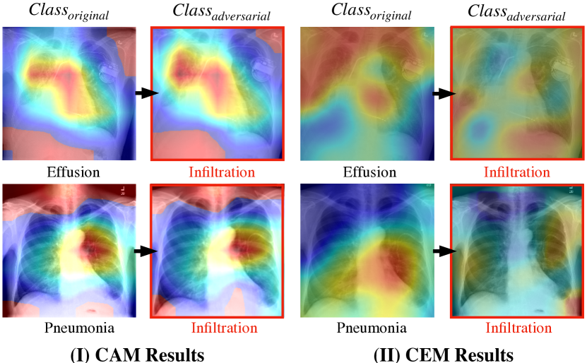
Fig. 3: Sensitivity for adversarial setting between (I) Class Activation Map (CAM) [12] and (II) Causal Effect Map (CEM) on ChestX-ray 14 for clinical symptoms labels [26].

4.2 Other Image Classification Datasets

Fashion-MNIST The fashion-MNIST dataset comprises of 28$\times$28 grayscale images of 70,000 fashion products from 10 categories, with 7,000 images per category. [27]. We use shallow model consists of 2 convolutional layers. The weights are trained using Adam with initial learning rate 0.001. We train the model using minibatches of size 100. The classifier with lowest validation loss has 89.6% accuracy.

Table 3: Expected-CE on Fashion-MNIST

L, N	$Z_{0}$	$F_{i}$ = PWM	$F_{j}$ = FGSM
2,3	4.9543$\times 10^{-4}$	-1.8947$\times 10^{-5}$	-8.0042$\times 10^{-6}$
2,7	2.4600$\times 10^{-4}$	-4.1068$\times 10^{-5}$	-2.5742$\times 10^{-5}$

ImageNet The ImageNet [28] 2012 classification dataset consists 1.2 million images for training, and 50,000 for validation, from 1, 000 classes. As a benchmark dataset, we use it to demonstrate visual causality. We use VGG16 model which has 16 convolutional layers and is pretrained by ImageNet with 86% top-1 accuracy.

Table 4: Expected-CE on ImageNet

L, N	$Z_{0}$	$F_{i}$ = PWM	$F_{j}$ = FGSM
3,2	4.2027$\times 10^{-4}$	6.0993$\times 10^{-5}$	-5.1834$\times 10^{-5}$
9,10	8.9322$\times 10^{-3}$	7.2438$\times 10^{-5}$	- 2.8862$\times 10^{-4}$
13,6	6.7643$\times 10^{-4}$	2.3943$\times 10^{-6}$	-6.8749$\times 10^{-5}$

4.3 Evaluation of Causal Effect

To validate the reliability of our approach, we also implemented our causal inference framework on Fashion-MNIST and ImageNet. We applied random pixel-wise feature masking and adversarial noise separately to the input images with $Z_{0}$ coded feature map. Table 3 and 4 show that comparing to $Z_{0}$, Expected-CE of these two datasets decreased drastically once we applied random masking and adversarial noise, which are similar to the results of CheXNet. The results suggest that our causality framework is generic and can be applied to different datasets (please refer our reproducible code.)

5 Conclusion

With our proposed framework, experimental results on Fashion-MNIST, ImageNet, and ChestX-ray14 datasets show that CE is a competitive and robust index for understanding DNNs for generic and human-interpretable feature(s) reasoning. CE also shows high sensitivity in the presence of adversarial perturbations and could be used to identify adversarial examples.

References

- [1] Serena Yeung, Olga Russakovsky, Greg Mori, and Li Fei-Fei, “End-to-end learning of action detection from frame glimpses in videos,” in Proceedings of the IEEE Conference on Computer Vision and Pattern Recognition, 2016, pp. 2678–2687.
- [2] Gao Huang, Zhuang Liu, Laurens Van Der Maaten, and Kilian Q Weinberger, “Densely connected convolutional networks,” in Proceedings of the IEEE conference on computer vision and pattern recognition, 2017, pp. 4700–4708.
- [3] Andre Esteva, Brett Kuprel, Roberto A Novoa, Justin Ko, Susan M Swetter, Helen M Blau, and Sebastian Thrun, “Dermatologist-level classification of skin cancer with deep neural networks,” Nature, vol. 542, no. 7639, pp. 115, 2017.
- [4] Waqas Sultani, Chen Chen, and Mubarak Shah, “Real-world anomaly detection in surveillance videos,” Center for Research in Computer Vision (CRCV), University of Central Florida (UCF), 2018.
- [5] Yingxu Wang, “Deep reasoning and thinking beyond deep learning by cognitive robots and brain-inspired systems,” in Cognitive Informatics & Cognitive Computing (ICCI* CC), 2016 IEEE 15th International Conference on. IEEE, 2016, pp. 3–3.
- [6] Quanshi Zhang, Ying Nian Wu, and Song-Chun Zhu, “Interpretable convolutional neural networks,” in Proceedings of the IEEE Conference on Computer Vision and Pattern Recognition, 2018, pp. 8827–8836.
- [7] Jan Philipp Albrecht, “How the gdpr will change the world,” Eur. Data Prot. L. Rev., vol. 2, pp. 287, 2016.
- [8] Ian J Goodfellow, Jonathon Shlens, and Christian Szegedy, “Explaining and harnessing adversarial examples,” ICLR, 2015.
- [9] Battista Biggio and Fabio Roli, “Wild patterns: Ten years after the rise of adversarial machine learning,” Pattern Recognition, vol. 84, pp. 317–331, 2018.
- [10] Dong Su, Huan Zhang, Hongge Chen, Jinfeng Yi, Pin-Yu Chen, and Yupeng Gao, “Is robustness the cost of accuracy?–a comprehensive study on the robustness of 18 deep image classification models,” in ECCV, 2018, pp. 631–648.
- [11] Judea Pearl, Causality, Cambridge university press, 2009.
- [12] Bolei Zhou, Aditya Khosla, Agata Lapedriza, Aude Oliva, and Antonio Torralba, “Learning deep features for discriminative localization,” in Proceedings of the IEEE Conference on Computer Vision and Pattern Recognition, 2016, pp. 2921–2929.
- [13] Ramprasaath R Selvaraju, Michael Cogswell, Abhishek Das, Ramakrishna Vedantam, Devi Parikh, and Dhruv Batra, “Grad-cam: Visual explanations from deep networks via gradient-based localization,” in 2017 IEEE International Conference on Computer Vision (ICCV). IEEE, 2017, pp. 618–626.
- [14] Aaditya Prakash, Nick Moran, Solomon Garber, Antonella DiLillo, and James Storer, “Deflecting adversarial attacks with pixel deflection,” in Proceedings of the IEEE Conference on Computer Vision and Pattern Recognition, 2018, pp. 8571–8580.
- [15] Anish Athalye, Nicholas Carlini, and David Wagner, “Obfuscated gradients give a false sense of security: Circumventing defenses to adversarial examples,” ICML, 2018.
- [16] Alexey Kurakin, Ian Goodfellow, and Samy Bengio, “Adversarial examples in the physical world,” arXiv preprint arXiv:1607.02533, 2016.
- [17] Matt J Kusner, Joshua Loftus, Chris Russell, and Ricardo Silva, “Counterfactual fairness,” in Advances in Neural Information Processing Systems, 2017, pp. 4066–4076.
- [18] Michael Harradon, Jeff Druce, and Brian Ruttenberg, “Causal learning and explanation of deep neural networks via autoencoded activations,” arXiv preprint arXiv:1802.00541, 2018.
- [19] Tanmayee Narendra, Anush Sankaran, Deepak Vijaykeerthy, and Senthil Mani, “Explaining deep learning models using causal inference,” arXiv preprint arXiv:1811.04376, 2018.
- [20] Paul R Rosenbaum and Donald B Rubin, “Assessing sensitivity to an unobserved binary covariate in an observational study with binary outcome,” Journal of the Royal Statistical Society: Series B (Methodological), vol. 45, no. 2, pp. 212–218, 1983.
- [21] Michael Goodfellow and Amanda L Jones, “Laceyella,” Bergey’s Manual of Systematics of Archaea and Bacteria, pp. 1–4, 2015.
- [22] Nicolas Papernot, Patrick McDaniel, Xi Wu, Somesh Jha, and Ananthram Swami, “Distillation as a defense to adversarial perturbations against deep neural networks,” in 2016 IEEE Symposium on Security and Privacy (SP). IEEE, 2016, pp. 582–597.
- [23] Karen Simonyan and Andrew Zisserman, “Very deep convolutional networks for large-scale image recognition,” arXiv preprint arXiv:1409.1556, 2014.
- [24] Steve Branson, Catherine Wah, Florian Schroff, Boris Babenko, Peter Welinder, Pietro Perona, and Serge Belongie, “Visual recognition with humans in the loop,” in European Conference on Computer Vision. Springer, 2010, pp. 438–451.
- [25] Xiaosong Wang, Yifan Peng, Le Lu, Zhiyong Lu, Mohammadhadi Bagheri, and Ronald Summers, “Chestx-ray8: Hospital-scale chest x-ray database and benchmarks on weakly-supervised classification and localization of common thorax diseases,” in 2017 IEEE Conference on Computer Vision and Pattern Recognition(CVPR), 2017, pp. 3462–3471.
- [26] Pranav Rajpurkar, Jeremy Irvin, Kaylie Zhu, Brandon Yang, Hershel Mehta, Tony Duan, Daisy Ding, Aarti Bagul, Curtis Langlotz, Katie Shpanskaya, et al., “Chexnet: Radiologist-level pneumonia detection on chest x-rays with deep learning,” arXiv preprint arXiv:1711.05225, 2017.
- [27] Han Xiao, Kashif Rasul, and Roland Vollgraf, “Fashion-MNIST: a Novel Image Dataset for Benchmarking Machine Learning Algorithms,” arXiv e-prints, p. arXiv:1708.07747, Aug. 2017.
- [28] Jia Deng, Wei Dong, Richard Socher, Li-Jia Li, Kai Li, and Li Fei-Fei, “Imagenet: A large-scale hierarchical image database,” in Computer Vision and Pattern Recognition, 2009. CVPR 2009. IEEE Conference on. Ieee, 2009, pp. 248–255.