Probably the Best Itemsets

Abstract

One of the main current challenges in itemset mining is to discover a small set of high-quality itemsets. In this paper we propose a new and general approach for measuring the quality of itemsets. The method is solidly founded in Bayesian statistics and decreases monotonically, allowing for efficient discovery of all interesting itemsets. The measure is defined by connecting statistical models and collections of itemsets. This allows us to score individual itemsets with the probability of them occuring in random models built on the data.

As a concrete example of this framework we use exponential models. This class of models possesses many desirable properties. Most importantly, Occam’s razor in Bayesian model selection provides a defence for the pattern explosion. As general exponential models are infeasible in practice, we use decomposable models; a large sub-class for which the measure is solvable. For the actual computation of the score we sample models from the posterior distribution using an MCMC approach.

Experimentation on our method demonstrates the measure works in practice and results in interpretable and insightful itemsets for both synthetic and real-world data.

1 Introduction

Discovering frequent itemsets is one of the most active fields in data mining. As a measure of quality, frequency possesses a lot of positive properties: it is easy to interpret and as it decreases monotonically there exist efficient algorithms for discovering large collections of frequent itemsets [2]. However, frequency also has serious drawbacks. A frequent itemset may be uninteresting if its elevated frequency is caused by frequent singletons. On the other hand, some non-frequent itemsets could be interesting. Another drawback is the problem of pattern explosion when mining with a low threshold.

Many different quality measures have been suggested to overcome the mentioned problems (see Section 5 for a more detailed discussion). Usually these measures compare the observed frequency to some expected value derived, for example, from the independence model. Using such measures we may obtain better results. However, these approaches still suffer from pattern explosion. To point out the problem, assume that two items, say $a$ and $b$ are correlated, and hence are considered significant. Then any itemset containing $a$ and $b$ will be also considered significant.

Example 1

Assume a dataset with $K$ items $a_{1},\ldots,a_{K}$ such that $a_{1}$ and $a_{2}$ always yield identical value and the rest of the items are independently distributed. Assume that we apply some statistical method to evaluate the significance of itemsets by using the independence model as the ground truth. If an itemset $X$ contains $a_{1}a_{2}$, its frequency will be higher than then the estimate of the independence model. Hence, given enough data, the P-value of the statistical test will go to $0$, and we will conclude that the itemset $X$ is interesting. Consequently we will find $2^{K-2}$ interesting itemsets.

In this work we approach the problem of defining quality measure from a novel point of view. We construct a connection between itemsets and statistical models and use this connection to define a new quality measure for itemsets. To motivate this approach further, let us consider the following example.

Example 2

Consider a binary dataset with $5$ items, say $a_{1},\ldots,a_{5}$, generated from the independence model. We argue that if we know that the data comes from the independence model, then the only interesting itemsets are the singletons. The reasoning behind this claim is that the frequencies of singletons correspond exactly to the column margins, the parameters of the independence model. Once we know the singleton frequencies, there is nothing left in the data that would be statistically interesting.

Let us consider a more complicated example. Assume that data is generated from a Chow-Liu tree model [4], say

$$p(A)=p(a_{1})p(a_{2}\mid a_{1})p(a_{3}\mid a_{1})p(a_{4}\mid a_{2})p(a_{5}\mid a_{4}).$$

Again, if we know that data is generated from this model, then we argue that the interesting itemsets are $a_{1}$, $a_{2}$, $a_{3}$, $a_{4}$, $a_{5}$, $a_{1}a_{2}$, $a_{1}a_{3}$, $a_{2}a_{4}$, and $a_{4}a_{5}$. The reasoning here is the same as with the independence model. If we know the frequencies of these itemsets we can derive the parameters of the distribution. For example, $p(a_{2}=1\mid a_{1}=1)=\mathit{fr}\mathopen{}\left(a_{1}a_{2}\right)/\mathit{fr}\mathopen{}\left(a_{1}\right)$.

Let us now demonstrate that this approach will produce much smaller and more meaningful output than the method given in Example 1.

Example 3

Consider the data given in Example 1. To fully describe the data we only need to know the frequencies of the singletons and the fact that $a_{1}$ and $a_{2}$ are identical. This information can be expressed by outputting the frequencies of singleton itemsets and the frequency of itemset $a_{1}a_{2}$. This will give us $K+1$ interesting patterns in total.

Our approach is to extend the idea pitched in the preceding example to a general itemset mining framework. In the example we knew which model generated the data, in practice, we typically do not. To solve this we will use the Bayesian approach, and instead of considering just one specific model, we will consider a large collection of models, namely exponential models. A virtue of these models is that we can naturally connect each model to certain itemsets. A model $M$ has a posterior probability $P(M\mid D)$, that is, how probable is the model given the data. The score of a single itemset then is just the probability of it being a parameter of a random model given the data. This setup fits perfectly the given example. If we have strong evidence that data is coming from the independence model, say $M$, then the posterior probability $P(M\mid D)$ will be close to $1$, and the posterior probability of any other model will be close to $0$. Since the independence model is connected to the singletons, the score for singletons will be $1$ and the score for any other itemset will be close to $0$.

Interestingly, using statistical models for defining significant itemsets provides an approach to the problem of the pattern set explosion (see Section 3.2 for more technical details). Bayesian model selection has an in-built Occam’s razor, favoring simple models over complex ones. Our connection between models and itemsets is such that simple models will correspond to small collections of itemsets. In result, only a small collection of itemsets will be considered interesting, unless the data provides sufficient amount of evidence.

Our contribution in the paper is two-fold. First, we introduce a general framework of using statistical models for scoring itemsets in Section 2. Secondly, we provide an example of this framework in Section 3 by using exponential models and provide solid theoretical evidence that our choices are well-founded. We provide the sampling algorithm in Section 4. We discuss related work in Section 5 and present our experiments in Section 6. Finally, we conclude our work with Section 7. The proofs are given in Appendix. The implementation is provided for research purposes.

2 Significance of Itemsets by Statistical Models

As we discussed in the introduction, our goal is to define a quality measure for itemsets using statistical models. In this section we provide a general framework for such a score. We will define the actual models in the next section.

We begin with some preliminary definitions and notations. In our setup a binary dataset is a collection of $N$ transactions, binary vectors of length $K$. We assume that these vectors are independently generated from some unknown distribution. Such a dataset can be easily represented by a binary matrix of size $N\times K$. By an attribute $a_{i}$ we mean a Bernoulli random variable corresponding to the $i$th column of the data. We denote the set of attributes by $A=\left\{a_{1},\ldots,a_{K}\right\}$.

An itemset $X$ is simply a subset of $A$. Given an itemset $X=\left\{a_{i_{1}},\ldots,a_{i_{L}}\right\}$ and a transaction $t$ we denote by $t_{X}=\left(t_{i_{1}},\ldots,t_{i_{L}}\right)$ the projection of $t$ into $X$. We say that $t$ covers $X$ if all elements in $t_{X}$ are equal to 1.

We say that a collection of itemsets $\mathcal{F}$ is downward closed if for each member $X\in\mathcal{F}$ any sub-itemset is also included. This property plays a crucial point in mining frequent patterns since it allows effective candidate pruning in level-wise approach and branch pruning in a DFS approach.

Our next step is to define the correspondence between statistical models and families of itemsets. Assume that we have a set $\mathcal{M}$ of statistical models for the data. We will discuss in later sections what specific models we are interested in, but for the moment, we will keep our discussion on a high level. Each model $M\in\mathcal{M}$ has a posterior probability $P(M\mid D)$, that is, how probable the model $M$ is given data $D$. To link the models to families of itemsets we assume that we have a function $\mathit{fam}$ that identifies a model $M$ with a downward closed family of itemsets. As we will see later on, there is one particular natural choice for such a function.

Now that we have our models that are connected to certain families of itemsets, we are ready to define a score for individual itemsets. The score for an itemset $X$ is the posterior probability of $X$ being a member in a family or itemsets,

$$sc\mathopen{}\left(X\right)=\sum_{X\in\mathit{fam}\mathopen{}\left(M\right),\atop M\in\mathcal{M}}P(M\mid D).$$ (1)

The motivation for such score is as follows. If we are sure that some particular model $M$ is the correct model for $D$, then the posterior probability for that model will be close to $1$ and the posterior probabilities for other models will be close to $0$. Consequently, the score for an itemset $X$ will be close to $1$ if $X\in\mathit{fam}\mathopen{}\left(M\right)$, and $0$ otherwise.

Naturally, the pivotal choice of this score lies in the mapping $\mathit{fam}$. Such a mapping needs to be statistically well-founded, and especially the size of an itemset family should be reflected in the complexity of the corresponding model. We will see in the following section that a particular choice for the model family and mapping $\mathit{fam}$ has these properties, and leads to certain important qualities.

Proposition 4

The score decreases monotonically, that is, $X\subseteq Y$ implies $sc\mathopen{}\left(X\right)\geq sc\mathopen{}\left(Y\right)$.

Proof 2.5.

We are allowing $\mathit{fam}$ only to map on downward closed families. Hence the inequality

$$\sum_{X\in\mathit{fam}\mathopen{}\left(M\right),\atop M\in\mathcal{M}}P(M\mid D)\geq\sum_{Y\in\mathit{fam}\mathopen{}\left(M\right),\atop M\in\mathcal{M}}P(M\mid D)$$

holds, and consequently we have $sc\mathopen{}\left(X\right)\geq sc\mathopen{}\left(Y\right)$. This completes the proof.

3 Exponential Models

In this section we will make our framework more concrete by providing a specific set $\mathcal{M}$ of statistical models and the function $\mathit{fam}$ identifying the models with families of itemsets. We will first give the definition of the models and the mapping. After this, we point out the main properties of our model and justify our choices. However, as, it turns out that computing the score for these models is infeasible, so instead, we solve this problem by considering decomposable models.

3.1 Definition of the models

Models of exponential form have been studied exhaustively in statistics, and have been shown to have good theoretical and practical properties. In our case, using exponential models provide a natural way of describing the dependencies between the variables. In fact, the exponential model class contains many natural models such as, the independence model, the Chow-Liu tree model, and the discrete Gaussian model. Finally, such models have been used successfully for predicting itemset frequencies [14] and ranking itemsets [18].

In order to define our model, let $\mathcal{F}$ be a downward closed family of itemsets containing all singletons. For an itemset $X\in\mathcal{F}$ we define an indicator function $S_{X}(t)$ mapping a transaction $t$ into binary value. If the transaction $t$ covers $X$, then $S_{X}(t)=1$, and $0$ otherwise. We define an exponential model $M$ associated with $\mathcal{F}$ to be the collection of distributions having the exponential form

$$P(A=t\mid M,r)=\exp\mathopen{}\left(\sum_{X\in\mathcal{F}}r_{X}S_{X}(t)\right),$$

where $r_{X}$ is a parameter, a real value, for an itemset $X$. Model $M$ also contains all the distributions that can be obtained as a limit of the distribution having the exponential form. This technicality is needed to handle distributions with zero probabilities. Since the indicator function $S_{\emptyset}(t)$ is equal to $1$ for any $t$, the parameter $r_{\emptyset}$ acts like a normalization constant. The rest of the parameters form a parameter vector $r$ of length ${\left|\mathcal{F}\right|}-1$. Naturally, we set $\mathcal{F}=\mathit{fam}\mathopen{}\left(M\right)$.

Example 3.6.

Assume that $\mathcal{F}$ consists only of singleton itemsets. Then the corresponding model has the form

$$\exp\mathopen{}\left(r_{\emptyset}+\sum_{i=1}^{K}r_{a_{i}}S_{a_{i}}(t)\right)=\exp\mathopen{}\left(r_{\emptyset}\right)\prod_{i}^{K}\exp\mathopen{}\left(r_{a_{i}}S_{a_{i}}(t)\right).$$ (2)

Since $S_{a_{i}}(t)$ depends only on $t_{i}$, the model is actually the independence model. The other extreme is when $\mathcal{F}$ consists of all itemsets. Then we can show that the corresponding model contains all possible distributions, that is, the model is in fact the parameter-free model.

As an intermediate example, the tree model in Example 2 is also an exponential model with a corresponding family $\left\{a_{1},\ldots,a_{5}\right\}\cup\left\{a_{1}a_{2},a_{2}a_{3},a_{2}a_{4},a_{4}a_{5}\right\}$.

The intuition behind the model is that when an itemset $X$ is an element of $\mathcal{F}$, then the dependencies between the items in $X$ are considered important in the corresponding model. For example, if $\mathcal{F}$ consists only of singletons, then there are no important correlations, hence the corresponding model should be the independence model. On the other hand, in the tree model given in Example 2 the important correlations are the parent-child item pairs, namely, $a_{1}a_{2},a_{2}a_{3},a_{2}a_{4},a_{4}a_{5}$. These are exactly, the itemsets (along with the singletons) that correspond to the model.

Our choice for the models is particularly good since the complexity of models reflects the size of itemset family. Since Bayesian approach has an in-built tendency to punish complex families (we will see this in Section 3.2), we are punishing large families of itemsets. If the data states that simple models are sufficient, then the probability of complex models will be low, and consequently the score for large itemsets will also be low. In other words, we casted the problem of pattern set explosion into a model overfitting problem and used Occam’s razor to punish the complex models!

3.2 Computing the Model

Now that we have defined our model $M$, our next step is to compute the posterior probability $P(M\mid D)$. That is, the probability of $M$ given the data set $D$. We select the model prior $P(M)$ to be uniform. Recall that in Eq. 2 a model $M$ has a set of parameters, that is, to pinpoint a single distribution in $M$ we need a set of parameters $r$. Following the Bayesian approach to compute $P(M\mid D)$ we need to marginalize out the nuisance parameters $r$,

$$P(M\mid D)=\int_{r}P(M,r\mid D)\propto\int_{r}P(r\mid M)\prod_{t\in D}P(t\mid M,r).$$

In the general case, this integral is too complex to solve analytically so we employ the popular BIC estimate [15],

$$P(M\mid D)\approx C\times P(D\mid M,r^{*})\times\exp\mathopen{}\left(-\log{{\left|D\right|}}\frac{{\left|\mathcal{F}\right|}-1}{2}\right),$$ (3)

where $C$ is a constant and $r^{*}$ is the maximum likelihood estimate of the model parameters. This estimate is correct when ${\left|D\right|}$ approaches infinity [15]. So instead of computing a complex integral our challenge is to discover the maximum likelihood estimate $r^{*}$ and compute the likelihood of the data. Unfortunately, using such model is an NP-hard problem (see, for example, [17]). We will remedy this problem in Section 3.4 by considering a large subclass of exponential models for which the maximum likelihood can be easily computed.

3.3 Justifications for Exponential Model

In this section we will provide strong theoretical justification for our choices and show that our score fulfills the goals we set in the introduction.

We saw in Example 2 that if the data comes from the independence model, then we only need the frequencies of the singleton itemsets to completely explain the underlying model. The next theorem shows that this holds in general case.

Theorem 3.7.

Assume that data $D$ is generated from a distribution $p$ that comes from an exponential model $M$. Let $\mathcal{F}=\mathit{fam}\mathopen{}\left(M\right)$ be the family of itemsets. We can derive the maximum likelihood estimate from the frequencies of $\mathcal{F}$. Moreover, as the number of transactions goes to infinity, we can derive the true distribution $p$ from the frequencies of $\mathcal{F}$.

The preceding theorem showed that $\mathit{fam}\mathopen{}\left(M\right)$ is sufficient family of itemsets in order to derive the correct true distribution. The next theorem shows that we favor small families: if the data can be explained with a simpler model, that is, using less itemsets, then the simpler model will be chosen and, consequently, redundant itemsets will have a low score.

Theorem 3.8.

Assume that data $D$ is generated from a distribution $p$ that comes from a model $M$. Assume also that if any other model, say $M^{\prime}$, contains this distribution, then ${\left|\mathit{fam}\mathopen{}\left(M^{\prime}\right)\right|}>{\left|\mathit{fam}\mathopen{}\left(M\right)\right|}$. Then the following holds: as the number of data points in $D$ goes into infinity, $sc\mathopen{}\left(X\right)=1$ if $X\in\mathit{fam}\mathopen{}\left(M\right)$, otherwise $sc\mathopen{}\left(X\right)=0$.

3.4 Decomposable Models

We saw in Section 3.2 that in practice we cannot compute the score for general exponential models. In this section we study a subclass of exponential models, for which we can easily compute the needed score. Roughly speaking, a decomposable model is an exponential model where the corresponding maximal itemsets can be arranged to a specific tree, called junction tree. By considering only decomposable models we obviously will lose some models, for example, the discrete Gaussian model, that is, a model corresponding to all itemsets of size 1 and 2 is not decomposable. On the other hand, many interesting and practically relevant models are decomposable, for example Chow-Liu trees. Finally, these models are closely related to Bayesian networks and Markov Random Fields (see [5] for more details).

To define a decomposable model, let $\mathcal{F}$ be a downward closed family of itemsets. We write $\mathcal{G}=\max\mathopen{}\left(\mathcal{F}\right)$ to be the set of maximal itemsets from $\mathcal{F}$. Assume that we can build a tree $\mathcal{T}$ using itemsets from $\mathcal{G}$ as nodes with the following property: If $X,Y\in\mathcal{G}$ have a common item, say $a$, then $X$ and $Y$ are connected in $\mathcal{T}$ (by a unique path) and every itemset along that path contains $a$. If this property holds for $\mathcal{T}$, then $\mathcal{T}$ is called junction tree and $\mathcal{F}$ is decomposable. We will use $E(\mathcal{T})$ to denote the edges of the tree.

Not all families have junction trees and some families may have multiple junction trees.

Example 3.9.

(a) Decomposable family $\mathcal{F}_{1}$ of itemsets

(b) Decomposable family $\mathcal{F}_{2}$ after merge

(c) Decomposable family $\mathcal{F}_{3}$ after the second merge

Figure 1: Figure 1(a) shows that the itemset family given in Example 2 is decomposable. Figure 1(b) shows the junction tree for the family after $\textsc{Merge}\mathopen{}\left(\left\{a_{2}\right\},a_{3},a_{4}\right)$ and Figure 1(c) shows the junction tree after $\textsc{Merge}\mathopen{}\left(\left\{a_{4}\right\},a_{3},a_{5}\right)$.

Let $\mathcal{F}_{1}$ be the family of itemsets connected to the Chow-Liu model given in Example 2. The maximal itemsets $\mathcal{F}_{1}$ are $\left\{a_{1}a_{2},a_{2}a_{3},a_{2}a_{4},a_{4}a_{5}\right\}$. Figure 1(a) shows a junction tree for this family, making the family decomposable. On the other hand, family $\left\{a_{1}a_{2},a_{1}a_{3},a_{2}a_{3}\right\}$ is not decomposable since there is no junction tree for this family.

The most important property of decomposable families is that we can compute the maximum likelihood efficiently. We first define the entropy of an itemset $X$, denoted by $H\mathopen{}\left(X\right)$, as

$$H\mathopen{}\left(X\right)=-\sum_{t\in\left\{0,1\right\}^{{\left|X\right|}}}q_{D}(X=t)\log q_{D}(X=t),$$

where $q_{D}$ is the empirical distribution of the data.

Theorem 3.10.

Let $\mathcal{F}$ be a decomposable family and let $\mathcal{T}$ be its junction tree. The maximum log-likelihood is equal to

$$-\frac{\log P(D\mid M,r^{*})}{{\left|D\right|}}=\sum_{X\in\max\mathopen{}\left(\mathcal{F}\right)}H\mathopen{}\left(X\right)-\sum_{(X,Y)\atop\in E(\mathcal{T})}H\mathopen{}\left(X\cap Y\right).$$

Example 3.11.

Assume that our model space $\mathcal{M}$ consists only of two models, namely the tree model $M_{1}$ given in Example 2 and the independence model, which we denote $M_{2}$. Assume also that we have a dataset with $9$ transactions,

$$t_{1} =(1,0,0,0,0),\ t_{2} =(1,1,0,0,1),\ t_{3} =(0,0,0,0,0),$$

$$t_{4} =(1,1,1,1,1),\ t_{5} =(1,1,0,1,1),\ t_{6} =(0,1,1,0,0),$$

$$t_{7} =(0,0,1,0,0),\ t_{8} =(0,0,1,0,1),\ t_{9} =(0,1,1,1,1).$$

To compute the probabilities $P(M_{1}\mid D)$ and $P(M_{2}\mid D)$, we need to know the entropies of certain itemsets

$$\begin{split}H\mathopen{}\left(a_{1}\right)=H\mathopen{}\left(a_{2}\right)&=H\mathopen{}\left(a_{3}\right)=H\mathopen{}\left(a_{5}\right)=0.68,H\mathopen{}\left(a_{4}\right)=0.64,\\ H\mathopen{}\left(a_{1}a_{2}\right)&=1.31,H\mathopen{}\left(a_{2}a_{3}\right)=1.37,\\ H\mathopen{}\left(a_{2}a_{4}\right)&=H\mathopen{}\left(a_{4}a_{5}\right)=1.06.\end{split}$$

The log-likelihood of the independence model is equal to

$$\log P(D\mid M_{2},r^{*})=-9(4\times 0.68+0.64).$$

We use the junction tree given in Figure 1(a) and Theorem 3.10 to compute the log-likelihood of $M_{1}$,

$$\log P(D\mid M_{1},r^{*})=-9(1.31+1.37+2\times 1.06-2\times 0.68-0.64).$$

Note that ${\left|\mathit{fam}\mathopen{}\left(M_{2}\right)\right|}=6$ and ${\left|\mathit{fam}\mathopen{}\left(M_{1}\right)\right|}=10$. Thus Eq. 3 implies that

$$\begin{split}P(M_{1}\mid D)&\propto P(D\mid M_{1},r^{*})\exp\mathopen{}\left(-9/2\log 9\right)=6.27\times 10^{-14},\\ P(M_{2}\mid D)&\propto P(D\mid M_{2},r^{*})\exp\mathopen{}\left(-5/2\log 9\right)=2.43\times 10^{-14}.\end{split}$$

We get the final probabilities by noticing that $P(M_{1}\mid D)+P(M_{2}\mid D)=1$ so that we have $P(M_{1}\mid D)=0.72$ and $P(M_{2}\mid D)=0.28$. Consequently, the scores for itemsets are equal to $sc\mathopen{}\left(a_{1}a_{2}\right)=sc\mathopen{}\left(a_{2}a_{3}\right)=sc\mathopen{}\left(a_{2}a_{4}\right)=sc\mathopen{}\left(a_{4}a_{5}\right)=0.72$, $sc\mathopen{}\left(a_{i}\right)=1$, for $i=1,\ldots,5$, and $sc\mathopen{}\left(X\right)=0$ otherwise.

4 Sampling Models

Now that we have means for computing the posterior probability of a single decomposable model, our next step is to compute the score of an itemset namely, the sum in Eq. 1. The problem is that this sum has an exponential number of terms, and hence we cannot solve by enumerating all possible families. We approach this problem from a different point of view. Instead of computing the score for each itemset individually, we will divide our mining method into two steps:

1. Sample random decomposable models from the posterior distribution $P(M\mid D)$.

2. Estimate the true score of an itemset by computing the number of sampled families of itemsets in which the itemset occurs.

4.1 Moving from One Model to Another

In order to sample we will use a MCMC approach by modifying the current decomposable family by two possible operations, namely

• Merge: Select two maximal itemsets, say $X$ and $Y$. Let $S=X\cap Y$. Since $X$ and $Y$ are maximal, $X-S\neq\emptyset$ and $Y-S\neq\emptyset$. Select $x\in X-S$ and $y\in Y-S$. Add a new itemset $S\cup\left\{x,y\right\}$ into the family $\mathcal{F}$ along with all possible sub-itemsets. We will use notation $\textsc{Merge}\mathopen{}\left(S,x,y\right)$ to denote this operation.

• Split: Select an itemset $X\in\max\mathopen{}\left(\mathcal{F}\right)$. Select two items $x,y\in X$. Delete $X$ and all sub-itemsets containing $x$ and $y$ simultaneously. We will denote this operation by $\textsc{Split}\mathopen{}\left(X,x,y\right)$.

Naturally, not all splits and merges are legal, since some operations may result in a family that is not decomposable, or even downward closed.

Example 4.12.

The family $\mathcal{F}_{2}$ given in Figure 1(b) is obtained from the family $\mathcal{F}_{1}$ given in Figure 1(a) by performing $\textsc{Merge}\mathopen{}\left(\left\{a_{2}\right\},a_{3},a_{4}\right)$. Moreover, $\mathcal{F}_{3}$ (Figure 1(c)) is obtained from $\mathcal{F}_{2}$ by performing $\textsc{Merge}\mathopen{}\left(\left\{a_{4}\right\},a_{3},a_{5}\right)$. Conversely, we can go back by performing $\textsc{Split}\mathopen{}\left(a_{3}a_{4}a_{5},a_{3},a_{5}\right)$ first and $\textsc{Split}\mathopen{}\left(a_{2}a_{3}a_{4},a_{3},a_{4}\right)$ second.

The next theorem tells us which splits are legal.

Theorem 4.13.

Let $\mathcal{F}$ be decomposable family and let $X\in\max\mathopen{}\left(\mathcal{F}\right)$ and let $x,y\in X$. Then the resulting family after a split operation $\textsc{Split}\mathopen{}\left(X,x,y\right)$ is decomposable if and only, there are no other maximal itemsets in $\mathcal{F}$ containing $x$ and $y$ simultaneously.

Example 4.14.

All possible split combinations are legal in families $\mathcal{F}_{1}$ and $\mathcal{F}_{2}$ given in Figure 1(a) and Figure 1(b). However, for $\mathcal{F}_{3}$ given in Figure 1(c) $\textsc{Split}\mathopen{}\left(a_{2}a_{3}a_{4},a_{3},a_{4}\right)$ is illegal since $a_{3}a_{4}a_{5}$ contains $a_{3}$ and $a_{4}$. Similarly, the operation $\textsc{Split}\mathopen{}\left(a_{3}a_{4}a_{5},a_{3},a_{4}\right)$ is illegal.

In order to identify legal merges, we will need some additional structures. Let $\mathcal{F}$ be a downward closed family and let $\mathcal{G}=\max\mathopen{}\left(\mathcal{F}\right)$ be its maximal itemsets. Let $S$ be an itemset. We construct a reduced family, denoted by $\mathit{rf}\mathopen{}\left(\mathcal{F};S\right)$ with the following procedure. Let us first define

$$\mathcal{X}=\left\{X-S\mid X\in\mathcal{G},S\subsetneq X\right\}.$$

To obtain the reduced family $\mathit{rf}\mathopen{}\left(\mathcal{F};S\right)$ from $\mathcal{X}$, assume there are two itemsets $X,Y\in\mathcal{X}$ such that $X\cap Y\neq\emptyset$. We remove these two sets from $\mathcal{X}$ and replace them with $X\cup Y$. This is continued until no such replacements are possible. We ignore any reduced family that contains $0$ or $1$ itemsets. The reason for this will be seen in Theorem 4.16, which implies that such families will not induce any legal merges.

Example 4.15.

The non-trivial reduced families of the family given in Figure 1(a) are $\mathit{rf}\mathopen{}\left(\mathcal{F}_{1};a_{2}\right)=\left\{a_{1},a_{3},a_{4}\right\}$ and $\mathit{rf}\mathopen{}\left(\mathcal{F}_{1};a_{4}\right)=\left\{a_{2},a_{5}\right\}$. Similarly, the reduced families for the family given in Figure 1(b) are $\mathit{rf}\mathopen{}\left(\mathcal{F}_{2};a_{2}\right)=\left\{a_{1},a_{3}a_{4}\right\}$, and $\mathit{rf}\mathopen{}\left(\mathcal{F}_{2};a_{4}\right)=\left\{a_{2}a_{3},a_{5}\right\}$. Finally, the reduced families for the family given in Figure 1(c) are $\mathit{rf}\mathopen{}\left(\mathcal{F}_{3};a_{2}\right)=\left\{a_{1},a_{3}a_{4}\right\}$ and $\mathit{rf}\mathopen{}\left(\mathcal{F}_{3};a_{3}a_{4}\right)=\left\{a_{2},a_{5}\right\}$.

The next theorem tells us when $\textsc{Merge}\mathopen{}\left(S,x,y\right)$ is legal.

Theorem 4.16.

Let $\mathcal{F}$ be decomposable family. A merge operation is legal, that is, $\mathcal{F}$ is still decomposable after adding $Z=S\cup\left\{x,y\right\}$ if and only if there are sets $V,W\in\mathit{rf}\mathopen{}\left(\mathcal{F};S\right)$, $V\neq W$, such that $x\in V$ and $y\in W$.

Example 4.17.

Family $\mathcal{F}_{2}$ in Figure 1(b) is obtained from the family $\mathcal{F}_{1}$ in Figure 1(a) by $\textsc{Merge}\mathopen{}\left(a_{2},a_{3}a_{4}\right)$. This is legal operation since $\mathit{rf}\mathopen{}\left(\mathcal{F}_{1};a_{2}\right)=\left\{a_{1},a_{3},a_{4}\right\}$. Similarly, merge transforming $\mathcal{F}_{2}$ to $\mathcal{F}_{3}$ is legal since $\mathit{rf}\mathopen{}\left(\mathcal{F}_{2};a_{4}\right)=\left\{a_{2}a_{3},a_{5}\right\}$. However, this merge would not be legal in $\mathcal{F}_{1}$ since we do not have $a_{3}$ in $\mathit{rf}\mathopen{}\left(\mathcal{F}_{1};a_{4}\right)$.

4.2 MCMC Sampling Algorithm

Sampling requires a proposal distribution $Q(M^{\prime}\mid M)$. Let $M$ be a current model. We denote the number of legal operations, either a split or a merge, by $d\mathopen{}\left(M\right)$. Let $M^{\prime}$ be a model obtained by sampling uniformly one of the legal operations and applying it to $M$. The probability of reaching $M^{\prime}$ from $M$ with a single step is $Q(M^{\prime}\mid M)=1/d\mathopen{}\left(M\right)$. Similarly, the probability of reaching $M$ from $M^{\prime}$ with a single step is $Q(M\mid M^{\prime})=1/d\mathopen{}\left(M^{\prime}\right)$. Consequently, if we sample $u$ uniformly from the interval $[0,1]$ and accept the step moving from $M$ into $M^{\prime}$ if and only if $u$ is smaller than

$$\frac{P(M^{\prime}\mid D)Q(M\mid M^{\prime})}{P(M\mid D)Q(M^{\prime}\mid M)}=\frac{P(M^{\prime}\mid D)d\mathopen{}\left(M\right)}{P(M\mid D)d\mathopen{}\left(M^{\prime}\right)},$$ (4)

then the limit distribution of the MCMC will be the posterior distribution $P(M\mid D)$ provided that the MCMC chain is ergodic. The next theorem shows that this is the case.

Theorem 4.18.

Any decomposable model $M$ can be reached from any other model $M^{\prime}$ by a sequence of legal operations.

Our first step is to compute the ratio of the models given in Eq 4. To do that we will use the BIC estimate given in Eq. 3 and Theorem 3.10. Let us first define a function

$$\begin{split}&\mathit{gain}\mathopen{}\left(X,x,y\right)=\\ &\quad{\left|D\right|}(H\mathopen{}\left(X\right)-H\mathopen{}\left(X-x\right)-H\mathopen{}\left(X-y\right)+H\mathopen{}\left(X-\left\{x,y\right\}\right)),\end{split}$$

where $X$ is an itemset and $x,y\in X$ are items.

Theorem 4.19.

Let $M$ be a decomposable model and let $M^{\prime}=\textsc{Split}\mathopen{}\left(X,x,y;M\right)$ be a model obtained by a legal split. Let $A$ be the BIC estimate of $P(M\mid D)$ and let $B$ be the BIC estimate of $P(M^{\prime}\mid D)$. Then

$$B/A=\exp\mathopen{}\left(\mathit{gain}\mathopen{}\left(X,x,y\right)-\log{\left|D\right|}2^{{\left|X\right|}-3}\right).$$

Similarly, if $M^{\prime}=\textsc{Merge}\mathopen{}\left(S,x,y;M\right)$, then

$$B/A=\exp\mathopen{}\left(-\mathit{gain}\mathopen{}\left(S\cup\left\{x,y\right\},x,y\right)+\log{\left|D\right|}2^{{\left|S\right|}-1}\right).$$

To compute the gain we need the entropies for 4 itemsets. Let $X$ be an itemset. To compute $H\mathopen{}\left(X\right)$ we first order the transactions in $D$ such that the values corresponding to $X$ are in lexicographical order. This is done with a radix sort $\textsc{Sort}(D,X)$ given in Algorithm 1. This sort is done in $O({\left|D\right|}{\left|X\right|})$ time. After the data is sorted we can easily compute the entropy with a single data scan: Set $e=0$ and $p=0$. If the values of $X$ of the current transaction is equal to the previous transaction we increase $p$ by $1/{\left|D\right|}$, otherwise we add $-p\log p$ to $e$ and set $p$ to $1/{\left|D\right|}$. Once the scan is finished, $e$ will be equal to $H\mathopen{}\left(X\right)$. The pseudo code for computing the entropy is given in Algorithm 2.

1 if $X=\emptyset$ or $D=\emptyset$ then return $D$;

2;

3 $a_{i}\leftarrow$ first item in $X$;

4 $D_{0}\leftarrow\left\{t\in D\mid t_{i}=0\right\}$; $D_{1}\leftarrow\left\{t\in D\mid t_{i}=1\right\}$;

5 $D_{0}\leftarrow\textsc{Sort}(D_{0},X-a_{i})$; $D_{1}\leftarrow\textsc{Sort}(D_{1},X-a_{i})$;

return $D_{0}$ concatenated with $D_{1}$.

Algorithm 1 Sort$(D,X)$. Routine for sorting the transactions. Used by Entropy as a pre-step for computing the entropy.

1 $\textsc{Sort}(D,X)$;

2 $e\leftarrow 0$; $p\leftarrow 0$;

3 $u\leftarrow$ first transaction in $D$;

4 foreach $t\in D$ do

5       if $u_{X}\neq t_{X}$ then

6             $e\leftarrow e-p\log p$;

7             $u\leftarrow t$;

8             $p\leftarrow 1/{\left|D\right|}$;

9            

10      else

11             $p\leftarrow p+1/{\left|D\right|}$;

12            

13      

14$e\leftarrow e-p\log p$;

15 return $e$;

Algorithm 2 Entropy$(D,X)$. Computes the entropy of $X$ from the dataset $D$.

Our final step is to compute $d\mathopen{}\left(M\right)$ and actually sample the operations. To do that we first write $\mathit{sd}\mathopen{}\left(M\right)$ for the number of possible Split operations and let $\mathit{sd}\mathopen{}\left(M,X\right)$ be the number of possible Split operations using itemset $X$. Similarly, we write $\mathit{md}\mathopen{}\left(M,S\right)$ for the number of legal merges using $S$ and also $\mathit{md}\mathopen{}\left(M\right)$ for the amount of legal merges in total.

Given a maximal itemset $X$ we build an occurrence table, which we denote by $\mathit{st}\mathopen{}\left(X\right)$, of size ${\left|X\right|}\times{\left|X\right|}$. For $x,y\in X$, the entry of the table $\mathit{st}\mathopen{}\left(X,x,y\right)$ is the number of maximal itemsets containing $x$ and $y$. If $\mathit{st}\mathopen{}\left(X,x,y\right)=1$, then Theorem 4.13 states that $\textsc{Split}\mathopen{}\left(X,x,y\right)$ is legal. Consequently, to sample a split operation we first select a maximal itemset weighted by $\mathit{sd}\mathopen{}\left(M,X\right)/\mathit{sd}\mathopen{}\left(M\right)$. Once $X$ is selected we select uniformly one legal pair $(x,y)$.

To sample legal merges, recall that $\textsc{Merge}\mathopen{}\left(S,x,y\right)$ involves selecting two maximal itemsets $X$ and $Y$ such that $S=X\cap Y$, $x\in X-S$, and $y\in Y-S$. Instead of selecting these itemsets, we will directly sample an itemset $S$ and then select two items $x$ and $y$. This sampling will work only if two legal merges $\textsc{Merge}\mathopen{}\left(S_{1},x_{1},y_{1}\right)$ and $\textsc{Merge}\mathopen{}\left(S_{2},x_{2},y_{2}\right)$ result in two different outcomes whenever $S_{1}\neq S_{2}$.

Theorem 4.20.

Let $S_{1}$ and $S_{2}$ be two different itemsets and let $x_{1},y_{1}\notin S_{1}$, and $x_{2},y_{2}\notin S_{2}$ be items. Assume that $\textsc{Merge}\mathopen{}\left(S_{i},x_{i},y_{i}\right)$ is a legal merge for $i=1,2$. Define $Z_{i}=S_{i}\cup\left\{x_{i},y_{i}\right\}$ for $i=1,2$. Then $Z_{1}\neq Z_{2}$.

The construction of a reduced family states that, if $V,W\in\mathit{rf}\mathopen{}\left(\mathcal{F};S\right)$, $V\neq W$, then $V\cap W=\emptyset$. It follows from Theorem 4.16 that

$$\mathit{md}\mathopen{}\left(M,S\right)=\sum_{V,W\in\mathit{rf}\mathopen{}\left(\mathcal{F};S\right)\atop V\neq W}{\left|V\right|}{\left|W\right|}.$$

To sample a merge we first sample an itemset $S$ weighted by $\mathit{md}\mathopen{}\left(M,S\right)/\mathit{md}\mathopen{}\left(M\right)$. Once $S$ is selected, we sample two different itemsets $V,W\in\mathit{rf}\mathopen{}\left(\mathcal{F};S\right)$ (weighted by ${\left|V\right|}$ and ${\left|W\right|}$). Finally, we sample $x\in V$ and $y\in W$.

Sampling $S$ for a merge operation is feasible only if the number of reduced families for which the merge degree is larger than zero is small.

Theorem 4.21.

Let $K$ be the number of items. There are at most $K$ maximal itemsets. There are at most $K-1$ itemsets for which the degree $\mathit{md}\mathopen{}\left(M,\cdot\right)>0$.

Pseudo-code for a sampling step is given in Algorithm 3.

1 $u\leftarrow$ random integer between 1 and $d\mathopen{}\left(M\right)$;

2 if $u\leq\mathit{sd}\mathopen{}\left(M\right)$ then

3       Sample $X$ from $\max\mathopen{}\left(\mathcal{F}\right)$ weighted by $\mathit{sd}\mathopen{}\left(M,X\right)$;

4       Sample $x,y\in X$ such that $X$ is the only maximal itemset containing both $x$ and $y$;

5       $M^{\prime}\leftarrow\textsc{Split}\mathopen{}\left(X,x,y;M\right)$;

6       $g\leftarrow\mathit{gain}\mathopen{}\left(X,x,y\right)-\log{\left|D\right|}2^{{\left|X\right|}-3}$;

7      

8else

9       Sample $S$ weighted by $\mathit{md}\mathopen{}\left(M,S\right)$;

10       Sample $V\in\mathit{rf}\mathopen{}\left(\mathcal{F};S\right)$ weighted by ${\left|V\right|}$;

11       Sample $W\in\mathit{rf}\mathopen{}\left(\mathcal{F};S\right)$, $V\neq W$, weighted by ${\left|W\right|}$;

12       Sample $x\in V$ and $y\in W$;

13       $M^{\prime}\leftarrow\textsc{Merge}\mathopen{}\left(S,x,y;M\right)$;

14       $g\leftarrow-\mathit{gain}\mathopen{}\left(S\cup\left\{x,y\right\},x,y\right)+\log{\left|D\right|}2^{{\left|S\right|}-1}$;

15      

16

17$z\leftarrow$ random real number from $[0,1]$;

18 if $z\leq\exp\mathopen{}\left(g\right)\frac{d\mathopen{}\left(M\right)}{d\mathopen{}\left(M^{\prime}\right)}$ then return $M^{\prime}$;

19 ;

20 else return $M$;

21 ;

Algorithm 3 MCMC step for sampling decomposable models.

4.3 Speeding Up the Sampling

We have demonstrated what structures we need to compute so that we can sample legal operations. After a sample, we can reconstruct these structures from scratch. In this section we show how to optimize the sampling by constructing the structures incrementally using Algorithms 4–7.

First of all, we store only maximal itemsets of $\mathcal{F}$. Theorem 4.21 states that there can be only $K$ such sets, hence split and merge operations can be done efficiently.

During a split or a merge, we need to update what split operations are legal after the split. We do this by updating an occurrence table $\mathit{st}\mathopen{}\left(X\right)$. An update takes $O({\left|X\right|}^{2})$ time. The next theorem shows which maximal itemsets we need to update for legal split operations after a merge.

Theorem 4.22.

Let $\mathcal{F}$ be a downward closed family of itemsets and let $\mathcal{G}$ be the family after performing $\textsc{Merge}\mathopen{}\left(S,x,y\right)$. Let $Y$ be a maximal itemset in $\max\mathopen{}\left(\mathcal{F}\right)\cap\max\mathopen{}\left(\mathcal{G}\right)$. Then legal split operations using $Y$ remain unchanged during the merge unless $Y$ is the unique itemset among maximal itemsets in $\mathcal{F}$ containing either $S\cup\left\{x\right\}$ or $S\cup\left\{y\right\}$.

The following theorem tells us how reduced families should be updated after a merge operation. To ease the notation, let us denote by $\mathit{link}\mathopen{}\left(\mathcal{F},S,x\right)$ the unique itemset (if such exists) in $\mathit{rf}\mathopen{}\left(\mathcal{F};S\right)$ containing $x$.

Theorem 4.23.

Let $\mathcal{F}$ be a downward closed family of itemsets and let $\mathcal{G}$ be the family after performing $\textsc{Merge}\mathopen{}\left(S,x,y\right)$. Then the reduced families are updated as follows:

1. Itemsets $\mathit{link}\mathopen{}\left(\mathcal{F},S,x\right)$ and $\mathit{link}\mathopen{}\left(\mathcal{F},S,y\right)$ in $\mathit{rf}\mathopen{}\left(\mathcal{F};S\right)$ are merged into one itemset in $\mathit{rf}\mathopen{}\left(\mathcal{G};S\right)$.

2. Itemset $\left\{x\right\}$ is added into $\mathit{rf}\mathopen{}\left(\mathcal{G};S\cup\left\{y\right\}\right)$. Itemset $\left\{y\right\}$ is added into $\mathit{rf}\mathopen{}\left(\mathcal{G};S\cup\left\{x\right\}\right)$.

3. Let $T\subsetneq S$ and let $z\in S-T$. The itemset containing $z$ in $\mathit{rf}\mathopen{}\left(\mathcal{F};T\cup\left\{y\right\}\right)$ is augmented with item $x$. Similarly, itemset containing $z$ in $\mathit{rf}\mathopen{}\left(\mathcal{F};T\cup\left\{x\right\}\right)$ is augmented with item $y$.

4. Otherwise, $\mathit{rf}\mathopen{}\left(\mathcal{F};T\right)=\mathit{rf}\mathopen{}\left(\mathcal{G};T\right)$ or $\mathit{md}\mathopen{}\left(\mathcal{F};T\right)=0$ and $\mathit{md}\mathopen{}\left(\mathcal{G};T\right)=0$.

Theorems 4.22 and 4.23 only covered the updates during merges. Since $\textsc{Split}\mathopen{}\left(S\cup\left\{x,y\right\},x,y\right)$ and $\textsc{Merge}\mathopen{}\left(S,x,y\right)$ are opposite operations we can derive the needed updates for splits from the preceding theorems.

Corollary 4.24 (of Theorem 4.22).

Let $\mathcal{F}$ be a downward closed family of itemsets and let $\mathcal{G}$ be the family after performing $\textsc{Split}\mathopen{}\left(X,x,y\right)$. Let $Y$ be a maximal itemset in $\max\mathopen{}\left(\mathcal{F}\right)\cap\max\mathopen{}\left(\mathcal{G}\right)$. Then legal split operations using $Y$ remain unchanged during the merge unless $Y$ is the unique itemset among maximal itemsets in $\mathcal{G}$ containing either $X-\left\{x\right\}$ or $X-\left\{y\right\}$.

Corollary 4.25 (of Theorem 4.23).

Let $\mathcal{F}$ be a downward closed family of itemsets and let $\mathcal{G}$ be the family after performing $\textsc{Split}\mathopen{}\left(X,x,y\right)$. Let $S=X-\left\{x,y\right\}$. Then the reduced families are updated as follows:

1. Itemset containing $\left\{x,y\right\}$ in $\mathit{rf}\mathopen{}\left(\mathcal{F};S\right)$ is split into two parts, $\mathit{link}\mathopen{}\left(\mathcal{G},S,x\right)$ and $\mathit{link}\mathopen{}\left(\mathcal{G},S,y\right)$.

2. Itemset $\left\{x\right\}$ is removed from $\mathit{rf}\mathopen{}\left(\mathcal{G};S\cup\left\{y\right\}\right)$. Itemset $\left\{y\right\}$ is removed from $\mathit{rf}\mathopen{}\left(\mathcal{G};S\cup\left\{x\right\}\right)$.

3. Let $T\subsetneq S$ and let $z\in S-T$. Item $x$ is removed from the itemset containing $z$ in $\mathit{rf}\mathopen{}\left(\mathcal{F};T\cup\left\{y\right\}\right)$. Similarly, item $y$ is removed from the itemset containing $z$ in $\mathit{rf}\mathopen{}\left(\mathcal{F};T\cup\left\{x\right\}\right)$.

4. Otherwise, $\mathit{rf}\mathopen{}\left(\mathcal{F};T\right)=\mathit{rf}\mathopen{}\left(\mathcal{G};T\right)$ or $\mathit{md}\mathopen{}\left(\mathcal{F};T\right)=0$ and $\mathit{md}\mathopen{}\left(\mathcal{G};T\right)=0$.

We keep in memory only those families that have positive merge degree. Theorem 4.21 tells us that there are only $K-1$ such families. By studying the code in the update algorithm we see that, except in two cases, the update of a family is either a insertion/deletion of an element into an itemset or a merge of two itemsets. The first complex case is given on Line 7 in MergeSide which corresponds to Case 2 in Theorem 4.23. The problem is that this family may have contained only itemset before the merge, hence we did not store it. Consequently, we need to recreate the missing itemset, and this is done in $O(\sum_{X\in\mathcal{F}}X)$ time. The second case occurs on Line 5 in SplitSide. This corresponds to the case where we need to break the itemset $W\in\mathit{rf}\mathopen{}\left(S\right)$ containing $x$ and $y$ apart during a split (Case 1 in Corollary 4.25). This is done by constructing the new sets from scratch. The construction needs $O({\left|W\right|}K\left({\left|W\right|}+M\right))$ time, where $M$ is the size of largest itemset in $\mathcal{F}$.

1 Update $\mathcal{F}$;

2 Remove $\mathit{link}\mathopen{}\left(S,x\right)$ from $\mathit{rf}\mathopen{}\left(S\right)$;

3 $S\leftarrow X-\left\{x,y\right\}$;

4 $\textsc{SplitSide}(X,x,y,S)$; $\textsc{SplitSide}(X,y,x,S)$;

Algorithm 4 $\textsc{SplitUpdate}(X,x,y)$. Routine for updating the structures during $\textsc{Split}\mathopen{}\left(X,x,y\right)$.

1 $Z\leftarrow S\cup\left\{a\right\}$;

2 while changes do

3       $Z\leftarrow Z\cup\left\{X\in\max\mathopen{}\left(\mathcal{F}\right);S\subsetneq Z\cap X\right\}$;

4      

5Add $Z$ into $\mathit{rf}\mathopen{}\left(S\right)$;

6 if $\mathit{rf}\mathopen{}\left(S\cup\left\{a\right\}\right)$ exists then

7       Remove $\left\{b\right\}$ from $\mathit{rf}\mathopen{}\left(S\cup\left\{a\right\}\right)$;

8      

9for $T\subsetneq S$, $\mathit{rf}\mathopen{}\left(T\cup\left\{a\right\}\right)$ exists do

10       $z\leftarrow$ (any) item in $S-T$;

11       Remove $b$ from $\mathit{link}\mathopen{}\left(S,z\right)$;

12      

13if there is unique $Z\in\max\mathopen{}\left(\mathcal{F}\right)$ s.t. $S\cup\left\{a\right\}\subsetneq Z$ then

14       Update $\mathit{st}\mathopen{}\left(Z\right)$;

15      

Algorithm 5 Subroutine $\textsc{SplitSide}(X,a,b,S)$ used by SplitUpdate.

1 Merge $\mathit{link}\mathopen{}\left(S,x\right)$ and $\mathit{link}\mathopen{}\left(S,y\right)$ in $\mathit{rf}\mathopen{}\left(S\right)$;

2 $A\leftarrow$ itemset in $\max\mathopen{}\left(\mathcal{F}\right)$ such that $S\cup\left\{x\right\}\subseteq A$;

3 $B\leftarrow$ itemset in $\max\mathopen{}\left(\mathcal{F}\right)$ such that $S\cup\left\{y\right\}\subseteq B$;

4 Build $\mathit{st}\mathopen{}\left(S\cup\left\{x,y\right\}\right)$ from $\mathit{st}\mathopen{}\left(A\right)$ and $\mathit{st}\mathopen{}\left(B\right)$;

5 $\textsc{MergeSide}(S,x,y)$; $\textsc{MergeSide}(S,y,x)$;

6 Update $\mathcal{F}$;

Algorithm 6 $\textsc{MergeUpdate}(S,x,y)$. Routine for updating the structures during $\textsc{Merge}\mathopen{}\left(S,x,y\right)$.

1 $U\leftarrow S\cup\left\{a\right\}$;

2 if $U\notin\max\mathopen{}\left(\mathcal{F}\right)$ and $\mathit{rf}\mathopen{}\left(U\right)$ does not exists then

3       $\mathit{rf}\mathopen{}\left(U\right)\leftarrow\left\{\bigcup_{U\subseteq X\in\max\mathopen{}\left(\mathcal{F}\right)}X\right\}$;

4      

5Add $b$ into $\mathit{rf}\mathopen{}\left(U\right)$;

6 for $T\subsetneq S$, $\mathit{rf}\mathopen{}\left(T\cup\left\{a\right\}\right)$ exists do

7       $z\leftarrow$ (any) item in $S-T$;

8       Augment $\mathit{link}\mathopen{}\left(S,z\right)$ with $b$;

9      

10if there is unique $Z\in\max\mathopen{}\left(\mathcal{F}\right)$ s.t. $U\subsetneq Z$ then

11       Update $\mathit{st}\mathopen{}\left(Z\right)$;

12      

Algorithm 7 Subroutine $\textsc{MergeSide}(S,a,b)$ used by MergeUpdate.

5 Related Work

Many quality measures have been suggested for itemsets. A major part of these measures are based on how much the itemset deviates from some null hypothesis. For example, itemset measures that use the independence model as background knowledge have been suggested in [1, 3]. More flexible models have been proposed, such as, comparing itemsets against graphical models [11] and local Maximum Entropy models [12, 18]. In addition, mining itemsets with low entropy has been suggested in [9].

Our main theoretical advantage over these approaches is that we look at the itemsets as a whole collection. For example, consider that we discover that item $a$ and $b$ deviate greatly from the null hypothesis. Then any itemset containing both $a$ and $b$ will also be deemed interesting. The reason for this is that these methods are not adopting to the discovered fact that $a$ and $b$ are correlated, but instead they continue to use the same null hypothesis. We, on the other hand, avoid this problem by considering models: if itemset $ab$ is found interesting that information is added into the statistical model. If this new model then explains bigger itemsets containing $a$ and $b$, then we have no reason to add these itemsets, into the model, and hence such itemsets will not be considered interesting.

The idea of mining a pattern set as a whole in order to reduce the number of patterns is not new. For example, pattern reduction techniques based on minimum description length principle has been suggested [16, 20, 10]. Discovering decomposable models have been studied in [19]. In addition, a framework that incrementally adopts to the patterns approved by the user has been suggested in [8]. Our main advantage is that these methods require already discovered itemset collection as an input, which can be substantially large for low thresholds. We, on the other hand, skip this step and define the significance for itemsets such that we can mine the patterns directly.

6 Experiments

In this section we present our empirical evaluation of the measure. We first describe the datasets and the setup for the experiments, then present the results with synthetic datasets and finally the results with real-world datasets.

6.1 Setup for the Experiments

We used $2\times 3$ synthetic datasets and $3$ real-world datasets.

The first three synthetic datasets, called Ind, contained $15$ independent items and $100$, $10^{3}$, and $10^{4}$ transactions, respectively. We set the frequency for the individual items to be $0.1$. The next three synthetic datasets, called Path, also contained $15$ items. In these datasets, an item $a_{i}$ were generated from the previous one with $P(a_{i}=1\mid a_{i-1}=1)=P(a_{i}=0\mid a_{i-1}=0)=0.75$. The probability of the first item was set to $0.5$. We set the number of transactions for these datasets to $100$, $10^{3}$, and $10^{4}$, respectively.

Our first real-world dataset Paleo contains information of species fossils found in specific paleontological sites in Europe [7]. The dataset Courses contains the enrollment records of students taking courses at the Department of Computer Science of the University of Helsinki. Finally, our last dataset is Dna is DNA copy number amplification data collection of human neoplasms [13]. We used $100$ first items from this data and removed empty transactions. The basic characteristics of the datasets are given in Table 1.

For each data we sampled the models from the posterior distribution using techniques described in Section 3.4. We used singleton model as a starting point and did $5000$ restarts. The number of required MCMC steps is hard to predictm since the structure of the state space of decomposable models is complex. Further it also depends on the actual data. Hence, we settle for heuristic: for each restart we perform $100K\log K$ MCMC steps, where $K$ is the number of items. Doing so we obtained $N=5000$ random models for each dataset. The execution times for sampling are given in Table 1. Let $\left\{\mathcal{F}_{1},\ldots,\mathcal{F}_{N}\right\}$ be the discovered models. We estimated the itemset score $sc\mathopen{}\left(X\right)\approx{\left|\left\{\mathcal{F}_{i}\mid X\in\mathcal{F}_{i}\right\}\right|}/N$ and mined interesting itemsets using a simple depth-first approach.

Name	${\left|D\right|}$	K	# of steps	time
Ind	$100$–$10^{4}$	15	$4\,063$	$4m$–$2h$
Path	$100$–$10^{4}$	15	$4\,063$	$7m$–$3.5h$
Dna	1160	100	$46\,052$	$6h$
Paleo	501	139	$68\,590$	$5h$
Courses	3506	90	$40\,499$	$8.5h$

Table 1: Basic characteristics of the datasets. The fourth column contains the number of sample steps and the last column is the execution time.

6.2 Synthetic datasets

Our main purpose for the experiments with synthetic datasets is to demonstrate how the score behaves as a function of number of data points. To this end, we plotted the number of significant itemsets, that is itemsets whose score was higher than the threshold $\sigma$, as a function of the threshold $\sigma$. The results are shown in Figures 2(a) and 2(b).

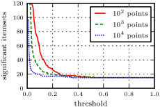
(a) Ind

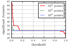
(b) Path

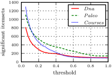
(c) Real datasets

Figure 2: Number of significant itemsets as a function of the threshold. The smallest threshold used for Ind and Path is $0.01$. The smallest threshold used for real datasets is $0.05$.

Ideally, for Ind, the dataset with independent variables we should have only $15$ significant itemsets, that is, the singletons, for any $\sigma>0$. Similarly, for Path we should have $15+14=29$ itemsets, the singletons and the pairs of form $a_{i}a_{i+1}$. We can see from Figures 2(a) and 2(b) that as we increase the number of transactions in data, the number of significant itemsets approaches these ideal cases, as predicted by Theorem 3.8. The convergence to the ideal case is faster in Path than in Ind. The reason for this can be explained by the curse of dimensionality. In Ind we have $15\times 14/2=105$ combinations of pairs of items. There is a high probability that some of these item pairs appear to be correlated. On the other hand, for Path, let us assume that we have the correct model. That is, the singletons and the $14$ pairs $a_{i}a_{i+1}$. The only valid itemsets of size $3$ that we can add to this model are of the form $a_{i}a_{i+1}a_{i+2}$. There are only $13$ of such sets, hence the probability of finding such itemset important is much lower. Interestingly, in Path we actually benefit from the fact that we are using decomposable models instead of general exponential models.

6.3 Use cases with real-world datasets

Our first experiment with real-world data is to study the number of significant itemsets as a function of the threshold $\sigma$. Figure 2(c) shows the number of significant itemsets for all three datasets. We see that the number of significant itemsets increases faster than for the synthetic datasets as the threshold decreases. The main reason for this difference, is that with real-world datasets we have more items and less transactions. This is seen especially in the Paleo dataset for which the number of significant itemsets increases steeply between the interval $0.4$–$1.0$ when compared to Dna and Courses.

Our next experiment is to compare the score against baselines, namely, the frequency $\mathit{fr}\mathopen{}\left(X\right)$ and entropy $H\mathopen{}\left(X\right)$. These comparisons are given in Figures 3(a) and 3(b). In addition, we computed the correlation coefficients (given in Table 2). From results, we see that $sc\mathopen{}\left(X\right)$ has a positive correlation with frequency and a negative correlation with entropy. The correlation with entropy is expected, since low-entropy implies that the empirical distribution of an itemset is different than the uniform distribution. Hence, using the frequency of such an itemset should improve the model and consequently the itemset is considered interesting.

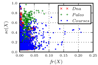
(a) score as a function of frequency

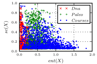
(b) score as a function of entropy

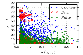
(c) index difference vs. score

Figure 3: Score $sc\mathopen{}\left(X\right)$ as a function of different baselines. In Figures 3(a) and 3(b) score is plotted as a function of frequency $\mathit{fr}\mathopen{}\left(X\right)$ and entropy $H\mathopen{}\left(X\right)$, respectively. In Figure 3(c) the difference between the largest index and the smallest index of an item is plotted as a function of $sc\mathopen{}\left(X\right)$. Singletons and itemsets with $sc\mathopen{}\left(X\right)<0.05$ are ignored. Additionally, only itemsets of size $2$ are used in Figure 3(c).

Data	$\mathit{fr}\mathopen{}\left(X\right)$	$H\mathopen{}\left(X\right)$	index diff.
Dna	0.16	-0.27	-0.28
Paleo	0.45	-0.16	-0.17
Courses	0.18	-0.35	-0.02

Table 2: Correlations of $sc\mathopen{}\left(X\right)$ and baselines.

Both datasets Paleo and Dna have a natural order between the items, for example, for Paleo dataset it is the era when particular species was extant. Our next experiment is to test whether this order is represented in the discovered patterns. In our experiments, the items in these datasets were ordered using this natural order. Let $X=a_{i}a_{j}$ be an itemset of size $2$. In Figure 3(c), we plotted $j-i$ as a function of $sc\mathopen{}\left(X\right)$. We used only itemsets of size $2$, since larger itemsets have inherently smaller scores and larger difference between the indices. In addition, we compute the correlation coefficients (given in Table 2). From the results we see that for Paleo and Dna the more significant itemsets tend to have a smaller difference between their indices. On the other hand, we do not discover any significant correlation in Courses.

Finally, we report some of the discovered patterns from Courses. The $4$ most significant itemsets of size $2$ are (Computer Architectures, Performance Analysis) with a score of $0.95$, (Design & Analysis of Algorithms, Principles of Functional Programming) scoring $0.94$, (Database Systems II, Information Storage) scoring $0.94$, (Three concepts: probability, Machine Learning) scoring $0.92$.

7 Conclusions

In this paper we introduced a novel and general approach for ranking itemsets. The idea behind the approach is to connect statistical models and collections of itemsets. This connection enables us to define the score of an itemset as the probability of itemset occurring in a random model. Doing so, we transformed the problem of mining patterns into a more classical problem of modeling.

As a concrete example of the framework, we used exponential models. These models have many important theoretical and practical properties. The connection with itemsets is natural and the Occam’s razor inherent to these models can be used against the pattern explosion problem. Our experiments support the theoretical results and demonstrate that the measure works in practice.

8 Acknowledgments

Nikolaj Tatti is funded by FWO postdoctoral mandate.

Appendix A Proofs for Section 3

Proof A.26 (of Theorem 3.7).

We will prove the theorem using the well-known connection between maximum entropy principle and exponential models. Let $q_{D}$ be the empirical distribution of the data. Let $\mathcal{P}$ be the collection of distributions,

$$\mathcal{P}=\left\{p\mid p(X=1)=\mathit{fr}\mathopen{}\left(X\right)=q_{D}(X=1),X\in\mathcal{F}\right\},$$

that is, a distribution in $\mathcal{P}$ has the same itemset frequencies for $\mathcal{F}$ as the data. Assume for the time being that all entries in $q_{D}$ are positive. Then, A well-known theorem [6] states that the unique distribution, say $p^{*}$, maximizing the entropy among $\mathcal{P}$ belongs to the exponential model $M$ such that $\mathit{fam}\mathopen{}\left(M\right)=\mathcal{F}$. Let the corresponding parameters for the model be $r^{*}$.

We need to show that $p^{*}$ is actually a maximum likelihood distribution. To see this, let $q\in M$ be another distribution from the model and let $r$ be its parameters. A straightforward calculus reveals that

$$\begin{split}\log\frac{p^{*}\mathopen{}\left(D\right)}{q\mathopen{}\left(D\right)}&=\sum_{t\in D}\log\frac{p^{*}(t)}{q(t)}\\ &={\left|D\right|}\sum_{t\in\left\{0,1\right\}^{K}}q_{D}(t)\log\frac{p^{*}(t)}{q(t)}\\ &={\left|D\right|}\sum_{t\in\left\{0,1\right\}^{K}}\sum_{X\in\mathcal{F}}q_{D}(X=1)(r^{*}_{X}-r_{X})\\ &={\left|D\right|}\sum_{t\in\left\{0,1\right\}^{K}}\sum_{X\in\mathcal{F}}p^{*}(X=1)(r^{*}_{X}-r_{X})\\ &={\left|D\right|}\sum_{t\in\left\{0,1\right\}^{K}}p^{*}(t)\log\frac{p^{*}(t)}{q(t)}\\ &={\left|D\right|}\mathit{KL}\mathopen{}\left(p^{*}\|q\right)\geq 0,\end{split}$$

where $\mathit{KL}\mathopen{}\left(p\|q\right)$ is the Kullback-Leibler divergence between $p^{*}$ and $q$. The inequality shows that $r^{*}$ has the highest likelihood. If $q_{D}$ has zero probabilities, then we can consider a sequence $\epsilon_{n}\to 0$ as $n\to\infty$. Define $q_{n}=(1-\epsilon_{n})q_{D}+\epsilon_{n}2^{-K}$. Let $p^{*}_{n}$ be the maximal entropy distribution computed from $q_{n}$. It is easy to show that a limit distribution of any converging subsequence of $p^{*}_{n}$ has the maximal entropy among $\mathcal{P}$. Since maximal entropy distribution is unique, the sequence $p^{*}_{n}$ converges to the unique value, say $p^{*}$. Following the same calculus as above we can show that $p^{*}$ is the maximal likelihood distribution

$$\begin{split}&\sum_{t\in\left\{0,1\right\}^{K}}q_{D}(t)\log\frac{p^{*}(t)}{q(t)}\\ &\qquad=\lim_{n\to\infty}\sum_{t\in\left\{0,1\right\}^{K}}q_{n}(t)\log\frac{p^{*}_{n}(t)}{q(t)}\\ &\qquad=\lim_{n\to\infty}\sum_{t\in\left\{0,1\right\}^{K}}\sum_{X\in\mathcal{F}}q_{n}(X=1)(r^{*}_{X}-r_{X})\\ &\qquad=\lim_{n\to\infty}\sum_{t\in\left\{0,1\right\}^{K}}\sum_{X\in\mathcal{F}}p^{*}_{n}(X=1)(r^{*}_{X}-r_{X})\\ &\qquad=\lim_{n\to\infty}\sum_{t\in\left\{0,1\right\}^{K}}p^{*}_{n}(t)\log\frac{p^{*}_{n}(t)}{q(t)}\\ &\qquad=\sum_{t\in\left\{0,1\right\}^{K}}p^{*}(t)\log\frac{p^{*}(t)}{q(t)}=\mathit{KL}\mathopen{}\left(p^{*}\|q\right)\geq 0.\end{split}$$

Finally, as the number of transactions goes into infinity $r^{*}$ converges to the true parameters of the model and $p^{*}$ converges into true underlying distribution $p$.

To prove Theorem 3.8 we will need the following lemma whose prove can be found for example in [21].

Lemma A.27.

Assume that $D$ with $N$ data points comes from a model $M$ with parameters $r$. Let $r^{N}$ be the maximal likelihood estimate. Then

$$\log P(D\mid M,r^{N})-\log P(D\mid M,r)$$

converges uniformly to $\chi^{2}$ distribution with $d\leq{\left|F\right|}-1$ number degrees of freedom.

Proof A.28 (of Theorem 3.8).

Let $M^{\prime}\neq M$ be a model and $\mathcal{F}^{\prime}=\mathit{fam}\mathopen{}\left(M^{\prime}\right)$. We need to show that

$$\frac{P(M^{\prime}\mid D)}{P(M\mid D)}\to 0$$

as the number of data points goes to infinity.

We will use the BIC estimate given in Eq. 3 to prove the theorem. Let $N={\left|D\right|}$. Let us define $p^{N}$ to be the maximal likelihood distribution from $M$ and $q^{N}$ to be the maximal likelihood distribution in $M^{\prime}$. Let us write

$$A_{N}=\log q^{N}(D)-\log p^{N}(D)$$

and

$$B_{N}=\log N({\left|\mathcal{F}\right|}-{\left|\mathcal{F}^{\prime}\right|})/2.$$

Then asymptotically

$$\log P(M^{\prime}\mid D)-\log P(M\mid D)=A_{N}+B_{N}.$$

Let $A$ be the limit of $A_{N}$ and $B$ be the limit of $B_{N}$.

Assume that $p\notin M^{\prime}$. Let $q\in M^{\prime}$ be the maximum likelihood distribution as $N\to\infty$. Since the exponential models are closed sets $q$ cannot be $p$. A straightforward calculation reveals that $N^{-1}A_{N}\to-\mathit{KL}\mathopen{}\left(p\|q\right)<0$. In addition, $N^{-1}B_{N}\to 0$. Thus $N^{-1}(A_{N}+B_{N})$ approaches a negative value, and so $A+B=-\infty$.

Assume that $p\in M^{\prime}$, then the conditions imply that ${\left|\mathcal{F}^{\prime}\right|}>{\left|\mathcal{F}\right|}$ so that $B=-\infty$. Lemma A.27 implies that $A$ is a difference of two $\chi^{2}$ distributions. More importantly, since convergence in Lemma A.27 is uniform we can compute the limit inside the probability so that the probability

$$P(A_{N}+B_{N}>\sigma)\to P(A+B>\sigma)=P(A>\infty)=0$$

for any $\sigma\in$. Hence $A_{N}+B_{N}$ approaches $-\infty$. This proves the theorem.

Proof A.29 (of Theorem 3.10).

Let $p(A)=P(A\mid M,r)$ be the distribution from a model $M$ with parameters $r$. To ease the notation, let us define $\mathcal{G}=\max\mathopen{}\left(\mathcal{F}\right)$ and

$$\mathcal{S}=\left\{X\cap Y\mid(X,Y)\in E(\mathcal{T})\right\}.$$

A classic result states that we can decompose $p$ to factors,

$$p(A=t)=\frac{\prod_{X\in\mathcal{G}}p(X=t_{X})}{\prod_{S\in\mathcal{S}}p(S=t_{S})},$$

where $t_{X}$ is a projection of a binary vector $t$ to the variables of $X$. Let $q(A)$ be the empirical distribution. Let $p$ be the maximum-likelihood distribution. The proof of Theorem 3.7 states that $p(X=1)=q(X=1)$ for any itemset $X\in\mathcal{F}$. Using the exclusion-inclusion rules and the fact that $\mathcal{F}$ is downward closed we can show that $p(X=t)=q_{D}(X=t)$ for every $X\in\mathcal{F}$ and every possible binary vector $t$ of length ${\left|X\right|}$. The log-likelihood is equal to

$$\begin{split}\log\prod_{t\in D}p(A=t)=&\sum_{t\in D}\log\frac{\prod_{X\in\mathcal{G}}p(X=t_{X})}{\prod_{S\in\mathcal{S}}p(S=t_{S})}\\ =&\sum_{X\in\mathcal{G}}\sum_{t\in D}\log p(X=t_{X})\\ &\ -\sum_{S\in\mathcal{S}}\sum_{t\in D}\log p(S=t_{S}))\\ =&{\left|D\right|}\sum_{X\in\mathcal{G}}\sum_{t_{X}}q(X=t_{X})\log p(X=t_{X})\\ &\ -{\left|D\right|}\sum_{S\in\mathcal{S}}\sum_{t_{S}}q(S=t_{S})\log p(S=t_{S}))\\ =&{\left|D\right|}\sum_{X\in\mathcal{G}}\sum_{t_{X}}q(X=t_{X})\log q(X=t_{X})\\ &\ -{\left|D\right|}\sum_{S\in\mathcal{S}}\sum_{t_{S}}q(S=t_{S})\log q(S=t_{S}))\\ =&-{\left|D\right|}\sum_{X\in\mathcal{G}}H\mathopen{}\left(X\right)+{\left|D\right|}\sum_{S\in\mathcal{S}}H\mathopen{}\left(S\right).\\ \end{split}$$

This proves the theorem.

Appendix B Proofs for Section 4

We will need the following technical lemma for several subsequent proofs.

Lemma B.30.

Let $X_{1},\ldots,X_{N}\in\max\mathopen{}\left(\mathcal{F}\right)$ with $N\geq 3$. Define $S_{i}=X_{i}\cap X_{i+1}$ and $S_{N}=X_{N}\cap X_{1}$. If each $S_{i}$ has a unique item (when compared to other $S_{i}$), then $\mathcal{F}$ is not decomposable.

Proof B.31 (of Theorem 4.13).

Let us assume that $X$ is the only itemset containing $x$ and $y$ simultaneously. Let $\mathcal{T}$ be a junction tree. The adjacent itemsets of $X$ either miss $x$ or $y$ or both. Thus we can remove $X$ and replace it $X-x$ and $X-y$, connected to each other, the adjacent itemsets of $X$ can be connected to either $X-x$ or to $X-y$. If $X-x$ is not maximal, that is there is an itemset $Z\supset X-x$ , then we can remove $X-x$ and connect all the edges going to $X-x$ to $Z$. We can repeat this for $X-y$ as well. The resulting tree is a junction tree.

To prove the other direction, assume that there is an another itemset $Y$ containing $x$ and $y$, simultaneously. There must be an item $z\in X$ such that $z\notin Y$. Then itemsets $Y$, $X-x$, and $X-y$ satisfy the requirements of Lemma B.30, hence the new family is not decomposable.

Proof B.32 (of Theorem 4.16).

Let $\mathcal{T}$ be a junction tree. Assume that $V$ and $W$ exist. By construction of $\mathit{rf}\mathopen{}\left(\mathcal{F};S\right)$ it follows that there must be two itemsets $X,Y\in\mathcal{F}$ such that $S=X\cap Y$, $x\in X$, and $y\in Y$. If $X$ and $Y$ are adjacent in $\mathcal{T}$, we can add $Z$ between $X$ and $Y$ (possibly removing $X$ and $Y$ if they are no longer maximal), and $\mathcal{T}$ still remains a junction tree.

If $X$ and $Y$ are not adjacent, then there is a path $P$ connecting them. There must be itemsets $P_{i}$ and $P_{i+1}$ along that path such that $P_{i}\cap P_{i+1}=S$, otherwise $X$ and $Y$ would have been merged during the construction of reduced family, which is a contradiction. If we remove edge $(P_{i},P_{i+1})$ and add edge $(X,Y)$ we will obtain an alternative junction tree for $\mathcal{F}$. It is straightforward to see that this tree is truly a junction tree. But in this tree $X$ and $Y$ are adjacent, so we can add $Z$ between them.

To prove the other direction, assume that adding $Z$ is a legal merge. By definition it immediately implies that there are sets $V,W\in\mathit{rf}\mathopen{}\left(\mathcal{F};S\right)$ such that $x\in V$ and $y\in W$. We need to show that $V\neq W$. Let $\mathcal{H}$ be the family resulted from the merge. Let $\mathcal{U}$ be a junction tree for $\mathcal{H}$. Let $X\in\max\mathopen{}\left(\mathcal{F}\right)$ be an itemset such that $S\cup\left\{x\right\}\subseteq X$ and, similarly, let $Y\in\max\mathopen{}\left(\mathcal{F}\right)$ such that $S\cup\left\{y\right\}\subseteq Y$. We may assume that $X\neq S\cup\left\{x\right\}$ and $Y\neq S\cup\left\{y\right\}$, otherwise the proof is trivial. Hence, $X,Y\in\max\mathopen{}\left(\mathcal{H}\right)$ Let $P$ be a path in $\mathcal{U}$ from $X$ to $Y$. Let $R$ be a path in $\mathcal{U}$ from $Z$ to $X$ and let $P_{e}$ be the first entry in path $R$ that also occurs in $P$. We must have $Z\cap X\subseteq P_{e}$. The path from $Z$ to $Y$ must also contain $P_{e}$, and so $Z\cap Y\subseteq P_{e}$. This implies that $Z=(Z\cap X)\cup(Z\cap Y)\subseteq P_{e}$. Since $Z$ is a maximal set, we must have $Z=P_{e}$.

Itemset $Z$ is the only maximal itemset in $\mathcal{H}$ that contains $x$ and $y$ simultaneously. Otherwise, Theorem 4.13 states that $\textsc{Split}\mathopen{}\left(Z,x,y\right)$ is illegal in $\mathcal{H}$ so $\textsc{Merge}\mathopen{}\left(S,x,y\right)$ is illegal in $\mathcal{F}$.

We can remove $Z=P_{e}$ from $\mathcal{U}$, attach $P_{e-1}$ and $P_{e+1}$ to each other, and connect the rest adjacent nodes either to $P_{e-1}$ or to $P_{e+1}$ depending whether these nodes have $x$ or $y$ as a member. The outcome, say $\mathcal{R}$, is a junction tree for $\mathcal{F}$.

If $V=W$, then there must be a sequence

$$X=\left(T_{1},\ldots,T_{N}\right)=Y\in\mathcal{F}$$

such that $S\subsetneq T_{i}\cap T_{i+1}$. Now consider a path $O$ in $\mathcal{R}$ visiting each $T_{i}$ in turn. Since $\mathcal{R}$ is a junction tree we must have $S\subsetneq O_{i}\cap O_{i+1}$. Since $X=T_{1}$ and $Y=T_{N}$ path $O$ must use the edge $(P_{e-1},P_{e+1})$. But we must have $P_{e-1}\cap P_{e+1}=S$, otherwise $\mathcal{U}$ would not have been a junction tree. This contradiction implies that $V\neq W$.

Proof B.33 (of Theorem 4.18).

We will prove the theorem by showing that all models can be brought by legal splits to the indepenence model. Since a split $\textsc{Split}\mathopen{}\left(X,x,y\right)$ and a merge $\textsc{Merge}\mathopen{}\left(X-\left\{x,y\right\},x,y\right)$, are the opposite operations we can reach model $M$ from $M^{\prime}$ by first reaching the independence model with splits and then reaching $M$ from the independence model by merges.

Let $\mathcal{T}$ be a junction tree for $\mathcal{F}^{\prime}=\mathit{fam}\mathopen{}\left(M^{\prime}\right)$ and let $X\in\max\mathopen{}\left(\mathcal{F}^{\prime}\right)$ be a maximal itemset such that $X$ is the leaf clique in a junction tree $\mathcal{T}$ with ${\left|X\right|}\geq 2$. If no such $X$ exist, then $M^{\prime}$ is in fact the independence model. Let $Y$ be the maximal itemset into which $X$ is connected in $\mathcal{T}$.

There must be an item $x\in X$ such that $x$ is not contained in any other maximal itemset of $\mathcal{F}^{\prime}$. To prove this, assume otherwise. Then for each item $z$ there is a maximal itemset $Z$ that contains $z$. The path from $X$ to $X$ must go through $Y$ so the running intersection property implies that $x\in Y$. But this implies that $X\subseteq Y$ which contradicts the maximality of $X$. Let $y\in X$ such that $x\neq y$. Theorem 4.13 now states that $\textsc{Split}\mathopen{}\left(X,x,y\right)$ is a legal operation. We can now iteratively apply this step until we reach the independence model. This proves the theorem.

Proof B.34 (of Theorem 4.19).

For notational convinience, let us write

$$a(M)=\sum_{(X,Y)\atop\in E(\mathcal{T})}H\mathopen{}\left(X\cap Y\right)\text{ and }b(M)=\sum_{X\in\max\mathopen{}\left(\mathcal{F}\right)}H\mathopen{}\left(X\right).$$

Theorem 3.10 and Eq. 3 implies that

$$\log A={\left|D\right|}\mathopen{}\left(a(M)-b(M)\right)-\frac{\log{\left|D\right|}({\left|\mathcal{F}\right|}-1)}{2}$$

and

$$\log B={\left|D\right|}\mathopen{}\left(a(M^{\prime})-b(M^{\prime})\right)-\frac{\log{\left|D\right|}({\left|\mathcal{F}^{\prime}\right|}-1)}{2}.$$

Let us write $d={\left|D\right|}(a(M^{\prime})-b(M^{\prime})-a(M)+b(M))$. We will first show that $d=\mathit{gain}\mathopen{}\left(X,x,y\right)$. Let us denote $S=X-\left\{x,y\right\}$, $U=X-x$, and $V=X-y$. Consider the possibility that $U$ is not maximal in $\mathcal{F}^{\prime}$, in such case there must be a maximal itemset $Q\in\mathcal{F}$ such that $U\subset Q$ and that $Q$ is adjacent to $X$ with a separator $U$. Similarly, if $V$ is not maximal in $\mathcal{F}^{\prime}$, then there is a maximal itemset $P\in\mathcal{F}$ such that $V\subset P$ and that $P$ is adjacent to $X$ with a separator $V$. By studying the first part of the proof of Theorem 4.13 we see that there are four possible cases depending whether $U$ and/or $V$ is maximal set in $\mathcal{F}^{\prime}$. The split operations are

(Case 1)

(Case 2)

(Case 3)

(Case 4)

In all cases, the difference $d$ is equal to $H\mathopen{}\left(X\right)+H\mathopen{}\left(S\right)-H\mathopen{}\left(V\right)-H\mathopen{}\left(U\right)=\mathit{gain}\mathopen{}\left(X,x,y\right)$. For example, in Case 2, the term $H\mathopen{}\left(X\right)$ is in $b(M)$ but not in $b(M^{\prime})$, similarly the term $H\mathopen{}\left(U\right)$ is in $b(M^{\prime})$ but not in $b(M)$, consequently $b(M)-b(M^{\prime})=H\mathopen{}\left(X\right)-H\mathopen{}\left(U\right)$. Similarly, $a(M)-a(M^{\prime})=H\mathopen{}\left(V\right)-H\mathopen{}\left(S\right)$. Thus $d=\mathit{gain}\mathopen{}\left(X,x,y\right)$ for Case 2, and similar observations show that $d=\mathit{gain}\mathopen{}\left(X,x,y\right)$ holds also for other cases.

To complete the proof we need to show that ${\left|\mathcal{F}\right|}-{\left|\mathcal{F}^{\prime}\right|}=2^{{\left|X\right|}-2}$. During a split, itemsets containing $x$ and $y$ are removed, but there are exactly $2^{{\left|X\right|}-2}$ such itemsets. We can now combine these results

$$\begin{split}\log B-\log A&=d-\frac{\log{\left|D\right|}}{2}({\left|\mathcal{F}\right|}-{\left|\mathcal{F}^{\prime}\right|})\\ &=\mathit{gain}\mathopen{}\left(X,x,y\right)-\log{\left|D\right|}2^{{\left|X\right|}-3},\\ \end{split}$$

which proves the theorem.

Proof B.35 (of Theorem 4.20).

Let $X_{i}$ and $Y_{i}$ be the maximal itemsets such that $X_{i}\cap Y_{i}=S_{i}$, $x_{i}\in X_{i}$ and $y_{i}\in Y_{i}$. These sets must exist since adding $Z_{i}$ is a legal merge.

Assume that $Z_{1}=Z_{2}$. This implies that either all items $x_{1}$, $y_{1}$, $x_{2}$, and $y_{2}$ are unique or two of them are the same. Assume the latter case and assume that $x_{1}=x_{2}$. Then we must have $y_{2}\in S_{1}-S_{2}$ and $y_{1}\in S_{2}-S_{1}$. We have $x_{1}\in X_{1}\cap X_{2}$, $y_{1}\in X_{2}\cap Y_{1}$, and $y_{2}\in Y_{1}\cap X_{1}$. Hence the conditions in Lemma B.30 hold and $\mathcal{F}$ is not decomposable.

Assume now that all four items are unique. This implies that $x_{1},y_{1}\in S_{2}-S_{1}$ and $y_{2}\in S_{1}-S_{2}$. Again we have $x_{1}\in X_{1}\cap X_{2}$, $y_{1}\in X_{2}\cap Y_{1}$, and $y_{2}\in Y_{1}\cap X_{1}$ so Lemma B.30 implies that $\mathcal{F}$ is not decomposable.

Proof B.36 (of Theorem 4.21).

Let $S$ be an itemset. We will show that $\mathit{md}\mathopen{}\left(M,S\right)>0$ only if $S$ is a separator, that is, $S=X\cap Y$ for two adjacent itemsets in a junction tree. The theorem will follow from this, since a junction tree contains at most $K$ nodes and hence at most $K-1$ edges.

To prove the result, assume that $\mathit{md}\mathopen{}\left(M,S\right)>0$. This implies that there are two sets, say $U,V\in\mathit{rf}\mathopen{}\left(\mathcal{F},S\right)$. Let $x\in U$ and $y\in V$. This implies that there are (at least) two sets $X$ and $Y$ such that $S\cup\left\{x\right\}\subset X$ and $S\cup\left\{y\right\}\subset Y$. Let $P=\left(P_{1},\ldots,P_{L}\right)$ be a path from $X$ to $Y$ in the junction tree. The running intersection property implies that $S\subseteq P_{i}\cap P_{i+1}$ If there is no $i$ such that $S=P_{i}\cap P_{i+1}$, then $X$ and $Y$ should have been joined together during the construction of $\mathit{rf}\mathopen{}\left(\mathcal{F},S\right)$. In other words, there must be a set in $\mathit{rf}\mathopen{}\left(\mathcal{F},S\right)$ containing $x$ and $y$. Hence, there are adjacent itemsets $P_{i}$ and $P_{i+1}$ such that $S=P_{i}\cap P_{i+1}$. This proves the theorem.

Proof B.37 (of Theorem 4.22).

Adding $X=S\cup\left\{x,y\right\}$ into $\mathcal{F}$ can only make splits illegal. Assume that $\textsc{Split}\mathopen{}\left(Y,a,b\right)$ becomes illegal after adding $X$. Theorem 4.13 implies that $a,b\in X$. We must have $\left\{a,b\right\}\not\subseteq S$ since otherwise the split would not be legal in the original family. Assume that $a=x$ and let $W\in\max\mathopen{}\left(\mathcal{F}\right)$ is the maximal itemset containing $\left\{x\right\}\cup S$ (such itemset exists because of the definition of merge). Note that, $b\neq y$, so $b\in S$ and $\left\{a,b\right\}\in W$. If there is another maximal itemset, say $Z\in\max\mathopen{}\left(\mathcal{F}\right)$, such that $\left\{x,b\right\}=\left\{a,b\right\}\subset Z$, then the split $\textsc{Split}\mathopen{}\left(Y,x,b\right)$ is not legal in the original family. This proves the theorem.

Proof B.38 (of Theorem 4.23).

Let $Z=S\cup\left\{x,y\right\}$. This itemset is the only maximal itemset in $\mathcal{G}$ that contains $x$ and $y$ simultaneously. The definition of reduced family now implies immediately Claims 2 and 3.

To prove Claim 1 let $V,W\in\mathit{rf}\mathopen{}\left(\mathcal{F};S\right)$ such that $x\in V$ and $y\in W$. These must be separate sets because of Theorem 4.20. The set $Z$ now connects these sets into one in $\mathit{rf}\mathopen{}\left(\mathcal{G};S\right)$.

To see Claim 4 let $T$ be an itemset. If $x,y\in T$, then $\mathit{rf}\mathopen{}\left(\mathcal{G};T\right)$ has only one set and $\mathit{rf}\mathopen{}\left(ifam{G};T\right)$ has zero sets. If $x\in T$ and $y\notin T$, then $T-S\neq\emptyset$, otherwise $T$ is covered by Claim 2 or 3. In such case, the construction of $\mathit{rf}\mathopen{}\left(\mathcal{G};T\right)$ does not use $Z$, and hence remains unchanged. Assume that $x,y\notin T$. Let $X,Y\in\max\mathopen{}\left(\mathcal{F}\right)$ be the itemsets such that $S\cup\left\{x\right\}\subseteq X$ and $S\cup\left\{y\right\}\subseteq Y$. If $T-S\neq\emptyset$, then $Z$ is not used. Assume now that $S\subsetneq T$. In this case the items of $X-T$ and $Y-T$ are already joined into one itemset, hence $\mathit{rf}\mathopen{}\left(\mathcal{G};T\right)$ remains unchanged.

References

- [1] C. C. Aggarwal and P. S. Yu. A new framework for itemset generation. In PODS ’98: Proceedings of the seventeenth ACM SIGACT-SIGMOD-SIGART symposium on Principles of database systems, pages 18–24. ACM Press, 1998.
- [2] R. Agrawal, H. Mannila, R. Srikant, H. Toivonen, and A. I. Verkamo. Fast discovery of association rules. In Advances in Knowledge Discovery and Data Mining, pages 307–328. AAAI/MIT Press, 1996.
- [3] S. Brin, R. Motwani, and C. Silverstein. Beyond market baskets: Generalizing association rules to correlations. In J. Peckham, editor, SIGMOD 1997, Proceedings ACM SIGMOD International Conference on Management of Data, pages 265–276. ACM Press, May 1997.
- [4] C. Chow and C. Liu. Approximating discrete probability distributions with dependence trees. IEEE Transactions on Information Theory, 14(3):462–467, 1968.
- [5] R. G. Cowell, A. P. Dawid, S. L. Lauritzen, and D. J. Spiegelhalter. Probabilistic Networks and Expert Systems. Statistics for Engineering and Information Science. Springer-Verlag, 1999.
- [6] I. Csiszár. I-divergence geometry of probability distributions and minimization problems. The Annals of Probability, 3(1):146–158, Feb. 1975.
- [7] M. Fortelius, A. Gionis, J. Jernvall, and H. Mannila. Spectral ordering and biochronology of european fossil mammals. Paleobiology, 32(2):206–214, March 2006.
- [8] S. Hanhijärvi, M. Ojala, N. Vuokko, K. Puolamäki, N. Tatti, and H. Mannila. Tell me something I don’t know: randomization strategies for iterative data mining. In Proceedings of the 15th ACM SIGKDD International Conference on Knowledge Discovery and Data Mining (KDD 2009), pages 379–388, 2009.
- [9] H. Heikinheimo, J. K. Seppänen, E. Hinkkanen, H. Mannila, and T. Mielikäinen. Finding low-entropy sets and trees from binary data. In Proceedings of the 13th ACM SIGKDD international conference on Knowledge discovery and data mining (KDD 2007), pages 350–359, 2007.
- [10] H. Heikinheimo, J. Vreeken, A. Siebes, and H. Mannila. Low-entropy set selection. In Proceedings of the SIAM International Conference on Data Mining (SDM 2009), pages 569–580, 2009.
- [11] S. Jaroszewicz and D. A. Simovici. Interestingness of frequent itemsets using bayesian networks as background knowledge. In KDD ’04: Proceedings of the tenth ACM SIGKDD international conference on Knowledge discovery and data mining, pages 178–186, New York, NY, USA, 2004. ACM.
- [12] R. Meo. Theory of dependence values. ACM Trans. Database Syst., 25(3):380–406, 2000.
- [13] S. Myllykangas, J. Himberg, T. Böhling, B. Nagy, J. Hollmén, and S. Knuutila. Dna copy number amplification profiling of human neoplasms. Oncogene, 25(55):7324–7332, Nov. 2006.
- [14] D. Pavlov, H. Mannila, and P. Smyth. Beyond independence: Probabilistic models for query approximation on binary transaction data. IEEE Transactions on Knowledge and Data Engineering, 15(6):1409–1421, 2003.
- [15] G. Schwarz. Estimating the dimension of a model. Annals of Statistics, 6(2):461–464, 1978.
- [16] A. Siebes, J. Vreeken, and M. van Leeuwen. Item sets that compress. In Proceedings of the SIAM International Conference on Data Mining (SDM 2006), 2006.
- [17] N. Tatti. Computational complexity of queries based on itemsets. Information Processing Letters, pages 183–187, June 2006.
- [18] N. Tatti. Maximum entropy based significance of itemsets. Knowledge and Information Systems, 17(1):57–77, 2008.
- [19] N. Tatti and H. Heikinheimo. Decomposable families of itemsets. In Knowledge Discovery in Databases: PKDD 2008, 11th European Conference on Principles and Practice of Knowledge Discovery in Databases, pages 472–487, 2008.
- [20] N. Tatti and J. Vreeken. Finding good itemsets by packing data. In Proceedings of the 8th IEEE International Conference on Data Mining (ICDM 2008), pages 588–597, 2008.
- [21] A. Wald. Tests of statistical hypotheses concerning several parameters when the number of observations is large. Transactions of the American Mathematical Society, 52(3):426–482, 1943.