Machine learning and chord based feature engineering for genre prediction in popular Brazilian music

Abstract

Music genre can be hard to describe: many factors are involved, such as style, music technique, and historical context. Some genres even have overlapping characteristics. Looking for a better understanding of how music genres are related to musical harmonic structures, we gathered data about the music chords for thousands of popular Brazilian songs. Here, ’popular’ does not only refer to the genre named MPB (Brazilian Popular Music) but to nine different genres that were considered particular to the Brazilian case. The main goals of the present work are to extract and engineer harmonically related features from chords data and to use it to classify popular Brazilian music genres towards establishing a connection between harmonic relationships and Brazilian genres. We also emphasize the generalisation of the method for obtaining the data, allowing for the replication and direct extension of this work. Our final model is a combination of multiple classification trees, also known as the random forest model. We found that features extracted from harmonic elements can satisfactorily predict music genre for the Brazilian case, as well as features obtained from the Spotify API. The variables considered in this work also give an intuition about how they relate to the genres.

Keywords feature engineering  $\cdot$ MIR  $\cdot$ random forests  $\cdot$ chords  $\cdot$ genre classification

1 Introduction

Many factors are involved in the configuration of a music genre: style, music techniques, historical context, regional identity, harmonic structures and so on [1]. A list of popular music genres can be easily found, but it usually does not come with no proper description for each one [2]. For the Brazilian case, some music genres even hold overlapping characteristics, making it harder to distinguish one from another. Musical genres facilitate the search for music, enveloping a simplification of what each song is. [3] found that users prefer to look for music of their interest by genre rather than by other metrics, such as artist similarity. Thereby, inconsistencies and blurriness in the definition of musical genres pose an important problem in various aspects of music studies.

Meanwhile, as [4] and [5] observed, mid-level music features such as chords configure a rich resource of information regarding genres. The chords sequence of a song fully describes its harmonic progression and, by consequence, represents a meaningful part of the total music structure. Therefore, the focus of this work is to establish a connection between harmonic information and genre specification in Brazilian popular music. Here, the term ’popular’ does not refer only to the genre named MPB, that stands for Música Popular Brasileira [6], or Brazilian Popular Music, but to nine genres that were considered familiar to the Brazilian context.

Musical data is available in a wide variety of formats for the genre classification task: music sheets, chords, lyrics, MIDI, audio files, and others [7]. Each one of those formats carries different levels of information about the pieces. The choice of a data format to work also defines what kind of information will be available for the analysis. The choice of symbolic chords data allows us to extract harmonically related features for the genre classification. More than just using raw information, we can capture deeper characteristics of the songs by representing their chords structures in different and meaningful forms.

Related work has been done for most of the usual representations of music data. For audio data, we can mention [8], [9], [10] and [11], all of which focused in music genre classification using audio extracted features. Concerning text data related to music, [12] presents a discussion about the characterization of genres through song lyrics. A recent interesting publication is [13], where the authors introduced a vector based representation for chords sequences. This work is notable in the sense that it brings to light a new and effective way to extract information about symbolic chords data. A similar problem to ours was attacked in [14], where the authors also focused on harmonic features for genre classification. However, only three musical genres were considered, while the role of chords in the classification was given only by its symbolic form, making it overly simplistic and leaving room for a better representation of the chords structures. Furthermore, in all of the mentioned, researchers did not focus neither on the manual extraction and consequent interpretation of the features or on extending the method used for the obtention of the data, which are the premises of our approach.

It is also important to notice that, until recent times, studies about popular music in Brazil were conducted typically by folklorists and musicians who worked mainly with classic Brazilian genres, such as Samba and Bossa Nova ([15], [16] and [17]). Music research was more focused on tradition and ethnic matters of Brazilian culture and their authenticity against foreign music. During the last few years, research in Brazilian popular music has become stronger and more inclusive concerning genres, but we still lack references when looking for works within the machine learning context. Recognizing that music information retrieval is an impactive study field [18], we see this as an opportunity to bring the two subjects together.

The main goals of the present work are to extract and engineer harmonically related features from chords data and use it to correctly classify popularly Brazilian music genres, towards establishing a connection between harmonic relationships and music genres. We also emphasize on the generalization of the method for obtaining the data, allowing for the replication and direct extension of this work. The following section describes how the data was obtained and analyzed, being complemented in Section 3 by the methods for the music genre modeling. We present the results regarding the construction of the variables, exploratory analysis and machine learning models applied in Section 4. Conclusions are in Section 5, containing a summary of the results, future work and final remarks about the project.

2 MATERIALS

A musical chord is a grouping of three or more notes played simultaneously [19]. There is usually a third interval between each note. When the chord is composed of three notes we have a triad, and when it has four notes, a tetrad. Triads are formed by a fundamental note, a third and a fifth note, being that a tetrad is different because it is added by a seventh note. These simple structures can be altered in many different ways, either by changing the current, removing or adding notes. Other nomenclatures rise depending on the change made, namely major, minor, augmented and diminished chords.

The same chords can have different tonal functions, which are determined by their positions (or degrees) in the underlying music scale of a song. For example, the C major chord is the first degree in the C scale, characterizing it as the tonic chord, the one that gives the human ear a sensation of closure. On the other hand, the C major chord has a totally different function when played within the F scale, where it assumes the dominant role and carries a tension feel.

Chords progressions are a sequence of chords that happen in a particular form. Some chords progressions have familiar patterns and it is well known in harmony theory that the occurrence of a chord is correlated to the previous one for a reason [19]. The most common case of this dependence is when a tension chord happens and it is followed by a resolution chord, giving the human ear a feeling of satisfaction after the tense moment. Even with the existence of patterns, those structures can actually be very diverse, inducing a wide range of sensations [20]. The way how a progression of chords is organized defines how the harmonics of a song is structured and different genres explore it in their own way.

2.1 Data Extraction

The data was extracted through webscraping techniques [21], from the Cifraclub website
(https://www.cifraclub.com.br/), an online collaborative Brazilian page of music-sharing. The website has a big collection of music chords for different instruments, and it is colaborative in the sense that most of the chords information present there are contributions of the users, what confers to the extracted data a natural high variability.

In total, nine music genres were used: Reggae, Pop, Forró, Bossa Nova, Sertanejo, MPB, Rock and Samba, chosen for being considered good representatives of the Brazilian music, since they are constantly present in the dynamic ’Top Brasil’ Spotify playlist [22]. Also, all of the nine genres appear on the main page of the Cifraclub website, where the most popular genres are. Other famous genres, as the Brazilian Funk and electronic music were, not evaluated as they can be better described by their percussion characteristics instead of the harmonics. From the selected genres, 106 different artists were available (solo singers or bands) on the Cifraclub platform.

Our extraction method consists of the access of the source code of each song for all the artists and, from the underlying html structures of the web pages, the collection of chords, keys, name of the artist and the name of the songs. Complementary variables about the release year and popularity were obtained with the aid of the Spotify API. We finished with a dataset of almost 484.000 rows related to 106 artists and 8339 different songs from the 9 Brazilian music genres.

To amplify the coverage of this work, the data extraction process resulted in the chorrrds package  [23], for the statistical software R [24]. The package is available for download and use from CRAN, the official repository of R packages. We point out that the creation of the package is especially beneficial for the reproducibility purposes of this analysis, and for ensuring that the method can be generalized and even extended.

2.2 Feature Engineering

One important step of modeling is feature engineering [25], that can directly influence the effectiveness of a statistical model. Feature engineering techniques are used when transformations of variables into features that represent the adjacent problem in a better way are needed [26], which depends on the context of the problem. The usefulness of the method for this work is explicit once the symbolic representation of chords progressions do not capture all of the possible useful information.

If we account for the chords in their simplest form, ignoring the possible alterations, it is noticeable that the same chord progressions inevitably turn up in some music genres, for example. Out of that, we consider that using only the raw information about the chords progression may cause a lot of information to be lost in the process. The details, such as if the chord was changed in some way or how prevalent they are in a song, should be taken into consideration. We emphasized on obtaining various distinct features from the chords, being able to make use of more information than only their symbolic form.

Feature engineering is typically automatic [26], meaning that the model learns the features without much human intervention. These features are hard to interpret or the interpretation is out of the scope of the research. Here, an opposite approach was employed, We chose to employ a hand-engineering approach to the variables, as we are interested in obtaining features that are interpretable in accordance to the posed problem. The resulting features will not only help with the modeling problem, but also have a clear interpretation of harmonic characteristics of the considered songs. In Table 1, a small demonstration of how the features were constructed is presented.

Table 1: Example of how features were manually extracted.

$$\begin{array}[]{|c|c|c|c|}chord&major&contain\thinspace 7th&contain\thinspace 6th\\ \hline\cr C&1&0&0\\ Gm7&0&1&0\\ \hline\cr\lx@intercol\hfil\hfil\lx@intercol&\lx@intercol\raisebox{6.0pt}{\hbox to0.0pt{$\quad\quad\underbrace{\hphantom{\mbox{$p\lor{}q$\hskip 55.4pt$p\land{}q$}}}_{extracted\thinspace features}$\hss}}\hfil\end{array}$$

The technique allowed us to have a dataset composed of 23 variables related to the songs, detailed in the next section of this paper. These features were divided into four thematic groups: triads (6), tetrads (6), common transitions (3) and miscellany (8). As the objective is not to model the songs but the music genres in which they are classified, the features went through a summarizing process. For example, consider the second column of Table 1. This column shows an indicator variable of the current chord being major or not. For each song, this column was turned into the percentage of major chords. The same was adequate for the last two columns of the example table. In this fashion, we summarized our extracted variables, ending up with one row of information per song.

3 MUSIC GENRE MODELING

In this section, we discuss how the variables were extracted and the method used for the music genre modeling.

3.1 Extracted and Engineered Variables

As mentioned before, one of our main concerns is that the new features can be interpretable. The engineered variables were separated into four thematic groups, organized as follows:

• First group - Triads and simple tetrads:

  1. Percentage of suspended chords (e.g. Gsus).

  2. Percentage of chords with the seventh (e.g. C7).

  3. Percentage of minor chords with the seventh (interaction between the minor third and the seventh) (e.g. Em7, C#m7).

  4. Percentage of minor chords (e.g. Em, C#m).

  5. Percentage of diminished chords (e.g. Bº).

  6. Percentage of augmented chords (e.g. Baug).

• Second group - Dissonant Tetrads:

  1. Percentage of chords with the fourth (e.g. D4).

  2. Percentage of chords with the sixth (e.g. E6).

  3. Percentage of chords with the ninth (e.g. G9).

  4. Percentage of minor chords with the major seventh (e.g. F7+, Am7+).

  5. Percentage of chords with a diminished fifth (e.g. C5- or C5b).

  6. Percentage of chords with as augmented fifth (e.g. C5+ ou C5#).

• Third group - Main Chord Transitions:

  1. Percentage of the first most common chord transition in the song.

  2. Percentage of the second most common chord transition in the song.

  3. Percentage of the third most common chord transition in the song.

• Fourth group - Miscellany:

  1. Popularity of the song, extracted from the Spotify API.

  2. Total of non-distinct chords in the song.

  3. Year of album release, extracted from the Spotify API.

  4. Indicator of the key of the song being the same as the most common chord.

  5. Percentage of chords with varying bass (e.g. C/E, C/G, C/Bb).

  6. Mean distance of the chords to the ’C’ chord in the circle of fifths.

  7. Mean distance of the chords to the ’C’ chord in semitones.

  8. Absolute quantity of the most common chord.

The first group contains information about small changes that can be done in the fundamental state of a chord. It captures when the song is the result of slight alterations in the chords. The second comprises more unusual extensions, commonly made by experienced musicians. By forming these groups of variables we can expect that if differences in harmonic structures between genres are really relevant, those characteristics would be pertinent to the harmonic characterization of the genres.

The set of transition variables is also organized with the intention of capturing the refinement of harmonic structures. For example, simplistic pieces tend to have a lesser variety of chords, but this does not mean that the songs last less time. This implies that the same group of chords and their transitions will be repeated many times for the whole duration of the song. In consequence, the top most common transitions would have high percentages, since there are not numerous different transitions happening in the song. A new dimension of complexity of the songs is mapped in this group of features.

The last group is a complete miscellany. It mixes very dissimilar predictors, possibly with distinct interpretations to the genres. We still have some features that concern the harmonic structures, in case they were not captured before, including the total of chords, the percentage of chords with varying bass and mean distances of the chord to the circle of fifths and by semitones. To explain a little, the first variable contains the information about the duration of the song, while the varying bass is also indicative of a more complex piece.

Besides that, in music theory relationships between chords can be measured with the circle of fifths [27]. To contextualize, this a circle that represents music chords, each one being a fifth apart from its neighbor. Usually, the neighbors appear together in a song, as their distance in a circle of fifths works as an indicator of their harmonic functions. For example, when the C chord is been played, it is very likely to be followed by the G, which is its adjacent neighbor in the circle of fifths [28]. We made use of this meaningful representation to obtain the distance features from our data. By calculating the mean distances in the circle of fifths for each song, we can estimate how the variations of chords happen in the selected songs. We already know from [29] that some pieces do not have highly varying progressions, while others experiment with particular combinations. As for the last features, the year has the temporal dimension and popularity is composed of the public opinion about the songs, which is as external element. These two last features were extracted from the Spotify API.

Starting only with the symbolic representation of the chords, we gathered a broad set of information about the considered pieces. A fundamental characteristic of this data is the interpretation behind each feature. Since one of our goals is to better understand how genres are related to musical harmony in general, the interpretation is a primary element of this work. The variables were complemented with selected features extracted from the Spotify API that carry important details.

3.2 Trees and Random Forests

First, consider a variable of interest $Y_{i}\in\mathbb{R}$ and $\mathbf{x}=(x_{i1},\dots,x_{ip})^{\prime}$ the set of predictor features, $1\leq i\leq p$. A statistical framework for non-parametric regression characterizes their relationship as

$$y_{i}=f_{0}(\mathbf{x_{i}})+\epsilon_{i},\thinspace\epsilon_{i}\stackrel{{\scriptstyle iid}}{{\sim}}N(0,\sigma^{2}),$$ (1)

where $f_{0}$ is an unknown regression function. A regression tree is a completely non-parametric model, described graphically by a tree, that can be used to reconstruct $f_{0}$ by mapping the predictors into a set of decisions at each step. On the literature, trees are applied in decision problems where there is no stochastic assumption made, but instead, there is interest in finding rules that would lead to the right predictions [30]. Each rule has the form: $x_{j}>x_{j,th}$, where $x_{j}$ describes the value of the feature at $j$ and $x_{j,th}$ is the decision cut point [31]. For the purpose of explaining how the trees work, consider a classification task for a factor target variable. In our case, this factor variable is the music genres. At the start, the full training dataset is all in just one node of the tree. In each step of the algorithm, a binary partition is made in the covariables space, meaning that a split results in two children that separate better the target variable in its classes. The usual criteria to choose the best threshold for a new node is the Gini impurity [32], measured by

$$Gini=1-\sum_{c=1}^{r}p_{c}^{2},$$ (2)

where $p_{c}$ is the observed proportion for each class $c=1,..r.$ in the dataset. This measure has its minimum when the individuals belong to the same class. Thereby, partitions are made in order to minimize the difference between the impurity, or heterogeneity, of the current state of the model and the next step with the candidate new node. This difference is written as

$$\Delta Imp=Imp_{O}-\Big{(}\frac{n_{1}}{n_{O}}Imp_{1}+\frac{n_{2}}{n_{O}}Imp_{2},\Big{)}$$ (3)

where $1$ e $2$ are the candidate divisions, starting at region $O$. Consequently, the algorithm looks for the splitting cut point that leads to the minimal combined impurity of the groups.

There exist a few advantages of the use of trees. Non-linear decision regions between the covariables are better captured by this algorithm than with usual regression models. Consider Figure 1 as an example: a linear model would not be able to reproduce the relationship between the two variables very well. As we see in Figure 2, a tree model with the decision rules configured as the gray lines displayed, on the other hand, would satisfactorily separate the observations in the two existing classes.

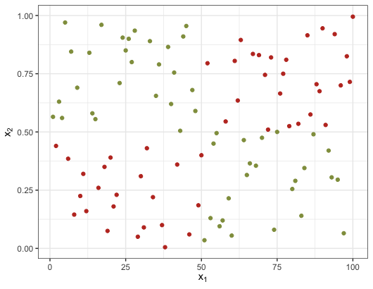
Figure 1: Two covariables with the target variable groups mapped in the color of the points.

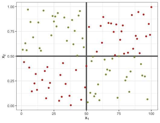
Figure 2: Exemplification of the decision rules that would separate the two groups well.

The performance of the tree algorithm needs to be evaluated regarding its prediction power. A test set is generally used to produce the predictions for never seen data. The comparison is performed between what was observed for the test set and what the tree model predicts. The closer the predictions are to the vector of observations, the better the algorithm is doing, and an accuracy measure is calculated as

$$Acc=\frac{1}{n}\sum_{i=1}^{n}I(y_{i}\neq\hat{y}_{i})$$ (4)

where $I$ is the indicator for whether the model prediction $\hat{y}_{i}$ is compatible with what was observed and $n$ is the sample size [32].

Once we defined decision trees, we can extend the definition to the random forest algorithm. A random forest is an ensemble learning algorithm introduced by Breiman [33], that works by constructing a large number $B$ of trees and combining their results [32]. For each tree, a bootstrapped dataset [34] and only a set of $m$ predictors, from the $p$ total, are considered. Typically, the variables are selected randomly for each step of the algorithm and $m$ is chosen as approximately $\sqrt{p}$ [32].

Since the correlation between the trees can be an issue, selecting just a few variables for each step is useful to overcome this problem [35]. If the trees are allowed to consider different variables at each time, strong predictors will not dominate the algorithm, as sometimes they will not be even available for the split. Using this criterion, the results produced by the uncorrelated trees are more reliable [32]. The final prediction for the random forest classification algorithm is the majority vote of the $B$ trees or, in other words, the classification proposed by most of the trees is the one that will be taken as the prediction of the final model.

3.3 Genre Modeling

The nine music genres present in our dataset were modeled with a random forest algorithm. Our target variable is the music genres, while the predictors are the extracted and engineered features. In total, four models were fitted, in a nested fashion, structured as

1. First model: triads (6)

2. Second model: triads (6) + tetrads (6)

3. Third model: triads (6) + tetrads (6) + common transitions (3)

4. Fourth model: triads (6) + tetrads (6) + common transitions (3) + miscellany (8).

Our first model accounted for the first six variables, related to the triad features of the chords. The following model was added the tetrads variables and the third model was built using also the common transitions variables. Lastly, the fourth model also considered the miscellany variables, adding up to 23 predictors. In this way, we could compare the predictions for all the different four models. The interest relied on assess the information brought by each thematic group of predictors.

4 RESULTS

In this section, we present a summary of the exploratory analysis along with the results of the fitted models. The discussion is shown in the following section.

4.1 Exploratory Analysis

Non-linearity between predictor variables is not an assumption of the random forest model, but rather a problem that the algorithm can overcome. Nevertheless, Figures 3, 4 and 5 illustrate the the relationship between some variables of the first group. It is clear that the relationships between the variables follow a diversity of patterns between the music genres. With the plots, we can notice that the patterns would be poorly described if a linear function was considered for this task, as there is evidence of non-linear relationships in our dataset.

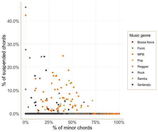
Figure 3: Percentage of minor chords in the song versus the percentage of suspended chords, identifying the music genre.

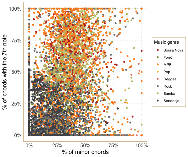
Figure 4: Percentage of minor chords in the song versus the percentage of chords with the seventh note, identifying the music genre.

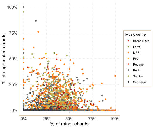
Figure 5: Percentage of minor chords in the song versus the percentage of augmented chords, identifying the music genre.

In addition to that, it has become common sense to say that some music genres are harmonically simpler than others [19]. We established as a diversity measure the mean of the count of distinct chords, obtained per song for each genre. Figure 6 shows how this mean behaves and has changed over the years for the genres (1957 to 2018). Clearly, genres known as traditionally Brazilian, like Samba, MPB, and Bossa Nova, have higher values of the mean count of distinct chords. These genres also have a higher variation over time, which is in agreement with popular knowledge [1]. Bossa Nova is the most unstable one, having different values along the years with an increasing trend, followed by Samba, that also looks to have been going through similar changes. Sertanejo is the one that has the most evident decrease, having a peak around 2000 and decay since that. The remaining genres are more harmonically uniform and stable through time. We also observe that data is not available for all of the years and genres, once some genres just appeared in Brazil in recent years [1].

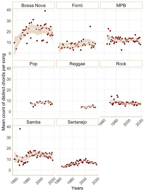
Figure 6: Mean count of distinct chords in the songs for each year, by music genre. The white curve represents a local regression non-parametric smoother to highlight the trend of the observations.

4.2 Random Forests Models

The random forest model was chosen as the classification algorithm for the music genres. All of the final variables were used in the modeling. Our choice for this algorithm is justified by three main points:

• it easily allows the obtention of an importance measure of the predictors,

• there is no need to normalize or transform the variables, once the trees are invariant to the predictor’s scale,

• accommodation of non-linear relationships between the predictors and the response, which are overcome by the model.

The full dataset was randomly partitioned in train  (70%) and test  (30%) set, with balancing by music genre. The train set was used for the training of the model, while the test set serves for the calculation of performance measures in data not seen by the trained model. Table 2 presents the structure of the two datasets and the measures of goodness of fit of the four models are in Table 3

Table 2: Amount of songs for each genre, in each partition, and representation (%) of the genre in the full dataset.

Genre	Train	Test	Representativity
Bossa Nova	305 (68%)	133 (32%)	438 (5.3%)
Forró	115 (73%)	48 (27%)	163 (2%)
MPB	1196 (67.8%)	476 (32.2%)	1679 (20.3%)
Pop	104 (66.4%)	39 (33.6%)	143 (1.7%)
Reggae	46 (68.1%)	24 (31.9%)	70 (0.8%)
Rock	1127 (69.8%)	552 (30.2%)	1679 (20.4%)
Samba	877 (70.8%)	378 (29.2%)	1255 (15.1%)
Sertanejo	1992 (68.2%)	849 (31.8%)	2841 (34.4%)

Table 3: Goodness of fit for the four models: overall accuracy with lower and upper bounds and Kappa statistic with the respective p-value.

Model	Accuracy	L.B.	U.B.	Kappa	P-Value
Model 1	0.53	0.51	0.55	0.37	$<$ 0.0001
Model 2	0.57	0.54	0.59	0.42	$<$ 0.0001
Model 3	0.59	0.56	0.60	0.44	$<$ 0.0001
Model 4	0.62	0.60	0.64	0.49	$<$ 0.0001

The Kappa statistic shown in Table 3 is a metric of comparison between the observed accuracy and the expected accuracy. Also known as Non Information Rate, or N.I.R, the expected accuracy is the proportion of the most recurrent genre in the dataset, that in this case is 34%. The statistic is used to decide whether the classification proposed by the model is more accurate than saying that all observations belong to the most recurrent genre of the dataset [36]. The formula for the Kappa statistic is given as

$$kappa=\frac{p_{0}-p_{e}}{1-p_{e}},$$ (5)

where $p_{0}$ is the observed accuracy and $p_{e}$ is the expected accuracy, and the Kappa statistics follows an approximate Normal distribution asymptotically [36], which makes it easily testable. In the last column of Table 3, the p-values indicate whether the accuracy of the models is significantly higher than the N.I.R. We observe that, for all different models, there are evidence of their accuracy being significantly higher than using a naive classification in the most common genre, or the non-information rate of the data.

From Table 3, we can also conclude that the addition of new predictors sets progressively increased the accuracy of the models. We need to remember that, in random forests models, the accuracy does not behave as the $R^{2}$, used in the evaluation of linear models [37]. The $R^{2}$ invariably increases if we add more variables to the model, once this measure it’s not penalized by the total number of parameters (in the case of a parametric model). The random forest accuracy, on the other hand, can be negatively affected by the inclusion of non-informative features that introduce noise, making the distinction between the classes a harder task [32]. Because of this property, it is safe to say that the variables added to the model are in fact making the prediction capacity higher.

The increase in the general accuracy is seemingly uniform: to each new set of variables added, the increase is in about 3%. The fourth model, will all the features, has a prediction capacity of around 62%, almost twice as the N.I.R.. We conclude that genres of the songs present in our dataset can be well predicted by looking at their harmonic features as we extracted here.

Table 4: Confusion matrix for the model with only the first set of variables.

	B. Nova	Forró	MPB	Pop	Reggae	Rock	Samba	Sert.
B. Nova	0.14	0.00	0.33	0.00	0.00	0.05	0.33	0.15
Forró	0.00	0.00	0.10	0.00	0.00	0.15	0.12	0.62
MPB	0.03	0.00	0.41	0.00	0.00	0.14	0.23	0.20
Pop	0.00	0.00	0.15	0.00	0.00	0.26	0.23	0.36
Reggae	0.00	0.00	0.25	0.00	0.00	0.50	0.04	0.21
Rock	0.01	0.00	0.11	0.00	0.00	0.34	0.07	0.47
Samba	0.02	0.00	0.26	0.00	0.00	0.05	0.57	0.11
Sert.	0.00	0.00	0.02	0.00	0.00	0.12	0.02	0.84

Table 5: Confusion matrix for the second model with the first and second sets of variables.

	B. Nova	Forró	MPB	Pop	Reggae	Rock	Samba	Sert.
B. Nova	0.29	0.00	0.35	0.00	0.00	0.05	0.19	0.14
Forró	0.00	0.00	0.10	0.00	0.00	0.15	0.12	0.62
MPB	0.03	0.00	0.49	0.00	0.00	0.13	0.17	0.18
Pop	0.00	0.00	0.15	0.00	0.00	0.31	0.18	0.36
Reggae	0.00	0.00	0.17	0.00	0.00	0.50	0.12	0.21
Rock	0.00	0.00	0.13	0.00	0.00	0.36	0.06	0.44
Samba	0.02	0.00	0.20	0.00	0.00	0.04	0.63	0.10
Sert.	0.00	0.00	0.02	0.00	0.00	0.12	0.02	0.84

Table 6: Confusion matrix for third model with the first, second and third sets of variables.

	B. Nova	Forró	MPB	Pop	Reggae	Rock	Samba	Sert.
B. Nova	0.29	0.00	0.35	0.00	0.00	0.05	0.17	0.13
Forró	0.00	0.00	0.06	0.00	0.00	0.21	0.08	0.65
MPB	0.03	0.00	0.55	0.00	0.00	0.12	0.15	0.15
Pop	0.00	0.00	0.23	0.00	0.00	0.13	0.21	0.44
Reggae	0.00	0.00	0.38	0.00	0.04	0.46	0.04	0.08
Rock	0.00	0.00	0.14	0.00	0.00	0.35	0.06	0.45
Samba	0.02	0.00	0.21	0.00	0.00	0.03	0.66	0.08
Sert.	0.00	0.00	0.02	0.00	0.00	0.09	0.02	0.86

Table 7: Confusion matrix for the fourth model with all the considered variables.

	B. Nova	Forró	MPB	Pop	Reggae	Rock	Samba	Sert.
B. Nova	0.28	0.00	0.40	0.00	0.00	0.05	0.16	0.12
Forró	0.00	0.00	0.12	0.00	0.00	0.12	0.10	0.65
MPB	0.01	0.00	0.59	0.00	0.00	0.11	0.13	0.15
Pop	0.00	0.00	0.13	0.00	0.00	0.28	0.15	0.44
Reggae	0.00	0.00	0.25	0.00	0.08	0.46	0.08	0.12
Rock	0.00	0.00	0.16	0.00	0.00	0.43	0.05	0.35
Samba	0.01	0.00	0.20	0.00	0.00	0.03	0.66	0.10
Sert.	0.00	0.00	0.02	0.00	0.00	0.07	0.02	0.89

We can also analyze the confusion matrices, that serve to show a detailed report about how the classes of the factor variable are being classified [32]. If the classes are being mistaken by a specific one, for example, this is the proper method to access this behavior. For each of the four models, we show the confusions matrices in Tables 4, 5, 6 and 7.

From Table 4 to Table 5, there is a considerable increase on the correct classification rate, especially for Bossa Nova (about 15%), MPB (about 8%) and Samba (about 6%). This means that with the addition of the variables about the tetrads, the most popular genres of Brazilian music are more easily identified by the model. In Table 6, the increase occurs to MPB (about 6%), Samba and Sertanejo (about 2% for both), but it’s more intense for Reggae (4%). On the previous models, this genre was being completely missed, but with the information about the common chords transitions, at least some percentage of it is being distinguished, which is considered a significative information gain. Lastly, on Table 7, the increase was specially high for Rock (about 8%), followed MPB and Reggae (about 4% for both) and Sertanejo (about 3% of increase). With that, we verify that the fourth set of variables, the miscellany that includes the popularity, year of the song and distances to the ’C’ chord is notably relevant in the classification of those genres, with emphasis on Rock.

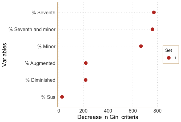
Figure 7: Importance plot for the model with only the first set of variables.

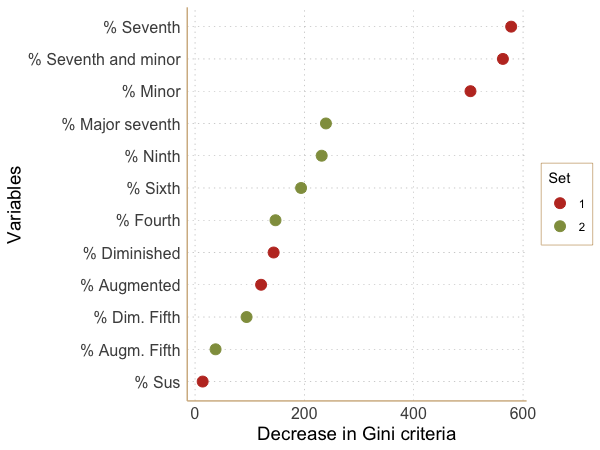
Figure 8: Importance plot for the second model with the first and second sets of variables.

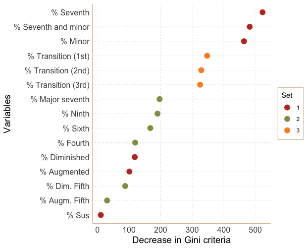
Figure 9: Importance plot for third model with the first, second and third sets of variables.

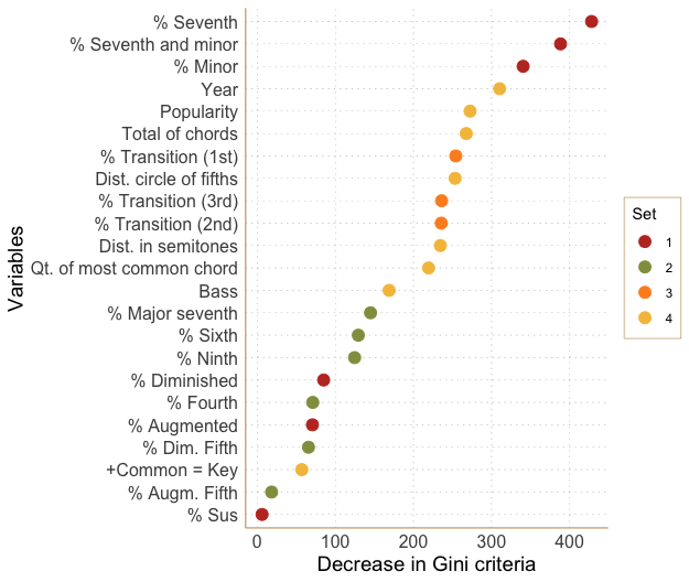
Figure 10: Importance plot for the fourth model with all the considered variables.

At last, we consider the specific importance of the features. An importance plot is used to show the measures of how relevant to the model the features are, by demonstrating the decrease in the Gini criteria attributed to the splits in each variable [32]. Therefore it is easy to perceive the prediction strength of our variables, being that the strongest ones will appear in the top of the plot. Given this and the plot being shown in Figure 7, we notice that the first model has three main variables used in the correct classification: the percentage of chords with the seventh, the percentage of minor chords with the seventh. After the addition of the second set of variables, the same variables have remained on top (Figure 8). By that, we can infer that these three variables have higher discriminant power so far, unlike the second set of variables. The third set of variables, for which the addition is reported on Figure 9, have some strong variables, which are taking place of the old ones when added to the model. This aspect shows that the features of the third set carry a notorious amount of information about the response variables, our music genres. Finally, from the importance plot of the model with all of the variables, shown in Figure 10, we conclude that the most relevant one out of the miscellany set is the year of release of the song, followed by the popularity and the total number of chords in each song. Those features took the place of the ones that were introduced previously, which highlights how informative they are.

In summary, the first set of variables is the most informative one. By using features related to the triads and simple tetrads, the first features set makes it possible for us to separate the nine Brazilain genres, especially for the traditional ones (Table 4). This means that with the basic information about the songs we already obtained good results. The results improved mostly by the addition of external variables, such as the year and popularity of each song, showing how the features from the streaming software Spotify carry relevant information about the boundaries of the evaluated genres. Next, in the importance sequence, we have the transitions and distances variables, strengthening the idea of harmonic characteristics being important to discriminate music genre and also clearing the path about what should be the further steps on the improvement of the analysis.

5 CONCLUSIONS AND DISCUSSION

With our results, we can conclude that is possible to predict music genres of the Brazilian popular music combining features extracted from their harmonic structures and external variables. The overall accuracy of the final model is 62% with a confidence interval of [60%, 64%], being that the better-classified genres are the Brazilian Sertanejo, Samba, MPB (also known as Brazilian Popular Music) and Rock. The most discriminative variables for the model are the percentage of chords with the seventh note, percentage of minor chords with the seventh note, the percentage of minor chords, the year of release of the songs, their popularity, the behavior of the most common chord transitions, the mean distances of the chords having the ’C’ chord in the circle of fifth as a reference and the total number of chords in each song. On this group, prevail the features that can be extracted purely with the symbolic part of the chords. The features obtained with the aid of the Spotify API are also very influent, what makes sense once they came from a very influent music streaming software and its data is reliable [22]. This accentuates how having access to data via the Spotify API is useful and pertinent to research in general.

We emphasize that method for the obtention of the data is implemented in the chorrrds package for R [23]. If data for different artists is required, the package would be the best the option for that task. Moreover, every step of this analysis can be reproduced using the code available at:
https://github.com/brunaw/genre_classification It is very important for the authors that not only this work is entirely reproducible, but can also be easily extended.

Next steps of this work include specially the engineering of the new variables and applying different algorithms to model the data. The modeling section can be improved in two fundamental ways: changing the algorithm itself for another suitable technique and improving the existent model. Options of possible new modeling techniques would be deep learning models [38] and naive Bayes models [39]. References about similar approaches using deep learning can be found in [40] and [41].

As for changing the existing model, alternatives are removing non-informative variables and creating new ones. Using the importance criterion, we have a very good direction about which variables should be reconsidered to be kept in the model. More sophisticated techniques such as Principal Component Analysis [42] could also play an important role in the task of reducing the dimension of columns used in the model. Analogously, reducing the amount of observations is considered a potential next step. The idea here is to find the songs that carry most part of the variance for each genre and thereby can be useful to summarize them, allowing us to use less data to obtain similar results. Regardless of that, finding ways of engineering new variables is a key point of interest. As the main goal of this work is focused on showing how Brazilian music genres can be predicted using interpretable engineered features, assessing more information about the songs via the creation of more features is essential.

References

- [1] Waldenyr Caldas. Iniciação à Música Popular Brasileira, volume 1. 2010.
- [2] Jennifer C. Lena and Richard A. Peterson. Classification as culture: Types and trajectories of music genres. American Sociological Review, 2008.
- [3] Jin Ha Lee and J Stephen Downie. Survey of music information needs, uses, and seeking behaviours: preliminary findings, 2004.
- [4] Automatic chord recognition for music classification and retrieval. In 2008 IEEE International Conference on Multimedia and Expo, ICME 2008 - Proceedings, 2008.
- [5] Débora C. Corrêa and Francisco Ap Rodrigues. A survey on symbolic data-based music genre classification, 2016.
- [6] R.C. Albin. O livro de ouro da MPB: a história de nossa música popular de sua origem até hoje. Livros de ouro. Ediouro, 2003.
- [7] John Ashley Burgoyne, Ichiro Fujinaga, and J. Stephen Downie. Music Information Retrieval. In A New Companion to Digital Humanities. 2015.
- [8] Elias Pampalk, Arthur Flexer, and Gerhard Widmer. Improvements of Audio-Based music similarity and genre classification. In ISMIR, 2005.
- [9] George Tzanetakis and Perry Cook. Musical genre classification of audio signals. IEEE Transactions on Speech and Audio Processing, 2002.
- [10] Hareesh Bahuleyan. Music Genre Classification using Machine Learning Techniques. 2018.
- [11] Nicolas Scaringella, Giorgio Zoia, and Daniel Mlynek. Automatic genre classification of music content. IEEE Signal Processing Magazine, 2006.
- [12] Yair Neuman, Leonid Perlovsky, Yochai Cohen, and Danny Livshits. The personality of music genres. Psychology of Music, 2016.
- [13] Ching-Hua Chuan, Kat Agres, and Dorien Herremans. From Context to Concept: Exploring Semantic Relationships in Music with Word2Vec. nov 2018.
- [14] Carlos Pérez-Sancho, David Rizo, José M. Iesta, Pedro J.Ponce De León, Stefan Kersten, and Rafael Ramirez. Genre classification of music by tonal harmony. Intelligent Data Analysis, 2010.
- [15] The mystery of samba : popular music & national identity in Brazil. 1999.
- [16] Gerard Béhague. Brazilian Musical Values of the 1960s and 1970s: Popular Urban Music from Bossa Nova to Tropicalia. The Journal of Popular Culture, 1980.
- [17] Bryan McCann. Blues and Samba: Another Side of Bossa Nova History. Luso-Brazilian Review, 2007.
- [18] Meinard Müller. Information retrieval for music and motion. 2007.
- [19] Carlos Almada. Harmonia Funcional, volume 1. 2012.
- [20] Robert Rowe. :The Cognition of Basic Musical Structures. Music Perception, 2005.
- [21] Stefano M. Iacus. Automated Data Collection with R - A Practical Guide to Web Scraping and Text Mining. Journal of Statistical Software, 2015.
- [22] Vinicius J. Schettino, Regina Braga, José Maria N. David, and Marco Antônio P. Araújo. In Proceedings of the 11th Brazilian Symposium on Software Components, Architectures, and Reuse - SBCARS ’17.
- [23] Bruna Wundervald. The chorrrds package for extraction of music chords data in r, 2018.
- [24] R Core Team. R: A Language and Environment for Statistical Computing. R Foundation for Statistical Computing, Vienna, Austria, 2018.
- [25] M. Kuhn and K. Johnson. Feature Engineering and Selection: A Practical Approach for Predictive Models. 2018.
- [26] Fatemeh Nargesian, Horst Samulowitz, Udayan Khurana, Elias B Khalil, and Deepak Turaga. Learning feature engineering for classification. In Proceedings of the 26th International Joint Conference on Artificial Intelligence, pages 2529–2535. AAAI Press, 2017.
- [27] D Lewin. A formal theory of generalized tonal functions. Journal of Music Theory, 1982.
- [28] Toward a Formal Theory of Tonal Music. Journal of Music Theory, 1977.
- [29] Brandt Absolu, Tao Li, and Mitsunori Ogihara. Analysis of chord progression data. Studies in Computational Intelligence, 2010.
- [30] J J Faraway. Extending the Linear Model with R: Generalized Linear, Mixed Effects and Nonparametric Regression Models. Chapman & Hall/CRC Texts in Statistical Science. CRC Press, 2016.
- [31] Carl Kingsford and Steven L Salzberg. What are decision trees? Nature Biotechnology, 2008.
- [32] Jerome Hastie, Trevor, Tibshirani, Robert, Friedman. The Elements of Statistical Learning, Second Edition. 2009.
- [33] Leo Breiman. Random forests. Machine Learning, 2001.
- [34] B. Efron. Bootstrap Methods: Another Look at the Jackknife. The Annals of Statistics, 1979.
- [35] Simon Bernard, Laurent Heutte, and Sébastien Adam. A study of strength and correlation in random forests. In Communications in Computer and Information Science, 2010.
- [36] Jacob Cohen. A Coefficient of Agreement for Nominal Scales. Educational and Psychological Measurement, 1960.
- [37] Robert G. D. (Robert George Douglas) Steel and 1908 Torrie, James H. (James Hiram). Principles and procedures of statistics : with special reference to the biological sciences. New York : McGraw-Hill, 1960. Includes bibliographical references.
- [38] Yann Lecun, Yoshua Bengio, and Geoffrey Hinton. Deep learning, 2015.
- [39] Kevin P Murphy. Naive Bayes classifiers. Bernoulli, 2006.
- [40] Hareesh Bahuleyan. Music genre classification using machine learning techniques. CoRR, abs/1804.01149, 2018.
- [41] Sergio Oramas, Oriol Nieto, Francesco Barbieri, and Xavier Serra. Multi-label music genre classification from audio, text, and images using deep features. CoRR, abs/1707.04916, 2017.
- [42] I T Jolliffe. Principal Component Analysis. Second Edition. 2002.