REACTOR NEUTRINOS: TOWARD OSCILLATIONS

Invited Talk at the ”History of the Neutrino” Conference, September 2018, Paris

Abstract

I shall sketch the history of reactor neutrino physics over five decades since the Reines-Cowan proof of neutrino existence in the late 50s, till the advent of the present era of precision reactor neutrino oscillation experiments. There are three chapters of this story: i) Exploration of possibilities of the reactor neutrinos in the 60s and 70s; ii) Looking for oscillations under the streetlamp in the 80s and 90s; iii) Exploring oscillations in detail with known (almost) $\Delta m^{2}_{atm}$ and $\Delta m^{2}_{sol}$.

1 Introduction

Nuclear reactors are powerful sources of low energy electron antineutrinos. The $\bar{\nu}_{e}$ are produced in the $\beta$ decay of the neutron rich fission fragments. Each of the fragments produces on average 3 $\bar{\nu}_{e}$; there are thus $\sim$ 6 $\bar{\nu}_{e}$ per each act of fission. A typical power reactor of 3 GW thermal power undergoes $\sim 10^{20}$ fissions/s and thus produces $\sim 6\times 10^{20}$ $\bar{\nu}_{e}$/s with energies typical for nuclear $\beta$ decay. The $\bar{\nu}_{e}$ spectrum fast decreases with increasing energy, there are only very few $\bar{\nu}_{e}$ left past 8 MeV.

Neutrinos interact with anything else only by weak interactions. It is easy to estimate the order of magnitude of the corresponding cross section. At low energies ($\sim$ MeV) the cross section can depend only on the $\bar{\nu}_{e}$ energy, and must be proportional to $G_{F}^{2}$ ($G_{F}=1.17\times 10^{-11}$ MeV^-2). By dimensional arguments then $\sigma\sim G_{F}^{2}E^{2}(\hbar c)^{2}\sim 10^{-44}$ cm². This is, basically, the argument first made by Bethe and Peierls already in 1934 [1].

Electron antineutrino at nuclear reactors can interact by both charged and neutral weak currents. The following four reactions have been successfully observed:

reaction	label	$\sigma$ (10-44cm2/fission)	threshold (MeV)
$\bar{\nu}_{e}+p\rightarrow e^{+}+n$	ccp	63	1.8
$\bar{\nu}_{e}+d\rightarrow e^{+}+n+n$	ccd	1.1	4.0
$\bar{\nu}_{e}+d\rightarrow\bar{\nu}_{e}+p+n$	ncd	3.1	2.2
$\bar{\nu}_{e}+e^{-}\rightarrow\bar{\nu}_{e}+e^{-}$	el.sc.	0.4	1-6 (range)

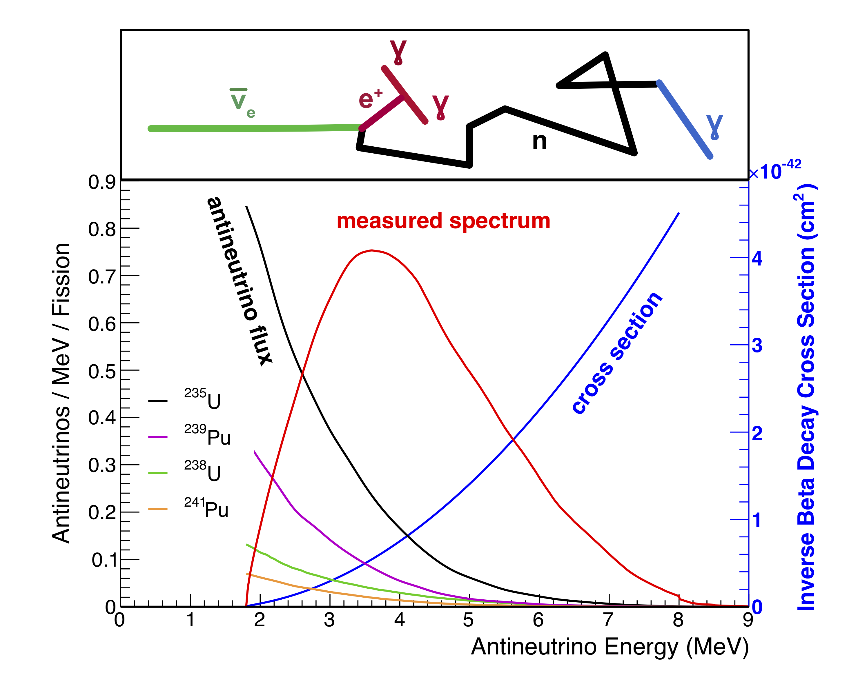
Neutrino capture on protons (ccp), usually called ‘Inverse Beta Decay’ (IBD), has obvious advantages. It has much larger cross section and the neutron recoil energy is low so that the positron carries essentially all available energy. The neutron is eventually captured either on one of the target protons (2.2 MeV capture energy) or is captured on some added admixture with very large neutron capture cross section, such as Gd (8.0 MeV cascade of $\gamma$). The space and time coincidence requirement between the positron detection and neutron capture $\gamma$ rays is a powerful tool for background suppression. The IBD reaction was first used in the Reines-Cowan series of experiments that showed existence of neutrinos as elementary particles [2].

In fig. 1, reproduced from [3], a typical $\bar{\nu}_{e}$ interaction spectrum is shown, the product of decreasing $\bar{\nu}_{e}$ reactor spectrum and increasing interaction cross section. The IBD cross section is simply related (in the zeroth approximation) to the rate of the neutron beta decay $n\rightarrow p+e^{-}+\bar{\nu}_{e}$, namely $\sigma=2\pi^{2}/m_{e}^{5}\times E_{e}p_{e}/f\tau_{n}$, where $E_{e},p_{e}$ are the positron energy and momentum, $f$ is the neutron beta decay phase space integral and $\tau_{n}$ is the neutron lifetime. Corrections to this formula, including the effects of the neutron recoil, weak magnetism, and QED are derived, e.g. in ref. [4].

Figure 1: Reactor $\bar{\nu}_{e}$ flux, inverse-beta-decay cross section, and $\bar{\nu}_{e}$ interaction spectrum. The flux for individual fuel isotopes, weighed by their typical contribution to the total flux in commercial reactors, is also shown. The steps involved in the detection are schematically indicated at the top of the figure. Reproduced from [3].

2 Exploring the possibilities in the 60s and 70s

In the 60s and 70s study of neutrinos was not at the forefront of particle physics. Given the obvious difficulty of observing neutrino induced reactions, it took the dedication and pioneering spirit of Frederic Reines and his collaborators to observe all of the above listed reactions with reactor $\bar{\nu}_{e}$. The ccd and ncd reactions on deuteron targets were observed in [5] and the $\bar{\nu}_{e}$ - electron scattering, with the destructive interference of the charged and neutral currents, and possible electromagnetic interaction if neutrinos have magnetic moments, were observed in [6]. While the measurement of reactions on deuterons was never so far repeated by anybody else, the electron scattering is one of the most sensitive probes of the possible neutrino magnetic moment and is a subject of repeated searches.

These experiments, with detectors very close to the reactor core, demonstrated that the detection of reactor neutrinos is possible with detectors on the surface, essentially unprotected from cosmic rays. They also showed that it is possible to overcome the reactor associated backgrounds.

3 Looking for oscillations under the streetlamp in the 80s and 90s

In late 70s the idea of neutrino oscillations became a hot subject widely discussed in the community (note that the famous Physics Reports review by Bilenky and Pontecorvo appeared in 1978 [7].) As far as the reactor neutrinos are concerned, the only channel open to experimental study is the $\bar{\nu}_{e}$ disappearance; the energy is too low that only positrons can be produced, not $\mu^{+}$ or $\tau^{+}$ leptons. Assuming that the neutrino oscillations can be described as involving just two neutrino flavors, the probability that a $\bar{\nu}_{e}$ of energy $E_{\nu}$ will change into another flavor neutrino $\bar{\nu}_{x}$ is

$$P(\bar{\nu}_{e}\rightarrow\bar{\nu}_{x})=\sin^{2}2\theta\sin^{2}\frac{1.27\Delta m^{2}{\rm(eV)}^{2}L{\rm(m)}}{E_{\nu}{\rm(MeV)}}\leavevmode\nobreak\ .$$ (1)

The corresponding phenomenological parameters, the mixing angle $\theta$ and the mass squared difference $\Delta m^{2}$ were totally unknown at that time. Hence, experiments were set up ‘under the streetlamp’, that it where it was relatively easier to perform them.

Reactor experiments with $\sim$ MeV neutrinos were reasonably realistic at that time, with few hundred kg of the hydrogen containing detectors at $L<$ 100 m from the reactor core, that would be sensitive to the oscillations with $\Delta m^{2}$ near 1 eV². Large number (more that 20) of such experiments were performed, at that time constraining the $\Delta m^{2}$ in the indicate range and a relatively large mixing angles.

These were all ‘one detector’ experiments, in which the signal at $L$ was compared to expected signal at $L=0$, i.e. to the spectrum of the $\bar{\nu}_{e}$ emitted by the reactor. The knowledge of that spectrum and its uncertainties was, therefore, an essestial ingredient.

I will describe now two of the historically first reactor neutrino oscillation searches.

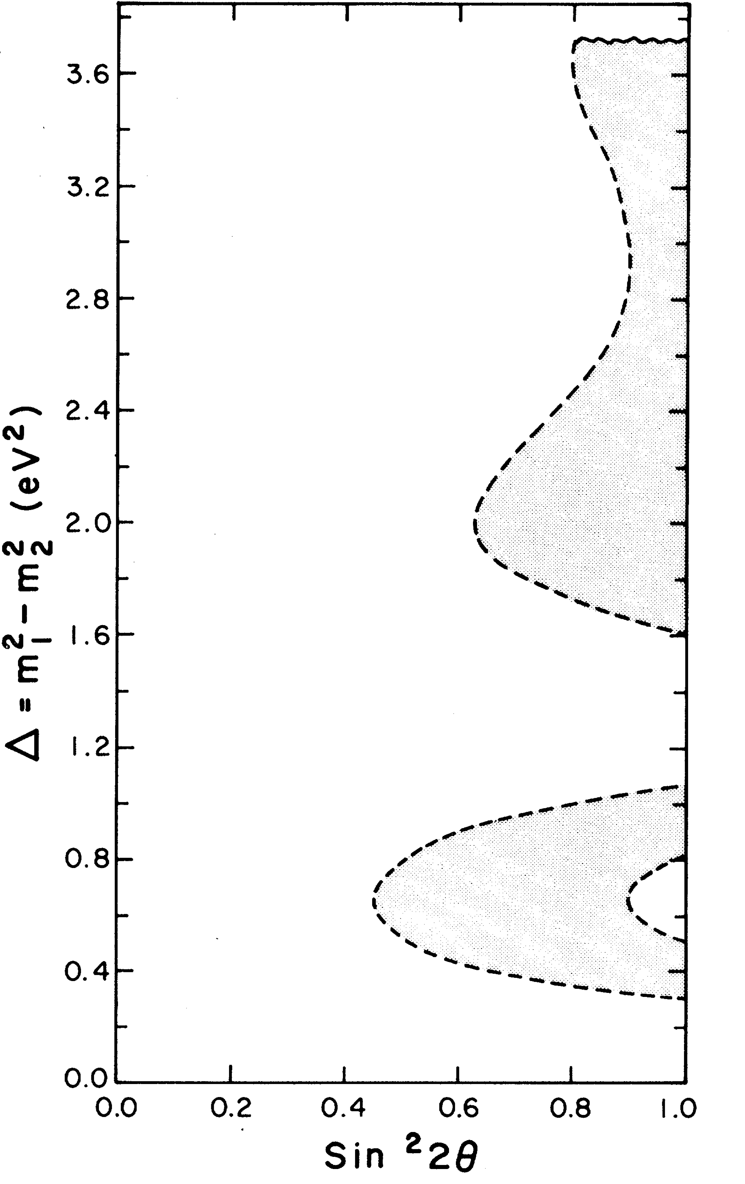
In Ref. [8] the rate of the charged and neutral current deuteron experiments, $\bar{\nu}_{e}+d\rightarrow n+n+e^{+}$ and $\bar{\nu}_{e}+d\rightarrow n+\bar{\nu_{e}}$ were compared. The corresponding thresholds and cross sections are listed in Table I. The 268 kg D₂O detector was placed 11.2 m from the 2000 MW power reactor. Only the neutrons were detected; two neutron events represented the charged current and one neutron events represented the neutral current. Using the calculated reactor neutrino spectrum [9], newly evaluated at that time, the rate of the charged current events was smaller than expectation, 0.44$\pm$0.19, while the rates of the neutral and ccp reactions agreed within errors. This was interpreted as ‘Evidence for Neutrino Instability’. The corresponding allowed region in the $\Delta m^{2}$ and $\sin^{2}2\theta$ is shown in Fig. 2, reproduced from [8].

Figure 2: Grey areas, enclosed in the dashed lines, are the allowed regions of the parameter space. Reproduced from [8].

The paper created a considerable excitement at that time. However, there were also doubts. Why was not disappearance noted in the reaction on protons, which were detected actually at two distances, 6 and 11.2 m ? Also, given the difference in the thresholds of the charged and neutral current reactions, there was an obvious strong dependence on the correct reactor spectrum that changes rapidly between 2 and 4 MeV. The claim was eventually withdrawn [10]; the neutron detection efficiency used was revised. Note, incidentally, that this was not a genuine planned oscillation experiment. The apparatus and some of the data came from Ref. [5].

The ILL experiment [11] was the first experiment built specifically to test the oscillation scenario. It used the 57 MW research reactor at the Institute Laue Langevin in Grenoble, France that uses 93% ²³⁵U enriched fuel. The detector, contained 377 l of liquid scintillator in 5 walls of target cells with 4 sets of ³He wire chambers that detected neutrons in between them. The detector was placed 8.76 m from the compact reactor core.

The detected positron spectrum, together with expectations for no oscillations, is shown in Fig. 3. It is reproduced from ref. [11].

Figure 3: The positron kinetic energy spectrum. The solid line is based on the $\bar{\nu}_{e}$ spectrum, derived from the experimental electron spectrum described later in the text. The D et al. spectrum is the prediction of ref. [9]. The AG spectrum is based on an older evaluation that obviously predicted too many $\bar{\nu}_{e}$ above the threshold. Reproduced from [11].

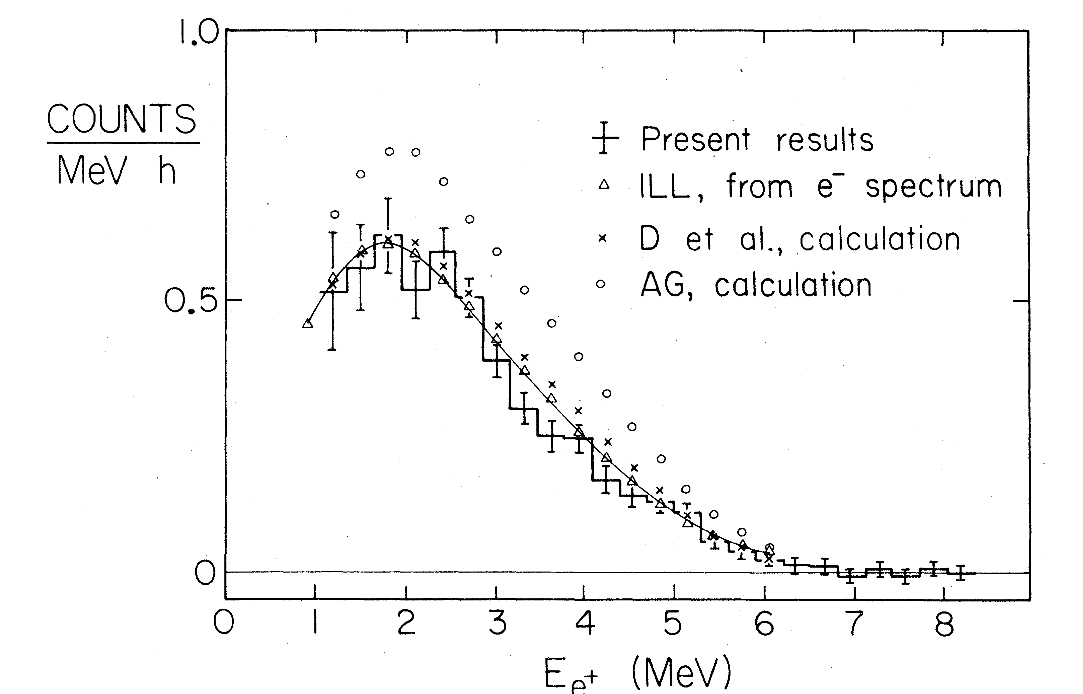
Obviously, no indication of neutrino oscillations was detected. The ratio of the experimental to expected integral positron yield for $E_{e^{+}}>1$ MeV was found to be
$\int Y_{exp}(E_{e^{+}})dE_{e+}/\int Y_{noosc.}(E_{e^{+}})dE_{e+}$ = 0.955$\pm$ 0.035(stat) $\pm$ 0.11(syst).

However, interestingly that is not the end of the story. In 1995, 15 years later, it was announced [12] that the operating power of the high-flux reactor of Institute Laue Langevin (ILL), Grenoble, had been incorrectly reported since its earliest days of operation. One impact of this is that the ILL reactor was operated at the time of the experiment at 1.095 times it’s rated full power ( 57 MW thermal). Therefore, the ILL experiment had to be reanalysed; it showed now a depletion of 17% in the neutrino flux. (Neutron lifetime and few other things were changed together with the reactor power.) Thus the ratio of experimental to expected integral positron yield is now only 0.832$\pm$ 3.5 %(stat) $\pm$ 8.87 %(syst), seemingly indicating $\bar{\nu_{e}}$ disappearance.

But this is unlikely so. A number of analogous experiments, described briefly later, does not show such a substantial depletion. And, in particular, a very similar experiment OSIRIS, [13] on the reactor with a substantial ²³⁵U enrichment (19.75%), like at ILL, with the detector at 7.21 m from the reactor core, gave $R_{obs}/R_{pred}$ = 1.014 $\pm$ 0.108. The ILL result remains unexplained.

Since this conference is about history, it is worthwhile to mention also aspects that are not strictly speaking related to physics, but are nevertheless important to the pursuit of physics results. The issue is the role of the personal contacts in suggesting, planing, funding, and performing experiments. Having good personal contacts considerably helps to some, and not having them is a disadvantage to others. I will illustrate the issue using the ILL experiment as an example. At that time in my home institution, Caltech, there was a very active group of theorists working with Murray Gell-Mann. Among them, in particular, Peter Minkowski and Harald Fritzsch were very interested in neutrino oscillations and strongly encouraged my colleague Felix Boehm to think about possible experimental search. That lead to the idea of a reactor experiment. But where can one find a suitable reactor with potentially supportive administration? That lead again to the ILL reactor where Rudolf Mössbauer, then professor in Munich, Germany, was a current Institute director. He was a former member of Caltech faculty, and was not only enthusiasticaly interested, but became, with his students and collaborators an active part of the team of Caltech, Munich and Grenoble physicists who built and run the reactor neutrino oscillation experiment [11]. This chain of friendships was essential for the success of the experiment.

3.1 Reactor spectrum

Clearly, the knowledge of the reactor neutrino spectrum is crucial. So, how it could be determined? And how it was determined in the past?

There are two ways, each with its strengths and weaknesses, which were developed during that time pariod:

1) Add the beta decay spectra of all fission fragments. That obviously requires the knowledge of the contribution of each fuel isotope to the reactor power, of the fission yields (how often is a given isotope produced in fission), half-lives, branching ratios, and endpoints of all beta branches, and spectrum shape of each of them. And, naturally also, error bars of all of that.

Thus, disregarding for clarity the error bars, the neutrino spectrum can be expressed as

$$S(E_{\bar{\nu}})=\frac{W_{therm}}{\Sigma_{i}(f_{i}/F)e_{i}}\Sigma_{i}\frac{f_{i}}{F}\left(\frac{dN_{i}}{dE_{\bar{\nu}}}\right)\leavevmode\nobreak\ ,$$ (2)

where $W_{therm}$ is the thermal power of the reactor, $f_{i}$ is the number of fissions of the fuel isotope $i$, $F$ is the total number of fissions, $e_{i}$ is the energy per fission, and $dN_{i}/dE_{\bar{\nu}}$ is the spectrum of the fuel isotope $i$. In turn

$$\frac{dN_{i}}{dE_{\bar{\nu}}}=\Sigma_{n}Y_{n}(Z,A,t)\Sigma_{j}b_{n,j}P_{\bar{\nu}}(E_{\bar{\nu}}E_{0}^{j},Z)\leavevmode\nobreak\ ,$$ (3)

where $Y_{n}(Z,A,t)$ is the cumulative yield of the isotope $Z,A$ at time $t$, $b_{n,j}$ is the branching ratio of the $\beta$ branch $j$ and $P_{\bar{\nu}}(E_{\bar{\nu}}E_{0}^{j},Z)$ is the normalized spectrum shape of the branch $j$ with the endpoint $E_{0}^{j}$.

This is seemingly quite straightforward. The thermal power and fission fractions $f_{i}/F$ are typically supplied by the reactor operators and the energy per fission, $e_{i}$, is known with only small uncertainty. There are libraries of fission yields, but some, in particular for isotopes with short half-lives and hence large endpoint energies, have large uncertainties. Some $\beta$ branching ratios and endpoint energies are also poorly known, some are even unknown. And the spectrum shapes are well defined for the allowed beta decays (there are, however, substantial uncertainties in the next order corrections for the nuclear finite size and weak magnetism that account for a few % each), but about 25% of the decays are first forbidden with a more substantial uncertainty in their spectrum. So, the total uncertainty is rather difficult to estimate.

Figure 4: Calculated electron spectra of the ²³⁵U thermal neutron fission. The thin gray lines are from individual $\beta$ decays. The thick (color) lines highlight the 20 most important contributions to energies above 5.5 MeV. The squares are the sum of all decays and the thick blue line is the measures electron spectrum. Reproduced from [14].

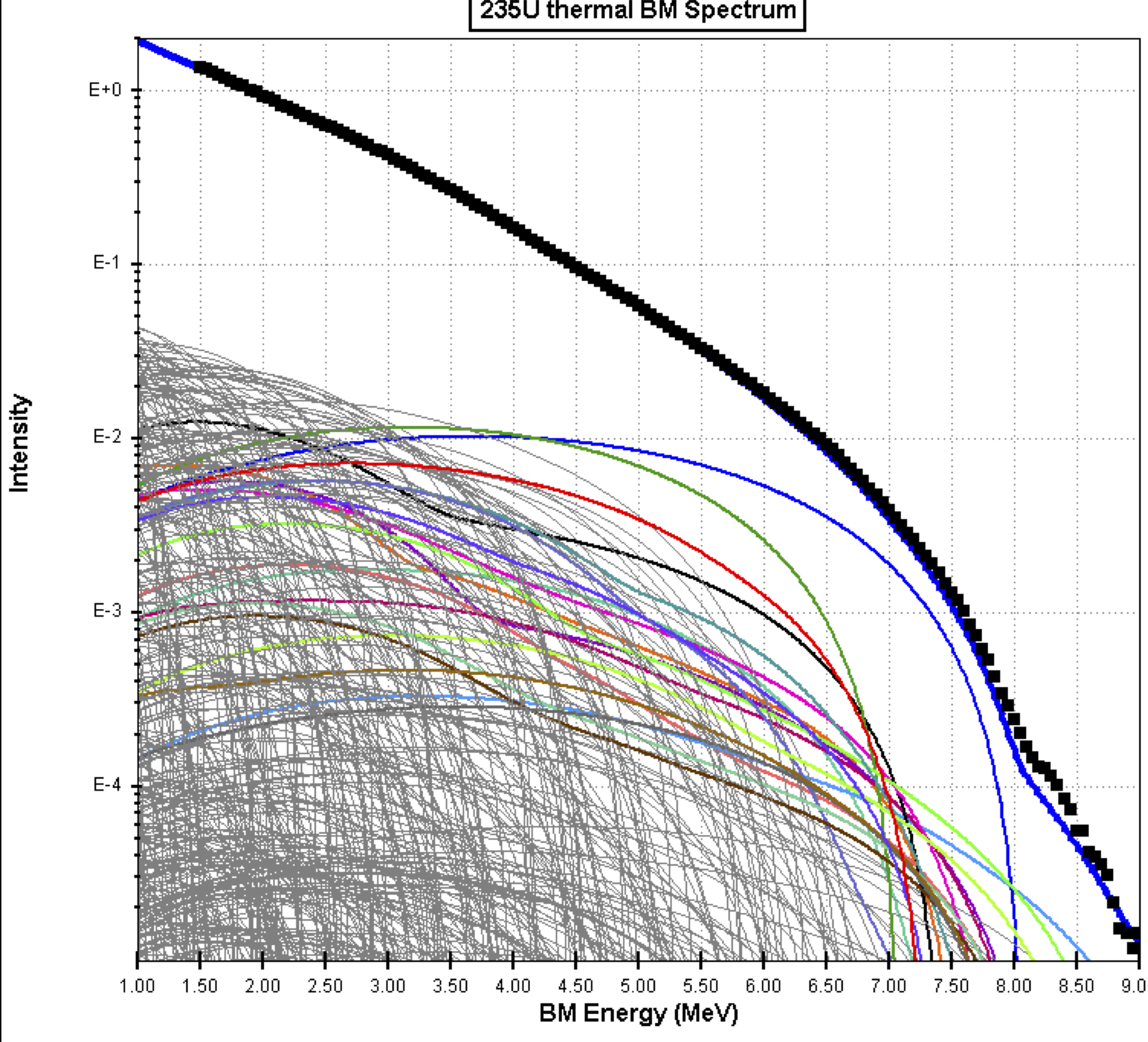
How it is done is illustrated in Fig. 4 reproduced from [14]. There are about 800 individual fission fragments, with several thousand $\beta$ decay branches displayed. As indicated, at higher energies, above $\sim$5 MeV, the number of significant fragments is greatly reduced and the relative contribution of each of them correspondingly enhanced.

This method was used repeatedly [9, 15, 16, 17, 18], by adding newer data and using different ways for treatment the unknown $\beta$ transitions. More recently, in ref. [19], more consistent treatment of corrections to the allowed $\beta$ decay shape, more careful treatment of the fission fragments that do not achieve equilibrium, use of the recently revised neutron life-time as well as normalization to the electron spectrum explained next, resulted in the upward revision of the total $\bar{\nu}_{e}$ flux by $\sim$ 6%, without a substantial change in its shape.

2) The second method uses the experimentally determined electron spectrum associated with fission of each of the reactor fuels. The electron spectrum is then converted into the $\bar{\nu}_{e}$ spectrum using the fact that in each $\beta$ decay branch the electron and the $\bar{\nu}_{e}$ share the available energy $E_{0}^{j}$. The electron spectra associated with the thermal neutron fission of ²³⁵U, ²³⁹Pu and ²⁴¹Pu were determined in a series of experiments [20, 21, 22] at the ILL, Grenoble. ²³⁸U, that contributes $\sim$ 10% to the power of a typical commercial reactor, fissions only with fast neutrons. Its electron spectrum was determined at the reactor in Munich, [23] only recently and with substantially larger uncertainties. The conversion from electrons to $\bar{\nu}_{e}$ is relatively straightforward, see e.g. [24], and does not introduce additional bothersome uncertainty. However, since the fission fragments correspond to a large range of nuclear charges $Z$, and the $\beta$ spectrum shape depends on $Z$ substantially, it is necessary to use the fission and $\beta$ decay libraries in order to evaluate the average $\langle Z\rangle$ as a function of the endpoint energy of the fragments. This information is then used in the conversion procedure.

The $\bar{\nu}_{e}$ spectrum based on the conversion of the experimental ILL electron spectra were a standard used for the analysis of reactor oscillation experiments until $\sim$ 2011. At that time, the results of [19], mentioned earlier, and a new conversion of the ILL spectra in ref. [25] appeared. Both of them [19, 25] rely on the measure ILL electron spectra, thus naturally, they give essentially identical total rate and only slightly different slope of the spectrum. This is used as a standard now. It is remarkable, and a bit unusual, that fundamental input information is based on essentially unique, and so far not repeated experiment. Current reactor experiments, however, avoid most of the related uncertainty by using two sets of detector, one (so-called monitor) closer to the reactor complex, and another one at $L$, further away.

3.2 Reactor anomaly

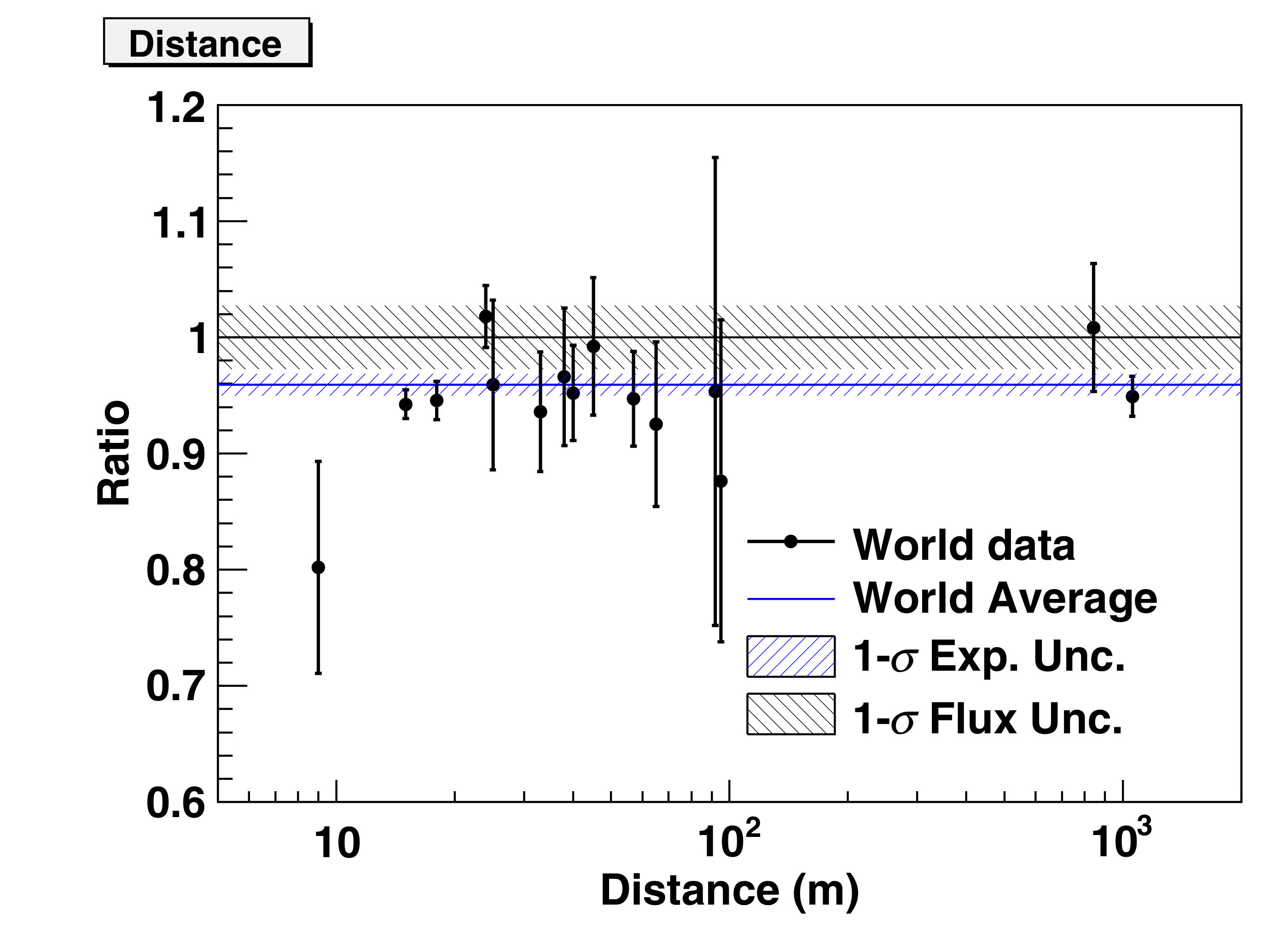
As mentioned earlier, during the 80th and 90th a large number of reactor experiments was performed at distances $L<$ 100 m (for the complete list and corresponding references see, e.g. [27]). All of these measurements are consistent with each other. Resulting total flux is determined to about 1% experimental accuracy. The situation is depicted in Fig. 5, reproduced from [27] which contains also results of some newer experiments at $L\sim$ 1 km.

However, the experimentally determined total flux is $\sim$ 6% less than the prediction based on [19, 25] that has an estimated uncertainty of 2.7%. This discrepancy became known as the “reactor anomaly”. It can be interpreted as a sign of ‘new physics beyond the Standard Model’ [26]. However, it could also, alternatively, mean that the predicted reactor flux is more uncertain that the estimates in [19, 25] suggest, primarily due to the difficulty in accounting for the shape of the first forbidden $\beta$ decays. There is a lively discussion in the physics community about this issue and a large number of experiments, some already running at the present time, is designed to test the beyond the Standard Model hypothesis (see also the contribution of T. Laserre in these proceedings).

Figure 5: Reactor $\bar{\nu}_{e}$ capture rate vs. distance $L$ normalized to the theoretical flux of ref. [19]. The 2.7% reactor flux uncertainty is shown as a band around unity. The (blue) horizontal bar represents the world average and its $1\sigma$ errors. Data at the same $L$ are averaged for clarity. Reproduced from [27].

3.3 The “bump”

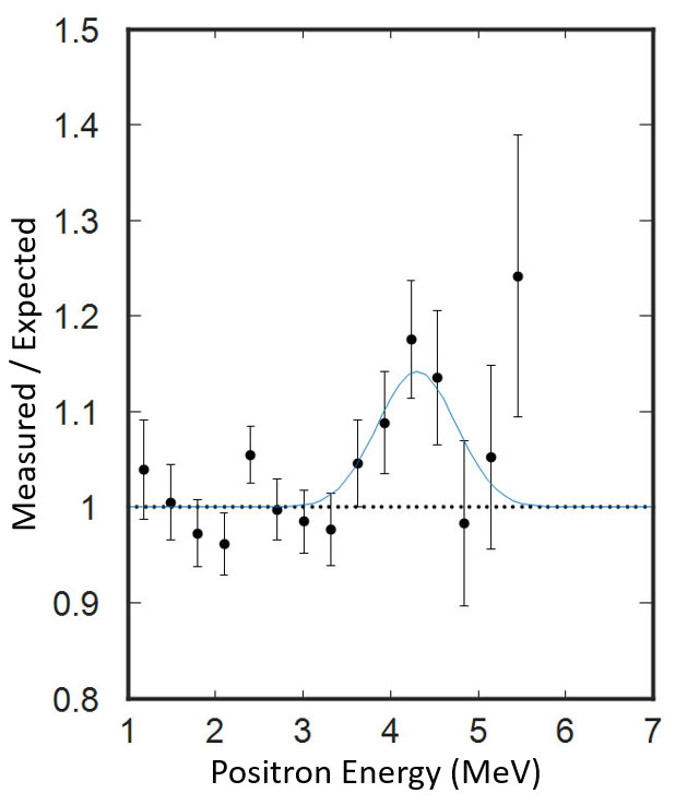
Another unexpected feature in the reactor spectra has been observed in recent reactor experiments (see the discussion in [28] and the list of original references). The shoulder, centered at $\sim$ 5 MeV of the prompt energy, and looking like a broad peak when plotted as the ratio of the observed vs. expected spectrum, became known as the “5 MeV bump”. It does not affect noticeably the corresponding fit to oscillation parameters, but casts some additional doubts on the reliability of the calculated reactor $\bar{\nu}_{e}$ flux. All experiments that observe the bump so far employ large volumes of Gd - loaded liquid scintillator, where the positron energy is recorded together with the two 511 - keV annihilation gamma rays. Is it possible that the ‘bump’ has something to do with this? Such possibility might explain why an earlier experiment [29] with a segmented detector, where only the positron kinetic energy is observed, and a different neutron capture detection process is used, did not observe such spectrum distortion.

However, the reanalysis of the Gösgen experiment [30], another experiment with a segmented detector, shows that the ‘bump’ was in fact present there, as shown in Fig. 6, but unfortunately overlooked at that time. Moreover, the peak in the ratio plot is now near 4.2 MeV, precisely where it should be if it is indeed caused by the IBD reaction. Thus, all that points out that indeed the calculated spectra, related all to the ILL experiments [20, 21, 22], somehow miss this feature.

Figure 6: Ratio of the combined measured energy spectrum (black dots) to the predicted spectrum. The gaussian fit to the data is indicated. Reproduced from [31].

4 Exploring the neutrino oscillations with (almost) known $\Delta m^{2}$

In the late 90th the era of blind exploration came to an end. The phenomenon of neutrino oscillations was, at least tentatively, established. Study of atmospheric neutrinos led to the assignment of $\Delta m^{2}_{atm}\sim(2-4)\times 10^{-3}$ eV² while the study of solar neutrinos had, still, several possible solutions, but increasingly the Large Mixing Angle (LMA) with $\Delta m^{2}_{sol}\sim 10^{-4}$ eV² became the preferred one. Both of these disappearance channels were characterized by relatively large mixing angles thus opening the way for the reactor experiments exploring them.

For the reactor neutrino physics it suggested two areas:
a) Perform experiments at $\sim$ 1 km corresponding to the $\Delta m^{2}_{atm}$ and try to determine or constrain the mixing angle $\theta_{13}$. Note that atmospheric neutrinos, with nearly maximal $\nu_{\mu}\rightarrow\nu_{\tau}$ oscillation probability are insensitive to $\theta_{13}$. This program was realized by the Chooz and Palo Verde experiments in the late 90th and early 2000. This effort and its successful continuation is discussed in detail by T. Laserre in these proceedings.
b) Perform an experiment at $\sim$ 100 km corresponding to the $\Delta m^{2}_{sol}$ and try to demonstrate the validity of the oscillation interpretation of the solar neutrino observations also for $\bar{\nu}_{e}$ at a terrestrial experiment and without the matter effects. This program was realized by the KamLAND experiment.

Going from $\sim$ 100 m from the reactor core to $\sim$ 100 km represents an obvious challenge since the $\bar{\nu}_{e}$ flux is reduced by the factor of million. The detector must be much larger and much better shielded against cosmic rays. And all other backgrounds must be substantially reduced as well. And, in addition, as many reactors as possible should contribute in unison.

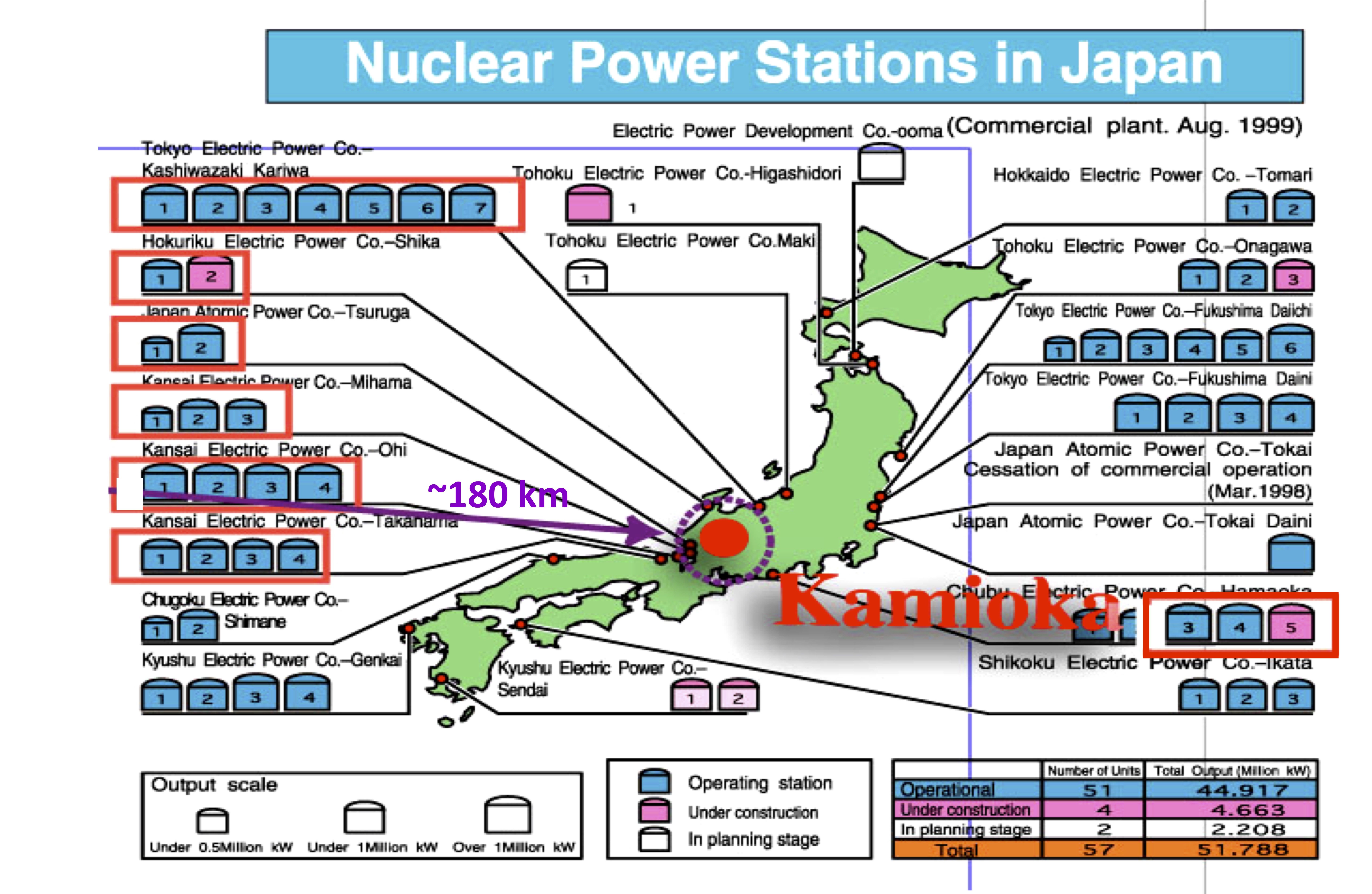
The unique combination of all of that was realized in the KamLAND experiment. At that time there were $\sim$ 40 working power reactors in Japan. And, by a happy coincidence, many of them were situated approximately at a circle with radius $\sim$ 180 km centered around Kamioka, as illustrated in Fig. 7. And in Kamioka an underground site became available when the original Kamiokande experiment was decommissioned.

Figure 7: Nuclear power reactors in Japan. The ‘magic circle’ of reactors around Kamioka is indicated.

KamLAND detector/target contains 1 kt of ultrapure liquid scintillator; both the $e^{+}$ and the 2.2 MeV photons from the neutron capture on hydrogen are detected in the space and time coincidence. Observing the IBD events was possible thanks to the unprecendented radiopurity of the scintillator liquid. The amount of ²³⁸U and ²³²Th was reduced to $(3.8\pm 0.5)\times 10^{-18}$ g/g and $(5.2\pm 0.8)\times 10^{-17}$ g/g, respectively. The observed IBD rate was $\sim$ 0.3/ton$\cdot$year, well above the really low background.

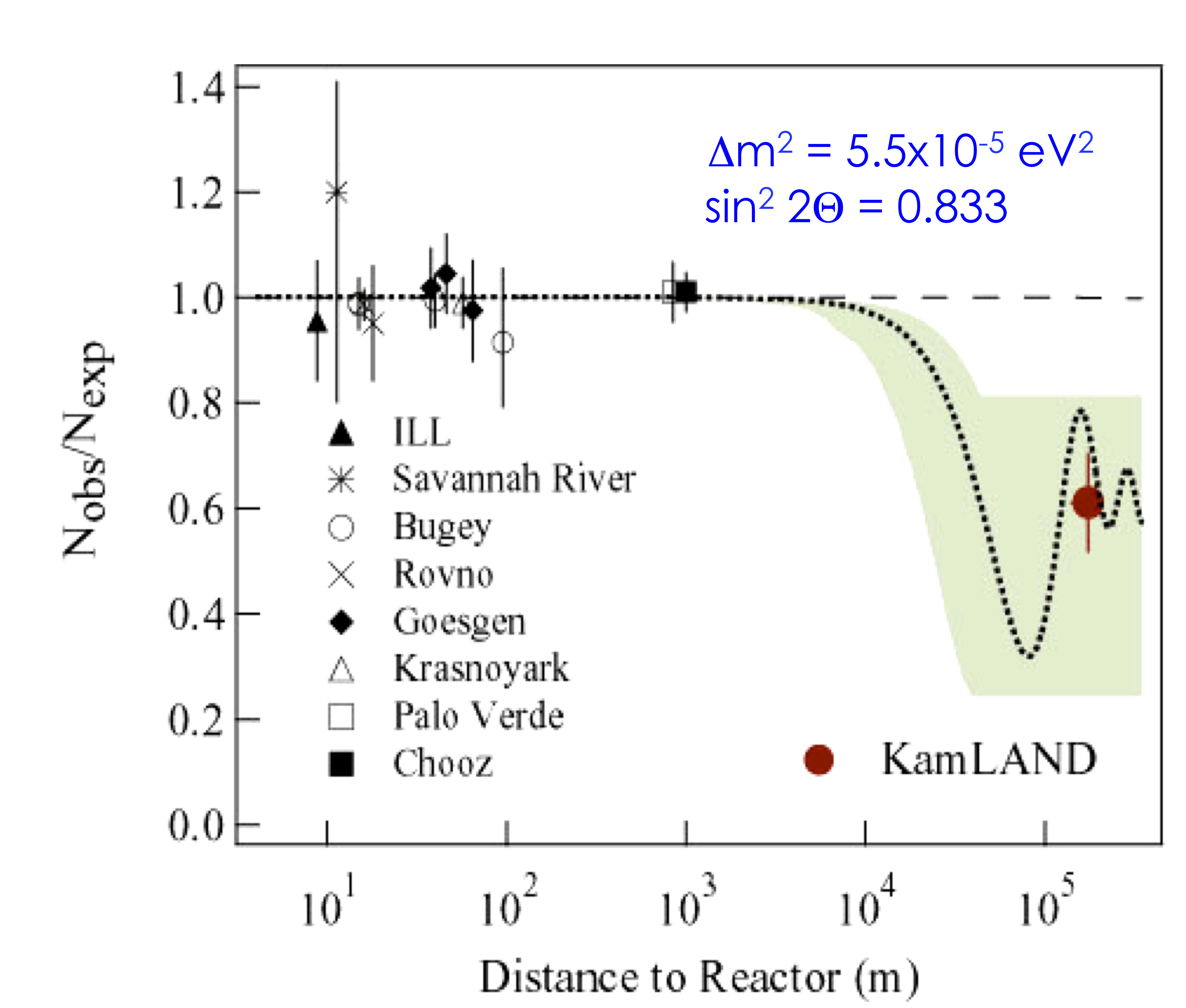
Already the first KamLAND result [32], using the exposure of 162 ton$\cdot$year, shows clear $\bar{\nu}_{e}$ disappearance. The ratio of the observed IBD events to the expectations is $0.611\pm 0.085{\rm\leavevmode\nobreak\ (stat)}\pm 0.041$ (syst) for $\bar{\nu}_{e}$ energies above 3.4 MeV. In Fig. 8, reproduced from [32], these results are plotted together with the results of the previous, shorter baseline, reactor experiments. Not only is the $\bar{\nu}_{e}$ disappearance obvious, but it also demonstrates that this result is in clear agreement with the solar neutrino observations, confirming the LMA solutions.

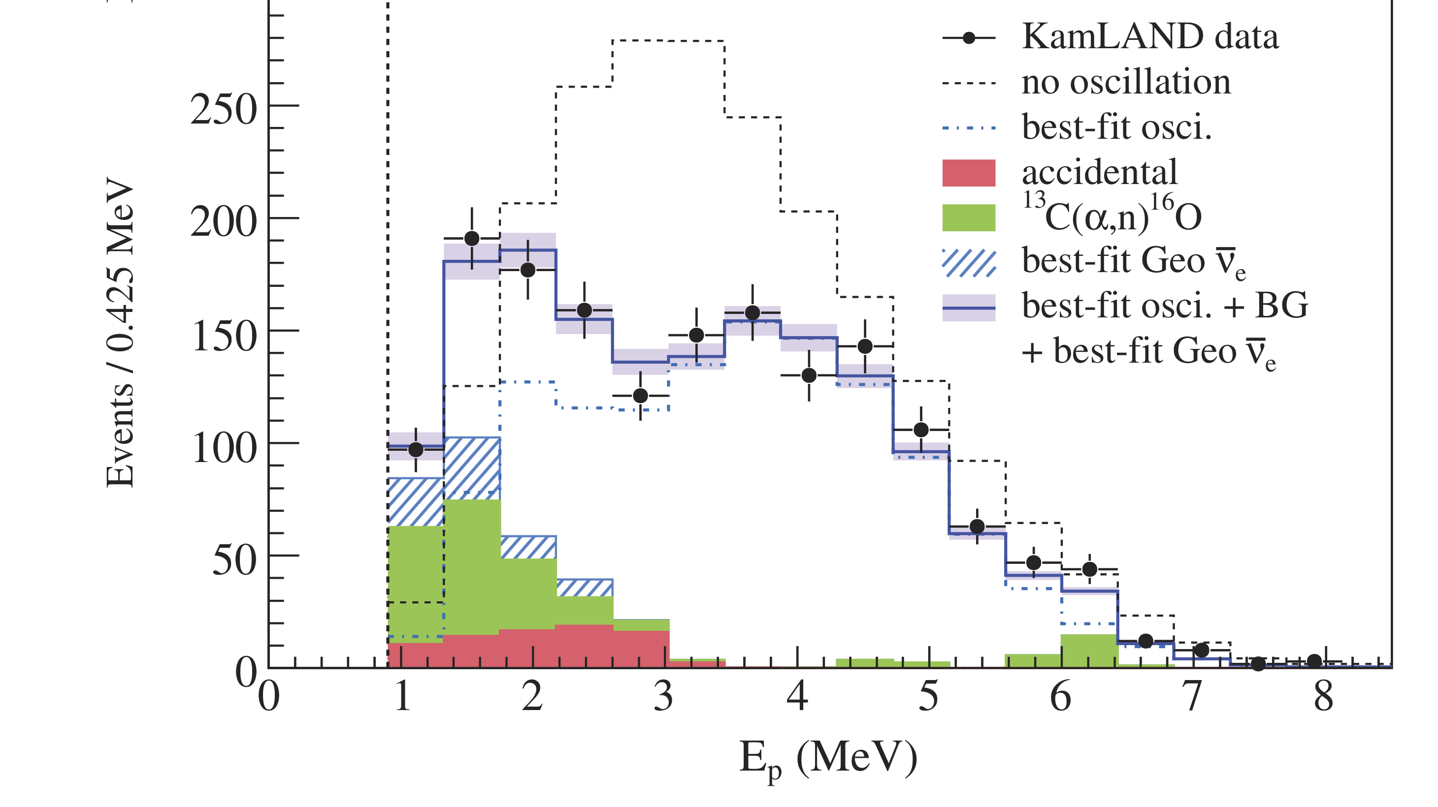
Further exposure with significantly more data (2881 ton$\cdot$year) made it possible to determine the oscillation parameters with substantially more precision [33]. An undistorted (i.e. no oscillation) reactor $\bar{\nu}_{e}$ spectrum is now rejected at $>5\sigma$. The best fit to the spectrum gives $\Delta m_{21}^{2}=7.68^{+0.15}_{-0.14}{\rm(stat)}\pm 0.15{\rm(syst)}\times 10^{-5}$ eV², i.e. determination with $\sim$ 2.5% accuracy. Other local minima of $\Delta m_{21}^{2}$ are disfavored at $>4\sigma$, that is the LMA solution is firmly established. The experimental reactor $\bar{\nu}_{e}$ spectrum is compared to the no oscillation expectation in Fig. 9 reproduced from [33]. The figure also shows various background components; the background is well understood.

Figure 8: The ratio of measured to expected $\bar{\nu}_{e}$ flux from indicated reactor experiments. The solid circle is the KamLAND result plotted at a flux-weighted average distance of $\sim$180 km. The shaded region indicates the range of flux predictions corresponding to the 95% C.L. LMA region from a global analysis of the solar neutrino data. The dotted curve is representative of a best-fit LMA prediction. Reproduced from [32].

From the historical perspective another first for KamLAND should be mentioned, even though it is unrelated to nuclear reactors. For the first time the so called geoneutrinos, $\bar{\nu}_{e}$ produced by the decay of ²³⁸U and ²³²Th within Earth, were detected [34]. Earth composition models suggest that the radiogenic power from these isotopes accounts for approximately half of the total measured heat dissipation rate from the Earth. Although KamLAND data have limited statistical power, they nevertheless provide, by direct means, an upper limit (60TW) for the radiogenic power of U and Th in the Earth, a quantity that is currently poorly constrained.

Figure 9: Prompt $\bar{\nu}_{e}$ energy spectrum. Various background components are indicated. The blue histogram indicates the event rate systematic uncertainty. Reproduced from [33].

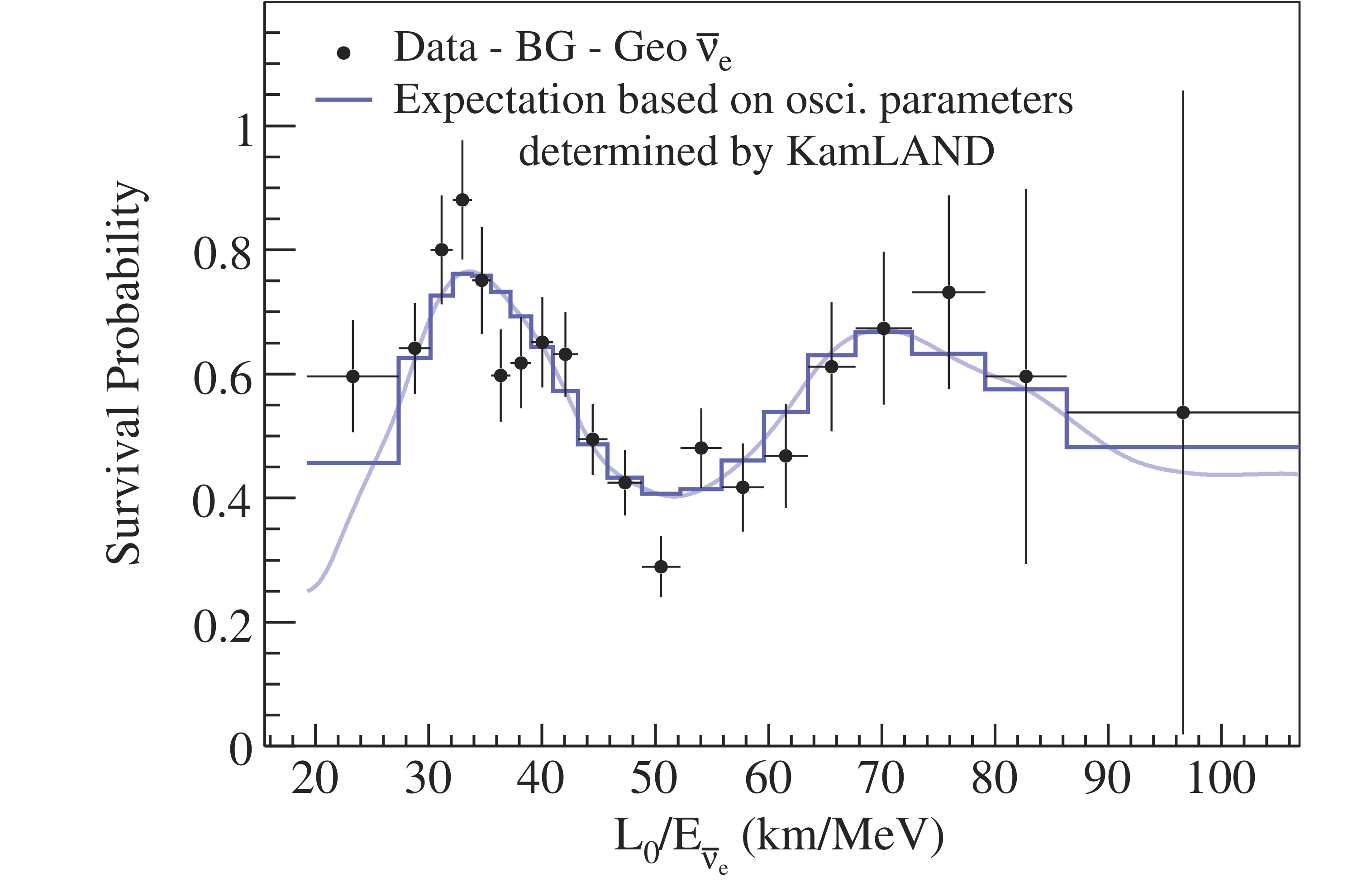
The ultimate test of the neutrino oscillation phenomenon is an observation of the periodic changes of the detection probability of a given neutrino flavor, as prescribed by the eq. (1). Just an observation of the disappearance of the initial neutrino flavor, or appearance of another one, is a necessary condition of the oscillation scenario, but not necessarily sufficient one. As shown in Fig.10, reproduced from [33], KamLAND results show that the disappearance probability of the reactor $\bar{\nu}_{e}$ indeed changes periodically as the function of $L/E_{\nu}$. Two full periods are clearly visible. This was the first time this was accomplished.

There are, naturally, some caveats. The background needs to be subtracted. And the rate has to be normalized to the no oscillation expectation. And in KamLAND the distance $L$ is not well defined, since the signal comes from many reactors. However, 86% of all $\bar{\nu}_{e}$ events come from the distance 175$\pm$ 35 km. In fact, the histogram and curve show the expectation accounting for the distances to the individual reactors. Thus, the periodic behavior is well supported.

Figure 10: Ratio of the background and geoneutrino- subtracted $\bar{\nu}_{e}$ spectrum to the expectation for no-oscillation as a function of $L_{0}/E$. $L_{0}$ is the effective baseline taken as a flux- weighted average ($L_{0}$ = 180 km). Reproduced from [33].

5 Conclusions

In this brief contribution I tried to highlight the development of the study of reactor neutrinos over several decades. Many things happened from the early days exploring the exotic, incredibly weakly interacting particles, to the present tool of precision experiments. And the story is far from over. Several large long baseline experiments are being prepared for data taking, with the goal of determining the neutrino mass hierarchy, a really challenging task. And the ‘reactor anomaly’ is a hot subject these days, with many short baseline reactor experiments competing for the goal of either proving that additional sterile neutrinos indeed exist or that, at least in the context of reactor neutrinos, this is a false alarm. So stay tuned.

References

- [1] H. Bethe and R. Peierls, Nature 133, 532 (1934).
- [2] F. Reines and C. L. Cowan Jr., Phys. Rev. 92, 830 (1953); C.L. Cowan Jr. et al. Science 124, (3212), 103, (1956); F. Reines et al. Phys. Rev. 117, 159 (1960).
- [3] P. Vogel, L.J. Wen, C. Zhang, Nature Communications, 6, 6935 (2015).
- [4] P. Vogel and J. F. Beacom, Phys. Rev. D60, 053003 (1999).
- [5] E. Pasierb et al. , Phys. Rev. Lett. 43, 96 (1979).
- [6] F. Reines et al., Phys. Rev. Lett. 37, 315 (1976).
- [7] S. M. Bilenky and B. Pontecorvo, Phys, Rep. 41, 225 (1978).
- [8] F. Reines, H.W. Sobel and E. Pasierb, Phys. Rev. Lett. 45, 1307 (1980).
- [9] B. R. Davis, P. Vogel, F. M. Mann and R. E. Schenter, Phys. Rev. C 19, 2259 (1979).
- [10] F. Reines, Nucl. Phys. A396, 469c (1983).
- [11] H. Kwon et al. Phys. Rev. D 24, 1097 (1981).
- [12] A. Houmadda et al. AppL Radiat. Isot. 46, 449 (1995).
- [13] G. Boireau et al. Phys.Rev.D93, 112006 (2016).
- [14] A. A. Sonzogni, T.D.Johnson and E.A. McCutchan, Phys. Rev.C91, 011301 (2015).
- [15] P. Vogel, G. K. Schenter, F. M. Mann, and R. E. Schenter, Phys. Rev. C24 1543 (1981).
- [16] H. V. Klapdor and J. Metzinger, Phys. Rev. Lett. 48, 527 (1982); Phys. Lett. B112, 22 (1982).
- [17] O. Tengblad et al., Nucl. Phys. bf A503, 136 (1989).
- [18] V. I. Kopeikin, L. A. Mikaelyan and V. V. Sinev, Phys. At. Nucl. 60, 172 (1997).
- [19] T. A. Mueller et al. Phys. Rev. C83, 054615 (2011).
- [20] F. v. Feilitzsch, A. A. Hahn, K. Schreckenbach, Phys. Lett. B118, 365 (1982).
- [21] K. Schreckenbach, G. Colvin, W. Gelletly, and F. v. Feilitizsch, Phys. Lett. B160, 325 (1985).
- [22] A. A. Hahn et al. Phys. Lett. B218, 365 (1989).
- [23] N. Haag et al. Phys. Rev. Lett 112,122501 (2014).
- [24] P. Vogel, Phys. Rev. C76, 025504 (2007).
- [25] P. Huber, Phys. Rev. C84, 024617 (2011); erratum, ibid 85, 029901 (2012).
- [26] G. Mention et al., Phys. Rev. D83, 073006 (2011).
- [27] C. Zhang, X. Qian and P. Vogel, Phys. Rev. D87, 073018 (2013).
- [28] A. Hayes and P. Vogel, Annu. Rev. Nucl. Part. Sci.66,219 (2016).
- [29] B. Achbar et al. Nucl. Phys. B374, 243 (1996).
- [30] G. Zacek et al., Phys. Rev. D 34, 2621 (1986).
- [31] V. Zacek et al., Phys. Rev. C (to be published); arXiv:1807.01810.
- [32] K. Eguchi et al., Phys. Rev. Lett. 90, 021802 (2003).
- [33] S. Abe et al., Phys. Rev. Lett. 100, 0221803 (2008).
- [34] T. Araki et al., Nature 436, 499 (2005).