Generalized Regular $\mathbf{k}$-point Grid Generation On The Fly

Abstract

In the DFT community, it is common practice to use regular $\mathbf{k}$-point grids (Monkhorst-Pack, MP) for Brillioun zone integration. Recently Wisesa et. al.Wisesa et al. (2016) and Morgan et. al.Morgan et al. (2018) demonstrated that generalized regular (GR) grids offer advantages over traditional MP grids. GR grids have not been widely adopted because one must search through a large number of candidate grids. This work describes an algorithm that can quickly search over GR grids for those that have the most uniform distribution of points and the best symmetry reduction. The grids are $\sim$60% more efficient, on average, than MP grids and can now be generated on the fly in seconds.

I Introduction

In computational materials science, the properties of crystalline materials are often calculated using density functional theory (DFT). These codes integrate the electronic energy over occupied states in the Brillouin zone. In the case of metals, convergence is very slow. The convergence rate is proportional to the density of $\mathbf{k}$-points used to sample the Brillouin zone. An order of magnitude increase in accuracy an order of magnitude more $\mathbf{k}$-points.

Additionally, as high throughputCurtarolo et al. (2012); Saal et al. (2013); Jain et al. (2013); Digabel et al. (2009); Landis et al. (2012); Hachmann et al. (2011); Hummelshøj et al. (2012); De Jong et al. (2015a, b); Cheng et al. (2015); Gómez-Bombarelli et al. (2016); Chan (2015); Tada et al. (2014); Pilania et al. (2013); Yan et al. (2015a); Ramakrishnan et al. (2014); Hachmann et al. (2014); Lin et al. (2012); Armiento et al. (2014); Senkov et al. (2015) calculations have become more popular because of their recent successes Greeley et al. (2006); Gautier et al. (2015); Oliynyk and Mar (2017); Chen et al. (2012a); Hautier et al. (2011); Jähne et al. (2013); Moot et al. (2016); Aydemir et al. (2016); Zhu et al. (2015); Chen et al. (2016); Ceder et al. (1998); Yan et al. (2015b); Bende et al. (2017); Mannodi-Kanakkithodi et al. (2017); Sanvito et al. (2017); Yaghoobnejad Asl and Choudhury (2016); Hautier et al. (2013); Bhatia et al. (2015); Ceder et al. (1998); Johannesson et al. (2002); Stucke and Crespi (2003); Curtarolo et al. (2005); Matar et al. (2009); Ceder et al. (2011); Sokolov et al. (2011); Ulissi et al. (2017); Levy et al. (2009); Ma et al. (2013); Yang et al. (2012); Chen et al. (2012b); Kirklin et al. (2013), the accuracy of the calculations becomes more important. The accuracy and quantity of calculations within material databases is a crucial component in high throughput and machine learning approaches. Increasing the speed of calculations, without reducing the accuracy, would significantly impact material predictions.

DFT codes generally use regular grids, proposed by Monkhorst and Pack (MP)Monkhorst and Pack (1976), to define their $\mathbf{k}$-point grids. $\mathbf{k}$-points within a regular grid are defined by:

$$\begin{split}\mathbb{k}&=(\mathbb{b}_{1},\mathbb{b}_{2},\mathbb{b}_{3})\mathbb{D}^{-1}\begin{pmatrix}n_{1}\\ n_{2}\\ n_{3}\end{pmatrix}\\ &=\frac{n_{1}}{d_{1}}\mathbb{b}_{1}+\frac{n_{2}}{d_{2}}\mathbb{b}_{2}+\frac{n_{3}}{d_{3}}\mathbb{b}_{3}\end{split}$$ (1)

where $\mathbb{b}_{i}$ are the reciprocal lattice vectors, $\mathbb{D}$ is a diagonal integer matrix with $d_{i}$ along the diagonal, and $n_{i}$ runs from 0 to $d_{i-1}$.

An alternative, more general method was proposed by Moreno and Soler,Moreno and Soler (1992) which involves searching through grids at a desired $\mathbf{k}$-point density for those that have the highest symmetry reduction, i.e., the lowest general-point multiplicity or fewest symmetrically distinct $\mathbf{k}$-points. High symmetry reduction impacts the computations cost, the cost of a DFT calculation scales with the number of irreducible $\mathbf{k}$-points. The grids are then sorted by the length of the shortest grid generating vector and the grid with the longest vector is choosen, thus selecting the most uniform grid. The Moreno-Soler method involves the construction of superlattices from the real-space parent lattice (primitive lattice)

$$(\mathbb{s}_{1},\mathbb{s}_{2},\mathbb{s}_{3})=(\mathbb{a}_{1},\mathbb{a}_{2},\mathbb{a}_{3})\mathbb{H}$$ (2)

where the columns $\mathbb{s}_{i}$ are the supercell vectors, the columns $\mathbb{a}_{i}$ are the parent lattice vectors, and $\mathbb{H}$ is an integer matrix. The dual lattice of the superlattice vectors supercell lattice then defines a set of $\mathbf{k}$-point grid generating vectors $\bm{\kappa}_{i}$.

$$\begin{split}(\bm{\kappa}_{1},\bm{\kappa}_{2},\bm{\kappa}_{3})&=2\pi((\mathbb{s}_{1},\mathbb{s}_{2},\mathbb{s}_{3})^{-1})^{T}\\ &=2\pi(((\mathbb{a}_{1},\mathbb{a}_{2},\mathbb{a}_{3})\mathbb{H})^{-1})^{T}\\ &=2\pi(\mathbb{H}^{-1})^{T}((\mathbb{a}_{1},\mathbb{a}_{2},\mathbb{a}_{3})^{-1})^{T}\\ &=(\mathbb{H}^{-1})^{T}(\mathbb{b}_{1},\mathbb{b}_{2},\mathbb{b}_{3})\end{split}$$ (3)

Note that the determinant of $\mathbb{H}$ determines the number of $\mathbf{k}$-points that lie within the Brillouin zone.

We refer to grids generated by the Moreno-Soler method as Generalized Regular (GR) grids. GR grids have never been widely adopted because they require a search over many supercells to select the cell that 1) maximizes the distance between points and 2) have the fewest irreducible $\mathbf{k}$-points, i.e., has the highest symmetry reduction. These searches tend to be time consuming due to the combinatoric explosion in the total number of possible supercells shown in Fig. 1.

Recently Wisesa, McGill, and MuellerWisesa et al. (2016) (WMM) rectified this by creating a $\mathbf{k}$-point server containing precalculated grids that have high symmetry reduction. These grids can be retrieved via an internet request and have been demonstrated to be 60% more efficient than MP grids Morgan et al. (2018). However, the requirement of an internet query, which cannot be performed in typical supercomputer environments, makes them difficult to use in some cases. Here we present an algorithm for generating GR grids “on the fly” (avoiding the need for an internet query). This algorithm has been implemented in a code available at https://github.com/msg-byu/GRkgridgen. This code takes the numerical lattice vectors, atomic basis vectors, and grid density from a user and returns the optimal GR grid.

II Methodology

II.1 Generating Symmetry-Preserving Supercells

The main difficulty in generating GR grids is that the number of distinct supercells grows rapidly with the volume factor (the determinant of $\mathbb{H}$). To optimize the $\mathbf{k}$-point folding efficiency, the $\mathbf{k}$-point grid should have the same symmetry as the parent cell. The number of supercells that preserve the symmetry of the parent is always significantly smaller than the number of possible supercells (except in the case of triclinic lattices) as can be seen in Fig. 1. If one can quickly generate only those supercells that preserve the symmetry of the parent, avoiding the combinatorial explosion, the computational burden is drastically reduced.

Figure 1: The number of supercells that preserve the symmetry of the parent cell at various volume factors. The total number of supercells that exist is also displayed for comparison. Cubic cells were omitted since they have at most one symmetry-preserving supercell at an given volume factor.

To generate only the symmetry-preserving supercells, we restrict $\mathbb{H}$ to be an integer matrix in Hermite Normal Form (HNF) subject to the constraints:

$$\begin{split}&\mathbb{H}=\begin{pmatrix}a\;0\;0\\ b\;c\;0\\ d\;e\;f\end{pmatrix}\\ &a,\,c,\,f>0\\ &b\geq 0,\;\;\;b<c\\ &d,e\geq 0,\;\;\;d,e<f\end{split}$$ (4)

We will use the notation that $\mathbb{A}=(\mathbb{a}_{1},\mathbb{a}_{2},\mathbb{a}_{3})$ is the parent lattice and $\mathbb{C}=(\mathbb{c}_{1},\mathbb{c}_{2},\mathbb{c}_{3})$ is a supercell such that $\mathbb{C}=\mathbb{A}\mathbb{H}$. When the lattice symmetries are applied to $\mathbb{A}$, they generate another set of basis vectors $\mathbb{A}^{\prime}$

$$\mathbb{A}^{\prime}=\mathbb{g}\mathbb{A}$$ (5)

(where $\mathbb{g}$ is an element of the point group). Because $\mathbb{A}$ and $\mathbb{A^{\prime}}$ are related by a symmetry operation of the lattice, they both represent the same lattice and are related by an integer matrix

$$\begin{split}\mathbb{A}^{\prime}=\mathbb{A}\mathbb{X}\\ \mathbb{A}\mathbb{X}=\mathbb{g}\mathbb{A}\\ \mathbb{X}=\mathbb{A}^{-1}\mathbb{g}\mathbb{A}\\ \end{split}$$ (6)

where $\mathbb{X}$ is an integer matrix with determinant $\pm{1}$. Similarly, if a supercell $\mathbb{C}$ has the same symmetry as $\mathbb{A}$ then all the symmeties of $\mathbb{A}$ will map $\mathbb{C}$ to another basis $\mathbb{C}^{\prime}$ that will be related to $\mathbb{C}$ by a unimodular transformation

$$\begin{split}&\mathbb{C}^{\prime}=\mathbb{g}\mathbb{C}\;\forall\;\mathbb{g}\in\mathbb{G}\\ &\mathbb{C}\mathbb{M}=\mathbb{g}\mathbb{C}\\ &\mathbb{M}=\mathbb{C}^{-1}\mathbb{g}\mathbb{C}\end{split}$$ (7)

where $\mathbb{G}$ is the set of generators of the point group of $\mathbb{A}$ and $\mathbb{M}$ is an integer matrix. Using Eqs. (6) and (7), it is possible to define restrictions on the entries of $\mathbb{H}$:

$$\mathbb{M}=\mathbb{H}^{-1}\mathbb{X}\mathbb{H}.$$ (8)

In other words $\mathbb{H}$ must be such that $\mathbb{M}$ is transformation of $\mathbb{X}$ that retains integer entries. Equation (8) yields the following system of linear equations

$$\begin{split}&\alpha_{1}=\frac{bx_{12}+dx_{13}}{a}\\ &\alpha_{2}=\frac{cx_{12}+ex_{13}}{a}\\ &\alpha_{3}=\frac{fx_{13}}{a}\\ &\beta_{1}=\frac{-bx_{11}+ax_{21}-b\alpha_{1}+bx_{22}+dx_{23}}{c}\\ &\beta_{2}=\frac{-b\alpha_{2}+ex_{23}}{c}\\ &\beta_{3}=\frac{-b\alpha_{3}+cx_{23}}{c}\\ &f=\frac{\alpha_{4}}{c}\\ &\gamma_{1}=\frac{ax_{31}+bx_{32}+dx_{33}-e\beta_{1}-d\alpha_{1}-dx_{11}}{f}\\ &\gamma_{2}=\frac{-ex_{22}+cx_{32}+ex_{33}-e\beta_{2}-d\alpha_{2}}{f}\\ &n=a\cdot c\cdot f\end{split}$$ (9)

where $x_{i}$ are the entries of $\mathbb{X}$, $n$ is the determinant of $\mathbb{H}$ and $\alpha_{i}$, $\beta_{i}$, and $\gamma_{i}$ are arbitrary names for the expressions used for convenience. $\mathbb{H}$ will generate a supercell that preserves the symmetries of $\mathbb{A}$ when $\alpha_{1}$, $\alpha_{2}$, $\alpha_{3}$, $\alpha_{4}$, $\beta_{1}$, $\beta_{2}$, $\beta_{3}$, $\gamma_{1}$, and $\gamma_{2}$ are all integers for each generator in $\mathbb{G}$. Even though the solutions to (9) have no closed form, we may use them to build an algorithm that generates $\mathbb{H}$ matrices that preserve the lattice symmetries.

The specific form of $\mathbb{X}$ depends on the basis chosen for the parent lattice, the solutions to (9), and resulting algorithms, will differ depending on the basis. For example, if a base-centered orthorhombic lattice is constructed with the basis

$$\mathbb{A}_{1}=(\mathbb{a}_{1},\mathbb{a}_{2},\mathbb{a}_{3})=\begin{pmatrix}\begin{matrix}\frac{1}{2}\\ 1\\ 0\end{matrix}&\begin{matrix}\frac{1}{2}\\ -1\\ 0\end{matrix}&\begin{matrix}0\\ 0\\ 3\end{matrix}\end{pmatrix}$$ (10)

then (9) would reduce to (each equation has three outputs because the base centered orthormbic point-group has three generators):

$$\begin{split}&\alpha_{1}=\begin{pmatrix}0,\;0,\;-\frac{b}{a}\end{pmatrix}\\ &\alpha_{2}=\begin{pmatrix}0,\;0,\;-\frac{c}{a}\end{pmatrix}\\ &\alpha_{3}=\beta_{3}=\begin{pmatrix}0,\;0,\;0\end{pmatrix}\\ &\beta_{1}=\begin{pmatrix}0,\;0,\;\frac{-a-b\alpha_{1}}{c}\end{pmatrix}\\ &\beta_{2}=\begin{pmatrix}0,\;0,\;\frac{b}{a}\end{pmatrix}\\ &\gamma_{1}=\begin{pmatrix}0,\;\frac{2d}{f},\;\frac{-d-d\alpha_{1}-e\beta_{1}}{f}\end{pmatrix}\\ &\gamma_{2}=\begin{pmatrix}0,\;\frac{2e}{f},\;\frac{-e-d\alpha_{2}-e\beta_{2}}{f}\end{pmatrix}\\ \end{split}$$ (11)

All the equations in (11) must be simultaneously satisfied for the generated $\mathbb{H}$’s to preserve the symmetries of $\mathbb{A}_{1}$. Alternatively the basis

$$\mathbb{A}_{2}=(\mathbb{a}_{1},\mathbb{a}_{2},\mathbb{a}_{3})=\begin{pmatrix}\begin{matrix}\frac{1}{2}\\ 1\\ 0\end{matrix}&\begin{matrix}0\\ -2\\ 0\end{matrix}&\begin{matrix}0\\ 0\\ 3\end{matrix}\end{pmatrix}$$ (12)

could be used to construct the same lattice. When basis $\mathbb{A}_{2}$ is chosen, the relations in (9) become:

$$\begin{split}&\alpha_{1}=\alpha_{2}=\alpha_{3}=\beta_{2}=\beta_{3}=\begin{pmatrix}0,\;0,\;0\end{pmatrix}\\ &\beta_{1}=\begin{pmatrix}0,\;0,\;\frac{a+2b}{c}\end{pmatrix}\\ &\gamma_{1}=\begin{pmatrix}0,\;\frac{2d}{f},\;\frac{-e\beta_{1}}{f}\end{pmatrix}\\ &\gamma_{2}=\begin{pmatrix}0,\;\frac{2e}{f},\;-\frac{2e}{f}\end{pmatrix}\\ \end{split}$$ (13)

Note the stark difference between the relationships derived from $\mathbb{A}_{1}$ and $\mathbb{A}_{2}$. $\mathbb{A}_{2}$ results in fewer equations to check, however, $\mathbb{A}_{1}$ gives relationships between $a$ and $b$, and $a$ and $c$ separately resulting in a faster search since many combinations can be skipped early in the search. By taking care in selecting a basis for each lattice, one can find an efficient set of conditions for generating the supercells of that basis.

II.2 Niggli Reduction

Choosing a basis for each type of lattice presents a problem; there are an infinite number of lattices basis choices. The number of bases is substantially reduced by recognizing that any given symmetry-preserving HNF, $\mathbb{H}^{\textrm{sp}}$, will work for every lattice of the same symmetry. The sensitivity of the representation of the point group $\mathbb{X}$ on the chosen basis requires a set of representative bases that goes beyond the 14 Bravais lattices. Such a set was constructed by NiggliKr̆ivý and Gruber (1976); Santoro and Mighell ; Grosse-Kunstleve et al. (2004); Santoro and Mighell ; edited by Theo Hahn (2002), who identified 44 distinct bases. Any given basis of a crystal can be classifed as one of these 44 cases by reducing it to the Niggli canonical form and then comparing the lengths of the basis vectors and the angles between them. If two nominally different lattices reduce to the same Niggli case, then the two lattices are “equivalent” and have the same symmetries and the same set of $\mathbb{H}^{\textrm{sp}}$s.

Niggli reduction allows for the user’s basis to be mapped to a basis which has convenient solutions to Eqs. (9). The strategy is to define the $\mathbb{H}^{\textrm{sp}}$’s in the selected basis, then generate the supercells for the selected basis and transform them to the $\mathbb{H}$’s for the Niggli reduced basis, $\mathbb{H}^{\textrm{sp}}_{R}$. Once the $\mathbb{H}^{\textrm{sp}}_{R}$’s have been determined, they can be applied directly to the user’s reduced basis to create a symmetry-preserving supercell of the user’s parent cell and thus define an efficient $\mathbf{k}$-point grid at the specified density.

II.3 Grid Selection

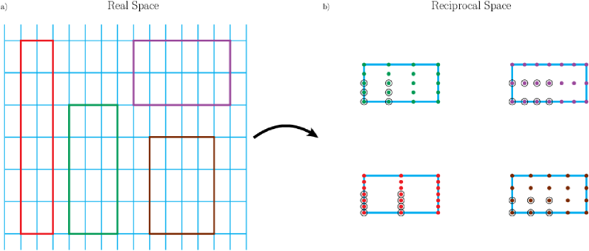
Figure 2: A 2D example of symmetry-preserving supercells and the $\mathbf{k}$-point grids that they would generate for a rectangular lattice. a) contains four symmetry preserving supercells of the primitive cell, shown in blue, with a volume factor of 12. In b) the primitive cell, blue cells, and the supercells have been mapped to reciprocal space and the grids that would have been generated from each supercell have been placed in a cell. The color of the grid points matches the color of the generating supercell. The circled points are the irreducible $\mathbf{k}$-points of each grid.

At a given volume factor (i.e., number of $\mathbf{k}$-points), the integer relations in Eq. (9) will yield multiple supercells for most lattices, a 2D example of these supercells is provided in Fig. 2(a). It is then neccessary to select one which defines the best $\mathbf{k}$-point grid. This is done by transforming each symmetry-preserving supercell to its corresponding $\mathbf{k}$-point grid generating vectors as in Eq. 3; see Fig. 2(b). We then search this set of grids for one that has optimal properties—a uniform distribution of points and the best symmetry reduction. To ensure the grid generating vectors are as short as possible we perform Minkowski reductionNguyen and Stehlé (2004), then sort the grids by the length of their shortest vector.

The most uniform grids will have the maximal shortest vector. We filter the grids so that none with a packing fraction of less then $0.3$ are considered. Each of the uniform grids is then symmetry reducedHart et al. in order to determine which has the fewest irreducible $\mathbf{k}$-points. Table 1 shows the length of the shortest vector and number of irreducible $\mathbf{k}$-points for the grids in Fig. 2(b). The grids are sorted first by the length of their shortest vector (eliminating the green and red grids) then by the number of irreducible $\mathbf{k}$-points such that the ideal grid appears at the top of the table, i.e., the grid generated by the brown supercell in Fig. 2(a).

grid	shortest vector length	number of irreducible $\mathbf{k}$-points
brown	$\frac{1}{6}$	6
purple	$\frac{1}{6}$	8
green	$\frac{1}{8}$	6
red	$\frac{1}{12}$	8

Table 1: Properties (length of shortest vector and number of irreducible $\mathbf{k}$-points) of the grids in Fig. 2

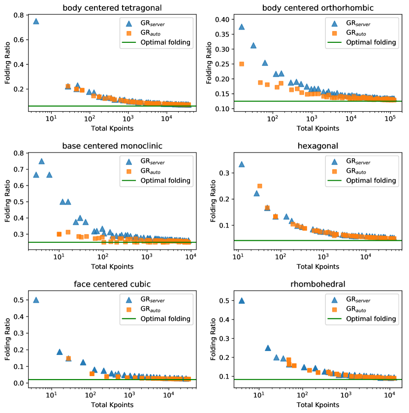
Figure 3: A comparison of the $GR_{\textrm{auto}}$ and $GR_{\textrm{server}}$ $\mathbf{k}$-point grids. For each grid th number of irreducible $\mathbf{k}$-points was divided by the total number of $\mathbf{k}$-points. This shows that both sets of grids offer similar folding at a given $\mathbf{k}$-point destiy and will have similar efficiencies.

It is also possible to offset the $\mathbf{k}$-point grid from the origin to improve the grids efficiency. The origin is not symmetrically equivalent to any other point in the grid; for example, including an offset makes it possible for the point at the origin to be mapped to other points in the grid, decreasing the number of irreducible $\mathbf{k}$-points. Different grids have different symmetry-preserving offsets that should be tested. For example, both simple cubic and face-centered cubic (fcc) grids have one possible offset that preserves the full symmetry of the cell, $(\frac{1}{2},\frac{1}{2},\frac{1}{2})$ (expressed as fractions of the grid generating vectors), while a body-centered-cubic lattice has no symmetry preserving offsets, and simple tetragonal has three symmetry preserving offsets. (For a full list of the symmetry-preserving offsets by lattice type, see the appendix.) The grid that has the fewest $\mathbf{k}$-points with a given offset is selected.

Not every volume factor will have a symmetry-preserving grid that is uniform. To ensure that a symmetry-preserving grid is found, it is necessary to include multiple volume factors in the search. The number of additional volume factors to search depends on the lattice type; in general, the search should continue until multiple candidate grids have been found. The best grid is then selected from these candidates.

II.4 Method Summary

The algorithm can be summarized in the following steps:

1. Identify the Niggli reduced cell of the user’s structure.

2. Generate the symmetry-preserving HNFs for the canonical form of the Niggli cell.

3. Map the resulting supercells to the original lattice using the Niggli-reduced basis as an intermediary.

4. Convert the supercells into $\mathbf{k}$-point grid generating vectors.

5. Perform Minkowski reduction on the grid generating vectors.

6. Sort the grid generating vectors by the length of their shortest vector.

7. Select the grids that maximize the length of the shortest vectors.

8. Use the symmetry group to reduce the selected grids to find the one with the fewest irreducible $\mathbf{k}$-points.

III Results

To test the above algorithm, we compared the $\mathbf{k}$-point grids it generates, $GR_{\textrm{auto}}$, to those generated by the $\mathbf{k}$-point severWisesa et al. (2016), $GR_{\textrm{server}}$ in two ways. First, we generated both grids over a range of $\mathbf{k}$-point densities for over 100 crystal lattices. These lattices were constructed for nine elemental systems—Al, Pd, Cu, W, V, K, Ti, Y, and Re—with supercells for the cubic systems having between 1–11 atoms per cell and supercells for the hexagonal close packed systems having between 2–14 atoms per cell. Additional test structures were selected from AFLOWCurtarolo et al. (2012). All tests were conducted without offsetting the grids from origin. We then plotted the resulting ratio of irreducible $\mathbf{k}$-points to total $\mathbf{k}$-points in each grid. Six representative examples of the results are shown in Fig. 3. These tests show that the $GR_{\textrm{auto}}$ grids should be very close in performance to $GR_{\textrm{server}}$ grids. Additionally, the tests show that convergence toward the ideal folding ratio is rapid for all lattice types.

The second test compared the total energy errors of MP (generated by AFLOW), $GR_{\textrm{auto}}$ and $GR_{\textrm{server}}$ grids in the same manner, and using the same methods, as done in our previous study of $GR$ gridsMorgan et al. (2018). We provide a brief review of that method here.

DFT calculations were performed using the Vienna Ab-initio Simulation Package 4.6 (VASP 4.6) Kresse and Hafner (1993); Kresse and Furthmüller (1996a); Kresse and Hafner (1994); Kresse and Furthmüller (1996b) on the nine monoatomic systems mentioned above using PAW PBE pseudopotentials.Blöchl (1994); Kresse and Joubert (1999) In order to isolate the errors from $\mathbf{k}$-point integeration, the different cells were crystallographically equivalent to single element cells. For MP grids, the target number of $\mathbf{k}$-points ranged from 10-10,000 unreduced $\mathbf{k}$-points, for $GR_{\textrm{server}}$ grids the range was 4–240,000 unreduced $\mathbf{k}$-points, and for $GR_{\textrm{auto}}$ the range was 8 to 415,000 unreduced $\mathbf{k}$-points. In total, we compared errors across more than 7000 total energy calculations. The energy taken as the error-free “solution” in our comparisons was the calculation with the highest $\mathbf{k}$-point density for each system. The total error convergence with respect to the $\mathbf{k}$-point density is shown in Fig. 4. The total error convergence with repsect to the number of irreducible $\mathbf{k}$-points were compared using loess regression, see Fig. 5. Ratios of these trend lines were then taken to determine the efficiency of each grid relative to the $GR_{\textrm{server}}$ grids (see Fig. 6).

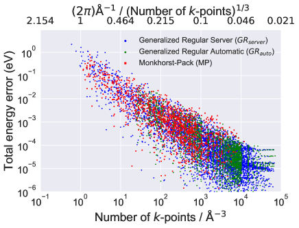
Figure 4: The total energy convergence with respect to total $\mathbf{k}$-point density for MP, $GR_{\textrm{auto}}$ and $GR_{\textrm{server}}$ grids. The top axis shows the linear $\mathbf{k}$-point spacing with a factor of 2$\pi$ included as part of the transformation to reciprocal space. This differs from the linear $\mathbf{k}$-point spacing usually used as input in DFT codes by a factor of 2$\pi$, i.e., to get the spacing used as input in codes divide the values here by 2$\pi$.

Figure 5: The total energy convergence with respect to irreducible $\mathbf{k}$-point density for MP, $GR_{\textrm{auto}}$ and $GR_{\textrm{server}}$ grids with loess regression applied.

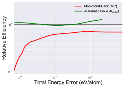
Figure 6: Along the $y$-axis are the ratios of the MP and $GR_{\textrm{auto}}$ efficiencies compared to the $GR_{\textrm{server}}$ grid efficiency (black horizontal line at $10^{0}$). Total energy error (per atom) is plotted along the $x$-axis and decreases to the left. MP grids are $\sim$60% less efficient than both $GR_{\textrm{auto}}$ and $GR_{\textrm{server}}$ grids at a target accuracy of 1meV/atom. The $GR_{\textrm{auto}}$ grids, however, outperform $GR_{\textrm{server}}$ grids at low densities but otherwise closely agree with $GR_{\textrm{auto}}$ grids.

From Figs. 5 and 6, it can be seen that $GR_{\textrm{auto}}$ grids are up to $\sim$10% more efficient and at worst $\sim$5% less efficient than $GR_{\textrm{server}}$ grids. Both sets of grids outperform MP grids by $\sim$60% at an accuracy target of 1 meV/atom. The runtime for the algorithm to generate $GR_{\textrm{auto}}$ grids at a $\mathbf{k}$-point density of 5000 (dense enough to achieve 1 meV/atom accuracy) was $\sim$3 seconds on average.

IV Conclusion

We have designed an algorithm that generates Generalized Regular (GR) grids “on the fly”. These $GR_{\textrm{auto}}$ grids are $\sim$60% more efficient than MP grids at an accuracy target of 1 meV/atom and have have similar efficiency to $GR_{\textrm{server}}$ gridsWisesa et al. (2016).

The algorithm is able to reduce the search space for $GR$ grids by only generating grids that preserve the symmetry of the input cell. The symmetry preserving grids are then filtered so that only the most efficient grid is returned to the user. For our test cases the average runtime of finding the optimal grid was $\sim$3 seconds. This algorithm has been implemented and is available for download at: https://github.com/msg-byu/GRkgridgen

V Acknowledgments

The authors are grateful to Tim Mueller, Georg Kresse and Martijn Marsman for helpful discussions. This work was supported by the Office of Naval Research (ONR MURI N00014-13-1-0635). The authors are grateful to C.S. Reese who helped with the loess regression and statistical analysis of the data shown Figs. 5 and 6.

VI Appendix

VI.1 Symmetry Preserving Offsets

The following is a table of the symmetry preserving offsets for each Bravais lattice expressed in terms of fractions of the primitive lattice vectors.

Simple Cubic	$\begin{pmatrix}\frac{1}{2},\;\frac{1}{2},\;\frac{1}{2}\end{pmatrix}$
Face Centered Cubic	$\begin{pmatrix}\frac{1}{2},\;\frac{1}{2},\;\frac{1}{2}\end{pmatrix}$
Body Centered Cubic	None
Hexagonal	$\begin{pmatrix}0,\;0,\;\frac{1}{2}\end{pmatrix}$
Rhombohedral	$\begin{pmatrix}0,\;0,\;\frac{1}{2}\end{pmatrix}$
Simple Tetragonal	$\begin{pmatrix}0,\;0,\;\frac{1}{2}\\ \frac{1}{2},\;\frac{1}{2},\;0\\ \frac{1}{2},\;\frac{1}{2},\;\frac{1}{2}\end{pmatrix}$
Body Centered Tetragonal	$\begin{pmatrix}0,\;0,\;\frac{1}{2}\end{pmatrix}$
Simple Orthorhombic	$\begin{pmatrix}0,\;0,\;\frac{1}{2}\\ 0,\;\frac{1}{2},\;0\\ \frac{1}{2},\;0,\;0\\ 0,\;\frac{1}{2},\;\frac{1}{2}\\ \frac{1}{2},\;0,\;\frac{1}{2}\\ \frac{1}{2},\;\frac{1}{2},\;0\\ \frac{1}{2},\;\frac{1}{2},\;\frac{1}{2}\end{pmatrix}$
Base Centered Orthorhombic	$\begin{pmatrix}0,\;0,\;\frac{1}{2}\\ 0,\;\frac{1}{2},\;0\\ 0,\;\frac{1}{2},\;\frac{1}{2}\end{pmatrix}$
Face Centered Orthorhombic	$\begin{pmatrix}\frac{1}{2},\;\frac{1}{2},\;\frac{1}{2}\end{pmatrix}$
Body Centered Orthorhombic	$\begin{pmatrix}0,\;0,\;\frac{1}{2}\\ 0,\;\frac{1}{2},\;0\\ \frac{1}{2},\;0,\;0\end{pmatrix}$
Simple Monoclinic	$\begin{pmatrix}0,\;0,\;\frac{1}{2}\\ 0,\;\frac{1}{2},\;0\\ \frac{1}{2},\;0,\;0\\ 0,\;\frac{1}{2},\;\frac{1}{2},\\ \frac{1}{2}\;0,\;\frac{1}{2},\\ \frac{1}{2},\;\frac{1}{2},\;0\\ \frac{1}{2},\;\frac{1}{2},\;\frac{1}{2}\end{pmatrix}$
Base Centered Monoclinic	$\begin{pmatrix}0,\;0,\;\frac{1}{2}\\ 0,\;\frac{1}{2},\;0\\ -\frac{1}{4},\;\frac{1}{2},\;0\\ -\frac{1}{4},\;\frac{1}{4},\;\frac{1}{2}\\ \frac{1}{4},\;\frac{1}{4},\;0\\ \frac{1}{4},\;\frac{1}{4},\;\frac{1}{2}\\ 0,\;\frac{1}{2},\;\frac{1}{2}\end{pmatrix}$
Triclinic	None

References

- Wisesa et al. (2016) P. Wisesa, K. A. McGill, and T. Mueller, Phys. Rev. B 93, 155109 (2016).
- Morgan et al. (2018) W. S. Morgan, J. J. Jorgensen, B. C. Hess, and G. L. Hart, Computational Materials Science 153, 424 (2018).
- Curtarolo et al. (2012) S. Curtarolo, W. Setyawan, G. L. Hart, M. Jahnatek, R. V. Chepulskii, R. H. Taylor, S. Wang, J. Xue, K. Yang, O. Levy, et al., Comput. Mat. Sci. 58, 218 (2012).
- Saal et al. (2013) J. E. Saal, S. Kirklin, M. Aykol, B. Meredig, and C. Wolverton, JOM 65, 1501 (2013).
- Jain et al. (2013) A. Jain, S. P. Ong, G. Hautier, W. Chen, W. D. Richards, S. Dacek, S. Cholia, D. Gunter, D. Skinner, G. Ceder, et al., APL Mat. 1, 011002 (2013).
- Digabel et al. (2009) S. L. Digabel, C. Tribes, and C. Audet, NOMAD user guide, Tech. Rep. G-2009-37 (Les cahiers du GERAD, Quebec, Canada, 2009).
- Landis et al. (2012) D. D. Landis, J. S. Hummelshøj, S. Nestorov, J. Greeley, M. Dułak, T. Bligaard, J. K. Nørskov, and K. W. Jacobsen, Comput. Sci. Eng. 14, 51 (2012).
- Hachmann et al. (2011) J. Hachmann, R. Olivares-Amaya, S. Atahan-Evrenk, C. Amador-Bedolla, R. S. Sánchez-Carrera, A. Gold-Parker, L. Vogt, A. M. Brockway, and A. Aspuru-Guzik, J. Phys. Chem. Lett. 2, 2241 (2011).
- Hummelshøj et al. (2012) J. S. Hummelshøj, F. Abild-Pedersen, F. Studt, T. Bligaard, and J. K. Nørskov, Angewandte Chemie 124, 278 (2012).
- De Jong et al. (2015a) M. De Jong, W. Chen, H. Geerlings, M. Asta, and K. A. Persson, Sci. Data 2 (2015a).
- De Jong et al. (2015b) M. De Jong, W. Chen, T. Angsten, A. Jain, R. Notestine, A. Gamst, M. Sluiter, C. K. Ande, S. Van Der Zwaag, J. J. Plata, et al., Sci. Data 2, 150009 (2015b).
- Cheng et al. (2015) L. Cheng, R. S. Assary, X. Qu, A. Jain, S. P. Ong, N. N. Rajput, K. Persson, and L. A. Curtiss, J. Phys. Chem. Lett. 6, 283 (2015).
- Gómez-Bombarelli et al. (2016) R. Gómez-Bombarelli, J. Aguilera-Iparraguirre, T. D. Hirzel, D. Duvenaud, D. Maclaurin, M. A. Blood-Forsythe, H. S. Chae, M. Einzinger, D.-G. Ha, T. Wu, et al., Nat. Mater. 15, 1120 (2016).
- Chan (2015) E. M. Chan, Chem. Soc. Rev. 44, 1653 (2015).
- Tada et al. (2014) T. Tada, S. Takemoto, S. Matsuishi, and H. Hosono, Inorg. Chem. 53, 10347 (2014).
- Pilania et al. (2013) G. Pilania, C. Wang, X. Jiang, S. Rajasekaran, and R. Ramprasad, Sci. Rep. 3 (2013).
- Yan et al. (2015a) J. Yan, P. Gorai, B. Ortiz, S. Miller, S. A. Barnett, T. Mason, V. Stevanović, and E. S. Toberer, Energy Environ. Sci. 8, 983 (2015a).
- Ramakrishnan et al. (2014) R. Ramakrishnan, P. O. Dral, M. Rupp, and O. A. Von Lilienfeld, Sci. Data 1, 140022 (2014).
- Hachmann et al. (2014) J. Hachmann, R. Olivares-Amaya, A. Jinich, A. L. Appleton, M. A. Blood-Forsythe, L. R. Seress, C. Roman-Salgado, K. Trepte, S. Atahan-Evrenk, S. Er, et al., Energy Environ. Sci. 7, 698 (2014).
- Lin et al. (2012) L.-C. Lin, A. H. Berger, R. L. Martin, J. Kim, J. A. Swisher, K. Jariwala, C. H. Rycroft, A. S. Bhown, M. W. Deem, M. Haranczyk, et al., Nat. Mater. 11, 633 (2012).
- Armiento et al. (2014) R. Armiento, B. Kozinsky, G. Hautier, M. Fornari, and G. Ceder, Phys. Rev. B 89, 134103 (2014).
- Senkov et al. (2015) O. Senkov, J. Miller, D. Miracle, and C. Woodward, Nat. Commun. 6 (2015).
- Greeley et al. (2006) J. Greeley, T. F. Jaramillo, J. Bonde, I. Chorkendorff, and J. K. Nørskov, Nat. Mater. 5, 909 (2006).
- Gautier et al. (2015) R. Gautier, X. Zhang, L. Hu, L. Yu, Y. Lin, T. O. Sunde, D. Chon, K. R. Poeppelmeier, and A. Zunger, Nat. Chem. 7, 308 (2015).
- Oliynyk and Mar (2017) A. O. Oliynyk and A. Mar, Accounts of chemical research (2017).
- Chen et al. (2012a) H. Chen, G. Hautier, A. Jain, C. Moore, B. Kang, R. Doe, L. Wu, Y. Zhu, Y. Tang, and G. Ceder, Chem. Mat. 24, 2009 (2012a).
- Hautier et al. (2011) G. Hautier, A. Jain, S. P. Ong, B. Kang, C. Moore, R. Doe, and G. Ceder, Chem. Mater. 23, 3495 (2011).
- Jähne et al. (2013) C. Jähne, C. Neef, C. Koo, H.-P. Meyer, and R. Klingeler, J. Mater. Chem. A 1, 2856 (2013).
- Moot et al. (2016) T. Moot, O. Isayev, R. W. Call, S. M. McCullough, M. Zemaitis, R. Lopez, J. F. Cahoon, and A. Tropsha, Materials Discovery 6, 9 (2016).
- Aydemir et al. (2016) U. Aydemir, J.-H. Pöhls, H. Zhu, G. Hautier, S. Bajaj, Z. M. Gibbs, W. Chen, G. Li, S. Ohno, D. Broberg, et al., J. Mat. Chem. A 4, 2461 (2016).
- Zhu et al. (2015) H. Zhu, G. Hautier, U. Aydemir, Z. M. Gibbs, G. Li, S. Bajaj, J.-H. Pöhls, D. Broberg, W. Chen, A. Jain, et al., J. Mat. Chem. C 3, 10554 (2015).
- Chen et al. (2016) W. Chen, J.-H. Pöhls, G. Hautier, D. Broberg, S. Bajaj, U. Aydemir, Z. M. Gibbs, H. Zhu, M. Asta, G. J. Snyder, et al., J. Mat. Chem. C 4, 4414 (2016).
- Ceder et al. (1998) G. Ceder, Y.-M. Chiang, D. Sadoway, M. Aydinol, Y.-I. Jang, and B. Huang, Nature 392, 694 (1998).
- Yan et al. (2015b) F. Yan, X. Zhang, G. Y. Yonggang, L. Yu, A. Nagaraja, T. O. Mason, and A. Zunger, Nat. Commun. 6 (2015b).
- Bende et al. (2017) D. Bende, F. R. Wagner, O. Sichevych, and Y. Grin, Angewandte Chemie 129, 1333 (2017).
- Mannodi-Kanakkithodi et al. (2017) A. Mannodi-Kanakkithodi, A. Chandrasekaran, C. Kim, T. D. Huan, G. Pilania, V. Botu, and R. Ramprasad, Mater. Today (2017).
- Sanvito et al. (2017) S. Sanvito, C. Oses, J. Xue, A. Tiwari, M. Zic, T. Archer, P. Tozman, M. Venkatesan, M. Coey, and S. Curtarolo, Sci. Adv. 3, e1602241 (2017).
- Yaghoobnejad Asl and Choudhury (2016) H. Yaghoobnejad Asl and A. Choudhury, Chem. Mater. 28, 5029 (2016).
- Hautier et al. (2013) G. Hautier, A. Miglio, G. Ceder, G.-M. Rignanese, and X. Gonze, Nat. Commun. 4, 2292 (2013).
- Bhatia et al. (2015) A. Bhatia, G. Hautier, T. Nilgianskul, A. Miglio, J. Sun, H. J. Kim, K. H. Kim, S. Chen, G.-M. Rignanese, X. Gonze, et al., Chem. Mater. 28, 30 (2015).
- Johannesson et al. (2002) G. H. Johannesson, T. Bligaard, A. V. Ruban, H. L. Skriver, K. W. Jacobsen, and J. K. Nørskov, Phys. Rev. Lett. 88, 255506 (2002).
- Stucke and Crespi (2003) D. P. Stucke and V. H. Crespi, Nano Lett. 3, 1183 (2003).
- Curtarolo et al. (2005) S. Curtarolo, D. Morgan, and G. Ceder, Calphad 29, 163 (2005).
- Matar et al. (2009) S. F. Matar, I. Baraille, and M. Subramanian, Chem. Phys. 355, 43 (2009).
- Ceder et al. (2011) G. Ceder, G. Hautier, A. Jain, and S. P. Ong, MRS Bulletin 36, 185 (2011).
- Sokolov et al. (2011) A. N. Sokolov, S. Atahan-Evrenk, R. Mondal, H. B. Akkerman, R. S. Sánchez-Carrera, S. Granados-Focil, J. Schrier, S. C. Mannsfeld, A. P. Zoombelt, Z. Bao, et al., Nat. Commun. 2, 437 (2011).
- Ulissi et al. (2017) Z. W. Ulissi, M. T. Tang, J. Xiao, X. Liu, D. A. Torelli, M. Karamad, K. Cummins, C. Hahn, N. S. Lewis, T. F. Jaramillo, et al., ACS Catal. 7, 6600 (2017).
- Levy et al. (2009) O. Levy, R. V. Chepulskii, G. L. Hart, and S. Curtarolo, JACS 132, 833 (2009).
- Ma et al. (2013) X. Ma, G. Hautier, A. Jain, R. Doe, and G. Ceder, J. Electrochem. Soc. 160, A279 (2013).
- Yang et al. (2012) K. Yang, W. Setyawan, S. Wang, M. B. Nardelli, and S. Curtarolo, Nat. Mater. 11, 614 (2012).
- Chen et al. (2012b) H. Chen, G. Hautier, and G. Ceder, JACS 134, 19619 (2012b).
- Kirklin et al. (2013) S. Kirklin, B. Meredig, and C. Wolverton, Advanced Energy Materials 3, 252 (2013).
- Monkhorst and Pack (1976) H. J. Monkhorst and J. D. Pack, Phys. Rev. B 13, 5188 (1976).
- Moreno and Soler (1992) J. Moreno and J. M. Soler, Phys. Rev. B 45, 13891 (1992).
- Note (1) Note that the determinant of determines the number of -points in the Brillouin zone.
- Kr̆ivý and Gruber (1976) I. Kr̆ivý and B. Gruber, Acta Crystallogr. A 32 (1976).
- (57) A. Santoro and A. D. Mighell, Acta Crystallogr. A 26, 124, https://onlinelibrary.wiley.com/doi/pdf/10.1107/S0567739470000177 .
- Grosse-Kunstleve et al. (2004) R. W. Grosse-Kunstleve, N. K. Sauter, and P. D. Adams, Acta Crystallogr. A 60, 1 (2004).
- edited by Theo Hahn (2002) edited by Theo Hahn, International tables for crystallography. Volume A, Space-group symmetry (Fifth, revised edition. Dordrecht ; London : Published for the International Union of Crystallography by Kluwer Academic Publishers, 2002., 2002).
- Nguyen and Stehlé (2004) P. Q. Nguyen and D. Stehlé, in Algorithmic Number Theory, edited by D. Buell (Springer Berlin Heidelberg, Berlin, Heidelberg, 2004) pp. 338–357.
- (61) G. L. W. Hart, J. Jorgensen, W. M. Morgan, and R. W. Forcade, arXiv:1809.10261 .
- Note (2) For some lattices no symmetry preserving offsets exist. In these cases using an offset that does not preserve the full symmetry can be beneficial. For example, a body centered cubic system with an offset of can sometimes offer better folding than the same grid with no offset.
- Kresse and Hafner (1993) G. Kresse and J. Hafner, Phys. Rev. B 47, 558 (1993).
- Kresse and Furthmüller (1996a) G. Kresse and J. Furthmüller, Comput. Mat. Sci. 6, 15 (1996a).
- Kresse and Hafner (1994) G. Kresse and J. Hafner, Phys. Rev. B 49, 14251 (1994).
- Kresse and Furthmüller (1996b) G. Kresse and J. Furthmüller, Phys. Rev. B 54, 11169 (1996b).
- Blöchl (1994) P. E. Blöchl, Phys. Rev. B 50, 17953 (1994).
- Kresse and Joubert (1999) G. Kresse and D. Joubert, Phys. Rev. B 59, 1758 (1999).