Spontaneous Josephson $\pi$ Junctions with Topological Superconductors

Abstract

We study a junction between two time-reversal-invariant topological superconductors and show this system goes through a series of multiple transitions between a $0$-junction phase, where the free energy has its minimum for a superconducting phase difference of zero, and a $\pi$-junction phase, where the free energy has its minimum for a superconducting phase difference of $\pi$. These transitions occur in the absence of Coulomb blockade or magnetic impurities. Rather, they are driven by the spin-orbit coupling in the junction, and can be probed, for example, by measuring the tunneling density of states or the critical current as a function of the junction’s length or its Fermi velocity.

I Introduction

Josephson $\pi$-junctions have been studied extensively in recent decades (Cleuziou et al., 2006; Kulik, 1966; Buzdin and Panyukov, 1982; Ryazanov et al., 2001; Kontos et al., 2002; Schulz et al., 2000; De Franceschi et al., 2010; Zaikin, 2004; Spivak and Kivelson, 1991). Unlike the more common Josephson $0$-junctions, where the free energy is minimized by a phase difference of $\phi=0$, these are junctions in which the free energy is minimized by a phase difference of $\phi=\pi.$

An important question is whether a $\pi$ junction can spontaneously form, in the absence of magnetic fields, in a junction between two topological superconductors. In the case of trivial superconductors, it has been established that a superconductor - quantum dot - superconductor (S-QD-S) junction can exhibit $\pi$-junction behavior as a result of Coulomb interaction in the QD (Glazman and Matveev, 1989; Spivak and Kivelson, 1991; Yeyati et al., 1997; Rozhkov et al., 2001; Zaikin, 2004; Siano and Egger, 2004; Choi et al., 2004; Sch, ).

Recently, Josephson junctions with two time-reversal-invariant topological superconductors (TRITOPSs) have also been studied (Zhang et al., 2013; Liu et al., 2014; Zhang and Kane, 2014; Kane and Zhang, 2015; Gong et al., 2016; Camjayi et al., 2017; Arrachea et al., ). Such a topological superconductor (Schnyder et al., 2008; Qi et al., 2009, 2010; Qi and Zhang, 2011; Haim and Oreg, 2019) hosts protected pairs of Majorana zero modes at each of its boundaries while maintaining a bulk gap. It was shown that these Majorana zero modes can form an effective spin which in turn screens the spin of the QD, thereby avoiding the $\pi$-junction fate of conventional superconductors (Camjayi et al., 2017).

In this paper, we show that a Josephson junction with two TRITOPSs can nevertheless be driven into the $\pi$-junction phase via a different mechanism. Specifically, the system goes through multiple transitions between 0-junction and $\pi$-junction behavior, as a function of the rotation angle acquired by the electron’s spin as it passes the junction. This rotation is caused by spin-orbit coupling, and depends on the junction’s length and the Fermi velocity.

The mechanism behind the formation of the $\pi$ junction is intimately related to the defining topological property of the TRITOPS phase, namely the sign difference that exists between the pairing potentials of positive- and negative-helicity modes Qi et al. (2010); Haim and Oreg (2019). As we show below, in the presence of spin-orbit coupling in the junction, this sign difference translates into a relative $\pi$ phase difference between the superconductors on the two sides of the junction (see Fig. 3).

We begin by studying a low-energy model, which provides a simple physical picture, and allows for an analytical expression describing the equilibrium phase difference. We then move on to study the junction numerically using a microscopic lattice model. We use it to calculate the tunneling density of states in the junction, and the critical current; these can serve as experimental signatures of the $0$-$\pi$ transitions.

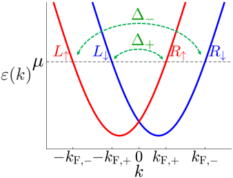
(a)

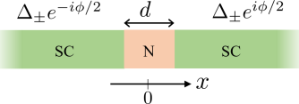
(b)

Figure 1: (a) Electronic spectrum of the model described in Eq. (8). Close to the Fermi level, it can be described by four linearly-dispersing modes. The positive-helicity modes experience a pairing potential, $\Delta_{+}$, while the negative-helicity modes experience a pairing potential, $\Delta_{-}$ [see Eq. (1)]. The time-reversal-invariant topological superconductor (TRITOPS) phase is realized when $\Delta_{+}\Delta_{-}<0$. (b) Josephson junction between two TRITOPSs.

II Low-energy model

A uniform TRITOPS can be described, at low energies, by the Hamiltonian (Qi et al., 2010; Haim et al., 2016; Haim and Oreg, 2019)

$$\begin{split}H_{0}=\int_{-\infty}^{\infty}{\rm d}x&\Big{\{}-iv\sum_{s=\uparrow\downarrow}\left[R_{s}^{\dagger}\partial_{x}R_{s}-L_{s}^{\dagger}\partial_{x}L_{s}\right]\\ &+\left[\Delta_{+}R_{\uparrow}^{\dagger}L_{\downarrow}^{\dagger}+\Delta_{-}L_{\uparrow}^{\dagger}R_{\downarrow}^{\dagger}+{\rm h.c.}\right]\Big{\}},\end{split}$$ (1)

where $R_{s}(x)$ [$L_{s}(x)$] is a field describing a right- (left-) moving electron with spin $s=\uparrow,\downarrow$ and velocity $v$. The pairing potential $\Delta_{+}$ describes pairing between modes of positive helicity ($R_{\uparrow}$ and $L_{\downarrow}$), while $\Delta_{-}$ describes pairing between modes of negative helicity ($L_{\uparrow}$ and $R_{\downarrow}$) [see Fig. 1(a)].

We are interested in systems obeying time-reversal symmetry, implemented by

$$R_{s}\to i\sigma_{ss^{\prime}}^{y}L_{s^{\prime}}\hskip 10.00002pt;\hskip 10.00002ptL_{s}\to i\sigma_{ss^{\prime}}^{y}R_{s^{\prime}}\hskip 10.00002pt;\hskip 10.00002pti\to-i,$$ (2)

where $\{\sigma^{\alpha=x,y,z}\}$ are the Pauli matrices. This constrains the pairing potentials to be real, $\Delta_{\pm}\in\mathbb{R}$. It can be shown that $H_{0}$ is in the topological phase, with a pair of Majorana zero modes at each end, when the topological invariant $\mathcal{Q}=\rm{sgn}(\Delta_{+}\Delta_{-})$ is negative (Qi et al., 2010; Haim and Oreg, 2019), namely when the positive-helicity modes experience a pairing potential with opposite sign to that of the negative-helicity modes.

Notice that $H_{0}$ obeys a spin-rotation symmetry, $[H_{0},S_{z}]=0$, where $S_{z}=\int{\rm d}x\sigma_{ss^{\prime}}^{z}(R_{s}^{\dagger}R_{s^{\prime}}+L_{s}^{\dagger}L_{s^{\prime}})$ . This is not a fundamental symmetry of the TRITOPS phase. It is rather an emergent symmetry of its long-wavelength description. As we will see below, the junction generally breaks this symmetry, which will prove crucial for obtaining the $\pi$-junction phase.

We now consider a superconductor - normal-metal - superconductor (SNS) junction with two TRITOPSs. To this end, we promote $\Delta_{\pm}$ to have the following spatial dependence,

$$\Delta_{\pm}(x)=\Delta_{\pm}^{0}\theta(|x|-d/2)e^{i\frac{\phi}{2}{\rm sgn}(x)},$$ (3)

where $\theta(x)$ is the Heaviside step function, $d$ is the junction’s length, and $\phi$ is the phase difference across the junction [see Fig. 1(b)]. Furthermore, we allow for spin-orbit coupling, as well as backscattering, inside the junction, such that the Hamiltonian for the entire system is $H=H_{0}+H_{{\rm so}}+H_{{\rm bs}}$, with

$$\begin{split}H_{{\rm so}}=&U_{{\rm so}}\int_{-d/2}^{d/2}{\rm d}x\left(R_{\uparrow}^{\dagger}R_{\downarrow}-L_{\uparrow}^{\dagger}L_{\downarrow}\right)+{\rm h.c.,}\\ H_{{\rm b}}=&V_{\rm b}^{\prime}\sum_{s=\uparrow\downarrow}\left[R_{s}^{\dagger}(0)+L_{s}^{\dagger}(0)\right]\left[R_{s}(0)+L_{s}(0)\right].\end{split}$$ (4)

Here, $H_{{\rm so}}$ is a spin-orbit coupling term, responsible for rotation of the spin as the electron traverses the junction, and $H_{{\rm b}}$ is a delta-potential barrier that controls the transparency of the junction . Both terms are allowed by time-reversal symmetry and therefore will generally be present.

To obtain the ground-state energy of the junction, we first calculate the spectrum of Andreev bound states, which is done by solving the single-particle Schrödinger equation for $H$. In the special case of $\Delta_{+}^{0}=-\Delta_{-}^{0}\equiv\Delta$, and $d\ll v/\left|\Delta\right|$, one obtains (Mellars and Béri, 2016; Kwon et al., 2004)

$$\varepsilon_{\pm}(\phi)=\sqrt{\tau}\Delta\cos\left(\frac{\phi\pm\beta_{{\rm so}}}{2}\right)\,\,\,\,;\,\,\,\,\beta_{{\rm so}}\equiv\frac{2\left|U_{{\rm so}}\right|d}{v},$$ (5)

where $\tau=1/[1+(V_{\rm b}^{\prime}/v)^{2}]$ is the transmission probability of the junction in the normal state, and $\beta_{{\rm so}}$ is the spin-rotation angle acquired as the electron traverses the junction. Together with their particle-hole partners, the excitation spectrum is given by $\left\{\varepsilon_{+}(\phi),\varepsilon_{-}(\phi),-\varepsilon_{+}(\phi),-\varepsilon_{-}(\phi)\right\}$, shown in Figs. 2(a,b), for $\beta_{{\rm so}}=\pi/3$ and $\beta_{{\rm so}}=2\pi/3$, respectively .

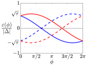
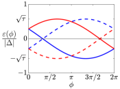
(a)	(b)
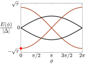
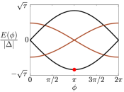
(c)	(d)

Figure 2: (a,b) Single-particle excitation spectrum of the Josephson junction described in Eqs. (1,3,4), as a function of phase bias, for different spin-rotation angle: (a) $\beta_{{\rm so}}=\pi/3$, and (b) $\beta_{{\rm so}}=2\pi/3$. Excitation energies marked by a solid and dashed line are related by particle-hole symmetry. (c,d) Many-body energy spectra, corresponding to (a,b), respectively. In (c), the global ground state is at $\phi_{{\rm eq}}=0$, while in (d) the global ground state is at $\phi_{{\rm eq}}=\pi$. This transition from a $0$-junction to a $\pi$-junction occurs abruptly at $\beta_{{\rm so}}=\pi/2$ [see Eq. (7)]. Energy states marked in brown (black) have even (odd) Fermion parity.

For a fixed phase difference, $\phi$, the ground-state energy is obtained by summing the negative excitation energies,

$$E_{{\rm gs}}(\phi)=-[\left|\varepsilon_{+}(\phi)\right|+\left|\varepsilon_{-}(\phi)\right|]/2.$$ (6)

If the phase difference is not set externally, it is determined, at zero temperature, by minimization of $E_{{\rm gs}}(\phi)$. From Eqs. (5) and (6) one then obtains the phase difference at thermal equilibrium,

$$\phi_{{\rm eq}}=\begin{cases}0,&|\tan(\beta_{{\rm so}}/2)|<1\\ \pi,&|\tan(\beta_{{\rm so}}/2)|>1.\end{cases}$$ (7)

As $\beta_{{\rm so}}$ is varied, the system goes through a series of transitions between a $0$-junction and a $\pi$-junction, at $\beta_{{\rm so}}=\pi(1/2+N)$, for integer $N$. This can be achieved by tuning the length of the junction, $d$, or the velocity, $v$, which generally depends on the chemical potential. Figures 2(c,d) present the four lowest many-body energies, obtained by summing the single-particle excitation energies according to their occupation, for $\beta_{{\rm so}}=\pi/3$ and $\beta_{{\rm so}}=2\pi/3$. In the former case the minimal energy is obtained for $\phi_{{\rm eq}}=0$, while in the latter it is obtained for $\phi_{{\rm eq}}=\pi$.

In the case of finite temperature, $T,$ the equilibrium phase is determined by minimizing the free energy, $F(\phi)=-T\sum_{p=\pm}\ln\{2\cosh[\varepsilon_{p}(\phi)/2T]\}$, instead of the ground-state energy. Within the limits of validity of Eq. (5), one can check that this does not affect the result for $\phi_{{\rm eq}}$, Eq. (7) .

Finally, while the spectrum in Eq. (5) was calculated under the simplifying assumptions, $\Delta_{+}=-\Delta_{-}=\Delta$ and $d\ll v/|\Delta|$, its qualitative features are universal (Zhang and Kane, 2014; Mellars and Béri, 2016). Specifically, the level crossings at $\phi=0,\pi$ are protected by time-reversal symmetry, and the crossings at zero energy are protected by particle-hole symmetry .

III Physical picture

The above results can be intuitively understood from the low-energy description of the TRITOPS phase, Eq. (1). In the absence of spin-orbit coupling in the junction ($\beta_{{\rm so}}=0$), the Josephson junction decouples into two separate junctions: one involving the positive-helicity modes (with pairing potential $\Delta_{+}$), and one involving the negative-helicity modes (with pairing potential $\Delta_{-}$), as depicted in Fig. 3(a). The Josephson coupling across the junction then seeks to align the phases of $\Delta_{\pm}(x<0)$ with the phases of $\Delta_{\pm}(x>0)$, respectively, which is achieved when $\phi=0$.

For a non-vanishing spin-orbit coupling in the junction, on the other hand, the electron’s spin rotates by an angle $\beta_{{\rm so}}$ as it traverses the junction, causing modes of positive and negative helicities to mix. In the special case of $\beta_{{\rm so}}=\pi$, modes of positive helicity are perfectly converted to mode of negative helicity and vice versa, as depicted in Fig. 3(b). The Josephson coupling now seeks to align the phases of $\Delta_{\pm}(x<0)$ with those of $\Delta_{\mp}(x>0)$, respectively. Importantly, since in the TRITOPS phase $\Delta_{+}\Delta_{-}<0$, this translates to having $\phi=\pi$. The transition between these two cases occurs at $\beta_{{\rm so}}=\pi/2$ [See Eq. (7)].

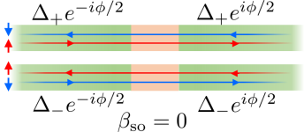
(a)

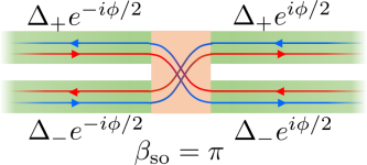
(b)

Figure 3: (a) In the absence of spin rotation in the junction, modes of positive and negative helicity do not mix. The Josephson coupling therefore tends to aligns the phases of $\Delta_{\pm}(x<0)$ with those of $\Delta_{\pm}(x>0)$, respectively, resulting in $\phi_{{\rm eq}}=0$. (b) At the other extreme, when the spin-rotation angle is $\beta_{{\rm so}}=\pi$, modes of positive (negative) helicity are converted to modes of negative (positive) helicity. Josephson coupling then tends to align the phases of $\Delta_{\pm}(x<0)$ with those of $\Delta_{\mp}(x>0)$, respectively. In the TRITOPS phase, where $\Delta_{+}\Delta_{-}<0$, this means $\phi_{{\rm eq}}=\pi.$

IV Experimental signature

The transition between a $0$-junction and a $\pi$-junction induces an abrupt change in the system’s physical observables, as in a first-order phase transition. Below, we focus on the behavior of the tunneling density of states and the critical current, and propose these can serve as experimental signatures of the transition.

We wish to study the Josephson junction beyond the simplifying assumptions leading to Eq. (5). To this end, we consider a lattice model of a TRITOPS and analyze it numerically. For a uniform TRITOPS, the Hamiltonian is given by (Zhang et al., 2013)

$$\begin{split}H_{0}^{{\rm Latt}}=&\sum_{n}\bigg{\{}-\mu\boldsymbol{\boldsymbol{c}}_{n}^{\dagger}\boldsymbol{\boldsymbol{c}}_{n}-\left[\boldsymbol{\boldsymbol{c}}_{n}^{\dagger}\left(t+iu\sigma_{z}\right)\boldsymbol{\boldsymbol{c}}_{n+1}+{\rm h.c.}\right]\\ &+\left[\frac{1}{2}\Delta_{0}\boldsymbol{\boldsymbol{c}}_{n}^{\dagger}i\sigma_{y}\boldsymbol{\boldsymbol{c}}_{n}^{\dagger{\rm T}}+\Delta_{1}\boldsymbol{\boldsymbol{c}}_{n}^{\dagger}i\sigma_{y}\boldsymbol{\boldsymbol{c}}_{n+1}^{\dagger{\rm T}}+{\rm h.c.}\right]\bigg{\}},\end{split}$$ (8)

where $\boldsymbol{\boldsymbol{c}}_{n}^{\dagger}=(c_{n\uparrow}^{\dagger},c_{n\downarrow}^{\dagger})$, and $c_{ns}^{\dagger}$ creates an electron on site $n$ with spin $s$. Here, $\mu$ is the chemical potential, $t$ is a hopping parameter, $u$ is the spin-orbit coupling coefficient, and $\Delta_{{\rm 0}}$ and $\Delta_{1}$ are singlet pairing potentials describing on-site and nearest-neighbor pairing, respectively. The system is in the topological phase when (Zhang et al., 2013) $2\left|u\right|\sqrt{1-\left[\Delta_{0}/(2\Delta_{1})\right]^{2}}>|\mu-t\Delta_{0}/\Delta_{1}|$.

Before proceeding, it is instructive to relate the lattice Hamiltonian, Eq. (8), to the low-energy Hamiltonian of Eq. (1). This can be done, in the weak pairing limit , by linearizing the spectrum of $H_{0}^{{\rm Latt}}$ near the Fermi momenta, $a_{0}k_{{\rm F},\pm}=\mp\lambda+\cos^{-1}\left[-\mu/(2w)\right]$, where $t=w\cos(\lambda)$, $u=w\sin(\lambda)$, and $a_{0}$ is the lattice constant [see also Fig. 1(a)]. The pairing potentials in the linearized model, Eq. (1), are then given by $\Delta_{\pm}=\Delta_{0}+2\Delta_{1}\cos(a_{0}k_{{\rm F},\pm})$, and the velocity is $v=a_{0}\sqrt{4w^{2}-\mu^{2}}.$

As before, in order to simulate a Josephson junction, we take the pairing potentials to depend on position according to $\Delta_{0,1}(n)=\Delta_{0,1}\theta(|na_{0}|-d/2)\exp\left[i{\rm sgn}(n)\phi/2\right]$. To account for spin rotation inside the junction, we include a spin-orbit coupling term in a perpendicular direction to the one in the bulk. This is done by letting $u$, in Eq. (8), vanish inside the junction, and instead adding a term ,

$$\begin{split}H_{{\rm so}}^{{\rm Latt}}=iu_{{\rm so},{\rm J}}\sum_{\left|na\right|<d/2}&\left[\boldsymbol{\boldsymbol{c}}_{n}^{\dagger}\sigma_{x}\boldsymbol{\boldsymbol{c}}_{n+1}-{\rm h.c.}\right]\end{split}.$$ (9)

For small $u_{{\rm so,J}},\mu$, the resulting spin rotation angle is $\beta_{{\rm so}}\simeq u_{{\rm so,J}}d/(a_{0}t)$. Finally, backscattering is accounted for by $H_{{\rm b}}^{{\rm Latt}}=V_{{\rm b}}\boldsymbol{c}_{0}^{\dagger}\boldsymbol{c}_{0}$, such that altogether the Hamiltonian is given by $H^{{\rm Latt}}=H_{0}^{{\rm Latt}}+H_{{\rm so}}^{{\rm Latt}}+H_{{\rm b}}^{{\rm Latt}}.$

To analyze $H^{{\rm Latt}}$, we first rewrite it in a Bogoliubov-de Gennes form, $H^{{\rm Latt}}=\frac{1}{2}\sum_{nn^{\prime}}\psi_{n}^{\dagger}\mathcal{H}_{nn^{\prime}}\psi_{n^{\prime}}$, where $\psi_{n}^{\dagger}=(\boldsymbol{c}_{n}^{\dagger},\boldsymbol{c}_{n}^{\rm T})$, and accordingly $\mathcal{H}_{nn^{\prime}}$ is a $4\times 4$ matrix that includes spin and particle-hole degrees of freedom. The tunneling density of states inside the junction is then given by

$$\rho_{{\rm J}}(\omega)=-\frac{1}{\pi}{\rm Im}\sum_{|na_{0}|<d/2}{\rm Tr}G_{nn}^{R}(\omega),$$ (10)

where $G^{R}(\omega)=\left[\omega+i\eta-\mathcal{H}\right]^{-1}$ is the retarded Green function . As a preliminary, we calculate the tunneling density of states as a function of the phase difference, $\phi$, for fixed system parameters in the TRITOPS phase. The results are presented in Figs. 4(a,b) for $u_{{\rm so,J}}=0.2$ and $u_{{\rm so,J}}=0.6$, respectively, with $d=5a_{0}$, and $V_{{\rm b}}=1$. This should be compared with the excitation spectrum given in Eq. (5) and shown in Figs. 2(a,b). Notice that while the latter was obtained from the linearized model in the limit of a short junction and for the special case $\Delta_{+}=-\Delta_{-}$, the qualitative features of the spectrum are retained.

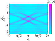
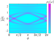
(a)	(b)
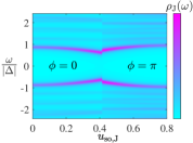
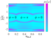
(c)	(d)

Figure 4: Density of states inside the junction, $\rho_{{\rm J}}(\omega)$, in arbitrary units, for fixed parameters, $t=2$, $u=1$, $\mu=-1.5$, $\Delta_{{\rm 0}}=0.2$, $\Delta_{{\rm 1}}=1$, and $V_{{\rm b}}=1$ [see Eqs. (8,9)]. Each of the superconductors is of length $L_{{\rm sc}}=100a_{0}$. In (a,b), $\rho_{{\rm J}}(\omega)$ is presented versus the phase difference, $\phi$, for junction length $d=5a_{0}$, and for (a) $u_{{\rm so,J}}=0.2$, (b) $u_{{\rm so,J}}=0.6$. In (c,d), $\rho_{{\rm J}}(\omega)$ is presented versus $u_{{\rm so,J}}$, for (c) $d=5a_{0}$, and (d) $d=9a_{0}$. The transitions between the $0$-junction and the $\pi$-junction are manifested in a non-analytic behavior of $\rho_{{\rm J}}(\omega)$. The frequency, $\omega$, is normalized by the bulk gap, $|\Delta|=0.248$.

Next, we wish to examine the transition between a 0-junction and a $\pi$-junction when tuning one of the system parameters. We vary the spin-orbit-coupling coefficient in the junction, $u_{{\rm so,J}}$. For each value of $u_{{\rm so,J}}$, we numerically search for the phase, $\phi_{{\rm eq}}$ , which minimizes the ground state energy of $H^{{\rm Latt}}$,

$$E_{{\rm gs}}(\phi)=\frac{1}{2}\sum_{\varepsilon_{\nu}<0}\varepsilon_{\nu}(\phi),$$ (11)

where $\left\{\varepsilon_{\nu}(\phi)\right\}_{\nu}$ are the eigenvalues of $\mathcal{H}$. Figures 4(c,d) present $\rho_{{\rm J}}(\omega;\phi_{{\rm eq}})$ for two different junction’s length, $d=5a_{0}$ and $d=9a_{0}$, respectively. As expected, the density of states exhibits non-analytic behavior at the transitions. This should be compared with Eqs. (5,7), which suggest that, at the transition, the subgap excitations, $\varepsilon_{\pm}=\sqrt{\tau/2}\Delta$, are continuous, but have a jump in their derivative.

A signature of the transition can also be found in measurement of the critical current, given by $I_{{\rm c}}={\rm max}_{\phi}[|I_{{\rm s}}(\phi)|]$, where $I_{{\rm s}}(\phi)=2e{\rm d}F(\phi)/{\rm d}\phi$ is the supercurrent for fixed $\phi$. Within the limits of validity of Eqs. (5,6), and for zero temperature, one arrives at $I_{c}=e\sqrt{\tau}|\Delta|\max\left\{\cos^{2}(\beta_{{\rm so}}/2),\sin^{2}(\beta_{{\rm so}}/2)\right\}$. Importantly, at the transition points, $\beta_{{\rm so}}=\pi(1/2+N)$, the critical current has its minimum, accompanied by a discontinuity in ${\rm d}I_{{\rm c}}/{\rm d}\beta_{{\rm so}}$. In Figs. 5(a,b) we present $I_{{\rm c}}$ versus the junction’s spin-orbit coupling, for different temperatures, calculated from the lattice model, Eqs. (8,9), for the same parameters as in Figs. 4(c,d), respectively. Indeed, $I_{{\rm c}}$ has a non-analytic minimum at the transitions.

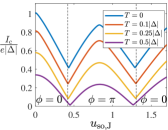
(a)

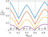
(b)

Figure 5: (a,b) Critical current as a function of the spin-orbit coupling in the junction, for different temperatures. System parameters are the same as in Figs. 4(c,d), respectively. Vertical dashed lines mark the zero-temperature transitions between a 0 junction and a $\pi$ junction. At these points, $I_{{\rm c}}$ has a minimum and a discontinuity in its derivative.

V Discussion

We have shown that a $\pi$ junction can spontaneously form, in the absence of magnetic fields, between two topological superconductors. Unlike its topologically-trivial counter part, this Josephson $\pi$ junction does not form as a result of Coulomb blockade. Instead, it is driven by spin-orbit coupling in the junction. When varying the rotation angle acquired by the electron’s spin as it passes the junction, the system goes through multiple transitions between a $0$-junction, where the phase difference at thermal equilibrium is $\phi_{{\rm eq}}=0$, and a $\pi$-junction, where the phase difference is $\phi_{{\rm eq}}=\pi$.

Experimentally, these transitions should be observable when one avoids fixing the phase externally (for instance using a flux loop), but rather let the phase be determined based on energetic considerations. In particular, if the TRITOPSs in the junction are realized by a semiconductor-superconductor heterostructure (Nakosai et al., 2013; Wong and Law, 2012; Zhang et al., 2013; Keselman et al., 2013; Gaidamauskas et al., 2014; Haim et al., 2014; Klinovaja et al., 2014; Klinovaja and Loss, 2014; Schrade et al., 2015; Danon and Flensberg, 2015; Haim et al., 2016; Thakurathi et al., 2018; Ebisu et al., 2016; Hsu et al., 2018; Wang et al., 2018; Yan et al., 2018; Baba et al., 2018), it is important to avoid direct coupling between the parent superconductors, as this can give rise to a Josephson coupling that competes with the mechanism studied above.

We propose measuring the density of states in the junction as a way of observing the transitions. This can be done, for example, using a weakly-coupled metallic lead or an STM probe. The density of states exhibits non-analytic behavior at the transitions [see Figs. 4(a,b)]. To tune across the transition, one has to vary parameters which control the spin rotation angle in the junction, such as the junction’s length or the electron velocity.

As an alternative signature, one can force current through the junction and measure the critical current. As one tunes across a transition point, the critical current exhibits a sharp dip, accompanied by a discontinuity in its first derivative. Similar behavior has been recently predicted (Pientka et al., 2017) in a different context, in a planar Josephson junction. There, a magnetic field drives a first-order phase transition, where the phase difference changes discontinuously. Note that, in their case, the phase on either side of the transition is not limited to the values $\{0,\pi\}$.

For a Josephson junction realized in a semiconductor-superconductor heterostructures, one can estimate the junction’s length needed to observe a transition. Assuming a spin-orbit coupling scale of $U_{{\rm so}}\sim 0.1{\rm meV}$, and electron velocity of $v\sim 10^{5}m/s$, the first transition occurs at a length $d\sim 500{\rm nm}$ [see Eqs. (5,7)].

A particularly appealing system for demonstrating the effect is a 2d topological insulator where each edge is coupled to a conventional superconductors Keselman et al. (2013); Klinovaja et al. (2014), thereby realizing a similar scenario to the one depicted in Fig. 3. For each side of the junction to be in the TRITOPS phase, the superconductors on the upper and lower edges are tuned to have a relative $\pi$ phase difference. This, however, does not yet determine the relative phase between the superconductors on the left and right. The prediction of this paper is that the latter will go through a series of transitions between $0$ and $\pi$ as a function of the spin-rotation angle in the junction.

References

- Cleuziou et al. (2006) J.-P. Cleuziou, W. Wernsdorfer, V. Bouchiat, T. Ondarçuhu, and M. Monthioux, Nat. Nano. 1, 53 (2006).
- Kulik (1966) I. Kulik, Sov. Phys. JETP 22, 841 (1966).
- Buzdin and Panyukov (1982) A. I. Buzdin and S. Panyukov, JETP Lett 35, 147 (1982).
- Ryazanov et al. (2001) V. V. Ryazanov, V. A. Oboznov, A. Y. Rusanov, A. V. Veretennikov, A. A. Golubov, and J. Aarts, Phys. Rev. Lett. 86, 2427 (2001).
- Kontos et al. (2002) T. Kontos, M. Aprili, J. Lesueur, F. Genêt, B. Stephanidis, and R. Boursier, Phys. Rev. Lett. 89, 137007 (2002).
- Schulz et al. (2000) R. R. Schulz, B. Chesca, B. Goetz, C. Schneider, A. Schmehl, H. Bielefeldt, H. Hilgenkamp, J. Mannhart, and C. Tsuei, Appl. Phys. Lett. 76, 912 (2000).
- De Franceschi et al. (2010) S. De Franceschi, L. Kouwenhoven, C. Schönenberger, and W. Wernsdorfer, Nat. Nano. 5, 703 (2010).
- Zaikin (2004) A. D. Zaikin, Low Temp. Phys. 30, 568 (2004).
- Spivak and Kivelson (1991) B. I. Spivak and S. A. Kivelson, Phys. Rev. B 43, 3740 (1991).
- Glazman and Matveev (1989) L. Glazman and K. Matveev, JETP Lett 49, 659 (1989).
- Yeyati et al. (1997) A. L. Yeyati, J. C. Cuevas, A. López-Dávalos, and A. Martín-Rodero, Phys. Rev. B 55, R6137 (1997).
- Rozhkov et al. (2001) A. V. Rozhkov, D. P. Arovas, and F. Guinea, Phys. Rev. B 64, 233301 (2001).
- Siano and Egger (2004) F. Siano and R. Egger, Phys. Rev. Lett. 93, 047002 (2004).
- Choi et al. (2004) M.-S. Choi, M. Lee, K. Kang, and W. Belzig, Phys. Rev. B 70, 020502 (2004).
- (15) For a case where the QD itself is a topological superconductor see C. Schrade and L. Fu, Phys. Rev. Lett. 120, 267002 (2018).
- Zhang et al. (2013) F. Zhang, C. L. Kane, and E. J. Mele, Phys. Rev. Lett. 111, 056402 (2013).
- Liu et al. (2014) X.-J. Liu, C. L. M. Wong, and K. T. Law, Phys. Rev. X 4, 021018 (2014).
- Zhang and Kane (2014) F. Zhang and C. L. Kane, Phys. Rev. B 90, 020501 (2014).
- Kane and Zhang (2015) C. L. Kane and F. Zhang, Physica Scrip. 2015, 014011 (2015).
- Gong et al. (2016) W.-J. Gong, Z. Gao, W.-F. Shan, and G.-Y. Yi, Scientific reports 6, 23033 (2016).
- Camjayi et al. (2017) A. Camjayi, L. Arrachea, A. Aligia, and F. von Oppen, Phys. Rev. Lett. 119, 046801 (2017).
- (22) L. Arrachea, A. Camjayi, A. A. Aligia, and L. Gruñeiro, arXiv:1812.09678 .
- Schnyder et al. (2008) A. P. Schnyder, S. Ryu, A. Furusaki, and A. W. W. Ludwig, Phys. Rev. B 78, 195125 (2008).
- Qi et al. (2009) X.-L. Qi, T. L. Hughes, S. Raghu, and S.-C. Zhang, Phys. Rev. Lett. 102, 187001 (2009).
- Qi et al. (2010) X.-L. Qi, T. L. Hughes, and S.-C. Zhang, Phys. Rev. B 81, 134508 (2010).
- Qi and Zhang (2011) X.-L. Qi and S.-C. Zhang, Rev. Mod. Phys. 83, 1057 (2011).
- Haim and Oreg (2019) A. Haim and Y. Oreg, Physics Reports 825, 1 (2019), time-reversal-invariant topological superconductivity in one and two dimensions.
- Haim et al. (2016) A. Haim, K. Wölms, E. Berg, Y. Oreg, and K. Flensberg, Phys. Rev. B 94, 115124 (2016).
- Note (1) Note that the index in Eq. (1) does not have to represent spin. More generally, can label two pairs of fields, and , related by time-reversal symmetry, respectively. The emergent spin-rotation symmetry is then given by .
- Note (2) One can consider other kinds of terms that induces backscattering, such as for example weak links at . We have checked numerically that this does not affect the conclusions of this work.
- Mellars and Béri (2016) E. Mellars and B. Béri, Phys. Rev. B 94, 174508 (2016).
- Kwon et al. (2004) H.-J. Kwon, K. Sengupta, and V. M. Yakovenko, Eur. Phys. J. B 37, 349 (2004).
- Note (3) We note that there are four zero-energy Majorana bound states, at the two outer ends of the entire system. Being far away from the junction, they do not affect the physics, and we therefore ignore them hereafter.
- Note (4) Note that, while high-excited states contribute to at finite temperature, their dependence on is negligible.
- Note (5) In the many-body spectrum [see Figs. 2(c,d)], this is manifested in the protection of crossings between states of even- and odd-Fermion parity, including against non-quadratic perturbations.
- Note (6) In this limit the pairing potentials are small compared with the Fermi level, measured from the bottom of the band, .
- Note (7) Similar results are obtained for spin-orbit coupling in the direction.
- Note (8) In the following simulations we use . Experimentally, this parameter is determined by the coupling of the junction to the probe.
- Nakosai et al. (2013) S. Nakosai, J. C. Budich, Y. Tanaka, B. Trauzettel, and N. Nagaosa, Phys. Rev. Lett. 110, 117002 (2013).
- Wong and Law (2012) C. L. M. Wong and K. T. Law, Phys. Rev. B 86, 184516 (2012).
- Keselman et al. (2013) A. Keselman, L. Fu, A. Stern, and E. Berg, Phys. Rev. Lett. 111, 116402 (2013).
- Gaidamauskas et al. (2014) E. Gaidamauskas, J. Paaske, and K. Flensberg, Phys. Rev. Lett. 112, 126402 (2014).
- Haim et al. (2014) A. Haim, A. Keselman, E. Berg, and Y. Oreg, Phys. Rev. B 89, 220504 (2014).
- Klinovaja et al. (2014) J. Klinovaja, A. Yacoby, and D. Loss, Phys. Rev. B 90, 155447 (2014).
- Klinovaja and Loss (2014) J. Klinovaja and D. Loss, Phys. Rev. B 90, 045118 (2014).
- Schrade et al. (2015) C. Schrade, A. A. Zyuzin, J. Klinovaja, and D. Loss, Phys. Rev. Lett. 115, 237001 (2015).
- Danon and Flensberg (2015) J. Danon and K. Flensberg, Phys. Rev. B 91, 165425 (2015).
- Thakurathi et al. (2018) M. Thakurathi, P. Simon, I. Mandal, J. Klinovaja, and D. Loss, Phys. Rev. B 97, 045415 (2018).
- Ebisu et al. (2016) H. Ebisu, B. Lu, J. Klinovaja, and Y. Tanaka, Prog. Theor. Exp. Phys. 2016, 083I01 (2016).
- Hsu et al. (2018) C.-H. Hsu, P. Stano, J. Klinovaja, and D. Loss, Phys. Rev. Lett. 121, 196801 (2018).
- Wang et al. (2018) Q. Wang, C.-C. Liu, Y.-M. Lu, and F. Zhang, Phys. Rev. Lett. 121, 186801 (2018).
- Yan et al. (2018) Z. Yan, F. Song, and Z. Wang, Phys. Rev. Lett. 121, 096803 (2018).
- Baba et al. (2018) S. Baba, C. Jünger, S. Matsuo, A. Baumgartner, Y. Sato, H. Kamata, K. Li, S. Jeppesen, L. Samuelson, H. Q. Xu, C. Schönenberger, and S. Tarucha, New J. Phys. 20, 063021 (2018).
- Pientka et al. (2017) F. Pientka, A. Keselman, E. Berg, A. Yacoby, A. Stern, and B. I. Halperin, Phys. Rev. X 7, 021032 (2017).