A Smoother Way to Train Structured Prediction Models

Abstract

We present a framework to train a structured prediction model by performing smoothing on the inference algorithm it builds upon. Smoothing overcomes the non-smoothness inherent to the maximum margin structured prediction objective, and paves the way for the use of fast primal gradient-based optimization algorithms. We illustrate the proposed framework by developing a novel primal incremental optimization algorithm for the structural support vector machine. The proposed algorithm blends an extrapolation scheme for acceleration and an adaptive smoothing scheme and builds upon the stochastic variance-reduced gradient algorithm. We establish its worst-case global complexity bound and study several practical variants, including extensions to deep structured prediction. We present experimental results on two real-world problems, namely named entity recognition and visual object localization. The experimental results show that the proposed framework allows us to build upon efficient inference algorithms to develop large-scale optimization algorithms for structured prediction which can achieve competitive performance on the two real-world problems.

1 Introduction

Consider the optimization problem arising when training maximum margin structured prediction models:

$$\min_{{\bm{w}}\in\mathbb{R}^{d}}\left[F({\bm{w}}):=\frac{1}{n}\sum_{i=1}^{n}f^{(i)}({\bm{w}})+\frac{\lambda}{2}\|{\bm{w}}\|^{2}_{2}\right]\,,$$ (1)

where each $f^{(i)}$ is the structural hinge loss. Max-margin structured prediction was designed to forecast discrete data structures such as sequences and trees (Taskar et al., 2004; Tsochantaridis et al., 2004).

Batch non-smooth optimization algorithms such as cutting plane methods are appropriate for problems with small or moderate sample sizes (Tsochantaridis et al., 2004; Joachims et al., 2009). Stochastic non-smooth optimization algorithms such as stochastic subgradient methods can tackle problems with large sample sizes (Ratliff et al., 2007; Shalev-Shwartz et al., 2011). However, both families of methods achieve the typical worst-case complexity bounds of non-smooth optimization algorithms and cannot easily leverage a possible hidden smoothness of the objective.

Furthermore, as significant progress is being made on incremental smooth optimization algorithms for training unstructured prediction models (Lin et al., 2018), we would like to transfer such advances and design faster optimization algorithms to train structured prediction models. Indeed if each term in the finite-sum were $L$-smooth, incremental optimization algorithms such as MISO (Mairal, 2015), SAG (Le Roux et al., 2012; Schmidt et al., 2017), SAGA (Defazio et al., 2014), SDCA (Shalev-Shwartz and Zhang, 2013), and SVRG (Johnson and Zhang, 2013) could leverage the finite-sum structure of the objective (1) and achieve faster convergence than batch algorithms on large-scale problems.

Incremental optimization algorithms can be further accelerated, either on a case-by-case basis (Shalev-Shwartz and Zhang, 2014; Frostig et al., 2015; Allen-Zhu, 2017; Defazio, 2016) or using the Catalyst acceleration scheme (Lin et al., 2015, 2018), to achieve near-optimal convergence rates (Woodworth and Srebro, 2016). Accelerated incremental optimization algorithms demonstrate stable and fast convergence behavior on a wide range of problems, in particular for ill-conditioned ones.

We introduce a general framework that allows us to bring the power of accelerated incremental optimization algorithms to the realm of structured prediction problems. To illustrate our framework, we focus on the problem of training a structural support vector machine (SSVM), and extend the developed algorithms to deep structured prediction models with nonlinear mappings.

We seek primal optimization algorithms, as opposed to saddle-point or primal-dual optimization algorithms, in order to be able to tackle structured prediction models with affine mappings such as SSVM as well as deep structured prediction models with nonlinear mappings. We show how to shade off the inherent non-smoothness of the objective while still being able to rely on efficient inference algorithms.

Smooth Inference Oracles.

We introduce a notion of smooth inference oracles that gracefully fits the framework of black-box first-order optimization. While the exp inference oracle reveals the relationship between max-margin and probabilistic structured prediction models, the top-$K$ inference oracle can be efficiently computed using simple modifications of efficient inference algorithms in many cases of interest.

Incremental Optimization Algorithms.

We present a new algorithm built on top of SVRG, blending an extrapolation scheme for acceleration and an adaptive smoothing scheme. We establish the worst-case complexity bounds of the proposed algorithm and extend it to the case of non-linear mappings. Finally, we demonstrate its effectiveness compared to competing algorithms on two tasks, namely named entity recognition and visual object localization.

The code is publicly available as a software library called Casimir. The outline of the paper is as follows: Sec. 1.1 reviews related work. Sec. 2 discusses smoothing for structured prediction followed by Sec. 3, which defines and studies the properties of inference oracles and Sec. 4, which describes the concrete implementation of these inference oracles in several settings of interest. Then, we switch gears to study accelerated incremental algorithms in convex case (Sec. 5) and their extensions to deep structured prediction (Sec. 6). Finally, we evaluate the proposed algorithms on two tasks, namely named entity recognition and visual object localization in Sec. 7.

1.1 Related Work

Table 1: Convergence rates given in terms of the number of calls to various oracles for different optimization algorithms on the learning problem (1) in case of structural support vector machines (4). The rates are specified in terms of the target accuracy $\epsilon$, the number of training examples $n$, the regularization $\lambda$, the size of the label space $\scriptsize{\lvert\mathcal{Y}\rvert}$, the max feature norm $R=\max_{i}\|\Phi({\bm{x}}^{(i)},{\bm{y}})-\Phi({\bm{x}}^{(i)},{\bm{y}}^{(i)})\|_{2}$ and $\widetilde{R}\geq R$ (see Remark 28 for explicit form). The rates are specified up to constants and factors logarithmic in the problem parameters. The dependence on the initial error is ignored. * denotes algorithms that make $\mathcal{O}(1)$ oracle calls per iteration.

Algo. (exp oracle) # Oracle calls Exponentiated gradient* (Collins et al., 2008) $\dfrac{(n+\log|\mathcal{Y}|)R^{2}}{\lambda\epsilon}$ Excessive gap reduction (Zhang et al., 2014) $nR\sqrt{\dfrac{\log|\mathcal{Y}|}{\lambda\epsilon}}$ Prop. 29*, entropy smoother $\sqrt{\dfrac{nR^{2}\log\lvert\mathcal{Y}\rvert}{\lambda\epsilon}}$ Prop. 30*, entropy smoother $n+{\dfrac{R^{2}\log\lvert\mathcal{Y}\rvert}{\lambda\epsilon}}$

Algo. (max oracle) # Oracle calls BMRM (Teo et al., 2009) $\dfrac{nR^{2}}{\lambda\epsilon}$ QP 1-slack (Joachims et al., 2009) $\dfrac{nR^{2}}{\lambda\epsilon}$ Stochastic subgradient* (Shalev-Shwartz et al., 2011) $\dfrac{R^{2}}{\lambda\epsilon}$ Block-Coordinate Frank-Wolfe* (Lacoste-Julien et al., 2013) $n+\dfrac{R^{2}}{\lambda\epsilon}$

Algo. (top-$K$ oracle) # Oracle calls Prop. 29*, $\ell_{2}^{2}$ smoother $\sqrt{\dfrac{n{\widetilde{R}}^{2}}{\lambda\epsilon}}$ Prop. 30*, $\ell_{2}^{2}$ smoother $n+{\dfrac{{\widetilde{R}}^{2}}{\lambda\epsilon}}$

Optimization for Structural Support Vector Machines

Table 1 gives an overview of different optimization algorithms designed for structural support vector machines. Early works (Taskar et al., 2004; Tsochantaridis et al., 2004; Joachims et al., 2009; Teo et al., 2009) considered batch dual quadratic optimization (QP) algorithms. The stochastic subgradient method operated directly on the non-smooth primal formulation (Ratliff et al., 2007; Shalev-Shwartz et al., 2011). More recently, Lacoste-Julien et al. (2013) proposed a block coordinate Frank-Wolfe (BCFW) algorithm to optimize the dual formulation of structural support vector machines; see also Osokin et al. (2016) for variants and extensions. Saddle-point or primal-dual approaches include the mirror-prox algorithm (Taskar et al., 2006; Cox et al., 2014; He and Harchaoui, 2015). Palaniappan and Bach (2016) propose an incremental optimization algorithm for saddle-point problems. However, it is unclear how to extend it to the structured prediction problems considered here. Incremental optimization algorithms for conditional random fields were proposed by Schmidt et al. (2015). We focus here on primal optimization algorithms in order to be able to train structured prediction models with affine or nonlinear mappings with a unified approach, and on incremental optimization algorithms which can scale to large datasets.

Inference

The ideas of dynamic programming inference in tree structured graphical models have been around since the pioneering works of Pearl (1988) and Dawid (1992). Other techniques emerged based on graph cuts (Greig et al., 1989; Ishikawa and Geiger, 1998), bipartite matchings (Cheng et al., 1996; Taskar et al., 2005) and search algorithms (Daumé III and Marcu, 2005; Lampert et al., 2008; Lewis and Steedman, 2014; He et al., 2017). For graphical models that admit no such a discrete structure, techniques based on loopy belief propagation (McEliece et al., 1998; Murphy et al., 1999), linear programming (LP) (Schlesinger, 1976), dual decomposition (Johnson, 2008) and variational inference (Wainwright et al., 2005; Wainwright and Jordan, 2008) gained popularity.

Top-$K$ Inference

Smooth inference oracles with $\ell_{2}^{2}$ smoothing echo older heuristics in speech and language processing (Jurafsky et al., 2014). Combinatorial algorithms for top-$K$ inference have been studied extensively by the graphical models community under the name “$M$-best MAP”. Seroussi and Golmard (1994) and Nilsson (1998) first considered the problem of finding the $K$ most probable configurations in a tree structured graphical model. Later, Yanover and Weiss (2004) presented the Best Max-Marginal First algorithm which solves this problem with access only to an oracle that computes max-marginals. We also use this algorithm in Sec. 4.2. Fromer and Globerson (2009) study top-$K$ inference for LP relaxation, while Batra (2012) considers the dual problem to exploit graph structure. Flerova et al. (2016) study top-$K$ extensions of the popular $\text{A}^{\star}$ and branch and bound search algorithms in the context of graphical models. Other related approaches include diverse $K$-best solutions (Batra et al., 2012) and finding $K$-most probable modes (Chen et al., 2013).

Smoothing Inference

Smoothing for inference was used to speed up iterative algorithms for continuous relaxations. Johnson (2008) considered smoothing dual decomposition inference using the entropy smoother, followed by Jojic et al. (2010) and Savchynskyy et al. (2011) who studied its theoretical properties. Meshi et al. (2012) expand on this study to include $\ell_{2}^{2}$ smoothing. Explicitly smoothing discrete inference algorithms in order to smooth the learning problem was considered by Zhang et al. (2014) and Song et al. (2014) using the entropy and $\ell_{2}^{2}$ smoothers respectively. The $\ell_{2}^{2}$ smoother was also used by Martins and Astudillo (2016). Hazan et al. (2016) consider the approach of blending learning and inference, instead of using inference algorithms as black-box procedures.

Related ideas to ours appear in the independent works (Mensch and Blondel, 2018; Niculae et al., 2018). These works partially overlap with ours, but the papers choose different perspectives, making them complementary to each other. Mensch and Blondel (2018) proceed differently when, e.g., smoothing inference based on dynamic programming. Moreover, they do not establish complexity bounds for optimization algorithms making calls to the resulting smooth inference oracles. We define smooth inference oracles in the context of black-box first-order optimization and establish worst-case complexity bounds for incremental optimization algorithms making calls to these oracles. Indeed we relate the amount of smoothing controlled by $\mu$ to the resulting complexity of the optimization algorithms relying on smooth inference oracles.

End-to-end Training of Structured Prediction

The general framework for global training of structured prediction models was introduced by Bottou and Gallinari (1990) and applied to handwriting recognition by Bengio et al. (1995) and to document processing by Bottou et al. (1997). This approach, now called “deep structured prediction”, was used, e.g., by Collobert et al. (2011) and Belanger and McCallum (2016).

1.2 Notation

Vectors are denoted by bold lowercase characters as ${\bm{w}}\in\mathbb{R}^{d}$ while matrices are denoted by bold uppercase characters as ${\bm{A}}\in\mathbb{R}^{d\times n}$. For a matrix ${\bm{A}}\in\mathbb{R}^{m\times n}$, define the norm for $\alpha,\beta\in\{1,2,\infty\}$,

$$\|{\bm{A}}\|_{\beta,\alpha}=\max\{\langle{\bm{y}},{\bm{A}}{\bm{x}}\rangle\,|\,\|{\bm{y}}\|_{\alpha}\leq 1\,,\,\|{\bm{x}}\|_{\beta}\leq 1\}\,.$$ (2)

For any function $f:\mathbb{R}^{d}\to\mathbb{R}\cup\{+\infty\}$, its convex conjugate $f^{*}:\mathbb{R}^{d}\to\mathbb{R}\cup\{+\infty\}$ is defined as

$$f^{*}({\bm{z}})=\sup_{{\bm{w}}\in\mathbb{R}^{d}}\left\{\langle{\bm{z}},{\bm{w}}\rangle-f({\bm{w}})\right\}\,.$$

A function $f:\mathbb{R}^{d}\to\mathbb{R}$ is said to be $L$-smooth with respect to an arbitrary norm $\|\cdot\|$ if it is continuously differentiable and its gradient $\nabla f$ is $L$-Lipschitz with respect to $\|\cdot\|$. When left unspecified, $\|\cdot\|$ refers to $\|\cdot\|_{2}$. Given a continuously differentiable map ${\bm{g}}:\mathbb{R}^{d}\to\mathbb{R}^{m}$, its Jacobian $\nabla{\bm{g}}({\bm{w}})\in\mathbb{R}^{m\times d}$ at ${\bm{w}}\in\mathbb{R}^{d}$ is defined so that its $ij$th entry is $[\nabla{\bm{g}}({\bm{w}})]_{ij}=\partial g_{i}({\bm{w}})/w_{j}$ where $g_{i}$ is the $i$th element of ${\bm{g}}$ and $w_{j}$ is the $j$th element of ${\bm{w}}$. The vector valued function ${\bm{g}}:\mathbb{R}^{d}\to\mathbb{R}^{m}$ is said to be $L$-smooth with respect to $\|\cdot\|$ if it is continuously differentiable and its Jacobian $\nabla{\bm{g}}$ is $L$-Lipschitz with respect to $\|\cdot\|$.

For a vector ${\bm{z}}\in\mathbb{R}^{m}$, $z_{(1)}\geq\cdots\geq z_{(m)}$ refer to its components enumerated in non-increasing order where ties are broken arbitrarily. Further, we let ${\bm{z}}_{[k]}=(z_{(1)},\cdots,z_{(k)})\in\mathbb{R}^{k}$ denote the vector of the $k$ largest components of ${\bm{z}}$. We denote by $\Delta^{m-1}$ the standard probability simplex in $\mathbb{R}^{m}$. When the dimension is clear from the context, we shall simply denote it by $\Delta$. Moreover, for a positive integer $p$, $[p]$ refers to the set $\{1,\ldots,p\}$. Lastly, $\widetilde{\mathcal{O}}$ in the big-$\mathcal{O}$ notation hides factors logarithmic in problem parameters.

2 Smooth Structured Prediction

Structured prediction aims to search for score functions $\phi$ parameterized by ${\bm{w}}\in\mathbb{R}^{d}$ that model the compatibility of input ${\bm{x}}\in\mathcal{X}$ and output ${\bm{y}}\in\mathcal{Y}$ as $\phi({\bm{x}},{\bm{y}};{\bm{w}})$ through a graphical model. Given a score function $\phi(\cdot,\cdot;{\bm{w}})$, predictions are made using an inference procedure which, when given an input ${\bm{x}}$, produces the best output

$${\bm{y}}^{*}({\bm{x}};{\bm{w}})\in\operatorname*{arg\,max}_{{\bm{y}}\in\mathcal{Y}}\phi({\bm{x}},{\bm{y}};{\bm{w}})\,.$$ (3)

We shall return to the score functions and the inference procedures in Sec. 3. First, given such a score function $\phi$, we define the structural hinge loss and describe how it can be smoothed.

2.1 Structural Hinge Loss

On a given input-output pair $({\bm{x}},{\bm{y}})$, the error of prediction of ${\bm{y}}$ by the inference procedure with a score function $\phi(\cdot,\cdot;{\bm{w}})$, is measured by a task loss $\ell\big{(}{\bm{y}},{\bm{y}}^{*}({\bm{x}};{\bm{w}})\big{)}$ such as the Hamming loss. The learning procedure would then aim to find the best parameter ${\bm{w}}$ that minimizes the loss on a given dataset of input-output training examples. However, the resulting problem is piecewise constant and hard to optimize. Instead, Altun et al. (2003); Taskar et al. (2004); Tsochantaridis et al. (2004) propose to minimize a majorizing surrogate of the task loss, called the structural hinge loss defined on an input-output pair $({\bm{x}}^{(i)},{\bm{y}}^{(i)})$ as

$$f^{(i)}({\bm{w}})=\max_{{\bm{y}}\in\mathcal{Y}}\left\{\phi({\bm{x}}^{(i)},{\bm{y}};{\bm{w}})+\ell({\bm{y}}^{(i)},{\bm{y}})\right\}-\phi({\bm{x}}^{(i)},{\bm{y}}^{(i)};{\bm{w}})=\max_{{\bm{y}}\in\mathcal{Y}}\psi^{(i)}({\bm{y}},{\bm{w}})\,.$$ (4)

where $\psi^{(i)}({\bm{y}};{\bm{w}})=\phi({\bm{x}}^{(i)},{\bm{y}};{\bm{w}})+\ell({\bm{y}}^{(i)},{\bm{y}})-\phi({\bm{x}}^{(i)},{\bm{y}}^{(i)};{\bm{w}})$ is the augmented score function.

This approach, known as max-margin structured prediction, builds upon binary and multi-class support vector machines (Crammer and Singer, 2001), where the term $\ell({\bm{y}}^{(i)},{\bm{y}})$ inside the maximization in (4) generalizes the notion of margin. The task loss $\ell$ is assumed to possess appropriate structure so that the maximization inside (4), known as loss augmented inference, is no harder than the inference problem in (3). When considering a fixed input-output pair $({\bm{x}}^{(i)},{\bm{y}}^{(i)}$), we drop the index with respect to the sample $i$ and consider the structural hinge loss as

$$f({\bm{w}})=\max_{{\bm{y}}\in\mathcal{\mathcal{Y}}}\psi({\bm{y}};{\bm{w}}),$$ (5)

When the map ${\bm{w}}\mapsto\psi({\bm{y}};{\bm{w}})$ is affine, the structural hinge loss $f$ and the objective $F$ from (1) are both convex - we refer to this case as the structural support vector machine. When ${\bm{w}}\mapsto\psi({\bm{y}};{\bm{w}})$ is a nonlinear but smooth map, then the structural hinge loss $f$ and the objective $F$ are nonconvex.

2.2 Smoothing Strategy

A convex, non-smooth function $h$ can be smoothed by taking its infimal convolution with a smooth function (Beck and Teboulle, 2012). We now recall its dual representation, which Nesterov (2005b) first used to relate the amount of smoothing to optimal complexity bounds.

Definition 1.

For a given convex function $h:\mathbb{R}^{m}\to\mathbb{R}$, a smoothing function $\omega:\operatorname*{dom}h^{*}\to\mathbb{R}$ which is 1-strongly convex with respect to $\|\cdot\|_{\alpha}$ (for $\alpha\in\{1,2\}$), and a parameter $\mu>0$, define

$$h_{\mu\omega}({\bm{z}})=\max_{{\bm{u}}\in\operatorname*{dom}h^{*}}\left\{\langle{\bm{u}},{\bm{z}}\rangle-h^{*}({\bm{u}})-\mu\omega({\bm{u}})\right\}\,.$$

as the smoothing of $h$ by $\mu\omega$.

We now state a classical result showing how the parameter $\mu$ controls both the approximation error and the level of the smoothing. For a proof, see Beck and Teboulle (2012, Thm. 4.1, Lemma 4.2) or Prop. 39 of Appendix A.

Proposition 2.

Consider the setting of Def. 1. The smoothing $h_{\mu\omega}$ is continuously differentiable and its gradient, given by

$$\nabla h_{\mu\omega}({\bm{z}})=\operatorname*{arg\,max}_{{\bm{u}}\in\operatorname*{dom}h^{*}}\left\{\langle{\bm{u}},{\bm{z}}\rangle-h^{*}({\bm{u}})-\mu\omega({\bm{u}})\right\}$$

is $1/\mu$-Lipschitz with respect to $\|\cdot\|_{\alpha}^{*}$. Moreover, letting $h_{\mu\omega}\equiv h$ for $\mu=0$, the smoothing satisfies, for all $\mu_{1}\geq\mu_{2}\geq 0$,

$$(\mu_{1}-\mu_{2})\inf_{{\bm{u}}\in\operatorname*{dom}h^{*}}\omega({\bm{u}})\leq h_{\mu_{2}\omega}({\bm{z}})-h_{\mu_{1}\omega}({\bm{z}})\leq(\mu_{1}-\mu_{2})\sup_{{\bm{u}}\in\operatorname*{dom}h^{*}}\omega({\bm{u}})\,.$$

Smoothing the Structural Hinge Loss

We rewrite the structural hinge loss as a composition

$${\bm{g}}:\ \begin{cases}\mathbb{R}^{d}&\to\mathbb{R}^{m}\\ {\bm{w}}&\mapsto(\psi({\bm{y}};{\bm{w}}))_{{\bm{y}}\in\mathcal{Y}},\end{cases}\,\qquad h:\begin{cases}\mathbb{R}^{m}&\to\mathbb{R}\\ {\bm{z}}&\mapsto\max_{i\in[m]}z_{i},\end{cases}$$ (6)

where $m=|\mathcal{Y}|$ so that the structural hinge loss reads

$$f({\bm{w}})=h\circ{\bm{g}}({\bm{w}})\,.$$ (7)

We smooth the structural hinge loss (7) by simply smoothing the non-smooth max function $h$ as

$$f_{\mu\omega}=h_{\mu\omega}\circ{\bm{g}}.$$

When ${\bm{g}}$ is smooth and Lipschitz continuous, $f_{\mu\omega}$ is a smooth approximation of the structural hinge loss, whose gradient is readily given by the chain-rule. In particular, when ${\bm{g}}$ is an affine map ${\bm{g}}({\bm{w}})={\bm{A}}{\bm{w}}+{\bm{b}}$, if follows that $f_{\mu\omega}$ is $(\|{\bm{A}}\|^{2}_{\beta,\alpha}/\mu)$-smooth with respect to $\|\cdot\|_{\beta}$ (cf. Lemma 40 in Appendix A). Furthermore, for $\mu_{1}\geq\mu_{2}\geq 0$, we have,

$$(\mu_{1}-\mu_{2})\min_{{\bm{u}}\in\Delta^{m-1}}\omega({\bm{u}})\leq f_{\mu_{2}\omega}({\bm{w}})-f_{\mu_{1}\omega}({\bm{w}})\leq(\mu_{1}-\mu_{2})\max_{{\bm{u}}\in\Delta^{m-1}}\omega({\bm{u}})\,.$$

2.3 Smoothing Variants

In the context of smoothing the max function, we now describe two popular choices for the smoothing function $\omega$, followed by computational considerations.

2.3.1 Entropy and $\ell_{2}^{2}$ smoothing

When $h$ is the max function, the smoothing operation can be computed analytically for the entropy smoother and the $\ell_{2}^{2}$ smoother, denoted respectively as

$$-H({\bm{u}}):=\langle{\bm{u}},\log{\bm{u}}\rangle\qquad\mbox{and}\qquad\ell_{2}^{2}({\bm{u}}):=\tfrac{1}{2}(\|{\bm{u}}\|^{2}_{2}-1)\,.$$

These lead respectively to the log-sum-exp function (Nesterov, 2005b, Lemma 4)

$$h_{-\mu H}({\bm{z}})=\mu\log\left(\sum_{i=1}^{m}e^{z_{i}/\mu}\right),\quad\nabla h_{-\mu H}({\bm{z}})=\left[\frac{e^{z_{i}/\mu}}{\sum_{j=1}^{m}e^{z_{j}/\mu}}\right]_{i=1,\ldots,m}\,,$$

and an orthogonal projection onto the simplex,

$$h_{\mu\ell_{2}^{2}}({\bm{z}})=\langle{\bm{z}},\operatorname{proj}_{\Delta^{m-1}}({\bm{z}}/\mu)\rangle-\tfrac{\mu}{2}\|\operatorname{proj}_{\Delta^{m-1}}({\bm{z}}/\mu)\|^{2}+\tfrac{\mu}{2},\quad\nabla h_{\mu\ell_{2}^{2}}({\bm{z}})=\operatorname{proj}_{\Delta^{m-1}}({\bm{z}}/\mu)\,.$$

Furthermore, the following holds for all $\mu_{1}\geq\mu_{2}\geq 0$ from Prop. 2:

$$0\leq h_{-\mu_{1}H}({\bm{z}})-h_{-\mu_{2}H}({\bm{z}})\leq(\mu_{1}-\mu_{2})\log m,\quad\text{and,}\quad 0\leq h_{\mu_{1}\ell_{2}^{2}}({\bm{z}})-h_{\mu_{2}\ell_{2}^{2}}({\bm{z}})\leq\tfrac{1}{2}(\mu_{1}-\mu_{2})\,.$$

2.3.2 Top-$K$ Strategy

Though the gradient of the composition $f_{\mu\omega}=h_{\mu\omega}\circ{\bm{g}}$ can be written using the chain rule, its actual computation for structured prediction problems involves computing $\nabla{\bm{g}}$ over all $m=\lvert\mathcal{Y}\rvert$ of its components, which may be intractable. However, in the case of $\ell_{2}^{2}$ smoothing, projections onto the simplex are sparse, as pointed out by the following proposition.

Proposition 3.

Consider the Euclidean projection ${\bm{u}}^{*}=\operatorname*{arg\,min}_{{\bm{u}}\in\Delta^{m-1}}\|{\bm{u}}-{{\bm{z}}}/{\mu}\|^{2}_{2}$ of ${\bm{z}}/\mu\in\mathbb{R}^{m}$ onto the simplex, where $\mu>0$. The projection ${\bm{u}}^{*}$ has exactly $k\in[m]$ non-zeros if and only if

$$\sum_{i=1}^{k}\left(z_{(i)}-z_{(k)}\right)<\mu\leq\sum_{i=1}^{k}\left(z_{(i)}-z_{(k+1)}\right)\,,$$ (8)

where $z_{(1)}\geq\cdots\geq z_{(m)}$ are the components of ${\bm{z}}$ in non-decreasing order and $z_{(m+1)}:=-\infty$. In this case, ${\bm{u}}^{*}$ is given by

$$u_{i}^{*}=\max\bigg{\{}0,\,\tfrac{1}{k\mu}\sum_{j=1}^{k}\big{(}z_{i}-z_{(j)}\big{)}+\tfrac{1}{k}\bigg{\}}\,.$$

Proof.

The projection ${\bm{u}}^{*}$ satisfies $u^{*}_{i}=(z_{i}/\mu+\rho^{*})_{+}$, where $\rho^{*}$ is the unique solution of $\rho$ in the equation

$$\sum_{i=1}^{m}\left(\frac{z_{i}}{\mu}+\rho\right)_{+}=1\,,$$ (9)

where $\alpha_{+}=\max\{0,\alpha\}$. See, e.g., Held et al. (1974) for a proof of this fact. Note that $z_{(i)}/\mu+\rho^{*}\leq 0$ implies that $z_{(j)}/\mu+\rho^{*}\leq 0$ for all $j\geq i$. Therefore ${\bm{u}}^{*}$ has $k$ non-zeros if and only if $z_{(k)}/\mu+\rho^{*}>0$ and $z_{(k+1)}/\mu+\rho^{*}\leq 0$.

Now suppose that ${\bm{u}}^{*}$ has exactly $k$ non-zeros, we can then solve (9) to obtain $\rho^{*}=\varphi_{k}({\bm{z}}/\mu)$, which is defined as

$$\varphi_{k}\left(\frac{{\bm{z}}}{\mu}\right):=\frac{1}{k}-\frac{1}{k}\sum_{i=1}^{k}\frac{z_{(i)}}{\mu}\,.$$ (10)

Plugging in the value of $\rho^{*}$ in $z_{(k)}/\mu+\rho^{*}>0$ gives $\mu>\sum_{i=1}^{k}\left(z_{(i)}-z_{(k)}\right)$. Likewise, $z_{(k+1)}/\mu+\rho^{*}\leq 0$ gives $\mu\leq\sum_{i=1}^{k}\left(z_{(i)}-z_{(k+1)}\right)$.

Conversely assume (8) and let $\widehat{\rho}=\varphi_{k}({\bm{z}}/\mu)$. Eq. (8) can be written as $z_{(k)}/\mu+\widehat{\rho}>0$ and $z_{(k+1)}/\mu+\widehat{\rho}\leq 0$. Furthermore, we verify that $\widehat{\rho}$ satisfies Eq. (9), and so $\widehat{\rho}=\rho^{*}$ is its unique root. It follows, therefore, that the sparsity of ${\bm{u}}^{*}$ is $k$. ∎

Thus, the projection of ${\bm{z}}/\mu$ onto the simplex picks out some number $K_{{\bm{z}}/\mu}$ of the largest entries of ${\bm{z}}/\mu$ - we refer to this as the sparsity of $\operatorname{proj}_{\Delta^{m-1}}({\bm{z}}/\mu)$. This fact motivates the top-$K$ strategy: given $\mu>0$, fix an integer $K$ a priori and consider as surrogates for $h_{\mu\ell_{2}^{2}}$ and $\nabla h_{\mu\ell_{2}^{2}}$ respectively

$$h_{\mu,K}({\bm{z}}):=\max_{{\bm{u}}\in\Delta^{K-1}}\left\{\left\langle{\bm{z}}_{[K]},{\bm{u}}\right\rangle-\mu\ell_{2}^{2}({\bm{u}})\right\}\,,\quad\text{and,}\quad\widetilde{\nabla}h_{\mu,K}({\bm{z}}):=\Omega_{K}({\bm{z}})^{\top}\operatorname{proj}_{\Delta^{K-1}}\left(\frac{{\bm{z}}_{[K]}}{\mu}\right)\,,$$

where ${\bm{z}}_{[K]}$ denotes the vector composed of the $K$ largest entries of ${\bm{z}}$ and $\Omega_{K}:\mathbb{R}^{m}\to\{0,1\}^{K\times m}$ defines their extraction, i.e., $\Omega_{K}({\bm{z}})=({\bm{e}}_{j_{1}}^{\top},\ldots,{\bm{e}}_{j_{K}}^{\top})^{\top}\in\{0,1\}^{K\times m}$ where $j_{1},\cdots,j_{K}$ satisfy $z_{j_{1}}\geq\cdots\geq z_{j_{K}}$ such that ${\bm{z}}_{[K]}=\Omega_{K}({\bm{z}}){\bm{z}}$  . A surrogate of the $\ell_{2}^{2}$ smoothing is then given by

$$f_{\mu,K}:=h_{\mu,K}\circ{\bm{g}}\,,\quad\text{and,}\quad\widetilde{\nabla}f_{\mu,K}({\bm{w}}):=\nabla{\bm{g}}({\bm{w}})^{\top}\widetilde{\nabla}h_{\mu,K}({\bm{g}}({\bm{w}}))\,.$$ (11)

Exactness of Top-$K$ Strategy

We say that the top-$K$ strategy is exact at ${\bm{z}}$ for $\mu>0$ when it recovers the first order information of $h_{\mu\ell_{2}^{2}}$, i.e. when $h_{\mu\ell_{2}^{2}}({\bm{z}})=h_{\mu,K}({\bm{z}})$ and $\nabla h_{\mu\ell_{2}^{2}}({\bm{z}})=\widetilde{\nabla}h_{\mu,K}({\bm{z}})$. The next proposition outlines when this is the case. Note that if the top-$K$ strategy is exact at ${\bm{z}}$ for a smoothing parameter $\mu>0$ then it will be exact at ${\bm{z}}$ for any $\mu^{\prime}<\mu$.

Proposition 4.

The top-$K$ strategy is exact at ${\bm{z}}$ for $\mu>0$ if

$$\mu\leq\sum_{i=1}^{K}\left({\bm{z}}_{(i)}-{\bm{z}}_{({\scriptscriptstyle K}+1)}\right)\,.$$ (12)

Moreover, for any fixed ${\bm{z}}\in\mathbb{R}^{m}$ such that the vector ${\bm{z}}_{[\scriptscriptstyle K+1]}=\Omega_{K+1}({\bm{z}}){\bm{z}}$ has at least two unique elements, the top-$K$ strategy is exact at ${\bm{z}}$ for all $\mu$ satisfying $0<\mu\leq z_{(1)}-z_{({\scriptscriptstyle K}+1)}$.

Proof.

First, we note that the top-$K$ strategy is exact when the sparsity $K_{{\bm{z}}/\mu}$ of the projection $\operatorname{proj}_{\Delta^{m-1}}({\bm{z}}/\mu)$ satisfies $K_{{\bm{z}}/\mu}\leq K$. From Prop. 3, the condition that $K_{{\bm{z}}/\mu}\in\{1,2,\cdots,K\}$ happens when

$$\mu\in\bigcup_{k=1}^{K}\left(\sum_{i=1}^{k}\left(z_{(i)}-z_{(k)}\right),\,\sum_{i=1}^{k}\left(z_{(i)}-z_{(k+1)}\right)\right]=\left(0,\sum_{i=1}^{K}\left(z_{(i)}-z_{({\scriptscriptstyle K}+1)}\right)\right]\,,$$

since the intervals in the union are contiguous. This establishes (12).

The only case when (12) cannot hold for any value of $\mu>0$ is when the right hand size of (12) is zero. In the opposite case when ${\bm{z}}_{[{\scriptscriptstyle K}+1]}$ has at least two unique components, or equivalently, $z_{(1)}-z_{({\scriptscriptstyle K}+1)}>0$, the condition $0<\mu\leq z_{(1)}-z_{({\scriptscriptstyle K}+1)}$ implies (12). ∎

If the top-$K$ strategy is exact at ${\bm{g}}({\bm{w}})$ for $\mu$, then

$$f_{\mu,K}({\bm{w}})=f_{\mu\ell_{2}^{2}}({\bm{w}})\quad\text{and}\quad\widetilde{\nabla}f_{\mu,K}({\bm{w}})=\nabla f_{\mu\ell_{2}^{2}}({\bm{w}})\,,$$

where the latter follows from the chain rule. When used instead of $\ell_{2}^{2}$ smoothing in the algorithms presented in Sec. 5, the top-$K$ strategy provides a computationally efficient heuristic to smooth the structural hinge loss. Though we do not have theoretical guarantees using this surrogate, experiments presented in Sec. 7 show its efficiency and its robustness to the choice of $K$.

3 Inference Oracles

This section studies first order oracles used in standard and smoothed structured prediction. We first describe the parameterization of the score functions through graphical models.

3.1 Score Functions

Structured prediction is defined by the structure of the output ${\bm{y}}$, while input ${\bm{x}}\in\mathcal{X}$ can be arbitrary. Each output ${\bm{y}}\in\mathcal{Y}$ is composed of $p$ components $y_{1},\ldots,y_{p}$ that are linked through a graphical model $\mathcal{G}=(\mathcal{V},\mathcal{E})$ - the nodes $\mathcal{V}=\{1,\cdots,p\}$ represent the components of the output ${\bm{y}}$ while the edges $\mathcal{E}$ define the dependencies between various components. The value of each component $y_{v}$ for $v\in\mathcal{V}$ represents the state of the node $v$ and takes values from a finite set $\mathcal{Y}_{v}$. The set of all output structures $\mathcal{Y}=\mathcal{Y}_{1}\times\cdots\times\mathcal{Y}_{p}$ is then finite yet potentially intractably large.

The structure of the graph (i.e., its edge structure) depends on the task. For the task of sequence labeling, the graph is a chain, while for the task of parsing, the graph is a tree. On the other hand, the graph used in image segmentation is a grid.

For a given input ${\bm{x}}$ and a score function $\phi(\cdot,\cdot;{\bm{w}})$, the value $\phi({\bm{x}},{\bm{y}};{\bm{w}})$ measures the compatibility of the output ${\bm{y}}$ for the input ${\bm{x}}$. The essential characteristic of the score function is that it decomposes over the nodes and edges of the graph as

$$\phi({\bm{x}},{\bm{y}};{\bm{w}})=\sum_{v\in\mathcal{V}}\phi_{v}({\bm{x}},y_{v};{\bm{w}})+\sum_{(v,v^{\prime})\in\mathcal{E}}\phi_{v,v^{\prime}}({\bm{x}},y_{v},y_{v^{\prime}};{\bm{w}})\,.$$ (13)

For a fixed ${\bm{w}}$, each input ${\bm{x}}$ defines a specific compatibility function $\phi({\bm{x}},\cdot\,;{\bm{w}})$. The nature of the problem and the optimization algorithms we consider hinge upon whether $\phi$ is an affine function of ${\bm{w}}$ or not. The two settings studied here are the following:

Pre-defined Feature Map. In this structured prediction framework, a pre-specified feature map $\Phi:\mathcal{X}\times\mathcal{Y}\to\mathbb{R}^{d}$ is employed and the score $\phi$ is then defined as the linear function

$$\phi({\bm{x}},{\bm{y}};{\bm{w}})=\langle\Phi({\bm{x}},{\bm{y}}),{\bm{w}}\rangle=\sum_{v\in\mathcal{V}}\langle\Phi_{v}({\bm{x}},y_{v}),{\bm{w}}\rangle+\sum_{(v,v^{\prime})\in\mathcal{E}}\langle\Phi_{v,v^{\prime}}({\bm{x}},y_{v},y_{v^{\prime}}),{\bm{w}}\rangle\,.$$ (14)

Learning the Feature Map. We also consider the setting where the feature map $\Phi$ is parameterized by ${\bm{w}}_{0}$, for example, using a neural network, and is learned from the data. The score function can then be written as

$$\phi({\bm{x}},{\bm{y}};{\bm{w}})=\langle\Phi({\bm{x}},{\bm{y}};{\bm{w}}_{0}),{\bm{w}}_{1}\rangle$$ (15)

where ${\bm{w}}=({\bm{w}}_{0},{\bm{w}}_{1})$ and the scalar product decomposes into nodes and edges as above.

Note that we only need the decomposition of the score function over nodes and edges of the $\mathcal{G}$ as in Eq. (13). In particular, while Eq. (15) is helpful to understand the use of neural networks in structured prediction, the optimization algorithms developed in Sec. 6 apply to general nonlinear but smooth score functions.

This framework captures both generative probabilistic models such as Hidden Markov Models (HMMs) that model the joint distribution between ${\bm{x}}$ and ${\bm{y}}$ as well as discriminative probabilistic models, such as conditional random fields (Lafferty et al., 2001) where dependencies among the input variables ${\bm{x}}$ do not need to be explicitly represented. In these cases, the log joint and conditional probabilities respectively play the role of the score $\phi$.

Example 5 (Sequence Tagging).

Consider the task of sequence tagging in natural language processing where each ${\bm{x}}=(x_{1},\cdots,x_{p})\in\mathcal{X}$ is a sequence of words and ${\bm{y}}=(y_{1},\cdots,y_{p})\in\mathcal{Y}$ is a sequence of labels, both of length $p$. Common examples include part of speech tagging and named entity recognition. Each word $x_{v}$ in the sequence ${\bm{x}}$ comes from a finite dictionary $\mathcal{D}$, and each tag $y_{v}$ in ${\bm{y}}$ takes values from a finite set $\mathcal{Y}_{v}=\mathcal{Y}_{\mathrm{tag}}$. The corresponding graph is simply a linear chain.

The score function measures the compatibility of a sequence ${\bm{y}}\in\mathcal{Y}$ for the input ${\bm{x}}\in\mathcal{X}$ using parameters ${\bm{w}}=({\bm{w}}_{\mathrm{unary}},{\bm{w}}_{\mathrm{pair}})$ as, for instance,

$$\phi({\bm{x}},{\bm{y}};{\bm{w}})=\sum_{v=1}^{p}\langle\Phi_{\mathrm{unary}}(x_{v},y_{v}),{\bm{w}}_{\mathrm{unary}}\rangle+\sum_{v=0}^{p}\langle\Phi_{\mathrm{pair}}(y_{v},y_{v+1}),{\bm{w}}_{\mathrm{pair}}\rangle\,,$$

where, using ${\bm{w}}_{\mathrm{unary}}\in\mathbb{R}^{\lvert\mathcal{D}\rvert\lvert\mathcal{Y}_{\mathrm{tag}}\rvert}$ and ${\bm{w}}_{\mathrm{pair}}\in\mathbb{R}^{\lvert\mathcal{Y}_{\mathrm{tag}}\rvert^{2}}$ as node and edge weights respectively, we define for each $v\in[p]$,

$$\langle\Phi_{\mathrm{unary}}(x_{v},y_{v}),{\bm{w}}_{\mathrm{unary}}\rangle=\sum_{x\in\mathcal{D},\,j\in\mathcal{Y}_{\mathrm{tag}}}w_{\mathrm{unary},\,x,j}\operatorname*{\mathbb{I}}(x=x_{v})\operatorname*{\mathbb{I}}(j=y_{v})\,.$$

The pairwise term $\langle\Phi_{\mathrm{pair}}(y_{v},y_{v+1}),{\bm{w}}_{\mathrm{pair}}\rangle$ is analogously defined. Here, $y_{0},y_{p+1}$ are special “start” and “stop” symbols respectively. This can be written as a dot product of ${\bm{w}}$ with a pre-specified feature map as in (14), by defining

$$\Phi({\bm{x}},{\bm{y}})=\big{(}\sum_{v=1}^{p}{\bm{e}}_{x_{v}}\otimes{\bm{e}}_{y_{v}}\big{)}\oplus\big{(}\sum_{v=0}^{p}{\bm{e}}_{y_{v}}\otimes{\bm{e}}_{y_{v+1}}\big{)}\,,$$

where ${\bm{e}}_{x_{v}}$ is the unit vector $(\operatorname*{\mathbb{I}}(x=x_{v}))_{x\in\mathcal{D}}\in\mathbb{R}^{\lvert\mathcal{D}\rvert}$, ${\bm{e}}_{y_{v}}$ is the unit vector $(\operatorname*{\mathbb{I}}(j=y_{v}))_{j\in\mathcal{Y}_{\mathrm{tag}}}\in\mathbb{R}^{\lvert\mathcal{Y}_{\mathrm{tag}}\rvert}$, $\otimes$ denotes the Kronecker product between vectors and $\oplus$ denotes vector concatenation.

3.2 Inference Oracles

We define now inference oracles as first order oracles in structured prediction. These are used later to understand the information-based complexity of optimization algorithms.

3.2.1 First Order Oracles in Structured Prediction

A first order oracle for a function $f:\mathbb{R}^{d}\to\mathbb{R}$ is a routine which, given a point ${\bm{w}}\in\mathbb{R}^{d}$, returns on output a value $f({\bm{w}})$ and a (sub)gradient ${\bm{v}}\in\partial f({\bm{w}})$, where $\partial f$ is the Fréchet (or regular) subdifferential (Rockafellar and Wets, 2009, Def. 8.3). We now define inference oracles as first order oracles for the structural hinge loss $f$ and its smoothed variants $f_{\mu\omega}$. Note that these definitions are independent of the graphical structure. However, as we shall see, the graphical structure plays a crucial role in the implementation of the inference oracles.

Definition 6.

Consider an augmented score function $\psi$, a level of smoothing $\mu>0$ and the structural hinge loss $f({\bm{w}})=\max_{{\bm{y}}\in\mathcal{\mathcal{Y}}}\psi({\bm{y}};{\bm{w}})$. For a given ${\bm{w}}\in\mathbb{R}^{d}$,

1. the max oracle returns $f({\bm{w}})$ and ${\bm{v}}\in\partial f({\bm{w}})$.

2. the exp oracle returns $f_{-\mu H}({\bm{w}})$ and $\nabla f_{-\mu H}({\bm{w}})$.

3. the top-$K$ oracle returns $f_{\mu,K}({\bm{w}})$ and $\widetilde{\nabla}f_{\mu,K}({\bm{w}})$ as surrogates for $f_{\mu\ell_{2}^{2}}({\bm{w}})$ and $\nabla f_{\mu\ell_{2}^{2}}({\bm{w}})$ respectively.

Note that the exp oracle gets its name since it can be written as an expectation over all ${\bm{y}}$, as revealed by the next lemma, which gives analytical expressions for the gradients returned by the oracles.

Lemma 7.

Consider the setting of Def. 6. We have the following:

1. For any ${\bm{y}}^{*}\in\operatorname*{arg\,max}_{{\bm{y}}\in\mathcal{\mathcal{Y}}}\psi({\bm{y}};{\bm{w}})$, we have that $\nabla_{\bm{w}}\psi({\bm{y}}^{*};{\bm{w}})\in\partial f({\bm{w}})$. That is, the max oracle can be implemented by inference.

2. The output of the exp oracle satisfies $\nabla f_{-\mu H}({\bm{w}})=\sum_{{\bm{y}}\in\mathcal{Y}}P_{\psi,\mu}({\bm{y}};{\bm{w}})\nabla\psi({\bm{y}};{\bm{w}})$, where

   $$P_{\psi,\mu}({\bm{y}};{\bm{w}})=\frac{\exp\left(\tfrac{1}{\mu}\psi({\bm{y}};{\bm{w}})\right)}{\sum_{{\bm{y}}^{\prime}\in\mathcal{Y}}\exp\left(\tfrac{1}{\mu}\psi({\bm{y}}^{\prime};{\bm{w}})\right)}\,.$$

3. The output of the top-$K$ oracle satisfies $\widetilde{\nabla}f_{\mu,K}({\bm{w}})=\sum_{i=1}^{K}u_{\psi,\mu,i}^{*}({\bm{w}})\nabla\psi({\bm{y}}_{(i)};{\bm{w}})\,,$ where $Y_{K}=\left\{{\bm{y}}_{(1)},\cdots,{\bm{y}}_{(K)}\right\}$ is the set of $K$ largest scoring outputs satisfying

   $$\psi({\bm{y}}_{(1)};{\bm{w}})\geq\cdots\geq\psi({\bm{y}}_{(K)};{\bm{w}})\geq\max_{{\bm{y}}\in\mathcal{Y}\setminus Y_{K}}\psi({\bm{y}};{\bm{w}})\,,$$

   and ${\bm{u}}^{*}_{\psi,\mu}=\operatorname{proj}_{\Delta^{K-1}}\left(\left[\psi({\bm{y}}_{(1)};{\bm{w}}),\cdots,\psi({\bm{y}}_{(K)};{\bm{w}})\right]^{\top}\right)$.

Proof.

Part (ii) deals with the composition of differentiable functions, and follows from the chain rule. Part (iii) follows from the definition in Eq. (11). The proof of Part (i) follows from the chain rule for Fréchet subdifferentials of compositions (Rockafellar and Wets, 2009, Theorem 10.6) together with the fact that by convexity and Danskin’s theorem (Bertsekas, 1999, Proposition B.25), the subdifferential of the max function is given by $\partial h({\bm{z}})=\operatorname*{conv}\{{\bm{e}}_{i}\,|\,i\in[m]\text{ such that }z_{i}=h({\bm{z}})\}$. ∎

(a) Non-smooth.

(b) $\ell_{2}^{2}$ smoothing.

(c) Entropy smoothing.

Figure 1: Viterbi trellis for a chain graph with $p=4$ nodes and 3 labels.

Example 8.

Consider the task of sequence tagging from Example 5. The inference problem (3) is a search over all $\lvert\mathcal{Y}\rvert=\lvert\mathcal{Y}_{\mathrm{tag}}\rvert^{p}$ label sequences. For chain graphs, this is equivalent to searching for the shortest path in the associated trellis, shown in Fig. 1. An efficient dynamic programming approach called the Viterbi algorithm (Viterbi, 1967) can solve this problem in space and time polynomial in $p$ and $\lvert\mathcal{Y}_{\mathrm{tag}}\rvert$. The structural hinge loss is non-smooth because a small change in ${\bm{w}}$ might lead to a radical change in the best scoring path shown in Fig. 1.

When smoothing $f$ with $\omega=\ell_{2}^{2}$, the smoothed function $f_{\mu\ell_{2}^{2}}$ is given by a projection onto the simplex, which picks out some number $K_{\psi/\mu}$ of the highest scoring outputs ${\bm{y}}\in\mathcal{Y}$ or equivalently, $K_{\psi/\mu}$ shortest paths in the Viterbi trellis (Fig. 1(b)). The top-$K$ oracle then uses the top-$K$ strategy to approximate $f_{\mu\ell_{2}^{2}}$ with $f_{\mu,K}$.

On the other hand, with entropy smoothing $\omega=-H$, we get the log-sum-exp function and its gradient is obtained by averaging over paths with weights such that shorter paths have a larger weight (cf. Lemma 7(ii)). This is visualized in Fig. 1(c).

3.2.2 Exp Oracles and Conditional Random Fields

Recall that a Conditional Random Field (CRF) (Lafferty et al., 2001) with augmented score function $\psi$ and parameters ${\bm{w}}\in\mathbb{R}^{d}$ is a probabilistic model that assigns to output ${\bm{y}}\in\mathcal{Y}$ the probability

$$\operatorname*{\mathbb{P}}({\bm{y}}\mid\psi;{\bm{w}})=\exp\left(\psi({\bm{y}};{\bm{w}})-A_{\psi}({\bm{w}})\right)\,,$$ (16)

where $A_{\psi}({\bm{w}})$ is known as the log-partition function, a normalizer so that the probabilities sum to one. Gradient-based maximum likelihood learning algorithms for CRFs require computation of the log-partition function $A_{\psi}({\bm{w}})$ and its gradient $\nabla A_{\psi}({\bm{w}})$. Next proposition relates the computational costs of the exp oracle and the log-partition function.

Proposition 9.

The exp oracle for an augmented score function $\psi$ with parameters ${\bm{w}}\in\mathbb{R}^{d}$ is equivalent in hardness to computing the log-partition function $A_{\psi}({\bm{w}})$ and its gradient $\nabla A_{\psi}({\bm{w}})$ for a conditional random field with augmented score function $\psi$.

Proof.

Fix a smoothing parameter $\mu>0$. Consider a CRF with augmented score function $\psi^{\prime}({\bm{y}};{\bm{w}})=\mu^{-1}\psi({\bm{y}};{\bm{w}})$. Its log-partition function $A_{\psi^{\prime}}({\bm{w}})$ satisfies $\exp(A_{\psi^{\prime}}({\bm{w}}))=\sum_{{\bm{y}}\in\mathcal{Y}}\exp\left(\mu^{-1}\psi({\bm{y}};{\bm{w}})\right)$. The claim now follows from the bijection $f_{-\mu H}({\bm{w}})=\mu\,A_{\psi^{\prime}}({\bm{w}})$ between $f_{-\mu H}$ and $A_{\psi^{\prime}}$. ∎

4 Implementation of Inference Oracles

We now turn to the concrete implementation of the inference oracles. This depends crucially on the structure of the graph $\mathcal{G}=(\mathcal{V},\mathcal{E})$. If the graph $\mathcal{G}$ is a tree, then the inference oracles can be computed exactly with efficient procedures, as we shall see in in the Sec. 4.1. When the graph $\mathcal{G}$ is not a tree, we study special cases when specific discrete structure can be exploited to efficiently implement some of the inference oracles in Sec. 4.2. The results of this section are summarized in Table 2.

Table 2: Smooth inference oracles, algorithms and complexity. Here, $p$ is the size of each ${\bm{y}}\in\mathcal{Y}$. The time complexity is phrased in terms of the time complexity $\mathcal{T}$ of the max oracle.

Max oracle	Top-$K$ oracle		Exp oracle
Algo	Algo	Time	Algo	Time
Max-product	Top-$K$ max-product	$\mathcal{O}(K\mathcal{T}\log K)$	Sum-Product	$\mathcal{O}(\mathcal{T})$
Graph cut	BMMF	$\mathcal{O}(pK\mathcal{T})$	Intractable
Graph matching	BMMF	$\mathcal{O}(K\mathcal{T})$	Intractable
Branch and Bound search	Top-$K$ search	N/A	Intractable

Throughout this section, we fix an input-output pair $({\bm{x}}^{(i)},{\bm{y}}^{(i)})$ and consider the augmented score function $\psi({\bm{y}};{\bm{w}})=\phi({\bm{x}}^{(i)},{\bm{y}};{\bm{w}})+\ell({\bm{y}}^{(i)},{\bm{y}})-\phi({\bm{x}}^{(i)},{\bm{y}}^{(i)};{\bm{w}})$ it defines, where the index of the sample is dropped by convenience. From (13) and the decomposability of the loss, we get that $\psi$ decomposes along nodes $\mathcal{V}$ and edges $\mathcal{E}$ of $\mathcal{G}$ as:

$$\psi({\bm{y}};{\bm{w}})=\sum_{v\in\mathcal{V}}\psi_{v}(y_{v};{\bm{w}})+\sum_{(v,v^{\prime})\in\mathcal{E}}\psi_{v,v^{\prime}}(y_{v},y_{v^{\prime}};{\bm{w}})\,.$$ (17)

When ${\bm{w}}$ is clear from the context, we denote $\psi(\cdot\,;{\bm{w}})$ by $\psi$. Likewise for $\psi_{v}$ and $\psi_{v,v^{\prime}}$.

4.1 Inference Oracles in Trees

We first consider algorithms implementing the inference algorithms in trees and examine their computational complexity.

4.1.1 Implementation of Inference Oracles

Max Oracle

In tree structured graphical models, the inference problem (3), and thus the max oracle (cf. Lemma 7(i)) can always be solved exactly in polynomial time by the max-product algorithm (Pearl, 1988), which uses the technique of dynamic programming (Bellman, 1957). The Viterbi algorithm (Algo. 1) for chain graphs from Example 8 is a special case. See Algo. 7 in Appendix B for the max-product algorithm in full generality.

Top-$K$ Oracle

The top-$K$ oracle uses a generalization of the max-product algorithm that we name top-$K$ max-product algorithm. Following the work of Seroussi and Golmard (1994), it keeps track of the $K$-best intermediate structures while the max-product algorithm just tracks the single best intermediate structure. Formally, the $k$th largest element from a discrete set $S$ is defined as

$$\sideset{}{{}^{(k)}}{\max}_{x\in S}f(x)=\begin{cases}\text{$k$th largest element of $\{f(y)\,|\,y\in S\}$}&k\leq|S|\\ -\infty,&k>|S|\,.\end{cases}$$

We present the algorithm in the simple case of chain structured graphical models in Algo. 2. The top-$K$ max-product algorithm for general trees is given in Algo. 8 in Appendix B. Note that it requires $\widetilde{\mathcal{O}}(K)$ times the time and space of the max oracle.

Exp oracle

The relationship of the exp oracle with CRFs (Prop. 9) leads directly to Algo. 3, which is based on marginal computations from the sum-product algorithm.

Algorithm 1 Max-product (Viterbi) algorithm for chain graphs

1:  Input: Augmented score function $\psi(\cdot,\cdot;{\bm{w}})$ defined on a chain graph $\mathcal{G}$.

2:  Set $\pi_{1}(y_{1})\leftarrow\psi_{1}(y_{1})$ for all $y_{1}\in\mathcal{Y}_{1}$.

3:  for $v=2,\cdots p$ do

4:     For all $y_{v}\in\mathcal{Y}_{v}$, set

$$\pi_{v}(y_{v})\leftarrow\psi_{v}(y_{v})+\max_{y_{v-1}\in\mathcal{Y}_{v-1}}\left\{\pi_{v-1}(y_{v-1})+\psi_{v,v-1}(y_{v},y_{v-1})\right\}\,.$$ (18)

5:     Assign to $\delta_{v}(y_{v})$ the $y_{v-1}$ that attains the $\max$ above for each $y_{v}\in\mathcal{Y}_{v}$.

6:  end for

7:  Set $\psi^{*}\leftarrow\max_{y_{p}\in\mathcal{Y}_{p}}\pi_{p}(y_{p})$ and store the maximizing assignments of $y_{p}$ in $y_{p}^{*}$.

8:  for $v=p-1,\cdots,1$ do

9:     Set $y_{v}^{*}\leftarrow\delta_{v+1}(y_{v+1})$.

10:  end for

11:  return  $\psi^{*},{\bm{y}}^{*}:=(y_{1}^{*},\cdots,y_{p}^{*})$.

Algorithm 2 Top-$K$ max-product (top-$K$ Viterbi) algorithm for chain graphs

1:  Input: Augmented score function $\psi(\cdot,\cdot;{\bm{w}})$ defined on chain graph $\mathcal{G}$, integer $K>0$.

2:  For $k=1,\cdots,K$, set $\pi_{1}^{(k)}(y_{1})\leftarrow\psi_{1}(y_{1})$ if $k=1$ and $-\infty$ otherwise for all $y_{1}\in\mathcal{Y}_{1}$.

3:  for $v=2,\cdots p$ and $k=1,\cdots,K$ do

4:     For all $y_{v}\in\mathcal{Y}_{v}$, set

$$\pi_{v}^{(k)}(y_{v})\leftarrow\psi_{v}(y_{v})+\sideset{}{{}^{(k)}}{\max}_{y_{v-1}\in\mathcal{Y}_{v-1},\ell\in[K]}\left\{\pi_{v-1}^{(\ell)}(y_{v-1})+\psi_{v,v-1}(y_{v},y_{v-1})\right\}\,.$$ (19)

5:     Assign to $\delta_{v}^{(k)}(y_{v}),\kappa_{v}^{(k)}(y_{v})$ the $y_{v-1},\ell$ that attain the $\max^{(k)}$ above for each $y_{v}\in\mathcal{Y}_{v}$.

6:  end for

7:  For $k=1,\cdots,K$, set $\psi^{(k)}\leftarrow\max^{(k)}_{y_{p}\in\mathcal{Y}_{p},k\in[K]}\pi_{p}^{(k)}(y_{p})$ and store in $y_{p}^{(k)},\ell^{(k)}$ respectively the maximizing assignments of $y_{p},k$.

8:  for $v=p-1,\cdots 1$ and $k=1,\cdots,K$ do

9:     Set $y_{v}^{(k)}\leftarrow\delta_{v+1}^{(\ell^{(k)})}\big{(}y_{v+1}^{(k)}\big{)}$ and $\ell^{(k)}\leftarrow\kappa_{v+1}^{(\ell^{(k)})}\big{(}y_{v+1}^{(k)}\big{)}$.

10:  end for

11:  return  $\left\{\psi^{(k)},{\bm{y}}^{(k)}:=(y_{1}^{(k)},\cdots,y_{p}^{(k)})\right\}_{k=1}^{K}$.

Algorithm 3 Entropy smoothed max-product algorithm

1:  Input: Augmented score function $\psi(\cdot,\cdot;{\bm{w}})$ defined on tree structured graph $\mathcal{G}$, $\mu>0$.

2:  Compute the log-partition function and marginals using the sum-product algorithm (Algo. 9 in Appendix B)

$$A_{\psi/\mu},\{P_{v}\text{ for }v\in\mathcal{V}\},\{P_{v,v^{\prime}}\text{ for }(v,v^{\prime})\in\mathcal{E}\}\leftarrow\textsc{SumProduct}\left(\tfrac{1}{\mu}\psi(\cdot\,;{\bm{w}}),\mathcal{G}\right)\,.$$

3:  Set $f_{-\mu H}({\bm{w}})\leftarrow\mu A_{\psi/\mu}$ and

$$\nabla f_{-\mu H}({\bm{w}})\leftarrow\sum_{v\in\mathcal{V}}\sum_{y_{v}\in\mathcal{Y}_{v}}P_{v}(y_{v})\nabla\psi_{v}(y_{v};{\bm{w}})+\sum_{(v,v^{\prime})\in\mathcal{E}}\sum_{y_{v}\in\mathcal{Y}_{v}}\sum_{y_{v^{\prime}}\in\mathcal{Y}_{v^{\prime}}}P_{v,v^{\prime}}(y_{v},y_{v^{\prime}})\nabla\psi_{v,v^{\prime}}(y_{v};{\bm{w}})\,.$$

4:  return  $f_{-\mu H}({\bm{w}}),\nabla f_{-\mu H}({\bm{w}})$.

Remark 10.

We note that clique trees allow the generalization of the algorithms of this section to general graphs with cycles. However, the construction of a clique tree requires time and space exponential in the treewidth of the graph.

Example 11.

Consider the task of sequence tagging from Example 5. The Viterbi algorithm (Algo. 1) maintains a table $\pi_{v}(y_{v})$, which stores the best length-$v$ prefix ending in label $y_{v}$. One the other hand, the top-$K$ Viterbi algorithm (Algo. 2) must store in $\pi_{v}^{(k)}(y_{v})$ the score of $k$th best length-$v$ prefix that ends in $y_{v}$ for each $k\in[K]$. In the vanilla Viterbi algorithm, the entry $\pi_{v}(y_{v})$ is updated by looking the previous column $\pi_{v-1}$ following (18). Compare this to update (19) of the top-$K$ Viterbi algorithm. In this case, the exp oracle is implemented by the forward-backward algorithm, a specialization of the sum-product algorithm to chain graphs.

4.1.2 Complexity of Inference Oracles

The next proposition presents the correctness guarantee and complexity of each of the aforementioned algorithms. Its proof has been placed in Appendix B.

Proposition 12.

Consider as inputs an augmented score function $\psi(\cdot,\cdot;{\bm{w}})$ defined on a tree structured graph $\mathcal{G}$, an integer $K>0$ and a smoothing parameter $\mu>0$.

1. The output $(\psi^{*},{\bm{y}}^{*})$ of the max-product algorithm (Algo. 1 for the special case when $\mathcal{G}$ is chain structured Algo. 7 from Appendix B in general) satisfies $\psi^{*}=\psi({\bm{y}}^{*};{\bm{w}})=\max_{{\bm{y}}\in\mathcal{Y}}\psi({\bm{y}};{\bm{w}})$. Thus, the pair $\big{(}\psi^{*},\nabla\psi({\bm{y}}^{*};{\bm{w}})\big{)}$ is a correct implementation of the max oracle. It requires time $\mathcal{O}(p\max_{v\in\mathcal{V}}\lvert\mathcal{Y}_{v}\rvert^{2})$ and space $\mathcal{O}(p\max_{v\in\mathcal{V}}\lvert\mathcal{Y}_{v}\rvert)$.

2. The output $\{\psi^{(k)},{\bm{y}}^{(k)}\}_{k=1}^{K}$ of the top-$K$ max-product algorithm (Algo. 2 for the special case when $\mathcal{G}$ is chain structured or Algo. 8 from Appendix B in general) satisfies $\psi^{(k)}=\psi({\bm{y}}^{(k)})=\max^{(k)}_{{\bm{y}}\in\mathcal{Y}}\psi({\bm{y}})$. Thus, the top-$K$ max-product algorithm followed by a projection onto the simplex (Algo. 6 in Appendix A) is a correct implementation of the top-$K$ oracle. It requires time $\mathcal{O}(pK\log K\max_{v\in\mathcal{V}}\lvert\mathcal{Y}_{v}\rvert^{2})$ and space $\mathcal{O}(pK\max_{v\in\mathcal{V}}\lvert\mathcal{Y}_{v}\rvert)$.

3. Algo. 3 returns $\big{(}f_{-\mu H}({\bm{w}}),\nabla f_{-\mu H}({\bm{w}})\big{)}$. Thus, Algo. 3 is a correct implementation of the exp oracle. It requires time $\mathcal{O}(p\max_{v\in\mathcal{V}}\lvert\mathcal{Y}_{v}\rvert^{2})$ and space $\mathcal{O}(p\max_{v\in\mathcal{V}}\lvert\mathcal{Y}_{v}\rvert)$.

4.2 Inference Oracles in Loopy Graphs

For general loopy graphs with high tree-width, the inference problem (3) is NP-hard (Cooper, 1990). In particular cases, graph cut, matching or search algorithms can be used for exact inference in dense loopy graphs, and therefore, to implement the max oracle as well (cf. Lemma 7(i)). In each of these cases, we find that the top-$K$ oracle can be implemented, but the exp oracle is intractable. Appendix C contains a review of the algorithms and guarantees referenced in this section.

4.2.1 Inference Oracles using Max-Marginals

We now define a max-marginal, which is a constrained maximum of the augmented score $\psi$.

Definition 13.

The max-marginal of $\psi$ relative to a variable $y_{v}$ is defined, for $j\in\mathcal{Y}_{v}$ as

$$\psi_{v;j}({\bm{w}}):=\max_{\begin{subarray}{c}{\bm{y}}\in\mathcal{Y}\,:\,y_{v}=j\end{subarray}}\psi({\bm{y}};{\bm{w}})\,.$$ (20)

In cases where exact inference is tractable using graph cut or matching algorithms, it is possible to extract max-marginals as well. This, as we shall see next, allows the implementation of the max and top-$K$ oracles.

When the augmented score function $\psi$ is unambiguous, i.e., no two distinct ${\bm{y}}_{1},{\bm{y}}_{2}\in\mathcal{Y}$ have the same augmented score, the output ${\bm{y}}^{*}({\bm{w}})$ is unique can be decoded from the max-marginals as (see Pearl (1988); Dawid (1992) or Thm. 45 in Appendix C)

$$y_{v}^{*}({\bm{w}})=\operatorname*{arg\,max}_{j\in\mathcal{Y}_{v}}\psi_{v;j}({\bm{w}})\,.$$ (21)

If one has access to an algorithm $\mathcal{M}$ that can compute max-marginals, the top-$K$ oracle is also easily implemented via the Best Max-Marginal First (BMMF) algorithm of Yanover and Weiss (2004). This algorithm requires computations of $2K$ sets of max-marginals, where a set of max-marginals refers to max-marginals for all $y_{v}$ in ${\bm{y}}$. Therefore, the BMMF algorithm followed by a projection onto the simplex (Algo. 6 in Appendix A) is a correct implementation of the top-$K$ oracle at a computational cost of $2K$ sets of max-marginals. The BMMF algorithm and its guarantee are recalled in Appendix C.1 for completeness.

Graph Cut and Matching Inference

Kolmogorov and Zabin (2004) showed that submodular energy functions (Lovász, 1983) over binary variables can be efficiently minimized exactly via a minimum cut algorithm. For a class of alignment problems, e.g., Taskar et al. (2005), inference amounts to finding the best bipartite matching. In both these cases, max-marginals can be computed exactly and efficiently by combinatorial algorithms. This gives us a way to implement the max and top-$K$ oracles. However, in both settings, computing the log-partition function $A_{\psi}({\bm{w}})$ of a CRF with score $\psi$ is known to be #P-complete (Jerrum and Sinclair, 1993). Prop. 9 immediately extends this result to the exp oracle. This discussion is summarized by the following proposition, whose proof is provided in Appendix C.4.

Proposition 14.

Consider as inputs an augmented score function $\psi(\cdot,\cdot;{\bm{w}})$, an integer $K>0$ and a smoothing parameter $\mu>0$. Further, suppose that $\psi$ is unambiguous, that is, $\psi({\bm{y}}^{\prime};{\bm{w}})\neq\psi({\bm{y}}^{\prime\prime};{\bm{w}})$ for all distinct ${\bm{y}}^{\prime},{\bm{y}}^{\prime\prime}\in\mathcal{Y}$. Consider one of the two settings:

1. the output space $\mathcal{Y}_{v}=\{0,1\}$ for each $v\in\mathcal{V}$, and the function $-\psi$ is submodular (see Appendix C.2 and, in particular, (72) for the precise definition), or,

2. the augmented score corresponds to an alignment task where the inference problem (3) corresponds to a maximum weight bipartite matching (see Appendix C.3 for a precise definition).

In these cases, we have the following:

1. The max oracle can be implemented at a computational complexity of $\mathcal{O}(p)$ minimum cut computations in Case (A), and in time $\mathcal{O}(p^{3})$ in Case (B).

2. The top-$K$ oracle can be implemented at a computational complexity of $\mathcal{O}(pK)$ minimum cut computations in Case (A), and in time $\mathcal{O}(p^{3}K)$ in Case (B).

3. The exp oracle is #P-complete in both cases.

Prop. 14 is loose in that the max oracle can be implemented with just one minimum cut computation instead of $p$ in in Case (A) (Kolmogorov and Zabin, 2004).

4.2.2 Branch and Bound Search

Max oracles implemented via search algorithms can often be extended to implement the top-$K$ oracle. We restrict our attention to best-first branch and bound search such as the celebrated Efficient Subwindow Search (Lampert et al., 2008).

Branch and bound methods partition the search space into disjoint subsets, while keeping an upper bound $\widehat{\psi}:\mathcal{X}\times 2^{\mathcal{Y}}\to\mathbb{R}$, on the maximal augmented score for each of the subsets $\widehat{\mathcal{Y}}\subseteq\mathcal{Y}$. Using a best-first strategy, promising parts of the search space are explored first. Parts of the search space whose upper bound indicates that they cannot contain the maximum do not have to be examined further.

The top-$K$ oracle is implemented by simply continuing the search procedure until $K$ outputs have been produced - see Algo. 13 in Appendix C.5. Both the max oracle and the top-$K$ oracle can degenerate to an exhaustive search in the worst case, so we do not have sharp running time guarantees. However, we have the following correctness guarantee.

Proposition 15.

Consider an augmented score function $\psi(\cdot,\cdot;{\bm{w}})$, an integer $K>0$ and a smoothing parameter $\mu>0$. Suppose the upper bound function $\widehat{\psi}(\cdot,\cdot;{\bm{w}}):\mathcal{X}\times 2^{\mathcal{Y}}\to\mathbb{R}$ satisfies the following properties:

1. $\widehat{\psi}(\widehat{\mathcal{Y}};{\bm{w}})$ is finite for every $\widehat{\mathcal{Y}}\subseteq\mathcal{Y}$,

2. $\widehat{\psi}(\widehat{\mathcal{Y}};{\bm{w}})\geq\max_{{\bm{y}}\in\widehat{\mathcal{Y}}}\psi({\bm{y}};{\bm{w}})$ for all $\widehat{\mathcal{Y}}\subseteq\mathcal{Y}$, and,

3. $\widehat{\psi}(\{{\bm{y}}\};{\bm{w}})=\psi({\bm{y}};{\bm{w}})$ for every ${\bm{y}}\in\mathcal{Y}$.

Then, we have the following:

1. Algo. 13 with $K=1$ is a correct implementation of the max oracle.

2. Algo. 13 followed by a projection onto the simplex (Algo. 6 in Appendix A) is a correct implementation of the top-$K$ oracle.

See Appendix C.5 for a proof. The discrete structure that allows inference via branch and bound search cannot be leveraged to implement the exp oracle.

5 The Casimir Algorithm

We come back to the optimization problem (1) with $f^{(i)}$ defined in (7). We assume in this section that the mappings ${\bm{g}}^{(i)}$ defined in (6) are affine. Problem (1) now reads

$$\min_{{\bm{w}}\in\mathbb{R}^{d}}\left[F({\bm{w}}):=\frac{1}{n}\sum_{i=1}^{n}h({\bm{A}}^{(i)}{\bm{w}}+{\bm{b}}^{(i)})+\frac{\lambda}{2}\|{\bm{w}}\|^{2}_{2}\right]\,.$$ (22)

For a single input ($n=1$), the problem reads

$$\min_{{\bm{w}}\in\mathbb{R}^{d}}h({\bm{A}}{\bm{w}}+{\bm{b}})+\frac{\lambda}{2}\|{\bm{w}}\|^{2}_{2}.$$ (23)

where $h$ is a simple non-smooth convex function and $\lambda\geq 0$. Nesterov (2005b, a) first analyzed such setting: while the problem suffers from its non-smoothness, fast methods can be developed by considering smooth approximations of the objectives. We combine this idea with the Catalyst acceleration scheme (Lin et al., 2018) to accelerate a linearly convergent smooth optimization algorithm resulting in a scheme called Casimir.

5.1 Casimir: Catalyst with Smoothing

The Catalyst (Lin et al., 2018) approach minimizes regularized objectives centered around the current iterate. The algorithm proceeds by computing approximate proximal point steps instead of the classical (sub)-gradient steps. A proximal point step from a point ${\bm{w}}$ with step-size $\kappa^{-1}$ is defined as the minimizer of

$$\min_{{\bm{z}}\in\mathbb{R}^{m}}F({\bm{z}})+\frac{\kappa}{2}\|{\bm{z}}-{\bm{w}}\|^{2}_{2},$$ (24)

which can also be seen as a gradient step on the Moreau envelope of $F$ - see Lin et al. (2018) for a detailed discussion. While solving the subproblem (24) might be as hard as the original problem we only require an approximate solution returned by a given optimization method $\mathcal{M}$. The Catalyst approach is then an inexact accelerated proximal point algorithm that carefully mixes approximate proximal point steps with the extrapolation scheme of Nesterov (1983). The Casimir scheme extends this approach to non-smooth optimization.

For the overall method to be efficient, subproblems (24) must have a low complexity. That is, there must exist an optimization algorithm $\mathcal{M}$ that solves them linearly. For the Casimir approach to be able to handle non-smooth objectives, it means that we need not only to regularize the objective but also to smooth it. To this end we define

$$F_{\mu\omega}({\bm{w}}):=\frac{1}{n}\sum_{i=1}^{n}h_{\mu\omega}({\bm{A}}^{(i)}{\bm{w}}+{\bm{b}}^{(i)})+\frac{\lambda}{2}\|{\bm{w}}\|^{2}_{2}$$

as a smooth approximation of the objective $F$, and,

$$F_{\mu\omega,\kappa}({\bm{w}};{\bm{z}}):=\frac{1}{n}\sum_{i=1}^{n}h_{\mu\omega}({\bm{A}}^{(i)}{\bm{w}}+{\bm{b}}^{(i)})+\frac{\lambda}{2}\|{\bm{w}}\|^{2}_{2}+\frac{\kappa}{2}\|{\bm{w}}-{\bm{z}}\|^{2}_{2}$$

a smooth and regularized approximation of the objective centered around a given point ${\bm{z}}\in\mathbb{R}^{d}$. While the original Catalyst algorithm considered a fixed regularization term $\kappa$, we vary $\kappa$ and $\mu$ along the iterations. This enables us to get adaptive smoothing strategies.

The overall method is presented in Algo. 4. We first analyze in Sec. 5.2 its complexity for a generic linearly convergent algorithm $\mathcal{M}$. Thereafter, in Sec. 5.3, we compute the total complexity with SVRG (Johnson and Zhang, 2013) as $\mathcal{M}$. Before that, we specify two practical aspects of the implementation: a proper stopping criterion (26) and a good initialization of subproblems (Line 4).

Stopping Criterion

Following Lin et al. (2018), we solve subproblem $k$ in Line 4 to a degree of relative accuracy specified by $\delta_{k}\in[0,1)$. In view of the $(\lambda+\kappa_{k})$-strong convexity of $F_{\mu_{k}\omega,\kappa_{k}}(\cdot\,;{\bm{z}}_{k-1})$, the functional gap can be controlled by the norm of the gradient, precisely it can be seen that $\|\nabla F_{\mu_{k}\omega,\kappa_{k}}(\widehat{\bm{w}};{\bm{z}}_{k-1})\|^{2}_{2}\leq(\lambda+\kappa_{k})\delta_{k}\kappa_{k}\|\widehat{\bm{w}}-{\bm{z}}_{k-1}\|^{2}_{2}$ is a sufficient condition for the stopping criterion (26).

A practical alternate stopping criterion proposed by Lin et al. (2018) is to fix an iteration budget $T_{\mathrm{budget}}$ and run the inner solver $\mathcal{M}$ for exactly $T_{\mathrm{budget}}$ steps. We do not have a theoretical analysis for this scheme but find that it works well in experiments.

Warm Start of Subproblems

Rate of convergence of first order optimization algorithms depends on the initialization and we must warm start $\mathcal{M}$ at an appropriate initial point in order to obtain the best convergence of subproblem (25) in Line 4 of Algo. 4. We advocate the use of the prox center ${\bm{z}}_{k-1}$ in iteration $k$ as the warm start strategy. We also experiment with other warm start strategies in Section 7.

Algorithm 4 The Casimir algorithm

1:  Input: Smoothable objective $F$ of the form (23) with $h$ simple, smoothing function $\omega$, linearly convergent algorithm $\mathcal{M}$, non-negative and non-increasing sequence of smoothing parameters $(\mu_{k})_{k\geq 1}$, positive and non-decreasing sequence of regularization parameters $(\kappa_{k})_{k\geq 1}$, non-negative sequence of relative target accuracies $(\delta_{k})_{k\geq 1}$ and, initial point ${\bm{w}}_{0}$, $\alpha_{0}\in(0,1)$, time horizon $K$.

2:  Initialize: ${\bm{z}}_{0}={\bm{w}}_{0}$.

3:  for $k=1$ to $K$ do

4:     Using $\mathcal{M}$ with ${\bm{z}}_{k-1}$ as the starting point, find ${\bm{w}}_{k}\approx\operatorname*{arg\,min}_{{\bm{w}}\in\mathbb{R}^{d}}F_{\mu_{k}\omega,\kappa_{k}}({\bm{w}};{\bm{z}}_{k-1})$ where

$$F_{\mu_{k}\omega,\kappa_{k}}({\bm{w}};{\bm{z}}_{k-1}):=\frac{1}{n}\sum_{i=1}^{n}h_{\mu_{k}\omega}({\bm{A}}^{(i)}{\bm{w}}+{\bm{b}}^{(i)})+\frac{\lambda}{2}\|{\bm{w}}\|^{2}_{2}+\frac{\kappa_{k}}{2}\|{\bm{w}}-{\bm{z}}_{k-1}\|^{2}_{2}$$ (25)

such that

$$F_{\mu_{k}\omega,\kappa_{k}}({\bm{w}}_{k};{\bm{z}}_{k-1})-\min_{\bm{w}}F_{\mu_{k}\omega,\kappa_{k}}({\bm{w}};{\bm{z}}_{k-1})\leq\tfrac{\delta_{k}\kappa_{k}}{2}\|{\bm{w}}_{k}-{\bm{z}}_{k-1}\|^{2}_{2}$$ (26)

5:     Solve for $\alpha_{k}\geq 0$

$$\alpha_{k}^{2}(\kappa_{k+1}+\lambda)=(1-\alpha_{k})\alpha_{k-1}^{2}(\kappa_{k}+\lambda)+\alpha_{k}\lambda.$$ (27)

6:     Set

$${\bm{z}}_{k}={\bm{w}}_{k}+\beta_{k}({\bm{w}}_{k}-{\bm{w}}_{k-1}),$$ (28)

where

$$\beta_{k}=\frac{\alpha_{k-1}(1-\alpha_{k-1})(\kappa_{k}+\lambda)}{\alpha_{k-1}^{2}(\kappa_{k}+\lambda)+\alpha_{k}(\kappa_{k+1}+\lambda)}.$$ (29)

7:  end for

8:  return  ${\bm{w}}_{K}$.

5.2 Convergence Analysis of Casimir

We first state the outer loop complexity results of Algo. 4 for any generic linearly convergent algorithm $\mathcal{M}$ in Sec. 5.2.1, prove it in Sec. 5.2.2. Then, we consider the complexity of each inner optimization problem (25) in Sec. 5.2.3 based on properties of $\mathcal{M}$.

5.2.1 Outer Loop Complexity Results

The following theorem states the convergence of the algorithm for general choice of parameters, where we denote ${\bm{w}}^{*}\in\operatorname*{arg\,min}_{{\bm{w}}\in\mathbb{R}^{d}}F({\bm{w}})$ and $F^{*}=F({\bm{w}}^{*})$.

Theorem 16.

Consider Problem (22). Suppose $\delta_{k}\in[0,1)$ for all $k\geq 1$, the sequence $(\mu_{k})_{k\geq 1}$ is non-negative and non-increasing, and the sequence $(\kappa_{k})_{k\geq 1}$ is strictly positive and non-decreasing. Further, suppose the smoothing function $\omega:\operatorname*{dom}h^{*}\to\mathbb{R}$ satisfies $-D_{\omega}\leq\omega({\bm{u}})\leq 0$ for all ${\bm{u}}\in\operatorname*{dom}h^{*}$ and that $\alpha_{0}^{2}\geq\lambda/(\lambda+\kappa_{1})$. Then, the sequence $(\alpha_{k})_{k\geq 0}$ generated by Algo. 4 satisfies $0<\alpha_{k}\leq\alpha_{k-1}<1$ for all $k\geq 1$. Furthermore, the sequence $({\bm{w}}_{k})_{k\geq 0}$ of iterates generated by Algo. 4 satisfies

$$F({\bm{w}}_{k})-F^{*}\leq\frac{\mathcal{A}_{0}^{k-1}}{\mathcal{B}_{1}^{k}}\Delta_{0}+\mu_{k}D_{\omega}+\sum_{j=1}^{k}\frac{\mathcal{A}_{j}^{k-1}}{\mathcal{B}_{j}^{k}}\left(\mu_{j-1}-(1-\delta_{j})\mu_{j}\right)D_{\omega}\,,$$ (30)

where $\mathcal{A}_{i}^{j}:=\prod_{r=i}^{j}(1-\alpha_{r})$, $\mathcal{B}_{i}^{j}:=\prod_{r=i}^{j}(1-\delta_{r})$, $\Delta_{0}:=F({\bm{w}}_{0})-F^{*}+\frac{(\kappa_{1}+\lambda)\alpha_{0}^{2}-\lambda\alpha_{0}}{2(1-\alpha_{0})}\|{\bm{w}}_{0}-{\bm{w}}^{*}\|^{2}_{2}$ and $\mu_{0}:=2\mu_{1}$.

Before giving its proof, we present various parameters strategies as corollaries. Table 3 summarizes the parameter settings and the rates obtained for each setting. Overall, the target accuracies $\delta_{k}$ are chosen such that $\mathcal{B}_{j}^{k}$ is a constant and the parameters $\mu_{k}$ and $\kappa_{k}$ are then carefully chosen for an almost parameter-free algorithm with the right rate of convergence. Proofs of these corollaries are provided in Appendix D.2.

The first corollary considers the strongly convex case ($\lambda>0$) with constant smoothing $\mu_{k}=\mu$, assuming that $\epsilon$ is known a priori. We note that this is, up to constants, the same complexity obtained by the original Catalyst scheme on a fixed smooth approximation $F_{\mu\omega}$ with $\mu=\mathcal{O}(\epsilon D_{\omega})$.

Corollary 17.

Consider the setting of Thm. 16. Let $q={\lambda}/(\lambda+\kappa)$. Suppose $\lambda>0$ and $\mu_{k}=\mu$, $\kappa_{k}=\kappa$, for all $k\geq 1$. Choose $\alpha_{0}=\sqrt{q}$ and, $\delta_{k}={\sqrt{q}}/({2-\sqrt{q}})\,.$ Then, we have,

$$F({\bm{w}}_{k})-F^{*}\leq\frac{3-\sqrt{q}}{1-\sqrt{q}}\mu D_{\omega}+2\left(1-\frac{\sqrt{q}}{2}\right)^{k}\left(F({\bm{w}}_{0})-F^{*}\right)\,.$$

Next, we consider the strongly convex case where the target accuracy $\epsilon$ is not known in advance. We let smoothing parameters $(\mu_{k})_{k\geq 0}$ decrease over time to obtain an adaptive smoothing scheme that gives progressively better surrogates of the original objective.

Corollary 18.

Consider the setting of Thm. 16. Let $q={\lambda}/(\lambda+\kappa)$ and $\eta=1-{\sqrt{q}}/{2}$. Suppose $\lambda>0$ and $\kappa_{k}=\kappa$, for all $k\geq 1$. Choose $\alpha_{0}=\sqrt{q}$ and, the sequences $(\mu_{k})_{k\geq 1}$ and $(\delta_{k})_{k\geq 1}$ as

$$\mu_{k}=\mu\eta^{{k}/{2}}\,,\qquad\text{and,}\qquad\delta_{k}=\frac{\sqrt{q}}{2-\sqrt{q}}\,,$$

where $\mu>0$ is any constant. Then, we have,

$$F({\bm{w}}_{k})-F^{*}\leq\eta^{{k}/{2}}\left[2\left(F({\bm{w}}_{0})-F^{*}\right)+\frac{\mu D_{\omega}}{1-\sqrt{q}}\left(2-\sqrt{q}+\frac{\sqrt{q}}{1-\sqrt{\eta}}\right)\right]\,.$$

The next two corollaries consider the unregularized problem, i.e., $\lambda=0$ with constant and adaptive smoothing respectively.

Corollary 19.

Consider the setting of Thm. 16. Suppose $\mu_{k}=\mu$, $\kappa_{k}=\kappa$, for all $k\geq 1$ and $\lambda=0$. Choose $\alpha_{0}=(\sqrt{5}-1)/{2}$ and $\delta_{k}=(k+1)^{-2}\,.$ Then, we have,

$$F({\bm{w}}_{k})-F^{*}\leq\frac{8}{(k+2)^{2}}\left(F({\bm{w}}_{0})-F^{*}+\frac{\kappa}{2}\|{\bm{w}}_{0}-{\bm{w}}^{*}\|^{2}_{2}\right)+\mu D_{\omega}\left(1+\frac{12}{k+2}+\frac{30}{(k+2)^{2}}\right)\,.$$

Corollary 20.

Consider the setting of Thm. 16 with $\lambda=0$. Choose $\alpha_{0}=(\sqrt{5}-1)/{2}$, and for some non-negative constants $\kappa,\mu$, define sequences $(\kappa_{k})_{k\geq 1},(\mu_{k})_{k\geq 1},(\delta_{k})_{k\geq 1}$ as

$$\kappa_{k}=\kappa\,k\,,\quad\mu_{k}=\frac{\mu}{k}\quad\text{and,}\quad\delta_{k}=\frac{1}{(k+1)^{2}}\,.$$

Then, for $k\geq 2$, we have,

$$F({\bm{w}}_{k})-F^{*}\leq\frac{\log(k+1)}{k+1}\left(2(F({\bm{w}}_{0})-F^{*})+\kappa\|{\bm{w}}_{0}-{\bm{w}}^{*}\|^{2}_{2}+27\mu D_{\omega}\right)\,.$$

For the first iteration (i.e., $k=1$), this bound is off by a constant factor $1/\log 2$.

Table 3: Summary of outer iteration complexity for Algorithm 4 for different parameter settings. We use shorthand $\Delta F_{0}:=F({\bm{w}}_{0})-F^{*}$ and $\Delta_{0}=\|{\bm{w}}_{0}-{\bm{w}}^{*}\|_{2}$. Absolute constants are omitted from the rates.

Cor. $\lambda>0$ $\kappa_{k}$ $\mu_{k}$ $\delta_{k}$ $\alpha_{0}$ $F({\bm{w}}_{k})-F^{*}$ Remark 17 Yes $\kappa$ $\mu$ $\frac{\sqrt{q}}{2-\sqrt{q}}$ $\sqrt{q}$ $\left(1-\frac{\sqrt{q}}{2}\right)^{k}\Delta F_{0}+\frac{\mu D}{1-\sqrt{q}}$ $q=\frac{\lambda}{\lambda+\kappa}$ 18 Yes $\kappa$ $\mu\left(1-\frac{\sqrt{q}}{2}\right)^{k/2}$ $\frac{\sqrt{q}}{2-\sqrt{q}}$ $\sqrt{q}$ $\left(1-\frac{\sqrt{q}}{2}\right)^{k/2}\left(\Delta F_{0}+\frac{\mu D}{1-\sqrt{q}}\right)$ $q=\frac{\lambda}{\lambda+\kappa}$ 19 No $\kappa$ $\mu$ $k^{-2}$ $c$ $\frac{1}{k^{2}}\left(\Delta F_{0}+\kappa\Delta_{0}^{2}\right)+\mu D$ $c=(\sqrt{5}-1)/2$ 20 No $\kappa\,k$ $\mu/k$ $k^{-2}$ $c$ $\frac{\log k}{k}(\Delta F_{0}+\kappa\Delta_{0}^{2}+\mu D)$ $c=(\sqrt{5}-1)/2$

5.2.2 Outer Loop Convergence Analysis

We now prove Thm. 16. The proof technique largely follows that of Lin et al. (2018), with the added challenges of accounting for smoothing and varying Moreau-Yosida regularization. We first analyze the sequence $(\alpha_{k})_{k\geq 0}$. The proof follows from the algebra of Eq. (27) and has been given in Appendix D.1.

Lemma 21.

Given a positive, non-decreasing sequence $(\kappa_{k})_{k\geq 1}$ and $\lambda\geq 0$, consider the sequence $(\alpha_{k})_{k\geq 0}$ defined by (27), where $\alpha_{0}\in(0,1)$ such that $\alpha_{0}^{2}\geq\lambda/(\lambda+\kappa_{1})$. Then, we have for every $k\geq 1$ that $0<\alpha_{k}\leq\alpha_{k-1}$ and, $\alpha_{k}^{2}\geq{\lambda}/({\lambda+\kappa_{k+1}})\,.$

We now characterize the effect of an approximate proximal point step on $F_{\mu\omega}$.

Lemma 22.

Suppose $\widehat{\bm{w}}\in\mathbb{R}^{d}$ satisfies $F_{\mu\omega,\kappa}(\widehat{\bm{w}};{\bm{z}})-\min_{{\bm{w}}\in\mathbb{R}^{d}}F_{\mu\omega,\kappa}({\bm{w}};{\bm{z}})\leq\widehat{\epsilon}$ for some $\widehat{\epsilon}>0$. Then, for all $0<\theta<1$ and all ${\bm{w}}\in\mathbb{R}^{d}$, we have,

$$F_{\mu\omega}(\widehat{\bm{w}})+\frac{\kappa}{2}\|\widehat{\bm{w}}-{\bm{z}}\|^{2}_{2}+\frac{\kappa+\lambda}{2}(1-\theta)\|{\bm{w}}-\widehat{\bm{w}}\|^{2}_{2}\leq F_{\mu\omega}({\bm{w}})+\frac{\kappa}{2}\|{\bm{w}}-{\bm{z}}\|^{2}_{2}+\frac{\widehat{\epsilon}}{\theta}\,.$$ (31)

Proof.

Let $\widehat{F}^{*}=\min_{{\bm{w}}\in\mathbb{R}^{d}}F_{\mu\omega,\kappa}({\bm{w}};{\bm{z}})$. Let $\widehat{\bm{w}}^{*}$ be the unique minimizer of $F_{\mu\omega,\kappa}(\cdot\,;{\bm{z}})$. We have, from $(\kappa+\lambda)$-strong convexity of $F_{\mu\omega,\kappa}(\cdot\,;{\bm{z}})$,

$$F_{\mu\omega,\kappa}({\bm{w}};{\bm{z}}) \geq\widehat{F}^{*}+\frac{\kappa+\lambda}{2}\|{\bm{w}}-\widehat{\bm{w}}^{*}\|^{2}_{2}$$

$$\geq\left(F_{\mu\omega,\kappa}(\widehat{\bm{w}};{\bm{z}})-\widehat{\epsilon}\right)+\frac{\kappa+\lambda}{2}(1-\theta)\|{\bm{w}}-\widehat{\bm{w}}\|^{2}_{2}-\frac{\kappa+\lambda}{2}\left(\frac{1}{\theta}-1\right)\|\widehat{\bm{w}}-\widehat{\bm{w}}^{*}\|^{2}_{2}\,,$$

where we used that $\widehat{\epsilon}$ was sub-optimality of $\widehat{\bm{w}}$ and Lemma 51 from Appendix D.7. From $(\kappa+\lambda)$-strong convexity of $F_{\mu\omega,\kappa}(\cdot;{\bm{z}})$, we have,

$$\frac{\kappa+\lambda}{2}\|\widehat{\bm{w}}-\widehat{\bm{w}}^{*}\|^{2}_{2}\leq F_{\mu\omega,\kappa}(\widehat{\bm{w}};{\bm{z}})-\widehat{F}^{*}\leq\widehat{\epsilon}\,,$$

Since $(1/\theta-1)$ is non-negative, we can plug this into the previous statement to get,

$$F_{\mu\omega,\kappa}({\bm{w}};{\bm{z}})\geq F_{\mu\omega,\kappa}(\widehat{\bm{w}};{\bm{z}})+\frac{\kappa+\lambda}{2}(1-\theta)\|{\bm{w}}-\widehat{\bm{w}}\|^{2}_{2}-\frac{\widehat{\epsilon}}{\theta}\,.$$

Substituting the definition of $F_{\mu\omega,\kappa}(\cdot\,;{\bm{z}})$ from (25) completes the proof. ∎

We now define a few auxiliary sequences integral to the proof. Define sequences $({\bm{v}}_{k})_{k\geq 0}$, $(\gamma_{k})_{k\geq 0}$, $(\eta_{k})_{k\geq 0}$, and $({\bm{r}}_{k})_{k\geq 1}$ as

$${\bm{v}}_{0} ={\bm{w}}_{0}\,$$ (32)

$${\bm{v}}_{k} ={\bm{w}}_{k-1}+\frac{1}{\alpha_{k-1}}({\bm{w}}_{k}-{\bm{w}}_{k-1})\,,\,k\geq 1\,,$$ (33)

$$\gamma_{0} =\frac{(\kappa_{1}+\lambda)\alpha_{0}^{2}-\lambda\alpha_{0}}{1-\alpha_{0}}\,,$$ (34)

$$\gamma_{k} =(\kappa_{k}+\lambda)\alpha_{k-1}^{2}\,,\,k\geq 1\,,$$ (35)

$$\eta_{k} =\frac{\alpha_{k}\gamma_{k}}{\gamma_{k+1}+\alpha_{k}\gamma_{k}}\,,\,k\geq 0\,,$$ (36)

$${\bm{r}}_{k} =\alpha_{k-1}{\bm{w}}^{*}+(1-\alpha_{k-1}){\bm{w}}_{k-1}\,,\,k\geq 1\,.$$ (37)

One might recognize $\gamma_{k}$ and ${\bm{v}}_{k}$ from their resemblance to counterparts from the proof of Nesterov (2013). Now, we claim some properties of these sequences.

Claim 23.

For the sequences defined in (32)-(37), we have,

$$\gamma_{k} =\frac{(\kappa_{k+1}+\lambda)\alpha_{k}^{2}-\lambda\alpha_{k}}{1-\alpha_{k}}\,,\,k\geq 0\,,$$ (38)

$$\gamma_{k+1} =(1-\alpha_{k})\gamma_{k}+\lambda\alpha_{k}\,,\,k\geq 0\,,$$ (39)

$$\eta_{k} =\frac{\alpha_{k}\gamma_{k}}{\gamma_{k}+\alpha_{k}\lambda}\,,\,k\geq 0$$ (40)

$${\bm{z}}_{k} =\eta_{k}{\bm{v}}_{k}+(1-\eta_{k}){\bm{w}}_{k}\,,\,k\geq 0\,,\,.$$ (41)

Proof.

Eq. (38) follows from plugging in (27) in (35) for $k\geq 1$, while for $k=0$, it is true by definition. Eq. (39) follows from plugging (35) in (38). Eq. (40) follows from (39) and (36). Lastly, to show (41), we shall show instead that (41) is equivalent to the update (28) for ${\bm{z}}_{k}$. We have,

$${\bm{z}}_{k} \,=\eta_{k}{\bm{v}}_{k}+(1-\eta_{k}){\bm{w}}_{k}$$

$$\stackrel{{\scriptstyle\eqref{eq:c:v_defn}}}{{=}}\eta_{k}\left({\bm{w}}_{k-1}+\frac{1}{\alpha_{k-1}}({\bm{w}}_{k}-{\bm{w}}_{k-1})\right)+(1-\eta_{k}){\bm{w}}_{k}$$

$$\,={\bm{w}}_{k}+\eta_{k}\left(\frac{1}{\alpha_{k-1}}-1\right)({\bm{w}}_{k}-{\bm{w}}_{k-1})\,.$$

Now,

$$\eta_{k}\left(\frac{1}{\alpha_{k-1}}-1\right) \stackrel{{\scriptstyle\eqref{eq:c:eta_defn}}}{{=}}\frac{\alpha_{k}\gamma_{k}}{\gamma_{k+1}+\alpha_{k}\gamma_{k}}\cdot\frac{1-\alpha_{k-1}}{\alpha_{k-1}}$$

$$\stackrel{{\scriptstyle\eqref{eq:c:gamma_defn}}}{{=}}\frac{\alpha_{k}(\kappa_{k}+\lambda)\alpha_{k-1}^{2}}{\alpha_{k}^{2}(\kappa_{k+1}+\lambda)+\alpha_{k}(\kappa_{k}+\lambda)\alpha_{k-1}^{2}}\cdot\frac{1-\alpha_{k-1}}{\alpha_{k-1}}\stackrel{{\scriptstyle\eqref{eq:c:update_beta}}}{{=}}\beta_{k}\,,$$

completing the proof. ∎

Claim 24.

The sequence $({\bm{r}}_{k})_{k\geq 1}$ from (37) satisfies

$$\|{\bm{r}}_{k}-{\bm{z}}_{k-1}\|^{2}_{2}\leq\alpha_{k-1}(\alpha_{k-1}-\eta_{k-1})\|{\bm{w}}_{k-1}-{\bm{w}}^{*}\|^{2}_{2}+\alpha_{k-1}\eta_{k-1}\|{\bm{v}}_{k-1}-{\bm{w}}^{*}\|^{2}_{2}\,.$$ (42)

Proof.

Notice that $\eta_{k}\stackrel{{\scriptstyle\eqref{eq:c:eta_defn_2}}}{{=}}\alpha_{k}\cdot\frac{\gamma_{k}}{\gamma_{k}+\alpha_{k}\lambda}\leq\alpha_{k}$. Hence, using convexity of the squared Euclidean norm, we get,

$$\|{\bm{r}}_{k}-{\bm{z}}_{k-1}\|^{2}_{2} \stackrel{{\scriptstyle\eqref{eq:c:v_defn_2}}}{{=}}\|(\alpha_{k-1}-\eta_{k-1})({\bm{w}}^{*}-{\bm{w}}_{k-1})+\eta_{k-1}({\bm{w}}^{*}-{\bm{v}}_{k-1})\|^{2}_{2}$$

$$\,=\alpha_{k-1}^{2}\left\|\left(1-\frac{\eta_{k-1}}{\alpha_{k-1}}\right)({\bm{w}}^{*}-{\bm{w}}_{k-1})+\frac{\eta_{k-1}}{\alpha_{k-1}}({\bm{w}}^{*}-{\bm{v}}_{k-1})\right\|^{2}_{2}$$

$$\stackrel{{\scriptstyle(*)}}{{\leq}}\alpha_{k-1}^{2}\left(1-\frac{\eta_{k-1}}{\alpha_{k-1}}\right)\|{\bm{w}}_{k-1}-{\bm{w}}^{*}\|^{2}_{2}+\alpha_{k-1}^{2}\frac{\eta_{k-1}}{\alpha_{k-1}}\|{\bm{v}}_{k-1}-{\bm{w}}^{*}\|^{2}_{2}$$

$$\,=\alpha_{k-1}(\alpha_{k-1}-\eta_{k-1})\|{\bm{w}}_{k-1}-{\bm{w}}^{*}\|^{2}_{2}+\alpha_{k-1}\eta_{k-1}\|{\bm{v}}_{k-1}-{\bm{w}}^{*}\|^{2}_{2}\,.$$

∎

For all $\mu\geq\mu^{\prime}\geq 0$, we know from Prop. 2 that

$$0\leq F_{\mu\omega}({\bm{w}})-F_{\mu^{\prime}\omega}({\bm{w}})\leq(\mu-\mu^{\prime})D_{\omega}\,.$$ (43)

We now define the sequence $(S_{k})_{k\geq 0}$ to play the role of a potential function here.

$$\begin{split}S_{0}&=(1-\alpha_{0})(F({\bm{w}}_{0})-F({\bm{w}}^{*}))+\frac{\alpha_{0}\kappa_{1}\eta_{0}}{2}\|{\bm{w}}_{0}-{\bm{w}}^{*}\|^{2}_{2}\,,\\ S_{k}&=(1-\alpha_{k})(F_{\mu_{k}\omega}({\bm{w}}_{k})-F_{\mu_{k}\omega}({\bm{w}}^{*}))+\frac{\alpha_{k}\kappa_{k+1}\eta_{k}}{2}\|{\bm{v}}_{k}-{\bm{w}}^{*}\|^{2}_{2}\,,\,k\geq 1\,.\end{split}$$ (44)

We are now ready to analyze the effect of one outer loop. This lemma is the crux of the analysis.

Lemma 25.

Suppose $F_{\mu_{k}\omega,\kappa_{k}}({\bm{w}}_{k};{\bm{z}})-\min_{{\bm{w}}\in\mathbb{R}^{d}}F_{\mu_{k}\omega,\kappa_{k}}({\bm{w}};{\bm{z}})\leq\epsilon_{k}$ for some $\epsilon_{k}>0$. The following statement holds for all $0<\theta_{k}<1$:

$$\frac{S_{k}}{1-\alpha_{k}}\leq S_{k-1}+(\mu_{k-1}-\mu_{k})D_{\omega}+\frac{\epsilon_{k}}{\theta_{k}}-\frac{\kappa_{k}}{2}\|{\bm{w}}_{k}-{\bm{z}}_{k-1}\|^{2}_{2}+\frac{\kappa_{k+1}\eta_{k}\alpha_{k}\theta_{k}}{2(1-\alpha_{k})}\|{\bm{v}}_{k}-{\bm{w}}^{*}\|^{2}_{2}\,,$$ (45)

where we set $\mu_{0}:=2\mu_{1}$.

Proof.

For ease of notation, let $F_{k}:=F_{\mu_{k}\omega}$, and $D:=D_{\omega}$. By $\lambda$-strong convexity of $F_{\mu_{k}\omega}$, we have,

$$F_{k}({\bm{r}}_{k})\leq\alpha_{k-1}F_{k}({\bm{w}}^{*})+(1-\alpha_{k-1})F_{k}({\bm{w}}_{k-1})-\frac{\lambda\alpha_{k-1}(1-\alpha_{k-1})}{2}\|{\bm{w}}_{k-1}-{\bm{w}}^{*}\|^{2}_{2}\,.$$ (46)

We now invoke Lemma 22 on the function $F_{\mu_{k}\omega,\kappa_{k}}(\cdot;{\bm{z}}_{k-1})$ with $\widehat{\epsilon}=\epsilon_{k}$ and ${\bm{w}}={\bm{r}}_{k}$ to get,

$$F_{k}({\bm{w}}_{k})+\frac{\kappa_{k}}{2}\|{\bm{w}}_{k}-{\bm{z}}_{k-1}\|^{2}_{2}+\frac{\kappa_{k}+\lambda}{2}(1-\theta_{k})\|{\bm{r}}_{k}-{\bm{w}}_{k}\|^{2}_{2}\leq F_{k}({\bm{r}}_{k})+\frac{\kappa_{k}}{2}\|{\bm{r}}_{k}-{\bm{z}}_{k-1}\|^{2}_{2}+\frac{\epsilon_{k}}{\theta_{k}}\,.$$ (47)

We shall separately manipulate the left and right hand sides of (47), starting with the right hand side, which we call $\mathcal{R}$. We have, using (46) and (42),

$$\mathcal{R}\leq \,(1-\alpha_{k-1})F_{k}({\bm{w}}_{k-1})+\alpha_{k-1}F_{k}({\bm{w}}^{*})-\frac{\lambda\alpha_{k-1}(1-\alpha_{k-1})}{2}\|{\bm{w}}_{k-1}-{\bm{w}}^{*}\|^{2}_{2}$$

$$+\frac{\kappa_{k}}{2}\alpha_{k-1}(\alpha_{k-1}-\eta_{k-1})\|{\bm{w}}_{k-1}-{\bm{w}}^{*}\|^{2}_{2}+\frac{\kappa_{k}\alpha_{k-1}\eta_{k-1}}{2}\|{\bm{v}}_{k-1}-{\bm{w}}^{*}\|^{2}_{2}+\frac{\epsilon_{k}}{\theta_{k}}\,.$$

We notice now that

$$\alpha_{k-1}-\eta_{k-1} \stackrel{{\scriptstyle\eqref{eq:c:eta_defn_2}}}{{=}}\alpha_{k-1}-\frac{\alpha_{k-1}\gamma_{k-1}}{\gamma_{k}+\alpha_{k-1}\gamma_{k-1}}$$

$$\,=\alpha_{k-1}\left(\frac{\gamma_{k}-\gamma_{k-1}(1-\alpha_{k-1})}{\gamma_{k}+\alpha_{k-1}\gamma_{k-1}}\right)$$

$$\stackrel{{\scriptstyle\eqref{eq:c:gamma_defn_3}}}{{=}}\frac{\alpha_{k-1}^{2}\lambda}{\gamma_{k-1}+\alpha_{k-1}\lambda}$$

$$\stackrel{{\scriptstyle\eqref{eq:c:gamma_defn_2}}}{{=}}\frac{\alpha_{k-1}^{2}\lambda(1-\alpha_{k-1})}{(\kappa_{k}+\lambda)\alpha_{k-1}^{2}-\lambda\alpha_{k-1}+(1-\alpha_{k-1})\alpha_{k-1}\lambda}$$

$$\,=\frac{\lambda}{\kappa_{k}}(1-\alpha_{k-1})\,,$$ (48)

and hence the terms containing $\|{\bm{w}}_{k-1}-{\bm{w}}^{*}\|^{2}_{2}$ cancel out. Therefore, we get,

$$\mathcal{R}\leq(1-\alpha_{k-1})F_{k}({\bm{w}}_{k-1})+\alpha_{k-1}F_{k}({\bm{w}}^{*})+\frac{\kappa_{k}\alpha_{k-1}\eta_{k-1}}{2}\|{\bm{v}}_{k-1}-{\bm{w}}^{*}\|^{2}_{2}+\frac{\epsilon_{k}}{\theta_{k}}\,.$$ (49)

To move on to the left hand side, we note that

$$\alpha_{k}\eta_{k} \stackrel{{\scriptstyle\eqref{eq:c:eta_defn_2}}}{{=}}\frac{\alpha_{k}^{2}\gamma_{k}}{\gamma_{k}+\alpha_{k}\lambda}\stackrel{{\scriptstyle\eqref{eq:c:gamma_defn},\eqref{eq:c:gamma_defn_2}}}{{=}}\frac{\alpha_{k}^{2}\alpha_{k-1}^{2}(\kappa_{k}+\lambda)}{\frac{(\kappa_{k+1}+\lambda)\alpha_{k}^{2}-\lambda\alpha_{k}}{1-\alpha_{k}}+\alpha_{k}\lambda}$$

$$\,=\frac{(1-\alpha_{k})(\kappa_{k}+\lambda)\alpha_{k-1}^{2}\alpha_{k}^{2}}{(\kappa_{k+1}+\lambda)\alpha_{k}^{2}-\lambda\alpha_{k}^{2}}=(1-\alpha_{k})\alpha_{k-1}^{2}\frac{\kappa_{k}+\lambda}{\kappa_{k+1}}\,.$$ (50)

Therefore,

$$F_{k}({\bm{w}}_{k})-F_{k}({\bm{w}}^{*})+\frac{\kappa_{k}+\lambda}{2}\alpha_{k-1}^{2}\|{\bm{v}}_{k}-{\bm{w}}^{*}\|^{2}_{2}\stackrel{{\scriptstyle\eqref{eq:c:ly_fn_defn},\eqref{eq:c:one_step_ly_proof_prod}}}{{=}}\frac{S_{k}}{1-\alpha_{k}}\,.$$ (51)

Using ${\bm{r}}_{k}-{\bm{w}}_{k}\stackrel{{\scriptstyle\eqref{eq:c:v_defn}}}{{=}}\alpha_{k-1}({\bm{w}}^{*}-{\bm{v}}_{k})$, we simplify the left hand side of (47), which we call $\mathcal{L}$, as

$$\mathcal{L} =F_{k}({\bm{w}}_{k})-F_{k}({\bm{w}}^{*})+\frac{\kappa_{k}}{2}\|{\bm{w}}_{k}-{\bm{z}}_{k-1}\|^{2}_{2}+\frac{\kappa_{k}+\lambda}{2}(1-\theta_{k})\alpha_{k-1}^{2}\|{\bm{v}}_{k}-{\bm{w}}^{*}\|^{2}_{2}$$

$$\stackrel{{\scriptstyle\eqref{eq:c:one_step_ly_pf_2}}}{{=}}\frac{S_{k}}{1-\alpha_{k}}+F_{k}({\bm{w}}^{*})+\frac{\kappa_{k}}{2}\|{\bm{w}}_{k}-{\bm{z}}_{k-1}\|^{2}_{2}-\frac{\kappa_{k+1}\alpha_{k}\eta_{k}\theta_{k}}{2(1-\alpha_{k})}\|{\bm{v}}_{k}-{\bm{w}}^{*}\|^{2}_{2}\,.$$ (52)

In view of (49) and (5.2.2), we can simplify (47) as

$$\begin{aligned} \frac{S_{k}}{1-\alpha_{k}}&+\frac{\kappa_{k}}{2}\|{\bm{w}}_{k}-{\bm{z}}_{k-1}\|^{2}_{2}-\frac{\kappa_{k+1}\alpha_{k}\eta_{k}\theta_{k}}{2(1-\alpha_{k})}\|{\bm{v}}_{k}-{\bm{w}}^{*}\|^{2}_{2}\\ &\leq(1-\alpha_{k-1})\left(F_{k}({\bm{w}}_{k-1})-F_{k}({\bm{w}}^{*})\right)+\frac{\kappa_{k}\alpha_{k-1}\eta_{k-1}}{2}\|{\bm{v}}_{k-1}-{\bm{w}}^{*}\|^{2}_{2}+\frac{\epsilon_{k}}{\theta_{k}}\,.\end{aligned}$$ (53)

We make a distinction for $k\geq 2$ and $k=1$ here. For $k\geq 2$, the condition that $\mu_{k-1}\geq\mu_{k}$ gives us,

$$F_{k}({\bm{w}}_{k-1})-F_{k}({\bm{w}}^{*})\stackrel{{\scriptstyle\eqref{asmp:c:smoothing:1}}}{{\leq}}F_{k-1}({\bm{w}}_{k-1})-F_{k-1}({\bm{w}}^{*})+(\mu_{k-1}-\mu_{k})D\,.$$ (54)

The right hand side of (53) can now be upper bounded by

$$(1-\alpha_{k-1})(\mu_{k-1}-\mu_{k})D+S_{k-1}+\frac{\epsilon_{k}}{\theta_{k}}\,,$$

and noting that $1-\alpha_{k-1}\leq 1$ yields (45) for $k\geq 2$.

For $k=1$, we note that $S_{k-1}(=S_{0})$ is defined in terms of $F({\bm{w}})$. So we have,

$$F_{1}({\bm{w}}_{0})-F_{1}({\bm{w}}^{*})\leq F({\bm{w}}_{0})-F({\bm{w}}^{*})+\mu_{1}D=F({\bm{w}}_{0})-F({\bm{w}}^{*})+(\mu_{0}-\mu_{1})D\,,$$

because we used $\mu_{0}=2\mu_{1}$. This is of the same form as (54). Therefore, (45) holds for $k=1$ as well. ∎

We now prove Thm. 16.

Proof of Thm. 16.

We continue to use shorthand $F_{k}:=F_{\mu_{k}\omega}$, and $D:=D_{\omega}$. We now apply Lemma 25. In order to satisfy the supposition of Lemma 25 that ${\bm{w}}_{k}$ is $\epsilon_{k}$-suboptimal, we make the choice $\epsilon_{k}=\frac{\delta_{k}\kappa_{k}}{2}\|{\bm{w}}_{k}-{\bm{z}}_{k-1}\|^{2}_{2}$ (cf. (26)). Plugging this in and setting $\theta_{k}=\delta_{k}<1$, we get from (45),

$$\frac{S_{k}}{1-\alpha_{k}}-\frac{\kappa_{k+1}\eta_{k}\alpha_{k}\delta_{k}}{2(1-\alpha_{k})}\|{\bm{v}}_{k}-{\bm{w}}^{*}\|^{2}_{2}\leq S_{k-1}+(\mu_{k-1}-\mu_{k})D\,.$$

The left hand side simplifies to $S_{k}\,({1-\delta_{k}})/({1-\alpha_{k}})+\delta_{k}(F_{k}({\bm{w}}_{k})-F_{k}({\bm{w}}^{*}))$. Note that $F_{k}({\bm{w}}_{k})-F_{k}({\bm{w}}^{*})\stackrel{{\scriptstyle\eqref{asmp:c:smoothing:1}}}{{\geq}}F({\bm{w}}_{k})-F({\bm{w}}^{*})-\mu_{k}D\geq-\mu_{k}D$. From this, noting that $\alpha_{k}\in(0,1)$ for all $k$, we get,

$$S_{k}\left(\frac{1-\delta_{k}}{1-\alpha_{k}}\right)\leq S_{k-1}+\delta_{k}\mu_{k}D+(\mu_{k-1}-\mu_{k})D\,,$$

or equivalently,

$$S_{k}\leq\left(\frac{1-\alpha_{k}}{1-\delta_{k}}\right)S_{k-1}+\left(\frac{1-\alpha_{k}}{1-\delta_{k}}\right)(\mu_{k-1}-(1-\delta_{k})\mu_{k})D\,.$$

Unrolling the recursion for $S_{k}$, we now have,

$$S_{k}\leq\left(\prod_{j=1}^{k}\frac{1-\alpha_{j}}{1-\delta_{j}}\right)S_{0}+\sum_{j=1}^{k}\left(\prod_{i=j}^{k}\frac{1-\alpha_{i}}{1-\delta_{i}}\right)(\mu_{j-1}-(1-\delta_{j})\mu_{j})D\,.$$ (55)

Now, we need to reason about $S_{0}$ and $S_{k}$ to complete the proof. To this end, consider $\eta_{0}$:

$$\eta_{0} \stackrel{{\scriptstyle\eqref{eq:c:eta_defn}}}{{=}}\frac{\alpha_{0}\gamma_{0}}{\gamma_{1}+\alpha_{0}\gamma_{0}}$$

$$\stackrel{{\scriptstyle\eqref{eq:c:gamma_defn_base}}}{{=}}\frac{\alpha_{0}\gamma_{0}}{(\kappa_{1}+\lambda)\alpha_{0}^{2}+\tfrac{\alpha_{0}}{1-\alpha_{0}}\left((\kappa_{1}+\lambda)\alpha_{0}^{2}-\lambda\alpha_{0}\right)}$$

$$\,=\frac{\alpha_{0}\gamma_{0}(1-\alpha_{0})}{(\kappa_{1}+\lambda)\alpha_{0}^{2}-\lambda\alpha_{0}^{2}}=(1-\alpha_{0})\frac{\gamma_{0}}{\kappa_{1}\alpha_{0}}\,.$$ (56)

With this, we can expand out $S_{0}$ to get

$$S_{0} \stackrel{{\scriptstyle\eqref{eq:c:ly_fn_defn}}}{{=}}(1-\alpha_{0})\left(F({\bm{w}}_{0})-F({\bm{w}}^{*})\right)+\frac{\alpha_{0}\kappa_{1}\eta_{0}}{2}\|{\bm{w}}_{0}-{\bm{w}}^{*}\|^{2}_{2}$$

$$\stackrel{{\scriptstyle\eqref{eq:c:thm_pf_1}}}{{=}}(1-\alpha_{0})\left(F({\bm{w}}_{0})-F^{*}+\frac{\gamma_{0}}{2}\|{\bm{w}}_{0}-{\bm{w}}^{*}\|^{2}_{2}\right)\,.$$

Lastly, we reason about $S_{k}$ for $k\geq 1$ as,

$$S_{k}\stackrel{{\scriptstyle\eqref{eq:c:ly_fn_defn}}}{{\geq}}(1-\alpha_{k})\left(F_{k}({\bm{w}}_{k})-F_{k}({\bm{w}}^{*})\right)\stackrel{{\scriptstyle\eqref{asmp:c:smoothing:1}}}{{\geq}}(1-\alpha_{k})\left(F({\bm{w}}_{k})-F({\bm{w}}^{*})-\mu_{k}D\right)\,.$$

Plugging this into the left hand side of (55) completes the proof. ∎

5.2.3 Inner Loop Complexity

Consider a class $\mathcal{F}_{L,\lambda}$ of functions defined as

$$\mathcal{F}_{L,\lambda}=\left\{f:\mathbb{R}^{d}\to\mathbb{R}\text{ such that $f$ is $L$-smooth and $\lambda$-strongly convex}\right\}\,.$$

We now formally define a linearly convergent algorithm on this class of functions.

Definition 26.

A first order algorithm $\mathcal{M}$ is said to be linearly convergent with parameters $C:\mathbb{R}_{+}\times\mathbb{R}_{+}\to\mathbb{R}_{+}$ and $\tau:\mathbb{R}_{+}\times\mathbb{R}_{+}\to(0,1)$ if the following holds: for all $L\geq\lambda>0$, and every $f\in\mathcal{F}_{L,\lambda}$ and ${\bm{w}}_{0}\in\mathbb{R}^{d}$, $\mathcal{M}$ started at ${\bm{w}}_{0}$ generates a sequence $({\bm{w}}_{k})_{k\geq 0}$ that satisfies:

$$\mathbb{E}f({\bm{w}}_{k})-f^{*}\leq C(L,\lambda)\left(1-\tau(L,\lambda)\right)^{k}\left(f({\bm{w}}_{0})-f^{*}\right)\,,$$ (57)

where $f^{*}:=\min_{{\bm{w}}\in\mathbb{R}^{d}}f({\bm{w}})$ and the expectation is over the randomness of $\mathcal{M}$.

The parameter $\tau$ determines the rate of convergence of the algorithm. For instance, batch gradient descent is a deterministic linearly convergent algorithm with $\tau(L,\lambda)^{-1}=L/\lambda$ and incremental algorithms such as SVRG and SAGA satisfy requirement (57) with $\tau(L,\lambda)^{-1}=c(n+\nicefrac{{L}}{{\lambda}})$ for some universal constant $c$.

The warm start strategy in step $k$ of Algo. 4 is to initialize $\mathcal{M}$ at the prox center ${\bm{z}}_{k-1}$. The next proposition, due to Lin et al. (2018, Cor. 16) bounds the expected number of iterations of $\mathcal{M}$ required to ensure that ${\bm{w}}_{k}$ satisfies (26). Its proof has been given in Appendix D.3 for completeness.

Proposition 27.

Consider $F_{\mu\omega,\kappa}(\cdot\,;{\bm{z}})$ defined in Eq. (25), and a linearly convergent algorithm $\mathcal{M}$ with parameters $C$, $\tau$. Let $\delta\in[0,1)$. Suppose $F_{\mu\omega}$ is $L_{\mu\omega}$-smooth and $\lambda$-strongly convex. Then the expected number of iterations $\mathbb{E}[\widehat{T}]$ of $\mathcal{M}$ when started at ${\bm{z}}$ in order to obtain $\widehat{\bm{w}}\in\mathbb{R}^{d}$ that satisfies

$$F_{\mu\omega,\kappa}(\widehat{\bm{w}};{\bm{z}})-\min_{\bm{w}}F_{\mu\omega,\kappa}({\bm{w}};{\bm{z}})\leq\tfrac{\delta\kappa}{2}\|{\bm{w}}-{\bm{z}}\|^{2}_{2}$$

is upper bounded by

$$\mathbb{E}[\widehat{T}]\leq\frac{1}{\tau(L_{\mu\omega}+\kappa,\lambda+\kappa)}\log\left(\frac{8C(L_{\mu\omega}+\kappa,\lambda+\kappa)}{\tau(L_{\mu\omega}+\kappa,\lambda+\kappa)}\cdot\frac{L_{\mu\omega}+\kappa}{\kappa\delta}\right)+1\,.$$

Table 4: Summary of global complexity of Casimir-SVRG, i.e., Algorithm 4 with SVRG as the inner solver for various parameter settings. We show $\mathbb{E}[N]$, the expected total number of SVRG iterations required to obtain an accuracy $\epsilon$, up to constants and factors logarithmic in problem parameters. We denote $\Delta F_{0}:=F({\bm{w}}_{0})-F^{*}$ and $\Delta_{0}=\|{\bm{w}}_{0}-{\bm{w}}^{*}\|_{2}$. Constants $D,A$ are short for $D_{\omega},A_{\omega}$ (see (58)).

Prop. $\lambda>0$ $\mu_{k}$ $\kappa_{k}$ $\delta_{k}$ $\mathbb{E}[N]$ Remark 29 Yes $\nicefrac{{\epsilon}}{{D}}$ $\nicefrac{{AD}}{{\epsilon n}}-\lambda$ $\sqrt{\frac{\lambda\epsilon n}{AD}}$ $n+\sqrt{\frac{ADn}{\lambda\epsilon}}$ fix $\epsilon$ in advance 30 Yes $\mu c^{k}$ $\lambda$ $c^{\prime}$ $n+\frac{A}{\lambda\epsilon}\frac{\Delta F_{0}+\mu D}{\mu}$ $c,c^{\prime}<1$ are universal constants 31 No $\nicefrac{{\epsilon}}{{D}}$ $\nicefrac{{AD}}{{\epsilon n}}$ $1/k^{2}$ $n\sqrt{\frac{\Delta F_{0}}{\epsilon}}+\frac{\sqrt{ADn}\Delta_{0}}{\epsilon}$ fix $\epsilon$ in advance 32 No $\nicefrac{{\mu}}{{k}}$ $\kappa_{0}\,k$ $1/k^{2}$ $\frac{\widehat{\Delta}_{0}}{\epsilon}\left(n+\frac{A}{\mu\kappa_{0}}\right)$ $\widehat{\Delta}_{0}=\Delta F_{0}+\frac{\kappa_{0}}{2}\Delta_{0}^{2}+\mu D$

5.3 Casimir with SVRG

We now choose SVRG (Johnson and Zhang, 2013) to be the linearly convergent algorithm $\mathcal{M}$, resulting in an algorithm called Casimir-SVRG. The rest of this section analyzes the total iteration complexity of Casimir-SVRG to solve Problem (22). The proofs of the results from this section are calculations stemming from combining the outer loop complexity from Cor. 17 to 20 with the inner loop complexity from Prop. 27, and are relegated to Appendix D.4. Table 4 summarizes the results of this section.

Recall that if $\omega$ is 1-strongly convex with respect to $\|\cdot\|_{\alpha}$, then $h_{\mu\omega}({\bm{A}}{\bm{w}}+{\bm{b}})$ is $L_{\mu\omega}$-smooth with respect to $\|\cdot\|_{2}$, where $L_{\mu\omega}=\|{\bm{A}}\|^{2}_{2,\alpha}/\mu$. Therefore, the complexity of solving problem (22) will depend on

$$A_{\omega}:=\max_{i=1,\cdots,n}\|{\bm{A}}^{(i)}\|^{2}_{2,\alpha}\,.$$ (58)

Remark 28.

We have that $\|{\bm{A}}\|_{2,2}=\|{\bm{A}}\|_{2}$ is the spectral norm of ${\bm{A}}$ and $\|{\bm{A}}\|_{2,1}=\max_{j}\|{\bm{a}}_{j}\|_{2}$ is the largest row norm, where ${\bm{a}}_{j}$ is the $j$th row of ${\bm{A}}$. Moreover, we have that $\|{\bm{A}}\|_{2,2}\geq\|{\bm{A}}\|_{2,1}$.

We start with the strongly convex case with constant smoothing.

Proposition 29.

Consider the setting of Thm. 16 and fix $\epsilon>0$. If we run Algo. 4 with SVRG as the inner solver with parameters: $\mu_{k}=\mu=\epsilon/{10D_{\omega}}$, $\kappa_{k}=k$ chosen as

$$\kappa=\begin{cases}\frac{A}{\mu n}-\lambda\,,\text{ if }\frac{A}{\mu n}>4\lambda\\ \lambda\,,\text{ otherwise}\end{cases}\,,$$

$q={\lambda}/{(\lambda+\kappa)}$, $\alpha_{0}=\sqrt{q}$, and $\delta={\sqrt{q}}/{(2-\sqrt{q})}$. Then, the number of iterations $N$ to obtain ${\bm{w}}$ such that $F({\bm{w}})-F({\bm{w}}^{*})\leq\epsilon$ is bounded in expectation as

$$\mathbb{E}[N]\leq\widetilde{\mathcal{O}}\left(n+\sqrt{\frac{A_{\omega}D_{\omega}n}{\lambda\epsilon}}\right)\,.$$

Here, we note that $\kappa$ was chosen to minimize the total complexity (cf. Lin et al. (2018)). This bound is known to be tight, up to logarithmic factors (Woodworth and Srebro, 2016). Next, we turn to the strongly convex case with decreasing smoothing.

Proposition 30.

Consider the setting of Thm. 16. Suppose $\lambda>0$ and $\kappa_{k}=\kappa$, for all $k\geq 1$ and that $\alpha_{0}$, $(\mu_{k})_{k\geq 1}$ and $(\delta_{k})_{k\geq 1}$ are chosen as in Cor. 18, with $q=\lambda/(\lambda+\kappa)$ and $\eta=1-{\sqrt{q}}/{2}$. If we run Algo. 4 with SVRG as the inner solver with these parameters, the number of iterations $N$ of SVRG required to obtain ${\bm{w}}$ such that $F({\bm{w}})-F^{*}\leq\epsilon$ is bounded in expectation as

$$\mathbb{E}[N]\leq\widetilde{\mathcal{O}}\left(n+\frac{A_{\omega}}{\mu(\lambda+\kappa)\epsilon}\left(F({\bm{w}}_{0})-F^{*}+\frac{\mu D_{\omega}}{1-\sqrt{q}}\right)\right)\,.$$

Unlike the previous case, there is no obvious choice of $\kappa$, such as to minimize the global complexity. Notice that we do not get the accelerated rate of Prop. 29. We now turn to the case when $\lambda=0$ and $\mu_{k}=\mu$ for all $k$.

Proposition 31.

Consider the setting of Thm. 16 and fix $\epsilon>0$. If we run Algo. 4 with SVRG as the inner solver with parameters: $\mu_{k}=\mu={\epsilon}/{20D_{\omega}}$, $\alpha_{0}=(\sqrt{5}-1)/{2}$, $\delta_{k}={1}/{(k+1)^{2}}$, and $\kappa_{k}=\kappa={A_{\omega}}/{\mu(n+1)}$. Then, the number of iterations $N$ to get a point ${\bm{w}}$ such that $F({\bm{w}})-F^{*}\leq\epsilon$ is bounded in expectation as

$$\mathbb{E}[N]\leq\widetilde{\mathcal{O}}\left(n\sqrt{\frac{F({\bm{w}}_{0})-F^{*}}{\epsilon}}+\sqrt{A_{\omega}D_{\omega}n}\frac{\|{\bm{w}}_{0}-{\bm{w}}^{*}\|_{2}}{\epsilon}\right)\,.$$

This rate is tight up to log factors (Woodworth and Srebro, 2016). Lastly, we consider the non-strongly convex case ($\lambda=0$) together with decreasing smoothing. As with Prop. 30, we do not obtain an accelerated rate here.

Proposition 32.

Consider the setting of Thm. 16. Suppose $\lambda=0$ and that $\alpha_{0}$, $(\mu_{k})_{k\geq 1}$,$(\kappa_{k})_{k\geq 1}$ and $(\delta_{k})_{k\geq 1}$ are chosen as in Cor. 20. If we run Algo. 4 with SVRG as the inner solver with these parameters, the number of iterations $N$ of SVRG required to obtain ${\bm{w}}$ such that $F({\bm{w}})-F^{*}\leq\epsilon$ is bounded in expectation as

$$\mathbb{E}[N]\leq\widetilde{\mathcal{O}}\left(\frac{1}{\epsilon}\left(F({\bm{w}}_{0})-F^{*}+\kappa\|{\bm{w}}_{0}-{\bm{w}}^{*}\|^{2}_{2}+\mu D\right)\left(n+\frac{A_{\omega}}{\mu\kappa}\right)\right)\,.$$

6 Extension to Non-Convex Optimization

Let us now turn to the optimization problem (1) in full generality where the mappings ${\bm{g}}^{(i)}$ defined in (6) are not constrained to be affine:

$$\min_{{\bm{w}}\in\mathbb{R}^{d}}\left[F({\bm{w}}):=\frac{1}{n}\sum_{i=1}^{n}h({\bm{g}}^{(i)}({\bm{w}}))+\frac{\lambda}{2}\|{\bm{w}}\|^{2}_{2}\right]\,,$$ (59)

where $h$ is a simple, non-smooth, convex function, and each ${\bm{g}}^{(i)}$ is a continuously differentiable nonlinear map and $\lambda\geq 0$.

We describe the prox-linear algorithm in Sec. 6.1, followed by the convergence guarantee in Sec. 6.2 and the total complexity of using Casimir-SVRG together with the prox-linear algorithm in Sec. 6.3.

6.1 The Prox-Linear Algorithm

The exact prox-linear algorithm of Burke (1985) generalizes the proximal gradient algorithm (see e.g., Nesterov (2013)) to compositions of convex functions with smooth mappings such as (59). When given a function $f=h\circ{\bm{g}}$, the prox-linear algorithm defines a local convex approximation $f(\cdot\,;{\bm{w}}_{k})$ about some point ${\bm{w}}\in\mathbb{R}^{d}$ by linearizing the smooth map ${\bm{g}}$ as $f({\bm{w}};{\bm{w}}_{k}):=h({\bm{g}}({\bm{w}}_{k})+\nabla{\bm{g}}({\bm{w}}_{k})({\bm{w}}-{\bm{w}}_{k}))\,.$ With this, it builds a convex model $F(\cdot\,;{\bm{w}}_{k})$ of $F$ about ${\bm{w}}_{k}$ as

$$F({\bm{w}};{\bm{w}}_{k}):=\frac{1}{n}\sum_{i=1}^{n}h({\bm{g}}^{(i)}({\bm{w}}_{k})+\nabla{\bm{g}}^{(i)}({\bm{w}}_{k})({\bm{w}}-{\bm{w}}_{k}))+\frac{\lambda}{2}\|{\bm{w}}\|^{2}_{2}\,.$$

Given a step length $\eta>0$, each iteration of the exact prox-linear algorithm then minimizes the local convex model plus a proximal term as

$${\bm{w}}_{k+1}=\operatorname*{arg\,min}_{{\bm{w}}\in\mathbb{R}^{d}}\left[F_{\eta}({\bm{w}};{\bm{w}}_{k}):=F({\bm{w}};{\bm{w}}_{k})+\frac{1}{2\eta}\|{\bm{w}}-{\bm{w}}_{k}\|^{2}_{2}\right]\,.$$ (60)

Algorithm 5 (Inexact) Prox-linear algorithm: outer loop

1:  Input: Smoothable objective $F$ of the form (59) with $h$ simple, step length $\eta$, tolerances $(\epsilon_{k})_{k\geq 1}$, initial point ${\bm{w}}_{0}$, non-smooth convex optimization algorithm, $\mathcal{M}$, time horizon $K$

2:  for $k=1$ to $K$ do

3:     Using $\mathcal{M}$ with ${\bm{w}}_{k-1}$ as the starting point, find

$$\widehat{\bm{w}}_{k}\approx\operatorname*{arg\,min}_{{\bm{w}}}\bigg{[}F_{\eta}({\bm{w}};{\bm{w}}_{k-1}):=\frac{1}{n}\sum_{i=1}^{n} h\big{(}{\bm{g}}^{(i)}({\bm{w}}_{k-1})+\nabla{\bm{g}}^{(i)}({\bm{w}}_{k-1})({\bm{w}}-{\bm{w}}_{k-1})\big{)}$$

$$+\frac{\lambda}{2}\|{\bm{w}}\|^{2}_{2}+\frac{1}{2\eta}\|{\bm{w}}-{\bm{w}}_{k-1}\|^{2}_{2}\,,\bigg{]}$$ (61)

such that

$$F_{\eta}(\widehat{\bm{w}}_{k};{\bm{w}}_{k-1})-\min_{{\bm{w}}\in\mathbb{R}^{d}}F_{\eta}({\bm{w}};{\bm{w}}_{k-1})\leq\epsilon_{k}\,.$$ (62)

4:     Set ${\bm{w}}_{k}=\widehat{\bm{w}}_{k}$ if $F(\widehat{\bm{w}}_{k})\leq F({\bm{w}}_{k-1})$, else set ${\bm{w}}_{k}={\bm{w}}_{k-1}$.

5:  end for

6:  return  ${\bm{w}}_{K}$.

Following Drusvyatskiy and Paquette (2018), we consider an inexact prox-linear algorithm, which approximately solves (60) using an iterative algorithm. In particular, since the function to be minimized in (60) is precisely of the form (23), we employ the fast convex solvers developed in the previous section as subroutines. Concretely, the prox-linear outer loop is displayed in Algo. 5. We now delve into details about the algorithm and convergence guarantees.

6.1.1 Inexactness Criterion

As in Section 5, we must be prudent in choosing when to terminate the inner optimization (Line 3 of Algo. 5). Function value suboptimality is used as the inexactness criterion here. In particular, for some specified tolerance $\epsilon_{k}>0$, iteration $k$ of the prox-linear algorithm accepts a solution $\widehat{\bm{w}}$ that satisfies $F_{\eta}(\widehat{\bm{w}}_{k};{\bm{w}}_{k-1})-\min_{{\bm{w}}}F_{\eta}({\bm{w}};{\bm{w}}_{k-1})\leq\epsilon_{k}$.

Implementation

In view of the $(\lambda+\eta^{-1})$-strong convexity of $F_{\eta}(\cdot\,;{\bm{w}}_{k-1})$, it suffices to ensure that $(\lambda+\eta^{-1})\|{\bm{v}}\|^{2}_{2}\leq\epsilon_{k}$ for a subgradient ${\bm{v}}\in\partial F_{\eta}(\widehat{\bm{w}}_{k};{\bm{w}}_{k-1})$.

Fixed Iteration Budget

As in the convex case, we consider as a practical alternative a fixed iteration budget $T_{\mathrm{budget}}$ and optimize $F_{\eta}(\cdot\,;{\bm{w}}_{k})$ for exactly $T_{\mathrm{budget}}$ iterations of $\mathcal{M}$. Again, we do not have a theoretical analysis for this scheme but find it to be effective in practice.

6.1.2 Warm Start of Subproblems

As in the convex case, we advocate the use of the prox center ${\bm{w}}_{k-1}$ to warm start the inner optimization problem in iteration $k$ (Line 3 of Algo. 5).

6.2 Convergence analysis of the prox-linear algorithm

We now state the assumptions and the convergence guarantee of the prox-linear algorithm.

6.2.1 Assumptions

For the prox-linear algorithm to work, the only requirement is that we minimize an upper model. The assumption below makes this concrete.

Assumption 33.

The map ${\bm{g}}^{(i)}$ is continuously differentiable everywhere for each $i\in[n]$. Moreover, there exists a constant $L>0$ such that for all ${\bm{w}},{\bm{w}}^{\prime}\in\mathbb{R}^{d}$ and $i\in[n]$, it holds that

$$h\big{(}{\bm{g}}^{(i)}({\bm{w}}^{\prime})\big{)}\leq h\big{(}{\bm{g}}^{(i)}({\bm{w}})+\nabla{\bm{g}}^{(i)}({\bm{w}})({\bm{w}}^{\prime}-{\bm{w}})\big{)}+\frac{L}{2}\|{\bm{w}}^{\prime}-{\bm{w}}\|^{2}_{2}\,.$$

When $h$ is $G$-Lipschitz and each ${\bm{g}}^{(i)}$ is $\widetilde{L}$-smooth, both with respect to $\|\cdot\|_{2}$, then Assumption 33 holds with $L=G\widetilde{L}$ (Drusvyatskiy and Paquette, 2018). In the case of structured prediction, Assumption 33 holds when the augmented score $\psi$ as a function of ${\bm{w}}$ is $L$-smooth. The next lemma makes this precise and its proof is in Appendix D.5.

Lemma 34.

Consider the structural hinge loss $f({\bm{w}})=\max_{{\bm{y}}\in\mathcal{Y}}\psi({\bm{y}};{\bm{w}})=h\circ{\bm{g}}({\bm{w}})$ where $h,{\bm{g}}$ are as defined in (6). If the mapping ${\bm{w}}\mapsto\psi({\bm{y}};{\bm{w}})$ is $L$-smooth with respect to $\|\cdot\|_{2}$ for all ${\bm{y}}\in\mathcal{Y}$, then it holds for all ${\bm{w}},{\bm{z}}\in\mathbb{R}^{d}$ that

$$|h({\bm{g}}({\bm{w}}+{\bm{z}}))-h({\bm{g}}({\bm{w}})+\nabla{\bm{g}}({\bm{w}}){\bm{z}})|\leq\frac{L}{2}\|{\bm{z}}\|^{2}_{2}\,.$$

6.2.2 Convergence Guarantee

Convergence is measured via the norm of the prox-gradient $\bm{\varrho}_{\eta}(\cdot)$, also known as the gradient mapping, defined as

$$\bm{\varrho}_{\eta}({\bm{w}})=\frac{1}{\eta}\left({\bm{w}}-\operatorname*{arg\,min}_{{\bm{z}}\in\mathbb{R}^{d}}F_{\eta}({\bm{z}};{\bm{w}})\right)\,.$$ (63)

The measure of stationarity $\|\bm{\varrho}_{\eta}({\bm{w}})\|$ turns out to be related to the norm of the gradient of the Moreau envelope of $F$ under certain conditions - see Drusvyatskiy and Paquette (2018, Section 4) for a discussion. In particular, a point ${\bm{w}}$ with small $\|\bm{\varrho}_{\eta}({\bm{w}})\|$ means that ${\bm{w}}$ is close to ${\bm{w}}^{\prime}=\operatorname*{arg\,min}_{{\bm{z}}\in\mathbb{R}^{d}}F_{\eta}({\bm{z}};{\bm{w}})$, which is nearly stationary for $F$.

The prox-linear outer loop shown in Algo. 5 has the following convergence guarantee (Drusvyatskiy and Paquette, 2018, Thm. 5.2).

Theorem 35.

Consider $F$ of the form (59) that satisfies Assumption 33, a step length $0<\eta\leq 1/L$ and a non-negative sequence $(\epsilon_{k})_{k\geq 1}$. With these inputs, Algo. 5 produces a sequence $({\bm{w}}_{k})_{k\geq 0}$ that satisfies

$$\min_{k=0,\cdots,K-1}\|\bm{\varrho}_{\eta}({\bm{w}}_{k})\|^{2}_{2}\leq\frac{2}{\eta K}\left(F({\bm{w}}_{0})-F^{*}+\sum_{k=1}^{K}\epsilon_{k}\right)\,,$$

where $F^{*}=\inf_{{\bm{w}}\in\mathbb{R}^{d}}F({\bm{w}})$. In addition, we have that the sequence $(F({\bm{w}}_{k}))_{k\geq 0}$ is non-increasing.

Remark 36.

Algo. 5 accepts an update only if it improves the function value (Line 4). A variant of Algo. 5 which always accepts the update has a guarantee identical to that of Thm. 35, but the sequence $(F({\bm{w}}_{k}))_{k\geq 0}$ would not guaranteed to be non-increasing.

6.3 Prox-Linear with Casimir-SVRG

We now analyze the total complexity of minimizing the finite sum problem (59) with Casimir-SVRG to approximately solve the subproblems of Algo. 5.

For the algorithm to converge, the map ${\bm{w}}\mapsto{\bm{g}}^{(i)}({\bm{w}}_{k})+\nabla{\bm{g}}^{(i)}({\bm{w}}_{k})({\bm{w}}-{\bm{w}}_{k})$ must be Lipschitz for each $i$ and each iterate ${\bm{w}}_{k}$. To be precise, we assume that

$$A_{\omega}:=\max_{i=1,\cdots,n}\sup_{{\bm{w}}\in\mathbb{R}^{d}}\|\nabla{\bm{g}}^{(i)}({\bm{w}})\|^{2}_{2,\alpha}$$ (64)

is finite, where $\omega$, the smoothing function, is 1-strongly convex with respect to $\|\cdot\|_{\alpha}$. When ${\bm{g}}^{(i)}$ is the linear map ${\bm{w}}\mapsto{\bm{A}}^{(i)}{\bm{w}}$, this reduces to (58).

We choose the tolerance $\epsilon_{k}$ to decrease as $1/k$. When using the Casimir-SVRG algorithm with constant smoothing (Prop. 29) as the inner solver, this method effectively smooths the $k$th prox-linear subproblem as $1/k$. We have the following rate of convergence for this method, which is proved in Appendix D.6.

Proposition 37.

Consider the setting of Thm. 35. Suppose the sequence $(\epsilon_{k})_{k\geq 1}$ satisfies $\epsilon_{k}=\epsilon_{0}/k$ for some $\epsilon_{0}>0$ and that the subproblem of Line 3 of Algo. 5 is solved using Casimir-SVRG with the settings of Prop. 29. Then, total number of SVRG iterations $N$ required to produce a ${\bm{w}}$ such that $\|\bm{\varrho}_{\eta}({\bm{w}})\|_{2}\leq\epsilon$ is bounded as

$$\mathbb{E}[N]\leq\widetilde{\mathcal{O}}\left(\frac{n}{\eta\epsilon^{2}}\left(F({\bm{w}}_{0})-F^{*}+\epsilon_{0}\right)+\frac{\sqrt{A_{\omega}D_{\omega}n\epsilon_{0}^{-1}}}{\eta\epsilon^{3}}\left(F({\bm{w}}_{0})-F^{*}+\epsilon_{0}\right)^{3/2}\right)\,.$$

Remark 38.

When an estimate or an upper bound $B$ on $F({\bm{w}}_{0})-F^{*}$, one could set $\epsilon_{0}=\mathcal{O}(B)$. This is true, for instance, in the structured prediction task where $F^{*}\geq 0$ whenever the task loss $\ell$ is non-negative (cf. (4)).

7 Experiments

In this section, we study the experimental behavior of the proposed algorithms on two structured prediction tasks, namely named entity recognition and visual object localization. Recall that given training examples $\{({\bm{x}}^{(i)},{\bm{y}}^{(i)})\}_{i=1}^{n}$, we wish to solve the problem:

$$\min_{{\bm{w}}\in\mathbb{R}^{d}}\left[F({\bm{w}}):=\frac{\lambda}{2}\|{\bm{w}}\|^{2}_{2}+\frac{1}{n}\sum_{i=1}^{n}\max_{{\bm{y}}^{\prime}\in\mathcal{Y}({\bm{x}}^{(i)})}\left\{\phi({\bm{x}}^{(i)},{\bm{y}}^{\prime};{\bm{w}})+\ell({\bm{y}}^{(i)},{\bm{y}}^{\prime})\right\}-\phi({\bm{x}}^{(i)},{\bm{y}}^{(i)};{\bm{w}})\right]\,.$$

Note that we now allow the output space $\mathcal{Y}({\bm{x}})$ to depend on the instance ${\bm{x}}$ - the analysis from the previous sections applies to this setting as well. In all the plots, the shaded region represents one standard deviation over ten random runs.

We compare the performance of various optimization algorithms based on the number of calls to a smooth inference oracle. Moreover, following literature for algorithms based on SVRG (Schmidt et al., 2017; Lin et al., 2018), we exclude the cost of computing the full gradients.

The results must be interpreted keeping in mind that the running time of all inference oracles is not the same. These choices were motivated by the following reasons, which may not be appropriate in all contexts. The ultimate yardstick to benchmark the performance of optimization algorithms is wall clock time. However, this depends heavily on implementation, system and ambient system conditions. With regards to the differing running times of different oracles, we find that a small value of $K$, e.g., 5 suffices, so that our highly optimized implementations of the top-$K$ oracle incurs negligible running time penalties over the max oracle. Moreover, the computations of the batch gradient have been neglected as they are embarrassingly parallel.

The outline of the rest of this section is as follows. First, we describe the datasets and task description in Sec. 7.1, followed by methods compared in Sec. 7.2 and their hyperparameter settings in Sec. 7.3. Lastly, Sec. 7.4 presents the experimental studies.

7.1 Dataset and Task Description

For each of the tasks, we specify below the following: (a) the dataset $\{({\bm{x}}^{(i)},{\bm{y}}^{(i)})\}_{i=1}^{n}$, (b) the output structure $\mathcal{Y}$, (c) the loss function $\ell$, (d) the score function $\phi({\bm{x}},{\bm{y}};{\bm{w}})$, (e) implementation of inference oracles, and lastly, (f) the evaluation metric used to assess the quality of predictions.

7.1.1 CoNLL 2003: Named Entity Recognition

Named entities are phrases that contain the names of persons, organization, locations, etc, and the task is to predict the label (tag) of each entity. Named entity recognition can be formulated as a sequence tagging problem where the set $\mathcal{Y}_{\mathrm{tag}}$ of individual tags is of size 7.

Each datapoint ${\bm{x}}$ is a sequence of words ${\bm{x}}=(x_{1},\cdots,x_{p})$, and the label ${\bm{y}}=(y_{1},\cdots,y_{p})\in\mathcal{Y}({\bm{x}})$ is a sequence of the same length, where each $y_{i}\in\mathcal{Y}_{\mathrm{tag}}$ is a tag.

Loss Function

The loss function is the Hamming Loss $\ell({\bm{y}},{\bm{y}}^{\prime})=\sum_{i}\operatorname*{\mathbb{I}}(y_{i}\neq y_{i}^{\prime})$.

Score Function

We use a chain graph to represent this task. In other words, the observation-label dependencies are encoded as a Markov chain of order 1 to enable efficient inference using the Viterbi algorithm. We only consider the case of linear score $\phi({\bm{x}},{\bm{y}};{\bm{w}})=\langle{\bm{w}},\Phi({\bm{x}},{\bm{y}})\rangle$ for this task. The feature map $\Phi$ here is very similar to that given in Example 5. Following Tkachenko and Simanovsky (2012), we use local context $\Psi_{i}({\bm{x}})$ around $i$^th word $x_{i}$ of ${\bm{x}}$. In particular, define $\Psi_{i}({\bm{x}})={\bm{e}}_{x_{i-2}}\otimes\cdots\otimes{\bm{e}}_{x_{i+2}}$, where $\otimes$ denotes the Kronecker product between column vectors, and ${\bm{e}}_{x_{i}}$ denotes a one hot encoding of word $x_{i}$, concatenated with the one hot encoding of its the part of speech tag and syntactic chunk tag which are provided with the input. Now, we can define the feature map $\Phi$ as

$$\Phi({\bm{x}},{\bm{y}})=\left[\sum_{v=1}^{p}\Psi_{v}({\bm{x}})\otimes{\bm{e}}_{y_{v}}\right]\oplus\left[\sum_{i=0}^{p}{\bm{e}}_{y_{v}}\otimes{\bm{e}}_{y_{v+1}}\right]\,,$$

where ${\bm{e}}_{y}\in\mathbb{R}^{\lvert\mathcal{Y}_{\mathrm{tag}}\rvert}$ is a one hot-encoding of $y\in\mathcal{Y}_{\mathrm{tag}}$, and $\oplus$ denotes vector concatenation.

Inference

We use the Viterbi algorithm as the max oracle (Algo. 1) and top-$K$ Viterbi algorithm (Algo. 2) for the top-$K$ oracle.

Dataset

The dataset used was CoNLL 2003 (Tjong Kim Sang and De Meulder, 2003), which contains about $\sim 20K$ sentences.

Evaluation Metric

We follow the official CoNLL metric: the $F_{1}$ measure excluding the ‘O’ tags. In addition, we report the objective function value measured on the training set (“train loss”).

Other Implementation Details

The sparse feature vectors obtained above are hashed onto $2^{16}-1$ dimensions for efficiency.

7.1.2 PASCAL VOC 2007: Visual Object Localization

Given an image and an object of interest, the task is to localize the object in the given image, i.e., determine the best bounding box around the object. A related, but harder task is object detection, which requires identifying and localizing any number of objects of interest, if any, in the image. Here, we restrict ourselves to pure localization with a single instance of each object. Given an image ${\bm{x}}\in\mathcal{X}$ of size $n_{1}\times n_{2}$, the label ${\bm{y}}\in\mathcal{Y}({\bm{x}})$ is a bounding box, where $\mathcal{Y}({\bm{x}})$ is the set of all bounding boxes in an image of size $n_{1}\times n_{2}$. Note that $\lvert\mathcal{Y}({\bm{x}})\rvert=\mathcal{O}(n_{1}^{2}n_{2}^{2})$.

Loss Function

The PASCAL IoU metric (Everingham et al., 2010) is used to measure the quality of localization. Given bounding boxes ${\bm{y}},{\bm{y}}^{\prime}$, the IoU is defined as the ratio of the intersection of the bounding boxes to the union:

$$\mathrm{IoU}({\bm{y}},{\bm{y}}^{\prime})=\frac{\mathrm{Area}({\bm{y}}\cap{\bm{y}}^{\prime})}{\mathrm{Area}({\bm{y}}\cup{\bm{y}}^{\prime})}\,.$$

We then use the $1-\mathrm{IoU}$ loss defined as $\ell({\bm{y}},{\bm{y}}^{\prime})=1-\mathrm{IoU}({\bm{y}},{\bm{y}}^{\prime})$.

Score Function

The formulation we use is based on the popular R-CNN approach (Girshick et al., 2014). We consider two cases: linear score and non-linear score $\phi$, both of which are based on the following definition of the feature map $\Phi({\bm{x}},{\bm{y}})$.

• Consider a patch ${\bm{x}}|_{\bm{y}}$ of image ${\bm{x}}$ cropped to box ${\bm{y}}$, and rescale it to $64\times 64$. Call this $\Pi({\bm{x}}|_{\bm{y}})$.

• Consider a convolutional neural network known as AlexNet (Krizhevsky et al., 2012) pre-trained on ImageNet (Russakovsky et al., 2015) and pass $\Pi({\bm{x}}|_{\bm{y}})$ through it. Take the output of conv4, the penultimate convolutional layer as the feature map $\Phi({\bm{x}},{\bm{y}})$. It is of size $3\times 3\times 256$.

In the case of linear score functions, we take $\phi({\bm{x}},{\bm{y}};{\bm{w}})=\langle{\bm{w}},\Phi({\bm{x}},{\bm{y}})\rangle$. In the case of non-linear score functions, we define the score $\phi$ as the the result of a convolution composed with a non-linearity and followed by a linear map. Concretely, for ${\bm{\theta}}\in\mathbb{R}^{H\times W\times C_{1}}$ and ${\bm{w}}\in\mathbb{R}^{C_{1}\times C_{2}}$ let the map ${\bm{\theta}}\mapsto{\bm{\theta}}\star{\bm{w}}\in\mathbb{R}^{H\times W\times C_{2}}$ denote a two dimensional convolution with stride $1$ and kernel size $1$, and $\sigma:\mathbb{R}\to\mathbb{R}$ denote the exponential linear unit, defined respectively as

$$[{\bm{\theta}}\star{\bm{w}}]_{ij}={\bm{w}}^{\top}[{\bm{\theta}}]_{ij}\quad\text{and}\quad\sigma(x)=x\,\operatorname*{\mathbb{I}}(x\geq 0)+(\exp(x)-1)\,\operatorname*{\mathbb{I}}(x<0)\,,$$

where $[{\bm{\theta}}]_{ij}\in\mathbb{R}^{C_{1}}$ is such that its $l$th entry is ${\bm{\theta}}_{ijl}$ and likewise for $[{\bm{\theta}}\star{\bm{w}}]_{ij}$. We overload notation to let $\sigma:\mathbb{R}^{d}\to\mathbb{R}^{d}$ denote the exponential linear unit applied element-wise. Notice that $\sigma$ is smooth. The non-linear score function $\phi$ is now defined, with ${\bm{w}}_{1}\in\mathbb{R}^{256\times 16},{\bm{w}}_{2}\in\mathbb{R}^{16\times 3\times 3}$ and ${\bm{w}}=({\bm{w}}_{1},{\bm{w}}_{2})$, as,

$$\phi({\bm{x}},{\bm{y}};{\bm{w}})=\langle\sigma(\Phi({\bm{x}},{\bm{y}})\star{\bm{w}}_{1}),{\bm{w}}_{2}\rangle\,.$$

Inference

For a given input image ${\bm{x}}$, we follow the R-CNN approach (Girshick et al., 2014) and use selective search (Van de Sande et al., 2011) to prune the search space. In particular, for an image ${\bm{x}}$, we use the selective search implementation provided by OpenCV (Bradski, 2000) and take the top 1000 candidates returned to be the set $\widehat{\mathcal{Y}}({\bm{x}})$, which we use as a proxy for $\mathcal{Y}({\bm{x}})$. The max oracle and the top-$K$ oracle are then implemented as exhaustive searches over this reduced set $\widehat{\mathcal{Y}}({\bm{x}})$.

Dataset

We use the PASCAL VOC 2007 dataset (Everingham et al., 2010), which contains $\sim 5K$ annotated consumer (real world) images shared on the photo-sharing site Flickr from 20 different object categories. For each class, we consider all images with only a single occurrence of the object, and train an independent model for each class.

Evaluation Metric

We keep track of two metrics. The first is the localization accuracy, also known as CorLoc (for correct localization), following Deselaers et al. (2010). A bounding box with IoU $>0.5$ with the ground truth is considered correct and the localization accuracy is the fraction of images labeled correctly. The second metric is average precision (AP), which requires a confidence score for each prediction. We use $\phi({\bm{x}},{\bm{y}}^{\prime};{\bm{w}})$ as the confidence score of ${\bm{y}}^{\prime}$. As previously, we also plot the objective function value measured on the training examples.

Other Implementation Details

For a given input-output pair $({\bm{x}},{\bm{y}})$ in the dataset, we instead use $({\bm{x}},\widehat{\bm{y}})$ as a training example, where $\widehat{\bm{y}}=\operatorname*{arg\,max}_{{\bm{y}}^{\prime}\in\widehat{\mathcal{Y}}({\bm{x}})}\mathrm{IoU}({\bm{y}},{\bm{y}}^{\prime})$ is the element of $\widehat{\mathcal{Y}}({\bm{x}})$ which overlaps the most with the true output ${\bm{y}}$.

7.2 Methods Compared

The experiments compare various convex stochastic and incremental optimization methods for structured prediction.

• SGD: Stochastic subgradient method with a learning rate $\gamma_{t}=\gamma_{0}/(1+\lfloor t/t_{0}\rfloor)$, where $\eta_{0},t_{0}$ are tuning parameters. Note that this scheme of learning rates does not have a theoretical analysis. However, the averaged iterate $\overline{\bm{w}}_{t}={2}/(t^{2}+t)\sum_{\tau=1}^{t}\tau{\bm{w}}_{\tau}$ obtained from the related scheme $\gamma_{t}=1/(\lambda t)$ was shown to have a convergence rate of $\mathcal{O}((\lambda\epsilon)^{-1})$ (Shalev-Shwartz et al., 2011; Lacoste-Julien et al., 2012). It works on the non-smooth formulation directly.

• BCFW: The block coordinate Frank-Wolfe algorithm of Lacoste-Julien et al. (2013). We use the version that was found to work best in practice, namely, one that uses the weighted averaged iterate $\overline{\bm{w}}_{t}={2}/(t^{2}+t)\sum_{\tau=1}^{t}\tau{\bm{w}}_{\tau}$ (called bcfw-wavg by the authors) with optimal tuning of learning rates. This algorithm also works on the non-smooth formulation and does not require any tuning.

• SVRG: The SVRG algorithm proposed by Johnson and Zhang (2013), with each epoch making one pass through the dataset and using the averaged iterate to compute the full gradient and restart the next epoch. This algorithm requires smoothing.

• Casimir-SVRG-const: Algo. 4 with SVRG as the inner optimization algorithm. The parameters $\mu_{k}$ and $\kappa_{k}$ as chosen in Prop. 29, where $\mu$ and $\kappa$ are hyperparameters. This algorithm requires smoothing.

• Casimir-SVRG-adapt: Algo. 4 with SVRG as the inner optimization algorithm. The parameters $\mu_{k}$ and $\kappa_{k}$ as chosen in Prop. 30, where $\mu$ and $\kappa$ are hyperparameters. This algorithm requires smoothing.

On the other hand, for non-convex structured prediction, we only have two methods:

• SGD: The stochastic subgradient method (Davis and Drusvyatskiy, 2018), which we call as SGD. This algorithm works directly on the non-smooth formulation. We try learning rates $\gamma_{t}=\gamma_{0}$, $\gamma_{t}=\gamma_{0}/\sqrt{t}$ and $\gamma_{t}=\gamma_{0}/t$, where $\gamma_{0}$ is found by grid search in each of these cases. We use the names SGD-const, SGD-$t^{-1/2}$ and SGD-$t^{-1}$ respectively for these variants. We note that SGD-$t^{-1}$ does not have any theoretical analysis in the non-convex case.

• PL-Casimir-SVRG: Algo. 5 with Casimir-SVRG-const as the inner solver using the settings of Prop. 37. This algorithm requires smoothing the inner subproblem.

7.3 Hyperparameters and Variants

Smoothing

In light of the discussion of Sec. 4, we use the $\ell_{2}^{2}$ smoother $\omega({\bm{u}})=\|{\bm{u}}\|^{2}_{2}/2$ and use the top-$K$ strategy for efficient computation. We then have $D_{\omega}=1/2$.

Regularization

The regularization coefficient $\lambda$ is chosen as $\nicefrac{{c}}{{n}}$, where $c$ is varied in $\{0.01,0.1,1,10\}$.

Choice of $K$

The experiments use $K=5$ for named entity recognition where the performance of the top-$K$ oracle is $K$ times slower, and $K=10$ for visual object localization, where the running time of the top-$K$ oracle is independent of $K$. We also present results for other values of $K$ in Fig. 5(d) and find that the performance of the tested algorithms is robust to the value of $K$.

Tuning Criteria

Some algorithms require tuning one or more hyperparameters such as the learning rate. We use grid search to find the best choice of the hyperparameters using the following criteria: For the named entity recognition experiments, the train function value and the validation $F_{1}$ metric were only weakly correlated. For instance, the 3 best learning rates in the grid in terms of $F_{1}$ score, the best $F_{1}$ score attained the worst train function value and vice versa. Therefore, we choose the value of the tuning parameter that attained the best objective function value within 1% of the best validation $F_{1}$ score in order to measure the optimization performance while still remaining relevant to the named entity recognition task. For the visual object localization task, a wide range of hyperparameter values achieved nearly equal performance in terms of the best CorLoc over the given time horizon, so we choose the value of the hyperparameter that achieves the best objective function value within a given iteration budget.

7.3.1 Hyperparameters for Convex Optimization

This corresponds to the setting of Section 5.

Learning Rate

The algorithms SVRG and Casimir-SVRG-adapt require tuning of a learning rate, while SGD requires $\eta_{0},t_{0}$ and Casimir-SVRG-const requires tuning of the Lipschitz constant $L$ of $\nabla F_{\mu\omega}$, which determines the learning rate $\gamma=1/(L+\lambda+\kappa)$. Therefore, tuning the Lipschitz parameter is similar to tuning the learning rate. For both the learning rate and Lipschitz parameter, we use grid search on a logarithmic grid, with consecutive entries chosen a factor of two apart.

Choice of $\kappa$

For Casimir-SVRG-const, with the Lipschitz constant in hand, the parameter $\kappa$ is chosen to minimize the overall complexity as in Prop. 29. For Casimir-SVRG-adapt, we use $\kappa=\lambda$.

Stopping Criteria

Following the discussion of Sec. 5, we use an iteration budget of $T_{\mathrm{budget}}=n$.

Warm Start

The warm start criterion determines the starting iterate of an epoch of the inner optimization algorithm. Recall that we solve the following subproblem using SVRG for the $k$th iterate (cf. (25)):

$${\bm{w}}_{k}\approx\operatorname*{arg\,min}_{{\bm{w}}\in\mathbb{R}^{d}}F_{\mu_{k}\omega,\kappa_{k}}({\bm{w}}_{k};{\bm{z}}_{k-1})\,.$$

Here, we consider the following warm start strategy to choose the initial iterate $\widehat{\bm{w}}_{0}$ for this subproblem:

• Prox-center: $\widehat{\bm{w}}_{0}={\bm{z}}_{k-1}$.

In addition, we also try out the following warm start strategies of Lin et al. (2018):

• Extrapolation: $\widehat{\bm{w}}_{0}={\bm{w}}_{k-1}+c({\bm{z}}_{k-1}-{\bm{z}}_{k-2})$ where $c=\frac{\kappa}{\kappa+\lambda}$.

• Prev-iterate: $\widehat{\bm{w}}_{0}={\bm{w}}_{k-1}$.

We use the Prox-center strategy unless mentioned otherwise.

Level of Smoothing and Decay Strategy

For SVRG and Casimir-SVRG-const with constant smoothing, we try various values of the smoothing parameter in a logarithmic grid. On the other hand, Casimir-SVRG-adapt is more robust to the choice of the smoothing parameter (Fig. 5(a)). We use the defaults of $\mu=2$ for named entity recognition and $\mu=10$ for visual object localization.

7.3.2 Hyperparameters for Non-Convex Optimization

This corresponds to the setting of Section 6.

Prox-Linear Learning Rate $\eta$

We perform grid search in powers of 10 to find the best prox-linear learning rate $\eta$. We find that the performance of the algorithm is robust to the choice of $\eta$ (Fig. 7(a)).

Stopping Criteria

We used a fixed budget of 5 iterations of Casimir-SVRG-const. In Fig. 7(b), we experiment with different iteration budgets.

Level of Smoothing and Decay Strategy

In order to solve the $k$th prox-linear subproblem with Casimir-SVRG-const, we must specify the level of smoothing $\mu_{k}$. We experiment with two schemes, (a) constant smoothing $\mu_{k}=\mu$, and (b) adaptive smoothing $\mu_{k}=\mu/k$. Here, $\mu$ is a tuning parameters, and the adaptive smoothing scheme is designed based on Prop. 37 and Remark 38. We use the adaptive smoothing strategy as a default, but compare the two in Fig. 6.

Gradient Lipschitz Parameter for Inner Optimization

The inner optimization algorithm Casimir-SVRG-const still requires a hyperparameter $L_{k}$ to serve as an estimate to the Lipschitz parameter of the gradient $\nabla F_{\eta,\mu_{k}\omega}(\cdot\,;{\bm{w}}_{k})$. We set this parameter as follows, based on the smoothing strategy: (a) $L_{k}=L_{0}$ with the constant smoothing strategy, and (b) $L_{k}=k\,L_{0}$ with the adaptive smoothing strategy (cf. Prop. 2). We note that the latter choice has the effect of decaying the learning rate as $~{}1/k$ in the $k$th outer iteration.

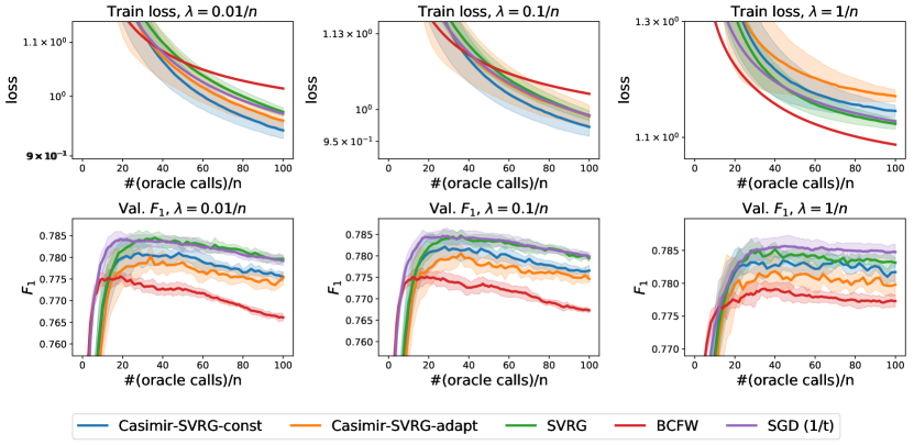
Figure 2: Comparison of convex optimization algorithms for the task of Named Entity Recognition on CoNLL 2003.

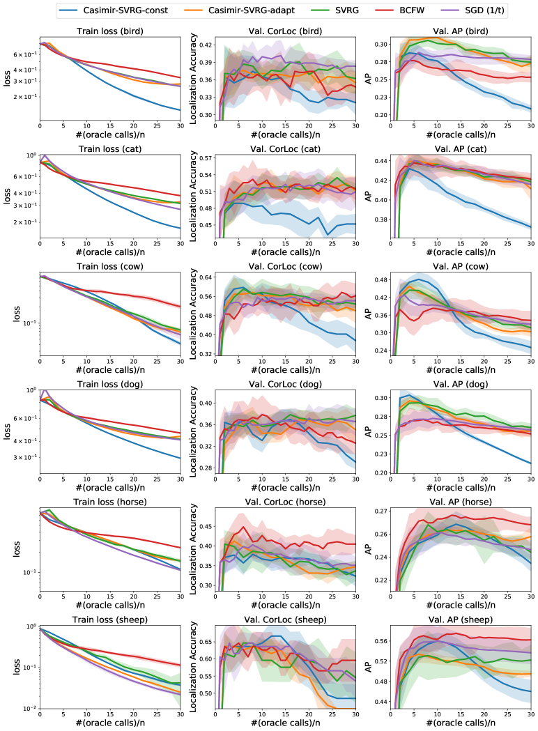
Figure 3: Comparison of convex optimization algorithms for the task of visual object localization on PASCAL VOC 2007 for $\lambda=10/n$. Plots for all other classes are in Appendix E.

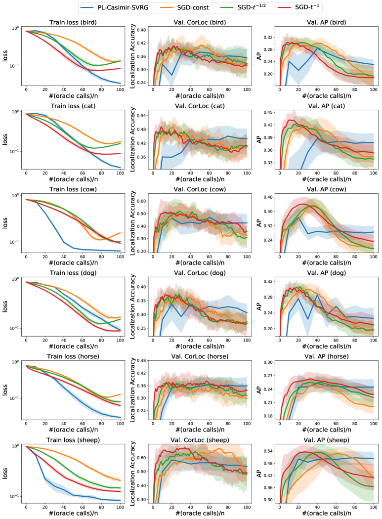
Figure 4: Comparison of non-convex optimization algorithms for the task of visual object localization on PASCAL VOC 2007 for $\lambda=1/n$. Plots for all other classes are in Appendix E.

7.4 Experimental study of different methods

Convex Optimization

For the named entity recognition task, Fig. 2 plots the performance of various methods on CoNLL 2003. On the other hand, Fig. 3 presents plots for various classes of PASCAL VOC 2007 for visual object localization.

The plots reveal that smoothing-based methods converge faster in terms of training error while achieving a competitive performance in terms of the performance metric on a held-out set. Furthermore, BCFW and SGD make twice as many actual passes as SVRG based algorithms.

Non-Convex Optimization

Fig. 4 plots the performance of various algorithms on the task of visual object localization on PASCAL VOC.

7.5 Experimental Study of Effect of Hyperparameters: Convex Optimization

We now study the effects of various hyperparameter choices.

Effect of Smoothing

Fig. 5(a) plots the effect of the level of smoothing for Casimir-SVRG-const and Casimir-SVRG-adapt. The plots reveal that, in general, small values of the smoothing parameter lead to better optimization performance for Casimir-SVRG-const. Casimir-SVRG-adapt is robust to the choice of $\mu$. Fig. 5(b) shows how the smooth optimization algorithms work when used heuristically on the non-smooth problem.

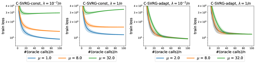
(a) Effect of level of smoothing.

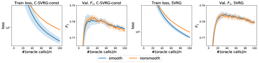
(b) Effect of smoothing: use of smooth optimization with smoothing (labeled “smooth”) versus the heuristic use of these algorithms without smoothing (labeled “non-smooth”) for $\lambda=0.01/n$.

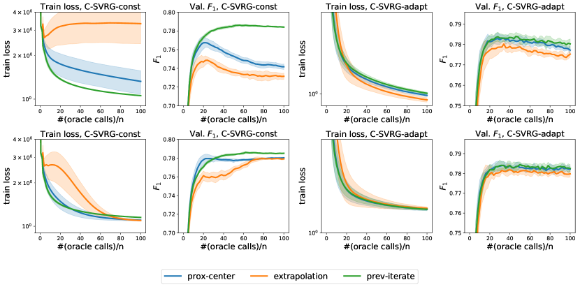
(c) Effect of warm start strategies for $\lambda=0.01/n$ (first row) and $\lambda=1/n$ (second row).

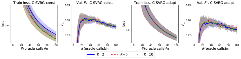
(d) Effect of $K$ in the top-$K$ oracle ($\lambda=0.01/n$).

Figure 5: Effect of hyperparameters for the task of Named Entity Recognition on CoNLL 2003. C-SVRG stands for Casimir-SVRG in these plots.

Effect of Warm Start Strategies

Fig. 5(c) plots different warm start strategies for Casimir-SVRG-const and Casimir-SVRG-adapt. We find that Casimir-SVRG-adapt is robust to the choice of the warm start strategy while Casimir-SVRG-const is not. For the latter, we observe that Extrapolation is less stable (i.e., tends to diverge more) than Prox-center, which is in turn less stable than Prev-iterate, which always works (cf. Fig. 5(c)). However, when they do work, Extrapolation and Prox-center provide greater acceleration than Prev-iterate. We use Prox-center as the default choice to trade-off between acceleration and applicability.

Effect of $K$

Fig. 5(d) illustrates the robustness of the method to choice of $K$: we observe that the results are all within one standard deviation of each other.

7.6 Experimental Study of Effect of Hyperparameters: Non-Convex Optimization

We now study the effect of various hyperparameters for the non-convex optimization algorithms. All of these comparisons have been made for $\lambda=1/n$.

Effect of Smoothing

Fig. 6(a) compares the adaptive and constant smoothing strategies. Fig. 6(b) and Fig. 6(c) compare the effect of the level of smoothing on the the both of these. As previously, the adaptive smoothing strategy is more robust to the choice of the smoothing parameter.

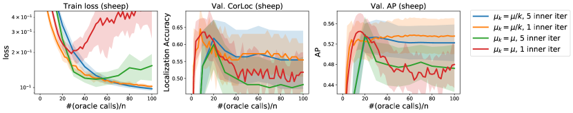
(a) Comparison of adaptive and constant smoothing strategies.

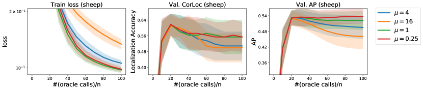
(b) Effect of $\mu$ of the adaptive smoothing strategy.

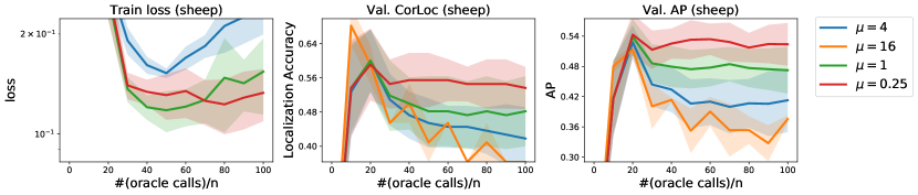
(c) Effect of $\mu$ of the constant smoothing strategy.

Figure 6: Effect of smoothing on PL-Casimir-SVRG for the task of visual object localization on PASCAL VOC 2007.

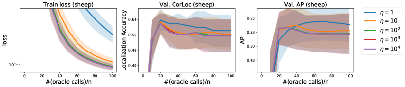
(a) Effect of the hyperparameter $\eta$.

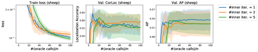
(b) Effect of the iteration budget of the inner solver.

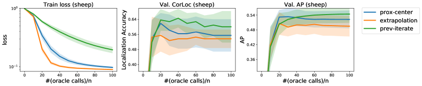
(c) Effect of the warm start strategy of the inner Casimir-SVRG-const algorithm.

Figure 7: Effect of hyperparameters on PL-Casimir-SVRG for the task of visual object localization on PASCAL VOC 2007.

Effect of Prox-Linear Learning Rate $\eta$

Fig. 7(a) shows the robustness of the proposed method to the choice of $\eta$.

Effect of Iteration Budget

Fig. 7(b) also shows the robustness of the proposed method to the choice of iteration budget of the inner solver, Casimir-SVRG-const.

Effect of Warm Start of the Inner Solver

Fig. 7(c) studies the effect of the warm start strategy used within the inner solver Casimir-SVRG-const in each inner prox-linear iteration. The results are similar to those obtained in the convex case, with Prox-center choice being the best compromise between acceleration and compatibility.

8 Future Directions

We introduced a general notion of smooth inference oracles in the context of black-box first-order optimization. This allows us to set the scene to extend the scope of fast incremental optimization algorithms to structured prediction problems owing to a careful blend of a smoothing strategy and an acceleration scheme. We illustrated the potential of our framework by proposing a new incremental optimization algorithm to train structural support vector machines both enjoying worst-case complexity bounds and demonstrating competitive performance on two real-world problems. This work paves also the way to faster incremental primal optimization algorithms for deep structured prediction models.

There are several potential venues for future work. When there is no discrete structure that admits efficient inference algorithms, it could be beneficial to not treat inference as a black-box numerical procedure (Meshi et al., 2010; Hazan and Urtasun, 2010; Hazan et al., 2016). Instance-level improved algorithms along the lines of Hazan et al. (2016) could also be interesting to explore.

Acknowledgments

This work was supported by NSF Award CCF-1740551, the Washington Research Foundation for innovation in Data-intensive Discovery, and the program “Learning in Machines and Brains” of CIFAR.

Appendix A Smoothing

We first prove an extension of Lemma 4.2 of Beck and Teboulle [2012], which proves the following statement for the special case of $\mu_{2}=0$. Recall that we defined $h_{\mu\omega}\equiv h$ when $\mu=0$.

Proposition 39.

Consider the setting of Def. 1. For $\mu_{1}\geq\mu_{2}\geq 0$, we have for every ${\bm{z}}\in\mathbb{R}^{m}$ that

$$(\mu_{1}-\mu_{2})\inf_{{\bm{u}}\in\operatorname*{dom}h^{*}}\omega({\bm{u}})\leq h_{\mu_{2}\omega}({\bm{z}})-h_{\mu_{1}\omega}({\bm{z}})\leq(\mu_{1}-\mu_{2})\sup_{{\bm{u}}\in\operatorname*{dom}h^{*}}\omega({\bm{u}})\,.$$

Proof.

We successively deduce,

$$h_{\mu_{1}\omega}({\bm{z}}) =\sup_{{\bm{u}}\in\operatorname*{dom}h^{*}}\left\{\langle{\bm{u}},{\bm{z}}\rangle-h^{*}({\bm{u}})-\mu_{1}\omega({\bm{u}})\right\}$$

$$=\sup_{{\bm{u}}\in\operatorname*{dom}h^{*}}\left\{\langle{\bm{u}},{\bm{z}}\rangle-h^{*}({\bm{u}})-\mu_{2}\omega({\bm{u}})-(\mu_{1}-\mu_{2})\omega({\bm{u}})\right\}$$

$$\geq\sup_{{\bm{u}}\in\operatorname*{dom}h^{*}}\left\{\langle{\bm{u}},{\bm{z}}\rangle-h^{*}({\bm{u}})-\mu_{2}\omega({\bm{u}})+\inf_{{\bm{u}}^{\prime}\in\operatorname*{dom}h^{*}}\left\{-(\mu_{1}-\mu_{2})\omega({\bm{u}}^{\prime})\}\right\}\right\}$$

$$=h_{\mu_{2}\omega}({\bm{z}})-(\mu_{1}-\mu_{2})\sup_{{\bm{u}}^{\prime}\in\operatorname*{dom}h^{*}}\omega({\bm{u}}^{\prime})\,,$$

since $\mu_{1}-\mu_{2}\geq 0$. The other side follows using instead that

$$-(\mu_{1}-\mu_{2})\omega({\bm{u}})\leq\sup_{{\bm{u}}^{\prime}\in\operatorname*{dom}h^{*}}\left\{-(\mu_{1}-\mu_{2})\omega({\bm{u}}^{\prime})\}\right\}\,.$$

∎

Next, we recall the following equivalent definition of a matrix norm defined in Eq. (2).

$$\|{\bm{A}}\|_{\beta,\alpha}=\sup_{{\bm{y}}\neq{\bm{0}}}\frac{\|{\bm{A}}^{\top}{\bm{y}}\|_{\beta}^{*}}{\|{\bm{y}}\|_{\alpha}}=\sup_{{\bm{x}}\neq{\bm{0}}}\frac{\|{\bm{A}}{\bm{x}}\|_{\alpha}^{*}}{\|{\bm{y}}\|_{\beta}}=\|{\bm{A}}^{\top}\|_{\alpha,\beta}\,.$$ (65)

Now, we consider the smoothness of a composition of a smooth function with an affine map.

Lemma 40.

Suppose $h:\mathbb{R}^{m}\to\mathbb{R}$ is $L$-smooth with respect to $\|\cdot\|_{\alpha}^{*}$. Then, for any ${\bm{A}}\in\mathbb{R}^{m\times d}$ and ${\bm{b}}\in\mathbb{R}^{m}$, we have that the map $\mathbb{R}^{d}\ni{\bm{w}}\mapsto h({\bm{A}}{\bm{w}}+{\bm{b}})$ is $\big{(}L\|{\bm{A}}^{\top}\|^{2}_{\alpha,\beta}\big{)}$-smooth with respect to $\|\cdot\|_{\beta}$.

Proof.

Fix ${\bm{A}}\in\mathbb{R}^{m\times d},b\in\mathbb{R}^{m}$ and define $f:\mathbb{R}^{d}\to\mathbb{R}$ as $f({\bm{w}})=h({\bm{A}}{\bm{w}}+{\bm{b}})$. By the chain rule, we have that $\nabla f({\bm{w}})={\bm{A}}^{\top}\nabla h({\bm{A}}{\bm{w}}+{\bm{b}})$. Using smoothness of $h$, we successively deduce,

$$\|\nabla f({\bm{w}}_{1})-\nabla f({\bm{w}}_{2})\|_{\beta}^{*} =\|{\bm{A}}^{\top}(\nabla h({\bm{A}}{\bm{w}}_{1}+{\bm{b}})-\nabla h({\bm{A}}{\bm{w}}_{2}+{\bm{b}}))\|_{\beta}^{*}$$

$$\stackrel{{\scriptstyle\eqref{eq:matrix_norm_defn_app}}}{{\leq}}\|{\bm{A}}^{\top}\|_{\alpha,\beta}\|\nabla h({\bm{A}}{\bm{w}}_{1}+{\bm{b}})-\nabla h({\bm{A}}{\bm{w}}_{2}+{\bm{b}})\|_{\alpha}$$

$$\leq\|{\bm{A}}^{\top}\|_{\alpha,\beta}\,L\|{\bm{A}}({\bm{w}}_{1}-{\bm{w}}_{2})\|_{\alpha}^{*}$$

$$\stackrel{{\scriptstyle\eqref{eq:matrix_norm_defn_app}}}{{\leq}}L\|{\bm{A}}^{\top}\|^{2}_{\alpha,\beta}\|{\bm{w}}_{1}-{\bm{w}}_{2}\|_{\beta}\,.$$

∎

Shown in Algo. 6 is the procedure to compute the outputs of the top-$K$ oracle from the $K$ best scoring outputs obtained, for instance, from the top-$K$ max-product algorithm.

Algorithm 6 Top-$K$ oracle from top-$K$ outputs

1:  Input: Augmented score function $\psi$, ${\bm{w}}\in\mathbb{R}^{d}$, $\mu>0$ $Y_{K}=\{{\bm{y}}_{1},\cdots,{\bm{y}}_{K}\}$ such that ${\bm{y}}_{k}=\max^{(k)}_{{\bm{y}}\in\mathcal{Y}}\psi({\bm{y}};{\bm{w}})$.

2:  Populate ${\bm{z}}\in\mathbb{R}^{K}$ so that $z_{k}=\frac{1}{\mu}\psi({\bm{y}}_{k};{\bm{w}})$.

3:  Compute ${\bm{u}}^{*}=\operatorname*{arg\,min}_{{\bm{u}}\in\Delta^{K-1}}\|{\bm{u}}-{\bm{z}}\|^{2}_{2}$ by a projection on the simplex.

4:  return  $s=\sum_{k=1}^{K}u^{*}_{k}\,\psi({\bm{y}}_{k};{\bm{w}})$ and ${\bm{v}}=\sum_{k=1}^{K}u^{*}_{k}\,\nabla_{\bm{w}}\psi({\bm{y}}_{k};{\bm{w}})$.

Appendix B Smooth Inference in Trees

A graph $\mathcal{G}$ is a tree if it is connected, directed and each node has at most one incoming edge. It has one root $r\in\mathcal{V}$ with no incoming edge. An undirected graph with no loops can be converted to a tree by fixing an arbitrary root and directing all edges way from the root. We say that $\mathcal{G}$ is a chain if it is a tree with root $p$ where all edges are of the form $(v+1,v)$. For a node $v$ in a tree $\mathcal{G}$, we denote by $\rho(v)$ and $C(v)$ respectively the parent of $v$ and the children of $v$ in the tree.

Recall first that the height of a node in a rooted tree is the number of edges on the longest directed path from the node to a leaf where each edge is directed away from the root. We first review the standard max-product algorithm for maximum a posteriori (MAP) inference [Dawid, 1992] - Algo. 7. It runs in time $\mathcal{O}(p\max_{v\in\mathcal{V}}\lvert\mathcal{Y}_{v}\rvert^{2})$ and requires space $\mathcal{O}(p\max_{v\in\mathcal{V}}\lvert\mathcal{Y}_{v}\rvert)$.

Algorithm 7 Standard max-product algorithm

1:  Input: Augmented score function $\psi(\cdot,\cdot;{\bm{w}})$ defined on tree structured graph $\mathcal{G}$ with root $r\in\mathcal{V}$.

2:  Initialize: Let $V$ be a list of nodes from $\mathcal{V}\backslash\{r\}$ arranged in increasing order of height.

3:  for $v$ in $V$ do

4:     Set $m_{v}(y_{\rho(v)})\leftarrow\max_{y_{v}\in\mathcal{Y}_{v}}\left\{\psi_{v}(y_{v})+\psi_{v,\rho(v)}(y_{v},y_{\rho(v)})+\sum_{v^{\prime}\in C(v)}m_{v^{\prime}}(y_{v})\right\}$ for each $y_{\rho(v)}\in\mathcal{Y}_{\rho(v)}$.

5:     Assign to $\delta_{v}(y_{\rho(v)})$ a maximizing assignment of $y_{v}$ from above for each $y_{\rho(v)}\in\mathcal{Y}_{\rho(v)}$.

6:  end for

7:  $\psi^{*}\leftarrow\max_{y_{r}\in\mathcal{Y}_{r}}\left\{\psi_{r}(y_{r})+\sum_{v^{\prime}\in C(r)}m_{v^{\prime}}(y_{r})\right\}$.

8:  $y_{r}^{*}\leftarrow\operatorname*{arg\,max}_{y_{r}\in\mathcal{Y}_{r}}\left\{\psi_{r}(y_{r})+\sum_{v^{\prime}\in C(r)}m_{v^{\prime}}(y_{r})\right\}$.

9:  for $v$ in $\mathrm{reverse}(V)$ do

10:     $y_{v}^{*}=\delta_{v}(y_{\rho(v)}^{*})$.

11:  end for

12:  return  $\psi^{*},{\bm{y}}^{*}=(y_{1}^{*},\cdots,y_{p}^{*})$.

Algorithm 8 Top-$K$ max-product algorithm

1:  Input: Augmented score function $\psi(\cdot,\cdot;{\bm{w}})$ defined on tree structured graph $\mathcal{G}$ with root $r\in\mathcal{V}$, and integer $K>0$.

2:  Initialize: Let $V$ be a list of nodes from $\mathcal{V}\backslash\{r\}$ arranged in increasing order of height.

3:  for $v$ in $V$ and $k=1,\cdots,K$ do

4:     if $v$ is a leaf then

5:        $m_{v}^{(k)}(y_{\rho(v)})\leftarrow\max^{(k)}_{y_{v}\in\mathcal{Y}_{v}}\left\{\psi_{v}(y_{v})+\psi_{v,\rho(v)}(y_{v},y_{\rho(v)})\right\}$ for each $y_{\rho(v)}\in\mathcal{Y}_{\rho(v)}$.

6:     else

7:        Assign for each $y_{\rho(v)}\in\mathcal{Y}_{\rho(v)}$,

$$m_{v}^{(k)}(y_{\rho(v)})\leftarrow\sideset{}{{}^{(k)}}{\max}_{\,}\left\{\begin{matrix}\psi_{v}(y_{v})+\psi_{v,\rho(v)}(y_{v},y_{\rho(v)})\\ +\sum_{v^{\prime}\in C(v)}m_{v^{\prime}}^{(l_{v^{\prime}})}(y_{v})\end{matrix}\,\middle|\,\begin{matrix}y_{v}\in\mathcal{Y}_{v}\text{ and }\\ l_{v^{\prime}}\in[K]\text{ for }v^{\prime}\in C(v)\end{matrix}\right\}\,.$$ (66)

8:        Let $\delta_{v}^{(k)}(y_{\rho(v)})$ and $\kappa_{v^{\prime}}^{(k)}(y_{\rho(v)})$ for $v^{\prime}\in C(v)$ store the maximizing assignment of $y_{v}$ and $l_{v}^{\prime}$ from above for each $y_{\rho(v)}\in\mathcal{Y}_{\rho(v)}$.

9:     end if

10:  end for

11:  For $k=1,\cdots,K$, set

$$\psi^{(k)}\leftarrow\sideset{}{{}^{(k)}}{\max}\bigg{\{}\psi_{r}(y_{r})+\sum_{v^{\prime}\in C(r)}m_{v^{\prime}}^{(l_{v^{\prime}})}(y_{r})\,\bigg{|}\,y_{r}\in\mathcal{Y}_{r}\text{ and }l_{v^{\prime}}\in[K]\text{ for }v^{\prime}\in C(r)\bigg{\}}$$

and assign maximizing assignments of $y_{r},l_{v^{\prime}}$ above respectively to $y_{r}^{(k)}$ and $l_{v^{\prime}}^{(k)}$ for $v^{\prime}\in C(r)$.

12:  for $v$ in $\mathrm{reverse}(V)$ and $k=1,\cdots,K$ do

13:     Set $y_{v}^{(k)}\leftarrow\delta_{v}^{(l^{(k)}_{v})}\big{(}y_{\rho(v)}^{(k)}\big{)}$.

14:     Set $l_{v^{\prime}}^{(k)}=\kappa_{v^{\prime}}^{(l^{(k)}_{v})}\big{(}y_{\rho(v)}^{(k)}\big{)}$ for all $v^{\prime}\in C(v)$.

15:  end for

16:  return  $\left\{\psi^{(k)},{\bm{y}}^{(k)}:=(y_{1}^{(k)},\cdots,y_{p}^{(k)})\right\}_{k=1}^{K}$.

B.1 Proof of Correctness of Top-$K$ Max-Product

We now consider the top-$K$ max-product algorithm, shown in full generality in Algo. 8. The following proposition proves its correctness.

Proposition 41.

Consider as inputs to Algo. 8 an augmented score function $\psi(\cdot,\cdot;{\bm{w}})$ defined on tree structured graph $\mathcal{G}$, and an integer $K>0$. Then, the outputs of Algo. 8 satisfy $\psi^{(k)}=\psi({\bm{y}}^{(k)})=\sideset{}{{}^{(k)}}{\max}_{{\bm{y}}\in\mathcal{Y}}\psi({\bm{y}})$. Moreover, Algo. 8 runs in time $\mathcal{O}(pK\log K\max_{v\in\mathcal{V}}\lvert\mathcal{Y}_{v}\rvert^{2})$ and uses space $\mathcal{O}(pK\max_{v\in\mathcal{V}}\lvert\mathcal{Y}_{v}\rvert)$.

Proof.

For a node $v\in\mathcal{V}$, let $\tau(v)$ denote the sub-tree of $\mathcal{G}$ rooted at $v$. Let ${\bm{y}}_{\tau(v)}$ denote $\big{(}y_{v^{\prime}}\text{ for }v^{\prime}\in\tau(v)\big{)}$. Define $\psi_{\tau(v)}$ as follows: if $v$ is a leaf, ${\bm{y}}_{\tau(v)}=(y_{v})$ and $\psi_{\tau(v)}({\bm{y}}_{\tau(v)}):=\psi_{v}(y_{v})$. For a non-leaf $v$, define recursively

$$\psi_{\tau(v)}({\bm{y}}_{\tau(v)}):=\psi_{v}(y_{v})+\sum_{v^{\prime}\in C(v)}\left[\psi_{v,v^{\prime}}(y_{v},y_{v^{\prime}})+\psi_{\tau(v^{\prime})}({\bm{y}}_{\tau(v^{\prime})})\right]\,.$$ (67)

We will need some identities about choosing the $k$th largest element from a finite collection. For finite sets $S_{1},\cdots,S_{n}$ and functions $f_{j}:S_{j}\to\mathbb{R}$, $h:S_{1}\times S_{2}\to\mathbb{R}$, we have,

$$\sideset{}{{}^{(k)}}{\max}_{u_{1}\in S_{1},\cdots,u_{n}\in S_{n}}\left\{\sum_{j=1}^{n}f_{j}(u_{j})\right\}=\quad\sideset{}{{}^{(k)}}{\max}_{l_{1},\cdots,l_{n}\in[k]}\left\{\sum_{j=1}^{n}\sideset{}{{}^{(l_{j})}}{\max}_{u_{j}\in S_{j}}f_{j}(u_{j})\right\}\,,$$ (68)

$$\sideset{}{{}^{(k)}}{\max}_{u_{1}\in S_{1},u_{2}\in S_{2}}\{f_{1}(u_{1})+h(u_{1},u_{2})\}=\quad\sideset{}{{}^{(k)}}{\max}_{u_{1}\in S_{1},l\in[k]}\left\{f_{1}(u_{1})+\sideset{}{{}^{(l)}}{\max}_{u_{2}\in S_{2}}h(u_{1},u_{2})\right\}\,.$$ (69)

The identities above state that for a sum to take its $k$th largest value, each component of the sum must take one of its $k$ largest values. Indeed, if one of the components of the sum took its $l$th largest value for $l>k$, replacing it with any of the $k$ largest values cannot decrease the value of the sum. Eq. (69) is a generalized version of Bellman’s principle of optimality (see Bellman [1957, Chap. III.3.] or Bertsekas [1995, Vol. I, Chap. 1]).

For the rest of the proof, ${\bm{y}}_{\tau(v)}\backslash y_{v}$ is used as shorthand for $\{y_{v^{\prime}}\,|\,v^{\prime}\in\tau(v)\backslash\{v\}\}$. Moreover, $\max_{{\bm{y}}_{\tau(v)}}$ represents maximization over ${\bm{y}}_{\tau(v)}\in\bigtimes_{v^{\prime}\in\tau(v)}\mathcal{Y}_{v^{\prime}}$. Likewise for $\max_{{\bm{y}}_{\tau(v)}\backslash y_{v}}$. Now, we shall show by induction that for all $v\in\mathcal{V}$, $y_{v}\in\mathcal{Y}_{v}$ and $k=1,\cdots,K$,

$$\sideset{}{{}^{(k)}}{\max}_{{\bm{y}}_{\tau(v)}\backslash y_{v}}\psi_{\tau(v)}({\bm{y}}_{\tau(v)})=\psi_{v}(y_{v})+\sideset{}{{}^{(k)}}{\max}\bigg{\{}\sum_{v^{\prime}\in C(v)}m_{v^{\prime}}^{(l_{v^{\prime}})}(y_{v^{\prime}})\bigg{|}l_{v^{\prime}}\in[K]\text{ for }v^{\prime}\in C(v)\bigg{\}}\,.$$ (70)

The induction is based on the height of a node. The statement is clearly true for a leaf $v$ since $C(v)=\varnothing$. Suppose (70) holds for all nodes of height $\leq h$. For a node $v$ of height $h+1$, we observe that $\tau(v)\backslash v$ can be partitioned into $\{\tau(v^{\prime})\text{ for }v^{\prime}\in C(v)\}$ to get,

$$\sideset{}{{}^{(k)}}{\max}_{{\bm{y}}_{\tau(v)}\backslash y_{v}}\psi_{\tau(v)}({\bm{y}}_{\tau(v)})-\psi_{v}(y_{v})\stackrel{{\scriptstyle\eqref{eq:dp:topk_proof:phi_subtree}}}{{=}}\sideset{}{{}^{(k)}}{\max}_{{\bm{y}}_{\tau(v)}\backslash y_{v}}\bigg{\{}\sum_{v^{\prime}\in C(v)}\psi_{v,v^{\prime}}(y_{v},y_{v^{\prime}})+\psi_{\tau(v^{\prime})}({\bm{y}}_{\tau(v^{\prime})})\bigg{\}}$$

$$\stackrel{{\scriptstyle\eqref{eq:dp:topk_proof:bellman1}}}{{=}}\sideset{}{{}^{(k)}}{\max}\bigg{\{}\sum_{v^{\prime}\in C(v)}\underbrace{\sideset{}{{}^{(l_{v^{\prime}})}}{\max}_{{\bm{y}}_{\tau(v^{\prime})}}\{\psi_{v,v^{\prime}}(y_{v},y_{v^{\prime}})+\psi_{\tau(v^{\prime})}({\bm{y}}_{\tau(v^{\prime})})\}}_{=:\mathcal{T}_{v^{\prime}}(y_{v})}\,\bigg{|}\,l_{v^{\prime}}\in[K]\text{ for }v^{\prime}\in C(v)\bigg{\}}\,.$$ (71)

Let us analyze the term in the underbrace, $\mathcal{T}_{v^{\prime}}(y_{v})$. We successively deduce, with the argument $l$ in the maximization below taking values in $\{1,\cdots,K\}$,

$$\mathcal{T}_{v^{\prime}}(y_{v}) \stackrel{{\scriptstyle\eqref{eq:dp:topk_proof:bellman2}}}{{=}}\sideset{}{{}^{(l_{v^{\prime}})}}{\max}_{y_{v^{\prime}},l}\bigg{\{}\psi_{v,v^{\prime}}(y_{v},y_{v^{\prime}})+\sideset{}{{}^{(l)}}{\max}_{{\bm{y}}_{\tau(v^{\prime})}\backslash y_{v^{\prime}}}\psi_{\tau(v^{\prime})}({\bm{y}}_{\tau(v^{\prime})})\bigg{\}}$$

$$\stackrel{{\scriptstyle\eqref{eq:dp:topk_proof:ind_hyp}}}{{=}}\sideset{}{{}^{(l_{v^{\prime}})}}{\max}_{y_{v^{\prime}},l}\bigg{\{}\begin{matrix}\psi_{v^{\prime}}(y_{v^{\prime}})+\psi_{v,v^{\prime}}(y_{v},y_{v^{\prime}})+\\ \sideset{}{{}^{(l)}}{\max}\big{\{}\sum_{v^{\prime\prime}\in C(v^{\prime})}m_{v^{\prime\prime}}^{(l_{v^{\prime\prime}})}(y_{v^{\prime}})\,|\,l_{v^{\prime\prime}}\in[K]\text{ for }v^{\prime\prime}\in C(v^{\prime})\big{\}}\end{matrix}\bigg{\}}$$

$$\stackrel{{\scriptstyle\eqref{eq:dp:topk_proof:bellman2}}}{{=}}\sideset{}{{}^{(l_{v^{\prime}})}}{\max}\bigg{\{}\begin{matrix}\psi_{v^{\prime}}(y_{v^{\prime}})+\psi_{v^{\prime},v}(y_{v^{\prime}},y_{v})\\ +\sum_{v^{\prime\prime}\in C(v^{\prime})}m^{(l_{v^{\prime\prime}})}_{v^{\prime\prime}}(y_{v^{\prime}})\end{matrix}\,\bigg{|}\,\begin{matrix}y_{v^{\prime}}\in\mathcal{Y}_{v^{\prime}}\text{ and }\\ l_{v^{\prime\prime}}\in[K]\text{ for }v^{\prime\prime}\in C(v)\end{matrix}\bigg{\}}$$

$$\stackrel{{\scriptstyle\eqref{eq:dp:topk:algo:update}}}{{=}}m^{(l_{v^{\prime}})}_{v^{\prime}}(y_{v})\,.$$

Here, the penultimate step followed from applying in reverse the identity (69) with $u_{1},u_{2}$ being by $y_{v^{\prime}},\{l_{v^{\prime\prime}}\text{ for }v^{\prime\prime}\in C(v^{\prime})\}$ respectively, and $f_{1}$ and $h$ respectively being $\psi_{v^{\prime}}(y_{v^{\prime}})+\psi_{v^{\prime},v}(y_{v^{\prime}},y_{v})$ and $\sum_{v^{\prime\prime}}m^{(l_{v^{\prime\prime}})}_{v^{\prime\prime}}(y_{v^{\prime}})$. Plugging this into (71) completes the induction argument. To complete the proof, we repeat the same argument over the root as follows. We note that $\tau(r)$ is the entire tree $\mathcal{G}$. Therefore, ${\bm{y}}_{\tau(r)}={\bm{y}}$ and $\psi_{\tau(r)}=\psi$. We now apply the identity (69) with $u_{1}$ and $u_{2}$ being $y_{r}$ and ${\bm{y}}_{\tau(r)\backslash r}$ respectively and $f_{1}\equiv 0$ to get

$$\sideset{}{{}^{(k)}}{\max}_{{\bm{y}}\in\mathcal{Y}}\psi({\bm{y}}) \stackrel{{\scriptstyle\eqref{eq:dp:topk_proof:bellman2}}}{{=}}\sideset{}{{}^{(k)}}{\max}_{y_{r},l}\left\{\sideset{}{{}^{(l)}}{\max}_{{\bm{y}}\backslash y_{r}}\psi({\bm{y}})\right\}=\sideset{}{{}^{(k)}}{\max}_{y_{r},l}\left\{\sideset{}{{}^{(l)}}{\max}_{{\bm{y}}_{\tau(r)}\backslash y_{r}}\psi_{\tau(r)}({\bm{y}}_{\tau(r)})\right\}$$

$$\stackrel{{\scriptstyle\eqref{eq:dp:topk_proof:ind_hyp}}}{{=}}\sideset{}{{}^{(k)}}{\max}_{y_{r},l}\bigg{\{}\begin{matrix}\psi_{r}(y_{r})+\sideset{}{{}^{(l)}}{\max}\big{\{}\sum_{v\in C(r)}m_{v}^{(l_{v})}(y_{r})\,|\,l_{v}\in[K]\text{ for }v\in C(r)\big{\}}\end{matrix}\bigg{\}}$$

$$\stackrel{{\scriptstyle\eqref{eq:dp:topk_proof:bellman2}}}{{=}}\sideset{}{{}^{(k)}}{\max}\bigg{\{}\begin{matrix}\psi_{r}(y_{r})+\\ \sum_{v\in C(r)}m^{(l_{v})}_{v}(y_{r})\end{matrix}\,\bigg{|}\,\begin{matrix}y_{r}\in\mathcal{Y}_{r}\text{ and }\\ l_{v}\in[K]\text{ for }v\in C(r)\end{matrix}\bigg{\}}$$

$$\,=\psi^{(k)}\,,$$

where the last equality follows from Line 11 of Algo. 8.

The algorithm requires storage of $m_{v}^{(k)}$, an array of size $\max_{v\in\mathcal{V}}\lvert\mathcal{Y}_{v}\rvert$ for each $k=1,\cdots,K$, and $v\in\mathcal{V}$. The backpointers $\delta,\kappa$ are of the same size. This adds up to a total storage of $\mathcal{O}(pK\max_{v}\lvert\mathcal{Y}_{v}\rvert)$. To bound the running time, consider Line 7 of Algo. 8. For a fixed $v^{\prime}\in C(v)$, the computation

$$\sideset{}{{}^{(k)}}{\max}_{y_{v},l_{v^{\prime}}}\left\{\psi_{v}(y_{v})+\psi_{v,\rho(v)}(y_{v},y_{\rho(v)})+m_{v^{\prime}}^{(l_{v^{\prime}})}(y_{v})\right\}$$

for $k=1,\cdots,K$ takes time $\mathcal{O}(K\log K\max_{v}\lvert\mathcal{Y}_{v}\rvert)$. This operation is repeated for each $y_{v}\in\mathcal{Y}_{v}$ and once for every $(v,v^{\prime})\in\mathcal{E}$. Since $\lvert\mathcal{E}\rvert=p-1$, the total running time is $\mathcal{O}(pK\log K\max_{v}\lvert\mathcal{Y}_{v}\rvert^{2})$. ∎

B.2 Proof of Correctness of Entropy Smoothing of Max-Product

Next, we consider entropy smoothing.

Proposition 42.

Given an augmented score function $\psi(\cdot,\cdot;{\bm{w}})$ defined on tree structured graph $\mathcal{G}$ and $\mu>0$ as input, Algo. 3 correctly computes $f_{-\mu H}({\bm{w}})$ and $\nabla f_{-\mu H}({\bm{w}})$. Furthermore, Algo. 3 runs in time $\mathcal{O}(p\max_{v\in\mathcal{V}}\lvert\mathcal{Y}_{v}\rvert^{2})$ and requires space $\mathcal{O}(p\max_{v\in\mathcal{V}}\lvert\mathcal{Y}_{v}\rvert)$.

Proof.

The correctness of the function value $f_{-\mu H}$ follows from the bijection $f_{-\mu H}({\bm{w}})=\mu\,A_{\psi/\mu}({\bm{w}})$ (cf. Prop. 9), where Thm. 43 shows correctness of $A_{\psi/\mu}$. To show the correctness of the gradient, define the probability distribution $P_{\psi,\mu}$ as the probability distribution from Lemma 7(ii) and $P_{\psi,\mu,v},P_{\psi,\mu,v,v^{\prime}}$ as its node and edge marginal probabilities respectively as

$$P_{\psi,\mu}({\bm{y}};{\bm{w}}) =\frac{\exp\left(\tfrac{1}{\mu}\psi({\bm{y}};{\bm{w}})\right)}{\sum_{{\bm{y}}^{\prime}\in\mathcal{Y}}\exp\left(\tfrac{1}{\mu}\psi({\bm{y}}^{\prime};{\bm{w}})\right)}\,,$$

$$P_{\psi,\mu,v}(\overline{y}_{v};{\bm{w}}) =\sum_{\begin{subarray}{c}{\bm{y}}\in\mathcal{Y}\,:\\ y_{v}=\overline{y}_{v}\end{subarray}}P_{\psi,\mu}({\bm{y}};{\bm{w}})\quad\text{for }\overline{y}_{v}\in\mathcal{Y}_{v},v\in\mathcal{V}\,,\text{ and, }$$

$$P_{\psi,\mu,v,v^{\prime}}(\overline{y}_{v},\overline{y}_{v^{\prime}};{\bm{w}}) =\sum_{\begin{subarray}{c}{\bm{y}}\in\mathcal{Y}:\\ y_{v}=\overline{y}_{v},\\ y_{v^{\prime}}=\overline{y}_{v^{\prime}}\end{subarray}}P_{\psi,\mu}({\bm{y}};{\bm{w}})\quad\text{for }\overline{y}_{v}\in\mathcal{Y}_{v},\overline{y}_{v^{\prime}}\in\mathcal{Y}_{v^{\prime}},(v,v^{\prime})\in\mathcal{E}\,.$$

Thm. 43 again shows that Algo. 9 correctly produces marginals $P_{\psi,\mu,v}$ and $P_{\psi,\mu,v,v^{\prime}}$. We now start with Lemma 7(ii) and invoke (17) to get

$$\nabla f_{-\mu H}({\bm{w}})= \sum_{{\bm{y}}\in\mathcal{Y}}P_{\psi,\mu}({\bm{y}};{\bm{w}})\nabla\psi({\bm{y}};{\bm{w}})$$

$${=} \sum_{{\bm{y}}\in\mathcal{Y}}P_{\psi,\mu}({\bm{y}};{\bm{w}})\left(\sum_{v\in\mathcal{V}}\nabla\psi_{v}(y_{v};{\bm{w}})+\sum_{(v,v^{\prime})\in\mathcal{E}}\nabla\psi_{v,v^{\prime}}(y_{v},y_{v^{\prime}};{\bm{w}})\right)\,,$$

$$= \sum_{v\in\mathcal{V}}\sum_{{\bm{y}}\in\mathcal{Y}}P_{\psi,\mu}({\bm{y}};{\bm{w}})\nabla\psi_{v}(y_{v};{\bm{w}})+\sum_{(v,v^{\prime})\in\mathcal{E}}\sum_{{\bm{y}}\in\mathcal{Y}}P_{\psi,\mu}({\bm{y}};{\bm{w}})\nabla\psi_{v,v^{\prime}}(y_{v},y_{v^{\prime}};{\bm{w}})$$

$$= \sum_{v\in\mathcal{V}}\sum_{\overline{y}_{v}\in\mathcal{Y}_{v}}\sum_{{\bm{y}}\in\mathcal{Y}\,:\,y_{v}=\overline{y}_{v}}P_{\psi,\mu}({\bm{y}};{\bm{w}})\nabla\psi_{v}(\overline{y}_{v};{\bm{w}})$$

$$\qquad+\sum_{(v,v^{\prime})\in\mathcal{E}}\sum_{\overline{y}_{v}\in\mathcal{Y}_{v}}\sum_{\overline{y}_{v^{\prime}}\in\mathcal{Y}_{v^{\prime}}}\sum_{{\bm{y}}\in\mathcal{Y}\,:\,\begin{subarray}{c}y_{v}=\overline{y}_{v}\\ y_{v^{\prime}}=\overline{y}_{v^{\prime}}\end{subarray}}P_{\psi,\mu}({\bm{y}};{\bm{w}})\nabla\psi_{v,v^{\prime}}(\overline{y}_{v},\overline{y}_{v^{\prime}};{\bm{w}})$$

$$= \sum_{v\in\mathcal{V}}\sum_{\overline{y}_{v}\in\mathcal{Y}_{v}}P_{\psi,\mu,v}(\overline{y}_{v};{\bm{w}})\nabla\psi_{v}(\overline{y}_{v};{\bm{w}})$$

$$\qquad+\sum_{(v,v^{\prime})\in\mathcal{E}}\sum_{\overline{y}_{v}\in\mathcal{Y}_{v}}\sum_{\overline{y}_{v^{\prime}}\in\mathcal{Y}_{v^{\prime}}}P_{\psi,\mu,v,v^{\prime}}(\overline{y}_{v},\overline{y}_{v^{\prime}};{\bm{w}})\nabla\psi_{v,v^{\prime}}(\overline{y}_{v},\overline{y}_{v^{\prime}};{\bm{w}})\,.$$

Here, the penultimate equality followed from breaking the sum over ${\bm{y}}\in\mathcal{Y}$ into an outer sum that sums over every $\overline{y}_{v}\in\mathcal{Y}_{v}$ and an inner sum over ${\bm{y}}\in\mathcal{Y}:y_{v}=\overline{y}_{v}$, and likewise for the edges. The last equality above followed from the definitions of the marginals. Therefore, Line 3 of Algo. 3 correctly computes the gradient. The storage complexity of the algorithm is $\mathcal{O}(p\max_{v}\lvert\mathcal{Y}_{v}\rvert)$ provided that the edge marginals $P_{\psi,\mu,v,v^{\prime}}$ are computed on the fly as needed. The time overhead of Algo. 3 after Algo. 9 is $\mathcal{O}(p\max_{v}\lvert\mathcal{Y}_{v}\rvert^{2})$, by noting that each edge marginal can be computed in constant time (Remark 44). ∎

Algorithm 9 Sum-product algorithm

1:  Procedure: SumProduct

2:  Input: Augmented score function $\psi$ defined on tree structured graph $\mathcal{G}$ with root $r\in\mathcal{V}$.

3:  Notation: Let $N(v)=C(v)\cup\{\rho(v)\}$ denote all the neighbors of $v\in\mathcal{V}$ if the orientation of the edges were ignored.

4:  Initialize: Let $V$ be a list of nodes from $\mathcal{V}$ arranged in increasing order of height.

5:  for $v$ in $V\backslash\{r\}$ do

6:     Set for each $y_{\rho(v)}\in\mathcal{Y}_{\rho(v)}$:

$$m_{v\to\rho(v)}(y_{\rho(v)})\leftarrow\sum_{y_{v}\in\mathcal{Y}_{v}}\left[\exp\left(\psi_{v}(y_{v})+\psi_{v,\rho(v)}(y_{v},y_{\rho(v)})\right)\prod_{v^{\prime}\in C(v)}m_{v^{\prime}\to v}(y_{v})\right]\,.$$

7:  end for

8:  $A\leftarrow\log\sum_{y_{r}\in\mathcal{Y}_{r}}\left[\exp\left(\psi_{r}(y_{r})\right)\prod_{v^{\prime}\in C(r)}m_{v^{\prime}\to r}(y_{r})\right]$.

9:  for $v$ in $\mathrm{reverse}(V)$ do

10:     for $v^{\prime}\in C(v)$ do

11:        Set for each $y_{v^{\prime}}\in\mathcal{Y}_{v^{\prime}}$:

$$m_{v\to v^{\prime}}(y_{v^{\prime}})=\sum_{y_{v}\in\mathcal{Y}_{v}}\left[\exp\left(\psi_{v}(y_{v})+\psi_{v^{\prime},v}(y_{v^{\prime}},y_{v})\right)\prod_{v^{\prime\prime}\in N(v)\backslash\{v^{\prime}\}}m_{v^{\prime\prime}\to v}(y_{v})\right]\,.$$

12:     end for

13:  end for

14:  for  $v$ in $\mathcal{V}$ do

15:     Set $P_{v}(y_{v})\leftarrow\exp\left(\psi_{v}(y_{v})-A\right)\prod_{v^{\prime\prime}\in N(v)}m_{v^{\prime\prime}\to v}(y_{v})$ for every $y_{v}\in\mathcal{Y}_{v}$.

16:  end for

17:  for $(v,v^{\prime})$ in $\mathcal{E}$ do

18:     For every pair $(y_{v},y_{v^{\prime}})\in\mathcal{Y}_{v}\times\mathcal{Y}_{v^{\prime}}$, set

$$P_{v,v^{\prime}}(y_{v},y_{v^{\prime}})\leftarrow \exp\left(\psi_{v}(y_{v})+\psi_{v^{\prime}}(y_{v^{\prime}})+\psi_{v,v^{\prime}}(y_{v},y_{v^{\prime}})-A\right)$$

$$\prod_{v^{\prime\prime}\in N(v)\backslash\{v^{\prime}\}}m_{v^{\prime\prime}\to v}(y_{v})\prod_{v^{\prime\prime}\in N(v^{\prime})\backslash\{v\}}m_{v^{\prime\prime}\to v^{\prime}}(y_{v^{\prime}})\,.$$

19:  end for

20:  return  $A,\{P_{v}\text{ for }v\in\mathcal{V}\},\{P_{v,v^{\prime}}\text{ for }(v,v^{\prime})\in\mathcal{E}\}$.

Given below is the guarantee of the sum-product algorithm (Algo. 9). See, for instance, Koller and Friedman [2009, Ch. 10] for a proof.

Theorem 43.

Consider an augmented score function $\psi$ defined over a tree structured graphical model $\mathcal{G}$. Then, the output of Algo. 9 satisfies

$$A =\log\sum_{{\bm{y}}\in\mathcal{Y}}\exp(\psi({\bm{y}}))\,,$$

$$P_{v}(\overline{y}_{v}) =\sum_{{\bm{y}}\in\mathcal{Y}\,:\,y_{v}=\overline{y}_{v}}\exp(\psi({\bm{y}})-A)\,\quad\text{for all $\overline{y}_{v}\in\mathcal{Y}_{v},v\in\mathcal{V}$, and, }\,$$

$$P_{v,v^{\prime}}(\overline{y}_{v},\overline{y}_{v^{\prime}}) =\sum_{{\bm{y}}\in\mathcal{Y}\,:\,\begin{subarray}{c}y_{v}=\overline{y}_{v},\\ y_{v^{\prime}}=\overline{y}_{v^{\prime}}\end{subarray}}\exp(\psi({\bm{y}})-A)\,\quad\text{for all $\overline{y}_{v}\in\mathcal{Y}_{v},\overline{y}_{v^{\prime}}\in\mathcal{Y}_{v^{\prime}},(v,v^{\prime})\in\mathcal{E}$.}$$

Furthermore, Algo. 9 runs in time $\mathcal{O}(p\max_{v\in\mathcal{V}}\lvert\mathcal{Y}_{v}\rvert^{2})$ and requires an intermediate storage of $\mathcal{O}(p\max_{v\in\mathcal{V}}\lvert\mathcal{Y}_{v}\rvert)$.

Remark 44.

Line 18 of Algo. 9 can be implemented in constant time by reusing the node marginals $P_{v}$ and messages $m_{v\to v^{\prime}},m_{v^{\prime}\to v}$ as

$$P_{v,v^{\prime}}(y_{v},y_{v^{\prime}})=\frac{P_{v}(y_{v})P_{v^{\prime}}(y_{v^{\prime}})\exp(\psi_{v,v^{\prime}}(y_{v},y_{v^{\prime}})+A)}{m_{v^{\prime}\to v}(y_{v})m_{v\to v^{\prime}}(y_{v^{\prime}})}\,.$$

Appendix C Inference Oracles in Loopy Graphs

This section presents the missing details and recalls from literature the relevant algorithms and results required in Sec. 4.2. First, we review the BMMF algorithm of Yanover and Weiss [2004], followed by graph cut inference and graph matching inference.

We now recall and prove the correctness of the decoding scheme (21) for completeness. The result is due to Pearl [1988], Dawid [1992].

Theorem 45.

Consider an unambiguous augmented score function $\psi$ , that is, $\psi({\bm{y}}^{\prime};{\bm{w}})\neq\psi({\bm{y}}^{\prime\prime};{\bm{w}})$ for all distinct ${\bm{y}}^{\prime},{\bm{y}}^{\prime\prime}\in\mathcal{Y}$. Then, the result $\widehat{\bm{y}}$ of the decoding $\widehat{y}_{v}=\operatorname*{arg\,max}_{j\in\mathcal{Y}_{v}}\psi_{v;j}$ satisfies $\widehat{\bm{y}}=\operatorname*{arg\,max}_{{\bm{y}}\in\mathcal{Y}}\psi({\bm{y}})$.

Proof.

Suppose for the sake of contradiction that $\widehat{\bm{y}}\neq{\bm{y}}^{*}:=\operatorname*{arg\,max}_{{\bm{y}}\in\mathcal{Y}}\psi({\bm{y}})$. Let $v\in\mathcal{V}$ be such that $y_{v}=j$ and $y^{*}_{v}=j^{\prime}$ where $j\neq j^{\prime}$. By the fact that ${\bm{y}}^{*}$ has the highest augmented score and unambiguity, we get that

$$\max_{{\bm{y}}\in\mathcal{Y},{\bm{y}}_{v}=j^{\prime}}\psi({\bm{y}})=\psi({\bm{y}}^{*})>\psi(\widehat{\bm{y}})=\max_{{\bm{y}}\in\mathcal{Y},{\bm{y}}_{v}=j}\psi({\bm{y}})\,,$$

which contradicts the definition of $\widehat{y}_{v}$. ∎

C.1 Review of Best Max-Marginal First

If one has access to an algorithm $\mathcal{M}$ that can compute max-marginals, the top-$K$ oracle is easily implemented via the Best Max Marginal First (BMMF) algorithm of Yanover and Weiss [2004], which is recalled in Algo. 10. This algorithm requires computations of two sets of max-marginals per iteration, where a set of max-marginals refers to max-marginals for all variables $y_{v}$ in ${\bm{y}}$.

Details

The algorithm runs by maintaining a partitioning of the search space $\mathcal{Y}$ and a table $\varphi^{(k)}(v,j)$ that stores the best score in partition $k$ (defined by constraints $\mathcal{C}^{(k)}$) subject to the additional constraint that $y_{v}=j$. In iteration $k$, the algorithm looks at the $k-1$ existing partitions and picks the best partition $s_{k}$ (Line 9). This partition is further divided into two parts: the max-marginals in the promising partition (corresponding to $y_{v_{k}}=j_{k}$) are computed (Line 11) and decoded (Line 12) to yield $k$th best scoring ${\bm{y}}^{(k)}$. The scores of the less promising partition are updated via a second round of max-marginal computations (Line 14).

Algorithm 10 Best Max Marginal First (BMMF)

1:  Input: Augmented score function $\psi$, parameters ${\bm{w}}$, non-negative integer $K$, algorithm $\mathcal{M}$ to compute max-marginals of $\psi$.

2:  Initialization: $\mathcal{C}^{(1)}=\varnothing$ and $\mathcal{U}^{(2)}=\varnothing$.

3:  for $v\in[p]$ do

4:     For $j\in\mathcal{Y}_{v}$, set $\varphi^{(1)}(v;j)=\max\{\psi({\bm{y}};{\bm{w}})\,|\,{\bm{y}}\in\mathcal{Y}\text{ s.t. }y_{v}=j\}$ using $\mathcal{M}$.

5:     Set $y^{(1)}_{v}=\operatorname*{arg\,max}_{j\in\mathcal{Y}_{v}}\varphi^{(1)}(v,j)$.

6:  end for

7:  for $k=2,\cdots,K$ do

8:     Define search space $\mathcal{S}^{(k)}=\left\{(v,j,s)\in[p]\times\mathcal{Y}_{v}\times[k-1]\,\big{|}\,y^{(s)}_{v}\neq j,\text{ and }(v,j,s)\notin\mathcal{U}^{(t)}\right\}$.

9:     Find indices $(v_{k},j_{k},s_{k})=\operatorname*{arg\,max}_{(v,j,s)\in\mathcal{S}^{(k)}}\varphi^{(s)}(v,j)$ and set constraints $\mathcal{C}^{(k)}=\mathcal{C}^{(s_{k})}\cup\{y_{v_{k}}=j_{k}\}$.

10:     for $v\in[p]$ do

11:        For each $j\in\mathcal{Y}_{v}$, use $\mathcal{M}$ to set $\varphi^{(k)}(v,j)=\max\left\{\psi({\bm{y}};{\bm{w}})\,|\,{\bm{y}}\in\mathcal{Y}\text{ s.t. constraints }\mathcal{C}^{(k)}\text{ hold and }y_{v}=j\right\}$.

12:        Set $y^{(k)}_{v}=\operatorname*{arg\,max}_{j\in\mathcal{Y}_{v}}\varphi^{(k)}(v,j)$.

13:     end for

14:     Update $\mathcal{U}^{(k+1)}=\mathcal{U}^{(k)}\cup\left\{(v_{k},j_{k},s_{k})\right\}$ and $\mathcal{C}^{(s_{k})}=\mathcal{C}^{(s_{k})}\cup\{y_{v_{k}}\neq j_{k}\}$ and the max-marginal table $\varphi^{(s_{k})}(v,j)=\max_{{\bm{y}}\in\mathcal{Y},\mathcal{C}^{(s_{k})},y_{v}=j}\psi({\bm{y}};{\bm{w}})$ using $\mathcal{M}$.

15:  end for

16:  return  $\left\{\left(\psi({\bm{y}}^{(k)};{\bm{w}}),{\bm{y}}^{(k)}\right)\right\}_{k=1}^{K}$.

Guarantee

The following theorem shows that Algo. 10 provably implements the top-$K$ oracle as long as the max-marginals can be computed exactly under the assumption of unambiguity. With approximate max-marginals however, Algo. 10 comes with no guarantees.

Theorem 46 (Yanover and Weiss [2004]).

Suppose the score function $\psi$ is unambiguous, that is, $\psi({\bm{y}}^{\prime};{\bm{w}})\neq\psi({\bm{y}}^{\prime\prime};{\bm{w}})$ for all distinct ${\bm{y}}^{\prime},{\bm{y}}^{\prime\prime}\in\mathcal{Y}$. Given an algorithm $\mathcal{M}$ that can compute the max-marginals of $\psi$ exactly, Algo. 10 makes at most $2K$ calls to $\mathcal{M}$ and its output satisfies $\psi({\bm{y}}_{k};{\bm{w}})=\max^{(k)}_{{\bm{y}}\in\mathcal{Y}}\psi({\bm{y}};{\bm{w}})$. Thus, the BMMF algorithm followed by a projection onto the simplex (Algo. 6 in Appendix A) is a correct implementation of the top-$K$ oracle. It makes $2K$ calls to $\mathcal{M}$.

Constrained Max-Marginals

The algorithm requires computation of max-marginals subject to constraints of the form $y_{v}\in Y_{v}$ for some set $Y_{v}\subseteq\mathcal{Y}_{v}$. This is accomplished by redefining for a constraint $y_{v}\in Y_{v}$:

$$\overline{\psi}({\bm{y}})=\begin{cases}\psi({\bm{y}}),\,\text{ if }y_{v}\in Y_{v}\\ -\infty,\,\text{ otherwise}\end{cases}\,.$$

C.2 Max-Marginals Using Graph Cuts

Algorithm 11 Max-marginal computation via Graph Cuts

1:  Input: Augmented score function $\psi(\cdot,\cdot;{\bm{w}})$ with $\mathcal{Y}=\{0,1\}^{p}$, constraints $\mathcal{C}$ of the form $y_{v}=b$ for $b\in\{0,1\}$.

2:  Using artificial source $s$ and sink $t$, set $V^{\prime}=\mathcal{V}\cup\{s,t\}$ and $E^{\prime}=\varnothing$.

3:  for $v\in[p]$ do

4:     Add to $E^{\prime}$ the (edge, cost) pairs $(s\to y_{v},\theta_{v;0})$ and $(y_{v}\to t,\theta_{v;1})$.

5:  end for

6:  for $v,v^{\prime}\in\mathcal{R}$ such that $v<v^{\prime}$ do

7:     Add to $E^{\prime}$ the (edge, cost) pairs $(s\to y_{v},\theta_{vv^{\prime};00})$, $(y_{v^{\prime}}\to t,\theta_{vv^{\prime};11})$, $(y_{v}\to y_{v^{\prime}},\theta_{vv^{\prime};10})$, $(y_{v^{\prime}}\to y_{v},\theta_{vv^{\prime};01}-\theta_{vv^{\prime};00}-\theta_{vv^{\prime};11})$.

8:  end for

9:  for constraint $y_{v}=b$ in $\mathcal{C}$ do

10:     Add to $E^{\prime}$ the edge $y_{v}\to t$ if $b=0$ or edge $s\to y_{v}$ if $b=1$ with cost $+\infty$.

11:  end for

12:  Create graph $G^{\prime}=(V^{\prime},E^{\prime})$, where parallel edges are merged by adding weights.

13:  Compute minimum cost $s,t$-cut of $G^{\prime}$. Let $C$ be its cost.

14:  Create $\widehat{\bm{y}}\in\{0,1\}^{p}$ as follows: for each $v\in\mathcal{V}$, set $\widehat{y}_{v}=0$ if the edge $s\to v$ is cut. Else $\widehat{y}_{v}=1$.

15:  return  $-C,\widehat{\bm{y}}$.

This section recalls a simple procedure to compute max-marginals using graph cuts. Such a construction was used, for instance, by Kolmogorov and Zabin [2004].

Notation

In the literature on graph cut inference, it is customary to work with the energy function, which is defined as the negative of the augmented score $-\psi$. For this section, we also assume that the labels are binary, i.e., $\mathcal{Y}_{v}=\{0,1\}$ for each $v\in[p]$. Recall the decomposition (17) of the augmented score function over nodes and edges. Define a reparameterization

$$\theta_{v;z}({\bm{w}})=-\psi_{v}(z;{\bm{w}})\,\text{ for }v\in\mathcal{V},z\in\{0,1\}\,$$

$$\theta_{vv^{\prime};z,z^{\prime}}({\bm{w}})=-\psi_{v,v^{\prime}}(z,z^{\prime};{\bm{w}})\,,\,\text{ if }(v,v^{\prime})\in\mathcal{E}$$

$$\text{ for }(v,v^{\prime})\in\mathcal{E},(z,z^{\prime})\in\{0,1\}^{2}\,.$$

We then get

$$-\psi({\bm{y}})=\sum_{v=1}^{p}\sum_{z\in\{0,1\}}\theta_{v;z}\operatorname*{\mathbb{I}}(y_{v}=z)+\sum_{v=1}^{p}\sum_{v^{\prime}=i+1}^{p}\sum_{z,z^{\prime}\in\{0,1\}}\theta_{vv^{\prime};zz^{\prime}}\operatorname*{\mathbb{I}}(y_{v}=z)\operatorname*{\mathbb{I}}(y_{v^{\prime}}=z^{\prime})\operatorname*{\mathbb{I}}((v,v^{\prime})\in\mathcal{E})\,,$$

where we dropped the dependence on ${\bm{w}}$ for simplicity. We require the energies to be submodular, i.e., for every $v,v^{\prime}\in[p]$, we have that

$$\theta_{vv^{\prime};00}+\theta_{vv^{\prime};11}\leq\theta_{vv^{\prime};01}+\theta_{vv^{\prime};10}\,.$$ (72)

Also, assume without loss of generality that $\theta_{v;z},\theta_{vv^{\prime};zz^{\prime}}$ are non-negative [Kolmogorov and Zabin, 2004].

Algorithm and Correctness

Algo. 11 shows how to compute the max-marginal relative to a single variable $y_{v}$. The next theorem shows its correctness.

Theorem 47 (Kolmogorov and Zabin [2004]).

Given a binary pairwise graphical model with augmented score function $\psi$ which satisfies (72), and a set of constraints $\mathcal{C}$, Algo. 11 returns $\max_{{\bm{y}}\in\mathcal{Y}_{\mathcal{C}}}\psi({\bm{y}};{\bm{w}})$, where $\mathcal{Y}_{\mathcal{C}}$ denotes the subset of $\mathcal{Y}$ that satisfies constraints $\mathcal{C}$. Moreover, Algo. 11 requires one maximum flow computation.

C.3 Max-Marginals Using Graph Matchings

The alignment problem that we consider in this section is as follows: given two sets $V,V^{\prime}$, both of equal size (for simplicity), and a weight function $\varphi:V\times V^{\prime}\to\mathbb{R}$, the task is to find a map $\sigma:V\to V^{\prime}$ so that each $v\in V$ is mapped to a unique $z\in V^{\prime}$ and the total weight $\sum_{v\in V}\varphi(v,\sigma(v))$ is maximized. For example, $V$ and $V^{\prime}$ might represent two natural language sentences and this task is to align the two sentences.

Graphical Model

This problem is framed as a graphical model as follows. Suppose $V$ and $V^{\prime}$ are of size $p$. Define ${\bm{y}}=(y_{1},\cdots,y_{p})$ so that $y_{v}$ denotes $\sigma(v)$. The graph $\mathcal{G}=(\mathcal{V},\mathcal{E})$ is constructed as the fully connected graph over $\mathcal{V}=\{1,\cdots,p\}$. The range $\mathcal{Y}_{v}$ of each $y_{v}$ is simply $V^{\prime}$ in the unconstrained case. Note that when considering constrained max-marginal computations, $\mathcal{Y}_{v}$ might be subset of $V^{\prime}$. The score function $\psi$ is defined as node and edge potentials as in Eq. (17). Again, we suppress dependence of $\psi$ on ${\bm{w}}$ for simplicity. Define unary and pairwise scores as

$$\psi_{v}(y_{v})=\varphi(v,y_{v})\quad\text{and}\quad\psi_{v,v^{\prime}}(y_{v},y_{v^{\prime}})=\begin{cases}0,\text{ if }y_{v}\neq y_{v^{\prime}}\\ -\infty,\text{ otherwise }\end{cases}\,.$$

Max Oracle

The max oracle with $\psi$ defined as above, or equivalently, the inference problem (3) (cf. Lemma 7(i)) can be cast as a maximum weight bipartite matching, see e.g., Taskar et al. [2005]. Define a fully connected bipartite graph $G=(V\cup V^{\prime},E)$ with partitions $V,V^{\prime}$, and directed edges from each $v\in V$ to each vertex $z\in V^{\prime}$ with weight $\varphi(v,z)$. The maximum weight bipartite matching in this graph $G$ gives the mapping $\sigma$, and thus implements the max oracle. It can be written as the following linear program:

$$\max_{\{\theta_{v,z}\text{ for }(v,z)\in E\}}\, \sum_{(v,z)\in E}\varphi(v,z)\theta_{v,z}\,,$$

$$\mathrm{s.t.}\quad 0\leq\theta_{v,z}\leq 1\,\forall(v,z)\in V\times V^{\prime}$$

$$\sum_{v\in V}\theta_{v,z}\leq 1\,\forall z\in V^{\prime}$$

$$\sum_{z\in V^{\prime}}\theta_{v,z}\leq 1\,\forall v\in V\,.$$

Max-Marginal

For the graphical model defined above, the max-marginal $\psi_{\bar{v};\bar{z}}$ is the constrained maximum weight matching in the graph $G$ defined above subject to the constraint that $\bar{v}$ is mapped to $\bar{z}$. The linear program above can be modified to include the constraint $\theta_{\bar{v},\bar{z}}=1$:

$$\begin{aligned} \max_{\{\theta_{v,z}\text{ for }(v,z)\in E\}}\,&\sum_{(v,z)\in E}\varphi(v,z)\theta_{v,z}\,,\\ \mathrm{s.t.}\quad&0\leq\theta_{v,z}\leq 1\,\forall(v,z)\in V\times V^{\prime}\\ &\sum_{v\in V}\theta_{v,z}\leq 1\,\forall z\in V^{\prime}\\ &\sum_{z\in V^{\prime}}\theta_{v,z}\leq 1\,\forall v\in V\\ &\theta_{\bar{v},\bar{z}}=1\,.\end{aligned}$$ (73)

Algorithm to Compute Max-Marginals

Algo. 12, which shows how to compute max-marginals is due to Duchi et al. [2006]. Its running time complexity is as follows: the initial maximum weight matching computation takes $\mathcal{O}(p^{3})$ via computation of a maximum flow [Schrijver, 2003, Ch. 10]. Line 4 of Algo. 12 can be performed by the all-pairs shortest paths algorithm [Schrijver, 2003, Ch. 8.4] in time $\mathcal{O}(p^{3})$. Its correctness is shown by the following theorem:

Theorem 48 (Duchi et al. [2006]).

Given a directed bipartite graph $G$ and weights $\varphi:V\times V^{\prime}\to\mathbb{R}$, the output $\psi_{v;z}$ from Algo. 12 are valid max-marginals, i.e., $\psi_{v;z}$ coincides with the optimal value of the linear program (73). Moreover, Algo. 12 runs in time $\mathcal{O}(p^{3})$ where $p=\lvert V\rvert=\lvert V^{\prime}\rvert$.

Algorithm 12 Max marginal computation via Graph matchings

1:  Input: Directed bipartite graph $G=(V\cup V^{\prime},E)$, weights $\varphi:V\times V^{\prime}\to\mathbb{R}$.

2:  Find a maximum weight bipartite matching $\sigma^{*}$ in the graph $G$. Let the maximum weight be $\psi^{*}$.

3:  Define a weighted residual bipartite graph $\widehat{G}=(V\cup V^{\prime},\widehat{E})$, where the set $\widehat{E}$ is populated as follows: for $(v,z)\in E$, add an edge $(v,z)$ to $\widehat{E}$ with weight $1-\operatorname*{\mathbb{I}}(\sigma^{*}(v)=z)$, add $(z,v)$ to $\widehat{E}$ with weights $-\operatorname*{\mathbb{I}}(\sigma^{*}(v)=z)$.

4:  Find the maximum weight path from every vertex $z\in V^{\prime}$ to every vertex $v\in V$ and denote this by $\Delta(z,v)$.

5:  Assign the max-marginals $\psi_{v;z}=\psi^{*}+\operatorname*{\mathbb{I}}(\sigma^{*}(v)\neq z)\,\left(\Delta(z,v)+\varphi(v,z)\right)$ for all $(v,z)\in V\times V^{\prime}$.

6:  return  Max-marginals $\psi_{v;z}$ for all $(v,z)\in V\times V^{\prime}$.

C.4 Proof of Proposition 14

Proposition 1 (14).

Consider as inputs an augmented score function $\psi(\cdot,\cdot;{\bm{w}})$, an integer $K>0$ and a smoothing parameter $\mu>0$. Further, suppose that $\psi$ is unambiguous, that is, $\psi({\bm{y}}^{\prime};{\bm{w}})\neq\psi({\bm{y}}^{\prime\prime};{\bm{w}})$ for all distinct ${\bm{y}}^{\prime},{\bm{y}}^{\prime\prime}\in\mathcal{Y}$. Consider one of the two settings:

1. the output space $\mathcal{Y}_{v}=\{0,1\}$ for each $v\in\mathcal{V}$, and the function $-\psi$ is submodular (see Appendix C.2 and, in particular, (72) for the precise definition), or,

2. the augmented score corresponds to an alignment task where the inference problem (3) corresponds to a maximum weight bipartite matching (see Appendix C.3 for a precise definition).

In these cases, we have the following:

1. The max oracle can be implemented at a computational complexity of $\mathcal{O}(p)$ minimum cut computations in Case (A), and in time $\mathcal{O}(p^{3})$ in Case (B).

2. The top-$K$ oracle can be implemented at a computational complexity of $\mathcal{O}(pK)$ minimum cut computations in Case (A), and in time $\mathcal{O}(p^{3}K)$ in Case (B).

3. The exp oracle is #P-complete in both cases.

Proof.

A set of max-marginals can be computed by an algorithm $\mathcal{M}$ defined as follows:

• In Case (A), invoke Algo. 11 a total of $2p$ times, with $y_{v}=0$, and $y_{v}=1$ for each $v\in\mathcal{V}$. This takes a total of $2p$ min-cut computations.

• In Case (B), $\mathcal{M}$ is simply Algo. 12, which takes time $\mathcal{O}(p^{3})$.

The max oracle can then be implmented by the decoding in Eq. (21), whose correctness is guaranteed by Thm. 45. The top-$K$ oracle is implemented by invoking the BMMF algorithm with $\mathcal{M}$ defined above, followed by a projection onto the simplex (Algo. 6 in Appendix A) and its correctness is guaranteed by Thm. 46. Lastly, the result of exp oracle follows from Jerrum and Sinclair [1993, Thm. 15] in conjunction with Prop. 9. ∎

C.5 Inference using branch and bound search

Algo. 13 with the input $K=1$ is the standard best-first branch and bound search algorithm. Effectively, the top-$K$ oracle is implemented by simply continuing the search procedure until $K$ outputs have been produced - compare Algo. 13 with inputs $K=1$ and $K>1$. We now prove the correctness guarantee.

Algorithm 13 Top-$K$ best-first branch and bound search

1:  Input: Augmented score function $\psi(\cdot,\cdot;{\bm{w}})$, integer $K>0$, search space $\mathcal{Y}$, upper bound $\widehat{\psi}$, split strategy.

2:  Initialization: Initialize priority queue with single entry $\mathcal{Y}$ with priority $\widehat{\psi}(\mathcal{Y};{\bm{w}})$, and solution set $\mathcal{S}$ as the empty list.

3:  while $\lvert\mathcal{S}\rvert<K$ do

4:     Pop $\widehat{\mathcal{Y}}$ from the priority queue.

5:     if ${\widehat{\mathcal{Y}}}=\{\widehat{\bm{y}}\}$ is a singleton then

6:        Append $(\widehat{\bm{y}},\psi(\widehat{\bm{y}};{\bm{w}}))$ to $S$.

7:     else

8:        $\mathcal{Y}_{1},\mathcal{Y}_{2}\leftarrow\mathrm{split}(\widehat{\mathcal{Y}})$.

9:        Add $\mathcal{Y}_{1}$ with priority $\widehat{\psi}(\mathcal{Y}_{1};{\bm{w}})$ and $\mathcal{Y}_{2}$ with priority $\widehat{\psi}(\mathcal{Y}_{2};{\bm{w}})$ to the priority queue.

10:     end if

11:  end while

12:  return  $\mathcal{S}$.

Proposition 2 (15).

Consider an augmented score function $\psi(\cdot,\cdot,{\bm{w}})$, an integer $K>0$ and a smoothing parameter $\mu>0$. Suppose the upper bound function $\widehat{\psi}(\cdot,\cdot;{\bm{w}}):\mathcal{X}\times 2^{\mathcal{Y}}\to\mathbb{R}$ satisfies the following properties:

1. $\widehat{\psi}(\widehat{\mathcal{Y}};{\bm{w}})$ is finite for every $\widehat{\mathcal{Y}}\subseteq\mathcal{Y}$,

2. $\widehat{\psi}(\widehat{\mathcal{Y}};{\bm{w}})\geq\max_{{\bm{y}}\in\widehat{\mathcal{Y}}}\psi({\bm{y}};{\bm{w}})$ for all $\widehat{\mathcal{Y}}\subseteq\mathcal{Y}$, and,

3. $\widehat{\psi}(\{{\bm{y}}\};{\bm{w}})=\psi({\bm{y}};{\bm{w}})$ for every ${\bm{y}}\in\mathcal{Y}$.

Then, we have the following:

1. Algo. 13 with $K=1$ is a valid implementation of the max oracle.

2. Algo. 13 followed by a projection onto the simplex (Algo. 6 in Appendix A) is a valid implementation of the top-$K$ oracle.

Proof.

Suppose at some point during the execution of the algorithm, we have a $\widehat{\mathcal{Y}}=\{\widehat{\bm{y}}\}$ on Line 5 and that $\lvert\mathcal{S}\rvert=k$ for some $0\leq k<K$. From the properties of the quality upper bound $\widehat{\psi}$, and using the fact that $\{\widehat{\bm{y}}\}$ had the highest priority in the priority queue (denoted by $(*)$), we get,

$$\psi(\widehat{\bm{y}};{\bm{w}}) =\widehat{\psi}(\{\widehat{\bm{y}}\};{\bm{w}})$$

$$\stackrel{{\scriptstyle(*)}}{{\geq}}\max_{Y\in\mathcal{P}}\widehat{\psi}(Y;{\bm{w}})$$

$$\geq\max_{Y\in\mathcal{P}}\max_{{\bm{y}}\in Y}\psi({\bm{y}};{\bm{w}})$$

$$\stackrel{{\scriptstyle(\#)}}{{=}}\max_{{\bm{y}}\in\mathcal{Y}-\mathcal{S}}\psi({\bm{y}};{\bm{w}})\,,$$

where the equality $(\#)$ followed from the fact that any ${\bm{y}}\in\mathcal{Y}$ exits the priority queue only if it is added to $\mathcal{S}$. This shows that if a $\widehat{\bm{y}}$ is added to $\mathcal{S}$, it has a score that is no less than that of any ${\bm{y}}\in\mathcal{Y}-\mathcal{S}$. In other words, Algo. 13 returns the top-$K$ highest scoring ${\bm{y}}$’s. ∎

Appendix D The Casimir Algorithm and Non-Convex Extensions: Missing Proofs

This appendix contains missing proofs from Sections 5 and 6. Throughout, we shall assume that $\omega$ is fixed and drop the subscript in $A_{\omega},D_{\omega}$. Moreover, an unqualified norm $\|\cdot\|$ refers to the Euclidean norm $\|\cdot\|_{2}$.

D.1 Behavior of the Sequence $(\alpha_{k})_{k\geq 0}$

Lemma 1 (21).

Given a positive, non-decreasing sequence $(\kappa_{k})_{k\geq 1}$ and $\lambda\geq 0$, consider the sequence $(\alpha_{k})_{k\geq 0}$ defined by (27), where $\alpha_{0}\in(0,1)$ such that $\alpha_{0}^{2}\geq\lambda/(\lambda+\kappa_{1})$. Then, we have for every $k\geq 1$ that $0<\alpha_{k}\leq\alpha_{k-1}$ and, $\alpha_{k}^{2}\geq{\lambda}/({\lambda+\kappa_{k+1}})\,.$

Proof.

It is clear that (27) always has a positive root, so the update is well defined. Define sequences $(c_{k})_{k\geq 1},(d_{k})_{k\geq 0}$ as

$$c_{k}=\frac{\lambda+\kappa_{k}}{\lambda+\kappa_{k+1}}\,,\quad\mbox{and}\quad d_{k}=\frac{\lambda}{\lambda+\kappa_{k+1}}\,.$$

Therefore, we have that $c_{k}d_{k-1}=d_{k}$, $0<c_{k}\leq 1$ and $0\leq d_{k}<1$. With these in hand, the rule for $\alpha_{k}$ can be written as

$$\alpha_{k}=\frac{-(c_{k}\alpha_{k-1}^{2}-d_{k})+\sqrt{(c_{k}\alpha_{k-1}^{2}-d_{k})^{2}+4c_{k}\alpha_{k-1}^{2}}}{2}\,.$$ (74)

We show by induction that that $d_{k}\leq\alpha_{k}^{2}<1$. The base case holds by assumption. Suppose that $\alpha_{k-1}$ satisfies the hypothesis for some $k\geq 1$. Noting that $\alpha_{k-1}^{2}\geq d_{k-1}$ is equivalent to $c_{k}\alpha_{k-1}^{2}-d_{k}\geq 0$, we get that

$$\sqrt{(c_{k}\alpha_{k-1}^{2}-d_{k})^{2}+4c_{k}\alpha_{k-1}^{2}} \leq\sqrt{(c_{k}\alpha_{k-1}^{2}-d_{k})^{2}+4c_{k}\alpha_{k-1}^{2}+2(c_{k}\alpha_{k-1}^{2}-d_{k})(2\sqrt{c_{k}}\alpha_{k-1})}$$

$$=c_{k}\alpha_{k-1}^{2}-d_{k}+2\sqrt{c_{k}}\alpha_{k-1}\,.$$ (75)

We now conclude from (74) and (75) that

$$\alpha_{k} \leq\frac{-(c_{k}\alpha_{k-1}^{2}-d_{k})+(c_{k}\alpha_{k-1}^{2}-d_{k}+2\sqrt{c_{k}}\alpha_{k-1})}{2}$$

$$=\sqrt{c_{k}}{\alpha_{k-1}}\leq\alpha_{k-1}<1\,,$$ (76)

since $c_{k}\leq 1$ and $\alpha_{k-1}<1$. To show the other side, we expand out (74) and apply (75) again to get

$$\alpha_{k}^{2}-d_{k} =\frac{1}{2}(c_{k}\alpha_{k-1}^{2}-d_{k})^{2}+(c_{k}\alpha_{k-1}^{2}-d_{k})-\frac{1}{2}(c_{k}\alpha_{k-1}^{2}-d_{k})\sqrt{(c_{k}\alpha_{k-1}^{2}-d_{k})^{2}+4c_{k}\alpha_{k-1}^{2}}$$

$$=\frac{1}{2}(c_{k}\alpha_{k-1}^{2}-d_{k})\left(2+(c_{k}\alpha_{k-1}^{2}-d_{k})-\sqrt{(c_{k}\alpha_{k-1}^{2}-d_{k})^{2}+4c_{k}\alpha_{k-1}^{2}}\right)$$

$$\geq\frac{1}{2}(c_{k}\alpha_{k-1}^{2}-d_{k})\left(2+(c_{k}\alpha_{k-1}^{2}-d_{k})-(c_{k}\alpha_{k-1}^{2}-d_{k}+2\sqrt{c_{k}}\alpha_{k-1})\right)$$

$$=(c_{k}\alpha_{k-1}^{2}-d_{k})(1-\sqrt{c_{k}}\alpha_{k-1})\geq 0\,.$$

The fact that $(\alpha_{k})_{k\geq 0}$ is a non-increasing sequence follows from (76). ∎

D.2 Proofs of Corollaries to Theorem 16

We rewrite (30) from Theorem 16 as follows:

$$F ({\bm{w}}_{k})-F^{*}\leq\left(\prod_{j=1}^{k}\frac{1-\alpha_{j-1}}{1-\delta_{j}}\right)\left(F({\bm{w}}_{0})-F^{*}+\frac{\gamma_{0}}{2}\|{\bm{w}}_{0}-{\bm{w}}^{*}\|^{2}\right)+\mu_{k}D_{\omega}$$ (77)

$$+\frac{1}{1-\alpha_{k}}\left[\left(\prod_{j=1}^{k}\frac{1-\alpha_{j}}{1-\delta_{j}}\right)(1+\delta_{1})\mu_{1}D_{\omega}+\sum_{j=2}^{k}\left(\prod_{i=j}^{k}\frac{1-\alpha_{i}}{1-\delta_{i}}\right)\left(\mu_{j-1}-(1-\delta_{j})\mu_{j}\right)D_{\omega}\right]\,,$$

Next, we have proofs of Corollaries 17 to 20.

Corollary 1 (17).

Consider the setting of Thm. 16. Let $q=\frac{\lambda}{\lambda+\kappa}$. Suppose $\lambda>0$ and $\mu_{k}=\mu$, $\kappa_{k}=\kappa$, for all $k\geq 1$. Choose $\alpha_{0}=\sqrt{q}$ and, $\delta_{k}=\frac{\sqrt{q}}{2-\sqrt{q}}\,.$ Then, we have,

$$F({\bm{w}}_{k})-F^{*}\leq\frac{3-\sqrt{q}}{1-\sqrt{q}}\mu D+2\left(1-\frac{\sqrt{q}}{2}\right)^{k}\left(F({\bm{w}}_{0})-F^{*}\right)\,.$$

Proof.

Notice that when $\alpha_{0}=\sqrt{q}$, we have, $\alpha_{k}=\sqrt{q}$ for all $k$. Moreover, for our choice of $\delta_{k}$, we get, for all $k,j$, $\frac{1-\alpha_{k}}{1-\delta_{j}}=1-\frac{\sqrt{q}}{2}$. Under this choice of $\alpha_{0}$, we have, $\gamma_{0}=\lambda$. So, we get the dependence on initial conditions as

$$\Delta_{0}=F({\bm{w}}_{0})-F^{*}+\frac{\lambda}{2}\|{\bm{w}}_{0}-{\bm{w}}^{*}\|^{2}\leq 2(F({\bm{w}}_{0})-F^{*})\,,$$

by $\lambda$-strong convexity of $F$. The last term of (77) is now,

$$\frac{\mu D}{1-\sqrt{q}}\left[\underbrace{\left(1-\frac{\sqrt{q}}{2}\right)^{k-1}}_{\leq 1}+\underbrace{\frac{\sqrt{q}}{2}\sum_{j=2}^{k}\left(1-\frac{\sqrt{q}}{2}\right)^{k-j}}_{\stackrel{{\scriptstyle(*)}}{{\leq}}1}\right]\leq\frac{2\mu D}{1-\sqrt{q}}\,,$$

where $(*)$ holds since

$$\sum_{j=2}^{k}\left(1-\frac{\sqrt{q}}{2}\right)^{k-j}\leq\sum_{j=0}^{\infty}\left(1-\frac{\sqrt{q}}{2}\right)^{j}=\frac{2}{\sqrt{q}}\,.$$

∎

Corollary 2 (18).

Consider the setting of Thm. 16. Let $q=\frac{\lambda}{\lambda+\kappa},\eta=1-\frac{\sqrt{q}}{2}$. Suppose $\lambda>0$ and $\kappa_{k}=\kappa$, for all $k\geq 1$. Choose $\alpha_{0}=\sqrt{q}$ and, the sequences $(\mu_{k})_{k\geq 1}$ and $(\delta_{k})_{k\geq 1}$ as

$$\mu_{k}=\mu\eta^{{k}/{2}}\,,\qquad\text{and,}\qquad\delta_{k}=\frac{\sqrt{q}}{2-\sqrt{q}}\,,$$

where $\mu>0$ is any constant. Then, we have,

$$F({\bm{w}}_{k})-F^{*}\leq\eta^{{k}/{2}}\left[2\left(F({\bm{w}}_{0})-F^{*}\right)+\frac{\mu D_{\omega}}{1-\sqrt{q}}\left(2-\sqrt{q}+\frac{\sqrt{q}}{1-\sqrt{\eta}}\right)\right]\,.$$

Proof.

As previously in Corollary 17, notice that under the specific parameter choices here, we have, $\gamma_{0}=\lambda$, $\alpha_{k}=\sqrt{q}$ for each $k$, and $\frac{1-\delta}{1-\alpha}=1-\frac{\sqrt{q}}{2}=\eta$. By $\lambda$-strong convexity of $F$ and the fact that $\gamma_{0}=\lambda$, the contribution of ${\bm{w}}_{0}$ can be upper bounded by $2(F({\bm{w}}_{0})-F^{*})$. Now, we plugging these into (77) and collecting the terms dependent on $\delta_{k}$ separately, we get,

$$F({\bm{w}}_{k})-F^{*}\leq \underbrace{2\eta^{k}(F({\bm{w}}_{0})-F^{*})}_{=:\mathcal{T}_{1}}+\underbrace{\mu_{k}D}_{=:\mathcal{T}_{2}}$$

$$+\frac{1}{1-\sqrt{q}}\left(\underbrace{\eta^{k}\mu_{1}D}_{=:\mathcal{T}_{3}}+\underbrace{\sum_{j=2}^{k}\eta^{k-j+1}(\mu_{j-1}-\mu_{j})D}_{=:\mathcal{T}_{4}}+\underbrace{\sum_{j=1}^{k}\eta^{k-j+1}\mu_{j}\delta_{j}D}_{=:\mathcal{T}_{5}}\right)\,.$$ (78)

We shall consider each of these terms. Since $\eta^{k}\leq\eta^{k/2}$, we get $\mathcal{T}_{1}\leq 2\eta^{k/2}(F({\bm{w}}_{0})-F^{*})$ and $\mathcal{T}_{3}=\eta^{k}\mu_{1}D\leq\eta^{k}\mu D\leq\eta^{k/2}\mu D$. Moreover, $\mathcal{T}_{2}=\mu_{k}D=\eta^{k/2}\mu D$. Next, using $1-\sqrt{\eta}\leq 1-\eta=\frac{\sqrt{q}}{2}$,

$$\mathcal{T}_{4} =\sum_{j=2}^{k}\eta^{k-j+1}(\mu_{j-1}-\mu_{j})D=\sum_{j=2}^{k}\eta^{k-j+1}\mu\eta^{\nicefrac{{(j-1)}}{{2}}}(1-\sqrt{\eta})D$$

$$\leq\frac{\sqrt{q}}{2}\mu D\sum_{j=2}^{k}\eta^{k-\frac{j-1}{2}}=\frac{\sqrt{q}}{2}\mu D\eta^{\nicefrac{{(k+1)}}{{2}}}\sum_{j=0}^{k-2}\eta^{j/2}\leq\frac{\sqrt{q}}{2}\mu D\frac{\eta^{\nicefrac{{(k+1)}}{{2}}}}{1-\sqrt{\eta}}$$

$$\leq\frac{\sqrt{q}}{2}\mu D\frac{\eta^{\nicefrac{{k}}{{2}}}}{1-\sqrt{\eta}}\,.$$

Similarly, using $\delta_{j}=\nicefrac{{\sqrt{q}}}{{2\eta}}$, we have,

$$\mathcal{T}_{5} =\sum_{j=1}^{k}\eta^{k-j+1}\mu\eta^{j/2}D\frac{\sqrt{q}}{2\eta}=\frac{\sqrt{q}}{2}\mu D\sum_{j=1}^{k}\eta^{\nicefrac{{k-j}}{{2}}}\leq\frac{\sqrt{q}}{2}\mu D\frac{\eta^{\nicefrac{{k}}{{2}}}}{1-\sqrt{\eta}}\,.$$

Plugging these into (D.2) completes the proof. ∎

Corollary 3 (19).

Consider the setting of Thm. 16. Suppose $\mu_{k}=\mu$, $\kappa_{k}=\kappa$, for all $k\geq 1$ and $\lambda=0$. Choose $\alpha_{0}=\frac{\sqrt{5}-1}{2}$ and $\delta_{k}=\frac{1}{(1+k)^{2}}\,.$ Then, we have,

$$F({\bm{w}}_{k})-F^{*}\leq\frac{8}{(k+2)^{2}}\left(F({\bm{w}}_{0})-F^{*}+\frac{\kappa}{2}\|{\bm{w}}_{0}-{\bm{w}}^{*}\|^{2}_{2}\right)+\mu D_{\omega}\left(1+\frac{12}{k+2}+\frac{30}{(k+2)^{2}}\right)\,.$$

Proof.

Firstly, note that $\gamma_{0}=\kappa\frac{\alpha_{0}^{2}}{1-\alpha_{0}}=\kappa$. Now, define

$$\mathcal{A}_{k} =\prod_{i=0}^{k}(1-\alpha_{i})\text{, and, }\mathcal{B}_{k}=\prod_{i=1}^{k}(1-\delta_{i})\,.$$

We have,

$$\mathcal{B}_{k}=\prod_{i=1}^{k}\left(1-\frac{1}{(i+1)^{2}}\right)=\prod_{i=1}^{k}\frac{i(i+2)}{(i+1)^{2}}=\frac{1}{2}+\frac{1}{2(k+1)}\,.$$ (79)

Therefore,

$$F({\bm{w}}_{k})-F^{*}\leq \frac{\mathcal{A}_{k-1}}{\mathcal{B}_{k}}\left(F({\bm{w}}_{0})-F^{*}+\frac{\gamma_{0}}{2}\|{\bm{w}}_{0}-{\bm{w}}^{*}\|^{2}\right)+\mu D$$

$$+\frac{\mu D}{1-\alpha_{0}}\left(\prod_{j=1}^{k}\frac{1-\alpha_{j-1}}{1-\delta_{k}}\right)(1+\delta_{1})+\mu D\sum_{j=2}^{k}\left(\prod_{i=j}^{k}\frac{1-\alpha_{i-1}}{1-\delta_{i}}\right)\frac{\delta_{j}}{1-\alpha_{j-1}}$$

$$\leq \underbrace{\frac{\mathcal{A}_{k-1}}{\mathcal{B}_{k}}\left(F({\bm{w}}_{0})-F^{*}+\frac{\gamma_{0}}{2}\|{\bm{w}}_{0}-{\bm{w}}^{*}\|^{2}\right)}_{=:\mathcal{T}_{1}}+\mu D$$

$$+\underbrace{\frac{\tfrac{5}{4}\mu D}{1-\alpha_{0}}\frac{\mathcal{A}_{k-1}}{\mathcal{B}_{k}}}_{=:\mathcal{T}_{2}}+\underbrace{\mu D\sum_{j=2}^{k}\frac{\nicefrac{{\mathcal{A}_{k-1}}}{{\mathcal{A}_{j-2}}}}{\nicefrac{{\mathcal{B}_{k}}}{{\mathcal{B}_{j-1}}}}\frac{\delta_{j}}{1-\alpha_{j-1}}}_{=:\mathcal{T}_{3}}\,.$$

From Lemma 52, which analyzes the evolution of $(\alpha_{k})$ and $(\mathcal{A}_{k})$, we get that $\frac{2}{(k+2)^{2}}\leq\mathcal{A}_{k-1}\leq\frac{4}{(k+2)^{2}}$ and $\alpha_{k}\leq\frac{2}{k+3}$ for $k\geq 0$. Since $\mathcal{B}_{k}\geq\frac{1}{2}$,

$$\mathcal{T}_{1}\leq\frac{8}{(k+2)^{2}}\left(F({\bm{w}}_{0})-F^{*}+\frac{\gamma_{0}}{2}\|{\bm{w}}_{0}-{\bm{w}}^{*}\|^{2}\right)\,.$$

Moreover, since $\alpha_{0}\leq 2/3$,

$$\mathcal{T}_{2}\leq\frac{30}{(k+2)^{2}}\,.$$

Lastly, we have,

$$\mathcal{T}_{3} \leq\sum_{j=2}^{k}\frac{4}{(k+2)^{2}}\times\frac{(j+1)^{2}}{2}\times 2\left(\frac{1}{2}+\frac{1}{2j}\right)\times\frac{1}{(j+1)^{2}}\times\frac{1}{1-\nicefrac{{2}}{{j+2}}}$$

$$\leq 2\frac{2}{(k+2)^{2}}\sum_{j=2}^{k}\frac{j+2}{j}\leq\frac{4}{(k+2)^{2}}\left(k-1+2\log k\right)\leq\frac{12}{k+2}\,,$$

where we have used the simplifications $\sum_{j=2}^{k}1/k\leq\log k$ and $k-1+2\log k\leq 3k$. ∎

Corollary 4 (20).

Consider the setting of Thm. 16 with $\lambda=0$. Choose $\alpha_{0}=\frac{\sqrt{5}-1}{2}$, and for some non-negative constants $\kappa,\mu$, define sequences $(\kappa_{k})_{k\geq 1},(\mu_{k})_{k\geq 1},(\delta_{k})_{k\geq 1}$ as

$$\kappa_{k}=\kappa\,k\,,\quad\mu_{k}=\frac{\mu}{k}\quad\text{and,}\quad\delta_{k}=\frac{1}{(k+1)^{2}}\,.$$

Then, for $k\geq 2$, we have,

$$F({\bm{w}}_{k})-F^{*}\leq\frac{\log(k+1)}{k+1}\left(2(F({\bm{w}}_{0})-F^{*})+\kappa\|{\bm{w}}_{0}-{\bm{w}}^{*}\|^{2}_{2}+27\mu D_{\omega}\right)\,.$$ (80)

For the first iteration (i.e., $k=1$), this bound is off by a constant factor $1/\log 2$.

Proof.

Notice that $\gamma_{0}=\kappa_{1}\frac{\alpha_{0}^{2}}{1-\alpha_{0}}=\kappa$. As in Corollary 19, define

$$\mathcal{A}_{k} =\prod_{i=0}^{k}(1-\alpha_{i})\,,\quad\text{and,}\quad\mathcal{B}_{k}=\prod_{i=1}^{k}(1-\delta_{i})\,.$$

From Lemma 53 and (79) respectively, we have for $k\geq 1$,

$$\frac{1-\frac{1}{\sqrt{2}}}{k+1} \leq\mathcal{A}_{k}\leq\frac{1}{k+2}\,,\quad\text{and,}\quad\frac{1}{2}\leq\mathcal{B}_{k}\leq 1\,.$$

Now, invoking Theorem 16, we get,

$$F({\bm{w}}_{k})-F^{*}\leq \underbrace{\frac{\mathcal{A}_{k-1}}{\mathcal{B}_{k}}\left(F({\bm{w}}_{0})-F^{*}+\frac{\gamma_{0}}{2}\|{\bm{w}}_{0}-{\bm{w}}^{*}\|^{2}\right)}_{=:\mathcal{T}_{1}}+\underbrace{\mu_{k}D}_{=:\mathcal{T}_{2}}+\underbrace{\frac{1}{1-\alpha_{0}}\frac{\mathcal{A}_{k-1}}{\mathcal{B}_{k}}\mu_{1}D(1+\delta_{1})}_{=:\mathcal{T}_{3}}+$$

$$\underbrace{\sum_{j=2}^{k}\frac{\mathcal{A}_{k-1}/\mathcal{A}_{j-1}}{\mathcal{B}_{k}/\mathcal{B}_{j-1}}(\mu_{j-1}-\mu_{j})D}_{=:\mathcal{T}_{4}}+\underbrace{\sum_{j=2}^{k}\frac{\mathcal{A}_{k-1}/\mathcal{A}_{j-1}}{\mathcal{B}_{k}/\mathcal{B}_{j-1}}\delta_{j}\mu_{j}D}_{=:\mathcal{T}_{5}}\,.$$ (81)

We shall bound each of these terms as follows.

$$\mathcal{T}_{1}=\frac{\mathcal{A}_{k-1}}{\mathcal{B}_{k}}\left(F({\bm{w}}_{0})-F^{*}+\frac{\gamma_{0}}{2}\|{\bm{w}}_{0}-{\bm{w}}^{*}\|^{2}\right)=\frac{2}{k+1}\left(F({\bm{w}}_{0})-F^{*}+\frac{\kappa_{0}}{2}\|{\bm{w}}_{0}-{\bm{w}}^{*}\|^{2}\right)\,,$$

$$\mathcal{T}_{2}=\mu_{k}D=\frac{\mu D}{k}\leq\frac{2\mu D}{k+1}\,,$$

$$\mathcal{T}_{3}=\frac{1}{1-\alpha_{0}}\frac{\mathcal{A}_{k-1}}{\mathcal{B}_{k}}\mu_{1}D(1+\delta_{1})\leq 3\times\frac{2}{k+1}\times{\mu}\times\frac{5}{4}D=\frac{15}{2}\frac{\mu D}{k+1}\,,$$

where we used the fact that $\alpha_{0}\leq 2/3$. Next, using $\sum_{j=2}^{k}{1}/({j-1})=1+\sum_{j=2}^{k-1}{1}/{j}\leq 1+\int_{1}^{k-1}{dx}/{x}=1+\log(k-1)$, we get,

$${\mathcal{T}_{4}} =\sum_{j=2}^{k}\frac{2}{k+1}\cdot\frac{j}{1-\frac{1}{\sqrt{2}}}\left(\frac{\mu}{j-1}-\frac{\mu}{j}\right)D=2\sqrt{2}(\sqrt{2}+1)\frac{\mu D}{k+1}\sum_{j=2}^{k}\frac{1}{j-1}$$

$$\leq 2\sqrt{2}(\sqrt{2}+1)\mu D\left(\frac{1+\log(k+1)}{k+1}\right)\,.$$

Moreover, from $\sum_{j=2}^{k}{1}/{(j+1)^{2}}\leq\int_{2}^{k+1}{dx}/{x^{2}}\leq 1/2$, it follows that

$$\mathcal{T}_{5}=\sum_{j=2}^{k}\frac{2}{k+1}\cdot\frac{j}{1-\frac{1}{\sqrt{2}}}\frac{\mu}{j}\cdot\frac{1}{(j+1)^{2}}D=2\sqrt{2}(\sqrt{2}+1)\frac{\mu D}{k+1}\sum_{j=2}^{k}\frac{1}{(j+1)^{2}}\leq\sqrt{2}(\sqrt{2}+1)\frac{\mu D}{k+1}\,.$$

Plugging these back into (D.2), we get

$$F({\bm{w}}_{k})-F^{*}\leq \frac{2}{k+1}\left(F({\bm{w}}_{k})-F^{*}+\frac{\kappa}{2}\|{\bm{w}}_{0}-{\bm{w}}^{*}\|^{2}\right)+$$

$$\frac{\mu D}{k+1}\left(2+\frac{15}{2}+\sqrt{2}(1+\sqrt{2})\right)+2\sqrt{2}(1+\sqrt{2})\mu D\frac{1+\log(k+1)}{k+1}\,.$$

To complete the proof, note that $\log(k+1)\geq 1$ for $k\geq 2$ and numerically verify that the coefficient of $\mu D$ is smaller than 27. ∎

D.3 Inner Loop Complexity Analysis for Casimir

Before proving Prop. 27, the following lemmas will be helpful. First, we present a lemma from Lin et al. [2018, Lemma 11] about the expected number of iterations a randomized linearly convergent first order methods requires to achieve a certain target accuracy.

Lemma 49.

Let $\mathcal{M}$ be a linearly convergent algorithm and $f\in\mathcal{F}_{L,\lambda}$. Define $f^{*}=\min_{{\bm{w}}\in\mathbb{R}^{d}}f({\bm{w}})$. Given a starting point ${\bm{w}}_{0}$ and a target accuracy $\epsilon$, let $({\bm{w}}_{k})_{k\geq 0}$ be the sequence of iterates generated by $\mathcal{M}$. Define $T(\epsilon)=\inf\left\{k\geq 0\,|\,f({\bm{w}}_{k})-f^{*}\leq\epsilon\right\}\,.$ We then have,

$$\mathbb{E}[T(\epsilon)]\leq\frac{1}{\tau(L,\lambda)}\log\left(\frac{2C(L,\lambda)}{\tau(L,\lambda)\epsilon}(f({\bm{w}}_{0})-f^{*})\right)+1\,.$$ (82)

This next lemma is due to Lin et al. [2018, Lemma 14, Prop. 15].

Lemma 50.

Consider $F_{\mu\omega,\kappa}(\cdot\,;{\bm{z}})$ defined in Eq. (25) and let $\delta\in[0,1)$. Let $\widehat{F}^{*}=\min_{{\bm{w}}\in\mathbb{R}^{d}}F_{\mu\omega,\kappa}({\bm{w}};{\bm{z}})$ and $\widehat{\bm{w}}^{*}=\operatorname*{arg\,min}_{{\bm{w}}\in\mathbb{R}^{d}}F_{\mu\omega,\kappa}({\bm{w}};{\bm{z}})$. Further let $F_{\mu\omega}(\cdot\,;{\bm{z}})$ be $L_{\mu\omega}$-smooth. We then have the following:

$$F_{\mu\omega,\kappa}({\bm{z}};{\bm{z}})-\widehat{F}^{*}\leq\frac{L_{\mu\omega}+\kappa}{2}\|{\bm{z}}-\widehat{\bm{w}}^{*}\|^{2}_{2}\,,\quad\text{and,}$$

$$F_{\mu\omega,\kappa}(\widehat{\bm{w}};{\bm{z}})-\widehat{F}^{*}\leq\frac{\delta\kappa}{8}\|{\bm{z}}-\widehat{\bm{w}}^{*}\|^{2}_{2}\,\implies\,F_{\mu\omega,\kappa}(\widehat{\bm{w}};{\bm{z}})-\widehat{F}^{*}\leq\frac{\delta\kappa}{2}\|\widehat{\bm{w}}-{\bm{z}}\|^{2}_{2}\,.$$

We now restate and prove Prop. 27.

Proposition 3 (27).

Consider $F_{\mu\omega,\kappa}(\cdot\,;{\bm{z}})$ defined in Eq. (25), and a linearly convergent algorithm $\mathcal{M}$ with parameters $C$, $\tau$. Let $\delta\in[0,1)$. Suppose $F_{\mu\omega}$ is $L_{\mu\omega}$-smooth and $\lambda$-strongly convex. Then the expected number of iterations $\mathbb{E}[\widehat{T}]$ of $\mathcal{M}$ when started at ${\bm{z}}$ in order to obtain $\widehat{\bm{w}}\in\mathbb{R}^{d}$ that satisfies

$$F_{\mu\omega,\kappa}(\widehat{\bm{w}};{\bm{z}})-\min_{\bm{w}}F_{\mu\omega,\kappa}({\bm{w}};{\bm{z}})\leq\tfrac{\delta\kappa}{2}\|{\bm{w}}-{\bm{z}}\|^{2}_{2}$$ (83)

is upper bounded by

$$\mathbb{E}[\widehat{T}]\leq\frac{1}{\tau(L_{\mu\omega}+\kappa,\lambda+\kappa)}\log\left(\frac{8C(L_{\mu\omega}+\kappa,\lambda+\kappa)}{\tau(L_{\mu\omega}+\kappa,\lambda+\kappa)}\cdot\frac{L_{\mu\omega}+\kappa}{\kappa\delta}\right)+1\,.$$

Proof.

In order to invoke Lemma 49, we must appropriately set $\epsilon$ for $\widehat{\bm{w}}$ to satisfy (83) and then bound the ratio $(F_{\mu\omega,\kappa}({\bm{z}};{\bm{z}})-\widehat{F}^{*})/\epsilon$. Firstly, Lemma 50 tells us that choosing $\epsilon=\frac{\delta_{k}\kappa_{k}}{8}\|{\bm{z}}_{k-1}-\widehat{\bm{w}}^{*}\|^{2}_{2}$ guarantees that the $\widehat{\bm{w}}$ so obtained satisfies (83), where $\widehat{\bm{w}}^{*}:=\operatorname*{arg\,min}_{{\bm{w}}\in\mathbb{R}^{d}}F_{\mu\omega,\kappa}({\bm{w}};{\bm{z}})$, Therefore, $(F_{\mu\omega,\kappa}({\bm{z}};{\bm{z}})-\widehat{F}^{*})/\epsilon$ is bounded from above by ${4(L_{\mu\omega}+\kappa)}/{\kappa\delta}$. ∎

D.4 Information Based Complexity of Casimir-SVRG

Presented below are the proofs of Propositions 29 to 32 from Section 5.3. We use the following values of $C,\tau$, see e.g., Hofmann et al. [2015].

$$\tau(L,\lambda) =\frac{1}{8\tfrac{L}{\lambda}+n}\geq\frac{1}{8\left(\tfrac{L}{\lambda}+n\right)}$$

$$C(L,\lambda) =\frac{L}{\lambda}\left(1+\frac{n\tfrac{L}{\lambda}}{8\tfrac{L}{\lambda}+n}\right)\,.$$

Proposition 4 (29).

Consider the setting of Thm. 16 with $\lambda>0$ and fix $\epsilon>0$. If we run Algo. 4 with SVRG as the inner solver with parameters: $\mu_{k}=\mu=\epsilon/{10D_{\omega}}$, $\kappa_{k}=k$ chosen as

$$\kappa=\begin{cases}\frac{A}{\mu n}-\lambda\,,\text{ if }\frac{A}{\mu n}>4\lambda\\ \lambda\,,\text{ otherwise}\end{cases}\,,$$

$q={\lambda}/{(\lambda+\kappa)}$, $\alpha_{0}=\sqrt{q}$, and $\delta={\sqrt{q}}/{(2-\sqrt{q})}$. Then, the number of iterations $N$ to obtain ${\bm{w}}$ such that $F({\bm{w}})-F^{*}\leq\epsilon$ is bounded in expectation as

$$\mathbb{E}[N]\leq\widetilde{\mathcal{O}}\left(n+\sqrt{\frac{A_{\omega}D_{\omega}n}{\lambda\epsilon}}\right)\,.$$

Proof.

We use shorthand $A:=A_{\omega}$, $D:=D_{\omega}$, $L_{\mu}=\lambda+\nicefrac{{A}}{{\mu}}$ and $\Delta F_{0}=F({\bm{w}}_{0})-F^{*}$. Let $C,\tau$ be the linear convergence parameters of SVRG. From Cor. 17, the number of outer iterations $K$ required to obtain $F({\bm{w}}_{K})-F^{*}\leq\epsilon$ is

$$K\leq\frac{2}{\sqrt{q}}\log\left(\frac{2\Delta F_{0}}{\epsilon-c_{q}\mu D}\right)\,,$$

where $c_{q}=(3-\sqrt{q})/(1-\sqrt{q})$. From Prop. 27, the number $T_{k}$ of inner iterations for inner loop $k$ is, from $\delta_{k}={\sqrt{q}}/({2-\sqrt{q}})$,

$$\mathbb{E}[T_{k}] \leq\frac{1}{\tau(L_{\mu}+\kappa,\lambda+\kappa)}\log\left(\frac{8C(L_{\mu}+\kappa,\lambda+\kappa)}{\tau(L_{\mu}+\kappa,\lambda+\kappa)}\cdot\frac{L_{\mu}+\kappa}{\kappa}\cdot\frac{2-\sqrt{q}}{\sqrt{q}}\right)+1$$

$$\leq\frac{2}{\tau(L_{\mu}+\kappa,\lambda+\kappa)}\log\left(\frac{8C(L_{\mu}+\kappa,\lambda+\kappa)}{\tau(L_{\mu}+\kappa,\lambda+\kappa)}\cdot\frac{L_{\mu}+\kappa}{\kappa}\cdot\frac{2-\sqrt{q}}{\sqrt{q}}\right)\,.$$

Let the total number $N$ of iterations of SVRG to obtain an iterate ${\bm{w}}$ that satisfies $F({\bm{w}})-F^{*}\leq\epsilon$. Next, we upper bound $\mathbb{E}[N]\leq\sum_{i=1}^{K}\mathbb{E}[T_{k}]$ as

$$\mathbb{E}[N]\leq\frac{4}{\sqrt{q}\tau(L_{\mu}+\kappa,\lambda+\kappa)}\log\left(\frac{8C(L_{\mu}+\kappa,\lambda+\kappa)}{\tau(L_{\mu}+\kappa,\lambda+\kappa)}\frac{L_{\mu}+\kappa}{\kappa}\frac{2-\sqrt{q}}{\sqrt{q}}\right)\log\left(\frac{2(F({\bm{w}}_{0})-F^{*})}{\epsilon-c_{q}\mu D}\right)\,.$$ (84)

Next, we shall plug in $C,\tau$ for SVRG in two different cases:

• Case 1: $A>4\mu\lambda n$, in which case $\kappa+\lambda=A/(\mu n)$ and $q<1/4$.

• Case 2: $A\leq 4\mu\lambda n$, in which case, $\kappa=\lambda$ and $q=1/2$.

We first consider the term outside the logarithm. It is, up to constants,

$$\frac{1}{\sqrt{q}}\left(n+\frac{A}{\mu(\lambda+\kappa)}\right)=n\sqrt{\frac{\lambda+\kappa}{\lambda}}+\frac{A}{\mu\sqrt{\lambda(\lambda+\kappa)}}\,.$$

For Case 1, plug in $\kappa+\lambda=A/(\mu n)$ so this term evaluates to $\sqrt{{ADn}/({\lambda\epsilon})}$. For Case 2, we use the fact that $A\leq 4\mu\lambda n$ so that this term can be upper bounded by,

$$n\left(\sqrt{\frac{\lambda+\kappa}{\lambda}}+4\sqrt{\frac{\lambda}{\lambda+\kappa}}\right)=3\sqrt{2}n\,,$$

since we chose $\kappa=\lambda$. It remains to consider the logarithmic terms. Noting that $\kappa\geq\lambda$ always, it follows that the first log term of (84) is clearly logarithmic in the problem parameters.

As for the second logarithmic term, we must evaluate $c_{q}$. For Case 1, we have that $q<1/4$ so that $c_{q}<5$ and $c_{q}\mu D<\epsilon/2$. For Case 2, we get that $q=1/2$ and $c_{q}<8$ so that $c_{q}\mu D<4\epsilon/5$. Thus, the second log term of (84) is also logarithmic in problem parameters. ∎

Proposition 5 (30).

Consider the setting of Thm. 16. Suppose $\lambda>0$ and $\kappa_{k}=\kappa$, for all $k\geq 1$ and that $\alpha_{0}$, $(\mu_{k})_{k\geq 1}$ and $(\delta_{k})_{k\geq 1}$ are chosen as in Cor. 18, with $q=\lambda/(\lambda+\kappa)$ and $\eta=1-{\sqrt{q}}/{2}$. If we run Algo. 4 with SVRG as the inner solver with these parameters, the number of iterations $N$ of SVRG required to obtain ${\bm{w}}$ such that $F({\bm{w}})-F^{*}\leq\epsilon$ is bounded in expectation as

$$\mathbb{E}[N]\leq\widetilde{\mathcal{O}}\left(n+\frac{A_{\omega}}{\mu(\lambda+\kappa)\epsilon}\left(F({\bm{w}}_{0})-F^{*}+\frac{\mu D_{\omega}}{1-\sqrt{q}}\right)\right)\,.$$

Proof.

We continue to use shorthand $A:=A_{\omega}$, $D:=D_{\omega}$. First, let us consider the minimum number of outer iterations $K$ required to achieve $F({\bm{w}}_{K})-F^{*}\leq\epsilon$. From Cor. 18, if we have $\eta^{-K/2}\Delta_{0}\leq\epsilon$, or,

$$K\geq K_{\min}:=\frac{\log\left({\Delta_{0}}/{\epsilon}\right)}{\log\left({1}/{\sqrt{\eta}}\right)}\,.$$

For this smallest value, we have,

$$\mu_{K_{\min}}=\mu\eta^{K_{\min}/2}=\frac{\mu\epsilon}{\Delta_{0}}\,.$$ (85)

Let $C,\tau$ be the linear convergence parameters of SVRG, and define $L_{k}:=\lambda+{A}/{\mu_{k}}$ for each $k\geq 1$. Further, let $\mathcal{T}^{\prime}$ be such that

$$\mathcal{T}^{\prime}\geq\max_{k\in\{1,\cdots,K_{\min}\}}\log\left(8\frac{C(L_{k}+\kappa,\lambda+\kappa)}{\tau(L_{k}+\kappa,\lambda+\kappa)}\frac{L_{k}+\kappa}{\kappa\delta}\right)\,.$$

Then, the total complexity is, from Prop. 27, (ignoring absolute constants)

$$\mathbb{E}[N] \leq\sum_{k=1}^{K_{\min}}\left(n+\frac{\lambda+\kappa+\frac{A}{\mu_{k}}}{\lambda+\kappa}\right)\mathcal{T}^{\prime}$$

$$=\sum_{k=1}^{K_{\min}}\left(n+1+\frac{\nicefrac{{A}}{{\mu}}}{\lambda+\kappa}\eta^{-k/2}\right)\mathcal{T}^{\prime}$$

$$=\left(K_{\min}(n+1)+\frac{\nicefrac{{A}}{{\mu}}}{\lambda+\kappa}\sum_{k=1}^{K_{\min}}\eta^{-k/2}\right)\mathcal{T}^{\prime}$$

$$\leq\left(K_{\min}(n+1)+\frac{\nicefrac{{A}}{{\mu}}}{\lambda+\kappa}\frac{\eta^{-K_{\min}/2}}{1-\eta^{1/2}}\right)\mathcal{T}^{\prime}$$

$$=\left((n+1)\frac{\log\left(\frac{\Delta_{0}}{\epsilon}\right)}{\log(\nicefrac{{1}}{{\sqrt{\eta}}})}+\frac{\nicefrac{{A}}{{\mu}}}{\lambda+\kappa}\frac{1}{1-\sqrt{\eta}}\frac{\Delta_{0}}{\epsilon}\right)\mathcal{T}^{\prime}\,.$$ (86)

It remains to bound $\mathcal{T}^{\prime}$. Here, we use $\lambda+\frac{A}{\mu}\leq L_{k}\leq\lambda+\frac{A}{\mu_{K}}$ for all $k\leq K$ together with (85) to note that $\mathcal{T}^{\prime}$ is logarithmic in $\Delta_{0}/\epsilon,n,AD,\mu,\kappa,\lambda^{-1}$. ∎

Proposition 6 (31).

Consider the setting of Thm. 16 and fix $\epsilon>0$. If we run Algo. 4 with SVRG as the inner solver with parameters: $\mu_{k}=\mu={\epsilon}/{20D_{\omega}}$, $\alpha_{0}=\tfrac{\sqrt{5}-1}{2}$, $\delta_{k}={1}/{(k+1)^{2}}$, and $\kappa_{k}=\kappa={A_{\omega}}/{\mu(n+1)}$. Then, the number of iterations $N$ to get a point ${\bm{w}}$ such that $F({\bm{w}})-F^{*}\leq\epsilon$ is bounded in expectation as

$$\mathbb{E}[N]\leq\widetilde{\mathcal{O}}\left(n\sqrt{\frac{F({\bm{w}}_{0})-F^{*}}{\epsilon}}+\sqrt{A_{\omega}D_{\omega}n}\frac{\|{\bm{w}}_{0}-{\bm{w}}^{*}\|_{2}}{\epsilon}\right)\,.$$

Proof.

We use shorthand $A:=A_{\omega}$, $D:=D_{\omega}$, $L_{\mu}=\nicefrac{{A}}{{\mu}}$ and $\Delta F_{0}=F({\bm{w}}_{0})-F^{*}+\frac{\kappa}{2}\|{\bm{w}}_{0}-{\bm{w}}^{*}\|^{2}$. Further, let $C,\tau$ be the linear convergence parameters of SVRG. In Cor. 19, the fact that $K\geq 1$ allows us to bound the contribution of the smoothing as $10\mu D$. So, we get that the number of outer iterations $K$ required to get $F({\bm{w}}_{K})-F^{*}\leq\epsilon$ can be bounded as

$$K+1\leq\sqrt{\frac{8\Delta F_{0}}{\epsilon-10\mu D}}\,.$$

Moreover, from our choice $\delta_{k}=1/(k+1)^{2}$, the number of inner iterations $T_{k}$ for inner loop $k$ is, from Prop. 27,

$$\mathbb{E}[T_{k}] \leq\frac{1}{\tau(L_{\mu}+\kappa,\kappa)}\log\left(\frac{8C(L_{\mu}+\kappa,\kappa)}{\tau(L_{\mu}+\kappa,\kappa)}\cdot\frac{L_{\mu}+\kappa}{\kappa}\cdot(k+1)^{2}\right)+1$$

$$\leq\frac{2}{\tau(L_{\mu}+\kappa,\kappa)}\log\left(\frac{8C(L_{\mu}+\kappa,\kappa)}{\tau(L_{\mu}+\kappa,\kappa)}\cdot\frac{L_{\mu}+\kappa}{\kappa}\cdot{\frac{8\Delta F_{0}}{\epsilon-10\mu D}}\right)\,.$$

Next, we consider the total number $N$ of iterations of SVRG to obtain an iterate ${\bm{w}}$ such that $F({\bm{w}})-F^{*}\leq\epsilon$. Using the fact that $\mathbb{E}[N]\leq\sum_{i=1}^{K}\mathbb{E}[T_{k}]$, we bound it as

$$\mathbb{E}[N]\leq\frac{1}{\tau(L_{\mu}+\kappa,\kappa)}\sqrt{\frac{8\Delta F_{0}}{\epsilon-10\mu D}}\log\left(\frac{64C(L_{\mu}+\kappa,\kappa)}{\tau(L_{\mu}+\kappa,\kappa)}\frac{L_{\mu}+\kappa}{\kappa}\frac{\Delta F_{0}}{\epsilon-10\mu D}\right)\,.$$ (87)

Now, we plug into (87) the values of $C,\tau$ for SVRG. Note that $\kappa={L_{\mu}}/({n+1})$. So we have,

$$\frac{1}{\tau(L_{\mu}+\kappa,\kappa)} =8\left(\frac{L_{\mu}+\kappa}{\kappa}+n\right)=16(n+1)\,,\text{ and, }$$

$$C(L_{\mu}+\kappa,\kappa) =\frac{L_{\mu}+\kappa}{\kappa}\left(1+\frac{n\tfrac{L_{\mu}+\kappa}{\kappa}}{8\tfrac{L+\kappa}{\kappa}+n}\right)\leq(n+2)\left(1+\tfrac{n}{8}\right)\,.$$

It now remains to assign $\mu={\epsilon}/({20D})$ and plug $C,\tau$ from above into (87), noting that $\kappa={20AD}/({\epsilon(n+1)})$. ∎

Proposition 7 (32).

Consider the setting of Thm. 16. Suppose $\lambda=0$ and that $\alpha_{0}$, $(\mu_{k})_{k\geq 1}$,$(\kappa_{k})_{k\geq 1}$ and $(\delta_{k})_{k\geq 1}$ are chosen as in Cor. 20. If we run Algo. 4 with SVRG as the inner solver with these parameters, the number of iterations $N$ of SVRG required to obtain ${\bm{w}}$ such that $F({\bm{w}})-F^{*}\leq\epsilon$ is bounded in expectation as

$$\mathbb{E}[N]\leq\widetilde{\mathcal{O}}\left(\frac{1}{\epsilon}\left(F({\bm{w}}_{0})-F^{*}+\kappa\|{\bm{w}}_{0}-{\bm{w}}^{*}\|^{2}_{2}+\mu D\right)\left(n+\frac{A_{\omega}}{\mu\kappa}\right)\right)\,.$$

Proof.

Define short hand $A:=A_{\omega}$, $D:=D_{\omega}$ and

$$\Delta_{0}:=2(F({\bm{w}}_{0})-F^{*})+\kappa\|{\bm{w}}_{0}-{\bm{w}}^{*}\|^{2}+27\mu D\,.$$ (88)

From Cor. 20, the number of iterations $K$ required to obtain $F({\bm{w}}_{K})-F^{*}\leq\frac{\log(K+1)}{K+1}\Delta_{0}\leq\epsilon$ is (see Lemma 54),

$$K+1=\frac{2\Delta_{0}}{\epsilon}\log\frac{2\Delta_{0}}{\epsilon}\,.$$ (89)

Let $C,\tau$ be such that SVRG is linearly convergent with parameters $C,\tau$, and define $L_{k}:={A}/{\mu_{k}}$ for each $k\geq 1$. Further, let $\mathcal{T}^{\prime}$ be such that

$$\mathcal{T}^{\prime}\geq\max_{k\in\{1,\cdots,K\}}\log\left(8\frac{C(L_{k}+\kappa,\kappa)}{\tau(L_{k}+\kappa,\kappa)}\frac{L_{k}+\kappa}{\kappa\delta_{k}}\right)\,.$$

Clearly, $\mathcal{T}^{\prime}$ is logarithmic in $K,n,AD,\mu,\kappa$. From Prop. 27, the minimum total complexity is (ignoring absolute constants)

$$\mathbb{E}[N] =\sum_{k=1}^{K}\left(n+\frac{\nicefrac{{A}}{{\mu_{k}}}+\kappa_{k}}{\kappa_{k}}\right)\mathcal{T}^{\prime}$$

$$=\sum_{k=1}^{K}\left(n+1+\frac{A}{\mu_{k}\kappa_{k}}\right)\mathcal{T}^{\prime}$$

$$=\sum_{k=1}^{K}\left(n+1+\frac{A}{\mu\kappa}\right)\mathcal{T}^{\prime}$$

$$\leq\left(n+1+\frac{A}{\mu\kappa}\right)K\mathcal{T}^{\prime}\,,$$ (90)

and plugging in $K$ from (89) completes the proof. ∎

D.5 Prox-Linear Convergence Analysis

We first prove Lemma 34 that specifies the assumption required by the prox-linear in the case of structured prediction.

Lemma 2 (34).

Consider the structural hinge loss $f({\bm{w}})=\max_{{\bm{y}}\in\mathcal{Y}}\psi({\bm{y}};{\bm{w}})=h\circ{\bm{g}}({\bm{w}})$ where $h,{\bm{g}}$ are as defined in (6). If the mapping ${\bm{w}}\mapsto\psi({\bm{y}};{\bm{w}})$ is $L$-smooth with respect to $\|\cdot\|_{2}$ for all ${\bm{y}}\in\mathcal{Y}$, then it holds for all ${\bm{w}},{\bm{z}}\in\mathbb{R}^{d}$ that

$$|h({\bm{g}}({\bm{w}}+{\bm{z}}))-h({\bm{g}}({\bm{w}})+\nabla{\bm{g}}({\bm{w}}){\bm{z}})|\leq\frac{L}{2}\|{\bm{z}}\|^{2}_{2}\,.$$

Proof.

For any ${\bm{A}}\in\mathbb{R}^{m\times d}$ and ${\bm{w}}\in\mathbb{R}^{d}$, and $\|{\bm{A}}\|_{2,1}$ defined in (2), notice that

$$\|{\bm{A}}{\bm{w}}\|_{\infty}\leq\|{\bm{A}}\|_{2,1}\|{\bm{w}}\|_{2}\,.$$ (91)

Now using the fact that max function $h$ satisfies $|h({\bm{u}}^{\prime})-h({\bm{u}})|\leq\|{\bm{u}}^{\prime}-{\bm{u}}\|_{\infty}$ and the fundamental theorem of calculus $(*)$, we deduce

$$|h({\bm{g}}({\bm{w}}+{\bm{z}}))-h({\bm{g}}({\bm{w}})+\nabla{\bm{g}}({\bm{w}}){\bm{z}})| \leq\|{\bm{g}}({\bm{w}}+{\bm{z}})-\left({\bm{g}}({\bm{w}})+\nabla{\bm{g}}({\bm{w}}){\bm{z}}\right)\|_{\infty}$$

$$\stackrel{{\scriptstyle(*)}}{{\leq}}\left\|\int_{0}^{1}(\nabla{\bm{g}}({\bm{w}}+t{\bm{z}})-\nabla{\bm{g}}({\bm{w}})){\bm{z}}\,dt\right\|_{\infty}$$

$$\stackrel{{\scriptstyle\eqref{eq:pl-struc-pred-pf:norm}}}{{\leq}}\int_{0}^{1}\|\nabla{\bm{g}}({\bm{w}}+t{\bm{z}})-\nabla{\bm{g}}({\bm{w}})\|_{2,1}\|{\bm{z}}\|_{2}\,dt\,.$$ (92)

Note that the definition (2) can equivalently be stated as $\|{\bm{A}}\|_{2,1}=\max_{\|{\bm{u}}\|_{1}\leq 1}\|{\bm{A}}^{\top}{\bm{u}}\|_{2}$. Given ${\bm{u}}\in\mathbb{R}^{m}$, we index its entries $u_{\bm{y}}$ by ${\bm{y}}\in\mathcal{Y}$. Then, the matrix norm in (92) can be simplified as

$$\|\nabla{\bm{g}}({\bm{w}}+t{\bm{z}})-\nabla{\bm{g}}({\bm{w}})\|_{2,1} =\max_{\|{\bm{u}}\|_{1}\leq 1}\bigg{\|}{\sum_{{\bm{y}}\in\mathcal{Y}}u_{\bm{y}}(\nabla\psi({\bm{y}};{\bm{w}}+t{\bm{z}})-\nabla\psi({\bm{y}};{\bm{w}}))}\bigg{\|}_{2}$$

$$\leq\max_{\|{\bm{u}}\|_{1}\leq 1}\sum_{{\bm{y}}\in\mathcal{Y}}|u_{\bm{y}}|\|\nabla\psi({\bm{y}};{\bm{w}}+t{\bm{z}})-\nabla\psi({\bm{y}};{\bm{w}})\|_{2}$$

$$\leq Lt\|{\bm{z}}\|_{2}\,,$$

from the $L$-smoothness of $\psi$. Plugging this back into (92) completes the proof. The bound on the smothing approximation holds similarly by noticing that if $h$ is $1$-Lipschitz then $h_{\mu\omega}$ too since $\nabla h_{\mu\omega}({\bm{u}})\in\operatorname*{dom}h^{*}$ for any ${\bm{u}}\in\operatorname*{dom}h$. ∎

D.6 Information Based Complexity of the Prox-Linear Algorithm with Casimir-SVRG

Proposition 8 (37).

Consider the setting of Thm. 35. Suppose the sequence $\{\epsilon_{k}\}_{k\geq 1}$ satisfies $\epsilon_{k}=\epsilon_{0}/k$ for some $\epsilon_{0}>0$ and that the subproblem of Line 3 of Algo. 5 is solved using Casimir-SVRG with the settings of Prop. 29. Then, total number of SVRG iterations $N$ required to produce a ${\bm{w}}$ such that $\|\bm{\varrho}_{\eta}({\bm{w}})\|_{2}\leq\epsilon$ is bounded as

$$\mathbb{E}[N]\leq\widetilde{\mathcal{O}}\left(\frac{n}{\eta\epsilon^{2}}\left(F({\bm{w}}_{0})-F^{*}+\epsilon_{0}\right)+\frac{\sqrt{A_{\omega}D_{\omega}n\epsilon_{0}^{-1}}}{\eta\epsilon^{3}}\left(F({\bm{w}}_{0})-F^{*}+\epsilon_{0}\right)^{3/2}\right)\,.$$

Proof.

First note that $\sum_{k=1}^{K}\epsilon_{k}\leq\epsilon_{0}\sum_{k=1}^{K}k^{-1}\leq 4\epsilon_{0}\log K$ for $K\geq 2$. Let $\Delta F_{0}:=F({\bm{w}}_{0})-F^{*}$ and use shorthand $A,D$ for $A_{\omega},D_{\omega}$ respectively. From Thm. 35, the number $K$ of prox-linear iterations required to find a ${\bm{w}}$ such that $\|\bm{\varrho}_{\eta}({\bm{w}})\|_{2}\leq\epsilon$ must satisfy

$$\frac{2}{\eta K}\left(\Delta F_{0}+4\epsilon_{0}\log K\right)\leq\epsilon\,.$$

For this, it suffices to have (see e.g., Lemma 54)

$$K\geq\frac{4(\Delta F_{0}+4\epsilon_{0})}{\eta\epsilon^{2}}\log\left(\frac{4(\Delta F_{0}+4\epsilon_{0})}{\eta\epsilon^{2}}\right)\,.$$

Before we can invoke Prop. 29, we need to bound the dependence of each inner loop on its warm start: $F_{\eta}({\bm{w}}_{k-1};{\bm{w}}_{k-1})-F_{\eta}({\bm{w}}_{k}^{*};{\bm{w}}_{k-1})$ in terms of problem parameters, where ${\bm{w}}_{k}^{*}=\operatorname*{arg\,min}_{{\bm{w}}}F_{\eta}({\bm{w}};{\bm{w}}_{k-1})$ is the exact result of an exact prox-linear step. We note that $F_{\eta}({\bm{w}}_{k-1};{\bm{w}}_{k-1})=F({\bm{w}}_{k-1})\leq F({\bm{w}}_{0})$, by Line 4 of Algo. 5. Moreover, from $\eta\leq 1/L$ and Asmp. 33, we have,

$$F_{\eta}({\bm{w}}_{k}^{*};{\bm{w}}_{k-1}) =\frac{1}{n}\sum_{i=1}^{n}h\big{(}{\bm{g}}^{(i)}({\bm{w}}_{k-1})+\nabla{\bm{g}}^{(i)}({\bm{w}}_{k-1})({\bm{w}}_{k}^{*}-{\bm{w}}_{k-1})\big{)}+\frac{\lambda}{2}\|{\bm{w}}_{k}^{*}\|^{2}_{2}+\frac{1}{2\eta}\|{\bm{w}}_{k}^{*}-{\bm{w}}_{k-1}\|^{2}_{2}$$

$$\geq\frac{1}{n}\sum_{i=1}^{n}h\big{(}{\bm{g}}^{(i)}({\bm{w}}_{k-1})+\nabla{\bm{g}}^{(i)}({\bm{w}}_{k-1})({\bm{w}}_{k}^{*}-{\bm{w}}_{k-1})\big{)}+\frac{\lambda}{2}\|{\bm{w}}_{k}^{*}\|^{2}_{2}+\frac{L}{2}\|{\bm{w}}_{k}^{*}-{\bm{w}}_{k-1}\|^{2}_{2}$$

$$\geq\frac{1}{n}\sum_{i=1}^{n}h\big{(}{\bm{g}}^{(i)}({\bm{w}}_{k}^{*})\big{)}+\frac{\lambda}{2}\|{\bm{w}}_{k}^{*}\|^{2}_{2}$$

$$=F({\bm{w}}_{k}^{*})\geq F^{*}\,.$$

Thus, we bound $F_{\eta}({\bm{w}}_{k-1};{\bm{w}}_{k-1})-F_{\eta}({\bm{w}}_{k}^{*};{\bm{w}}_{k-1})\leq\Delta F_{0}$. We now invoke Prop. 29 and collect all constants and terms logarithmic in $n$, $\epsilon^{-1},\epsilon_{0}^{-1}$, $\Delta F_{0}$, $\eta^{-1}$, $A_{\omega}D_{\omega}$ in $\mathcal{T},\mathcal{T}^{\prime},\mathcal{T}^{\prime\prime}$. We note that all terms in the logarithm in Prop. 29 are logarithmic in the problem parameters here. Letting $N_{k}$ be the number of SVRG iterations required for iteration $k$, we get,

$$\mathbb{E}[N] =\sum_{k=1}^{K}\mathbb{E}[N_{k}]\leq\sum_{k=1}^{K}\left(n+\sqrt{\frac{\eta ADn}{\epsilon_{k}}}\right)\,\mathcal{T}$$

$$\leq\left[nK+\sqrt{\frac{\eta ADn}{\epsilon_{0}}}\left(\sum_{k=1}^{K}\sqrt{k}\right)\right]\,\mathcal{T}$$

$$\leq\left[nK+\sqrt{\frac{\eta ADn}{\epsilon_{0}}}\,K^{3/2}\right]\,\mathcal{T}^{\prime}$$

$$\leq\left[\frac{n}{\eta\epsilon^{2}}(\Delta F_{0}+\epsilon_{0})+\sqrt{\frac{\eta ADn}{\epsilon_{0}}}\,\left(\frac{\Delta F_{0}+\epsilon_{0}}{\eta\epsilon^{2}}\right)^{3/2}\right]\,\mathcal{T}^{\prime\prime}$$

$$=\left[\frac{n}{\eta\epsilon^{2}}(\Delta F_{0}+\epsilon_{0})+\frac{\sqrt{ADn}}{\eta\epsilon^{3}}\frac{(\Delta F_{0}+\epsilon_{0})^{3/2}}{\sqrt{\epsilon_{0}}}\right]\,\mathcal{T}^{\prime\prime}\,.$$

∎

D.7 Some Helper Lemmas

The first lemma is a property of the squared Euclidean norm from Lin et al. [2018, Lemma 5], which we restate here.

Lemma 51.

For any vectors, ${\bm{w}},{\bm{z}},{\bm{r}}\in\mathbb{R}^{d}$, we have, for any $\theta>0$,

$$\|{\bm{w}}-{\bm{z}}\|^{2}\geq(1-\theta)\|{\bm{w}}-{\bm{r}}\|^{2}+\left(1-\frac{1}{\theta}\right)\|{\bm{r}}-{\bm{z}}\|^{2}\,.$$

The next lemmas consider rates of the sequences $(\alpha_{k})$ and $(A_{k})$ under different recursions.

Lemma 52.

Define a sequence $(\alpha_{k})_{k\geq 0}$ as

$$\alpha_{0} =\frac{\sqrt{5}-1}{2}$$

$$\alpha_{k}^{2} =(1-\alpha_{k})\alpha_{k-1}^{2}\,.$$

Then this sequence satisfies

$$\frac{\sqrt{2}}{k+3}\leq\alpha_{k}\leq\frac{2}{k+3}\,.$$

Moreover, $A_{k}:=\prod_{j=0}^{k}(1-\alpha_{k})$ satisfies

$$\frac{2}{(k+3)^{2}}\leq A_{k}\leq\frac{4}{(k+3)^{2}}\,.$$

Proof.

Notice that $\alpha_{0}$ satisfies $\alpha_{0}^{2}=1-\alpha_{0}$. Further, it is clear from definition that $\alpha_{k}\in(0,1)\,\forall k\geq 0$. Hence, we can define a sequence $(b_{k})_{k\geq 0}$ such that $b_{k}:=1/\alpha_{k}$. It satisfies the recurrence, $b_{k}^{2}-b_{k}=b_{k-1}^{2}$ for $k\geq 1$, or in other words, $b_{k}=\tfrac{1}{2}\left(1+\sqrt{1+4b_{k-1}^{2}}\right)$. Form this we get,

$$b_{k} \geq b_{k-1}+\frac{1}{2}\geq b_{0}+\frac{k}{2}\geq\frac{3}{2}+\frac{k}{2}\,.$$

since $b_{0}=\frac{\sqrt{5}+1}{2}$. This gives us the upper bound on $\alpha_{k}$. Moreover, unrolling the recursion,

$$\alpha_{k}^{2}=(1-\alpha_{k})\alpha_{k-1}^{2}=A_{k}\frac{\alpha_{0}^{2}}{1-\alpha_{0}}=A_{k}\,.$$ (93)

Since $\alpha_{k}\leq 2/(k+3)$, (93) yields the upper bound on $A_{k}$. The upper bound on $\alpha_{k}$ again gives us,

$$A_{k}\geq\prod_{i=0}^{k}\left(1-\frac{2}{i+3}\right)=\frac{2}{(k+2)(k+3)}\geq\frac{2}{(k+3)^{2}}\,,$$

to get the lower bound on $A_{k}$. Invoking (93) again to obtain the lower bound on $\alpha_{k}$ completes the proof. ∎

The next lemma considers the evolution of the sequences $(\alpha_{k})$ and $(A_{k})$ with a different recursion.

Lemma 53.

Consider a sequence $(\alpha_{k})_{k\geq 0}$ defined by $\alpha_{0}=\frac{\sqrt{5}-1}{2}$, and $\alpha_{k+1}$ as the non-negative root of

$$\frac{\alpha_{k}^{2}}{1-\alpha_{k}}=\alpha_{k-1}^{2}\frac{k}{k+1}\,.$$

Further, define

$$A_{k}=\prod_{i=0}^{k}(1-\alpha_{i})\,.$$

Then, we have for all $k\geq 0$,

$$\frac{1}{k+1}\left(1-\frac{1}{\sqrt{2}}\right)\leq A_{k}\leq\frac{1}{k+2}\,.$$ (94)

Proof.

Define a sequence $(b_{k})_{k\geq 0}$ such that $b_{k}=1/\alpha_{k}$, for each $k$. This is well-defined because $\alpha_{k}\neq 0$, which may be verified by induction. This sequence satisfies the recursion for $k\geq 1$: $b_{k}(b_{k}-1)=\left(\frac{k+1}{k}\right)b_{k-1}$. From this recursion, we get,

$$b_{k} =\frac{1}{2}\left(1+\sqrt{1+4b_{k-1}^{2}\left(\frac{k+1}{k}\right)}\right)$$

$$\geq\frac{1}{2}+b_{k-1}\sqrt{\frac{k+1}{k}}$$

$$\geq\frac{1}{2}\left(1+\sqrt{\frac{k+1}{k}}+\cdots+\sqrt{\frac{k+1}{2}}\right)+b_{0}\sqrt{k+1}$$

$$=\frac{\sqrt{k+1}}{2}\left(1/\sqrt{2}+\cdots+1/\sqrt{k+1}\right)+b_{0}\sqrt{k+1}$$

$$\stackrel{{\scriptstyle(*)}}{{\geq}}\sqrt{k+1}\left(\sqrt{k+2}+b_{0}-\sqrt{2}\right)=\sqrt{k+1}\left(\sqrt{k+2}+b_{0}-\sqrt{2}\right)\,,$$ (95)

where $(*)$ followed from noting that $1/\sqrt{2}+\cdots+1/\sqrt{k+1}\geq\int_{2}^{k+2}\frac{dx}{\sqrt{x}}=2(\sqrt{k+2}-\sqrt{2})$ . Since $b_{0}=1/\alpha_{0}=\frac{\sqrt{5}+1}{2}>\sqrt{2}$, we have, for $k\geq 1$,

$$\alpha_{k}\leq\frac{1}{\sqrt{k+1}(\sqrt{k+2}+b_{0}-\sqrt{2})}\leq\frac{1}{\sqrt{k+1}\sqrt{k+2}}\,.$$ (96)

This relation also clearly holds for $k=0$. Next, we claim that

$$A_{k}=(k+1)\alpha_{k}^{2}\leq\frac{k+1}{(\sqrt{k+1}\sqrt{k+2})^{2}}=\frac{1}{k+2}\,.$$ (97)

Indeed, this is true because

$$\alpha_{k}^{2}=(1-\alpha_{k})\alpha_{k-1}^{2}\frac{k}{k+1}=A_{k}\frac{\alpha_{0}^{2}}{1-\alpha_{0}}\frac{1}{k+1}=\frac{A_{k}}{k+1}\,.$$

For the lower bound, we have,

$$A_{k}=\prod_{i=0}^{k}(1-\alpha_{i})\geq\prod_{i=0}^{k}\left(1-\frac{1}{\sqrt{i+1}\sqrt{i+2}}\right)\geq\left(1-\frac{1}{\sqrt{2}}\right)\prod_{i=1}^{k}\left(1-\frac{1}{i+1}\right)=\frac{1-\frac{1}{\sqrt{2}}}{k+1}\,.$$

∎

Lemma 54.

Fix some $\epsilon>0$. If $k\geq\frac{2}{\epsilon}\log\frac{2}{\epsilon}$, then we have that $\frac{\log k}{k}\leq\epsilon$.

Proof.

We have, since $\log x\leq x$ for $x>0$,

$$\frac{\log k}{k}\leq\frac{\log\frac{2}{\epsilon}+\log\log\frac{2}{\epsilon}}{\frac{2}{\epsilon}\log\frac{2}{\epsilon}}=\frac{\epsilon}{2}\left(1+\frac{\log\log\frac{2}{\epsilon}}{\log\frac{2}{\epsilon}}\right)\leq\epsilon\,.$$

∎

Appendix E Experiments: Extended Evaluation

Given here are plots for all missing classes of PASCAL VOC 2007. Figures 8 to 10 contain the extension of Figure 3 while Figures 11 to 13 contain the extension of Figure 4 to all classes.

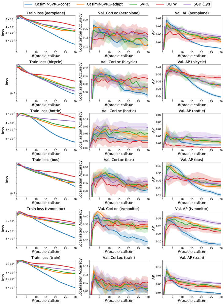
Figure 8: Comparison of convex optimization algorithms for the task of visual object localization on PASCAL VOC 2007 for $\lambda=10/n$ for all other classes (1/3).

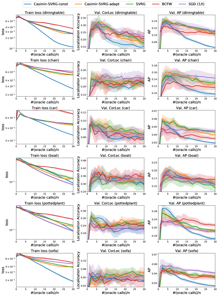
Figure 9: Comparison of convex optimization algorithms for the task of visual object localization on PASCAL VOC 2007 for $\lambda=10/n$ for all other classes (2/3).

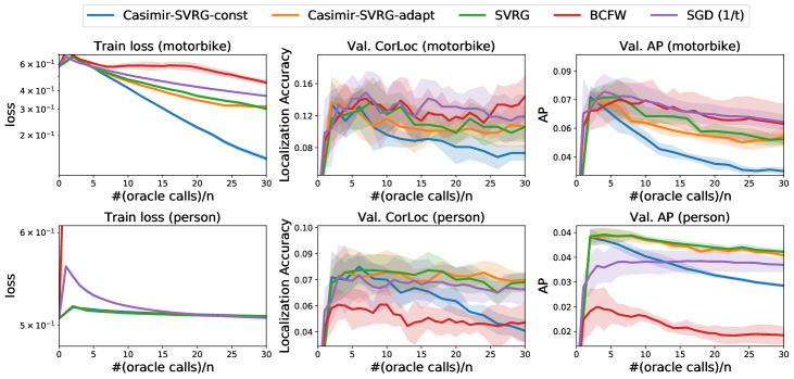
Figure 10: Comparison of convex optimization algorithms for the task of visual object localization on PASCAL VOC 2007 for $\lambda=10/n$ for all other classes (3/3).

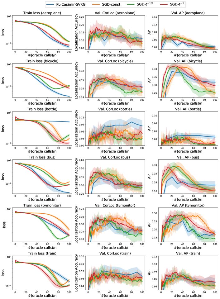
Figure 11: Comparison of non-convex optimization algorithms for the task of visual object localization on PASCAL VOC 2007 for $\lambda=1/n$ for all other classes (1/3).

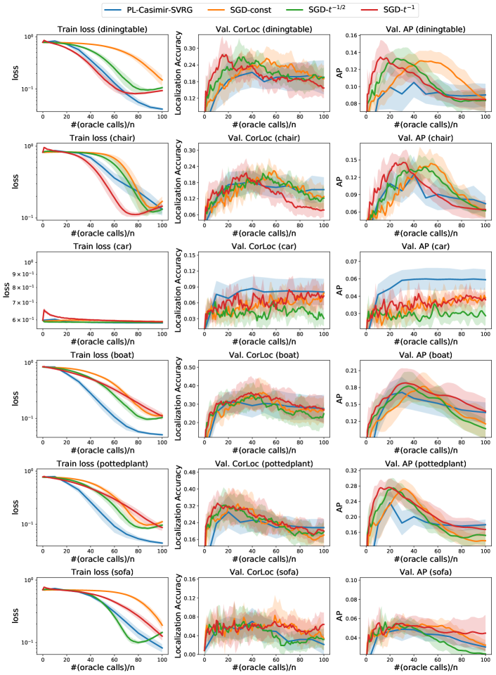
Figure 12: Comparison of non-convex optimization algorithms for the task of visual object localization on PASCAL VOC 2007 for $\lambda=1/n$ for all other classes (2/3).

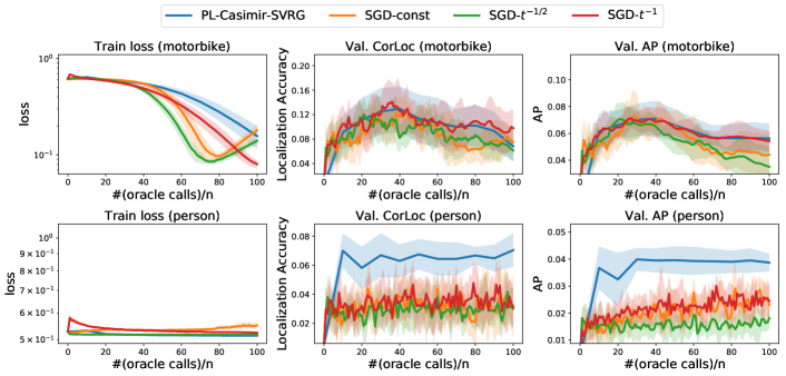
Figure 13: Comparison of non-convex optimization algorithms for the task of visual object localization on PASCAL VOC 2007 for $\lambda=1/n$ for all other classes (3/3).

References

- Allen-Zhu (2017) Z. Allen-Zhu. Katyusha: The First Direct Acceleration of Stochastic Gradient Methods. Journal of Machine Learning Research, 18:221:1–221:51, 2017.
- Altun et al. (2003) Y. Altun, I. Tsochantaridis, and T. Hofmann. Hidden Markov Support Vector Machines. In International Conference on Machine Learning, pages 3–10, 2003.
- Batra (2012) D. Batra. An efficient message-passing algorithm for the -best MAP problem. In Conference on Uncertainty in Artificial Intelligence, pages 121–130, 2012.
- Batra et al. (2012) D. Batra, P. Yadollahpour, A. Guzmán-Rivera, and G. Shakhnarovich. Diverse -best Solutions in Markov Random Fields. In European Conference on Computer Vision, pages 1–16, 2012.
- Beck and Teboulle (2012) A. Beck and M. Teboulle. Smoothing and first order methods: A unified framework. SIAM Journal on Optimization, 22(2):557–580, 2012.
- Belanger and McCallum (2016) D. Belanger and A. McCallum. Structured prediction energy networks. In International Conference on Machine Learning, pages 983–992, 2016.
- Bellman (1957) R. Bellman. Dynamic Programming. Courier Dover Publications, 1957.
- Bengio et al. (1995) Y. Bengio, Y. LeCun, C. Nohl, and C. Burges. LeRec: A NN/HMM Hybrid for On-Line Handwriting Recognition. Neural Computation, 7(6):1289–1303, 1995.
- Bertsekas (1995) D. P. Bertsekas. Dynamic programming and optimal control, volume 1. Athena scientific Belmont, MA, 1995.
- Bertsekas (1999) D. P. Bertsekas. Nonlinear programming. Athena Scientific Belmont, 1999.
- Bottou and Gallinari (1990) L. Bottou and P. Gallinari. A Framework for the Cooperation of Learning Algorithms. In Advances in Neural Information Processing Systems, pages 781–788, 1990.
- Bottou et al. (1997) L. Bottou, Y. Bengio, and Y. LeCun. Global Training of Document Processing Systems Using Graph Transformer Networks. In Conference on Computer Vision and Pattern Recognition, pages 489–494, 1997.
- Bradski (2000) G. Bradski. The OpenCV Library. Dr. Dobb’s Journal of Software Tools, 2000.
- Burke (1985) J. V. Burke. Descent methods for composite nondifferentiable optimization problems. Mathematical Programming, 33(3):260–279, 1985.
- Chen et al. (2013) C. Chen, V. Kolmogorov, Y. Zhu, D. N. Metaxas, and C. H. Lampert. Computing the Most Probable Modes of a Graphical Model. In International Conference on Artificial Intelligence and Statistics, pages 161–169, 2013.
- Cheng et al. (1996) Y.-Q. Cheng, V. Wu, R. Collins, A. R. Hanson, and E. M. Riseman. Maximum-weight bipartite matching technique and its application in image feature matching. In Visual Communications and Image Processing, volume 2727, pages 453–463, 1996.
- Collins et al. (2008) M. Collins, A. Globerson, T. Koo, X. Carreras, and P. L. Bartlett. Exponentiated gradient algorithms for conditional random fields and max-margin markov networks. Journal of Machine Learning Research, 9(Aug):1775–1822, 2008.
- Collobert et al. (2011) R. Collobert, J. Weston, L. Bottou, M. Karlen, K. Kavukcuoglu, and P. P. Kuksa. Natural language processing (almost) from scratch. Journal of Machine Learning Research, 12:2493–2537, 2011.
- Cooper (1990) G. F. Cooper. The computational complexity of probabilistic inference using bayesian belief networks. Artificial Intelligence, 42(2-3):393–405, 1990.
- Cox et al. (2014) B. Cox, A. Juditsky, and A. Nemirovski. Dual subgradient algorithms for large-scale nonsmooth learning problems. Mathematical Programming, 148(1-2):143–180, 2014.
- Crammer and Singer (2001) K. Crammer and Y. Singer. On the algorithmic implementation of multiclass kernel-based vector machines. Journal of Machine Learning Research, 2(Dec):265–292, 2001.
- Daumé III and Marcu (2005) H. Daumé III and D. Marcu. Learning as search optimization: approximate large margin methods for structured prediction. In International Conference on Machine Learning, pages 169–176, 2005.
- Davis and Drusvyatskiy (2018) D. Davis and D. Drusvyatskiy. Stochastic model-based minimization of weakly convex functions. arXiv preprint arXiv:1803.06523, 2018.
- Dawid (1992) A. P. Dawid. Applications of a general propagation algorithm for probabilistic expert systems. Statistics and Computing, 2(1):25–36, 1992.
- Defazio (2016) A. Defazio. A simple practical accelerated method for finite sums. In Advances in Neural Information Processing Systems, pages 676–684, 2016.
- Defazio et al. (2014) A. Defazio, F. Bach, and S. Lacoste-Julien. SAGA: A fast incremental gradient method with support for non-strongly convex composite objectives. In Advances in Neural Information Processing Systems, pages 1646–1654, 2014.
- Deselaers et al. (2010) T. Deselaers, B. Alexe, and V. Ferrari. Localizing objects while learning their appearance. In European Conference on Computer Vision, pages 452–466, 2010.
- Drusvyatskiy and Paquette (2018) D. Drusvyatskiy and C. Paquette. Efficiency of minimizing compositions of convex functions and smooth maps. Mathematical Programming, Jul 2018.
- Duchi et al. (2006) J. C. Duchi, D. Tarlow, G. Elidan, and D. Koller. Using Combinatorial Optimization within Max-Product Belief Propagation. In Advances in Neural Information Processing Systems, pages 369–376, 2006.
- Everingham et al. (2010) M. Everingham, L. Van Gool, C. K. Williams, J. Winn, and A. Zisserman. The Pascal Visual Object Classes (VOC) challenge. International Journal of Computer Vision, 88(2):303–338, 2010.
- Flerova et al. (2016) N. Flerova, R. Marinescu, and R. Dechter. Searching for the Best Solutions in Graphical Models. Journal of Artificial Intelligence Research, 55:889–952, 2016.
- Fromer and Globerson (2009) M. Fromer and A. Globerson. An LP view of the -best MAP problem. In Advances in Neural Information Processing Systems, pages 567–575, 2009.
- Frostig et al. (2015) R. Frostig, R. Ge, S. Kakade, and A. Sidford. Un-regularizing: approximate proximal point and faster stochastic algorithms for empirical risk minimization. In International Conference on Machine Learning, pages 2540–2548, 2015.
- Girshick et al. (2014) R. Girshick, J. Donahue, T. Darrell, and J. Malik. Rich feature hierarchies for accurate object detection and semantic segmentation. In Conference on Computer Vision and Pattern Recognition, pages 580–587, 2014.
- Greig et al. (1989) D. M. Greig, B. T. Porteous, and A. H. Seheult. Exact maximum a posteriori estimation for binary images. Journal of the Royal Statistical Society. Series B (Methodological), pages 271–279, 1989.
- Hazan and Urtasun (2010) T. Hazan and R. Urtasun. A Primal-Dual Message-Passing Algorithm for Approximated Large Scale Structured Prediction. In Advances in Neural Information Processing Systems, pages 838–846, 2010.
- Hazan et al. (2016) T. Hazan, A. G. Schwing, and R. Urtasun. Blending Learning and Inference in Conditional Random Fields. Journal of Machine Learning Research, 17:237:1–237:25, 2016.
- He et al. (2017) L. He, K. Lee, M. Lewis, and L. Zettlemoyer. Deep Semantic Role Labeling: What Works and What’s Next. In Annual Meeting of the Association for Computational Linguistics, pages 473–483, 2017.
- He and Harchaoui (2015) N. He and Z. Harchaoui. Semi-Proximal Mirror-Prox for Nonsmooth Composite Minimization. In Advances in Neural Information Processing Systems, pages 3411–3419, 2015.
- Held et al. (1974) M. Held, P. Wolfe, and H. P. Crowder. Validation of subgradient optimization. Mathematical Programming, 6(1):62–88, Dec 1974.
- Hofmann et al. (2015) T. Hofmann, A. Lucchi, S. Lacoste-Julien, and B. McWilliams. Variance reduced stochastic gradient descent with neighbors. In Advances in Neural Information Processing Systems, pages 2305–2313, 2015.
- Ishikawa and Geiger (1998) H. Ishikawa and D. Geiger. Segmentation by grouping junctions. In Conference on Computer Vision and Pattern Recognition, pages 125–131, 1998.
- Jerrum and Sinclair (1993) M. Jerrum and A. Sinclair. Polynomial-time approximation algorithms for the Ising model. SIAM Journal on computing, 22(5):1087–1116, 1993.
- Joachims et al. (2009) T. Joachims, T. Finley, and C.-N. J. Yu. Cutting-plane training of structural SVMs. Machine Learning, 77(1):27–59, 2009.
- Johnson (2008) J. K. Johnson. Convex relaxation methods for graphical models: Lagrangian and maximum entropy approaches. PhD thesis, Massachusetts Institute of Technology, Cambridge, MA, USA, 2008.
- Johnson and Zhang (2013) R. Johnson and T. Zhang. Accelerating stochastic gradient descent using predictive variance reduction. In Advances in Neural Information Processing Systems, pages 315–323, 2013.
- Jojic et al. (2010) V. Jojic, S. Gould, and D. Koller. Accelerated dual decomposition for MAP inference. In International Conference on Machine Learning, pages 503–510, 2010.
- Jurafsky et al. (2014) D. Jurafsky, J. H. Martin, P. Norvig, and S. Russell. Speech and Language Processing. Pearson Education, 2014. ISBN 9780133252934.
- Koller and Friedman (2009) D. Koller and N. Friedman. Probabilistic Graphical Models - Principles and Techniques. MIT Press, 2009. ISBN 978-0-262-01319-2.