Symmetries of spatial meson correlators in high temperature QCD

Abstract

Based on a complete set of $J=0$ and $J=1$ spatial isovector correlation functions calculated with $N_{F}=2$ domain wall fermions we identify an intermediate temperature regime of $T\sim 220-500$ MeV ($1.2T_{c}$–$2.8T_{c}$), where chiral symmetry is restored but the correlators are not yet compatible with a simple free quark behavior. More specifically, in the temperature range $T\sim 220-500$ MeV we identify a multiplet structure of spatial correlators that suggests emergent $SU(2)_{CS}$ and $SU(4)$ symmetries, which are not symmetries of the free Dirac action. The symmetry breaking effects in this temperature range are less than 5%. Our results indicate that at these temperatures the chromo-magnetic interaction is suppressed and the elementary degrees of freedom are chirally symmetric quarks bound into color-singlet objects by the chromo-electric component of the gluon field. At temperatures between 500 and 660 MeV the emergent $SU(2)_{CS}$ and $SU(4)$ symmetries disappear and one observes a smooth transition to the regime above $T\sim 1$ GeV where only chiral symmetries survive, which are finally compatible with quasi-free quarks.

I Introduction

Understanding the physics of strongly coupled matter at high temperature is one of the great open challenges in high energy physics. Addressing this question is the subject of large-scale experimental and theoretical efforts. Initially it was assumed that above some pseudo-critical temperature $T_{c}$ quarks deconfine and chiral symmetry is restored such that above $T_{c}$ the degrees of freedom are liberated quarks and gluons Sh .

A flavor non-singlet chiral restoration was indeed confirmed on the lattice, which is signalled by the vanishing quark condensate above the cross-over region around $T_{c}$ and by degeneracy of correlators that are connected by chiral transformations.

The expected confinement-deconfinement transition turned out to be more intricate to define. Such a transition was historically assumed to be associated with a different expectation value of the Polyakov loop P ; L below and above the critical temperature $T_{c}$. In pure $SU(3)$ gauge theory the Polyakov loop is connected with the $Z_{3}$ center symmetry and indeed a sharp first-order phase transition is observed Kaczmarek:2002mc , which indicates that the relevant degrees of freedom below and above $T_{c}$ are different. Still, one may ask whether this $Z_{3}$ transition is really connected with deconfinement in a pure glue theory. Traditionally the answer was affirmative, because the expectation value of the Polyakov loop can be related to the free energy of a static quark source. If this energy is infinite, which corresponds to a vanishing Polyakov loop, then we are in a confining mode, while deconfinement should be associated with a finite free energy, i.e., a non-zero Polyakov loop. However, this argumentation is self-contradictory because a criterion for deconfinement in pure gauge theory, i.e., deconfinement of gluons, is reduced to deconfinement of a static charge (heavy quark), that is not part of the pure glue theory. The Polyakov loop is a valid order parameter but strictly speaking its relation to confinement is an assumption. And indeed, just above the first-order $Z_{3}$ phase transition the energy and pressure are quite different from the Stefan-Boltzmann limit which is associated with free deconfined gluons b .

In a theory with dynamical quarks the first-order phase transition is washed out and on the lattice one observes a very smooth increase of the Polyakov loop Petreczky:2015yta . The reason for that behavior is rather clear: in a theory with dynamical quarks there is no $Z_{3}$ symmetry and the Polyakov loop ceases to be an order parameter. Considering the finite energy of a pair of static quark sources (Polyakov loop correlator) the resulting string breaking potential is due to vacuum loops of light quarks that combine with the static sources to a pair of heavy-light mesons. Lattice measurements of the energy density and pressure with dynamical quarks indicate a smooth transition, and at $T\sim 1$ GeV the system is still quite far from the Stefan-Boltzmann limit Karsch:2000ps ; Bazavov:2017dsy .

In view of the absence of a reliable, generally accepted definition and order parameter for deconfinement – except for the most straightforward statement that confinement is the absence of colored states in the spectrum – a key to understanding the nature of hot QCD matter is information about the relevant effective degrees of freedom in high temperature QCD. Several model and lattice studies suggest the possible existence of inter-quark correlations or bound states above $T_{c}$, see, e.g., Refs. Shuryak:2003ty ; Ratti:2011au ; Mukherjee:2015mxc . While models may provide helpful intuitive understanding, it is important to attempt finding model independent ways to identify the degrees of freedom in high T QCD.

Among other observables, relevant information is encoded in Euclidean correlation functions. At zero temperature hadron masses can be extracted from the exponential slope of correlators in the Euclidean time direction $t$. At non-zero temperature the temporal extent is finite by definition (it vanishes at $T\rightarrow\infty$) such that there is no strict notion of an asymptotic behavior for $t$-correlators. Spatial correlators on the other hand are well-defined and do provide detailed information about the QCD dynamics DeTar:1987xb ; Born:1991zz ; Fl ; Kogut:1998rh ; Pushkina:2004wa ; Wi ; Gavai:2006fs ; Cheng:2010fe ; Banerjee:2011yd . These spatial correlators can be analyzed with respect to the symmetries they exhibit, which in turn allows one to extract information about the relevant effective degrees of freedom.

In previous work Rohrhofer:2017grg we have studied a complete set of $J=0$ and $J=1$ isovector correlation functions in $z$-direction for a system with $N_{F}=2$ dynamical quarks in simulations with the chirally symmetric domain wall Dirac operator at temperatures up to $T\sim 380$ MeV. Similar ensembles have been used previously for the study of the $U(1)_{A}$ restoration in $t$-correlators and via the Dirac eigenvalue decomposition of correlators Cossu:2015kfa ; Tomiya:2016jwr . We have observed the restoration of both $SU(2)_{L}\times SU(2)_{R}$ and $U(1)_{A}$ chiral symmetries at $T_{c}$ on a finite lattice of a given size.

However, by analyzing the formation of multiplets for the spatial correlators even larger symmetries, referred to as $SU(2)_{CS}$ chiral spin and $SU(4)$ symmetries G1 ; GP , have been identified in the $J=1$ correlators in the region $T\sim 2\,T_{c}$. These symmetries, while not symmetries of the Dirac Lagrangian, are symmetries of the Lorentz-invariant fermion charge. In the given reference frame they are symmetries of the interaction between the chromo-electric field with the quarks while the interaction of quarks with the chromo-magnetic field breaks them. These symmetries include as subgroups the chiral symmetries as well as rotations between the right- and left-handed components of quarks. Such symmetries have been found already earlier in the hadron spectrum at zero temperature D1 ; D2 ; D3 ; D4 upon artificial truncation of the near-zero modes of the Dirac operator LS . While the $SU(2)_{L}\times SU(2)_{R}$ and $U(1)_{A}$ chiral symmetries are almost exact above $T_{c}$, the $SU(2)_{CS}$ and $SU(4)$ symmetries are approximate. In this paper we improve the analysis and extend the temperature range up to $T\sim 1$ GeV, in order to further study the temperature evolution of the symmetries of correlators and thus the temperature evolution of the emergent effective degrees of freedom.

We stress that the $SU(2)_{CS}$ and $SU(4)$ symmetries are not symmetries of the free Dirac action and therefore their emergence is incompatible with the notion of quasi-free, deconfined quarks. The emergence of these symmetries in a range from $T\sim 220$ – $500$ MeV ($1.2T_{c}$ – $2.8T_{c}$), as reported in this article, suggests that the effective degrees of freedom of QCD at these temperatures are quarks with definite chirality bound by the chromo-electric component of the gluon field into color-singlet objects, “string-like” compounds.

While the lattice study is possible only at zero chemical potential, the observed approximate symmetries should persist also at finite chemical potential, due to the quark chemical potential term in the QCD action being manifestly $SU(2)_{CS}$ and $SU(4)$ symmetric G2 .

When increasing the temperature to $T\sim 1$ GeV we observe that at very high temperature the $SU(2)_{CS}$ and $SU(4)$ multiplet structure is washed out and the full QCD meson correlators approach the corresponding correlators constructed with free, non-interacting quarks. This indicates that at very high temperature the coupling constant is sufficiently small to describe dynamics of weakly interacting quarks and gluons. Preliminary results of this work were presented at the Lattice 2018 conference Rohrhofer:2018pey .

II Spatial finite temperature meson correlators for non-interacting quarks in the continuum

We begin our presentation with a summary of the calculation of the spatial correlators for free massless quarks in the continuum. This situation is the limiting case that should represent QCD at very high temperatures where, due to asymptotic freedom, the interaction via gluons can be neglected. We discuss the multiplet structure for this reference case which we will later use to compare to our lattice calculation at high, but not asymptotically high temperature. In particular we will find that at moderately high temperatures above $T_{c}$ the spatial correlators of full QCD display a multiplet structure different from the limiting case of free quarks discussed in this section. We remark that some of the free spatial continuum correlators computed here were already presented in Fl ; Wi , but for a systematical and complete discussion we need the full set of all spatial meson correlators and thus briefly summarize their derivation in this section and the appendix.

In the continuum the free spatial meson correlators in infinite spatial volume are given by

$$C_{\Gamma}(z)\;=\;\int_{-\infty}^{\infty}\!\!dx\int_{-\infty}^{\infty}\!\!dy\int_{0}^{\beta}\!\!dt\;\left\langle{\cal O}_{\Gamma}(x,y,z,t)\;{\cal O}_{\Gamma}(0,0,0,0)^{\dagger}\right\rangle\;.$$ (1)

We consider Euclidean space at finite temperature, i.e., $x,y,z\in\mathds{R}$, and $t\in[0,\beta)$, where $\beta$ is the inverse temperature. In the correlators (1) we look at correlation in one of the spatial directions, here chosen as $z$, while the other two, $x$ and $y$, as well as the Euclidean time $t$ are integrated over. The latter integration over all coordinates that are perpendicular to the direction of propagation, i.e., the $z$-direction, fixes a “Euclidean rest frame” for our correlators.

The meson interpolators are given by

$${\cal O}_{\Gamma}({\bf x})\;\equiv\;\overline{u}({\bf x})\Gamma d({\bf x})\;,\quad{\cal O}_{\Gamma}({\bf 0})^{\dagger}\;\equiv\;-\;\overline{d}({\bf 0})\Gamma^{\dagger}u({\bf 0})\;,$$ (2)

where we use the abbreviations ${\bf x}=(x,y,z,t)$ and ${\bf 0}=(0,0,0,0)$, and $\Gamma$ is an element of the Clifford algebra, i.e., a product of $\gamma$ matrices (see below). Note that choosing the negative sign for ${\cal O}_{\Gamma}^{\dagger}$ is a definition, since in general the sign obtained from conjugation will depend on $\Gamma$. Throughout the whole paper we use the set $\gamma_{\mu},\mu=1,2,3,4$ of Euclidean $\gamma$-matrices that satisfy the anti-commutation relations

$$\gamma_{\mu}\gamma_{\nu}+\gamma_{\nu}\gamma_{\mu}\;=\;2\delta_{\mu\nu}\;,\;\qquad\gamma_{5}\;\equiv\;\gamma_{1}\gamma_{2}\gamma_{3}\gamma_{4}\;.$$ (3)

$\overline{u}({\bf x})$, $u({\bf x})$, $\overline{d}({\bf x})$, $d({\bf x})$ are free massless Dirac spinors which obey anti-periodic boundary conditions in Euclidean time. We remark that for simplicity we here have already expressed the non-singlet correlators in terms of the flavor spinors $u$ and $d$, while in the next section we write them in terms of isospin doublets $q({\bf x})\equiv(u({\bf x}),d({\bf x}))$. After contracting the fermions, the two forms for writing the non-singlet bilinears of course give the same expressions.

Performing these contractions we obtain

$$\left\langle{\cal O}_{\Gamma}({\bf x})\;{\cal O}_{\Gamma}({\bf 0})^{\dagger}\right\rangle\;=\;\mbox{Tr}\,\big{[}S({\bf x},{\bf 0})\,\Gamma^{\dagger}S({\bf 0},{\bf x})\,\Gamma\big{]}\;,$$ (4)

where the trace is over Dirac indices and $S$ denotes the free continuum Dirac propagator. We are interested in the physics near the chiral limit, and therefore we consider massless quarks in this section. In terms of Fourier integrals $S$ is given by

$$S({\bf x},{\bf x}^{\prime})\;=\;\frac{1}{(2\pi)^{3}\beta}\int_{-\infty}^{\infty}\!\!\!\!dp_{x}\int_{-\infty}^{\infty}\!\!\!\!dp_{y}\int_{-\infty}^{\infty}\!\!\!\!dp_{z}\sum_{n\in\mathds{Z}}\,i\,\frac{\cancel{\bf p}}{{\bf p}^{2}}\,e^{\,i\,{\bf p}\,({\bf x}-{\bf x}^{\prime})}\;,$$ (5)

where ${\bf p}=(p_{x},p_{y},p_{z},\omega_{n})$, with the Matsubara frequencies $\omega_{n}=\pi(2n+1)/\beta$. Inserting (5) into (4) and this into (1) we find

$$C_{\Gamma}(z)\;=\;-\frac{1}{(2\pi)^{4}\beta}\int_{-\infty}^{\infty}\!\!\!\!dp_{x}\int_{-\infty}^{\infty}\!\!\!\!dp_{y}\sum_{n\in\mathds{Z}}\int_{-\infty}^{\infty}\!\!\!\!dp_{z}\,\frac{e^{izp_{z}}}{{\bf p}^{2}}\int_{-\infty}^{\infty}\!\!\!\!dp_{z}^{\prime}\,\frac{e^{-izp_{z}^{\prime}}}{\widetilde{\bf p}^{\,2}}\;\mbox{Tr}\big{[}\,\cancel{\bf p}\,\Gamma^{\dagger}\,\widetilde{\cancel{\bf p}}\,\Gamma\,\big{]},$$ (6)

where $\widetilde{\bf p}\equiv(p_{x},p_{y},p_{z}^{\prime},\omega_{n})$ and we have already integrated over $x$, $y$ and $t$ in (1) which generated two Dirac deltas and a Kronecker delta that were used to get rid of two of the momentum integrals and one of the Matsubara sums.

As we will see below, the trace in the integrand has the general form

$$\mbox{Tr}\big{[}\,\cancel{\bf p}\,\Gamma^{\dagger}\,\widetilde{\cancel{\bf p}}\,\Gamma\,\big{]}\;=\;4\big{[}\,s_{x}\,p_{x}^{2}\,+\,s_{y}\,p_{y}^{2}\,+\,s_{z}\,p_{z}\,p_{z}^{\prime}\,+\,s_{\tau}\,\omega_{n}^{2}\,\big{]}\;,$$ (7)

where $s_{x},s_{y},s_{z}$ and $s_{\tau}$ are signs that depend on the choice of $\Gamma$. Thus for the pair of integrals over the $z$ components we can distinguish two cases, depending on whether the factor $p_{z}\,p_{z}^{\prime}$ appears in the integrand or not,

$$\int_{-\infty}^{\infty}\!\!\!\!dp_{z}\,\frac{e^{izp_{z}}}{p_{z}^{2}+\Omega^{2}}\int_{-\infty}^{\infty}\!\!\!\!dp_{z}^{\prime}\,\frac{e^{-izp_{z}^{\prime}}}{{p_{z}^{\prime}}^{2}+\Omega^{2}}\;=\;\left[\int_{-\infty}^{\infty}\!\!\!\!dp_{z}\,\frac{e^{izp_{z}}}{p_{z}^{2}+\Omega^{2}}\right]^{2}\;\equiv\;I_{0}^{\,2}\;,$$ (8)

$$\int_{-\infty}^{\infty}\!\!\!\!dp_{z}\,\frac{e^{izp_{z}}\,p_{z}}{p_{z}^{2}+\Omega^{2}}\int_{-\infty}^{\infty}\!\!\!\!dp_{z}^{\prime}\,\frac{e^{-izp_{z}^{\prime}}\,p_{z}^{\prime}}{{p_{z}^{\prime}}^{2}+\Omega^{2}}\;=\;-\left[\int_{-\infty}^{\infty}\!\!\!\!dp_{z}\,\frac{e^{izp_{z}}\,p_{z}}{p_{z}^{2}+\Omega^{2}}\right]^{2}\;\equiv\;-I_{1}^{\,2}\;,$$ (9)

where we have defined $\Omega=\sqrt{p_{x}^{2}+p_{y}^{2}+\omega_{n}^{2}}$. The integrals $I_{0}$ and $I_{1}$ are straightforward to solve with the residue theorem,

$$I_{0}^{\,2}\;=\;\frac{\pi^{2}}{\Omega^{2}}\,e^{\,-z\,2\Omega}\;,\quad-I_{1}^{\,2}\;=\;\pi^{2}\,e^{\,-z\,2\Omega}\;.$$ (10)

We find for the correlator $C_{\Gamma}(z)$,

$$C_{\Gamma}(z)\;=\;-\big{[}\,s_{x}\,C_{s}(z)\,+\,s_{y}\,C_{s}(z)\,+\,s_{z}\,C_{z}(z)\,+\,s_{\tau}\,C_{\tau}(z)\,\big{]}\;,$$ (11)

with the individual correlators given by

$$C_{s}(z) = \frac{1}{(2\pi)^{2}\beta}\sum_{n\in\mathds{Z}}\int_{-\infty}^{\infty}\!\!\!\!dp_{x}\int_{-\infty}^{\infty}\!\!\!\!dp_{y}\;\frac{e^{\,-2\,z\sqrt{p_{x}^{2}+p_{y}^{2}+\omega_{n}^{2}}}}{p_{x}^{2}+p_{y}^{2}+\omega_{n}^{2}}\,p_{x}^{2}\;,$$ (12)

$$C_{z}(z) = \frac{1}{(2\pi)^{2}\beta}\sum_{n\in\mathds{Z}}\int_{-\infty}^{\infty}\!\!\!\!dp_{x}\int_{-\infty}^{\infty}\!\!\!\!dp_{y}\;e^{\,-2\,z\sqrt{p_{x}^{2}+p_{y}^{2}+\omega_{n}^{2}}}\;,$$

$$C_{\tau}(z) = \frac{1}{(2\pi)^{2}\beta}\sum_{n\in\mathds{Z}}\int_{-\infty}^{\infty}\!\!\!\!dp_{x}\int_{-\infty}^{\infty}\!\!\!\!dp_{y}\;\frac{e^{\,-2\,z\sqrt{p_{x}^{2}+p_{y}^{2}+\omega_{n}^{2}}}}{p_{x}^{2}+p_{y}^{2}+\omega_{n}^{2}}\,\omega_{n}^{\,2}\;.$$

The correlators $C_{s}(z),C_{z}(z)$ and $C_{\tau}(z)$ obey the obvious sum rule

$$2\,C_{s}(z)\;+\;C_{\tau}(z)\;=\;C_{z}(z)\;,$$ (13)

i.e., only two of them are independent. We choose $C_{z}(z)$ and $C_{\tau}(z)$ to express all other correlators. The treatment of the Matsubara sums and the necessary integrals for evaluating $C_{z}(z)$ and $C_{\tau}(z)$ are discussed in Appendix A, where we also discuss the asymptotic behavior of the correlators.

We now come to the identification of multiplets, i.e., we identify the sets of Clifford algebra elements $\Gamma$ that share the same decay properties for their corresponding correlators $C_{\Gamma}(z)$. For this we need to determine the signs $s_{x},s_{y},s_{z}$ and $s_{\tau}$ in the traces (7) for the different choices of $\Gamma$, which in turn determine how the respective correlator $C_{\Gamma}(z)$ is composed from the contributions $C_{s}(z)$, $C_{z}(z)$ and $C_{\tau}(z)$ according to (11).

We first note that for chiral partners, i.e., correlators where $\Gamma$ is replaced by $\Gamma\gamma_{5}$, the corresponding correlators $C_{\Gamma}(z)$ and $C_{\Gamma\gamma_{5}}(z)$ have opposite overall signs, and thus also opposite individual signs $s_{x},s_{y},s_{z}$ and $s_{\tau}$. This follows from the trivial relation

$$\mbox{Tr}\big{[}\,\cancel{\bf p}\,(\Gamma\gamma_{5})^{\dagger}\,\widetilde{\cancel{\bf p}}\,\Gamma\gamma_{5}\,\big{]}\;=\;-\;\mbox{Tr}\big{[}\,\cancel{\bf p}\,\Gamma^{\dagger}\,\widetilde{\cancel{\bf p}}\,\Gamma\,\big{]}\;.$$ (14)

This implies that we need to determine the signs $s_{x},s_{y},s_{z}$ and $s_{\tau}$ in the traces (7) only for 8 out of the 16 Clifford algebra generators $\Gamma$. Our results for the signs $s_{x},s_{y},s_{z}$ and $s_{\tau}$ that determine the decomposition of $\mbox{Tr}\big{[}\,\cancel{\bf p}\,\Gamma^{\dagger}\,\widetilde{\cancel{\bf p}}\,\Gamma\,\big{]}$ according to (7) are listed in Table 1.

$\;\,\Gamma$	$\!\!\!s_{x}$	$\!\!\!s_{y}$	$\!\!\!s_{z}$	$\!\!\!s_{\tau}$	name	chiral partner
$\mathds{1}$	$+$	$+$	$+$	$+$	$S$	$PS$
$\!\gamma_{1}$	$+$	$-$	$-$	$-$	$V_{x}$	$A_{x}$
$\gamma_{2}$	$-$	$+$	$-$	$-$	$V_{y}$	$A_{y}$
$\gamma_{4}$	$-$	$-$	$-$	$+$	$V_{t}$	$A_{t}$
$\!\gamma_{1}\gamma_{3}$	$-$	$+$	$-$	$+$	$T_{x}$	$X_{x}$
$\gamma_{2}\gamma_{3}$	$+$	$-$	$-$	$+$	$T_{y}$	$X_{y}$
$\gamma_{4}\gamma_{3}$	$+$	$+$	$-$	$-$	$T_{t}$	$X_{t}$
$\gamma_{3}$	$-$	$-$	$+$	$-$

Table 1: The signs $s_{x}$, $s_{y}$ $s_{z}$ and $s_{\tau}$ that determine the trace $\mbox{Tr}\big{[}\,\cancel{\bf p}\,\Gamma^{\dagger}\,\widetilde{\cancel{\bf p}}\,\Gamma\,\big{]}$ for different choices of $\Gamma$ according to (7). For chiral partners, i.e., when $\Gamma$ is replaced by $\Gamma\gamma_{5}$, all signs are reversed (compare (14)). To simplify the notation we chose the (irrelevant) overall signs equal for both chiral partners such that the relative signs $s_{x}$, $s_{y}$ $s_{z}$ and $s_{\tau}$ as listed in the table are used for both chiral partners. In the two columns on the right we give the names of the bilinears and their chiral partners which we will discuss in detail in the next section. Since the interpolators with $\gamma_{3}$ and $\gamma_{3}\gamma_{5}$ vanish identically no name is assigned.

Having determined the signs $s_{x},s_{y},s_{z},s_{\tau}$ we use them in (11) to work out the composition of $C_{\Gamma}(z)$ from the building blocks $C_{s}(z)$, $C_{z}(z)$ and $C_{\tau}(z)$, and after eliminating $C_{s}(z)$ we obtain the representation for the $C_{\Gamma}(z)$ in terms of $C_{z}(z)$ and $C_{\tau}(z)$ evaluated in Appendix A. We find (overall signs were chosen such that chiral partners have the same overall sign),

$$\;\;C_{\mathds{1}}(z)=C_{\gamma_{5}}(z)\;=\;2C_{s}(z)\,+\,C_{z}(z)\,+\,C_{\tau}(z)\;=\;2\,C_{z}(z)\;,$$ (15)

$$\;\;C_{\gamma_{1}}(z)=C_{\gamma_{1}\gamma_{5}}(z)=C_{\gamma_{2}}(z)=C_{\gamma_{2}\gamma_{5}}(z)\;=\;C_{z}(z)+C_{\tau}(z)\;,$$

$$\;\;C_{\gamma_{4}}(z)=C_{\gamma_{4}\gamma_{5}}(z)=\;2C_{s}(z)+C_{z}(z)-C_{\tau}(z)\;=\;2(C_{z}(z)-C_{\tau}(z))\;,$$

$$\;\;C_{\gamma_{1}\gamma_{3}}(z)=C_{\gamma_{1}\gamma_{3}\gamma_{5}}(z)=C_{\gamma_{2}\gamma_{3}}(z)=C_{\gamma_{2}\gamma_{3}\gamma_{5}}(z)\;=\;C_{z}(z)-C_{\tau}(z)\;,$$

$$\;\;C_{\gamma_{4}\gamma_{3}}(z)=C_{\gamma_{4}\gamma_{3}\gamma_{5}}(z)=\;-2C_{s}(z)+C_{z}(z)+C_{\tau}(z)\;=\;2\,C_{\tau}(z)\;,$$

$$\;\;C_{\gamma_{3}}(z)=C_{\gamma_{3}\gamma_{5}}(z)\;=\;2C_{s}(z)\,-\,C_{z}(z)\,+\,C_{\tau}(z)\;=\;0\;.$$

The vanishing of the correlators $C_{\gamma_{3}}(z)$ and $C_{\gamma_{3}\gamma_{5}}(z)$ is a direct consequence of the sum rule (13). From a more physical point of view this vanishing is a consequence of current conservation. Indeed $C_{\gamma_{3}}(z)$ is the correlator for the 3-component of the conserved vector current $J_{\mu}({\bf x})=\overline{u}({\bf x})\,\gamma_{\mu}d({\bf x})$ and concerning the propagation in $z$-direction the integral $\int\!\!dxdydt\,J_{3}(x,y,z,t)$ is a conserved charge. Thus the corresponding spatial correlator and its chiral partner vanish, which also implies that the sum rule (13) is directly linked to current conservation. Furthermore the sum rule (current conservation) means that the correlators $C_{\gamma_{4}}(z)=C_{\gamma_{4}\gamma_{5}}(z)$ are not independent from the correlators $C_{\gamma_{1}\gamma_{3}}(z)=C_{\gamma_{1}\gamma_{3}\gamma_{5}}(z)=C_{\gamma_{2}\gamma_{3}}(z)=C_{\gamma_{2}\gamma_{3}\gamma_{5}}(z)$.

We conclude this section with quoting the asymptotic behavior of our correlators, which is obtained by using (65) from Appendix A in the expressions (15),

$$C_{\mathds{1}}(z)=\frac{2\pi}{\beta^{3}}\frac{e^{\,-\,2\,z\,\omega_{0}}}{2\,z\,\omega_{0}}\left[1+\frac{1}{2\,z\,\omega_{0}}\right]+O\!\left(\frac{e^{\,-\,4\,z\,\omega_{0}}}{z\omega_{0}}\right),$$

$$C_{\gamma_{1}}(z)=C_{\gamma_{2}}(z)=\frac{2\pi}{\beta^{3}}\frac{e^{\,-\,2\,z\,\omega_{0}}}{2\,z\,\omega_{0}}\left[1+\frac{1}{(2\,z\,\omega_{0})^{2}}+...\right]+O\!\left(\frac{e^{\,-\,4\,z\,\omega_{0}}}{z\omega_{0}}\right),$$

$$C_{\gamma_{4}}(z)=\frac{4\pi}{\beta^{3}}\frac{e^{\,-\,2\,z\,\omega_{0}}}{(2\,z\,\omega_{0})^{2}}\left[1-\frac{1}{2\,z\,\omega_{0}}+...\right]+O\!\left(\frac{e^{\,-\,4\,z\,\omega_{0}}}{z\omega_{0}}\right),$$

$$C_{\gamma_{1}\gamma_{3}}(z)=C_{\gamma_{2}\gamma_{3}}(z)=\frac{2\pi}{\beta^{3}}\frac{e^{\,-\,2\,z\,\omega_{0}}}{(2\,z\,\omega_{0})^{2}}\left[1-\frac{1}{2\,z\,\omega_{0}}+...\right]+O\!\left(\frac{e^{\,-\,4\,z\,\omega_{0}}}{z\omega_{0}}\right)\!,$$

$$C_{\gamma_{4}\gamma_{3}}(z)=\frac{2\pi}{\beta^{3}}\frac{e^{\,-\,2\,z\,\omega_{0}}}{2\,z\,\omega_{0}}\left[1-\frac{1}{2\,z\,\omega_{0}}+...\right]+O\!\left(\frac{e^{\,-\,6\,z\,\omega_{0}}}{z\omega_{0}}\right),$$

$$C_{\gamma_{3}}(z)=0\;.$$ (16)

Here we have only listed half of the correlators in each chiral multiplet without their chiral partners, which have identical correlators (up to an overall sign which we dropped). The fact that on the rhs. of (16) appears only the dimensionless combination $z\omega_{0}=\pi\,z/\beta=\pi\,zT$ reflects the absence of any physical scale in the conformal theory of massless non-interacting quarks.

III Fermionic bilinears and their symmetries

Having summarized the explicit form of the spatial correlators for the free case, let us now come to the general (full QCD) discussion of the mesonic bilinears and their symmetries. We are interested in the spatial correlators of the local isovector mesonic bilinears

$$\mathcal{O}_{\Gamma}(x)\;=\;\bar{q}(x)\,\Gamma\,\frac{\vec{\tau}}{2}\,q(x)\;,$$ (17)

which we now write using the isospin doublets $q(x)\equiv(u(x),d(x))$. The isovector structure of the bilinears is determined by the isospin Pauli matrices $\tau_{a}$. Again $\Gamma$ may be any element of the Clifford algebra and the choice of $\Gamma$ determines the symmetry properties of the respective bilinear.

Two $J=0$ bilinears can be defined by the following choices for $\Gamma$:

$$\Gamma=\left\{\begin{array}[]{cccl}\gamma_{5}&\quad\dots&PS&\quad(Pseudoscalar)\;,\\ \mathds{1}&\quad\dots&S&\quad(Scalar)\;.\end{array}\right.$$ (20)

These two bilinears can be transformed into each other by global ${U}(1)_{A}$ rotations

$$q(x)\rightarrow\exp\left(i\gamma_{5}\theta\right)q(x)\;.$$ (21)

For $J=1$ we consider bilinears with the following choices of $\Gamma$ that define the Vector bilinears $\mathbf{V}$:

$$\Gamma=\left\{\begin{array}[]{cccl}\gamma_{1}&\quad\dots&V_{x}\;,&\\ \gamma_{2}&\quad\dots&V_{y}\;,&\quad\textrm{({\it Vector})}\\ \gamma_{4}&\quad\dots&V_{t}\;.&\end{array}\right.$$ (25)

As we have already seen for the free case which we discussed in the previous section, due to current conservation the 3-component $\bar{q}(x)\gamma_{3}\frac{\vec{\tau}}{2}q(x)$ does not propagate in the $z$ direction such that we omit the choice $\Gamma=\gamma_{3}$.

The vector bilinears are related to their chiral partners through flavor non-singlet axial rotations

$$q(x)\rightarrow\exp\left(\frac{i}{2}\gamma_{5}\vec{\tau}\vec{\theta}\right)q(x)\;.$$ (26)

Their chiral partners, the Axial-vector bilinears $\mathbf{A}$ are defined as:

$$\Gamma=\left\{\begin{array}[]{cccl}\gamma_{1}\gamma_{5}&\quad\dots&A_{x}\;,&\\ \gamma_{2}\gamma_{5}&\quad\dots&A_{y}\;,&\quad\textrm{({\it Axial-vector})}\\ \gamma_{4}\gamma_{5}&\quad\dots&A_{t}\;.&\end{array}\right.$$ (30)

At zero (or sufficiently small) temperature the chiral partner of the non-propagating third vector current component, i.e., the bilinear with the gamma structure $\Gamma=\gamma_{3}\gamma_{5}$, does indeed propagate also in $z$-direction due to broken chiral symmetry and then couples to the pseudoscalar channel. After restoration of chiral symmetry, i.e., at the temperatures we consider here, it behaves like its chiral partner and does not propagate in $z$-direction. Thus, like $\Gamma=\gamma_{3}$, also the choice $\Gamma=\gamma_{3}\gamma_{5}$ can be omitted.

The bilinears that correspond to the six tensor elements $\sigma_{\mu\nu}$ of the Clifford algebra can be organized into two vector-valued objects, the Tensor-vector $\mathbf{T}$:

$$\Gamma=\left\{\begin{array}[]{cccl}\gamma_{1}\gamma_{3}&\quad\dots&T_{x}\;,&\\ \gamma_{2}\gamma_{3}&\quad\dots&T_{y}\;,&\quad\textrm{({\it Tensor-vector})}\\ \gamma_{4}\gamma_{3}&\quad\dots&T_{t}\;,&\end{array}\right.$$ (34)

and the Axial-tensor-vector $\mathbf{X}$:

$$\Gamma=\left\{\begin{array}[]{cccl}\gamma_{1}\gamma_{3}\gamma_{5}&\;\dots&X_{x}\;,&\\ \gamma_{2}\gamma_{3}\gamma_{5}&\;\dots&X_{y}\;,&\quad\textrm{({\it Axial-tensor-vector})}\\ \gamma_{4}\gamma_{3}\gamma_{5}&\;\dots&X_{t}\;.&\end{array}\right.$$ (38)

The bilinears $\mathbf{T}$ and $\mathbf{X}$ can be transformed into each other by the $U(1)_{A}$ rotations (21). Table 2 summarizes our bilinears and lists the $U(1)_{A}$ and $SU(2)_{L}\times SU(2)_{R}$ relations among them.

Due to the restoration of the $U(1)_{A}$ and $SU(2)_{L}\times SU(2)_{R}$ symmetries at high temperature we expect the emergence of degeneracies among correlators of bilinears related by these symmetries, and of course those degeneracies clearly must also be seen explicitly in the free continuum correlators (15), (16). The degeneracies based on $U(1)_{A}$ and $SU(2)_{L}\times SU(2)_{R}$ are the degeneracies required by chiral symmetries that emerge above $T_{c}$.

Name	Dirac structure	Abbreviation
Pseudoscalar	$\gamma_{5}$	$PS$	$\left.\begin{aligned} \\ \end{aligned}\right]U(1)_{A}$
Scalar	$\mathds{1}$	$S$
Axial-vector	$\gamma_{k}\gamma_{5}$	$\mathbf{A}$	$\left.\begin{aligned} \\ \end{aligned}\right]SU(2)_{A}$
Vector	$\gamma_{k}$	$\mathbf{V}$
Tensor-vector	$\gamma_{k}\gamma_{3}$	$\mathbf{T}$	$\left.\begin{aligned} \\ \end{aligned}\right]U(1)_{A}$
Axial-tensor-vector	$\gamma_{k}\gamma_{3}\gamma_{5}$	$\mathbf{X}$

Table 2: Fermion bilinears considered in this work and their transformation properties (last column). This classification assumes propagation in $z$-direction. The open vector index $k$ here runs over the components $1,2,4$, i.e., $x,y$ and $t$.

However, in addition to those, at temperatures not too far above $T_{c}$ a larger group of symmetries, $SU(2)_{CS}$ and $SU(4)$ that contain $U(1)_{A}$ and $SU(2)_{L}\times SU(2)_{R}$ G1 ; GP ,

$$SU(2)_{CS}\;\supset\;U(1)_{A}\qquad\mbox{and}\qquad SU(4)\;\supset\;SU(2)_{L}\times SU(2)_{R}\times U(1)_{A}\;,$$ (39)

has been observed in our previous study of correlators Rohrhofer:2017grg . The $SU(2)_{CS}$ chiral spin transformations are defined by

$$q(x)\;\rightarrow\;\exp\left(\frac{i}{2}\vec{\Sigma}\,\vec{\epsilon}\right)q(x)\;,\quad\;\bar{q}(x)\;\rightarrow\;\bar{q}(x)\gamma_{4}\exp\left(-\frac{i}{2}\vec{\Sigma}\,\vec{\epsilon}\right)\gamma_{4}\;,$$ (40)

where $\vec{\epsilon}\in\mathds{R}^{3}$ are the rotation parameters. For the generators $\vec{\Sigma}$ one has four different choices $\vec{\Sigma}=\vec{\Sigma}_{k}$ with $k=1,2,3,4$, but, as we will discuss below, only the cases $k=1$ and $k=2$ are of interest here. The generators are given by

$$\vec{\Sigma}_{k}\;=\;\{\gamma_{k},-i\gamma_{5}\gamma_{k},\gamma_{5}\}\;,$$ (41)

and the $su(2)$ algebra is satisfied for any choice $k=1,2,3,4$. While these are not symmetries of the Dirac lagrangian, both in Minkowski and Euclidean space, the Lorentz-invariant fermion charge in Minkowski space

$$Q\;=\;\int\!\!d^{3}x\;\psi^{\dagger}(x)\psi(x),$$ (42)

is invariant under $SU(2)_{CS}$, where $\psi(x)$ can be either a single-flavor quark field or an isospin doublet. The Euclidean fermion charge is also $SU(2)_{CS}$ invariant.

In Minkowski space in a given reference frame the quark-gluon interaction can be split into temporal and spatial parts:

$$\overline{\psi}\,\gamma^{\mu}D_{\mu}\,\psi\;=\;\overline{\psi}\,\gamma^{0}D_{0}\,\psi\;+\;\overline{\psi}\,\gamma^{i}D_{i}\,\psi\;,$$ (43)

where

$$D_{\mu}\psi\;=\;\left(\partial_{\mu}-ig\frac{{\bf t}\cdot{\bf A}_{\mu}}{2}\right)\psi\;.$$ (44)

The temporal term includes the interaction of the color-octet charge density

$$\bar{\psi}(x)\,\gamma^{0}\frac{{\bf t}}{2}\,\psi(x)\;=\;\psi(x)^{\dagger}\,\frac{{\bf t}}{2}\,\psi(x)$$ (45)

with the chromo-electric component of the gluonic field. It is invariant under $SU(2)_{CS}$ GP . We emphasize that the $SU(2)_{CS}$ transformations defined in Eq. (40) via the Euclidean Dirac matrices can be identically applied to Minkowski Dirac spinors without any modification of the generators. The spatial part contains the quark kinetic term and the interaction with the chromo-magnetic field. This term breaks $SU(2)_{CS}$. In other words: the $SU(2)_{CS}$ symmetry distinguishes between quarks interacting with the chromo-electric and chromo-magnetic components of the gauge field. It is important to note that discussing “electric” and “magnetic” components can be done only in Minkowski space and in addition one needs to fix the reference frame. However, at high temperatures Lorentz invariance is broken and a natural frame to discuss physics is the rest frame of the medium.

The $SU(2)_{CS}$ transformations (40) with $k=1$ generate the following two $SU(2)_{CS}$ - singlets and two $SU(2)_{CS}$ - triplets of bilinears:

$$(V_{y});\;(A_{y},T_{t},X_{t})\;,$$ (46)

$$(V_{t});\;(A_{t},T_{y},X_{y})\;.$$ (47)

These irreducible representations of $SU(2)_{CS}$ can be obtained by applying the $SU(2)_{CS}$ transformation (40) on any of the bilinears from the given representation and the result will be a linear combination of all bilinears in the given representation. The observation of a degeneracy of the correlators built from the triplet bilinears in Eq. (46) would imply the emergence of the corresponding $SU(2)_{CS}$ symmetry. We stress that this is not a symmetry of deconfined free quarks, see Eq. (15), and the observation of a degeneracy within the triplet in Eq. (46) means that the quarks in the system interact exclusively via the chromo-electric field, without any chromo-magnetic admixture. Since only color-singlet bilinears can propagate on the lattice at any temperature the systems represent color-singlet quark - antiquark objects bound by chromo-electric interactions.

Note that the observation of a degeneracy of correlators for the triplet bilinears in Eq. (47) would not discriminate between the confining mode and free quarks, because the current conservation in the free quark system also provides such a degeneracy, as follows already from the discussion in the previous section, see Eq. (15).

The transformations (40) with $k=2$ generate the following singlets and triplets:

$$(V_{x});\;(A_{x},T_{t},X_{t})\;,$$ (48)

$$(V_{t});\;(A_{t},T_{x},X_{x})\;.$$ (49)

Again, a degeneracy of the correlators built from the triplet bilinears in Eq. (48) is a signal for the emergence of the $SU(2)_{CS}$ symmetry. This is different from the degeneracy of the correlators of the triplet bilinears from Eq. (49) which in the free quark case can be connected to current conservation and thus is not suitable for discriminating between the interacting mode and a system of free quarks.

This discussion (as well as a structure of the $SU(4)$ multiplets below) implies that only the study of a possible degeneracy among correlators of the bilinears (46), as well as the bilinears (48) is suitable for the analysis of the underlying dynamics and degrees of freedom. Note that only those $SU(2)_{CS},k=1,2,3,4$ transformations can be considered for a given observable that do not mix operators of different spin and thus respect rotational invariance at non-zero temperature. This requirement is met for our setup by the $k=1,2$ transformations, as indicated above.

We remark that at zero temperature in the continuum there is a $SO(3)$ symmetry in the $x,y,t$ subspace and the $z$-correlators of the $V_{x},V_{y},V_{t}$ bilinears (25) coincide. The same is true for the $z$-correlators of the corresponding $x,y$ and $t$ components of the bilinears (30), (34) and (38). At finite temperature this rotational symmetry is broken down to a residual $SO(2)$ symmetry which connects the correlators of the spatial components $V_{x}\leftrightarrow V_{y}$ and $A_{x}\leftrightarrow A_{y}$ et cetera. On the lattice the reduced symmetry for the $T>0$ case and the $z=const$ subspace is $D_{4h}$ and the relevant symmetry is $S_{2}\times SU(2)_{CS}$ Rohrhofer:2017grg , such that the multiplets are

$$(V_{x},V_{y});\;(A_{x},A_{y},T_{t},X_{t})\;,$$ (50)

$$(V_{t});\;(A_{t},T_{x},T_{y},X_{x},X_{y})\;.$$ (51)

Finally we remark that the group $SU(2)_{CS}\otimes SU(2)_{F}$, where $SU(2)_{F}$ is the isospin symmetry group, can be extended to $SU(4)$ with fifteen generators:

$$\{(\vec{\tau}\otimes\mathds{1}_{D}),(\mathds{1}_{F}\otimes\vec{\Sigma}_{k}),(\vec{\tau}\otimes\vec{\Sigma}_{k})\}\;.$$ (52)

The corresponding transformations are a trivial generalization of Eq. (40) obtained by replacing the generators $\vec{\Sigma}$ by those listed in (52). Also the group $SU(4)$ is a symmetry of the quark - chromo-electric interaction terms of the QCD lagrangian, while the quark - chromo-magnetic interaction as well as the kinetic term break it. The $S_{2}\times SU(4)$ transformations connect the following $J=1$ operators from Table 2:

$$(V_{x},V_{y},A_{x},A_{y},T_{t},X_{t})\;,$$ (53)

$$(V_{t},A_{t},T_{x},T_{y},X_{x},X_{y})\;.$$ (54)

These are the multiplets of the isovector operators that are discussed in the present paper. The $SU(4)$ symmetry requires degeneracy within both, the (53) as well as the (54) multiplets, while a degeneracy of the normalized correlators from the multiplet (54) is also consistent with free non-interacting quarks. Obviously the chiral multiplets of the $PS$ and $S$ bilinears are not subject to this degeneracy.

The complete $S_{2}\times SU(4)$ multiplets in addition also include the isoscalar partners of $A_{x},A_{y},T_{t}$ and $X_{t}$ in Eq. (53) as well as the isoscalar partners of $A_{t},T_{x},T_{y},X_{x}$ and $X_{y}$ in Eq. (54). The isoscalar partners of $V_{x},V_{y}$ and $V_{t}$ are the SU(4) singlets.

IV Lattice technicalities

The correlators discussed in the previous section are evaluated on the JLQCD configurations for full QCD with $N_{F}=2$ flavors of domain wall fermions. Details concerning the gauge configurations are presented in Cossu:2015kfa ; Tomiya:2016jwr . In this setup we choose $L_{5}$, the extent of the auxiliary 5-th dimension, such that for all our ensembles the violation of the Ginsparg-Wilson condition is less than $1$ MeV.

For measurements the IroIro software is used Cossu:2013ola , and the relevant parameters are fixed in a zero temperature study Kaneko:2013jla . The quark propagators are computed on point sources with the domain wall Dirac operator after three steps of stout smearing. The fermion fields are periodic in the spatial directions and anti-periodic in time.

We use the Symanzik-improved gauge action at inverse gauge couplings $\beta_{g}$ in a range between $\beta_{g}=4.1$ and $\beta_{g}=4.5$, and with the different temporal lattice extents in use, $N_{t}=4,6,8$ and $N_{t}=12$, we cover a range of temperatures between $T\simeq$ 220 MeV and $T\simeq$ 960 MeV. For the bare quark mass parameters $m_{u}=m_{d}\equiv m_{ud}$ we use the value $m_{ud}=0.001$ which corresponds to physical quark masses at our different temperatures in the range between 2 MeV and 4 MeV. We have also performed simulations with $m_{ud}=0.01$, $m_{ud}=0.005$ and observed stability of our results against quark mass variation because in the temperature range we consider (220 – 960 MeV) these quark masses are essentially negligible due to temperature effects. Further details concerning the chiral properties for our set of parameters are given in Cossu:2015kfa ; Tomiya:2016jwr . The complete list of our ensembles and their parameters is provided in Table 3.

$\!\!N_{s}^{3}\times N_{t}$	$\!\!\beta_{g}$	$\!\!\!\!a$ [fm]	$\!\!\!\!m_{ud}$	# configs	$\!\!\!L_{5}$	$T$ [MeV]	$\!\!T/T_{c}$
$\!\!32^{3}\times 12$	$4.30$	$0.075$	$0.001$	226	24	$220$	$1.2$
$32^{3}\times 8$	$4.10$	$0.113$	$0.001$	800	24	$220$	$1.2$
$32^{3}\times 8$	$4.18$	$0.096$	$0.001$	230	12	$260$	$1.5$
$32^{3}\times 8$	$4.30$	$0.075$	$0.001$	260	12	$320$	$1.8$
$32^{3}\times 8$	$4.37$	$0.065$	$0.001$	77	12	$380$	$2.2$
$32^{3}\times 6$	$4.30$	$0.075$	$0.001$	270	12	$440$	$2.5$
$32^{3}\times 8$	$4.50$	$0.051$	$0.001$	197	12	$480$	$2.7$
$32^{3}\times 4$	$4.30$	$0.075$	$0.001$	200	10	$660$	$3.8$
$32^{3}\times 4$	$4.50$	$0.051$	$0.001$	209	10	$960$	$5.5$

Table 3: Ensembles and their parameters: We list the lattice size, the inverse gauge coupling $\beta_{g}$, the lattice constant $a$ in fm, the statistics, the extent $L_{5}$ used for the domain wall fermions, the temperature $T$ in MeV and the ratio $T/T_{c}$ (see Cossu:2015kfa ; Tomiya:2016jwr for details).

As already discussed, we measure finite temperature spatial correlators in the $z$-direction, as was first suggested in DeTar:1987xb . To compare the results from our different ensembles we plot the correlators as a function of the dimensionless combination

$$z\,T\;=\;(n_{z}a)/(N_{t}a)\;=\;n_{z}/N_{t}\;,$$ (55)

where $z$ is the physical distance in the correlators, $T$ the temperature, $a$ the lattice constant, $n_{z}$ the distance in lattice units and $N_{t}$ the temporal lattice extent.

We project to zero-momentum by summing over all lattice sites in slices orthogonal to the $z$-direction, i.e., we consider

$$C_{\Gamma}(n_{z})=\sum\limits_{n_{x},n_{y},n_{t}}\braket{\mathcal{O}_{\Gamma}(n_{x},n_{y},n_{z},n_{t})\mathcal{O}_{\Gamma}(\mathbf{0},0)^{\dagger}}.$$ (56)

Obviously this is the lattice version of the continuum form in Eq. (1).

V Results

In Fig. 1 we compare the spatial correlators for a wide range of temperatures from $T\sim 220$ MeV to $960$ MeV to give an impression of the changing behavior observed for different values of $T$. The correlators are shown as a function of the dimensionless combination $zT=n_{z}/N_{t}$ (compare Eq. (55)) using the full range of $n_{z}$ values – up to periodicity. In order to compare different correlators without a proper renormalization, our correlators are normalized to 1 at $n_{z}=1$. Because of the degeneracy of $x$ and $y$ components in vector operators we show only the correlators for the $x$ components.

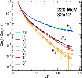
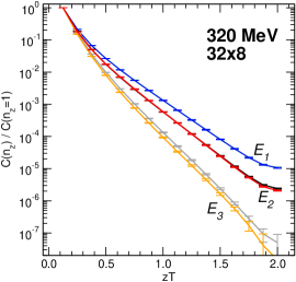
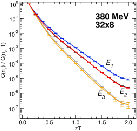
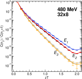
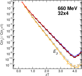
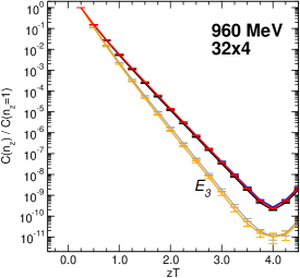
Figure 1: Overview of our spatial correlators in a wide range of temperatures. The correlators are shown as a function of the dimensionless combination $zT=n_{z}/N_{t}$ and are normalized to 1 at $n_{z}=1$. Note that the correlators are for different lattice sizes as indicated (compare Table 3 for details). We label groups of correlators according to the multiplets $E_{1},E_{2}$ and $E_{3}$ as introduced in Eqs. (57) – (59).

The top left panel of Fig. 1 shows correlators at a temperature of $T\sim 220$ MeV, i.e., $1.2\,T_{c}$. All correlation functions of chiral partners are degenerate within errors. In detail, this are the two pairs $(V_{x},A_{x})$ and $(V_{t},A_{t})$, each of which reflects $SU(2)_{R}\times SU(2)_{L}$ symmetry. $U(1)_{A}$ symmetry in the vector channel, represented by the operator pairs $(T_{x},X_{x})$ and $(T_{t},X_{t})$, is manifest for all ensembles. For the scalar $(PS,S)$ pair we find the restoration of $U(1)_{A}$ symmetry to be heavily dependent on the parameters. As it is evident from the top left panel of Fig. 1, $PS$ and $S$ are degenerate within errors for our finest lattice. On the coarser $32\times 8$ ensemble at 220 MeV we find a visible difference of $PS$ and $S$ correlators consistent with previous findings in literature, e.g. the data for staggered quarks presented in Fig. 7 of Ref. Cheng:2010fe .

For temperatures between $T\sim 220$ – $500$ MeV the correlators are grouped into three distinct multiplets:

$$E_{1}: \qquad PS\leftrightarrow S\;,$$ (57)

$$E_{2}: \qquad V_{x}\leftrightarrow T_{t}\leftrightarrow X_{t}\leftrightarrow A_{x}\;,$$ (58)

$$E_{3}: \qquad V_{t}\leftrightarrow T_{x}\leftrightarrow X_{x}\leftrightarrow A_{t}\;.$$ (59)

Possible splittings within each of these multiplets are obviously much smaller than the distances between the multiplets. The multiplet structure reflects the symmetries as follows: The multiplet $E_{1}$ indicates the restoration of $U(1)_{A}$ symmetry. Degeneracies within the multiplets $E_{2}$ and $E_{3}$ reflect the larger symmetries $SU(2)_{CS}$ and $SU(4)$ as discussed in the previous section.

The formation of the multiplet $E_{3}$ is not necessarily a consequence of the $SU(2)_{CS}$ and $SU(4)$ symmetries as the same degeneracy of correlators is seen also for non-interacting quarks (15) and can be attributed to current conservation. Consequently from the observation of the $E_{3}$ multiplet alone we could not claim the emergence of the $SU(2)_{CS}$ and $SU(4)$ symmetries. However, the $E_{2}$ degeneracy is not manifest in the free quark system (15) and indeed can be attributed to the emergent $SU(2)_{CS}$ and $SU(4)$ symmetries.

We speak of separate multiplets when the splittings within the multiplets are much smaller than splittings between different multiplets. All correlators connected by chiral $U(1)_{A}$ and $SU(2)_{L}\times SU(2)_{R}$ transformations are indistinguishable at all temperatures. At temperatures above $T\sim 600$ MeV we observe that the distinct multiplet $E_{2}$, related to emergence of the $SU(2)_{CS}$ and $SU(4)$ symmetries, is washed out. The remaining $E_{3}$ multiplet structure can be attributed to quasi-free quarks.

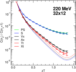
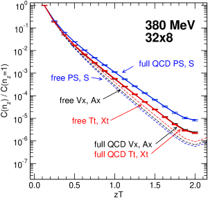
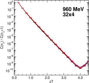
Figure 2: Correlation functions of the bilinears in the $E_{1}$ and $E_{2}$ multiplets. The structure of the plots is the same as described in the caption of Fig. 1, with the addition of the correlators for free quarks shown as dashed lines.

In Fig. 2 we now focus on the $E_{1}$ and $E_{2}$ multiplets at three different temperatures. For comparison we also show the corresponding correlators computed for free quarks (dashed lines). The latter correlators are obtained with the same lattice Dirac operator and lattice size as used for the full QCD but now with a unit gauge configuration. We note that for free quarks only those degeneracies exist that are predicted by the chiral $U(1)_{A}$ and $SU(2)_{L}\times SU(2)_{R}$ symmetries.

For the lowest temperature $T\sim 220$ MeV we still observe a small residual splitting within the $E_{2}$ multiplet, while at $T\sim 380$ MeV the difference nearly vanishes. Furthermore, there is a clear splitting between the $E_{1}$ and $E_{2}$ multiplets indicating $SU(2)_{CS}$ and $SU(4)$ symmetries. In addition all correlators are well separated from their free quark counterparts shown as dashed curves.

At the highest temperature of this study, $T\sim 960$ MeV, the situation has changed considerably: All correlators almost perfectly coincide with the corresponding free correlators, as seen by the dashed lines on top of the data points for the full QCD correlators. Thus at $T\sim 960$ MeV we have reached the region where only chiral $U(1)_{A}$ and $SU(2)_{L}\times SU(2)_{R}$ symmetries exist and the coincidence with the free correlators suggests a gas of quasi-free quarks.

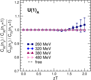
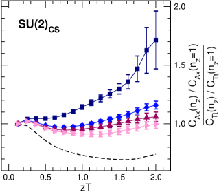
Figure 3: Ratios of normalized correlators for different bilinears from the $E_{2}$ multiplet at different temperatures ($32^{3}\times 8$ lattices): The lhs. plot shows the ratio $C_{X_{t}}/C_{T_{t}}$, i.e., a ratio of correlators connected by $U(1)_{A}$. The rhs. plot shows the ratio $C_{A_{x}}/C_{T_{t}}$, i.e., two correlators connected by $SU(2)_{CS}$ transformations. In both cases we show the corresponding ratios for free quarks as dashed curves.

In an attempt of discussing the observed evolution of symmetries more quantitatively, in Figures 3 and 4 we study ratios of correlators, where the fully symmetric case corresponds to a constant ratio 1 for all $z$. In Fig. 3 we show ratios of normalized correlators for different bilinears from the $E_{2}$ multiplet. The ratios are plotted as function of the dimensionless quantity $zT=n_{z}/N_{t}$ and we compare different temperatures.

In the lhs. plot we show the ratio $C_{X_{t}}/C_{T_{t}}$. The two correlators are related by $U(1)_{A}$ and a deviation from a constant ratio 1 indicates a violation of $U(1)_{A}$. The data shows no breaking effects within errors.

In the rhs. plot we show the ratio $C_{A_{x}}/C_{T_{t}}$. These two correlators are related by $SU(2)_{CS}$ and thus a deviation from 1 indicates a violation of exact $SU(2)_{CS}$. Here the lowest temperature displays sizable residual violation, which gradually becomes smaller with increasing temperature. At $T\sim 380$ MeV the deviation from 1 becomes minimal.

Finally, in Fig. 4 we analyze the $SU(2)_{CS}$ sensitive ratio $C_{A_{x}}/C_{T_{t}}$ for all our ensembles in a wider range of temperatures. We observe an evolution from sizable deviation from 1 at the lowest temperature $T\sim 220$ MeV towards a coincidence with the corresponding ratio of correlators for free quarks at the highest temperature, i.e. $T\sim 960$ MeV. For intermediate temperatures we observe small deviations from 1.

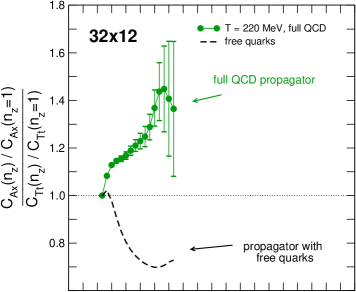
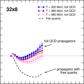
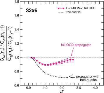
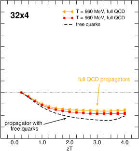
Figure 4: The ratio $C_{A_{x}}/C_{T_{t}}$ for different temperatures. The two correlators from the $E_{2}$ multiplet are related by $SU(2)_{CS}$ and deviations from 1 indicate violation of the symmetry. The 4 different plots group together the results for lattices with the same aspect ratio.

Figs. 3 and 4 demonstrate that – while the chiral symmetries are practically exact – the $SU(2)_{CS}$ symmetry is not exact. Let us introduce a measure for the symmetry breaking and find a temperature range where the symmetry is appropriate.

In general a symmetry is established via its multiplet structure. For any multiplet structure a crucial parameter is the ratio of the splitting within a multiplet to the distance between multiplets. The splitting within a multiplet by itself is irrelevant without a scale, and should be compared to a scale relevant for the given problem, e.g. the distance between multiplets. Consequently, in our case the breaking of $SU(2)_{CS}$ and $SU(4)$ can be identified through the parameter

$$\kappa=\frac{|C_{A_{x}}-C_{T_{t}}|}{|C_{A_{x}}-C_{S}|}.$$ (60)

If $\kappa\ll 1$, then we can declare an approximate or – if zero – an exact symmetry. If $\kappa\sim 1$, the symmetry is absent. The criterion of small $\kappa$ corresponds to the existence of a distinct multiplet $E_{2}$ that should be well separated from the multiplet $E_{1}$. From the free quark expression (15) one finds $\kappa\sim 1$, which stresses again that there is no chiral-spin symmetry for free quarks.

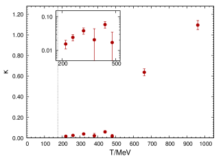
Figure 5: The symmetry breaking parameter $\kappa$ defined in (60) evaluated at $zT=2$ for different temperatures. The dashed line represents $T_{c}$.

In Fig. 5 we show the evolution of the symmetry breaking parameter $\kappa$ as a function of temperature at $zT=2$. The value of $\kappa$ is less than 5 % for all ensembles with $T\sim 220$ – $500$ MeV. This implies that the symmetries that we observe in the range between $T\sim 220$ MeV and $500$ MeV are well pronounced.

At temperatures between $T\sim 500$ MeV and $T\sim 660$ MeV we notice a drastic increase of the symmetry breaking parameter $\kappa$ to values of the order $\sim 1$. We conclude that QCD exhibits an approximate $SU(2)_{CS}$ symmetry in the temperature range between $T\sim 220$ – $500$ MeV ($1.2T_{c}$ – $2.8T_{c}$) with symmetry breaking less than 5% as measured with $\kappa$. This suggests that the $SU(2)_{CS}$ symmetric regime begins just after the $SU(2)_{R}\times SU(2)_{L}$ restoration crossover.

We stress once more that the $SU(2)_{CS}$ symmetry is related to different components of the strong interaction. As we have discussed, an exact $SU(2)_{CS}$ symmetry implies that the interaction is strictly chromo-electric. Thus the observed evolution of the $SU(2)_{CS}$ symmetry as a function of temperature suggests the following picture for the relevant degrees of freedom in high temperature QCD: At $T\sim 220$ MeV we find $C_{A_{x}}/C_{T_{t}}>1$ and a small violation of $SU(2)_{CS}$ such that the interaction between the quarks must be mediated not only by the chromo-electric component, but also to some extent by the chromo-magnetic components of the gluonic field. When increasing the temperature, the ratio $C_{A_{x}}/C_{T_{t}}$ evolves towards 1. This implies that at $T\sim 380$ MeV the chromo-magnetic interaction has become washed out and quarks interact via the chromo-electric field. The remaining small breaking of $SU(2)_{CS}$ is due to the quark kinetic term. It suggests that in this regime the elementary objects are chirally symmetric quarks confined by the chromo-electric field. At even higher temperatures also the contribution of the chromo-electric interaction decreases and the system enters the region of quasi-free quarks, as reflected by the fact that for our highest temperatures the ratio $C_{A_{x}}/C_{T_{t}}$ approaches the corresponding curve for free quarks.

We stress that the emerging $SU(2)_{CS}$ and $SU(4)$ symmetries, observed in the range of $T\sim 220$ MeV to $T\sim 500$ MeV, are incompatible with the picture of free deconfined quarks.

This view is also reflected in the exponential decay properties – i.e., the factors $\propto\exp(-c\,z)$ – of the full QCD correlators. A system of two free quarks cannot have $z$-correlators where the exponent $c$ is smaller than twice the lowest Matsubara frequency $2\omega_{0}$, due to the anti-periodic boundary conditions of fermions in time direction (compare Eq. (16)). If the exponent $c$ is smaller for the interacting case, this suggests that the quark-antiquark system is still coupled into a bosonic compound, since periodic boundary conditions for bosons do allow for the exponent $c$ to be smaller than $2\,\omega_{0}$. Fig. 2 shows that the full $PS$- and $S$-correlators have significantly smaller exponents $c$ than their non-interacting counterparts, which suggests that these correlators correspond to coupled quark-antiquark compounds DeTar:1987xb . In the $J=1$ channels the difference of the exponents $c$ for full and free correlators at temperatures $T<500$ MeV is much smaller, but still visible, and suggests a residual binding also in this case.

VI Conclusions

In this paper we have studied spatial correlators of all possible local $J=0$ and $J=1$ bilinears in high temperature lattice QCD. We use $N_{F}=2$ flavors of domain wall fermions and study temperatures up to $T\sim 960$ MeV. Above the chiral restoration crossover at a pseudo-critical temperature $T_{c}\sim 175$ MeV we observe restoration of chiral $SU(2)_{L}\times SU(2)_{R}$ symmetry for all studied temperatures. While $U(1)_{A}$ symmetry is present in all ensembles above 260 MeV, its restoration at 220 MeV is observed on the finest lattice solely.

In the range between $T\sim 220$ MeV and $T\sim 500$ MeV we observe the formation of multiplets in spatial correlators that indicate larger emergent symmetries described by the chiral spin $SU(2)_{CS}$ and $SU(4)$ groups with the breaking effects below 5 % as measured by $\kappa$. These symmetries include the chiral $U(1)_{A}$ and $SU(2)_{L}\times SU(2)_{R}$ groups as well as transformations that mix the right- and left-handed components of quarks as subgroups. These are not symmetries of the free Dirac action but are symmetries of the fermionic charge. In a given reference frame, which in our case is the medium rest frame, the quark - chromo-electric interaction is invariant under both $SU(2)_{CS}$ and $SU(4)$ transformations, while the quark - chromo-magnetic interaction as well as the quark kinetic term break them.

The emergence of these symmetries in the $T\sim 220$ – $500$ MeV window ($1.2T_{c}$ – $2.8T_{c}$) suggests that the chromo-magnetic interaction between quarks is screened at these temperatures, while the confining chromo-electric interaction is still active. The emergence of approximate $SU(2)_{CS}$ and $SU(4)$ symmetries in the window $T\sim 220$ – $500$ MeV is the principal result of our study. These emergent symmetries are incompatible with the picture of free, deconfined quarks and suggest that the physical degrees of freedom are chirally symmetric quarks bound by the chromo-electric interaction without chromo-magnetic effects. The latter conclusion is based entirely on our lattice observations and the symmetry classification of the QCD Lagrangian, i.e., it is model independent. We remark that correlation functions with the $SU(2)_{CS}$ and $SU(4)$ symmetries cannot be analyzed perturbatively because perturbation theory reflects the symmetries of the free Dirac equation.

While we do not advocate any microscopic description of these ultrarelativistic objects, they are reminiscent of “strings”. A string is the only known mathematical description of purely electric, relativistic objects, though a consistent theory of a relativistic string with quarks at the ends is missing in four dimensions. We refer the $SU(2)_{CS}$ and $SU(4)$ symmetric regime at temperatures $T\sim 220$ – $500$ as the “stringy fluid” to emphasize the possible nature of the objects - chirally symmetric quarks bound by the electric field.

At temperatures above $T\sim 600$ MeV these symmetries disappear and the QCD correlation functions approach the correlators calculated with free, non-interacting quarks. This suggests that only at temperatures $T\sim 1$ GeV and above hot QCD matter can be approximately described as a gas of weakly interacting quarks and gluons – the Quark-Gluon Plasma (QGP).

Our analysis of spatial correlators and their multiplet structure suggests the following three regimes of QCD when increasing the temperature: At low temperatures up to the pseudo-critical temperature $T_{c}$ QCD matter is a hadron gas where all chiral symmetries are broken by the non-zero quark condensate. From the hadron gas regime below $T_{c}$ there is a crossover to a regime with approximate $SU(2)_{CS}$ chiral spin symmetry, where quarks are predominantly bound by the chromo-electric interaction. This crossover coincides or is close to the chiral $SU(2)_{L}\times SU(2)_{R}$ restoration crossover (while in our setup the chiral crossover is at $T_{c}\sim 175$ MeV, for three-flavor QCD the chiral crossover is at a somewhat lower temperature of 155 MeV Bazavov:2018mes ). In the range $T\sim 500$ – $660$ MeV ($2.8T_{c}$ – $3.8T_{c}$) there is a fast increase of symmetry breaking: the confining electric interaction becomes small relative to the quark kinetic term. Finally, up to $T\sim 1$ GeV ($5.7T_{c}$) there is an evolution to a weakly interacting QGP, where the relevant symmetries are the full set of chiral symmetries. Fig. 6 provides an illustrative sketch of this temperature evolution for the effective degrees of freedom of QCD. We note that the temperature range, in which the most drastic changes of thermodynamical bulk quantities occur, coincides qualitatively with the “stringy fluid” regime, see, e.g., Fig. 4 of Ref. Bazavov:2017dsy .

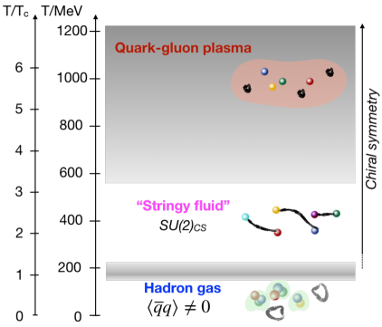
Figure 6: Illustrative sketch for the temperature evolution of the QCD effective degrees of freedom as suggested by the changing symmetry content manifest in our spatial correlators.

Appendix A

All free spatial continuum correlators that we discuss in Section 2 can be expressed as linear combinations of $C_{z}(z)$ and $C_{\tau}(z)$ defined in Eq. (12). These two correlators can be simplified by switching to polar coordinates $p_{x}=r\cos(\varphi)$, $p_{y}=r\sin(\varphi)$. The $\varphi$-integration gives a factor of $2\pi$ and the transformation $\xi^{2}=(r/\omega_{n})^{2}+1$ of the remaining integration variable brings the correlators to the form

$$C_{z}(z) = \frac{1}{2\pi\beta}\sum_{n\in\mathds{Z}}\omega_{n}^{2}\int_{1}^{\infty}\!\!d\xi\,\xi\,e^{\,-2\,z\,|\omega_{n}|\,\xi}\;,$$

$$C_{\tau}(z) = \frac{1}{2\pi\beta}\sum_{n\in\mathds{Z}}\omega_{n}^{2}\int_{1}^{\infty}\!\!d\xi\,\xi\,\frac{1}{\xi^{2}}\,e^{\,-2\,z\,|\omega_{n}|\,\xi}\;.$$ (61)

Both contain the Matsubara sum

$$\sum_{n\in\mathds{Z}}\omega_{n}^{\,2}\;e^{\,-2\,z\,|\omega_{n}|\,\xi} = 2\!\sum_{n\in\mathds{N}_{0}}\!\omega_{n}^{\,2}\;e^{\,-2\,z\,|\omega_{n}|\,\xi}\;=\;\frac{1}{2z^{2}}\frac{d^{2}}{d\xi^{2}}\sum_{n\in\mathds{N}_{0}}e^{\,-2\,z\,|\omega_{n}|\,\xi}$$

$$= \frac{1}{2z^{2}}\frac{d^{2}}{d\xi^{2}}e^{\,-z\,\frac{2\pi}{\beta}\,\xi}\!\!\sum_{n\in\mathds{N}_{0}}\!\!\!\left(\!e^{-2z\frac{2\pi}{\beta}\xi}\!\right)^{\!n}=\frac{1}{2z^{2}}\frac{d^{2}}{d\xi^{2}}\frac{e^{\,-z\,\frac{2\pi}{\beta}\,\xi}}{1\!-\!e^{-2z\frac{2\pi}{\beta}\xi}}=\frac{1}{4z^{2}}\frac{d^{2}}{d\xi^{2}}\frac{1}{\sinh(z\,\frac{2\pi}{\beta}\,\xi)}\;,$$

where in the second step we have split the sum over $n\in\mathds{Z}$ into a positive and a negative part which can be transformed into each other by flipping the sign of $n$ and a trivial shift. Subsequently we generated the factor $\omega_{n}^{\,2}$ with a second derivative and finally used the geometric series formula for the sum. Below we will use both, the final expression as a derivative, as well as the other form of a sum over $n\in\mathds{N}_{0}$.

For solving the first integral $C_{z}(z)$ we use the form of the Matsubara sum (Appendix A) as a second derivative and insert this in (61). Subsequently two partial integrations can be used to solve $C_{z}(z)$ in closed form ($\omega_{0}=\pi/\beta$),

$$C_{z}(z)\,=\,\frac{\pi}{2\beta^{3}}\,\frac{1}{2\,z\omega_{0}}\,\frac{1}{\sinh(2\,z\omega_{0})}\left[\mbox{cotanh}\,(2\,z\omega_{0})+\frac{1}{2\,z\omega_{0}}\right]\;.$$ (63)

For the evaluation of $C_{\tau}(z)$ we keep the sum explicitly and find,

$$C_{\tau}(z)\;=\;\frac{1}{\pi\beta}\sum_{n\in\mathds{N}_{0}}\!\!\omega_{n}^{\,2}\!\int_{2\,z\omega_{n}}^{\infty}\!\!\!\!d\zeta\,\frac{e^{\,-\zeta}}{\zeta}\;=\;\frac{1}{\pi\beta}\sum_{n\in\mathds{N}_{0}}\!\!\omega_{n}^{\,2}\,E_{1}(2\,z\omega_{n})\;.$$ (64)

In the first step we used the variable transformation $\zeta=2\,z\omega_{n}\xi$ which brings the integral into the standard form nist for the exponential integral $E_{1}(x)\equiv\int_{x}^{\infty}d\zeta\,e^{-\zeta}/\zeta$.

We conclude this appendix with quoting the asymptotic forms for the integrals $C_{z}(z)$ and $C_{\tau}(z)$ which can be obtained with power series for standard functions from (63) and the known expansion nist for the exponential integral in (64),

$$C_{z}(z) = \frac{\pi}{\beta^{3}}\,\frac{e^{\,-\,2\,z\omega_{0}}}{2\,z\omega_{0}}\left[1+\frac{1}{2\,z\omega_{0}}\right]\;+\;O\left(\frac{e^{\,-4\,z\omega_{0}}}{z\omega_{0}}\right)\;,$$ (65)

$$C_{\tau}(z) = \frac{\pi}{\beta^{3}}\,\frac{e^{\,-\,2\,z\omega_{0}}}{2\,z\omega_{0}}\left[1-\frac{1}{2\,z\omega_{0}}+O\left(\frac{1}{(z\omega_{0})^{2}}\right)\right]\;+\;O\left(\frac{e^{\,-6\,z\omega_{0}}}{z\omega_{0}}\right).$$

References

- (1) E.V. Shuryak, Phys. Rept. 61, 71 (1980).
- (2) A.M. Polyakov, Phys. Lett. 72B, 477 (1978).
- (3) L.D. McLerran and B. Svetitsky, Phys. Rev. D 24, 450 (1981).
- (4) O. Kaczmarek, F. Karsch, P. Petreczky and F. Zantow, Phys. Lett. B 543, 41 (2002).
- (5) S. Borsanyi, G. Endrodi, Z. Fodor, S.D. Katz and K.K. Szabo, JHEP 1207, 056 (2012).
- (6) P. Petreczky and H.P. Schadler, Phys. Rev. D 92, 094517 (2015).
- (7) F. Karsch, E. Laermann and A. Peikert, Phys. Lett. B 478, 447 (2000).
- (8) A. Bazavov, P. Petreczky and J.H.Weber, Phys. Rev. D 97, 014510 (2018).
- (9) E. V. Shuryak and I. Zahed, Phys. Rev. C 70, 021901 (2004) [hep-ph/0307267].
- (10) C. Ratti, R. Bellwied, M. Cristoforetti and M. Barbaro, Phys. Rev. D 85, 014004 (2012) [arXiv:1109.6243 [hep-ph]].
- (11) S. Mukherjee, P. Petreczky and S. Sharma, Phys. Rev. D 93, no. 1, 014502 (2016) [arXiv:1509.08887 [hep-lat]].
- (12) C.E. DeTar and J.B. Kogut, Phys. Rev. D 36 (1987) 2828.
- (13) K. D. Born et al. [MT(c) Collaboration], Phys. Rev. Lett. 67, 302 (1991).
- (14) J.B. Kogut, J.F. Lagae and D.K. Sinclair, Phys. Rev. D 58, 054504 (1998).
- (15) I. Pushkina et al., Phys. Lett. B 609, 265 (2005).
- (16) W. Florkowski and B.L. Friman, Z. Phys. A 347, 271 (1994).
- (17) S. Wissel, E. Laermann, S. Shcheredin, S. Datta and F. Karsch, PoS LAT 2005, 164 (2006) [hep-lat/0510031].
- (18) R.V. Gavai, S. Gupta and R. Lacaze, PoS LAT2006, 135 (2006), [arXiv:hep-lat/0609074].
- (19) M. Cheng et al., Eur. Phys. J. C 71, 1564 (2011) [arXiv:1010.1216 [hep-lat]].
- (20) D. Banerjee, R. V. Gavai and S. Gupta, Phys. Rev. D 83, 074510 (2011) [arXiv:1102.4465 [hep-lat]].
- (21) B. B. Brandt, A. Francis, H. B. Meyer, O. Philipsen, D. Robaina and H. Wittig, JHEP 1612, 158 (2016) [arXiv:1608.06882 [hep-lat]].
- (22) C. Rohrhofer, Y. Aoki, G. Cossu, H. Fukaya, L. Y. Glozman, S. Hashimoto, C. B. Lang and S. Prelovsek, Phys. Rev. D 96, no. 9, 094501 (2017) Erratum: [Phys. Rev. D 99, no. 3, 039901 (2019)] [arXiv:1707.01881 [hep-lat]].
- (23) G. Cossu et al. [JLQCD Collaboration], Phys. Rev. D 93 (2016) 034507.
- (24) A. Tomiya, G. Cossu, S. Aoki, H. Fukaya, S. Hashimoto, T. Kaneko and J. Noaki, Phys. Rev. D 96, no. 3, 034509 (2017) Addendum: [Phys. Rev. D 96 079902 (2017)].
- (25) G. Cossu, J. Noaki, S. Hashimoto, T. Kaneko, H. Fukaya, P. A. Boyle and J. Doi, arXiv:1311.0084 [hep-lat].
- (26) T. Kaneko et al. [JLQCD Collaboration], PoS LATTICE 2013, 125 (2014) [arXiv:1311.6941 [hep-lat]].
- (27) L.Y. Glozman, Eur. Phys. J. A 51 27 (2015).
- (28) L.Y. Glozman and M. Pak, Phys. Rev. D 92 016001 (2015).
- (29) M. Denissenya, L.Y. Glozman and C.B. Lang, Phys. Rev. D 89 077502 (2014).
- (30) M. Denissenya, L.Y. Glozman and C.B. Lang, Phys. Rev. D 91 034505 (2015).
- (31) M. Denissenya, L.Y. Glozman and M. Pak, Phys. Rev. D 91 114512 (2015). [arXiv:1505.03285 [hep-lat]].
- (32) M. Denissenya, L.Y. Glozman and M. Pak, Phys. Rev. D 92 074508 (2015).
- (33) C.B. Lang and M. Schröck, Phys. Rev. D 84, 087704 (2011).
- (34) L.Y. Glozman, Eur. Phys. J. A 54 117 (2018).
- (35) C. Rohrhofer, Y. Aoki, G. Cossu, L.Y. Glozman, S. Hashimoto and S. Prelovsek, arXiv:1809.00244 [hep-lat].
- (36) A. Bazavov et al., arXiv:1812.08235 [hep-lat].
- (37) F.W.J. Olver, D.W.Lozier, R.F. Boisvert and C.W. Clark, NIST Handbook of Mathematical Functions, Cambridge University Press, New York 2010.