Efficient sliding locomotion with isotropic friction

Abstract

Snakes’ bodies are covered in scales that make it easier to slide in some directions than in others. This frictional anisotropy allows for sliding locomotion with an undulatory gait, one of the most common for snakes. Isotropic friction is a simpler situation (that arises with snake robots for example) but is less understood. In this work we regularize a model for sliding locomotion to allow for static friction. We then propose a robust iterative numerical method to study the efficiency of a wide range of motions under isotropic Coulomb friction. We find that simple undulatory motions give little net locomotion in the isotropic regime. We compute general time-harmonic motions of three-link bodies and find three local optima for efficiency. The top two involve static friction to some extent. We then propose a class of smooth body motions that have similarities to concertina locomotion (including the involvement of static friction) and can achieve optimal efficiency for both isotropic and anisotropic friction.

I Introduction

Snake locomotion has attracted the interest of biologists and engineers for several decades gray1946mechanism ; gray1950kinetics ; jayne1986kinematics ; socha2002kinematics ; HaCh2010b ; MaHu2012a . Many locomoting animals use appendages such as legs, wings, or fins to exert a force on the substrate or surrounding fluid, and propel the rest of the body forward dickinson2000animals . Snakes lack appendages, and thus it is less clear which parts of the snake body should exert propulsive forces, and at which instants during the motion, to move forward efficiently.

A typical way to understand how organisms move is to study physical or computational models and compare their motions with those of the actual organisms dickinson2000animals ; hohenegger2010stability ; olson2011coupling ; lim2012fluid ; jones2016bristles . One can take a step further and pose and solve optimization problems for the models. This can suggest locomotion strategies that are effective for man-made vehicles bar2005biomimetics ; jakimovski2011biologically ; roper2011review . It can also help understand why organisms have evolved in particular ways under a multitude of constraints jacob1977evolution ; alexander1996optima ; langerhans2010ecology .

Often what is optimized is a measure of the efficiency of locomotion. For example, one can maximize the average speed for a given time-averaged power expended by the organism. One can study the effects of physical parameters and constraints by varying them and studying how the optimal solutions change. Well-known examples are optimization studies of organisms moving in low- BeKoSt2003a ; AvGaKe2004a ; TaHo2007a ; fu2007theory ; spagnolie2010optimal ; crowdy2011two ; bittner2018geometrically and high-Reynolds-number fluid flows lighthill1975mathematica ; childress1981mechanics ; sparenberg1994hydrodynamic ; alben2009passive ; michelin2009resonance ; peng2012bb ; gazzola2015gait . For locomotion in frictional (terrestrial or granular) media, frictional forces can result in distinctive modes of efficient (or optimal) locomotion GuMa2008a ; aguilar2016review .

Snakes are limbless reptiles with elongated bodies, supported by a backbone with 100–500 bony segments (vertebrae) lillywhite2014snakes . The vertebrae allow for high flexibility particularly in the lateral (side-to-side) direction, with less flexibility for vertical (dorso-ventral) bending or for torsion. Running along the backbone are muscles that attach to the sides of the vertebrae and cause bending. The snake body is covered in a skin with a compliance (stretchability) greater than that of mammalian skin, and widely variable across species jayne1988mechanical . The outside of the skin is covered in hardened, keratinous scales. Scales on the belly are arranged so that friction is lower when the snake slides towards its head and higher when it slides towards its tail. Muscles attach to scales on the belly and can raise and lower them, modulating their frictional properties and providing a gripping ability seigel1987snakes .

On the basis of experiments and modeling, Hu and Shelley wrote that “snake propulsion on flat ground, and possibly in general, relies critically on the frictional anisotropy of their scales” and measured the friction coefficients for snake specimens sliding in different directions: $\mu_{f}$ (for a snake sliding forward, towards the head), $\mu_{b}$ (sliding backward, towards the tail), and $\mu_{t}$ (sliding transverse to the body axis) HuNiScSh2009a . It is difficult to measure friction coefficients for moving snakes because their direction of motion and friction coefficients usually vary over their bodies. Hu and Shelley found $\mu_{b}\approx 1.3\mu_{f}$ and $\mu_{t}\approx 1.7\mu_{f}$ for corn and milk snakes on cloth HuSh2012a . Marvi and Hu measured forward and backward friction coefficients of corn snakes by placing them on styrofoam inclines and allowing them to slide head-first and tail-first under gravity MaHu2012a . They found $\mu_{b}\approx 1.6\mu_{f}$, and that conscious snakes’ friction coefficients are about twice those of unconscious snakes, which were the focus of previous snake scale friction measurements gray1950kinetics ; HuNiScSh2009a . When conscious, snakes can increase the angles of their scales to grip the surface, increasing friction. Hu and Shelley also studied the motions of snakes wearing cloth sleeves, so that the scales do not contact the substrate, giving a representation of isotropic friction ($\mu_{t}=\mu_{b}=\mu_{f}$). They found that when the snakes undulate while wearing a sleeve, there is little if any forward motion HuNiScSh2009a ; goldman2010wiggling .

Transeth et al. used experiments and simulations to show that for lateral undulation with isotropic friction, locomotion is possible but slow without barriers to push against transeth2008snake ; transeth2009survey . Others have found that snake robots can achieve locomotion with isotropic friction using 3D motions: sinus-lifting (slightly lifting the peaks of the body wave curve off the ground during lateral undulation), sidewinding, inchworm motions, and lateral rolling ohno2001design ; liljeback2012review . Chernousko simulated particular gaits of multilinked bodies with various friction coefficients and found that locomotion could be obtained with isotropic friction chernousko2005modelling . Wagner and Lauga studied the locomotion of a two-mass system moving in one dimension with isotropic friction (equal in the forward and backward directions) and found that locomotion is possible if the two masses have different friction coefficients and the length of the link connecting them has an asymmetric stroke cycle wagner2013crawling . For the swimming of microorganisms in a viscous fluid (at zero Reynolds number), the drag anisotropy of long slender bodies and appendages is known to be essential for locomotion lauga2009hydrodynamics .

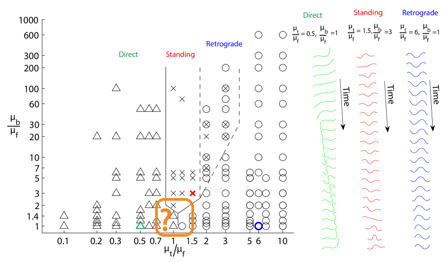
Figure 1: Left: Classification of local optima across friction coefficient space, computed in AlbenSnake2013 . Right: Three sequences of snapshots of locally optimal motions giving examples of direct, standing, and retrograde waves. These occur at particular friction coefficient ratios, listed above the snapshots and marked with green, red, and blue symbols in the panel at left. The three sequences of snapshots are given over one period of motion, and displaced vertically to enhance visibility but with the actual horizontal displacement.

In a previous theoretical/computational study we optimized smooth snake body kinematics for efficiency, starting from random initial ensembles AlbenSnake2013 . The kinematics were described by the coefficients of a double series, Fourier in time (with unit period) and Chebyshev (polynomials) in arc length along the body axis, truncated at 45 modes (9 temporal by 5 spatial) and in some cases 190 modes (19 temporal by 10 spatial). The searches were begun at random points in the 45- and 190-dimensional spaces of these coefficients. We searched for smooth time-periodic body kinematics that maximize a definition of efficiency—the net distance traveled in one period divided by the work done against friction in one period AlbenSnake2013 . The optimizers were calculated and classified as shown in figure 1, across the space of $\mu_{t}/\mu_{f}$ (horizontal axis) and $\mu_{b}/\mu_{f}$ (vertical axis). Many of the local optima could be classified as retrograde traveling waves—waves of curvature moving opposite to the body’s direction of motion (i.e. lateral undulation)—prevalent for $\mu_{t}/\mu_{f}\gtrsim 6$; symmetric standing waves, observed for $\mu_{b}/\mu_{f}\geq 2$ and $0.7<\mu_{t}/\mu_{f}\leq 3$; or direct waves—waves of curvature moving with the body’s direction of motion—observed for $\mu_{t}/\mu_{f}\lesssim 0.7$. Direct waves have also been observed in the undulatory swimming of polychaete worms, with appendages extending perpendicular to the body axis taylor1952analysis ; sfakiotakis2009undulatory . Examples of these three classes of optima are shown in the snapshots on the right side of figure 1. In this study, one possible local optimum was observed with isotropic friction $\mu_{b}/\mu_{f}=\mu_{t}/\mu_{f}=1$, but the efficiency gradient norm was only reduced by about two orders of magnitude from the random initial kinematics AlbenSnake2013 . Usually computations did not converge to local optima in the vicinity of isotropic friction (orange box in figure 1). Because isotropic friction is common for snake robots (e.g. without scales) liljeback2012review , is close to the measured friction coefficients for real snakes HuSh2012a , and is physically the simplest situation, a better understanding of planar locomotion in this regime is useful. Isotropic friction is also a model of situations where snake scales are less effective—e.g. on loose, sandy, or slippery terrain maladen2011undulatory . Effective kinematics for planar locomotion with isotropic friction is the main topic of this study.

II Model

We use the same Coulomb-friction snake model as HuNiScSh2009a ; HuSh2012a ; JiAl2013 and other recent works. The snake body is thin compared to its length, so for simplicity we approximate its motion by that of a planar curve $\mathbf{X}(s,t)=(x(s,t),y(s,t))$, parametrized by arc length $s$ and varying with time $t$. Schematic diagrams are shown in figure 2.

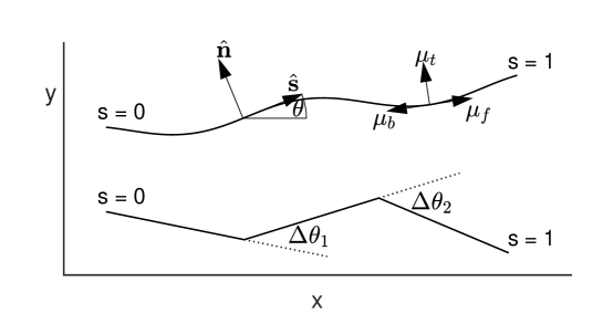
Figure 2: Schematic diagrams of model snakes. Top: a smooth planar curve parametrized by arc length $s$ (nondimensionalized by snake length), at an instant in time. The tangent angle and the unit vectors tangent and normal to the curve at a point are labeled. Vectors representing forward, backward and transverse velocities are shown with the corresponding friction coefficients $\mu_{f}$, $\mu_{b}$, and $\mu_{t}$. Bottom: a three-link snake with changes in angles $\Delta\theta_{1}$ (here positive) and $\Delta\theta_{2}$ (here negative) between the links.

The tangent angle is denoted $\theta(s,t)$ and satisfies $\partial_{s}x=\cos\theta$ and $\partial_{s}y=\sin\theta$. The unit vectors tangent and normal to the curve are $\hat{\mathbf{s}}=(\partial_{s}x,\partial_{s}y)$ and $\hat{\mathbf{n}}=(-\partial_{s}y,\partial_{s}x)$ respectively. The basic problem is to prescribe the time-dependent shape of the snake in order to obtain efficient locomotion. We consider both smooth bodies (figure 2, top), and three-link bodies (figure 2, bottom). The latter are described by $\Delta\theta_{1}$ and $\Delta\theta_{2}$, the differences between the tangent angles of the adjacent links.

We prescribe the body shape as $\Theta(s,t)$, the tangent angle in the “body frame,” defined as a frame that rotates and translates so that at every time the body tail ($s=0$) lies at the origin in the body frame and the body has zero tangent angle at the tail ($\Theta(0,t)=0$). In the three-link case, $\Theta(s,t)=\Delta\theta_{1}(t)H(s-1/3)+\Delta\theta_{2}(t)H(s-2/3)$, where $H$ is the Heaviside function. For all bodies (smooth and three-link), the tangent angle in the physical (or lab) frame is obtained by adding $\theta_{0}(t)$, the actual tangent angle at the tail, to $\Theta(s,t)$:

$$\theta(s,t) =\theta_{0}(t)+\Theta(s,t).$$ (1)

The body position in the lab frame is then obtained by integration:

$$x(s,t) =x_{0}(t)+\int_{0}^{s}\cos\theta(s^{\prime},t)ds^{\prime},$$ (2)

$$y(s,t) =y_{0}(t)+\int_{0}^{s}\sin\theta(s^{\prime},t)ds^{\prime}.$$ (3)

The tail position $(x_{0}(t),y_{0}(t))$ and tangent angle $\theta_{0}(t)$ (or equivalently, $\dot{x}_{0}(t),\dot{y}_{0}(t)$, and $\dot{\theta}_{0}(t)$) are determined by the force and torque balance for the snake, i.e. Newton’s second law:

$$\int_{0}^{L}\rho\partial_{tt}xds =\int_{0}^{L}f_{x}ds,$$ (4)

$$\int_{0}^{L}\rho\partial_{tt}yds =\int_{0}^{L}f_{y}ds,$$ (5)

$$\int_{0}^{L}\rho\mathbf{X}^{\perp}\cdot\partial_{tt}\mathbf{X}ds =\int_{0}^{L}\mathbf{X}^{\perp}\cdot\mathbf{f}ds.$$ (6)

Here $L$ is the body length, $\rho$ is the body’s mass per unit length, and $\mathbf{X}^{\perp}=(-y,x)$. For simplicity, the body is assumed to be locally inextensible so $L$ is constant in time. $\mathbf{f}$ is the force per unit length on the snake due to Coulomb friction with the ground:

$$\mathbf{f}(s,t) =-\rho g\mu_{t}\left(\widehat{\partial_{t}{\mathbf{X}}}\cdot\hat{\mathbf{n}}\right)\hat{\mathbf{n}}-\rho g\left(\mu_{f}H\left(\widehat{\partial_{t}{\mathbf{X}}}\cdot\hat{\mathbf{s}}\right)+\mu_{b}\left(1-H\left(\widehat{\partial_{t}{\mathbf{X}}}\cdot\hat{\mathbf{s}}\right)\right)\right)\left(\widehat{\partial_{t}{\mathbf{X}}}\cdot\hat{\mathbf{s}}\right)\hat{\mathbf{s}}.$$ (7)

Again $H$ is the Heaviside function and the hats denote normalized vectors. When $\|\partial_{t}{\mathbf{X}}\|=0$ we define $\widehat{\partial_{t}{\mathbf{X}}}$ to be $\mathbf{0}$. According to (7) the snake experiences friction with different coefficients for motions in different directions. The frictional coefficients are $\mu_{f}$, $\mu_{b}$, and $\mu_{t}$ for motions in the forward ($\hat{\mathbf{s}}$), backward ($-\hat{\mathbf{s}}$), and transverse (i.e. normal, $\pm\hat{\mathbf{n}}$) directions, respectively. In general the snake velocity at a given point has both tangential and normal components, and the frictional force density has components acting in each direction. A similar decomposition of force into directional components occurs for viscous fluid forces on slender bodies cox1970motion .

We assume that the body shape $\Theta(s,t)$ is periodic in time with period $T$, similar to the steady locomotion of real snakes HuNiScSh2009a . We nondimensionalize equations (4)–(6) by dividing lengths by the snake length $L$, time by $T$, and mass by $\rho L$. Dividing both sides by $g$ we obtain:

$$\frac{L}{gT^{2}}\int_{0}^{1}\partial_{tt}xds =\int_{0}^{1}f_{x}ds,$$ (8)

$$\frac{L}{gT^{2}}\int_{0}^{1}\partial_{tt}yds =\int_{0}^{1}f_{y}ds,$$ (9)

$$\frac{L}{gT^{2}}\int_{0}^{1}\mathbf{X}^{\perp}\cdot\partial_{tt}\mathbf{X}ds =\int_{0}^{1}\mathbf{X}^{\perp}\cdot\mathbf{f}ds.$$ (10)

In (8)–(10) and from now on, all variables are dimensionless. If the body accelerations are not very large, as is often the case for robotic and real snakes HuNiScSh2009a , $L/gT^{2}\ll 1$, which means that the body’s inertia is negligible. By setting inertia—and the left hand sides of (8)–(10)—to zero, we simplify the equations considerably:

$$\int_{0}^{1}f_{x}ds =\int_{0}^{1}f_{y}ds=\int_{0}^{1}\mathbf{X}^{\perp}\cdot\mathbf{f}ds=0.$$ (11)

In (11), the dimensionless force $\mathbf{f}$ is

$$\mathbf{f}(s,t)=-\mu_{t}\left(\widehat{\partial_{t}{\mathbf{X}}}\cdot\hat{\mathbf{n}}\right)\hat{\mathbf{n}}-\left(\mu_{f}H(\widehat{\partial_{t}{\mathbf{X}}}\cdot\hat{\mathbf{s}})+\mu_{b}(1-H(\widehat{\partial_{t}{\mathbf{X}}}\cdot\hat{\mathbf{s}}))\right)\left(\widehat{\partial_{t}{\mathbf{X}}}\cdot\hat{\mathbf{s}}\right)\hat{\mathbf{s}}.$$ (12)

Similar models were used in GuMa2008a ; HuNiScSh2009a ; HuSh2012a ; JiAl2013 ; AlbenSnake2013 ; wang2014optimizing ; wang2018dynamics , and the same model was found to agree well with the motions of biological snakes in HuNiScSh2009a .

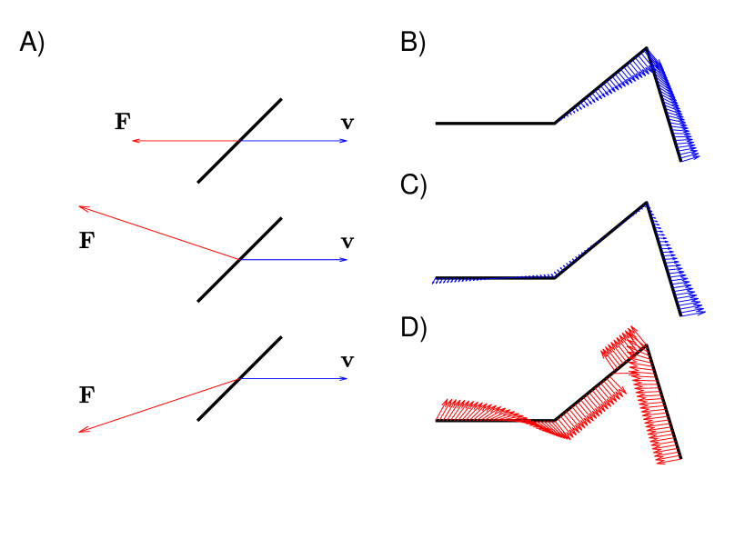
Figure 3: A) Frictional force $\mathbf{F}$ (red vector) acting on a flat plate moving uniformly with horizontal velocity $\mathbf{v}$ (blue vector) when the transverse friction coefficient $\mu_{t}$ is equal to (top), greater than (middle), or less than (bottom) the forward friction coefficient $\mu_{f}$. B) Velocity distribution (blue vectors) on a three-link body with zero translational and rotational velocities ($\dot{\mathbf{X}}_{0}$ and $\dot{\theta}_{0}$) at the tail (left endpoint). Here $\Delta\theta_{1}$ = 39 degrees, $\Delta\theta_{2}$ = -113 degrees, $\dot{\Delta\theta}_{1}$ = -0.56, and $\dot{\Delta\theta}_{2}=1$. C) Velocity distribution in the lab frame: the translational and rotational velocities at the tail are such that the integrated force and torque due to the frictional force distributions (red vectors shown in panel D) are zero.

Figure 3 shows examples of the force-velocity relationship expressed by (12). Panel A shows the total frictional force $\mathbf{F}$ (red vector) on a flat plate with a 45-degree tangent angle and uniform horizontal velocity $\mathbf{v}$ (blue vector) for three different choices of friction coefficients. At the top is isotropic friction, $\mu_{f}=\mu_{t}=1$ ($\mu_{b}$ is not involved here since $\mathbf{v}\cdot\hat{\mathbf{s}}>0$). With isotropic friction, $\mathbf{f}$ is directed opposite to $\mathbf{v}$. The middle case has $\mu_{f}=1$ and $\mu_{t}=2$, increasing the force component in the $\hat{\mathbf{n}}$-direction. The bottom case has instead $\mu_{f}=2$ and $\mu_{t}=1$, increasing the force component in the -$\hat{\mathbf{s}}$-direction. Panel B shows an example of a motion of a three-link body where the tail velocities $\dot{x}_{0}(t),\dot{y}_{0}(t)$, and $\dot{\theta}_{0}(t)$ are zero. Here $\Delta\theta_{1}$ is decreasing and $\Delta\theta_{2}$ is increasing in time, resulting in the nonuniform velocity distribution (piecewise linear in $s$) shown by the blue vectors. The force and torque balance equations are not satisfied by this motion. Panel C shows the same motion but with $\dot{x}_{0}(t),\dot{y}_{0}(t)$, and $\dot{\theta}_{0}(t)$ chosen to satisfy equations (11). This adds a counterclockwise rotation and downward and leftward translation to the body. The resulting force distribution is shown by the red vectors in panel D. The net force and torque from this distribution are zero. Although the velocities are small on the first two links, the forces are large—the normalization of velocities in (12) means that small velocities can give rise to $O$(1) forces. The motion in panel C is approximately one in which only the third link is moving, rotating counterclockwise, but the small but nonzero velocities on the first two links are enough to give forces and torques that balance those on the third link.

Instead of solving (11) for $\{{x}_{0}(t),{y}_{0}(t),{\theta}_{0}(t)\}$ directly, we solve them for $\{\dot{x}_{0}(t),\dot{y}_{0}(t),\dot{\theta}_{0}(t)\}$, which can be done (mostly) in parallel, speeding up the computations. We take time derivatives of (1)-(3), using vector notation for position:

$$\partial_{t}\theta(s,t) =\dot{\theta}_{0}(t)+\partial_{t}\Theta(s,t).$$ (13)

$$\partial_{t}\mathbf{X}(s,t) =\dot{\mathbf{X}}_{0}(t)+\int_{0}^{s}\left(\dot{\theta}_{0}(t)+\partial_{t}\Theta(s,t)\right)\hat{\mathbf{n}}ds^{\prime}.$$ (14)

Given $\Theta(s,t)$ and $\partial_{t}\Theta(s,t)$, we first solve (11) with $\theta_{0}(t)=0$ and $\mathbf{X}_{0}(t)=0$ to obtain a solution $\{\dot{\mathbf{X}}_{0b}(t),\dot{\theta}_{0b}(t)\}$ in the body frame for the unknowns $\{\dot{\mathbf{X}}_{0}(t),\dot{\theta}_{0}(t)\}$ in (13)-(14). The solution $\{\dot{\mathbf{X}}_{0b}(t),\dot{\theta}_{0b}(t)\}$ represents the tail velocity if the body is rotated by $-\theta_{0}(t)$ so that the tail has zero tangent angle. The position $\mathbf{X}$ and tangent and normal vectors $\hat{\mathbf{s}},\hat{\mathbf{n}}$ in the lab frame are simply those in the body frame rotated by $\theta_{0}(t)$. If we set $\dot{\theta}_{0}(t)=\dot{\theta}_{0b}(t)$ and let $\dot{\mathbf{X}}_{0}(t)$ be $\dot{\mathbf{X}}_{0b}(t)$ rotated by $\theta_{0}(t)$, then we find that the lab frame velocity $\partial_{t}{\mathbf{X}}$ in (14) is the body frame velocity rotated by $\theta_{0}(t)$. Hence $\mathbf{f}$ in (12) is that in the body frame rotated by $\theta_{0}(t)$ and $\mathbf{X}^{\perp}\cdot\mathbf{f}$ is unchanged (this dot product and those in $\mathbf{f}$ are unchanged by the rotation)—so both $\mathbf{f}$ and $\mathbf{X}^{\perp}\cdot\mathbf{f}$ still integrate to zero under the transformation from the body to lab frame. To summarize: if $\{\dot{\mathbf{X}}_{0b}(t),\dot{\theta}_{0b}(t)\}$ solve (11) with $\{\mathbf{X}_{0}(t),{\theta}_{0}(t)\}$ equal to zero (i.e. in the body frame), then $\dot{\mathbf{X}}_{0}(t)=\mathbf{R}_{\theta_{0}(t)}\dot{\mathbf{X}}_{0b}(t)$ and $\dot{\theta}_{0}(t)=\dot{\theta}_{0b}(t)$ solve (11) with general $\{\mathbf{X}_{0}(t),{\theta}_{0}(t)\}$, when the body is also rotated by $\theta_{0}(t)$ (i.e. the body is in the lab frame). Here

$$\mathbf{R}_{\theta_{0}(t)}=\begin{pmatrix}\cos\theta_{0}(t)&\hfill-\sin\theta_{0}(t)\cr\sin\theta_{0}(t)&\hfill\cos\theta_{0}(t)\end{pmatrix},$$ (15)

the matrix that rotates by $\theta_{0}(t)$.

We can solve for $\{\dot{\mathbf{X}}_{0b}(t),\dot{\theta}_{0b}(t)\}$ at all time steps in parallel, since only $\Theta(s,t)$ and $\partial_{t}\Theta(s,t)$ are required. Then we integrate $\dot{\theta}_{0}(t)=\dot{\theta}_{0b}(t)$ forward in time to obtain the tail tangent angle starting from $\theta_{0}(0)=0$ (an arbitrary constant that sets the overall trajectory direction). Then we integrate $\dot{\mathbf{X}}_{0}(t)=\mathbf{R}_{\theta_{0}(t)}\dot{\mathbf{X}}_{0b}(t)$ forward in time starting from $\mathbf{X}_{0}(0)=0$ (another arbitrary constant) to obtain the tail position in time. Then the complete body motion is known from (1)-(3).

In this work we will consider only motions that involve zero net rotation over one period, i.e. $\theta_{0}(1)=\theta_{0}(0)$. Then the motion after one period is a pure translation, with all points on the body moving the same distance

$$d=\sqrt{\left(x_{0}(1)-x_{0}(0)\right)^{2}+\left(y_{0}(1)-y_{0}(0)\right)^{2}}.$$ (16)

The work done by the snake against friction over one period is

$$W =\int_{0}^{1}\int_{0}^{1}-\mathbf{f}(s,t)\cdot\partial_{t}\mathbf{X}(s,t)\,ds\,dt.$$ (17)

When the body shape motion $\Theta(s,t)$ is uniformly sped up or slowed down—i.e. when

$$\Theta(s,t)\rightarrow\Theta(s,ct),\quad\partial_{t}\Theta(s,t)\rightarrow c\partial_{t}\Theta(s,ct)$$ (18)

for some constant $c>0$, then the force and torque balance equations are satisfied when the tail motion undergoes the same scaling:

$$\{x_{0}(t),y_{0}(t),\theta_{0}(t)\}\rightarrow\{{x}_{0}(ct),{y}_{0}(ct),{\theta}_{0}(ct)\},\quad\{\dot{x}_{0}(t),\dot{y}_{0}(t),\dot{\theta}_{0}(t)\}\rightarrow c\{\dot{x}_{0}(ct),\dot{y}_{0}(ct),\dot{\theta}_{0}(ct)\}$$ (19)

and so does the overall body motion:

$$\mathbf{X}(s,t)\rightarrow\mathbf{X}(s,ct),\quad\partial_{t}\mathbf{X}(s,t)\rightarrow c\partial_{t}\mathbf{X}(s,ct).$$ (20)

We can see this by first plugging the transformed quantities into (13)-(14), to verify that those equations are still obeyed. We also have $\widehat{\partial_{t}{\mathbf{X}}}(s,t)\rightarrow\widehat{\partial_{t}{\mathbf{X}}}(s,ct)$, and so the frictional force $\mathbf{f}(s,t)\rightarrow\mathbf{f}(s,ct)$ by (12), assuming $c>0$ (note that $\hat{\mathbf{s}}(s,t)\rightarrow\hat{\mathbf{s}}(s,ct)$ and $\hat{\mathbf{n}}(s,t)\rightarrow\hat{\mathbf{n}}(s,ct)$) and the torque density $\mathbf{X}^{\perp}\cdot\mathbf{f}$ has the same transformation. If $\mu_{b}=\mu_{f}$ then the $H(\widehat{\partial_{t}{\mathbf{X}}}\cdot\hat{\mathbf{s}})$ term drops out of $\mathbf{f}$ in (12) and the same scaling holds for $c<0$ also ($\mathbf{f}$ changes sign uniformly in this case). If instead $\mu_{b}\neq\mu_{f}$, then the solutions are not simply time-reversed when the shape change is time-reversed.

Imagine now that we take a given periodic motion and repeat it $n$ times in a period. Then the velocities are multiplied by $n$, and so is the net distance $d$. The same is true of $W$ since in (17), $\partial_{t}\mathbf{X}(s,t)\rightarrow n\partial_{t}\mathbf{X}(s,nt)$ and $\mathbf{f}$ is unchanged. Since $d$ and $W$ both scale with the speed of the motion, it makes sense to define an efficiency as

$$\lambda=\frac{d}{W}.$$ (21)

which is the same when a given motion is sped up or slowed down. A somewhat more general problem, not pursued here, is to find motions that maximize $d$ for a given $W>0$, and then vary $W$. For small $W$, only a limited set of periodic motions—those with small amplitude—can perform work $W$ in a period. When $W$ is large, large-amplitude motions can perform work $W$, but also small amplitude motions by repeating the motion a given number of times. Hence as $W$ becomes larger we consider a larger class of motions that can eventually approximate essentially any periodic motion.

Next we will calculate $W$, $d$, and $\lambda$ for certain examples of motions (i.e. $\Theta(s,t)$) with both isotropic ($\mu_{f}=\mu_{t}=\mu_{b}=1$) and anisotropic friction. Then we will focus on the isotropic case. We will examine the class of time-harmonic three-link motions and then propose a class of smooth motions that optimize $\lambda$.

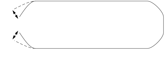
Figure 4: Sketch of a body motion for which the kinetic friction model has no solution, so a model of static friction is used.

Equations (11) assume only kinetic friction is involved, but in reality there is also static friction. In figure 4 we show an example of a motion for which the kinetic friction model has no solution. That is, for the $\Theta(s,t)$ corresponding to this motion (not given mathematically here), no choice of $\{\dot{x}_{0}(t),\dot{y}_{0}(t),\dot{\theta}_{0}(t)\}$ can solve equations (11). Initially the body is given by the solid line. The two flaps on the left side oscillate periodically, sweeping out a region shown by arrows between the solid line and the dashed lines. On the upstroke, the combined vertical force and torque on the flaps from kinetic friction (12) is zero by symmetry, but there is a net horizontal force to the right. If we assume isotropic friction, the horizontal force per unit length on the flaps from (12) lies between 0 and 1, since the flaps move leftward and upward. The rest of the body cannot balance this force exactly for the following reasons. Its motion can only be horizontal to maintain vertical force balance. Therefore, by (12) it has horizontal force per unit length -1, 0, or +1, and a much larger length than the flaps. None of these choices gives zero net horizontal force on the body as a whole. The problem is resolved physically by including static friction: a force density between 0 and that given by kinetic friction when the velocity is zero bhushan2013introduction . Further examples will be given (for three-link bodies) in section V (e.g. figure 10).

To allow for static friction, we use a simple modification of (12) involving a regularization parameter $\delta$:

$$\mathbf{f}_{\delta}(s,t) \equiv-\mu_{t}\left(\widehat{\partial_{t}{\mathbf{X}}}_{\delta}\cdot\hat{\mathbf{n}}\right)\hat{\mathbf{n}}-\left(\mu_{f}H(\widehat{\partial_{t}{\mathbf{X}}}_{\delta}\cdot\hat{\mathbf{s}})+\mu_{b}(1-H(\widehat{\partial_{t}{\mathbf{X}}}_{\delta}\cdot\hat{\mathbf{s}}))\right)\left(\widehat{\partial_{t}{\mathbf{X}}}_{\delta}\cdot\hat{\mathbf{s}}\right)\hat{\mathbf{s}},$$ (22)

$$\widehat{\partial_{t}{\mathbf{X}}}_{\delta} \equiv\frac{\left(\partial_{t}x,\partial_{t}y\right)}{\sqrt{\partial_{t}x^{2}+\partial_{t}y^{2}+\delta^{2}}}.$$ (23)

Here $\delta$ is small, $10^{-4}$ in our computations. We find empirically that there is little change in the results (less than 1% in relative magnitude) for $\delta$ in the range $(0,10^{-4}]$. When $\sqrt{\partial_{t}x^{2}+\partial_{t}y^{2}}$ is similar in magnitude to $\delta$, the force density in (22) varies between 0 and 1 in magnitude, times the appropriate friction coefficient. Therefore we obtain the full range of force densities when velocities are very small, which approximates static friction. In addition to their simplicity, we find empirically that expressions (22)-(23) have desirable properties including the existence of unique solutions using the numerical algorithm described next. More specifically, for all motions shown in the work, our iterative numerical method (described next) finds a unique solution $\{\dot{x}_{0}(t),\dot{y}_{0}(t),\dot{\theta}_{0}(t)\}$ to equations (11) with $\mathbf{f}_{\delta}$ in place of $\mathbf{f}$, for a large number of initial guesses (covering a wide range including choices very far from the solution). Similar types of Coulomb friction regularization (sometimes involving the arctangent function) have been used for many years in dynamical simulations involving friction popov2010contact ; pennestri2016review . In our case, $\delta$ needs to be small compared to any physical velocities we wish to resolve. In particular, $\delta$ should be small compared to the speed of body deformations: the typical magnitude of $\partial_{t}\Theta(s,t)$ multiplied by the range of arc length in which it varies from zero.

III Numerical method

In previous work AlbenSnake2013 , we computed solutions to equations (11) using quasi-Newton methods. Two major challenges of such methods are finding an initial guess that is sufficiently close for convergence, and choosing a step size in the line search that moves the solution towards convergence. The components of $\mathbf{f}_{\delta}$ behave like smoothed step functions near zero velocity. If the solution has velocities near zero (i.e. involves static friction), Newton’s method requires a very good initial guess, within $O(\delta)$ of the solution, to converge. The behavior is similar to that for the arctangent function, a classic example used to illustrate the limited basin of attraction for Newton’s method near a root kelley1995iterative ; dennis1996numerical .

To compute large numbers of solutions to (11) in parallel, we have developed a more robust iterative scheme that converges with any initial guess (for all cases studied, a large number including those in this work) and does not require a line search. The iteration is a fixed point iteration using a linearization of the regularized version of equations (11). At time $t$, given $\Theta(s,t)$ and a guess $\{\dot{x}^{n}_{0}(t),\dot{y}^{n}_{0}(t),\dot{\theta}^{n}_{0}(t)\}$, we use (13)-(14) to compute the corresponding $\{\partial_{t}{x}^{n}(s,t),\partial_{t}{y}^{n}(s,t),\partial_{t}{\theta}^{n}(s,t)\}$, and then solve

$$\int_{0}^{1}\tilde{f}_{\delta x}ds =\int_{0}^{1}\tilde{f}_{\delta y}ds=\int_{0}^{1}\mathbf{X}^{\perp}\cdot\tilde{\mathbf{f}}_{\delta}ds=0$$ (24)

for a new iterate $\{\dot{x}^{n+1}_{0}(t),\dot{y}^{n+1}_{0}(t),\dot{\theta}^{n+1}_{0}(t)\}$ where

$$\tilde{\mathbf{f}}_{\delta}(s,t) \equiv-\mu_{t}\left(\tilde{\widehat{\partial_{t}{\mathbf{X}}}}_{\delta}\cdot\hat{\mathbf{n}}\right)\hat{\mathbf{n}}-\left(\mu_{f}H(\tilde{\widehat{\partial_{t}{\mathbf{X}}}}_{\delta}\cdot\hat{\mathbf{s}})+\mu_{b}(1-H(\tilde{\widehat{\partial_{t}{\mathbf{X}}}}_{\delta}\cdot\hat{\mathbf{s}}))\right)\left(\tilde{\widehat{\partial_{t}{\mathbf{X}}}}_{\delta}\cdot\hat{\mathbf{s}}\right)\hat{\mathbf{s}},$$ (25)

$$\tilde{\widehat{\partial_{t}{\mathbf{X}}}}_{\delta} \equiv\frac{\left(\partial_{t}x^{n+1},\partial_{t}y^{n+1}\right)}{\sqrt{\left(\partial_{t}x^{n}\right)^{2}+\left(\partial_{t}y^{n}\right)^{2}+\delta^{2}}}.$$ (26)

Iterate $n$ is used in the denominator of (26), so the new iterate $\{\dot{x}^{n+1}_{0}(t),\dot{y}^{n+1}_{0}(t),\dot{\theta}^{n+1}_{0}(t)\}$ appears only in the numerator, and (24)-(26) depend linearly on it (in the body frame, where $\mathbf{X},\hat{\mathbf{s}}$, and $\hat{\mathbf{n}}$ are known). Hence we obtain the new iterate $\{\dot{x}^{n+1}_{0}(t),\dot{y}^{n+1}_{0}(t),\dot{\theta}^{n+1}_{0}(t)\}$ by solving 3-by-3 linear systems at each $t$ (decoupled when solving in the body frame). We observe empirically that this approach sacrifices the quadratic or superlinear convergence of Newton-type methods for linear (geometric) convergence. In almost all cases the convergence is quite fast, however. There are a small number of cases involving static friction where the rate of geometric convergence is slower. However these cases are sufficiently few that even with more iterates, the cost of obtaining convergence is small. The loss of superlinear convergence is relatively modest compared to the increased simplicity and robustness of the algorithm.

IV Examples of motions

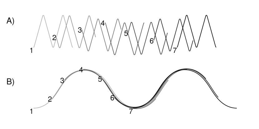
Figure 5: Snapshots of the snake body when executing time-periodic traveling wave body deformations (over one time period, darker at later times, labeled near the tail in numerical order). Top: Rightward-moving smoothed triangular deformation wave. Since $\mu_{t}=1\ll 100=\mu_{f}$, the body moves rightward (i.e. a direct wave). The body tangent angle is $\approx\pm 1.3$ in the straight regions ($\Theta(s,t)=1.3\tanh(20\sin(2\pi(2s-t)))$). Bottom: Leftward-moving sinusoidal deformation wave with wavelength 1 ($\Theta(s,t)=\sin(2\pi(s+t))$). Since $\mu_{f}=1\ll 100=\mu_{t}$, the body moves rightward (i.e. a retrograde wave).

We now present numerical solutions of the model described in section II. We show motions that are approximately optimal with very anisotropic friction, and then show how these motions perform with isotropic friction.

In figure 5A we show snapshots of the body when executing a rightward-moving smoothed triangular wave ($\Theta(s,t)=1.3\tanh(20\sin(2\pi(2s-t)))$) with friction much smaller in the transverse direction than in the tangential direction ($\mu_{t}=1\ll 100=\mu_{f}=\mu_{b}$). The motion is almost entirely in the transverse direction, and due to the almost vertical body slope, the transverse direction is approximately horizontal, close to the direction of locomotion. Consequently the efficiency $\lambda$ is close to 1 (0.93 here). With slight modifications to the motion, efficiency can be made to approach 1. Efficiency increases as the deformation wavelength decreases, so that zero net vertical force and torque are obtained with a purely horizontal motion, decreasing wasted vertical motion that is not in the direction of locomotion. Efficiency also increases as the deformation wave is made steeper (body tangent angle approaches $\pm\pi/2$), so transverse motion is aligned with the direction of locomotion. In this limit the body motion is purely transverse and purely in the direction of motion. Since $\mu_{t}=1$, the work done per unit distance traveled tends to 1.

Figure 5B shows snapshots when the anisotropy is reversed ($\mu_{f}=1\ll 100=\mu_{t}$), so friction is much smaller in the tangential direction (similar to snake robots with wheels whose axes are transverse to the body axis hopkins2009survey ). Here $\mu_{b}=1$ but is arbitrary since there is no backward motion. The body deforms as a sinusoidal leftward moving wave ($\Theta(s,t)=\sin(2\pi(s+t))$). The efficiency $\lambda$ is 0.76, and can be made to approach 1 in the limit $\mu_{t}\to\infty$ by decreasing the amplitude and the deformation wavelength, so motion is almost purely in the tangential direction and in the direction of motion. Since $\mu_{f}=1$, the work done per unit distance traveled tends to 1. Unlike in panel A, here the wave shape (whether sinusoidal, triangular, etc.) does not matter in the limiting case of optimal efficiency. The motions in 5A and B are somewhat idealized versions of the direct and retrograde waves shown in figure 1 and are discussed in AlbenSnake2013 . With large backward friction, and $\mu_{f}\approx\mu_{t}\approx 1$ ratcheting motions were found to be locally optimal in that work. Now we show that with isotropic friction, none of these motions is effective.

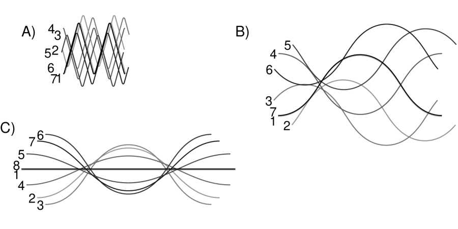
Figure 6: Snapshots of the snake body over one time period (darker at later times, labeled near the tail in numerical order) when executing time-periodic body deformations with isotropic friction ($\mu_{t}$ = $\mu_{f}$ = $\mu_{b}$ = 1). A) Traveling wave with a smoothed triangular body shape (same as in figure 5A). B) Traveling wave with a sinusoidal tangent angle profile (same as in figure 5B). C) Standing wave with a sinusoidal tangent angle profile, $\Theta(s,t)=\sin(2\pi s)\sin(2\pi t)$.

In figure 6A and B we show snapshots from the same motions as in figure 5A and B but with isotropic friction ($\mu_{f}=\mu_{t}=\mu_{b}=1$). Panel C shows a standing wave motion ($\Theta(s,t)=\sin(2\pi s)\sin(2\pi t)$), similar to those which were found to be effective with large backward friction in AlbenSnake2013 . In all three cases the work done against friction is 0.4–0.5 but the distance traveled is less than 0.005, about the level of numerical error.

V Three-link time-harmonic motions

To increase our intuition about locomotion in the isotropic regime, we now study the efficiency of a broad range of motions. The space of time-periodic motions $\Theta(s,t)$ is infinite-dimensional, so to make the problem tractable we look at a finite-dimensional subspace involving three-link bodies. These have been studied extensively in locomotion problems in the past (in a viscous fluid at zero Reynolds number) Pu1977a ; BeKoSt2003a ; TaHo2007a ; AvRa2008a . The optimally efficient motion found in TaHo2007a was close to a time-harmonic motion, but with dry friction instead of viscous forces we have no reason to expect a similar result. In previous work we studied the motions of 2-link bodies with various friction coefficients, and of 3-link bodies with the anisotropic friction coefficients measured from real snakes HuSh2012a and found locally optimal motions JiAl2013 . Now with an improved model involving static friction and an improved numerical method we compute the full range of motions of 3-link bodies with isotropic friction, when the joint angles are time-harmonic functions.

The bodies’ shape at an instant is described by only two joint angles ($\Delta\theta_{1}$, $\Delta\theta_{2}$; see figure 2) so the possible motions are a set of paths in a two-dimensional region shown in figure 7. The region is a square with sections removed at the upper right and lower left corners, where the body self-intersects (at the upper right corner, five bodies are shown corresponding to configurations along the boundary of this section).

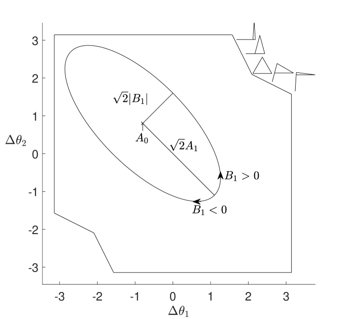
Figure 7: A schematic diagram of an elliptical path in the space of non-self-intersecting configurations ($\Delta\theta_{1}$, $\Delta\theta_{2}$) for a three-link body, symmetric about the line $\Delta\theta_{1}=-\Delta\theta_{2}$. $A_{0}$ is the average of $\Delta\theta_{1}$ over the ellipse and $\sqrt{2}A_{1}$ and $\sqrt{2}|B_{1}|$ are the semi-major and semi-minor axes of the ellipse. The sign of $B_{1}$ gives the direction in which the path is traversed.

Within this space of paths, we consider a low-dimensional subspace—motions that have a single frequency (i.e. time-harmonic motions)—and are symmetric about the line $\Delta\theta_{1}=-\Delta\theta_{2}$. This symmetry guarantees no net rotation over a period (see appendix A), so the long-time trajectory of the body is a straight line rather than a circle. Such paths are described by

$$\Delta\theta_{1}(t)=A_{0}+A_{1}\cos(2\pi t)+B_{1}\sin(2\pi t),\quad\Delta\theta_{2}(t)=-A_{0}-A_{1}\cos(2\pi t)+B_{1}\sin(2\pi t),\quad 0\leq t\leq 1.$$ (27)

The three parameters $A_{0},A_{1}$, and $B_{1}$ describe an ellipse with center $(A_{0},-A_{0})$ and principal semiaxes $A_{0}$ and $|B_{0}|$ (figure 7). We assume $A_{0}\geq 0$ without loss of generality, so the motion starts at the lower right region instead of the upper left region of the ellipse (but the same path is traversed in either case). The sign of $B_{1}$ gives the direction (clockwise or counterclockwise) around the path. Changing the sign of $B_{1}$ reverses time and thus reverses the motion (when $\mu_{b}=\mu_{f}$, as here), giving the same efficiency.

We compute motions over the region of $(A_{0},A_{1},B_{1})$-space giving admissible paths (ellipses that lie in the region of figure 7). To solve a large number of motions quickly, it is efficient to first compute a velocity map (or “connection” KaMaRoMe2005a ; HaCh2010a ; JiAl2013 )—a map from the shape variables ($\Delta\theta_{1}$, $\Delta\theta_{2}$) and their velocities ($\dot{\Delta\theta}_{1}$, $\dot{\Delta\theta}_{2}$) to the body velocities at the tail $\{\dot{x}_{0}(t),\dot{y}_{0}(t),\dot{\theta}_{0}(t)\}$, from which we can reconstruct the body motion via (13)-(14) at each time and thus the efficiency. Because of the scaling relation (19), instead of computing $\{\dot{x}_{0}(t),\dot{y}_{0}(t),\dot{\theta}_{0}(t)\}$ over the four-dimensional space ($\Delta\theta_{1}$, $\Delta\theta_{2}$, $\dot{\Delta\theta}_{1}$, $\dot{\Delta\theta}_{2}$) it is enough to compute the tail velocities over two three-dimensional spaces ($\Delta\theta_{1}$, $\Delta\theta_{2}$, $\dot{\Delta\theta}_{1}$) with $|\dot{\Delta\theta}_{1}|\leq 1$ and $\dot{\Delta\theta}_{2}=1$; and ($\Delta\theta_{1}$, $\Delta\theta_{2}$, $\dot{\Delta\theta}_{2}$) with $\dot{\Delta\theta}_{1}=1$ and $|\dot{\Delta\theta}_{2}|\leq 1$, and then obtain the tail velocities at other combinations of ($\dot{\Delta\theta}_{1}$, $\dot{\Delta\theta}_{2}$) by rescaling them into one of these three-dimensional spaces (if $\mu_{b}\neq\mu_{f}$ two additional maps would be needed, at $\dot{\Delta\theta}_{1}=-1$ and $\dot{\Delta\theta}_{2}=-1$).

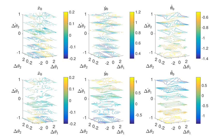
Figure 8: Contour plots showing the three components of the velocity map ($\dot{x}_{0}$, $\dot{y}_{0}$, and $\dot{\theta}_{0}$) as functions of body shape and motion parameters (top row) $\Delta\theta_{1}$, $\Delta\theta_{2}$, and $\dot{\Delta\theta_{2}}$ when $\dot{\Delta\theta_{1}}$ = 1 or (bottom row) $\Delta\theta_{1}$, $\Delta\theta_{2}$, and $\dot{\Delta\theta_{1}}$ when $\dot{\Delta\theta_{2}}$ = 1.

In figure 8 we show the two sets of velocity maps used to construct $\{\dot{x}_{0}(t),\dot{y}_{0}(t),\dot{\theta}_{0}(t)\}$ for any values of body shape variables and their velocities when $\dot{\Delta\theta}_{1}=1$ (top row) and $\dot{\Delta\theta}_{2}=1$ (bottom row). The contours in each slice plane show that the quantities vary relatively smoothly in these spaces, despite the sharp variations in frictional forces. We have observed from more extensive data that they are apparently continuous with bounded derivatives, but that their derivatives change sharply where the regularization parameter is important, i.e. where static friction plays a role.

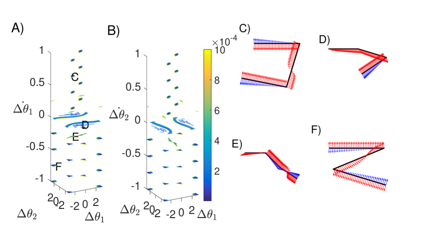
Figure 9: Regions in the space of body shape and motion parameters where static friction regularization model is involved. A) and B) Contours show regions where the body speed lies between 0 and $10^{-3}$ over at least one of the three links, in the space of (A) $\Delta\theta_{1}$, $\Delta\theta_{2}$, and $\dot{\Delta\theta}_{2}$ when $\dot{\Delta\theta}_{1}$ = 1 or (B) $\Delta\theta_{1}$, $\Delta\theta_{2}$, and $\dot{\Delta\theta}_{1}$ when $\dot{\Delta\theta}_{2}$ = 1. C, D, E, and F) Representative examples of body shapes and motions (labeled in A) where static friction regularization model is involved. Distributions of body velocities (blue) and frictional forces (red) are shown.

Static friction is potentially important when the speed ($\|\partial_{t}\mathbf{X}\|$) is of the order of the regularization parameter ($\delta=10^{-4}$) over one or more entire links. If instead small velocities do not occur, or occur only at discrete points on the body, $\delta$ has only a small effect on the net forces and torque. In figure 9 we show regions in the velocity map spaces where static friction is important. Although the regions are small, they are involved in the motions that optimize efficiency, described in the next section. The regions can be classified into a small number of cases. Typical examples are shown in panels C–F, with corresponding labels in panel A. Case C occurs when $\Delta\theta_{1}$ and $\Delta\theta_{2}$ are approximately equal to $\pi/2$ or $-\pi/2$. The forces from the outer links are nearly equal and opposite, but a small net force and torque is needed from the middle link to balance those on the outer links. Case D represents a broad region where one of the link angle velocities ($\dot{\Delta\theta}_{1}$ or $\dot{\Delta\theta}_{2}$) is zero and the other link angle is bent sharply (with magnitude between $\pi/2$ and $\pi$) and has nonzero velocity. Case E represents a smaller region where one of the link angles has a small but nonzero velocity. Case F occurs when the link angles have magnitudes near $\pi$ and opposite signs. To understand why static friction is involved we look at cases C and F more closely.

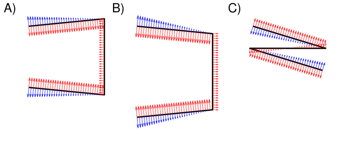
Figure 10: Examples of symmetric body motions where the static friction regularization model is involved. Distributions of body velocities (blue) and frictional forces (red) are shown.

Figure 10A and B show symmetric examples similar to figures 9C and 4. The outer links provide forces that are nearly opposite and in the vertical direction, but have a small horizontal component. Due to the top-bottom symmetry of the configuration, the velocity of the middle link can only be horizontal for the vertical forces to balance. Without regularization, the horizontal force per unit length on the middle link could only be 0 or $\pm 1$, which cannot balance the small horizontal forces from the outer links. Regularization allows for a smaller horizontal force with a nearly static middle link, like the force from static friction. Figure 10C shows a symmetric version of figure 9F—symmetric with respect to reflection through the body center. The outer links provide forces that are equal and opposite, but give a small net torque. To provide a torque with zero net force, the middle link has a purely rotational motion. Without regularization the force density on the middle link could only be 0, or -1 on one half and 1 on the other, giving a net torque of 0 or $\pm 1/36$ (since the link has length 1/3). Regularization allows a different torque to be obtained with a nearly static middle link, like that due to static friction. The other cases in figure 9 are more difficult to explain because they are not symmetric.

We now compute the distance traveled, work done, and their ratio $\lambda$, the efficiency, for the elliptical trajectories shown in figure 7, parametrized by $A_{0},A_{1},$ and $B_{1}$. To aid our presentation we begin by showing in figure 11 the results in the two-parameter space with $A_{0}=0$. These are for motions that are symmetric with respect to the line $\Delta\theta_{1}=\Delta\theta_{2}$, but there is no reason a priori to prefer such motions.

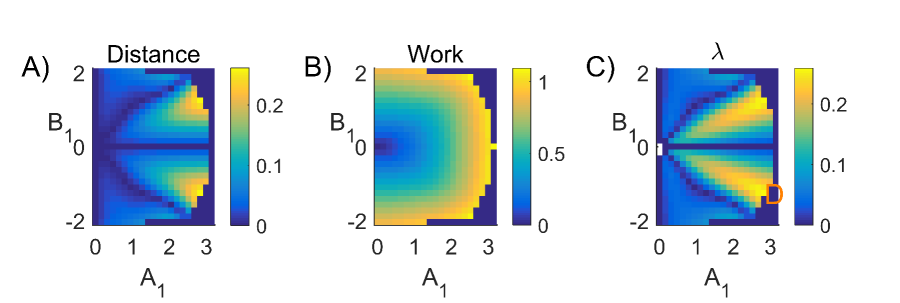
Figure 11: Plots of (A) the distance traveled, (B) the work done against friction, and (C) the efficiency $\lambda$ (distance/work) for elliptical paths with $A_{0}=0$.

Figure 11A shows that the distance traveled per period is largest for a localized region of motions at the limit of self-contact. The dark blue region beyond the outer boundary of the shaded region gives coefficients for motions that involve self-contact. The distance is nearly zero for motions near the line $A_{1}=B_{1}$, i.e. circular trajectories. These trajectories approximate the traveling-wave motions shown in the previous section, and are effective for low Reynolds number swimming Pu1977a ; BeKoSt2003a ; TaHo2007a ; AvRa2008a given the 2:1 drag anisotropy of slender swimming bodies lauga2009hydrodynamics . The line $A_{1}=0$ corresponds to standing wave motions similar to that in the previous section, and results in zero distance traveled since the motion is the same but the trajectory is reversed under time reversal. The line $B_{1}=0$ gives standing wave motions that are antisymmetric about the body midpoint but also unchanged under time reversal, and thus also give zero net distance traveled.

Panel B shows the work done per period, which has a much simpler distribution—it is nearly radially symmetric. Larger coefficients $A_{1}$ and $B_{1}$ are clearly correlated with larger sweeping motions of the links. The work done has no obvious relationship with the distance traveled (A), because the net translation (0.261 body lengths at maximum) is only a small contribution to the total motion in most cases. The efficiency (C) has a pattern similar to the distance, though of course smaller-amplitude motions are weighted more favorably. Nonetheless, the most efficient motion is close to the distance-maximizing motion, and has efficiency 0.259. The quantities are invariant when the sign of $B_{1}$ is changed, because the motion is simply reversed in time.

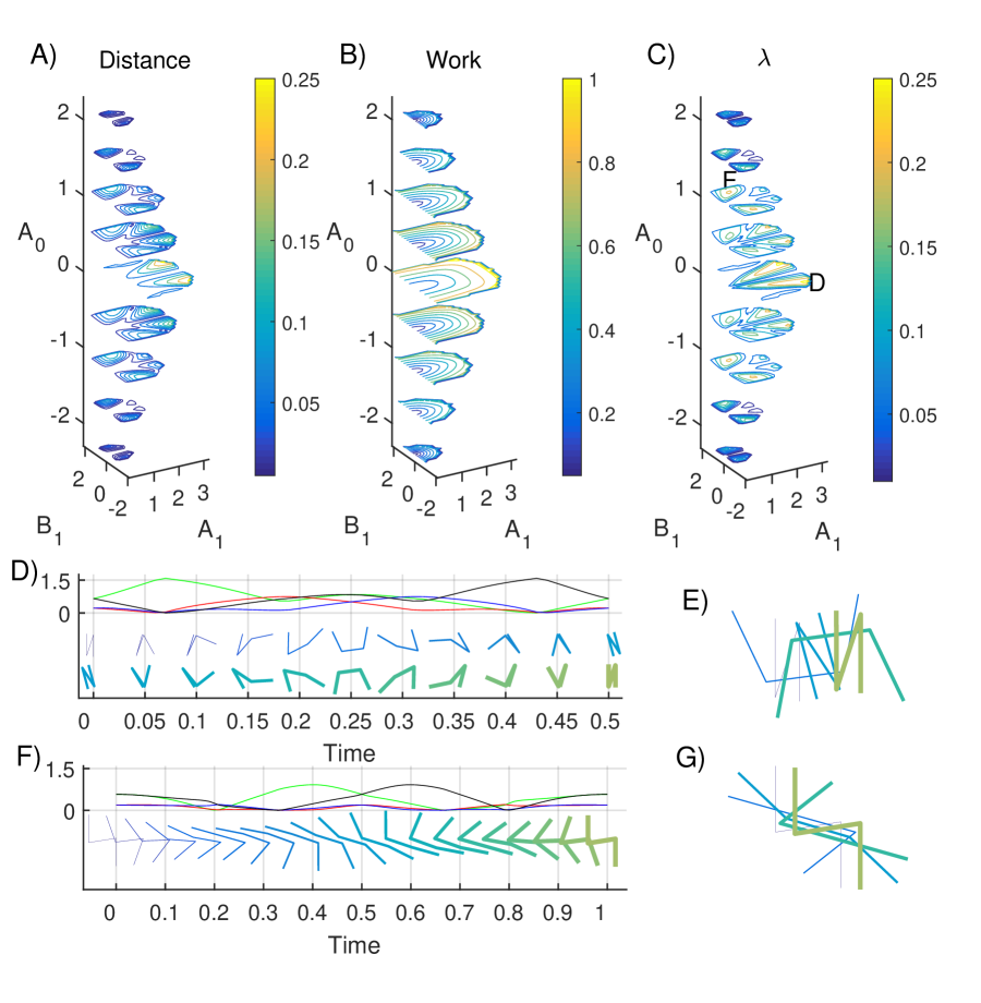
Figure 12: Contour plots of (A) the distance traveled, (B) the work done against friction, and (C) the efficiency $\lambda$ (distance/work) for elliptical paths with various $A_{0}$. D) For the most efficient symmetric elliptical body motion (labeled ‘D’ in panel C and Fig. 11C), the top four lines show the speeds of the four link endpoints (from tail to head: black, blue, red, and green). Below are snapshots of the body during the first (top row) and second (bottom row) half-periods. E) A subset of snapshots from panel D in the lab frame. F) For the motion giving the second best local optimum in efficiency (labeled ‘F’ in panel C), the same data as in panel D. G) A subset of snapshots from panel F in the lab frame.

In figure 12A-C we show the same quantities but with $A_{0}$ varied over its full range. At the middle of the $A_{0}$ axis is $A_{0}=0$, so there the contour plots show the same data as in the previous figure. When $A_{0}=0$, the largest distance is achieved at a point with $A_{1}>B_{1}$. As $A_{0}$ increases or decreases (moving up or down the vertical axis), another local maximum, this one having $B_{1}>A_{1}$ gives a larger distance. In panel B, the work maintains an approximate radial symmetry, and does not depend strongly on $A_{0}$ (which varies the offset bias but not the sweeping amplitude of the links’ motions). In panel C, the efficiency has three local maxima. The global maximum is found at $A_{0}$ = 0, has efficiency 0.259, and is labeled ‘D’ (here and in the previous figure). The motion is shown in panels D and E. The second best local optimum is found at $A_{0}$ = 1.1, has efficiency 0.207, and is labeled ‘F’. The motion is shown in panels F and G. The third local optimum (not shown) has $A_{0}$ = 2.5, efficiency 0.094. In panel D, the snapshots of the globally optimal motion are arranged in two rows: first half-period (top) and second half-period (bottom), for which the body shape is a mirror image of that in first half-period ($\Theta$ has opposite sign). The snapshots are shown at equal time intervals during the half-periods (time is labeled at the bottom). At the top are four colored lines showing the speeds of the four endpoints of the three links versus time for the first half-period. We see that at two times, 0.07 and 0.43, three of the four endpoints (and two of the three links) are almost static. Here the static friction regularization is involved in the force balance. At $t$ = 0.07, one link extends rightward while the other two remain fixed. At $t$ = 0.43, one link is retracted rightward towards the other two. The snapshots are shown at their true locations in the lab frame in panel E; the body moves about 0.26 body lengths. For the second local optimum, the snapshots are shown in panel F, in time increments of 0.05 over an entire period. Near $t$ = 0.33 and 0.67, two of the links are almost static, while the third link moves in the direction of locomotion. The motion is shown in the lab frame in panel G. The distance traveled is about 37% of that in panel E and the work done is about 47%. Both of the optimal motions can be described as follows: One of the outer links is rotated forward (i.e. in the direction of locomotion), with the other two mostly static (for $t$ = 0.38-0.5 in D, 0.2-0.5 in F), then the other outer link is rotated forward with the other two mostly static (from $t$ = 0-0.12 in D, 0.5-0.8 in F), then the middle link is moved, which requires the two outer links to rotate (from $t$ = 0.12-0.38 in D, 0.8-1 and 0-0.2 in F). The motions are roughly speaking similar to concertina motion, where the snake moves part of its body (like one of the outer links) forward, pushing off of (or pulling towards) the rest of the body (like the other two links) that is held fixed by static friction, forming an “anchor” gray1946mechanism ; jayne1986kinematics ; jayne1991kinematics . Because the body has only three links, moving the middle link forward requires all three links to move and rotate, so this part of the motion is somewhat distinct.

VI Optimal motions

Inspired by the concertina-like motions in the previous section, we now look for more general smooth motions that can achieve the highest possible efficiency for any inextensible body, not necessarily one with three links. First, we show that an upper bound on efficiency for any motion is the reciprocal of the smallest friction coefficient (1 in the isotropic case).

The distance traveled by the body (16) is the same for all $s$ since the body moves as a translation without rotation after one period. Thus we can write

$$d=\left\|\int_{0}^{1}\int_{0}^{1}\partial_{t}\mathbf{X}(s,t)dsdt\right\|.$$ (28)

The work done against friction is (17) with $\mathbf{f}$ from (7). Let $u_{s}\equiv\partial_{t}\mathbf{X}\cdot\hat{\mathbf{s}}$ and $u_{n}\equiv\partial_{t}\mathbf{X}\cdot\hat{\mathbf{n}}$. We have

$$-\mathbf{f}(s,t)\cdot\partial_{t}\mathbf{X}(s,t)=\frac{\mu_{t}u_{n}^{2}+\mu_{s}u_{s}^{2}}{\sqrt{u_{s}^{2}+u_{n}^{2}}}$$ (29)

where

$$\mu_{s}(s,t)\equiv\left(\mu_{f}H(\widehat{\partial_{t}{\mathbf{X}}}\cdot\hat{\mathbf{s}})+\mu_{b}(1-H(\widehat{\partial_{t}{\mathbf{X}}}\cdot\hat{\mathbf{s}}))\right).$$ (30)

Therefore

$$-\mathbf{f}(s,t)\cdot\partial_{t}\mathbf{X}(s,t)\geq\min(\mu_{t},\mu_{f},\mu_{b})\sqrt{u_{s}^{2}+u_{n}^{2}}=\min(\mu_{t},\mu_{f},\mu_{b})\|\partial_{t}\mathbf{X}(s,t)\|$$ (31)

and

$$W\geq\min(\mu_{t},\mu_{f},\mu_{b})\int_{0}^{1}\int_{0}^{1}\|\partial_{t}\mathbf{X}(s,t)\|dsdt\geq d\,\min(\mu_{t},\mu_{f},\mu_{b}).$$ (32)

so

$$\lambda=\frac{d}{W}\leq\frac{1}{\min(\mu_{t},\mu_{f},\mu_{b})}.$$ (33)

This upper bound corresponds to a body that translates uniformly in the direction of lowest friction. Such a motion cannot have zero net force for nonzero friction, but we now show simple motions that satisfy the equations of motion and saturate this upper bound in the limit of a small parameter, for any choice of friction coefficients, including the isotropic case. These are concertina-like motions, in the sense that part of the body forms an anchor, remaining static due to static friction, allowing the rest of the body to be pushed or pulled forward.

Figure 13: Motions and performance of optimally efficient crawlers. A) Snapshots of the crawler during the first half-period of motion. The circle and square are the endpoints of the bump region, and the triangle is the body midpoint. B) Snapshots during the second half period. C) Plot of work done against friction over one period outside the bump region (“Work_outer”, red), that done inside the bump region (“Work_inner”, blue), the total work (black), and the distance covered in one period (green), versus the bump region width parameter $\epsilon$. D) The efficiency $\lambda=$ Work/Distance versus the bump region length $\epsilon$. E) Snapshots of an efficient (symmetric) crawler when $\mu_{t}$ is the smallest friction coefficient.

We first assume isotropic friction. The body is initially straight (see figure 13A, top). The motion has three stages. In stage one, a straight segment in the rear half of the body but near the midpoint (between the circle and triangle in figure 13A) forms a “bump.” It deforms from straight to curved, but keeping the tangent angles at its endpoints unchanged, so the endpoints get closer. This pulls the rear of the body forward, because the front portion (front half) of the body (the “anchor”) is static due to static friction. If the front portion of the body slides with an $O(1)$ velocity, the rear portion of the body is not large enough to provide a balancing force. Therefore, the front portion of the body’s velocity is O($\delta$). At the end of stage one (red body in panel A), the bump reaches its maximum amplitude. In stage two (from the red body to the blue body), the bump travels forward along the body, to the region between the triangle and the square. The blue shape is thus a mirror image of the red shape. Here the body endpoints do not move, because the region away from the bump (left of the circle and right of the square) is an anchor. Stage three (from the blue body to the last straight configuration in A) is essentially the reverse of stage one—the bump flattens out, pushing the region in front of the square forward, with the back region of the body fixed because now it is an anchor. The net result is that the body has moved rightward some amount (which can be seen comparing the body endpoints over the sequence of motions). In addition to moving rightward, the body undergoes a much smaller vertical displacement and rotation because the bump is upward. To achieve a motion with zero net rotation (and zero net vertical displacement), we then perform the mirror image of the motion (panel B) for $0.5\leq t\leq 1$, with $\Theta(s,t+0.5)=-\Theta(s,t)$. Then we see that the mirror image motion in the lab frame is a solution:

$$\dot{\theta}_{0}(t+0.5) =-\dot{\theta}_{0}(t),\partial_{t}\theta(s,t+0.5)=-\partial_{t}\theta(s,t),$$ (34)

$$\dot{y}_{0}(t+0.5) =-\dot{y}_{0}(t),\partial_{t}y(s,t+0.5)=-\partial_{t}y(s,t),$$ (35)

$$\dot{x}_{0}(t+0.5) =\dot{x}_{0}(t),\partial_{t}x(s,t+0.5)=\partial_{t}x(s,t).$$ (36)

We have the same horizontal displacement but the vertical displacement and rotation are reversed. Panel B shows the snapshots in the simulation of the second half of the motion (at the beginning/end of the three stages only). The length of the bump (half the arc-length distance from the circle to the square) is a control parameter $\epsilon$ that we can shrink to zero. We show now that the distance traveled is proportional to $\epsilon$, and the work done can be decomposed into two parts. The work done inside the bump region (left of the circle and right of the square) is proportional to $\epsilon^{2}$ (blue squares in panel C). The velocities in the bump region $\sim\epsilon$, the frictional force density $\sim 1$, and the bump region length $\sim\epsilon$, so by (17)

$$W_{\mbox{inner}}\sim\int_{0}^{1}\int_{0.5-\epsilon}^{0.5+\epsilon}1\cdot\epsilon dsdt=O(\epsilon^{2}).$$ (37)

The work done outside the bump region ($W_{\mbox{outer}}$, red crosses in C) approaches the distance traveled (green triangles) as $\epsilon\to 0$, and both are proportional to $\epsilon$. $W_{\mbox{outer}}$ is approximately the unit frictional force density times the body speed in the region outside the bump multiplied by the length of that region $\sim 1$:

$$W_{\mbox{outer}}\sim\int_{0}^{1}\int_{\{0\leq s\leq 0.5-\epsilon\}\cup\{0.5+\epsilon\leq s\leq 1\}}1\cdot\partial_{t}x(s,t)dsdt\sim d.$$ (38)

Adding (37) and (38) we have $\lambda=1+O(\epsilon)$. This is shown in panel D for the motions in panels A-B. When $\epsilon$ decreases below 0.1, we find it is necessary to decrease the numerical regularization parameter $\delta$ from $10^{-4}$ to $10^{-6}$ or $10^{-8}$ so it does not affect the results (i.e. so $\delta$ is much smaller than the typical speed of body deformation).

Now assume the friction coefficients are anisotropic. If the smallest friction coefficient is either $\mu_{f}$ or $\mu_{b}$, then the body should be oriented in panels A-B so that the lower of $\mu_{f}$ and $\mu_{b}$ applies for motion to the right. If instead the smallest friction coefficient is $\mu_{t}$, then we bend the body so that it has two bump regions, and the outer regions are oriented transverse to the direction of locomotion (see figure 13E). By symmetry, motion is solely in the horizontal direction (the mirror image stroke in panel B is not required now). Snapshots are shown only at the beginning/end of each stage in panel E. With anisotropic friction, the above estimate for $W_{\mbox{inner}}$ (37) is multiplied by $\max(\mu_{t},\mu_{f},\mu_{b})$ to obtain an upper bound, while that for $W_{\mbox{outer}}$ (38) is multiplied by $\min(\mu_{t},\mu_{f},\mu_{b})$. The global upper bound for $\lambda$ (33) is achieved in the limit $\epsilon\to 0$.

We have assumed an inextensible body. For an extensible body, a one-dimensional version of the above motion is obtained by projecting the body density distribution at each instant onto the horizontal axis. Similar longitudinal motions are used by certain soft-bodied animals (e.g. worms) that alternately contract and extend longitudinal muscles keller1983crawling . Snakes, however, are nearly inextensible due to their backbone lillywhite2014snakes .

VII Conclusion

In this work we have studied the locomotion of bending and sliding bodies under isotropic friction. We developed a regularization approach to handle cases where static friction is needed to find a solution. We also introduced a fixed-point iteration method that can compute the body tail velocities robustly from all initial guesses without the need for a line search method. We first used the method to show that the most efficient motions with anisotropic friction—traveling wave deformations—lead to little or no locomotion with isotropic friction. Next, we used the method to compute the velocity map for the three-dimensional body shape and shape velocity spaces of a three-link crawler. We used these maps to obtain a general picture of the locomotion efficiency landscape for the 3D space of coefficients giving symmetrical elliptical paths in the space of the body link angles. We found that static friction regularization is involved in small (but important) regions of the velocity map and described their necessity in symmetric cases. The distance traveled and efficiency are very small for motions corresponding to standing waves or traveling waves. The efficiency has three local maxima, and the top two (0.21 and 0.26) occur at motions that are similar to concertina locomotion—a sequence of motions in which one of the links moves forward while the other two links remain almost motionless.

We then proposed a class of concertina-like motions that saturate the upper bound for efficiency for any choice of friction coefficients. The optimal smooth motions of section VI require short wavelengths $\sim\epsilon$ (and large frequencies $\sim 1/\epsilon$ to travel an $O(1)$ distance), which explains why the numerical optimization using 45 or 190 modes in AlbenSnake2013 did not converge to such motions. It is interesting, however, that in the optimal time-harmonic motions with only three links, concertina-like motions can be seen. Although static friction arises in the optimal motions shown here, we believe that solutions with similar motions—and similar efficiencies—may exist with only the kinetic friction model (i.e. without regularization). In other words, the motion may be altered so that instead of remaining static, the “anchor” portion of the body slides slowly but has enough kinetic friction to balance that on the remainder of the body.

Appendix A Zero net rotation for motions symmetric with respect to $\Delta\theta_{1}=-\Delta\theta_{2}$.

We show here that motions of three-link bodies that are symmetric with respect to the line $\Delta\theta_{1}=-\Delta\theta_{2}$ (e.g. figure 7) result in zero net rotation over a period. For such motions we can assume (as in section V) that the body motion starts on the line $\Delta\theta_{1}=-\Delta\theta_{2}$ in configuration space (by shifting time by a constant if necessary), so the body lies on this line at $t$ = 0 and 1, and at $t$ = 1/2 by the symmetry of the path. The symmetry implies that the link angle differences at $t$ and $1-t$ are related by $\Delta\theta_{1}(t)=-\Delta\theta_{2}(1-t)$ and $\Delta\theta_{2}(t)=-\Delta\theta_{1}(1-t)$. Thus if the three links at time $t$ have tangent angles $\{\theta_{0}(t),\theta_{0}(t)+\Delta\theta_{1}(t),\theta_{0}(t)+\Delta\theta_{1}(t)+\Delta\theta_{2}(t)\}$ then those at $1-t$ have tangent angles $\{\theta_{0}(1-t),\theta_{0}(1-t)-\Delta\theta_{2}(t),\theta_{0}(1-t)-\Delta\theta_{2}(t)-\Delta\theta_{1}(t)\}$. This implies that $\theta(s,t)-\theta(1-s,1-t)=\theta_{0}(t)+\Delta\theta_{1}(t)+\Delta\theta_{2}(t)-\theta_{0}(1-t)$, which is independent of $s$. In other words, the body at time $1-t$ has the same shape (tangent angle) as that at time $t$, up to an overall rotation, when the body at time $1-t$ is viewed from the opposite end—starting at $s=1$ and ending at $s=0$. If we define a new coordinate $u=1-s$, we can describe the tangent angle at time $1-t$ in a body frame running from $u=0$ to $u=1$ using the function $\Theta_{u}(u,t)$ as

$$\theta(u,1-t)=\theta_{u=0}(1-t)+\Theta_{u}(u,1-t).$$ (39)

We have $\Theta(s,t)=\Theta_{u}(1-s,1-t)$ and $\partial_{t}\Theta(s,t)=-\partial_{t}\Theta_{u}(1-s,1-t)$, so in the body frames the two shapes are the same and their rates of change are opposite. Therefore, following the solution procedure described below equations (13)-(14), the solutions for the rotation rates at $s=0$ and $u=0$ are opposite (if $\mu_{b}=\mu_{f}$):

$$\dot{\theta}_{s=0,b}(t)=-\dot{\theta}_{u=0,b}(1-t)$$ (40)

Here $b$ denotes body frame, but these are also the rotation rates in the lab frame as discussed below equations (13)-(14):

$$\dot{\theta}_{s=0}(t)=\dot{\theta}_{s=0,b}(t)=-\dot{\theta}_{u=0,b}(1-t)=-\dot{\theta}_{u=0}(1-t).$$ (41)

We can use these results to compute the net rotation from $t=0$ to $t=1$ (over a period), $\theta_{s=0}(1)-\theta_{s=0}(0)$. Since the body has $\Delta\theta_{1}=-\Delta\theta_{2}$ at $t$ = 0, 1/2, and 1, at those times the tangent angle at $u=0$ (in the direction of increasing $u$) is that at $s=0$ plus $\pi$:

$$\theta_{s=0}(1)-\theta_{s=0}(0) =\theta_{u=0}(1)+\pi-\theta_{u=0}(1/2)+\theta_{u=0}(1/2)-\theta_{s=0}(0)$$ (42)

$$=\theta_{u=0}(1)-\theta_{u=0}(1/2)+\theta_{s=0}(1/2)-\theta_{s=0}(0)$$ (43)

$$=\int_{1/2}^{1}\dot{\theta}_{u=0}(t)dt+\int_{0}^{1/2}\dot{\theta}_{s=0}(t)dt$$ (44)

$$=\int_{1/2}^{1}-\dot{\theta}_{s=0}(1-t)dt+\int_{0}^{1/2}\dot{\theta}_{s=0}(t)dt$$ (45)

$$=\int_{1/2}^{0}\dot{\theta}_{s=0}(w)dw+\int_{0}^{1/2}\dot{\theta}_{s=0}(t)dt$$ (46)

$$=0,$$ (47)

where $w=1-t$. In words, whatever rotation occurs from $t=0$ to 1/2 is undone from 1/2 to 1, when we view the body from the opposite end.

References

- [1] J Gray. The mechanism of locomotion in snakes. Journal of Experimental Biology, 23(2):101–120, 1946.
- [2] J Gray and HW Lissmann. The kinetics of locomotion of the grass-snake. Journal of Experimental Biology, 26(4):354–367, 1950.
- [3] Bruce C Jayne. Kinematics of terrestrial snake locomotion. Copeia, pages 915–927, 1986.
- [4] John J Socha. Kinematics: Gliding flight in the paradise tree snake. Nature, 418(6898):603–604, 2002.
- [5] R L Hatton and H Choset. Generating gaits for snake robots: annealed chain fitting and keyframe wave extraction. Autonomous Robots, 28(3):271–281, 2010.
- [6] Hamidreza Marvi and David L Hu. Friction enhancement in concertina locomotion of snakes. Journal of The Royal Society Interface, 9(76):3067–3080, 2012.
- [7] Michael H Dickinson, Claire T Farley, Robert J Full, MAR Koehl, Rodger Kram, and Steven Lehman. How animals move: an integrative view. Science, 288(5463):100–106, 2000.
- [8] Christel Hohenegger and Michael J Shelley. Stability of active suspensions. Physical Review E, 81(4):046311, 2010.
- [9] Sarah D Olson, Susan S Suarez, and Lisa J Fauci. Coupling biochemistry and hydrodynamics captures hyperactivated sperm motility in a simple flagellar model. Journal of theoretical biology, 283(1):203–216, 2011.
- [10] Sookkyung Lim and Charles S Peskin. Fluid-mechanical interaction of flexible bacterial flagella by the immersed boundary method. Physical Review E, 85(3):036307, 2012.
- [11] Shannon K Jones, Young JJ Yun, Tyson L Hedrick, Boyce E Griffith, and Laura A Miller. Bristles reduce the force required to ‘fling’wings apart in the smallest insects. Journal of Experimental Biology, 219(23):3759–3772, 2016.
- [12] Yoseph Bar-Cohen. Biomimetics: biologically inspired technologies. CRC Press, 2005.
- [13] Bojan Jakimovski. Biologically inspired approaches for locomotion, anomaly detection and reconfiguration for walking robots, volume 14. Springer, 2011.
- [14] DT Roper, S Sharma, R Sutton, and P Culverhouse. A review of developments towards biologically inspired propulsion systems for autonomous underwater vehicles. Proceedings of the Institution of Mechanical Engineers, Part M: Journal of Engineering for the Maritime Environment, 225(2):77–96, 2011.
- [15] Francois Jacob. Evolution and tinkering. Science, 196(4295):1161–1166, 1977.
- [16] R McNeill Alexander. Optima for animals. Princeton University Press, 1996.
- [17] R Brian Langerhans and David N Reznick. Ecology and evolution of swimming performance in fishes: predicting evolution with biomechanics. Fish locomotion: an eco-ethological perspective, pages 200–248, 2010.
- [18] L E Becker, S A Koehler, and H A Stone. On self-propulsion of micro-machines at low Reynolds number: Purcell’s three-link swimmer. Journal of Fluid Mechanics, 490(1):15–35, 2003.
- [19] J E Avron, O Gat, and O Kenneth. Optimal swimming at low Reynolds numbers. Physical Review Letters, 93(18):186001, 2004.
- [20] D Tam and A E Hosoi. Optimal stroke patterns for Purcell’s three-link swimmer. Physical Review Letters, 98(6):68105, 2007.
- [21] Henry C Fu, Thomas R Powers, and Charles W Wolgemuth. Theory of swimming filaments in viscoelastic media. Physical Review Letters, 99(25):258101, 2007.
- [22] Saverio E Spagnolie and Eric Lauga. The optimal elastic flagellum. Physics of Fluids, 22:031901, 2010.
- [23] Darren Crowdy, Sungyon Lee, Ophir Samson, Eric Lauga, and AE Hosoi. A two-dimensional model of low-Reynolds number swimming beneath a free surface. Journal of Fluid Mechanics, 681:24–47, 2011.
- [24] Brian Bittner, Ross L Hatton, and Shai Revzen. Geometrically optimal gaits: a data-driven approach. Nonlinear Dynamics, 94(3):1933–1948, 2018.
- [25] James Lighthill. Mathematical Biofluiddynamics. SIAM, 1975.
- [26] Stephen Childress. Mechanics of swimming and flying. Cambridge University Press, 1981.
- [27] JA Sparenberg. Hydrodynamic Propulsion and Its Optimization:(Analytic Theory), volume 27. Kluwer Academic Pub, 1994.
- [28] S. Alben. Passive and active bodies in vortex-street wakes. Journal of Fluid Mechanics, 642:95–125, 2009.
- [29] Sébastien Michelin and Stefan G Llewellyn Smith. Resonance and propulsion performance of a heaving flexible wing. Physics of Fluids, 21:071902, 2009.
- [30] J. Peng and S. Alben. Effects of shape and stroke parameters on the propulsion performance of an axisymmetric swimmer. Bioinspiration and Biomimetics, 7:016012, 2012.
- [31] Mattia Gazzola, Médéric Argentina, and Lakshminarayanan Mahadevan. Gait and speed selection in slender inertial swimmers. Proceedings of the National Academy of Sciences, 112(13):3874–3879, 2015.
- [32] Z V Guo and L Mahadevan. Limbless undulatory propulsion on land. Proceedings of the National Academy of Sciences, 105(9):3179, 2008.
- [33] Jeffrey Aguilar, Tingnan Zhang, Feifei Qian, Mark Kingsbury, Benjamin McInroe, Nicole Mazouchova, Chen Li, Ryan Maladen, Chaohui Gong, Matt Travers, Ross L Hatton, Howie Choset, Paul B Umbanhowar, and Daniel I Goldman. A review on locomotion robophysics: the study of movement at the intersection of robotics, soft matter and dynamical systems. Reports on Progress in Physics, 79(11), 2016.
- [34] Harvey B Lillywhite. How Snakes Work: Structure, Function and Behavior of the World’s Snakes. Oxford University Press, 2014.
- [35] Bruce C Jayne. Mechanical behaviour of snake skin. Journal of Zoology, 214(1):125–140, 1988.
- [36] Richard A Seigel, Joseph T Collins, and Susan S Novak. Snakes: ecology and evolutionary biology. Macmillan New York etc., 1987.
- [37] D L Hu, J Nirody, T Scott, and M J Shelley. The mechanics of slithering locomotion. Proceedings of the National Academy of Sciences, 106(25):10081, 2009.
- [38] D L Hu and M Shelley. Slithering Locomotion. In Natural Locomotion in Fluids and on Surfaces, pages 117–135. Springer, 2012.
- [39] Daniel I Goldman and David L Hu. Wiggling through the world: The mechanics of slithering locomotion depend on the surroundings. American Scientist, 98(4):314–323, 2010.
- [40] Aksel Andreas Transeth, Remco I Leine, Christoph Glocker, Kristin Ytterstad Pettersen, and Pål Liljebäck. Snake robot obstacle-aided locomotion: Modeling, simulations, and experiments. IEEE Transactions on Robotics, 24(1):88–104, 2008.
- [41] Aksel Andreas Transeth, Kristin Ytterstad Pettersen, and Pål Liljebäck. A survey on snake robot modeling and locomotion. Robotica, 27(07):999–1015, 2009.
- [42] Hidetaka Ohno and Shigeo Hirose. Design of slim slime robot and its gait of locomotion. In Intelligent Robots and Systems, 2001. Proceedings. 2001 IEEE/RSJ International Conference on, volume 2, pages 707–715. IEEE, 2001.
- [43] Pål Liljebäck, Kristin Ytterstad Pettersen, Øyvind Stavdahl, and Jan Tommy Gravdahl. A review on modelling, implementation, and control of snake robots. Robotics and Autonomous Systems, 60(1):29–40, 2012.
- [44] Felix L Chernousko. Modelling of snake-like locomotion. Applied mathematics and computation, 164(2):415–434, 2005.
- [45] Gregory L Wagner and Eric Lauga. Crawling scallop: Friction-based locomotion with one degree of freedom. Journal of theoretical biology, 324:42–51, 2013.
- [46] Eric Lauga and Thomas R Powers. The hydrodynamics of swimming microorganisms. Reports on Progress in Physics, 72(9):096601, 2009.
- [47] S Alben. Optimizing snake locomotion in the plane. Proc. Roy. Soc. A, 469(2159):1–28, 2013.
- [48] Geoffrey Ingram Taylor. Analysis of the swimming of long and narrow animals. Proc. R. Soc. Lond. A, 214(1117):158–183, 1952.
- [49] Michael Sfakiotakis and Dimitris P Tsakiris. Undulatory and pedundulatory robotic locomotion via direct and retrograde body waves. In Robotics and Automation, 2009. ICRA’09. IEEE International Conference on, pages 3457–3463. IEEE, 2009.
- [50] Ryan D Maladen, Yang Ding, Paul B Umbanhowar, and Daniel I Goldman. Undulatory swimming in sand: experimental and simulation studies of a robotic sandfish. The International Journal of Robotics Research, 30(7):793–805, 2011.
- [51] F Jing and S Alben. Optimization of two- and three-link snake-like locomotion. Physical Review E, 87(2):022711, 2013.
- [52] RG Cox. The motion of long slender bodies in a viscous fluid. Part 1. General theory. Journal of Fluid Mechanics, 44(04):791–810, 1970.
- [53] Xiaolin Wang, Matthew T Osborne, and Silas Alben. Optimizing snake locomotion on an inclined plane. Physical Review E, 89(1):012717, 2014.
- [54] Xiaolin Wang and Silas Alben. Dynamics and locomotion of flexible foils in a frictional environment. Proc. R. Soc. A, 474(2209):20170503, 2018.
- [55] Bharat Bhushan. Introduction to tribology. John Wiley & Sons, 2013.
- [56] Valentin L Popov. Contact mechanics and friction. Springer, 2010.
- [57] Ettore Pennestrì, Valerio Rossi, Pietro Salvini, and Pier Paolo Valentini. Review and comparison of dry friction force models. Nonlinear dynamics, 83(4):1785–1801, 2016.
- [58] CT Kelley. Iterative methods for linear and nonlinear equations. Society for Industrial and Applied Mathematics, 1995.
- [59] JE Dennis Jr and Robert B Schnabel. Numerical Methods for Unconstrained Optimization and Nonlinear Equations, volume 16. SIAM, 1996.
- [60] James K Hopkins, Brent W Spranklin, and Satyandra K Gupta. A survey of snake-inspired robot designs. Bioinspiration & Biomimetics, 4(2):021001, 2009.
- [61] E M Purcell. Life at low Reynolds number. Am. J. Phys, 45(1):3–11, 1977.
- [62] J E Avron and O Raz. A geometric theory of swimming: Purcell’s swimmer and its symmetrized cousin. New Journal of Physics, 10:063016, 2008.
- [63] E Kanso, J E Marsden, C W Rowley, and J B Melli-Huber. Locomotion of articulated bodies in a perfect fluid. Journal of Nonlinear Science, 15(4):255–289, 2005.
- [64] R L Hatton and H Choset. Connection vector fields and optimized coordinates for swimming systems at low and high Reynolds numbers. In Proceedings of the ASME Dynamic Systems and Controls Conference (DSCC), Cambridge, Massachusetts, USA, 2010.
- [65] Bruce C Jayne and James D Davis. Kinematics and performance capacity for the concertina locomotion of a snake (coluber constrictor). Journal of Experimental Biology, 156(1):539–556, 1991.
- [66] Joseph B Keller and Meira S Falkovitz. Crawling of worms. Journal of Theoretical Biology, 104(3):417–442, 1983.