SimFS: A Simulation Data Virtualizing
File System Interface

Abstract

Nowadays simulations can produce petabytes of data to be stored in parallel filesystems or large-scale databases. This data is accessed over the course of decades often by thousands of analysts and scientists. However, storing these volumes of data for long periods of time is not cost effective and, in some cases, practically impossible. We propose to transparently virtualize the simulation data, relaxing the storage requirements by not storing the full output and re-simulating the missing data on demand. We develop SimFS, a file system interface that exposes a virtualized view of the simulation output to the analysis applications and manages the re-simulations. SimFS monitors the access patterns of the analysis applications in order to (1) decide the data to keep stored for faster accesses and (2) to employ prefetching strategies to reduce the access time of missing data. Virtualizing simulation data allows us to trade storage for computation: this paradigm becomes similar to traditional on-disk analysis (all data is stored) or in situ (no data is stored) according with the storage resources that are assigned to SimFS. Overall, by exploiting the growing computing power and relaxing the storage capacity requirements, SimFS offers a viable path towards exa-scale simulations.

I Motivation

Reliable long-term data archiving is very costly. For example, storing 10 TiB for 10 years costs between $2,400 and $6,000 on Microsoft’s Azure. The only practical scheme to mitigate these costs, besides deletion, is (lossy or lossless) compression of the data and it is fundamentally constrained by the tradeoff between data size and quality. When taking a closer look at how data is generated, we observe two fundamentally different modes: (1) data collected by sensors or terminals that observe non-deterministic environments or (2) data generated by deterministic simulations that model complex and potentially chaotic systems. We observe, that the latter could be recomputed on demand instead of stored, given the right data retrieval system.

Many simulation applications produce vast amounts of data that is today stored in large filesystems or databases. For example, the European Centre for Medium-Range Weather Forecasts (ECMWF) alone had an archive of 100 PiB in 2015, experiencing an annual growth rate of 45% [1]; by 2020, their archive will reach a Zettabyte. Climate model data is used by countries and insurances to make critical decisions thus repeatability of analyses is mandated by international regulatory bodies. Astrophysics simulations are another example where data volumes grow with the compute capabilities, creating more than 20 PiB of data each [2]. Thousands of such simulations are collected in virtual observatories, mainly limited by the storage costs [3, 4]. Those two examples outline a clear trend: As we proceed into the age of simulation [5], big (simulation) data will soon be required for many real-world decisions.

The data produced by large simulations is commonly used by thousands of analysts and scientists over the course of decades. They are used in analysis workflows where the data is stored in files or databases. Specifically, these workflows address two requirements: (1) data can conveniently be analyzed with any access pattern (e.g., time-reverse or random access) and (2) the exact same data can (often years) later be re-analyzed to reproduce the results. This makes the data-backed analysis a de-facto standard for today’s simulation data analytics.

We propose SimFS, a file system interface that virtualizes simulation output data for analysis tools. SimFS avoids storing the whole simulation output data but stores checkpoints to re-start parts of the simulation and produce missing files on demand. A virtualized view, similar to virtual memory, is provided to the analysis tools, enabling them to work as if all output data exists as files. This way, SimFS can exploit the tradeoff between inflexible in-situ analysis, where all analyses are running together with the simulation and no data is stored, and on-disk, where the full simulation output is stored and no re-simulations are needed. Figure 1 shows the expected costs for performing 100 analyses equally spaced over varying data availability periods for a real-world climate simulation scenario discussed in detail in Sec. V-A. It shows that SimFS can reduce the costs for a five-year period from more than $200,000 for an on-disk solution to less than $100,000. We also show “in-situ”, which re-runs the whole simulation for each analysis as comparison.

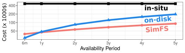
Figure 1: Aggregated analysis cost. The cost of the different analysis solutions (on-disk, in-situ, SimFS) is function of the time period over which the analyses are executed.

Implementing SimFS poses interesting challenges that we describe in the following. In the past, computation speeds and cost efficiency grew much faster than storage speeds and efficiency. Whether this trend continues or not, SimFS must always adjust to the exact cost and performance tradeoff. While the file-system virtualization itself is simple, SimFS employs complex caching and prefetching strategies to adjust the tradeoff between computation (resimulation) and storage cost. To guide optimizations, it exposes a set of interfaces that can be used in addition to the fully transparent virtualization to optimize client applications as, e.g., guided prefetching or non-blocking reads. By nature of the virtualization, SimFS transparently enables large-scale analyses on multi-petabyte datasets on terabyte storage systems that have been impossible so far. Thus, SimFS not only enables new scientific breakthroughs but it also allows the system cost to shrink with the computation costs.

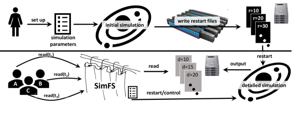
Figure 2: Overview of SimFS

Figure 2 shows the abstract workflow of SimFS: The simulation is initially set up by a scientist (top left of Figure 2) and runs to completion while producing restart files (black files, top right). First in-situ analyses may be performed during the initial simulation but we focus on later analyses. Later, analysis tools from different clients (e.g., researchers in the lower left) access the virtualization layer through standard data-access interfaces such as HDF5 [6], netCDF [7], or ADIOS [8]. SimFS manages the simulations to re-create output data (gray files, bottom) on demand and delivers it to the analysis tools. We remark that simulations can be restarted on different devices than the original simulation, e.g., smaller GPU systems, because the simulated time intervals are less demanding.

SimFS requires that the simulation can be re-started from checkpoints and delivers a bitwise-identical output to the original run. While checkpoint/restart facilities are already needed to deal with limited compute time and failures, bitwise reproducibility may not generally be available. However, it should generally be used for good scientific practice (repeatability) and can be achieved with a set of standard techniques without significant performance penalty [9, 10]. If bitwise reproducibility cannot be guaranteed, we expect the analyses being able to operate on data that is different from the one produced by the initial simulation. The analysis can check if the re-simulated data differs by using the SimFS APIs.

We argue that SimFS solves a significant part of the big data storage challenge in simulation sciences. We will show how it even improves analysis performance and automatically utilizes available storage resources efficiently, all without requiring any modifications of the analysis tools. SimFS is used on some of the largest machines existing today.

II Virtualizing Simulations

Virtualizing simulation data is very similar to virtual memory and paging, a key component in today’s operating systems: the simulation output is our virtual memory and the pages are sets of simulation output files. If an application accesses a file that is not on disk (i.e., swapped out), then the entire page containing that file has to be re-simulated. (i.e., loaded). While memory is virtualized by means of memory loads and stores, we virtualize simulation data by intercepting calls to I/O libraries. In this model, SimFS acts like a memory management unit but on a coarser grain.

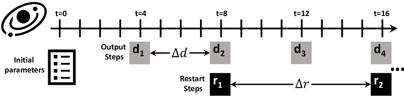
Figure 3: Simulate time, output, and restart steps.

II-A Modeling Simulations

Our model focuses on forward-in-time simulations. They generate one or more output steps during the run, each of which contains one or more timesteps. A single time step can encapsulate multiple smaller simulation steps that are not visible in the output steps, hence not exposed in our model. Furthermore, simulators commonly provide the ability to write restart steps that can be used to restart a simulation. Output and restart steps are stored in files.

As simulations proceed in timesteps $t_{1}$, $t_{2}$, $\ldots$, $t_{n}$, a simulator configuration is defined by $\Delta d$, that is the number of timesteps between two output steps, and $\Delta r$, that is the number of timesteps between two restart steps. Each output step contains all $\Delta d-1$ timesteps beginning from either the last output step or the beginning of the simulation. We assume that the simulation can be restarted from any restart step and proceeds forward in time. Thus, to produce an output step $d_{i}$, the simulation needs to be started from the closest previous restart step $R(d_{i})=\lfloor\frac{i\cdot\Delta d}{\Delta r}\rfloor$. To exploit spatial locality, we let a re-simulation run until at least the next restart step $\lceil\frac{i\cdot\Delta d}{\Delta r}\rceil$. Choosing $\Delta d$ and $\Delta r$ allows us to adjust the time-space tradeoff. If SimFS stores all output steps, we can serve all requests from the output files directly. However, we assume that we cannot store the complete output on disk. Then, $\Delta d$ selects the granularity of the data generation and $\Delta r$ the time to reach a specific timestep. In particular, the bigger the $\Delta r$, the lower the number of restart files that need to be stored and the higher the average time to simulate a specific output step.

Figure 3 shows an example where a simulation starts from $t=0$ and runs forward-in-time beyond $t=16$ (not shown in the figure). Each output step contains four timesteps ($\Delta d=4$) and can be restarted every 8 timesteps ($\Delta r=8$).

Simulation Contexts Simulation output characteristics (i.e., output steps content, $\Delta d$, $\Delta r$) are determined by a specific simulation configuration and a simulator can have multiple configurations. We define a simulation context as a simulator and an its configuration. Since the analysis applications operate on the simulation output produced by a given context, simulation contexts are a central component of our model.

Multiple simulation contexts can share the same restart files, offering different simulation outputs that can be produced at different speeds. Analyses can be interested in one or more simulation output types, hence in one or more simulation contexts: e.g., analyzing a coarser grain simulation output on a simulation context and then switch to finer grain on a different context for a more detailed study of interesting events.

For a given simulation, scientists identify multiple simulation contexts that are made available to the analyses through SimFS. Since each simulation context can produce different subset of output steps, they can lead to different re-simulations costs. The analyses can specify their simulation context via an environment variables or the SimFS APIs.

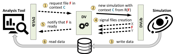
Figure 4: Handling misses in SimFS. Dashed arrows are control messages (TCP/IP); solid (thin) arrows represent actions (script execution); solid (bold) arrows represent data movement (file system).

III SimFS

SimFS consists of two components: (1) the Data Virtualizer (DV), a daemon process that coordinates simulations and analyses and (2) the DV Library (DVLib), that enables the analyses and simulations to communicate and synchronize with the DV. DVLib provides bindings for many I/O libraries (e.g., netCDF, HDF-5) so the analyses and simulations can be transparently interfaced to the DV. Moreover, it exposes a set of APIs to let virtualization-aware analysis applications have a more direct control on the virtualized environment.

III-A Virtualized Simulation Output Analysis

Analysis accesses to the simulation output are intercepted by DVLib, which communicates with the DV to check if the requested files are available. After intercepting an open call issued by an analysis application, the DVLib sends a request to the DV and waits for a response. If the file exists, then an acknowledgment is sent back to the application, which is now free to open the file. Figure 4 shows the case in which the requested file is not available. Once DV receives the request and checks that the file is not available, it starts a new re-simulation, configured according with the context specified by the analysis application. The new simulation starts producing output steps, writing them on the (parallel) file system. DVLib is aware of the files created by the running simulation since it intercepts the close calls issued by it. Once a file is closed, DVLib assumes that this file is ready on disk and notifies the DV of this event. When notified, DV checks if there are analysis applications waiting for the file and, if yes, it forwards the notification to them. After receiving the notification from DV, the DVLib running on the analysis call unblocks and perform the original I/O library call that will now find the file on disk.

A key motivation of virtualizing simulations output is to enable the analysis of datasets that are one or more orders of magnitude larger than the available storage capacity. This implies that SimFS has to monitor the data volume occupied by a simulation context and eventually evict output steps when the given storage resources are saturated. In particular, we associate each simulation context with a storage area (i.e., a file system directory). When a new re-simulation from a given context is launched, DVLib intercepts the create calls from the simulator and redirects them to the associated storage area. The simulation context also specifies the maximum size of its storage area. When the actual size of a storage area reaches its maximum size, the DV applies eviction policies (see Sec. III-D) for selecting one or more output steps to evict. SimFS associates a reference counter to each output step to keep track of the analysis that are currently accessing it. An output step can be evicted only if its reference counter is zero.

III-B Simulator Interface

The DV is in charge to restart simulations to produce data that is being accessed by the analysis applications but not on disk. However, how to configure and start a simulation is strictly related to the simulator and to the system where the simulation has to be run (e.g., how to set start and stop output steps; how to submit the simulation job to the batch system). To let a simulator be managed by SimFS we introduce a simulation driver that can be implemented as a LUA script and provides the following simulator-specific functionalities:

• Naming Convention: The output steps file names follow a convention that is specified by the simulator and its configuration. SimFS needs to be able to compare filenames for, e.g., finding the closest in time restart step from which the simulation can be restarted to produce a missing file. The simulation driver provides a function $key$ that given a filename, returns a integer key such that if the output step $d_{i}$ is produced after $d_{j}$ by the simulator, then $key(d_{i})>key(d_{j})$.

• Simulation Job: When creating a new simulation, SimFS invokes a simulation driver function that takes as arguments the simulation start and stop output steps keys and the parallelism level. This function creates a script that the DV can execute to start the new simulation. SimFS needs to tune the simulation parallelism to enable the optimizations described in Sec. IV-B. However, the simulator can impose constraints on its resources allocation (e.g., square or power of two number of processes). By using the parallelism level parameter, that is an integer from $0$ to max parallelism level (i.e., a parameter set by the simulation driver), SimFS can increase the simulation parallelism without having to directly enforce these constraints, which are instead enforced by the simulator-specific implementation of the simulation interface.

We intercept the create and close calls issued by the simulator to let the DV trigger replacement policies and analysis notifications, respectively. The mapping of these calls to standard I/O libraries is reported in Table I.

III-C Analysis Application Interface

The analysis applications are interfaced to the DV through DVLib. DVLib provides bindings to standard I/O libraries, allowing legacy analysis applications to transparently access virtualized simulation output, and a set of APIs that can be used by virtualization-aware analysis applications.

III-C1 Transparent Mode

DVLib provides mappings to standard I/O libraries to enable analysis of virtualized simulation output without requiring code changes to the analysis applications or simulators. This is achieved by intercepting the open, create, read, and close calls of the different I/O libraries. Table I shows the function names of these calls for the different I/O libraries we provide bindings for. When DVLib intercepts an open call, it sends a request to the DV that checks whether the file exists. If not, a new simulation is restarted as in Sec. III-A. This call is non-blocking, even if the opened file is not on disk. When the applications tries to read from a file that is not on disk, DVLib blocks the call (by not returning from it) until the DV sends a notification of the file being ready. The close call is intercepted to let DV decrease the output step. The simulation context name accessed by an analysis transparently interfaced to SimFS can be specified as an environment variable.

Call	(P)NetCDF [7]	(P)HDF5 [6]	ADIOS [8]
open	nc(mpi)_open	H5Fopen	adios_open (r)
create	nc(mpi)_create	H5Fcreate	adios_open (w)
read	nc(mpi)_vara_get_type	H5Dread	adios_schedule_read
close	nc(mpi)_close	H5Fclose	adios_close

TABLE I: Mapping data access operations to I/O libraries

III-C2 SimFS APIs

SimFS provides an additional API providing more information and control about the virtualized environment. These functions do not perform I/O: they are issued before the I/O calls to coordinate with the DV before accessing the files.

Initialize/Finalize: An analysis tool can start an analysis on a given simulation context by calling the SIMFS_Init function. Multiple contexts can be open by the same application.

⬇

int SIMFS_Init(char * sim_context, SIMFS_Context * context);

int SIMFS_Finalize(SIMFS_Context * context);

Requesting Data: Before accessing a set of files with standard I/O libraries, the analysis acquires such files with the SIMFS_Acquire function. This function blocks until the DV notifies that the requested files are available. A non-blocking version of the call is available that does not wait for the requests files to become available: the application must then explicitly test or wait for data availability.

⬇

int SIMFS_Acquire(SIMFS_Context context, char * filenames[],

int count, SIMFS_Status * status);

int SIMFS_Acquire_nb(SIMFS_Context context,

char * filenames[], int count, SIMFS_Status * status,

SIMFS_Req * req);

int SIMFS_Release(SIMFS_Context context, char * filename);

The acquire functions return a SIMFS_Status object containing information such as the error state (e.g., restart failed) and the estimated waiting time for the requested files to become available. The analysis can use this information for debugging, profiling, and for saving compute hours/energy (e.g., by checkpointing itself and requesting to be resumed after the estimated waiting time). Once the analysis of a file finishes, the application releases it with a SIMFS_Release call.

Waiting for Data: The application can wait or test for the completion of non-blocking acquire calls with the SIMFS_Wait and SIMFS_Test functions, respectively. These functions return a SIMFS_Status object to inform the application about the status of the re-simulation. Since an acquire request can target multiple files with different states (i.e., on disk or missing), we provide the SIMFS_Waitsome and SIMFS_Testsome calls that allow to receive availability information for a subset of files requested in the acquire call.

⬇

int SIMFS_Wait(SIMFS_Req * req, SIMFS_Status * status);

int SIMFS_Test(SIMFS_Req * req, int * flag,

SIMFS_Status * status);

int SIMFS_Waitsome(SIMFS_Req * req, int * readycount,

int readyidx[], SIMFS_Status * status);

int SIMFS_Testsome(SIMFS_Req * req, int * readycount,

int readyidx[], SIMFS_Status * status);

Comparing Data: If bitwise reproducibility is not guaranteed, the analysis can check if a given file matches the one produced by the initial simulation with the SIMFS_Bitrep call. The check is made by comparing the checksums of the current file and the original one. The way the checksum is computed is simulator-specific and specified as a function of simulator driver. The simulation context keeps a map from filenames to checksums that can be updated through a command line utility at the time when the first simulation is run.

⬇

int SIMFS_Bitrep(SIMFS_Context context, char * filename,

int * flag);

III-D Caching Simulation Data

Simulation data virtualization is sufficient to fully solve data storage limitations because it allows to freely adjust the space-time-tradeoff by re-creating data on demand. Yet, re-simulating every file may be too slow and with limited disk-space, it is unclear which files should remain on disk and which should be re-created on demand.

Traditional caching theory classifies cache misses using the 3Cs model [11] as compulsory, capacity, and conflict misses. In our model, we first run a whole simulation to create restart files and these initial compulsory misses cannot be avoided. Conflict misses are caused by low-latency caching schemes that map blocks to sets to optimize the performance. Since our system is operating on a milliseconds time-frame, we employ fully associativity, avoiding conflict misses. However, if the data does not fit in cache, we may need to evict files from the cache due to the limited storage, causing capacity misses.

Caching simulation data is different from caching memory accesses in system caches: here, a cache miss leads to the re-simulation of a number of output steps which depends on the restart interval and the missing output step. Also, the replacement schemes need to take into account that may not be possible to evict some output steps if they are currently referenced by one or more analyses. We now discuss a set of known replacement schemes that we extend to fulfill the requirements for simulation data virtualization.

Locality-Based (LRU/LIRS/ARC): Least-Recently-Used (LRU) is one of the most common and simplest replacement schemes. The idea is to keep track of the recency of each cache entry (i.e., how many accesses have been issued from the last access to it) and select the least recently used one as victim. More advanced locality-based schemes have been proposed with the aim of improving over LRU. The key change is in how locality is defined (LRU defines it as recency). Low Inter-reference Recency Set (LIRS) [12] leverages both recency and reuse distance (i.e., number of accesses between two consecutive accesses targeting the same entry) for selecting entries to replace. Instead, Adaptive Replacement Cache (ARC) [13] distinguishes entries that are frequently used from the ones that have been recently accessed: they are kept in two different sets which size is adjusted at runtime in order to adapt to the observed access pattern.

Cost-Aware (BCL/DCL): The Basic Cost-Sensitive LRU (BCL) and Dynamic Cost-Sensitive LRU (DCL) replacement schemes have been proposed by Jeong et al. [14]. The main idea is that they do not evict the LRU if there is a more recent entry with a lower miss cost: the victim is selected as the first entry in the recency-ordered list with a cost lower than the one of the LRU. LRU is used as fallback if no evictable entry can be find in this search. If the LRU is not evicted, its cost gets reduced to avoid the case in which a costly, sporadically-accessed entry leads to the eviction of too many cheaper, highly-reused entries. In this context, the miss cost of an entry (i.e., output step) is the distance, in number of output steps, from its closest previous restart step. BCL and DCL differ by the time at which the LRU depreciation takes place: BCL depreciates it as soon as the LRU is not evicted, while DCL does that only if an evicted non-LRU entry gets accessed before the LRU. Jeong et al. propose also the Adaptive Cost-Sensitive LRU (ACL) but we choose to not consider this algorithm since it is not designed for fully associative caches.

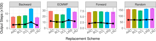
Figure 5: Cache replacement schemes comparison for different access patterns.

Caching Schemes Evaluation: To evaluate the discussed caching schemes we virtualize a 4-days simulation producing an output step every $5$ minutes and a restart file every $4$ hours. The SimFS’s cache is set to $25\%$ of the data volume.

The simulation data is accessed by a synthetic analysis tool that replicates a given access trace. We generate different traces for different analysis patterns: forward, where a set of output steps are accessed on a forward-in-time trajectory; backward, where the output steps are accessed on backward-in-time trajectory; random, where the accessed output steps are randomly selected. For each access pattern, we generate $50$ traces starting their analysis at a random point of the simulation timeline and accessing a different numbers of output steps (randomly selected between $100$ and $400$). We then concatenate all the single traces in a single one to be replicated by our synthetic analysis tool. In addition, we extract traces from the ECMWF archive [1] that provides a complete trace of all successful accesses to the ECFS archival system from January 2012 to May 2014. The resulting trace accesses $874$ different files for a total of $659,989$ times.

Figure 5 shows the re-simulation statistics: the bars represent the number of simulated output steps for the different replacement schemes (x-axis) and different access patterns (tiles). We also report the number of times a new simulation has been restarted to satisfy the analysis (black points). We repeat each experiment $100$ times, generating new traces each time, and report the median and the 95% CI of the measured counts. Except for LIRS, we notice no important differences among the caching schemes for scan-like access patterns (i.e., forward and backward). LIRS performs worse in the backward case because it prioritizes the eviction of files that are most likely to be accessed with this trajectory. The cost-based schemes, in particular DCL, minimize the number or restarts/produced output steps in the ECMWF and random cases. Since multiple analysis tools accessing data with different access patterns can be interfaced to SimFS at the same time, we expect that the random and ECMWF traces to be the most similar to real-word scenarios. Hence, in the following, we fix the caching replacement scheme to DCL.

III-E Virtualizing Simulation Pipelines

Many scientific simulation are organized in stages: e.g., the initial boundary conditions are copied from long-term storage to start a coarse-grain simulation that outputs data that is then used as input of a finer-grain simulation. If we virtualize the fine-grain simulation output we may need to re-simulate parts of it, needing the output of the coarser-grain one. However, storing all the output of the coarse-grain simulation to re-simulate any portion of the fine-grain one may be prohibitive, leading us to our initial problem (i.e., we cannot keep all the data on-disk).

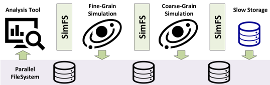
Figure 6: Using SimFS to virtualize simulation pipelines

We have two options to address this problem: 1) the simulation job of the fine-grain simulation makes sure that all the needed input is on disk (e.g., by starting the coarser-grain simulation first or by copying it from long-term storage); 2) we virtualize the output of all the stages, as shown in Figure 6. In the second case we define a simulation context for each stage: if the fine-grain simulation accesses a part of its input that is missing, then a coarse-grain re-simulation will be started. Similarly, if the coarser-grain simulation accesses missing parts of its input, then a new simulation job will be created: in this case, this job will not start a simulation but just issue the copy of the data from the long-term storage area.

IV Optimizing Simulation Data Accesses

Many analysis tools access the data with simple traversal schemes such as forward or backward in time trajectories. These access patterns can be optimized using prefetching strategies that can hide the simulation startup latency as well as improve the overall production bandwidth. These prefetching strategies can be used to adjust another resource-performance tradeoff. For example, in the common case where the simulation produces data slower than the analysis tool can consume it, we can use more resources to run many simulations in parallel and match the analysis application ingestion bandwidth.

IV-A Performance Model

We start by defining a performance model for the simulations and the analysis applications that is then used in the proposed optimizations. The idea is to have a general performance model that allows us to not make particular assumptions on the simulator and analysis.

Restarting a simulation may incur in non-functional delays such as waiting for resources (e.g., VM deploying or queuing time in a batch system), reading the restart file, and initializing the simulation model. We define $\alpha_{\text{sim}}(p)$ as the restart latency of a simulation running with parallelism level $p$. Once started, the simulation writes the output step on disk with a certain frequency: we model the simulation inter-production time as $\tau_{\text{sim}}(p)$, that represents the time between the production of two consecutive output steps. In the following, we omit $p$ for both $\alpha_{\text{sim}}(p)$ and $\tau_{\text{sim}}(p)$ if not required by the context. According to this model, the time needed to simulate $n$ output steps using a parallelism level $p$ is: $T_{\mathrm{sim}}(n,p)=\alpha_{\mathrm{sim}}(p)+n\cdot\tau_{\mathrm{sim}}(p)$. Hence, the time to produce an output step $d_{i}$ is the simulation time from $R(d_{i})$ to $d_{i}$ itself: $T_{\mathrm{sim}}(i-R(d_{i}),p)$.

We model the analysis application performance as $\tau_{\text{cli}}^{k}$, that is the time between two consecutive k-strided accesses.

IV-B Prefetching Simulation Data

We associate each analysis application that is interfaced to SimFS with a prefetch agent. The prefetch agent monitors the application access pattern, measures $\tau_{\text{cli}}^{k}$, and can prefetch new re-simulations. Forward and backward access patterns are detected after two $k$-stride consecutive accesses. Once a pattern is detected, the agent starts prefetching re-simulations according with the monitored parameters. A prefetch agent resets itself whenever the analysis tool changes its analysis direction and/or stride, or terminates.

IV-B1 Prefetching forward-in-time accesses

We start with the simplest and most common pattern: forward-in-time. This pattern is directly supported by in-situ, where the analysis tool runs in tandem with the simulation. While a single simulation with in-situ analysis is always faster than re-simulation, SimFS has many benefits if the data needs to be analyzed at varying times (e.g., by different analysis). In fact, we can improve this scenario at two fronts: (1) we can use all the storage available to cache output steps for future analyses and (2) we can reduce the analysis completion time using prefetching.

Masking Restart Latency

A forward-in-time analysis reads the files in the same time trajectory they are produced by the simulation. If no prefetching strategies are adopted, SimFS starts a new simulation only when a miss occurs, making the analysis application wait the full restart latency at every miss.

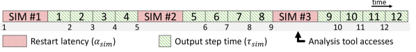
Figure 7: Forward analysis without prefetching.

Figure 7 shows an example of an analysis making a sequence of ($k=1$)-strided accesses with all of them resulting in a miss. The simulation has a restart interval of $\Delta r=4$ timesteps, the restart latency is $\alpha_{\text{sim}}=2$ time units, and produces one output step every time unit ($\tau_{\text{sim}}=1$ time unit). The analysis consumes the output steps twice as fast as they are produced ($\tau_{\text{cli}}^{k}=1/2$ time units). The accessed output steps are reported into the gray bar at the bottom. The example shows how the accesses performed by the analysis are delayed of the the restart latency every time a miss occurs. We want to mask the restart latency by overlapping it with the analysis, as shown in Figure 8. This leads to two questions: How long does the re-simulation need to be? and When to trigger a new re-simulation?

The re-simulation length $n$ is the number of output steps that one re-simulation produces. The number of $k$-stride accesses that can be served by one re-simulation is $\lfloor\frac{n}{k}\rfloor$. The analysis processing time per output step is $\max(k\cdot\tau_{\text{sim}},\tau_{\text{cli}}^{k})$: it can be limited by either the simulation’s or its own speed. We want to find an $n$ such that the time spent in analyzing $\lfloor\frac{n}{k}\rfloor$ output steps covers the restart latency of the next re-simulation, reserving the first two accesses to confirm the prefetching validity (i.e., same direction and stride). This $n$ can be found by satisfying the following inequality:

$$\left(\Bigl{\lfloor}\frac{n}{k}\Bigr{\rfloor}-2\right)\cdot\max(k\cdot\tau_{\text{sim}},\tau_{\text{cli}}^{k})\geq\alpha_{\text{sim}}$$

Hence, $n$ needs to be: $n\geq\Bigl{\lceil}\frac{\alpha_{\text{sim}}}{\max(k\cdot\tau_{\text{sim}},\tau_{\text{cli}}^{k})}+2\Bigr{\rceil}\cdot k$. We always round $n$ up to the nearest restart interval multiple:

$$n=R\left(\Bigl{\lceil}\frac{\alpha_{\text{sim}}}{\max(k\cdot\tau_{\text{sim}},\tau_{\text{cli}}^{k})}+2\Bigr{\rceil}\cdot k+\frac{\Delta r}{\Delta d}\right)$$

The abstraction we want to provide to the analysis tool is as if there is a single simulation serving all the non-cached output steps it requests. Hence, we need to prefetch a new re-simulation just in time to mask its restart latency. Since the prefetch agents see the time as discretized by the (strided) analysis accesses, we prefetch at the time of the last $k$-strided access that allows the masking of the restart latency. This output step, named prefetching step, is computed as: $d_{i}+n-\Bigl{\lceil}\frac{\alpha_{\text{sim}}}{\max(k\cdot\tau_{\text{sim}},\tau_{\text{cli}}^{k})}\Bigr{\rceil}\cdot k$, where $d_{i}$ is the initial output step of the currently running simulation.

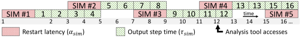
Figure 8: Hiding simulation restart latency.

Matching Analysis Bandwidth

While the hiding of the restart latency avoids delaying the analysis at every miss, the analysis can still be faster in consuming the output steps than the simulation in producing them: $\tau_{\text{sim}}>\frac{\tau_{\text{cli}}^{k}}{k}$. In this case, we can improve the simulation production bandwidth by using two strategies: (1) Increase the simulation parallelism level, or (2) start multiple simulations in parallel.

Strategy (1) is the first strategy that a prefetch agent employs if the analysis is faster than the simulation. When the application is accessing the output steps produced by a simulation (i.e., due to a miss), the prefetch agent monitors both $\tau_{\text{cli}}^{k}$ and $\tau_{\text{sim}}(p)$: whenever the analysis is faster than the simulator, the prefetch agent increases $p$ for the next re-simulation that will be started to recover the misses of this analysis. Whenever the prefetch agents determines that there are no performance benefits in increasing $p$ or the max parallelism level is reached, it switches to strategy (2).

Strategy (2) runs multiple re-simulations in parallel to increase the simulation output bandwidth. The ideal number of parallel re-simulations needed to match the analysis bandwidth is: $s_{\text{opt}}=\lceil{k\cdot\tau_{\text{sim}}}/{\tau_{\text{cli}}^{k}}\rceil$. Figure 9 shows how this strategy changes the example of Sec. IV-B1: the prefetch agent now starts $s_{\text{opt}}=2$ new re-simulations at each prefetching step and, after the first batch of prefetched simulations (i.e., accessed output step $9$), the analysis can run at its full bandwidth. However, this strategy can lead SimFS to launch a large number of re-simulations if the analysis is much faster than the simulation. Also, it is not guaranteed that the prefetched output steps will be accessed by the analysis, which can terminate or change its direction/stride at any time. To limit this issue, a simulation context can be configured to not prefetch directly $s_{\text{opt}}$ simulations at time, but start with $s=1$ and double it at each prefetching step until the analysis stays on the same direction/stride and $s<\min(s_{\text{opt}},s_{\text{max}})$, where $s_{\text{max}}$ is a simulation context parameter that limits the maximum number of simulations that can be running at the same time.

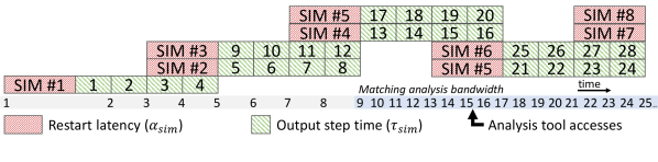
Figure 9: Hiding restart latency and matching forward analysis bandwidth.

IV-B2 Prefetching backward-in-time accesses

Backward-in-time accesses are common in root-cause analysis. They are conceptually similar to forward-in-time but require a different prefetching scheme because the simulation itself is always forward-in-time. Because of this, the analysis cannot operate in tandem with the simulation (like in-situ): if $d_{i}$ is missing, the analysis has to wait until the re-simulation produces the output steps from $R(d_{i})$ to $d_{i}$, like in forward-in-time trajectories. However, since the analysis goes backward, now it can find other output steps produced in that interval already in cache. The output steps produced after $d_{i}$ (i.e., from $d_{i+1}$ to $R(d_{i}+\Delta r)$) are not useful to the analysis. Hence, prefetching for backward-in-time analysis requires to mask not only the restart latency but also (part of) the re-simulation itself.

Let us consider the case where the analysis is slower than the simulation: $\frac{\tau_{\mathrm{cli}}^{k}}{k}>\tau_{\mathrm{sim}}$. To hide the re-simulation time, we have to simulate enough output steps such that the time the analysis needs to consume them is higher than the cost of the next simulation: $\frac{n}{k}\cdot\tau_{\mathrm{cli}}^{k}\geq\alpha_{\mathrm{sim}}+n\cdot\tau_{\mathrm{sim}}$. Hence, the minimum number of output steps to be simulated is: $n=\frac{k\cdot\alpha_{\mathrm{sim}}}{\tau_{\mathrm{cli}}^{k}-k\cdot\tau_{\mathrm{sim}}}$, rounded up to the next restart step.

If the analysis is faster than the simulation, then we have again two strategies: increase the simulation parallelism or run multiple simulations in parallel. The ideal number of parallel re-simulation we need to match a backward-in-time analysis bandwidth is different from the forward-in-time case. Here, once a missing output step is produced, the analysis can find in cache all the next output steps on its trajectory up to the restart step used for the last re-simulation. Hence, we want to produce a number of output steps such that the time the analysis takes to process them (at its full speed) is greater than the time to prefetch a new set of output steps:

$$s\cdot\frac{n}{k}\cdot\tau_{\mathrm{cli}}^{k}\geq\alpha_{\mathrm{sim}}+n\cdot\tau_{\mathrm{sim}}$$

hence, the minimum number of parallel simulations is:

$$s=\frac{k\cdot\alpha_{\mathrm{sim}}}{n\cdot\tau_{\mathrm{cli}}^{k}}+\frac{k\cdot\tau_{\mathrm{sim}}}{\tau_{\mathrm{cli}}^{k}}$$

This introduces a trade-off between $s$ and $n$: the higher the multiple parallel simulations ($s$). the lower the number of output steps per simulation ($n$) that are needed to match the backward-in-time analysis bandwidth. However, reducing $n$ by using more computing resources in parallel allows us to reduce the time needed to reach the full bandwidth. Figure 10 shows a backward analysis with $\alpha_{\text{sim}}=2$, $\tau_{\text{sim}}=1$, $\tau_{\text{cli}}^{k}=1/2$, $k=1$, and $n=4$. In this case, the minimum number of parallel resimulation needed to match the analysis bandwidth is $s=3$. The example shows how a new batch of re-simulations (SIM #5,6,7) can be overlapped to the analysis of the output steps produced by the previous one (SIM #2,3,4).

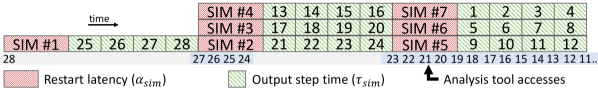
Figure 10: Hiding restart latency and matching backward analysis bandwidth.

IV-C Prefetching Effectiveness

The discussed prefetching strategies aim to hide the restart overhead and increase the overall simulation bandwidth. However, to avoid a too aggressive prefetching that would lead to cache pollution, SimFS tries to kill simulations prefetched by analyses that terminated or changed analysis direction (e.g., from forward to backward or jumped to a different timespan). A simulation can be killed only if there are no other analyses waiting for the files that are going to be produced by it. Additionally, SimFS tries to detect cache pollution by monitoring the accesses to the prefetched output steps: if an analysis accesses an output step that has been prefetched by the prefetch agent associated with it and finds it missing, this means that this file has been produced and evicted before being accessed: this is considered a cache pollution signal and leads to the reset of all the active prefetch agents.

IV-C1 Prefetching with high restart latencies

Before producing their effects (i.e., masking the restart latency and matching the analysis bandwidth) the prefetching strategies need a warm-up period of time. The warm-up length depends, among the others, on the restart latency, which includes the system overheads for restarting re-simulations (e.g., queuing time in a batch system). The overheads can vary according with the system where SimFS is deployed (e.g., cloud or HPC systems). We now quantify this warm-up time and discuss its effects on the prefetching effectiveness. For simplicity, we assume an empty SimFS cache, and a single running analysis accessing $m$ output steps with stride $k=1$.

Figure 11: Prefetching with high restart latencies.

Forward-in-time prefetching

Let us define $\alpha_{\text{sim}}^{i}$ as the restart latency experienced by the $i$-th re-simulation. We initially assume a constant restart latency: $\alpha=\alpha_{\text{sim}}^{i}=\alpha_{\text{sim}}^{j}\,\forall i,j$. Figure 11 shows an example of how the restart latency can impact the prefetching effectiveness. When the analysis accesses the first missing output step, a full restart latency is paid. After this, the re-simulation starts producing output steps every $\tau_{\text{sim}}$ time units. Recall that, at time of the first miss, SimFS has no information about the analysis access pattern, hence a single restart interval is simulated (i.e., $\frac{\Delta r}{\Delta d}$ output steps). Once the next two output step are requested by the analysis, SimFS can determine the analysis direction and prefetch a new set of $s$ re-simulations. The maximum part of restart latency of these re-simulations that can be masked is $\frac{\Delta r}{\Delta d}\cdot\tau_{\text{sim}}$ time units (assuming the simulation is slower than the analysis: $\tau_{\text{sim}}>\tau_{\text{cli}}^{k}$). Each of these re-simulations produce a number $n$ of output steps that will be enough to cover the next restart latencies (see Sec. IV-B1). The effects of the prefetching impact the analysis performance only after the second simulation finishes (i.e., SIM #2). At this time, the analysis will need the output steps produced by the third re-simulation, that will now be in cache.

Summing up, the warm-up time, $T_{pre}^{fw}$, can be defined as: $T_{pre}^{fw}=\alpha_{\text{sim}}+\max(2\cdot\tau_{\text{sim}}+\alpha_{\text{sim}},\frac{\Delta r}{\Delta d}\cdot\tau_{\text{sim}})+n\cdot\tau_{\text{sim}}$. Assuming $\tau_{\text{sim}}\ll\alpha_{\text{sim}}$ and $\frac{\Delta r}{\Delta d}\cdot\tau_{\text{sim}}<\alpha_{\text{sim}}$, this can be approximated with: $T_{pre}^{fw}\approx 2\cdot\alpha_{\text{sim}}+n\cdot\tau_{\text{sim}}$. After the prefetching warm-up, SimFS will be able to always mask the restart latencies, producing output steps every $\frac{\tau_{\text{sim}}}{s}$ time units on average. Hence, the analysis time can be defined as (assuming $m>n$):

$$T_{cli}^{fw}\approx T_{pre}^{fw}+(m-n)\cdot\frac{\tau_{\text{sim}}}{s}=2\cdot\alpha+n\cdot\tau_{\text{sim}}+(m-n)\cdot\frac{\tau_{\text{sim}}}{s}.$$

This shows an Amdahl’s law effect on the prefetching strategies scalability: the higher the restart latency, the longer the prefetching warm-up (where no speedup can be seen). This can be compensated by longer analysis (i.e., large $m$), that can make the sequential part negligible.

Backward-in-time prefetching

Backward-in-time analysis experience higher prefetching warm-up times. As for the forward-in-time case, a full restart latency is paid when the first missing access is made by the analysis (namely $d_{i}$). Recall that the restarted simulation can only go forward in time: The second access (which will determine the analysis direction) can be made only after the first $D_{i}=d_{i}-R(d_{i})$ output steps are produced and the first missing output step is analyzed (taking $\tau_{\text{cli}}^{k}$ time units). After the analysis direction is determined, SimFS can start prefetching re-simulations as described in Sec. IV-B2. The effects of the prefetching on the analysis time will be visible only after the first batch of prefetched simulations will be complete. We can define the warm-up time for backward-in-time prefetching as: $T_{pre}^{bw}=\alpha_{\text{sim}}+D_{i}\cdot\tau_{\text{sim}}+\tau_{\text{cli}}^{k}+\max(\tau_{\text{cli}}^{k}\cdot(D_{i}-1),\alpha_{\text{sim}}+n\cdot\tau_{\text{sim}})$. Assuming an analysis faster than the simulation (i.e., $\tau_{\text{sim}}>\tau_{\text{cli}}^{k}$) and being $n\geq\frac{\Delta r}{\Delta d}\geq D_{i}$, we can approximate it as $T_{pre}^{bw}\approx 2\cdot\alpha_{\text{sim}}+D_{i}\cdot\tau_{\text{sim}}+n\cdot\tau_{\text{sim}}$. Differently from the forward-in-time case, here the prefetching warm-up accounts for the $D_{i}$ value, which depends on where the analysis starts (i.e., $d_{i}$) and the restart interval.

Non-constant restart latencies

If the restart latencies are not constant (e.g., high variability of the jobs queueing times), SimFS may not be able to always mask the restart latencies. To account for this case, SimFS keeps track of the restart latencies using an exponential moving average, so to consider only the most recent observation (the smoothing factor is a parameter defined in the simulation context). Whenever the restart latency is underestimated, the analysis is delayed by this estimation error. If we define $A$ as the sequence of re-simulation serving the requests of an analysis and $\bar{\alpha}_{sim}^{i}$ as the restart latency estimation for the $i$-th re-simulation, we can quantify this additional delay as: $\sum_{i\in A}\max(0,\alpha_{\text{sim}}^{i}-\bar{\alpha}_{sim}^{i})$.

V Cost Analysis

We now introduce cost models for the different simulation data analysis solutions: on-disk, in-situ, and SimFS. We use these models for studying the cost-effectiveness of the different solutions. We assume that the data needs to be made available for analyses for a fixed period of time, that we call simulation data availability period $\Delta t$. During this period of time, the data is either stored on disk in the on-disk method; simulations are started for each analysis in in-situ; or data is virtualized via SimFS. We assume that the simulation cost does not include the restart latency $\alpha_{\text{sim}}$, that is the non-billed waiting time before the simulation job actually starts running (e.g., VM deploying time or job queueing time in a batch system).

We identify two main costs: the storage $c_{s}$ and computation $c_{c}$ costs. The first accounts for the monthly storage of one GiB of data ($\$/GiB/month$); the second for one hour of computation on a single compute node ($\$/node/hour$). The output and restart steps sizes (GiB) are assumed to be constant: they are represented with $s_{o}$ and $s_{r}$, respectively. The number of output steps and restart steps produced by a simulation of $n$ timesteps are $n_{o}=\left\lfloor\frac{n}{\Delta d}\right\rfloor$ and $n_{r}=\left\lfloor\frac{n}{\Delta r}\right\rfloor$, respectively.

We now define the costs of simulating and storing a number of output steps, that are the building blocks of the cost models discussed below. Simulating $O$ output steps using $P$ compute nodes has cost $C_{\text{sim}}(O,P)={O\cdot\tau_{\mathrm{sim}}(P)\cdot P\cdot c_{c}}$: This is the time to produce a single output steps using $P$ nodes times the number of output steps to produce, times the hourly compute cost. Storing $F$ files of size $s$ for $\Delta t$ months has cost $C_{\text{store}}(F,m,\Delta t)=F\cdot m\cdot\Delta t\cdot c_{s}$: this is cost of storing $1GiB$ of data for $\Delta t$ months times the file size (in $GiB$). Table II summarizes the symbols used by this cost model.

On-disk: This solution executes the full simulation and stores the output for the entire data availability period. This cost is independent of the analyses that are performed on the simulation data. It can be expressed as the cost of the initial simulation plus the storage of $n_{o}$ output steps for $\Delta t$ months:

$$C_{\text{on-disk}}(\Delta t)=C_{\text{sim}}(n_{o},N)+C_{\text{store}}(n_{o},s_{o},\Delta t)$$

SimFS Let us define the sequence of output steps that are accessed by all the analyses performed during $\Delta t$ as $\gamma_{\Delta t}$ and let $\gamma_{\Delta t}(j)$ be the subsequence of accesses made by an analysis $j$. The number of output steps resimulated by SimFS when the sequence $\gamma_{\Delta t}$ is observed is $V(\gamma_{\Delta t})$. This number depends on the following factors: the restart interval $\Delta r$; the number and the type of analyses performed; the cache size $M$ and its replacement policy; the employed prefetching strategies. We express the cost of enabling analysis of simulation output over $\Delta t$ months with SimFS as:

$$C_{\text{SimFS}}(\Delta t)=C_{\text{sim}}(n_{o},P)+C_{\text{store}}(n_{r},s_{r},\Delta t)+\\ C_{\text{store}}(M,s_{o},\Delta t)+C_{\text{sim}}(V(\gamma_{\Delta t}),P)$$

This cost accounts for: the initial simulation (that produces the restart steps); the storing the restart steps and the cached output steps; and the re-simulation of the missing output steps.

In-situ In-situ always couples a simulation with a running analysis. Let us assume an analysis $j$ accessing $|\gamma_{\Delta t}(j)|$ output steps and starting from the output step with index $i_{j}$ in a forward in time direction. With in-situ, this analysis requires a simulation from output step $d_{0}$ until $d_{i_{j}+|\gamma_{\Delta t}(j)|}$. Note that the output steps $d_{0}\dots d_{i_{j}-1}$ are not useful to the analysis. Enabling in-situ analysis for $\Delta t$ months has cost:

$$C_{\text{in-situ}}(\Delta t)=\sum_{j=1}^{z}C_{\text{sim}}(i_{j}+|\gamma_{\Delta t}(j)|,P)$$

where $z$ is the number of analyses performed during $\Delta t$.

Symbol	Definition
$\Delta t$	Simulation data availability period
$c_{c}$	Compute cost ($\$/node/hour$)
$c_{s}$	Storage cost ($\$/GiB/month$)
$n$	Number of timesteps
$n_{o}$	Number of output steps
$n_{r}$	Number of restart steps
$s_{o}$	Output step size (GiB)
$s_{r}$	Restart step size (GiB)
$P$	Number of compute nodes used to run re-simulations

TABLE II: List of symbols introduced by the cost models

V-A Cost-Effectiveness

We now use the cost models developed in Sec. V to compare the costs of the standard analysis solution against SimFS.

We calibrate the cost models on the Microsoft Azure cloud platform because the offered node types (NVIDIA Tesla P100 GPUs [15]) are close to our experimental settings: the compute cost is $c_{c}=2.07\$/node/hour$. This is the hourly cost of a NCv2 virtual machine [16]; the storage cost is $c_{s}=0.06\$/GiB/month$, which is the monthly cost of storing $1GiB$ of data in an Azure File share [17]. While cheaper and slower cloud storage solutions are available (e.g., Azure Blob Storage, Amazon Glacier), we choose to calibrate the model on a solution providing file abstraction, such that it can be directly targeted by I/O libraries (e.g., HDF5).

The performance model is calibrated on a COSMO simulation executing on Piz Daint, a Cray XC50 machine running at CSCS. COSMO is a climate model for long-term simulations (see Sec. VI). The simulation advances with $20s$ timesteps and outputs one output step every $\Delta d=15$ timesteps. The simulation is executed over $P=100$ compute nodes equipped with an NVIDIA Tesla P100 GPUs, producing one output step every $20$ seconds: $\tau_{\text{sim}}(100)=20s$. The output step size is $s_{o}=6$ GiB, while the restart step size is $s_{r}=36$ GiB. The total data volume produced by this configuration is $50$ TiB.

We use a number of synthetic analysis tools, accessing a sequence of output steps with a forward-in-time trajectory. Each of these sequences starts at a randomly selected output step, so that analyses access different subsets of the simulation output steps. These analysis can overlap in time and this overlap can affect the state of the SimFS cache. We express the analysis overlap as the percentage of accesses that an analysis performs without being interleaved with others’ execution. If these sequences are known in advance and they can be batched, then a single in-situ simulation is always the most cost-effective solution. Instead, SimFS aims at a different scenario, where the analyses are not known in advance and they need to be served in an on-demand fashion.

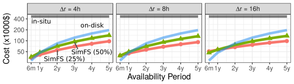
Figure 12: Data availability cost for different availability periods.

Simulation Data Availability Period Figure 1 shows the cost of supporting 100 forward-in-time analyses executed over different $\Delta t$s (x-axis) with a $50\%$ overlap. SimFS is configured with a storage cache of size equal to the $25\%$ of the total simulation data volume and a restart interval of $\Delta r=8h$ The in-situ cost does not depend on $\Delta t$ since no data needs to be permanently stored. On the contrary, the on-disk solution stores all the simulation data, avoiding re-simulations. SimFS combines the two approaches: while it requires less storage than on-disk, it needs to pay the cost of re-simulating the missing files. The cost-effectiveness of SimFS depends on the total amount of analyses and $\Delta t$: if the data is analyzed by many applications in a short availability period, then on-disk is a better because, once the data is stored, the analysis is virtually free. Otherwise, if the same analyses are spread over a very long time period, then in-situ is more cost-effective because no (time-dependent) storage cost is paid. SimFS is designed to be cost-effective for scenarios in between these two extremes: it does not store the full simulation data, saving on the storage cost, but uses the storage to cache simulation data, saving on the compute cost for recurrent analysis.

Figure 12 shows this experiment varying the SimFS cache size ($25\%$ and $50\%$) and $\Delta r$. While larger restart intervals require less storage for the restart files, they lead to an increase of the SimFS cost for short $\Delta t$s: in these cases, the cost is sensible to the re-simulations and larger $\Delta r$ can lead to more capacity misses (it acts as cache block size, see Sec. II-A).

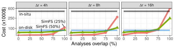
Figure 13: Data availability cost for different analyses overlaps.

Analyses Execution Overlap Figure 13 shows the same experiment but varying the analyses overlaps and fixing $\Delta t=2y$ (other settings are unchanged). Higher overlap lead to more interleaved analyses: since they access different output steps, this leads to a lower temporal locality, hence to an increased number of misses. This is amplified when using larger $\Delta r$ since this can increase the number of capacity misses.

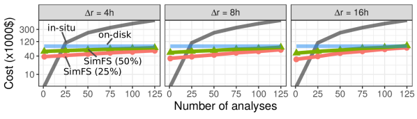
Figure 14: Data availability cost for different numbers of analyses.

Total Number of Analyses Figure 14 shows the cost when varying the number of analyses executing during $\Delta t$. We fix the availability period to $\Delta t=2y$ and the analyses overlap at $50\%$. Independently from the restart interval and cache size, SimFS cannot beat in-situ when the number of analyses is less than 20: the cost of the initial simulation plus the storage of restarts and cached output steps is higher than the cost of coupling each analysis with its own simulation. However, when increasing the number of analyses, in-situ becomes more expensive since no data is shared among the different analyses.

V-B Discussion

These cost models allow to estimate the data availability costs for both HPC and cloud infrastructures: Figure 15a is a heatmap showing the ratio between the minimum cost between ondisk and in-situ and the SimFS cost, for different storage and compute costs configurations (i.e., the darker the color, the higher the ratio). We use the same scenario and parameters of Sec. V-A, focusing on the case with 100 analyses, 50% overlap, $3y$ of data availability, and the SimFS cache set up to the 25% of the total simulation data volume. On the heatmap we show two real-world datapoints: the Microsoft Azure configuration of Sec. V-A, and the Piz Daint compute and storage costs. The Piz Daint costs are derived from the CSCS cost catalog [18].

To determine the cost-effectiveness of SimFS w.r.t. other solutions, one needs to know, among the others, the type of analyses performed during a given data availability period. While this is a limiting factor of this cost model, we plan to use online information to dynamically adapt the SimFS configuration (e.g., cache size, restart interval) in a future work. Figure 15b and Figure 15c show the potential effects of these changes (same configuration of above). They report the re-simulation cost and time as function of the storage space reserved for restart files and for different cache sizes, respectively. They show that (1) the restart interval and the cache size influence cost and compute time, and (2) the reduced compute time due to having a bigger cache might not be justified by the higher cost: e.g., for $\Delta r=8$, a 50% cache size reduces the compute time of 20% but increases the cost of 25%.

Figure 15: (a) SimFS cost-effectiveness heatmap; (b) Cost over space; (c) Re-simulation time vs Space.

VI Evaluation

The benchmarks presented in this section are executed on Piz Daint, a Cray XC50 system. The compute nodes are equipped with two Intel Xeon E5-2695 @ 2.10GHz with eighteen cores each. The system is interconnected with Cray’s Aries network and uses Lustre [19] as parallel file system. The measurements are taken by DVLib via the LibLSB library [20].

COSMO is a non-hydrostatic local area atmospheric model used for both operational numerical weather prediction and long-term climate simulation [21, 22]. In this benchmark we study the strong scalability of the system composed by a virtualized COSMO simulation, SimFS, and a (sequential) analysis. The analysis computes mean and variance of a 1-D field of the simulation output steps. The simulation proceeds in one-minute timesteps, producing one output step every five minutes ($\Delta d=5$) and one restart file every hour ($\Delta r=60$).

The simulation context is configured to use the optimal number of compute nodes ($P=100$) as default, hence the prefetching strategy (2) (see Sec. IV-B) is applied. Let us define $s_{\text{max}}$ as the maximum number of re-simulations that can be run at the same time by SimFS. This parameter limits the amount of computing resources that SimFS can employ but it also limits the effectiveness of the prefetching strategies: once $s_{\text{max}}$ simulations are running, SimFS will not be able to prefetch new ones to mask their restart latencies, delaying the analysis.

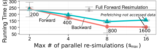
Figure 16: Strong scalability of analyses accessing virtualized COSMO data. The data points are annotated with the number of used compute nodes.

Figure 16 shows the analysis completion time as function of $s_{\text{max}}$. We report the completion times of a forward and backward analysis accessing the same output steps but in different order. For comparison, we also report the time of a full forward simulation, that is the time needed by a single simulation to produce the same sequence of output steps. The analysis tool completion time scales up to a factor of $2.4$x w.r.t. the full forward re-simulation when $s_{\text{max}}=8$. The backward simulation shows a slightly worse scalability (up to a factor of $1.6$x): this is because the first access of this analysis is served after the simulation of an entire restart interval, delaying the prefetching activity (see Figure 10). At $s_{\text{max}}=16$ prefetching does not bring any further benefit because the prefetched simulations produce output steps that are not accessed by the analysis, which terminates after analyzing the first $6$ hours of the simulated data (i.e., $72$ output steps).

Figure 17: Prefetching COSMO simulations under different restart latencies and analysis lengths.

With these settings, the simulation produces an output step every $\tau_{\text{sim}}=3s$ on average and has restart latency of $\alpha_{\text{sim}}=13s$. The reported $\alpha_{\text{sim}}$ does not include the re-simulation jobs queuing time. To study the effects the re-simulation jobs queuing times on the prefetching effectiveness we simulate the analysis running time over different restart latencies (now including the job queueing time) and analysis lengths ($m$). We use a synthetic simulator that can be configured to produce output steps at a given rate (i.e., $1/\tau_{\text{sim}}$) and after a given restart latency. We use the same $\tau_{\text{sim}}$ of the COSMO simulation described above, but we vary the restart latency in order to simulate different job queuing times. Figure 17 shows the results for $s_{\text{max}}=8$. As discussed in Sec. IV-C1, when the restart latency is much higher than the time needed to produce the output steps accessed by the analysis, the analysis running time converges to the prefetching warm-up time and no benefits arise from the prefetching of multiple simulations in parallel (i.e., strategy (2)). The warm-up time is a factor of two higher than $T_{\text{single}}$, which is the time of a single simulation serving all the analysis accesses: $T_{\text{single}}=\alpha_{\text{sim}}+m\cdot\tau_{\text{sim}}$. This bounds the overhead that SimFS can introduce w.r.t. an in-situ analysis. We also report a simple lower bound for this prefetching strategy, $T_{\text{lower}}$, that is the given by the restart latency plus the time of serving all the output steps requested by the analysis using $s_{\text{max}}$ simulations in parallel: $T_{\text{lower}}=\alpha_{\text{sim}}+m\cdot\frac{\tau_{\text{sim}}}{s_{\text{max}}}$.

FLASH is a multiphysics simulation framework [23]. In this experiment we virtualize a Sedov simulation [24] which involves the evolution of a blast wave from an initial pressure perturbation in an otherwise homogeneous medium [25]. The simulation is configured to have $32^{3}$ cells per block (one block per core). We simulate the first second of the blast wave evolution. The simulation proceeds in $0.005$s timesteps and produces one output step at each timestep ($\Delta d=1$) and one restart file every $0.1$s ($\Delta r=20$). The analysis computes mean and variance of the velocity field. With these settings, we measure $\tau_{\text{sim}}=14s$ and $\alpha_{\text{sim}}=7s$ (not including the re-simulation jobs queuing time).

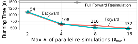
Figure 18: Strong scalability of analyses accessing virtualized FLASH data. The data points are annotated with the number of used compute nodes.

Figure 18 shows the analysis time over of $s_{\text{max}}$: it scales up to a factor of $3$x when $s_{\text{max}}=16$. Differently from the COSMO case, here forward and backward analysis show the same behavior: This is due to the higher restart steps frequency of this configuration that reduces the time needed to complete the resimulation serving the first miss.

Figure 19 shows the analysis running time for different restart latencies and analysis lengths, fixing $s_{\text{max}}=8$. We configure the synthetic simulator to run as the FLASH configuration described above. Differently from the COSMO study (i.e., Figure 17), here the prefetching strategy is more effective: this is due to the number of output steps analyzed and the higher $\tau_{\text{sim}}$, that better composate the prefetching warm-up time $T_{\text{pre}}$. This figure shows also how, in some cases, increasing the restart latency leads to a reduction of the analysis running time (e.g., tile with $m=400$, between $\alpha_{\text{sim}}=100s$ and $\alpha_{\text{sim}}=500s$). This is explained by the fact that, due to the higher restart latency, SimFS determines a longer re-simulation length $n$ (see Sec. IV-B1), starting the simulation of the next $s_{\text{max}}\cdot n$ output steps at each prefetch step. The new block of simulations may now simulate enough output steps to satisfy the remaining analysis, avoiding the analysis to pay a new restart latency caused by the $s_{\text{max}}$ parameter.

Figure 19: Prefetching FLASH simulations under different restart latencies and analysis lengths.

VII Related Work

In-situ and on-disk are widely used solutions for simulation data analysis. In-situ avoids to store the data on disk by performing part of the analysis (or filtering) directly at the simulation site [26, 27], or during the data staging phase (i.e., in transit) [28], or at the analysis tool site bypassing the parallel file system (i.e., loosely coupled in-situ) [29]. In all the cases, the analysis is performed as the data is simulated and independent analysis applications have to run in tandem with their own simulation. On-disk analysis is orthogonal to in-situ: here the analysis accesses the data that is stored on disk, without dealing with the simulation process. SimFS enables a tradeoff between these two approaches, which are at the two ends of the storage requirements spectrum. In fact, virtualizing the simulation output allows to adjust the storage requirements while offering to the analysis the same file abstraction of the on-disk solution.

SimFS implements cache replacement strategies that are based on data locality or data access cost. Cost-based schemes are well studied in literature: Park et al. [30] consider different costs for writing back dirty entries to flash memory disks and prioritize the eviction of the (cheaper) non-dirty pages. However, this binary cost approach is not suitable in our context where the output steps have costs linear in their distance from the previous closest restart file. Jeong et al. [14, 31] propose a collection of cost-aware algorithms for NUMA architectures with variable costs. Our cost-based replacement schemes build on top of their algorithms (i.e., BCL and DCL).

VIII Summary

We argue that storing the full simulation output is not cost-effective because the ever growing availability of computing power enables multi-petabyte simulation runs. SimFS virtualizes the simulation data: the data is only partially stored and accesses to missing data are served by restarting simulations. The analysis applications can be transparently interfaced to SimFS or made virtualization-aware by using the SimFS APIs.

All in all, SimFS introduces a new simulation data analysis paradigm that relaxes the storage requirements and offers a viable path towards exa-scale simulations. SimFS can be downloaded at:

https://github.com/spcl/SimFS

References

- [1] M. Grawinkel et al., “Analysis of the ECMWF Storage Landscape,” in Proc. of the 13th USENIX Conf. on File and Storage Technologies, ser. FAST’15. Berkeley, CA, USA: USENIX Association, 2015. [Online]. Available: http://dl.acm.org/citation.cfm?id=2750482.2750484
- [2] D. Potter et al., “PKDGRAV3: Beyond Trillion Particle Cosmological Simulations for the Next Era of Galaxy Surveys,” arXiv preprint arXiv:1609.08621, 2016.
- [3] M. Bernyk et al., “The theoretical astrophysical observatory: Cloud-based mock galaxy catalogs,” The Astr. Journal Supplement Series, vol. 223, no. 1, p. 9, 2016.
- [4] A. Ragagnin et al., “An online theoretical virtual observatory for hydrodynamical, cosmological simulations,” arXiv preprint arXiv:1612.06380, 2016.
- [5] E. Winsberg, Science in the age of computer simulation. University of Chicago Press, 2010.
- [6] M. Folk et al., “HDF5: A file format and I/O library for high performance computing applications,” in Proc. of Supercomputing, vol. 99, 1999.
- [7] R. K. Rew and G. P. Davis, “The unidata netCDF: Software for scientific data access,” in Sixth Int. Conf. on Interactive Information and Processing Systems for Meteorology, Oceanography, and Hydrology, 1990.
- [8] J. F. Lofstead et al., “Flexible IO and integration for scientific codes through the adaptable IO system (ADIOS),” in Proc. of the 6th Int. Workshop on Challenges of Large Applications in Distributed Environments. ACM, 2008.
- [9] A. Arteaga, O. Fuhrer, and T. Hoefler, “Designing Bit-Reproducible Portable High-Performance Applications,” in Proc. of the 28th IEEE Int. Parallel and Distributed Processing Symp. (IPDPS). IEEE Computer Society, Apr. 2014.
- [10] I. Müller et al., “Reproducible Floating-Point Aggregation in RDBMSs,” arXiv preprint arXiv:1802.09883, 2018.
- [11] M. D. Hill, “21st Century Computer Architecture,” SIGPLAN Not., Feb. 2014. [Online]. Available: http://doi.acm.org/10.1145/2692916.2558890
- [12] S. Jiang and X. Zhang, “LIRS: an efficient low inter-reference recency set replacement policy to improve buffer cache performance,” ACM SIGMETRICS Performance Evaluation Review, 2002.
- [13] N. Megiddo and D. S. Modha, “ARC: A Self-Tuning, Low Overhead Replacement Cache,” in FAST, 2003.
- [14] J. Jeong and M. Dubois, “Cache replacement algorithms with nonuniform miss costs,” IEEE Transactions on Computers, vol. 55, no. 4, pp. 353–365, 2006.
- [15] “Microsoft Azure,” https://azure.microsoft.com, 2018, accessed: 2018/04.
- [16] “Microsoft Azure VM Pricing,” https://azure.microsoft.com/en-us/pricing/details/virtual-machines/linux/, 2018, accessed: 2018/04.
- [17] “Microsoft Azure Storage Pricing,” https://azure.microsoft.com/en-us/pricing/details/storage/files/, 2018, accessed: 2018/04.
- [18] “CSCS2Go,” https://2go.cscs.ch/home/, 2018, accessed: 2018/12.
- [19] P. J. Braam et al., “The Lustre storage architecture,” 2004.
- [20] T. Hoefler and R. Belli, “Scientific Benchmarking of Parallel Computing Systems.” ACM, Nov. 2015, pp. 73:1–73:12, proc. of the Int. Conf. for High Performance Computing, Networking, Storage and Analysis (SC15).
- [21] Consortium for small-scale modeling, “Web page,” 1998, accessed: 2017/03. [Online]. Available: http://www.cosmo-model.org
- [22] O. Fuhrer et al., “Near-global climate simulation at 1km resolution: establishing a performance baseline on 4888 gpus with cosmo 5.0,” Geoscientific Model Development Discussions, 2017.
- [23] B. Fryxell et al., “FLASH: An Adaptive Mesh Hydrodynamics Code for Modeling Astrophysical Thermonuclear Flashes,” The Astr. Journal Supplement Series, vol. 131, no. 1, p. 273, 2000. [Online]. Available: http://stacks.iop.org/0067-0049/131/i=1/a=273
- [24] L. I. Sedov, Similarity and Dimensional Methods in Mechanics, 1959.
- [25] F. C. for Computational Science University of Chicago, “Flash user’s guide version 4.4,” 2016, accessed: 2017-03-17. [Online]. Available: http://flash.uchicago.edu/site/flashcode/user_support/flash4_ug_4p4.pdf
- [26] N. Richart et al., “Toward a computational steering environment for legacy coupled simulations,” in Sixth Int. Symp. on Par. and Distr. Comp., 2007. (ISPDC’07). IEEE, 2007.
- [27] F. Zhang et al., “Enabling in-situ execution of coupled scientific workflow on multi-core platform,” in 26th Int. Par. & Distr. Processing Symp. (IPDPS). IEEE, 2012.
- [28] J. C. Bennett et al., “Combining in-situ and in-transit processing to enable extreme-scale scientific analysis,” in Int. Conf. for High Performance Computing, Networking, Storage and Analysis (SC), 2012. IEEE, 2012, pp. 1–9.
- [29] H. Yu et al., “In situ visualization for large-scale combustion simulations,” IEEE computer graphics and applications, vol. 30, no. 3, 2010.
- [30] S.-y. Park et al., “CFLRU: a replacement algorithm for flash memory,” in Proc. of the 2006 Int. Conf. on Compilers, Architecture and Synthesis for Embedded Systems. ACM, 2006.
- [31] J. Jeong and M. Dubois, “Cost-sensitive cache replacement algorithms,” in Proc. The Ninth Int. Symp. on High Performance Architecture. IEEE, 2003.