Spin dynamics of a millisecond pulsar orbiting closely around a massive black hole

Abstract

We investigate the spin dynamics of a msp in a tightly bounded orbit around a massive black hole. These binaries are progenitors of the emri and imri gravitational wave events. The mpd formulation is used to determine the orbital motion and spin modulation and evolution. We show that the msp will not be confined in a planar Keplerian orbit and its spin will exhibit precession and nutation induced by spin-orbit coupling and spin-curvature interaction. These spin and orbital behaviours will manifest observationally in the temporal variations in the msp’s pulsed emission and, with certain geometries, in the self-occultation of the pulsar’s emitting poles. Radio pulsar timing observations will be able to detect such signatures. These emrb and imrb are also strong gravitational wave sources. Combining radio pulsar timing and gravitational wave observations will allow us to determine the dynamics of these systems in high precision and hence the subtle behaviours of spinning masses in strong gravity.

1 Introduction

The gravitational wave events, e.g. GW150914 (Abbott et al., 2016) and GW170608 (Abbott et al., 2017b), etc, detected by ligo provide strong support for Einstein’s theory of gravity, i.e. general relativity (GR) and evidence for astrophysical black holes. Although GR has passed a variety of tests in the weak field and strong field regimes, there are still issues within it that require further clarification (see e.g. Beiglböck, 1967; Costa & Natário, 2014). Among them is the dynamics of spinning objects, in particular, regarding how spin interacts with curved space-time (Plyatsko, 1998; Iorio, 2012; Plyatsko & Fenyk, 2016) and what the corresponding observable signatures are.

Binary systems containing an msp orbiting around a massive black hole (of $10^{3}-10^{6}\;\!{\rm M}_{\odot}$) are particularly useful for the study of spin-curvature interaction in GR. With the large mass ratio between the black hole and the msp, the neutron star can be treated as a point test particle. The space-time is practically stationary, provided solely by the black hole. These allow us to construct models that are simple enough to be mathematically tractable yet sufficient for capturing the essences of the physics and its subtle complexity. Depending on the mass of the black hole, the binary systems can be split explicitly into emrb (for black holes between $10^{5}-10^{6}\;\!{\rm M}_{\odot}$) and imrb (for black holes between $10^{3}-10^{4}\;\!{\rm M}_{\odot}$), which correspond to different astrophysical systems. emrb/imrb are progenitors of the emri/imri systems. They are major classes of gravitational wave sources expected to be detected by lisa (see e.g. Amaro-Seoane et al., 2007). The presence of an msp guarantees the electromagnetic counterparts of these emrb/imrb and the subsequent emri/imri gravitational wave events. With high-precision radio timing observations the spin and orbital dynamics of the msp can be investigated independently, complimentary to the direct gravitational wave observations.

emrb and imrb systems are astronomically important in their own right. How emrb were formed and how their progenitors had evolved to such configuration are interesting questions to be answered. A possibility is that compact msp - black hole binaries were formed in very dense stellar environments (Merritt et al., 2011; Clausen et al., 2014), e.g. the central region of a large stellar spheroid, such as the core of a compact spheroidal galaxy, through sequences of stellar interactions. Another possibility is that they were produced at the centre of a small elliptical or a Milky-Way-like spiral galaxy when an msp is captured by the nuclear black hole. imrb systems could also be formed in dense environments where an intermediate-mass black hole capture an msp. Globular clusters are known to host a large population of pulsars, in particular, msp (see e.g. Lorimer, 2008). Neutron stars are the more massive stars in the globular clusters and they would sink to the core of their host globular clusters due to dynamical friction. If the globular cluster has an intermediate-mass nuclear black hole, an imrb system would, therefore, be formed. We will discuss the possibility of these events further in §4.2.

Spinning neutron stars or spinning neutron-star binaries revolving around a massive black hole had been investigated in various astrophysical contexts (e.g. Remmen & Wu, 2013; Singh et al., 2014; Rosa, 2015; Saxton et al., 2016). Most of these studies put focus on the orbital dynamics of the neutron star or the neutron-star binaries. This work will extend the previous investigations to the dynamics of the neutron star’s spin when orbiting around a massive black hole in the presence of spin-orbit and spin-curvature couplings. We determine on the observational signatures as diagnosis and discuss their astrophysical and physical implications. The paper is organised as follows. In §2 we present the formulation for the equation, and in §3 we show the results for systems with parameters relevant to astrophysics and to future pulsar timing observations and gravitational wave experiment. Discussions on the astrophysics and physics implications will be in §4 and a summary in §5.

2 Equations of motion

We adopt a $[\,-\;\!+\;\!+\;\!+\,]$ signature for the metric and a natural unit system, in which the gravitational constant $G$ and the speed of light $c$ are unity ($G=c=1$). The msp, a neutron star with mass $m\;\!(=M_{\rm ns})$ and radius $R_{\rm ns}$, orbits around a black hole of mass $M\;\!(=M_{\rm bh})$. The black hole has a Schwarzschild radius $R_{\rm sch}=2M$, and its rotation is specified by the spin parameter $a$, with $a/M=1$ corresponding to a maximally rotating Kerr black hole and $a/M=0$ corresponding to a non-rotating (Schwarzschild) black hole. The orbital separation between the msp and the black hole, $r$, is sufficiently large such that $r>M\gg R_{\rm ns}>m$. The space-time is stationary, determined by the black hole’s gravity and rotation, i.e. a Kerr space-time.

The space-time interval, in the Boyer-Lindquist coordinates, is therefore given by

$$-{\rm d}\tau^{2}= -\left(1-\frac{2Mr}{\Sigma}\right){\rm d}t^{2}-\frac{4aMr\sin^{2}\theta}{\Sigma}\;\!{\rm d}t\;\!{\rm d}\phi$$ (1)

$$+\frac{\Sigma}{\Delta}\;\!{\rm d}r^{2}+\Sigma\;\!{\rm d}\theta^{2}+\left(r^{2}+a^{2}+\frac{2a^{2}Mr\sin^{2}\theta}{\Sigma}\right)$$

$$\times\sin^{2}\theta\;\!{\rm d}\phi^{2}\ ,$$

where $\Sigma=r^{2}+a^{2}\cos^{2}\theta$, $\Delta=r^{2}-2Mr+a^{2}$ and $(r,\theta,\phi)$ represents the spatial 3-vector in the (pseudo-)spherical polar coordinates with the black-hole centre as the origin. The motion of the msp, in the approximation as a particle-like object, is determined by the continuity equation

$$T^{\mu\nu}{}_{;\mu}=0\ ,$$ (2)

where the covariant derivative is taken with respect to the background spacetime. For a spinning particle with 4-momentum $p^{\mu}$ and spin-tensor $s^{\mu\nu}$, the continuity equation can be simplified to the mpd equations:

$$\frac{{\rm D}p^{\mu}}{{\rm d}\tau}=-\frac{1}{2}\;\!{R^{\mu}}_{\nu\alpha\beta}u^{\nu}s^{\alpha\beta}\ ;$$ (3)

$$\frac{{\rm D}s^{\mu\nu}}{{\rm d}\tau}=p^{\mu}u^{\nu}-p^{\nu}u^{\mu}$$ (4)

(see Mashhoon & Singh, 2006; Plyatsko et al., 2011), where $u^{\mu}={\rm d}x^{\mu}/{\rm d}\tau$ is the 4-velocity of the centre of mass. We have omitted the Dixon force ${\cal F}^{\mu}$ in the momentum evolutionary equation and the Dixon torque ${\cal T}^{\mu\nu}$ in the spin evolutionary equation (cf. Singh et al., 2014). They are arisen from the interaction of the quadrupole and higher-order mass moments of the spinning object with the gravitational field and therefore absent in the point-mass approximation that we have adopted for the msp.

To close the mpd equation, a spin supplementary condition is required. We consider the Tulczyjew-Dixon (TD) condition (see Tulczyjew, 1959; Deriglazov & Ramírez, 2017), where

$$s^{\mu\nu}p_{\nu}=0\ .$$ (5)

This, together with the point-mass approximation, ensures that the mass of the msp, given by

$$m=\sqrt{-\;\!p^{\mu}p_{\mu}\;\!}\ ,$$ (6)

is a constant of motion. The spin vector $s_{\mu}$ of the msp is obtained by the contraction of the spin tensor $s^{\mu\nu}$:

$$s_{\mu}=-\frac{1}{2m}\;\!\epsilon_{\mu\nu\alpha\beta}p^{\nu}s^{\alpha\beta}\ ;$$ (7)

$$s^{\mu\nu}=\frac{1}{m}\;\!\epsilon^{\mu\nu\alpha\beta}p_{\alpha}s_{\beta}\ ,$$ (8)

with Levi-Civita tensor $\epsilon_{\mu\nu\alpha\beta}=\sqrt{-\;\!g\;\!}\;\!\sigma_{\mu\nu\alpha\beta}$ adopting the $\sigma_{0123}=+1$ permutation. Contraction of the spin vector gives the scalar

$$s^{2}=s^{\mu}s_{\mu}=\frac{1}{2}\;\!s^{\mu\nu}s_{\mu\nu}\ ,$$ (9)

which is a constant of motion.

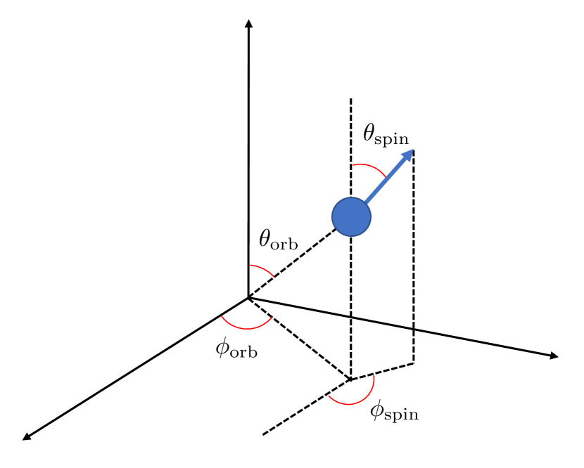
Figure 1: The geometry of the system. The orbital angles $\phi_{\rm orb}$ and $\theta_{\rm orb}$ are defined with respect to the (pseudo-)spherical polar coordinate with respect to the centre of the black hole. The spin angles $\phi_{\rm spin}$ and $\theta_{\rm spin}$ are defined on a Cartesian coordinate in the msp’s local tetrad frame.

In the regime where the Møller radius of the msp (i.e., a neutron star)

$$r_{\rm M}=\frac{s}{m}\ll r\ ,$$ (10)

the dipole-dipole interaction and the higher-order multipole interactions, which are much weaker than the pole-dipole interaction, can be ignored. Thus,

$$\left(\frac{p^{\mu}}{m}-u^{\mu}\right)\sim\frac{M\;\!{{r_{\rm M}}^{2}}}{r^{3}}\ll 1\ ,$$ (11)

and the approximation scheme proposed by Chicone et al. (2005) is applicable. With $p^{\mu}\approx mu^{\mu}$, the mpd equations are reduced to

$$\frac{{\rm D}u^{\mu}}{{\rm d}\tau}=-\frac{1}{2m}\;\!{R^{\mu}}_{\nu\alpha\beta}u^{\nu}s^{\alpha\beta}\ ;$$ (12)

$$\frac{{\rm D}s^{\mu\nu}}{{\rm d}\tau}\approx 0\ ,$$ (13)

and the closure condition becomes

$$s^{\mu\nu}u_{\nu}\approx 0$$ (14)

(Chicone et al., 2005; Mashhoon & Singh, 2006). This is essentially the Frenkel-Mathisson-Pirani (FMP) condition (Frenkel, 1926; Mathisson, 1937; Costa & Natário, 2014; Costa et al., 2018) .

To investigate the difference between the cases with and without consideration of spin-curvature coupling, we introduce a parameter switch $\lambda$ into the mpd equations as in Singh et al. (2014) (see also Singh, 2005):

$$\frac{{\rm d}p^{\alpha}}{{\rm d}\tau}=-{\Gamma^{\alpha}}_{\mu\nu}p^{\mu}u^{\nu}+\lambda\left(\frac{1}{2m}{R^{\alpha}}_{\beta\rho\sigma}{\epsilon^{\beta\sigma}}_{\mu\nu}s^{\mu}p^{\nu}u^{\beta}\right)\ ;$$ (15)

$$\frac{{\rm d}s^{\alpha}}{{\rm d}\tau}=-{\Gamma^{\alpha}}_{\mu\nu}s^{\mu}u^{\nu}+\lambda\left(\frac{1}{2m^{3}}R_{\gamma\beta\rho\sigma}{\epsilon^{\beta\sigma}}_{\mu\nu}s^{\mu}p^{\nu}s^{\gamma}u^{\beta}\right)p^{\alpha}\ ;$$ (16)

$$\frac{{\rm d}x^{\alpha}}{{\rm d}\tau}=u^{\alpha}=-\frac{p^{\delta}u_{\delta}}{m^{2}}\left(p^{\alpha}+\frac{1}{2}\;\!\frac{\lambda(s^{\alpha\beta}R_{\beta\gamma\mu\nu}p^{\gamma}s^{\mu\nu})}{m^{2}+\lambda(R_{\mu\nu\rho\sigma}s^{\mu\nu}s^{\beta\sigma}/4)}\right)\ .$$ (17)

Spin-curvature coupling is included when $\lambda=1$, and excluded when $\lambda=0$. In this formula, the spin 4-vector is Fermi-Walker transported along the worldline of the centre-of-motion of the msp.

3 Spin and orbit modulation of the millisecond pulsar

We adopt a neutron-star mass $m=1.5~{}{\rm M}_{\odot}$. The msp spin period $P_{\rm s}$ is taken to be $1~{}{\rm ms}$ (with spin $s=0.3787m^{2}$ throught out this paper) , for the extremely fast rotating msp (see Papitto et al., 2014; Özel & Freire, 2016, for the period distributions of msp). The massive black hole (MBH) is taken to have mass $M=10^{3}$, $10^{4}$ and $10^{5}\;\!{\rm M}_{\odot}$, and the spin parameter $a/M=0$, $\pm 0.5$ and $\pm 0.99$. The orbit of the msp around the black hole is bounded, with $``+"$ and $``-"$ signs in $a/M$ corresponding to the black hole in a prograde and a retrograde rotation with respect to the orbital motion of the msp. The semi-major axis $r$ of the orbit of msp, defined as the mean of minimum and maximum distances between the msp and black hole, is chosen to be 20, 50 and $100\;\!M$. The eccentricity $e$ of the orbit is calculated using the method described in Appendix A. It has values ranging between 0 and 0.6 . The initial orientation of the msp’s spin axis is set to be $0^{\circ}$, $45^{\circ}$ and $90^{\circ}$ with respect to the initial Newtonian orbital angular momentum. The system geometry is shown in Fig. 1.

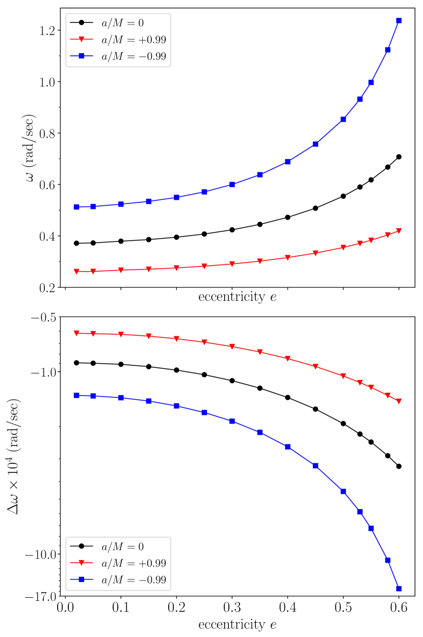
Figure 2: (Figure is updated) The upper panel shows the rate of periastron advance as a function of eccentricity $e$ in the pure geodesic case. The lower panel shows the corrections to the rate of periastron advance due to spin-orbit and spin-curvature couplings, for an msp with period $1~{}{\rm ms}$. The semi-major axis of the orbit of the msp is set to be $r=20M$, and the mass of the central black hole $10^{3}\;\!{\rm M}_{\odot}$. The blue, black, red lines correspond to the cases of the black-hole spin $a/M=-0.99$ (retrograde with respect to the msp orbit), $0$, and $0.99$ (prograde with respect to the msp orbit) respectively. The spin of the msp is parallel to the orbital angular momentum initially. The rate of geodetic periastron advance in the upper panel is decreased by $10$ and $10^{2}$ times for central black holes with $10^{4}\;\!{\rm M}_{\odot}$ and $10^{5}\;\!{\rm M}_{\odot}$ respectively, while the correction to the rate due to the msp’s spin is decreased by $10^{2}$ and $10^{4}$ times respectively. Notice that the y-axis of the lower panel is in log scale, which shows that the effects of spin-orbit and spin-curvature couplings are greatly enhanced in the highly eccentric cases.

3.1 Results

In the mpd formulation, the msp’s orbital motion and spin evolution are interdependent (see Eq. 17). Fig. 2 shows the rate of the periastron advancement as a function of the orbital eccentricity ($e$) expected for geodesic motion (top panel) and the correction to the rate when spin-orbit and spin-curvature couplings are considered (bottom panel). The precession rate of the msp’s orbit is generally faster for $a/M<0$ than for $a/M>0$. The precession is determined by several mechanisms, among them the strongest is due to geodesic motion, similar to that in Mercury when it revolves around the Sun. Another one is due to the Lense-Thirring effect, arisen from the black hole’s rotation. This effect is clearly visible when comparing the rates for non-zero $a/M$ with that for $a/M=0$. The precession is also contributed by the interaction between the msp’s spin with the msp’s orbit motion and with the space-time curvature induced by the black hole’s gravity. Note that for the system parameters considered in this work, the advancement of the orbital precession is comparable (see top panel, Fig. 2) to the angular velocity of the msp’s orbital motion, which is about $\sim 2~{}{\rm rad~{}s}^{-1}$ (for $M=10^{3}\;\!{\rm M}_{\odot}$). Perturbation methods, in particular those assuming a quasi-circular orbit, are therefore not always applicable when determining the msp’s orbital dynamics for systems with non-zero eccentricities.

In a classical eccentric binary system, orbital precession is usually caused by tidal interactions between the components and/or the presence of quadrupole and/or higher-order multipole mass moments in the components. Here we have demonstrated the presence of the well-known orbital precession due to general relativistic effects, such effects have been studied extensively in literature (see e.g. Kidder, 1995; Ruangsri et al., 2016). One of the consequence is that the orbital precession is enhanced. This additional acceleration can be illustrated in terms of a 1PN (first-order post-Newtonian) correction for a parametrised Keplerian binary system (Damour & Deruelle, 1985, 1986).

The strength of spin-orbit interaction in the system may be characterised in terms of an effective interaction

$$\chi_{\rm eff}=\frac{1}{(M+m)}\left(\frac{\boldsymbol{s}}{m}+\frac{\boldsymbol{S}_{\rm MBH}}{M}\right)\cdot\boldsymbol{\hat{L}}\ ,$$ (18)

where $\boldsymbol{s}$ and $\boldsymbol{S}_{\rm MBH}$ are the spin vectors of the msp and the massive black hole respectively and $\boldsymbol{\hat{L}}$ is the unit directional vector of the msp’s orbital angular momentum $\boldsymbol{L}$. Here, $\boldsymbol{S}_{\rm MBH}$ is related to the spin parameter by $\boldsymbol{S}_{\rm MBH}=aM\boldsymbol{\hat{S}}_{\rm MBH}$. (Hereafter, unless otherwise stated, $\boldsymbol{\hat{x}}$ denotes that the unit directional vector of a vector $\boldsymbol{x}$.) For a black hole and an msp that have the same value of dimensionless spin $a/M$ and $s/m^{2}$, the effects of msp’s spin on the orbital dynamics and spin dynamics are scaled with the factor $m/M$. The value of dimensionless spin of msp depends on its rotational period and inner structure. From the observational perspective, the pulsed signals allow us to determine the rotational period of the msp, while the strength of spin-orbit couplings depends on the dimensionless spin of the msp. Therefore, by measuring such a binary system, we can not only probe the space time structure of the MBH, but also achieve two independent measurements of the msp’s rotation period and moment of inertia, which potentially provide us clues about the inner structure of the msp.

Fig. 3 shows the corresponding difference of $u^{0}$, the ratio of the coordinate time ${{\rm d}t}$ and the proper time ${{\rm d}\tau}$ of the msp. The msp serves as an accurate clock . Therefore, ${{\rm d}t}/{{\rm d}\tau}$ can be directly measured if we know the intrinsic rotational period of the msp.

We consider a quasi-circular orbit approximation and determine the different effects on $u^{0}$ by expanding the analytic formula of $u^{0}$ for geodesic orbits with respect to the eccentricity $e$ and the Post-Newtonian (PN) factor $M/r$. As no assumption is made for the spins of the black hole and the msp, the expression that we obtain is valid for the extremely rotating black hole (with $a/M=\pm 0.99$) and fast spinning msp.

The details of the calculations are shown in Appendix B. The estimated values of $\Delta u^{0}$ due to each factor are shown in Table. 1. These results are consistent with the those shown in the upper and middle panels of Fig. 3.

For an msp with a highly eccentric orbit, only the corrections due to the coupling of msp’s spin to orbital angular momentum are shown in Fig. 3 (lower panel). The corrections are much greater than the results estimated by using the linear approximation in Appendix B, mainly due to the breaking down of Taylor expansion of $u^{0}$ with respect to the eccentricity $e$. In general, a correction of about $\sim 20\;\!{\rm ns}$ arises within a duration of $\sim 10-1000~{}{\rm sec}$, for black hole with masses between $10^{3}-10^{5}\;\!{\rm M}_{\odot}$.

Effect	scale	$\Delta\frac{{\rm d}t}{{\rm d}\tau}$	${\Delta\frac{{\rm d}t}{{\rm d}\tau}}/{T_{\rm orb}}$
GR	$\frac{3}{2}\frac{M}{r}$	$0.075~{}{\rm ms}$	$2.7\times 10^{-5}$
Eccentricity	$2e\frac{M}{r}$	$2~{}\mu{\rm s}$	$7.2\times 10^{-7}$
MBH’s spin	$3\frac{a}{M}(\frac{M}{r})^{5/2}$	$1.66~{}\mu{\rm s}$	$6.0\times 10^{-7}$
msp’s spin	$2\delta e\frac{M}{r}+\frac{3}{2}\frac{M}{r}\frac{\delta r}{r}$	$3.12~{}{\rm ns}$	$1.1\times 10^{-9}$

Table 1: The correction to the time component of msp’s 4-velocity (i.e. $u^{0}$), which is the ratio of coordinate time ${{\rm d}t}$ and proper time ${{\rm d}\tau}$, by different factors for circular and quasi-circular orbits. The formula are calculated in Appendix B, and only leading orders are shown in the table for order estimation. Here we take $m=1.5~{}{\rm M}_{\odot}$, $M=10^{3}~{}{\rm M}_{\odot}$, semi-major axis $r=20M$, $e=0.02$, $a/M=\pm 0.99$ and $s=0.4m^{2}$ for an example. For the effect of eccentricity, ${\rm d}t/{\rm d}\tau$ is evaluated at either periastron or apastron, and is compared to circular orbit with the same semi-major axis. For the effect of MBH’s spin, ${\rm d}t/{\rm d}\tau$ is evaluated for circular orbit around spinning MBH, and compared to circular orbit with the same radius around non-spinning MBH. When we include the msp’s spin, the eccentricity is perturbed by $\delta e\sim 2\times 10^{-5}$, while the semi-major axis is perturbed by $\delta r=3\times 10^{-4}M$, leading to a perturbation of about $3.12~{}{\rm ns}$. The method used in the table is only valid for circular and quasi-circular orbits, and the estimated order is consistent with upper and middle panels of Fig. 3. The effect of msp’s spin would be greatly underestimated for highly eccentric orbits using the method here, compared with the exact numerical results of mpd equations, as shown in lower panel of Fig. 3.

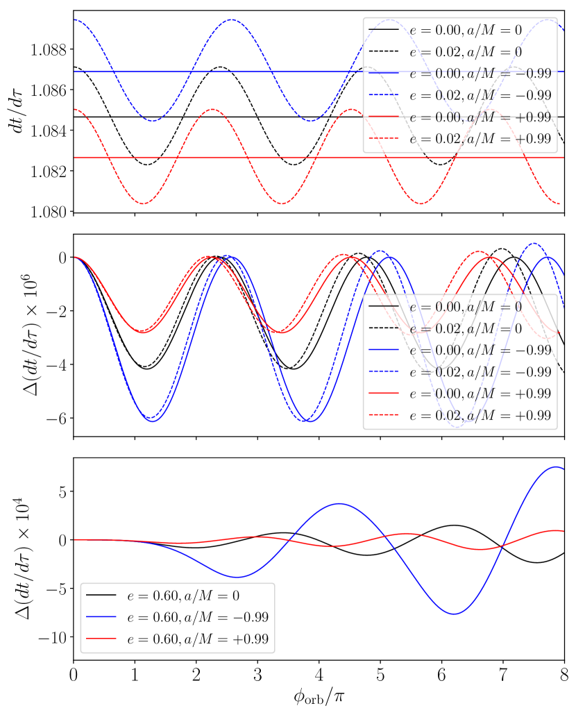
Figure 3: (Figure is updated) The time-like component of msp’s 4-velocity $u^{0}={\rm d}t/{\rm d}\tau$ of 4-velocity of the msp, and the corrections due to msp’s spin-orbit and spin-curvature coupling. Upper panel shows the geodesics ${\rm d}t/{\rm d}\tau$ of circular and quasi-circular orbit. Middle panel is the corrections due to spin-orbit and spin-curvature coupling for circular and quasi-circular orbits. Lower panel demonstrate the corrections in ${\rm d}t/{\rm d}\tau$ due to spin-orbit coupling for elliptical orbits. Note that, the scale of $y$-axis are different for all three panels. The initial spin is $\theta_{\rm spin}=\pi/4$, leaning in the direction towards black hole. All other parameters are the same as in Fig. 2.

When the axis of the spin is not aligned with the angular momentum, the spinning axis, as well as the orbital angular momentum undergoes precession. This effect was investigated previously, either based on a one-graviton interaction analog (e.g. Barker et al., 1966; Barker & O’Connell, 1979), or by approaches similar to this work (e.g. Bini et al., 2005). As the orbital angular momentum, as well as the spin, precesses around the total angular momentum, when such in-plane spin is present, the orbital angular momentum is no longer constant, in either magnitude or direction. The precession of the orbital plane, as a consequence, is usually referred to as out-of-plane motion (Singh et al., 2014).

The focus of this work is on the spin dynamics, and we will present the numerical results and the observables in the following. Typically, there are three different motions related to the spin: precession, nutation and rotation, corresponding to three Euler angles respectively. The choice of Euler angles is subject to the choice of the observer and reference frame. Here we choose the first Euler angle (which describes the precession) to be $\phi_{\rm spin}$, and the second Euler angle (which describes the nutation) to be $\theta_{\rm spin}$. The third Euler angle would be of interest for modelling the motion of the magnetic field axis with respect to the spin axis. As the time scale of rotation of magnetic field axis is $P_{\rm s}=1~{}{\rm ms}$, which is much smaller than the time scale of precession and nutation, we will not include its effect until Sec. 4.1.

The precession of the spinning axis of msp is shown in the upper panel of Fig. 4. Despite that, in this figure, the mass of the massive black hole is $10^{3}\;\!{\rm M}_{\odot}$, the upper panel is valid for BHs with larger masses. The reason is that, on the Newtonian order the spin $\boldsymbol{s}$ of the msp evolves as

$$\boldsymbol{\dot{s}}=\frac{1}{r^{3}}\left(\frac{3M}{2m}(\boldsymbol{L}\times\boldsymbol{s})-\boldsymbol{S_{\rm MBH}}\times\boldsymbol{s}+3(\boldsymbol{\hat{n}}\cdot\boldsymbol{S_{\rm MBH}})(\boldsymbol{\hat{n}}\times\boldsymbol{s})\right)$$ (19)

(see Barker & O’Connell, 1979; Thorne & Hartle, 1985; Kidder, 1995), where $\boldsymbol{L}$ is the orbital angular momentum, the leading order of which is the Newtonian orbital angular momentum $\boldsymbol{L_{\rm N}}=m\boldsymbol{r}\times\boldsymbol{v}$. The precession frequency due to the Newtonian angular momentum is

$$\omega_{L_{\rm N}}=\frac{1}{r^{3}}\frac{3M}{2m}\;\!\left|\boldsymbol{L_{\rm N}}\right|\propto\frac{M}{r^{2}}v\ .$$ (20)

The orbital frequency is however $\omega_{\rm orb}\propto{v}/{r}$, which differs from the above precession frequency by a factor of ${M}/{r}$. Therefore, the ratios of spin’s precession velocities and orbital velocities remain the same for different black hole masses $M$ with the same $r/M$. As shown in the upper panel of Fig. 4, the precession rates descend, $\propto{M}/{r}$, with increasing radius $r$ for all the cases.

The differences in the precession velocity for the spinning black holes with respect to that of the Schwarzschild black hole, as shown in the upper panel of Fig. 4 are due to the second term of Eq. 19. The precession frequency caused by $\boldsymbol{S}_{\rm MBH}$ is

$$\omega_{S_{\rm MBH}}=\frac{1}{r^{3}}\left|\boldsymbol{S_{\rm MBH}}\right|\propto\frac{a}{M}\frac{M^{2}}{r^{3}}\propto\frac{a}{M}\sqrt{\frac{M}{r}}\omega_{L_{\rm N}}\ .$$ (21)

The relation is consistent with that resulted from the mpd equation, which is shown in the upper panel of Fig. 4, despite that the derivations of the two are not based on identical assumptions.

The lower panels of Fig. 4 demonstrate the combined effect of the spin-orbit and spin-spin couplings on the spin precession rate of the msp. The effect is non-linear and is not easily seen from the Eq. 19. However, we can estimate the order of magnitude of it on the spin precession rate in terms of an effective spin (Eq. 18), which may be expressed as

$$\omega_{s}\sim\frac{1}{r^{3}}\frac{M}{m}\left|\boldsymbol{s}\right|\propto\frac{s}{m^{2}}\frac{m}{M}\frac{M^{2}}{r^{3}}\propto\frac{s}{m^{2}}\frac{m}{M}\omega_{L_{\rm N}}\ .$$ (22)

As there is an ${m}/{M}$ dependence, this spin coupling cannot be ignored especially for systems that are consist of intermediate-mass-ratio binaries.

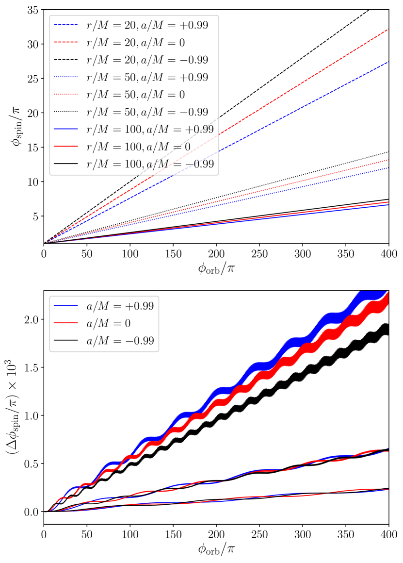
Figure 4: The upper panel shows the precession in $\phi_{\rm spin}$ for circular and quasi-circular geodetic orbits. The semi-major axis of the orbit of the msp is $r=20\;\!M$ (dashed lines), $r=50\;\!M$ (dotted line) and $r=100\;\!M$ (solid line). The black, red, blue lines correspond to the black hole spin $a/M=-0.99$ (i.e. retrograde msp orbit), $0$, and $0.99$ (i.e. prograde msp orbit). The eccentricity of the msp orbit is approximately $0$, and the central black hole is of mass $10^{3}\;\!M_{\odot}$. The initial spin of the neutron star is inclined at an angle $\theta_{\rm spin}=\pi/4$, and leaning in the direction toward the black hole (i.e. $\phi_{\rm spin}=\pi$). The other parameters are the same as those in Fig. 2, The lower panel shows the correction for the precession $\phi_{\rm spin}$ in the presence of spin-orbit coupling, and the orbital parameters are the same as the corresponding ones in the upper panels.

The nutation of the msp’s spinning axis is caused by the combination of the geodesics effect (which only involve the space-time around the black hole), and the coupling of msp’s spin to the orbital angular momentum and to the MBH’s spin. The nutation due to the geodesic effect and the corrections due to msp’s spin are shown in Fig. 5. For Schwarzschild black holes (upper panel, Fig. 5), the total angular momentum

$$\boldsymbol{J}=\boldsymbol{L}+\boldsymbol{s}=\boldsymbol{L}_{\rm N}+\boldsymbol{L}_{\rm PN}+\boldsymbol{L}_{\rm SO}+\boldsymbol{L}_{\rm 2PN}+\boldsymbol{s}\$$ (23)

(Kidder, 1995) is conserved at $2$PN order. When the angular momentum $\boldsymbol{L}_{\rm N}$ wobbles, the orbital plane of the msp will tilt accordingly, and the msp spin axis will also wobbles around, changing the direction and magnitude of the spin 3-vector ${\boldsymbol{s}}$ of the msp.

The msp orbital angular momentum is an external angular momentum. It is conserved when there is a rotational symmetry. This symmetry is however broken in the presence of the msp spin. The situation is slightly different for the msp spin, as it is an intrinsic feature of the msp.

The change of the magnitude of msp spin’s 3-vector is a unique phenomenon, revealed in the mpd equations, whilst it would remain constant in the usual PN formulations (Barker & O’Connell, 1979; Thorne & Hartle, 1985; Kidder, 1995). Although these two descriptions of the evolution of spin seem to be contradictory, they are, in fact, consistent with each other. In the PN formulations, the evolution equation of a particle’s spin is usually written as an outer product of a external angular momentum vector with the particle’s spin vector (e.g. Eq. 19), which directly implies the conservation of the spin’s magnitude. This, however, is written in the comoving frame of the particle, and it has been shown to be equivalent to Fermi-Walker transport equation (see Pastor Lambare, 2017). By contrast, the mpd formulation is written in the distant observer’s frame . It seems that the different choices of reference frame can account for the difference between mpd formulation and PN formulations. But there are still ambiguity in the definition of spin 4-vector, and the physical meaning of the time component $s^{0}$ is not well understood. By using the analogy between spin and relativistic angular momentum, it can be shown that $s^{0}$ is related to the dynamic mass moment , i.e. the offset of centre of mass and centre of momentum, measured by the comoving observer.

Recall the closure condition Eq. 14, which can also be written as $p^{\alpha}s_{\alpha}=0$ (Costa & Natário, 2014) and hence

$$u^{\alpha}s_{\alpha}=0\ .$$ (24)

Dividing both sides by $u^{0}$, the 4-velocity is converted into velocity with respect to the coordinate time:

$$s_{0}=-\left(s_{1}\frac{{\rm d}r}{{\rm d}t}+s_{2}\frac{{\rm d}\theta}{{\rm d}t}+s_{3}\frac{{\rm d}\phi}{{\rm d}t}\right)\ ,$$ (25)

where $s_{\mu}$ are the components of dual vector, defined as $s_{\mu}=g_{\mu\nu}s^{\nu}$. Eq. 25 describes the projection of spin 3-vector onto the velocity measured by a local static observer. Besides, the factor $u^{0}$ describes the time dilation effect, therefore, $s_{0}$ is also related to the relativistic light aberration as described in Rafikov & Lai (2006).

Fig. 5 and Fig. 6 show the nutation of spin axis of the msp due to the spin-orbit coupling. In Fig. 5, we selected the special cases $\theta_{\rm spin}=\pi/2$, where msp’s spin is within the orbital plane, for an example. When $\lambda=0$, the spin rotates around the orbital angular momentum and the spinning angular momentum of the MBH, therefore, there is only change in the first Euler angle $\phi_{\rm spin}$. This explains why in all three panels, when $\lambda=0$, there is no nutation. Nevertheless, when we include spin-orbit coupling, a small nutation occurs. Such an nutation cannot be explained by Eq. 19, nor the first order correction to it by replacing $\boldsymbol{L}$ wth $\boldsymbol{L_{\rm N}}+\boldsymbol{L_{\rm PN}}$, as both of them would lead to vanishing projection of $\dot{{\boldsymbol{s}}}$ onto the $\boldsymbol{L_{\rm N}}$ direction. Thus we need higher order corrections, which, naturally, explains why the order of nutation due to the spin-orbit coupling is smaller than the precession due to spin-orbit coupling by an order.

In fact, most of the orbital components of total angular momentum in Eq. 23 are parallel to $\boldsymbol{L_{\rm N}}$, and the only one that could account for such nutation is $\boldsymbol{L_{\rm SO}}$. From Kidder (1995), we have

$$\boldsymbol{L_{\rm SO}}= \frac{m}{M}\bigg{\{}\frac{M}{r}\boldsymbol{\hat{n}}\times\bigg{[}\boldsymbol{\hat{n}}\times\left(3(\boldsymbol{s}+\boldsymbol{S}_{\rm MBH})+(m-M)\left(\frac{\boldsymbol{S_{\rm MBH}}}{M}-\frac{\boldsymbol{s}}{m}\right)\right)\bigg{]}$$ (26)

$$-\frac{1}{2}\boldsymbol{v}\times\bigg{[}\boldsymbol{v}\times\left(\boldsymbol{s}+\boldsymbol{S_{\rm MBH}}+(m-M)\left(\frac{\boldsymbol{S_{\rm MBH}}}{M}-\frac{\boldsymbol{s}}{m}\right)\right)\bigg{]}\bigg{\}}\ .$$

The scale of it is:

$$\left|\boldsymbol{L_{\rm SO}}\right|\propto \frac{s}{m^{2}}\frac{m^{2}M}{r}\simeq\frac{s}{m^{2}}\frac{m}{M}\sqrt{\left(\frac{M}{r}\right)^{3}}\ \left|\boldsymbol{L_{\rm N}}\right|\ .$$ (27)

Therefore the frequency of nutation due to $\boldsymbol{L_{\rm SO}}$ is

$$\omega_{L_{\rm SO}}=\frac{1}{r^{3}}\frac{3M}{2m}|\boldsymbol{L_{\rm SO}}|\propto\frac{s}{m^{2}}\frac{m}{M}\frac{M^{3}}{r^{4}}\propto\frac{s}{m^{2}}\frac{m}{M}\sqrt{\left(\frac{M}{r}\right)^{3}}\ \omega_{L_{\rm N}}\ .$$ (28)

In Eq. 26, when we set $\boldsymbol{S_{\rm MBH}}$ to be zero, the only part that contributes to the nutation is

$$\boldsymbol{L}_{\rm SO}\simeq \frac{m}{M}\bigg{\{}\frac{M}{r}\frac{M}{m}\boldsymbol{\hat{n}}\times\left[\boldsymbol{\hat{n}}\times\boldsymbol{s}\right]-\frac{1}{2}\frac{M}{m}\boldsymbol{v}\times\left[\boldsymbol{v}\times\boldsymbol{s}\right]\bigg{\}}\ ,$$ (29)

$$\simeq \frac{M}{r}\bigg{\{}\boldsymbol{\hat{n}}\left[\boldsymbol{\hat{n}}\cdot\boldsymbol{s}\right]-\frac{1}{2}\boldsymbol{\hat{v}}\left[\boldsymbol{\hat{v}}\cdot\boldsymbol{s}\right]\bigg{\}}+\text{terms that are parallel to }\boldsymbol{s}\ .$$

The time dependencies of $\boldsymbol{\hat{n}}(\boldsymbol{\hat{n}}\cdot\boldsymbol{s})$ and $\boldsymbol{\hat{v}}(\boldsymbol{\hat{v}}\cdot\boldsymbol{s})$ are the same for circular orbits. Take $\boldsymbol{\hat{n}}(\boldsymbol{\hat{n}}\cdot\boldsymbol{s})$ for an example. Assuming the orbital angular frequency to be $\omega$, the angular frequency of the spin’s precession to be $\Omega$, we have $\Omega\ll\omega$. The value of $\boldsymbol{\hat{n}}(\boldsymbol{\hat{n}}\cdot\boldsymbol{s})$ averaged over an orbital period is

$$\langle\boldsymbol{\hat{n}}(\boldsymbol{\hat{n}}\cdot\boldsymbol{\hat{s}})\boldsymbol{\hat{x}}\rangle= \int\frac{{\rm d}t}{T}\cos(t\omega)\big{[}\sin(t\omega)\sin(t\Omega)+\cos(t\omega)\cos(t\Omega)\big{]}$$ (30)

$$\sim \frac{\sin(t(2\omega-\Omega))}{2(2\omega-\Omega)}+\frac{\sin(t\Omega)}{2\Omega}+\text{constants}\ .$$

The nutation therefore has two frequencies, with the dominate one having the same frequency as the precession of the spin axis (as shown in the upper panel of Fig. 5). The other frequency is not apparent in the Fig. 5, as the precession velocity $\Omega$ varies with frequency $2(\omega-\Omega)$, which cancels out the first term of Eq. 30.

We have not considered the black hole spin explicitly in the above discussion. When we include the MBH’s spin, the situation is much more complicated. Here we present only the numerical results for the case with an initial spin orientation $\theta_{\rm spin}=\pi/2$, in Fig. 5. There are also small amplitude nutation resulting from spin-spin corrections, besides the corrections to the period of spin’s nutation with respect to spin’s precession, and they are shown in the small figures in the right side of each panel.

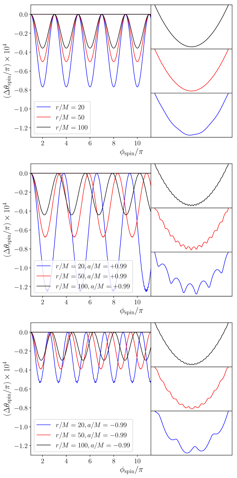
Figure 5: The nutation of $\theta_{\rm spin}$ for the cases with $a/M=0$ (upper panel), $0.99$ (left side, middle panel) and $-0.99$ (lower panel), corresponding respectively to the red, blue and black curves in Fig. 4 respectively. The small amplitude nutations contributed by the spin-spin interaction are shown correspondingly on the right side of each panel. In this figure, the cases with $r=20\;\!M$, $r=50\;\!M$ and $r=100\;\!M$ are respresnted by blue, red and blue respectively. The initial spin of the msp is inclined at an angle $\theta_{\rm spin}=\pi/2$ and leaning in the direction toward the black hole (i.e. $\phi_{\rm spin}=\pi$). The other parameters are the same as those in Fig. 4. The horizontal straight line at $\theta_{\rm spin}=0$ in each panel is the reference of no nutation, the geodesic case.

The nutation due to spin-orbit coupling for a general case, with $\theta_{\rm spin}=\pi/4$, is shown in Fig. 6. It demonstrates that the spinning axis of the msp undergoes nutation even without spin-orbit coupling. This nutation comes from Thomas precession (or equivalently Eq.19 in the distant observer’s frame). As shown in Fig. 6 (upper panel), the geodesic nutation is affected by the alignment of the msp’s velocity and its spinning axis in the distant observer’s frame, and it has a angular frequency roughly of $2(\omega-\Omega)$. The amplitude is approximated by a Lorentz transformation from the comoving frame to the local static frame, and has value

$$\Delta\theta_{\rm spin}\simeq\tan^{-1}\left(\frac{2(\gamma-1)\sin^{2}\left(\theta_{\rm spin}\right)}{(\gamma-1)\sin\left(2\theta_{\rm spin}\right)+2}\right)\ ,$$ (31)

where $\gamma=(1-{M}/{r})^{-1/2}$ is the Lorentz factor, $\theta_{\rm spin}$ is the initial angle of spin. As shown in the upper panel of Fig. 6, for $\theta_{\rm spin}=\pi/4$ and $r/M=20$, $\Delta\theta_{\rm spin}\simeq 0.004\;\!\pi$, a value that is consistent with that obtained by solving the mpd equation directly. When the spin-couplings are included in the mpd equation (i.e. $\lambda=1$ in Eq. 15,16,17), the corrections have two frequencies. The lower frequency is similar to the one shown in Fig. 5 and Eq. 30, while the higher frequency is due to the shift of the precession velocity, and therefore roughly has a frequency of $2\;\!(\omega-\Omega)$. The modulations of the $\Delta\theta_{\rm spin}$ amplitude shown in the lower two panels of Fig. 6 are the consequences of the variations of $\gamma$ over the orbital cycle.

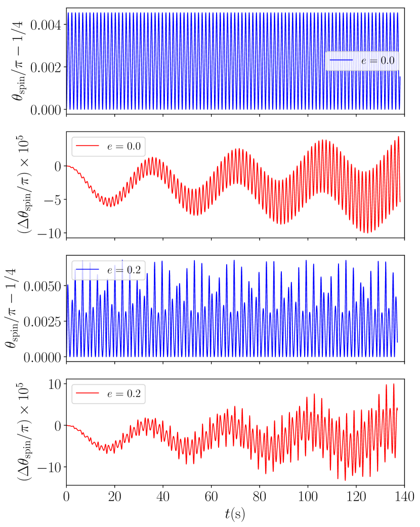
Figure 6: Nutation of spin axis due to geodesics (blues lines, 1st and 3rd panels from above), and the corrections to nutation due to the coupling of msp’s spin. In the upper two panels, the eccentricity of the msp’s orbit is $e=0$, in the lower two panels, $e=0.2$. The MBH’s spin is $a/M=0$, and the semi-major axis of the orbit of msp are $r=20\;\!M$. Other parameters are the same as those used in Fig. 4

4 Discussion

4.1 Observational prospects

The results presented have several observational prospects. The waveform of gravitational wave emitted by a eccentric binary system has been a heated topic in both equal and extreme mass ratio systems (Favata, 2014; Kavanagh et al., 2017; Moore et al., 2018). emri / imri are expected to possess large orbital eccentricities when they enter the lisa frequency band (see Amaro-Seoane et al., 2007; Amaro-Seoane, 2018). Ignoring the orbital eccentricity may lead to systematic biases in parameter estimation of compact binary gravitational wave sources (Favata, 2014) and also to loss in the source detection (Moore et al., 2018). lisa is expected to be more sensitive to the orbital eccentricity of the binary systems than ligo, and the problem would therefore be severe. Despite the technical difficulties, modelling the waveforms of the eccentric binary systems is essential, as emri / imri with high eccentricity are favourable target systems of lisa – the high eccentricity leads to stronger signal and hence an enhancement of detectable events (Barack & Cutler, 2004; Amaro-Seoane et al., 2015). Constructing waveform templates with high accuracy is therefore a very crucial objective in the preparation of future lisa observations, as well as in full exploitation of the ligo capability.

In this calculation, energy dissipation is not considered, and hence its effect on the eccentricity evolution is not included. The time scale of eccentricity evolution is however comparable to the time scale of orbital decay (see Peters, 1964). It therefore justifies our approximation that the eccentricity does not vary on the time scale of spin precession and nutation. Note that the spin-orbit coupling will introduce a shift in the phase of the gravitational wave emitted, and the accumulative effect of spin on the phase of gravitational wave of the circular system was studied by (Burko & Khanna, 2015; Warburton et al., 2017; Fujita, 2018).

Besides gravitational wave, the spin-orbit coupling effect can be observed in pulsar timing observation. The correction to orbital precession would introduce extra shift of pulses received by a distant observer, and the spin precession and nutation could lead to the variation of pulse profiles, the detection of which has been shown to be possible (Kerr, 2015). To estimate the effect of spin’s precession and nutation, we adopt a toy model, using the light house model of pulsar here, as shown in Fig. 7. In Fig. 7, we do not use the Euler angles defined above. Instead, we fix the spin vector, while moving the observer relative to the centre of msp, in a way that could mimic both precession and nutation. The spin axis $\boldsymbol{\hat{S}}$ is fixed in the $x-z$ plane, such that the magnetic field line $\boldsymbol{\hat{M}}$ is initially aligned with the $x$-axis, and rotate around the spin axis with period $P_{\rm s}=1\;\!{\rm ms}$. The angle between $\boldsymbol{\hat{M}}$ and $\boldsymbol{\hat{S}}$ is $\chi$. When the spin axis precesses around the angular momentum $\boldsymbol{\hat{L}}=-\boldsymbol{\hat{z}^{\prime}}$, we move the observer on the $x^{\prime}-y^{\prime}$ plane (around $z^{\prime}$) to mimic the precession. When the spin axis nutates slightly in $-\boldsymbol{\hat{L}}=\boldsymbol{\hat{z}^{\prime}}$ direction, we move the observer in $-z^{\prime}$ direction to mimic nutation. Here the $x^{\prime}-y^{\prime}$ plane is inclined at an angle $\iota$ with respect to the original $x-y$. All the vectors used here, including $\boldsymbol{\hat{S}}$, $\boldsymbol{\hat{M}}$ and $\boldsymbol{\hat{O}}$ are unit vectors.

In order to simplify our model, we use a non-rotating massive black hole in the following discussion. Suppose that the precession has an angular frequency $\Omega$, from the results in Eq. 30, the dominate angular frequency of nutation is also $2(\omega-\Omega)$, and the dominate correction to nutation is of frequency $\Omega$, as shown in Fig. 5 and Fig. 6. We write the nutation as $\nu(\Omega,t,\omega)$. The location of the observer at time $t$ is

$$x_{\rm OB}= \cos(t\Omega)\cos(\nu(\Omega,t,\omega))\ ;$$ (32)

$$y_{\rm OB}= \sin(\Omega t)\cos(\nu(\Omega,t,\omega))\cos\iota+\sin(\nu(\Omega,t,\omega))\sin\iota\ ;$$

$$z_{\rm OB}= \sin(\Omega t)\cos(\nu(\Omega,t,\omega))\sin\iota-\sin(\nu(\Omega,t,\omega))\cos\iota\ .$$

As the time scale of the precession is much larger than the rotation time scale, we can first ignore the rotation, and assume that whenever the unit vector of the observer (i.e. the line-of-sight) is inside the rings wrapping the magnetic field axis, the observer would receive pulses, with width equivalent to the arc length. The emission cone is assumed to have an half open angle $\theta_{\rm cone}$. The width of the pulse is therefore:

$$w= 2\sin\theta_{\rm cone}\sqrt{1-\frac{\tan^{2}\theta_{MO}}{\tan^{2}\theta_{\rm cone}}}\text{ when $\theta_{MO}\leq\theta_{\rm cone}$}\ ,$$ (33)

where $\theta_{MO}$ is the angle between unit vectors $\boldsymbol{\hat{O}}$ and $\boldsymbol{\hat{M}}$, where $\boldsymbol{\hat{M}}$ is rotated such that it’s in the same plane as $\boldsymbol{\hat{S}}$ and $\boldsymbol{\hat{O}}$. The angle $\theta_{MO}$ can therefore be determined by

$$\theta_{MO}=|\cos^{-1}(\boldsymbol{\hat{S}}\cdot\boldsymbol{\hat{O}})-\chi|\ .$$ (34)

When we include the the rotation of the msp, as shown by the upper panel of Fig. 7, as the observer moves from $\boldsymbol{\hat{O}}$ to $\boldsymbol{\hat{O}^{\prime}}$, the emission it receives is triggered by magnetic field $\boldsymbol{\hat{M}^{\prime}}$. Therefore, there is a shift of emission time, either delayed or advanced by

$$\Delta t =\frac{1}{\pi}\left|\;\sin^{-1}\left(\frac{\sin(\theta_{MM^{\prime}}/2)}{\sin\chi}\right)\;\right|P_{\rm s}\ ,$$ (35)

where $\theta_{MM^{\prime}}$ is the angle between $\boldsymbol{\hat{M}}$ and $\boldsymbol{\hat{M}^{\prime}}$. The angle $\theta_{MM^{\prime}}$ can be calculated by using

$$\sin\left(\frac{\theta_{MM^{\prime}}}{2}\right) =\sqrt{\frac{1-\cos\theta_{MM^{\prime}}}{2}}=\sqrt{\frac{1-\boldsymbol{\hat{M}}\cdot\boldsymbol{\hat{M}^{\prime}}}{2}}\ ;$$ (36)

$$\boldsymbol{\hat{M}^{\prime}} =\frac{\sin(\theta_{w}+\chi)}{\sin\theta_{w}}\boldsymbol{\hat{S}}+\frac{\sin\chi}{\sin\theta_{SO}}(\boldsymbol{\hat{O}}-\boldsymbol{\hat{S}})\ ,$$

where $\theta_{w}=\left(\pi-\theta_{SO}\right)/2$, and $\theta_{SO}=\cos^{-1}(\boldsymbol{\hat{S}}\cdot\boldsymbol{\hat{O}})$.

Take $\theta_{\rm cone}=10^{\circ}$, and $\chi=45^{\circ}$ for an example. We used the data $(r=20M,a=0)$ from Fig. 6. We consider only the leading order precession and nutation due to geodesics, and the leading order correction due to the coupling of the msp’s spin. We write the nutation as

$$\nu(\Omega,t,\omega)=\theta_{\rm geo}\left[1-\cos 2(\omega-\Omega)t\right]+\theta_{\rm cor}\left[\cos(\Omega t)-1\right]\ ,$$ (37)

where $\theta_{\rm geo}$ is the scale of nutation for geodesics motion, $\theta_{\rm cor}$ is the scale of nutation, and both are positive number. The values of $\omega,\Omega,\theta_{\rm geo}$ and $\theta_{\rm cor}$ for geodesics motion and the leading order corrections are given in Table. 2. The variation in pulse width, and time shift are shown in Fig. 8.

	geodesics		corrections
$\omega$	$2.2739~{}{\rm rad}/{\rm sec}$	$\delta\omega$	$-7.4411\times 10^{-5}~{}{\rm rad}/{\rm sec}$
$\Omega$	$0.17747~{}{\rm rad}/{\rm sec}$	$\delta\Omega$	$1.2599\times 10^{-5}~{}{\rm rad}/{\rm sec}$
$\theta_{\rm geo}$	$7.1780\times 10^{-3}~{}{\rm rad}$	$\delta\theta_{\rm geo}$	$0$
$\theta_{\rm cor}$	$0$	$\delta\theta_{\rm cor}$	$8.5512\times 10^{-5}~{}{\rm rad}$

Table 2: The values of recession speed and nutation scale for data $(r=20M,a=0,\theta_{\rm spin}=\pi/4,\phi_{\rm spin}=\pi)$ in Fig. 6. Only leading order precession and nutation are considered in order to demonstrate the effect of msp’s spin on the width and time shift of pulses. The corresponding results are shown in Fig. 8.

Besides changing the width and time shift of the pulse, the coupling of spin also results in the shift of pulse disappearing and appearing times, i.e. the times when $w=0$ in the upper panel of Fig. 8. The disappearing and appearing time, denoted by $t_{i}$ are the $i$th solutions to $\tan^{2}\theta_{MO}=\tan^{2}\theta_{\rm cone}$, which is equivalent to:

$$f(t,\Omega,\omega,\theta_{\rm geo},\theta_{\rm cor})\equiv\boldsymbol{\hat{S}}\cdot\boldsymbol{\hat{O}}=\cos(\chi\pm\theta_{\rm cone})\ ,$$ (38)

where we adopt the geodesics values of $(\Omega,\omega,\theta_{\rm geo},\theta_{\rm cor})$ as in Table. 2. The variations of $t_{i}$ can be found by solving the equation Eq. 38 with $\omega\rightarrow\omega+\delta\omega$, $\Omega\rightarrow\Omega+\delta\Omega$, $\theta_{\rm geo}\rightarrow\theta_{\rm geo}+\delta\theta_{\rm geo}$ and $\theta_{\rm cor}\rightarrow\theta_{\rm cor}+\delta\theta_{\rm cor}$. The variations $\delta t_{i}$ are shown in Table. 3. Such a shift is possible to be detected with the instrumental precision of pulsar timing that we can achieve in the near future.

The time shift in Table. 3 is valid for MBH between $10^{3}-10^{6}{\rm M}_{\odot}$, and accumulates with about $\sim-2.5\mu{\rm s}$ every spin’s precession period $T={2\pi}/{\Omega}$, regardless of the mass of massive black hole.

$\iota$	$\delta t_{1}({\rm ns})$	$\delta t_{2}({\rm ns})$	$\delta t_{3}({\rm ns})$	$\delta t_{4}({\rm ns})$
0	-38.72			-3613.66
15	-32.88			-2887.72
30	-141.64			-2113.76
45	-185.35	23.34	-224.91	-1987.59
60	-77.88	-242.83	-368.60	-2246.72
75	-70.66	-391.80	-539.21	-2397.76
89	-69.65	-541.13	-685.78	-2441.96

Table 3: The variation in the disappearing and appearing time of the pulses. Here $t_{1,2,3,4}$ correspond to the instants, when the pulse signal (1) first leaves the emission cone for the first time, (2) re-enter the emission cone for the first time, (3) re-leave th emission cone for the second time, (4) and re-enter the emission cone for the second time within one precession period (i.e. within $0<\Omega t<2\pi$). Note that for $\iota=0,15,30$, the observer’s line of sight doesn’t re-enter the emission cone until the end of a precession period, therefore, we will skip $t_{2}$, $t_{3}$, and label the first re-entering time as $t_{4}$.

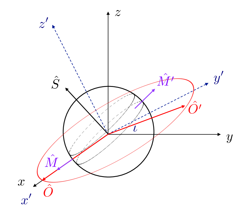
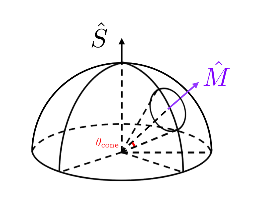
Figure 7: Geometry of the msp’s emission. $\boldsymbol{\hat{S}}$ denotes the spin axis of the msp, $\boldsymbol{\hat{M}}$ is the magnetic axis and is rotating around $\boldsymbol{\hat{S}}$. The circles on the sphere surrounding the magnetic axis denotes the upper and lower boundary of the radiation beam of msp, integrated in time. The precession of the spin axis is achieved by moving the observer $\boldsymbol{\hat{O}}$ on the red circle in the $x^{\prime}-y^{\prime}$ plane, while fixing the direction of the spin’s axis. Note that, the nutation of spin axis is not included and demonstrated in the figure, and can be achieved by perturbing the observer’s circular trajectory in $z^{\prime}$ direction. The observer receives the pulses when the unit vector is in between the two circles of radiation beam, as shown by Eq. 33. The $x^{\prime}-y^{\prime}$ plane is inclined at an angle $\iota$ with respect to the original $x-y$ plane. This angle can be transformed into the inclination angle of the msp orbit using Eq. 32.

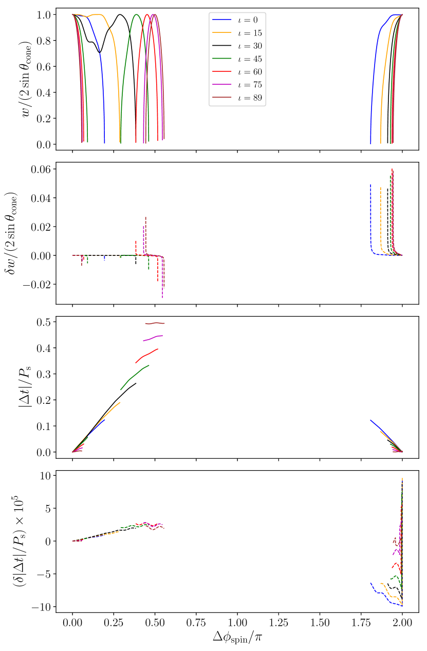
Figure 8: The $1$st and $3$rd panels show the relative width of each pulse $w$ (compared with the maximum possible width $2\sin\theta_{\rm cone}$) and the shift of emission time $\Delta t$ (compared with msp’s intrinsic spinning period $P_{\rm s}$ ) received by a distant observer moving inside $x^{\prime}-y^{\prime}$ plane. The plane is inclined at different angle $\iota$ with respect to the $x-y$ plane. $\iota=90^{\circ}$ was replaced by $89^{\circ}$ to avoid the coordinate singularity. Only geodesics precession and nutation are included in the The 2nd upper panel is the variation in width when including the effect of msp’s spin, the dashed lines corresponds to the solid lines with the same colour in the 1st panel. The 4th panel is the corresponding corrections to the shift of emission time in 3rd panel due to msp’s spin. The corrections due to msp’s spin is shown in the Table. 3

4.2 Pulsars orbiting around a massive black hole

Large population of pulsars are believed to reside in the central region of our galaxy (Pfahl & Loeb, 2004; Wharton et al., 2012; Zhang et al., 2014), and pulsar population is believed to be dominated by msp, the species that existing pulsar searches are not sensitive to (Macquart & Kanekar, 2015). Several indirect pieces of evidence have been supporting this prediction, for example, excessive gamma-ray emission (Brandt & Kocsis, 2015) (although dark matter could as well account for such gamma-ray detections), the detection of rare magnetar (Rea et al., 2013; Eatough et al., 2013; Mori et al., 2013), and the dense stellar environment in the galactic centre. Very few pulsars have been found until now, and it is believed that the strong scattering of the radio wave by interstellar medium and severe dispersion along the line-of-sight reduce the chance for pulsars to be detected (Cordes & Lazio, 1997; Lazio & Cordes, 1998). Especially, for msp, the temporal smearing at low frequencies is severe (Macquart et al., 2010), and current detectors are not sensitive enough to detect msp as they are of low luminosity at high frequency (Bower et al., 2018). Despite the null detection, prediction of the pulsar population in the central region of our galaxy has been made with different models and assumptions. Constraints from gamma-ray and radio observations predicted $\leq 10^{3}$ msp inside $1\,{\rm pc}$ (Wharton et al., 2012), and up to $10^{4}$ msp inside $1\,{\rm pc}$ (depending on the scattering and absorption, see Rajwade et al., 2017, for details). Simulations by Zhang et al. (2014) predicted $\sim 10$ pulsars inside $\leq 1000\,{\rm au}$, where they assumed that massive stars were captured by central black hole by tidal disruption of stellar binaries. However, these studies on pulsar in the galactic centre are focused on the non-relativistic regime, where the effect of the pulsar’s spin is not important. Indeed, the event rate of discovering a pulsar in the close vicinity of our galactic nuclear black hole is quite low. The complicated environment in the galactic centre makes pulsars difficult to be detected, even if they exist.

Pulsars on orbits with an intermediate-mass black hole (i.e. imrb) are potentially more promising sources. Observations have shown that large galaxies contain a massive nuclear black hole and some may have two, e.g. M83 (Thatte et al., 2000). The masses of these nuclear black holes are found to correlate with the dynamical properties, and hence the mass, of spheroid components of the host galaxies (Magorrian et al., 1998; Ferrarese & Merritt, 2000; Gebhardt et al., 2000). Although the empirical correlations may deviate at the low-mass end where the small galaxies are located (see Graham & Scott, 2015), it does not exclude that ultra-compact dwarf galaxies, globular clusters, or million solar-mass stellar spheroids would contain a black hole at the centre (Perera et al., 2017, see). The masses of the black holes residing in these spheroids are expected to be $\sim 10^{2}-10^{4}~{}{\rm M}_{\odot}$ (Lützgendorf et al., 2013; Mieske et al., 2013), distinguishing them from the stellar-mass black holes in X-ray binaries, e.g. GRO J1655$-$40 (see Soria et al., 1998; Shahbaz et al., 1999) LMC X-3 (see Orosz et al., 2014) in the nearby universe. It is still unclear how and whether a massive nuclear black hole would be formed at the central region of ultra-compact dwarf galaxies or globular clusters. A black hole can grow by accreting gas or capturing stars. In dense stellar environments such as the central region of a ultra-compact dwarf galaxy or the core of a globular cluster, a nuclear black hole, if it is present, could gain mass by coalescing with another black hole, if it is also present, or by capturing stars in its neighbourhood. The recent ligo observations have confirmed that a more massive black hole can be formed by the coalescence of two smaller-mass black holes (e.g. Abbott et al., 2016, 2017b) and a black hole can be produced by merging two neutron stars (Abbott et al., 2017a). Naturally, we can generalise that a more massive black hole can also be formed by merging with a neutron star or a black hole, though such events have not been observed yet. Some studies (e.g. Fragione et al., 2018) indicated that merging of two black holes in a globular cluster would likely cause the remnant system to be ejected. It is, therefore, a concern whether a nuclear black hole would grow to $10^{3}~{}{\rm M}_{\odot}$ through a sequence of black-hole black-hole merging process. Observational studies, however, have shown support for the presence of intermediate-mass black holes (see e.g. Feng & Soria, 2011) in a number of external galaxies. There were also claims (Perera et al., 2017) that intermediate-mass black holes were found in globular clusters. However, these pieces of evidence are not conclusive. Whether or not globular clusters can retain a nuclear intermediate-mass black hole and hence a location of imri would be better resolved by future multimesenger studies, using instruments such as SKA (see Wrobel et al., 2018) and lisa (see e.g. Kimpson et al., 2019a, b).

msp are fast spinning neutron stars on a period of a few to about ten ms (see e.g. Bhattacharya & van den Heuvel, 1991; Papitto et al., 2014) Some newly born neutron stars have a spin period of as short as a few tens of milliseconds, e.g. the Crab pulsar with a spin period of 33 ms (see Manchester et al., 2005). msp are however old neutron stars, found in globular clusters and the galactic bulges. They are believed to have a binary progenitor, and the neutron star was spun up through accreting matter from a companions star (Radhakrishnan & Srinivasan, 1982; Bhattacharya & van den Heuvel, 1991; Ergma & Sarna, 1996; Tauris et al., 2000). Many globular clusters are rich in msp – 25 have been identified in 47 Tucanae (see Manchester et al., 1991; Pan et al., 2016) and 33 in Terzan 5 (see Ransom et al., 2005; Hui et al., 2010). With the abundant msp populations, imrb comprising an msp and a black hole could be formed in the core of a globular cluster (Devecchi et al., 2007; Clausen et al., 2014; Verbunt & Freire, 2014). An estimate of $\sim 1-10$ these msp - black hole binaries in the Galactic globular clusters (see Clausen et al., 2014) would imply that a few tens of such binaries could reside in the globular clusters in the Local Group galaxies, and the pulse emission from the msp could be detected by large ground-base radio telescopes such as the The Square Kilometer Array (SKA) (Keane et al., 2015) and Five hundred meter Apeture Spherical Telescope (FAST) (Nan, 2006).

Although the gravitational radiative loss would have insignificantly effects on the spin and orbital dynamics of the msp in the emrb /imrb considered in this work (see Singh et al., 2014), the power of the gravitational waves emitted from these systems is not negligible. For a system with a black hole with a mass $M=10^{3}\;\!{\rm M}_{\odot}$, a spin parameter $a=0$, and an msp - black hole orbital separation $r=20\;\!M$, the gravitational wave power could reach $\sim 1.6\times 10^{48}\;\!{\rm erg~{}s}^{-1}$ assuming a circular orbit. The corresponding gravitational wave strain $h$ is $3.5\times 10^{-18}$, if the system is located at the core of a globular cluster at a distance of 5 kpc from the Sun, similar to that of 47 Tucanae (Carretta et al., 2000). These systems, which are persistent gravitational wave sources, will eventually evolve to become emri /imrb burst gravitational wave sources, when the msp spirals in and coalesces with the black hole. They are expected to be detectable within the lisa band in the emri /imri stage and also in the emrb /imrb stage.

The significance of these emrb /imrb sources in the context of gravitational wave and multi-messenger astrophysics are of two folds. First of all, the statistics of the emri /imri events arisen from these systems and of the detection of them in the emrb /imrb phase will provide us a mean to determine the abundances of these systems and their populations in various galactic environment. This in turn will constrain their formation channels in dense stellar systems with a resident black hole. Secondly, knowing the population of msp - black holes binaries in globular clusters or other dense stellar spheroids would provide an estimate of the number detectable individual persistent gravitational wave sources, and hence their contribution to the stochastic gravitational wave background. It will serve as a reference when we build models to compute the emri /imri events arisen from neutron star - black hole binaries in the less understood dense stellar environment in the distant Universe.

4.3 Additional remarks

In this work, we assume that the msp is a point pole-dipole, moving in the static Kerr space time. However, in realistic situation, the msp will also curve the space time around it and the background space time will be the consequence of non-linear combination of the msp’s gravity with the black hole’s gravity. The trajectory of the msp will be the geodesics (if we ignore spin-orbit and spin-curvature couplings) of such complicated and evolving space time. Therefore, it’s necessary for us to verify the effect of the msp’s own gravity (so called self-force) on the orbital dynamics and spin dynamics.

The investigation into the effects of the self-force and its comparison with the spin-orbit coupling force has been carried out extensively (e.g. Burko, 2004; Bini & Damour, 2014, 2015; Burko & Khanna, 2015; Barack & Pound, 2018) in different contexts. The magnitude of the first order self-force (in terms of mass ratio $m/M$) is similar to that of the spin-orbit couplings (van de Meent, 2018) (also as shown by comparing results in Barack & Sago, 2011, with Fig. 2). The leading term of the correction to the rate of the spin’s precession due to the conservative part of the first order self-force is (adapted from Eq. (10) or equivalently Eq. (5.4) of Dolan et al., 2014; Bini & Damour, 2014, respectively)

$$\omega_{1{\rm st}}\propto\frac{m}{M}\frac{M}{r}\omega_{L_{\rm N}}\ ,$$ (39)

which is smaller than that due to msp’s spin (i.e. Eq. 22) by a factor of ${M}/{r}$. This self-force correction could be important if we integrate the pulsed signal over a substantial duration.

The leading order of the dissipative self-force is also called radiation-reaction, and it introduces the loss of energy and angular momentum in the emri /imri system (Barack & Pound, 2018). The energy flux and angular momentum flux have been calculated by (Drasco & Hughes, 2006; Fujita et al., 2009; Fujita, 2012; Shah, 2014; van de Meent, 2018) for different orbital configurations. Contribution to the dephasing of gw waveform from dissipative self-force is in general greater than that from conservative self-force and spin-orbit couplings (Burko & Khanna, 2015). To the lowest order, the dissipative self-force can be calculated by solving the energy and angular momentum balance equations (Barack & Sago, 2007; Burko & Khanna, 2013), and we could estimate its effects using the radiative loss formula in Peters (1964) .

From the spin precession angular frequency in Eq. 20, we may define a spin precession period:

$$P_{\rm sp}\approx\frac{2\pi}{\langle\omega_{L_{\rm N}}\rangle}=\frac{4\pi}{3}\frac{r^{5/2}}{M^{2}}\sqrt{m+M}\left(1-e^{2}\right)\ ,$$ (40)

where $\langle\omega_{L_{\rm N}}\rangle$ denotes the average value of $\omega_{L_{\rm N}}$ over an orbital period, under the approximation that the msp follows a Newtonian eccentric orbit. The time-scale for the change in the spin’s precession period due to gravitational radiation is

$$\tau_{\rm gw}\sim\left[\frac{r^{4}}{32mM(m+M)}\right]\,g(e)^{-1}$$ (41)

(see Peters, 1964), where $r$ is the semi-major axis, and $g(e)$ is a function of orbital eccentricity:

$$g(e)=(1-e^{2})^{-7/2}\left(1+\frac{71}{40}e^{2}-\frac{19}{160}e^{4}\right)\ .$$ (42)

Setting $r=\zeta M$, we have

$$\frac{\tau_{\rm gw}}{P_{\rm sp}}\sim\frac{3}{128\pi}\frac{\zeta^{3/2}}{g(e)\left(1-e^{2}\right)}\left(\frac{M}{m}\right)\left(\frac{M}{m+M}\right)^{3/2}\ .$$ (43)

For the systems considered here, $10^{3}{\rm M}_{\odot}\leq M\leq 10^{5}\;\!{\rm M}_{\odot}$ and $20\leq\zeta\leq 100$, implying that ${M}/{m}>6\times 10^{2}$. Moreover, the orbital eccentricity $e\leq 0.4$. This gives $g(e)(1-e^{2})\sim(1-2)$, and ${\tau_{\rm gw}}/{P_{\rm sp}}\sim(2\times 10^{2}-5\times 10^{5})\gg 1$. The application of the mpd formulation is therefore justified.

We would like to emphasize that, the formula above are only valid for orbits with moderate eccentricities. For highly eccentric orbits, ignoring the effects of self-force would lead to substantial errors in modelling the orbital dynamics of the msp. In both cases, including the effects of the self-force will be necessary for modelling secular evolution and the orbital dynamics of msp in an emrb / imrb with high temporal resolutions.

Besides the time shift and width variation of the pulses due to the precession and nutation of the spin, as that shown in Sec. 4.1, and the orbital deviation from geodesic motion (studied in Singh et al., 2014), the bending of light (i.e. gravitational lensing) due to the black hole’s gravity can be non-negligible. To achieve the scientific goals described in this work, we need high temporal and spatial accuracies in the covariant photon transport calculations. A self-consistent calculation as such is computationally challenging and and it also requires advanced numerical techniques, and hence it is beyond the scope of the semi-analytic approached adopted this work. We leave such calculations to future studies.

5 Summary and conclusion

We investigate the spin dynamics of an msp around a massive black hole using the mpd formulation. The extreme mass ratio of the system allows us to consider that the msp is a spinning test mass in a spacetime provided by the black hole. The orbital motion can be described as quasi-geodesics with corrections due to spin-orbit, spin-spin and spin-curvature couplings. These spin couplings lead to precession and nutation of the msp’s spin, besides perturbing the msp’s orbital motion. Such modulations will be detectable in the future gravitational wave experiments, such as lisa, and in pulsar timing observations, with instruments such as SKA and FAST. We have also shown that, the spin-orbit and spin-spin couplings will lead to timing variations between the reference frame of the msp and the observer at a long distance. The timing variation will manifest as variations in the pulsed periods of the pulsar’s emission received by the observer. These results obtained from mpd equations are consistent in order with the weak field approximation.

Appendix A Eccentricity

The eccentricity of the msp’s orbit is set by solving the set of equations:

$$E^{2}{g_{\rm a}}^{00}-2{g_{\rm a}}^{30}EL_{z}+{g_{\rm a}}^{33}L_{z}^{2}= -1$$ (44)

$$E^{2}{g_{\rm b}}^{00}-2{g_{\rm b}}^{30}EL_{z}+{g_{\rm b}}^{33}L_{z}^{2}= -1\ ,$$

with ${g_{\rm a}}^{\mu\nu}$ evaluated at $r_{\rm a}=r(1-e)$ and ${g_{\rm b}}^{\mu\nu}$ at $r_{\rm b}=r(1+e)$, where $r$ is the semi-major axis, and $e$ is the orbit eccentricity.

The expressions for the solutions are complicated. We therefore include only the leading order of $\eta={M}/{r}$ and $e$, so as to demonstrate the leading order effect the of eccentricity and black hole’s spin. We use $\alpha={a}/{M}$, which is a dimensionless factor of the black hole spin. For prograde motion, the two integration constants, $E$ and $L_{z}$, associated with the geodesics are:

$$E =1-\frac{\eta}{2}+\frac{3\eta^{2}}{8}-\alpha\eta^{5/2}+\mathcal{O}\left(\eta^{5/2},e^{2}\right)\ ,$$ (45)

$$L_{z} =\frac{M}{\sqrt{\eta}}+\mathcal{O}\left(\eta^{-1/2},e^{2}\right)\ ,$$

and for retrograde motion,

$$E =1-\frac{\eta}{2}+\frac{3\eta^{2}}{8}+5\alpha\eta^{5/2}+12e\alpha\eta^{5/2}+\mathcal{O}\left(\eta^{5/2},e^{2}\right)\ ,$$ (46)

$$L_{z} =\frac{M}{\sqrt{\eta}}+\mathcal{O}\left(\eta^{-1/2},e^{2}\right)\ .$$

By setting the initial $E$ and $L_{z}$, the eccentricity is accurate for pure geodesic calculations (i.e. setting $\lambda=0$ in Eq. 15,16,17). In such a situation, the 4-momentum and 4-velocity are parallel to each other. For the mpd equation (Eq. 15,16,17 with $\lambda=1$), the eccentricity is slightly different from the expected values by $\delta e\sim 2\times 10^{-5}$, which can be estimated by the comparison of the spin-orbit coupling force with the Newtonian gravitational force:

$$\frac{F_{\rm so}}{F_{\rm New}}\sim\left(\frac{M}{r}\right)^{3/2}\left(\frac{m}{M}\right)\frac{S}{m^{2}}\ .$$ (47)

Appendix B Proper Time

In order to investigate the effect of GR, eccentricity and black hole’s spin on the ratio of the coordinate time over proper time ${{\rm d}t}/{{\rm d}\tau}$, we calculate the approximate $u^{0}$ for quasi-circular orbits, using the $E$ and $L_{z}$ derived in Appendix A.

For prograde motion, the time component of the 4-velocity at $r_{1,2}=r(1\mp e)$ is:

$$u^{0} =-g^{00}E-g^{03}EL_{z}$$ (48)

$$=1+\left(\frac{3}{2}\pm 2e\right)\eta+\left(\frac{27}{8}\pm 7e\right)\eta^{2}-\alpha\eta^{5/2}(3\pm 6e)+\mathcal{O}\left(\eta^{3},e^{2}\right)\ ,$$

where the upper signs denote $r_{1}$, lower signs denote $r_{2}$. For retrograde motion, the $u^{0}$ is equivalent to changing $\alpha$ into $-\alpha$, as we can expected.

This equation doesn’t include the effect of msp’s spin on the orbital $u^{0}$. Such effect can be estimated by means of the formula of spin-orbit coupling force as in Appendix A. As the eccentricity is shifted by $\delta e\sim 2\times 10^{-5}$, the shift of $u^{0}$ is about

$$\Delta u^{0}\sim 2\delta e\eta\ .$$ (49)

References

- Abbott et al. (2016) Abbott B. P., et al., 2016, Phys. Rev. Lett., 116, 061102
- Abbott et al. (2017a) Abbott B. P., et al., 2017a, ApJ, 848, L13
- Abbott et al. (2017b) Abbott B. P., et al., 2017b, ApJ, 851, L35
- Amaro-Seoane (2018) Amaro-Seoane P., 2018, Living Reviews in Relativity, 21, 4
- Amaro-Seoane et al. (2007) Amaro-Seoane P., Gair J. R., Freitag M., Miller M. C., Mandel I., Cutler C. J., Babak S., 2007, Classical and Quantum Gravity, 24, R113
- Amaro-Seoane et al. (2015) Amaro-Seoane P., Gair J. R., Pound A., Hughes S. A., Sopuerta C. F., 2015, in Journal of Physics Conference Series. p. 012002 (arXiv:1410.0958), doi:10.1088/1742-6596/610/1/012002
- Barack & Cutler (2004) Barack L., Cutler C., 2004, Phys. Rev. D, 69, 082005
- Barack & Pound (2018) Barack L., Pound A., 2018, arXiv preprint arXiv:1805.10385
- Barack & Sago (2007) Barack L., Sago N., 2007, Phys. Rev. D, 75, 064021
- Barack & Sago (2011) Barack L., Sago N., 2011, Phys. Rev. D, 83, 084023
- Barker & O’Connell (1979) Barker B. M., O’Connell R. F., 1979, General Relativity and Gravitation, 11, 149
- Barker et al. (1966) Barker B. M., Gupta S. N., Haracz R. D., 1966, Physical Review, 149, 1027
- Beiglböck (1967) Beiglböck W., 1967, Communications in Mathematical Physics, 5, 106
- Bhattacharya & van den Heuvel (1991) Bhattacharya D., van den Heuvel E. P. J., 1991, Phys. Rep., 203, 1
- Bini & Damour (2014) Bini D., Damour T., 2014, Phys. Rev. D, 90, 024039
- Bini & Damour (2015) Bini D., Damour T., 2015, Phys. Rev. D, 91, 064064
- Bini et al. (2005) Bini D., de Felice F., Geralico A., Jantzen R. T., 2005, Classical and Quantum Gravity, 22, 2947
- Bower et al. (2018) Bower G. C., et al., 2018, preprint, p. arXiv:1810.06623 (arXiv:1810.06623)
- Brandt & Kocsis (2015) Brandt T. D., Kocsis B., 2015, ApJ, 812, 15
- Burko (2004) Burko L. M., 2004, Phys. Rev. D, 69, 044011
- Burko & Khanna (2013) Burko L. M., Khanna G., 2013, Phys. Rev. D, 88, 024002
- Burko & Khanna (2015) Burko L. M., Khanna G., 2015, Phys. Rev. D, 91, 104017
- Carretta et al. (2000) Carretta E., Gratton R. G., Clementini G., Fusi Pecci F., 2000, ApJ, 533, 215
- Chicone et al. (2005) Chicone C., Mashhoon B., Punsly B., 2005, Physics Letters A, 343, 1
- Clausen et al. (2014) Clausen D., Sigurdsson S., Chernoff D. F., 2014, MNRAS, 442, 207
- Cordes & Lazio (1997) Cordes J. M., Lazio T. J. W., 1997, ApJ, 475, 557
- Costa & Natário (2014) Costa L. F., Natário J., 2014, preprint, (arXiv:1410.6443)
- Costa et al. (2018) Costa L. F. O., Lukes-Gerakopoulos G., Semerák O., 2018, Phys. Rev. D, 97, 084023
- Damour & Deruelle (1985) Damour T., Deruelle N., 1985, Ann. Inst. Henri Poincaré Phys. Théor., Vol. 43, No. 1, p. 107 - 132, 43, 107
- Damour & Deruelle (1986) Damour T., Deruelle N., 1986, Ann. Inst. Henri Poincaré Phys. Théor., Vol. 44, No. 3, p. 263 - 292, 44, 263
- Damour et al. (2008) Damour T., Jaranowski P., Schäfer G., 2008, Phys. Rev. D, 77, 064032
- Deriglazov & Ramírez (2017) Deriglazov A. A., Ramírez W. G., 2017, International Journal of Modern Physics D, 26, 1750047
- Devecchi et al. (2007) Devecchi B., Colpi M., Mapelli M., Possenti A., 2007, MNRAS, 380, 691
- Dolan et al. (2014) Dolan S. R., Warburton N., Harte A. I., Le Tiec A., Wardell B., Barack L., 2014, Phys. Rev. D, 89, 064011
- Drasco & Hughes (2006) Drasco S., Hughes S. A., 2006, Phys. Rev. D, 73, 024027
- Eatough et al. (2013) Eatough R., et al., 2013, The Astronomer’s Telegram, 5040, 1
- Ergma & Sarna (1996) Ergma E., Sarna M. J., 1996, MNRAS, 280, 1000
- Favata (2014) Favata M., 2014, Phys. Rev. Lett., 112, 101101
- Feng & Soria (2011) Feng H., Soria R., 2011, New Astronomy Reviews, 55, 166
- Ferrarese & Merritt (2000) Ferrarese L., Merritt D., 2000, ApJ, 539, L9
- Fragione et al. (2018) Fragione G., Ginsburg I., Kocsis B., 2018, ApJ, 856, 92
- Frenkel (1926) Frenkel J., 1926, Zeitschrift fur Physik, 37, 243
- Fujita (2012) Fujita R., 2012, Progress of Theoretical Physics, 128, 971
- Fujita (2018) Fujita R., 2018, Gravitational waves from a spinning particle orbiting a Kerr black hole, Gravity and Cosmology, http://www2.yukawa.kyoto-u.ac.jp/~gc2018/slides/1st/Fujita.pdf
- Fujita et al. (2009) Fujita R., Hikida W., Tagoshi H., 2009, Progress of Theoretical Physics, 121, 843
- Gebhardt et al. (2000) Gebhardt K., et al., 2000, ApJ, 539, L13
- Graham & Scott (2015) Graham A. W., Scott N., 2015, ApJ, 798, 54
- Hobbs et al. (2006) Hobbs G. B., Edwards R. T., Manchester R. N., 2006, MNRAS, 369, 655
- Hobbs et al. (2014) Hobbs G., Dai S., Manchester R. N., Shannon R. M., Kerr M., Lee K. J., Xu R., 2014, preprint, p. arXiv:1407.0435 (arXiv:1407.0435)
- Hopman & Alexander (2005) Hopman C., Alexander T., 2005, ApJ, 629, 362
- Hui et al. (2010) Hui C. Y., Cheng K. S., Taam R. E., 2010, ApJ, 714, 1149
- Iorio (2012) Iorio L., 2012, General Relativity and Gravitation, 44, 719
- Kavanagh et al. (2017) Kavanagh C., Bini D., Damour T., Hopper S., Ottewill A. C., Wardell B., 2017, Phys. Rev. D, 96, 064012
- Keane et al. (2015) Keane E., et al., 2015, Advancing Astrophysics with the Square Kilometre Array (AASKA14), p. 40
- Kerr (2015) Kerr M., 2015, MNRAS, 452, 607
- Kidder (1995) Kidder L. E., 1995, Phys. Rev. D, 52, 821
- Kimpson et al. (2019a) Kimpson T., Wu K., Zane S., 2019a, MNRAS (in press)
- Kimpson et al. (2019b) Kimpson T., Wu K., Zane S., 2019b, MNRAS, p. 110
- Konstantinidis et al. (2013) Konstantinidis S., Amaro-Seoane P., Kokkotas K. D., 2013, A&A, 557, A135
- Lazio & Cordes (1998) Lazio T. J. W., Cordes J. M., 1998, ApJ, 505, 715
- Lorimer (2008) Lorimer D. R., 2008, Living Reviews in Relativity, 11
- Lützgendorf et al. (2013) Lützgendorf N., et al., 2013, A&A, 555, A26
- Macquart & Kanekar (2015) Macquart J.-P., Kanekar N., 2015, ApJ, 805, 172
- Macquart et al. (2010) Macquart J. P., Kanekar N., Frail D. A., Ransom S. M., 2010, ApJ, 715, 939
- Magorrian et al. (1998) Magorrian J., et al., 1998, AJ, 115, 2285
- Manchester et al. (1991) Manchester R. N., Lyne A. G., Robinson C., D’Amico N., Bailes M., Lim J., 1991, Nature, 352, 219
- Manchester et al. (2005) Manchester R. N., Hobbs G. B., Teoh A., Hobbs M., 2005, AJ, 129, 1993
- Mashhoon & Singh (2006) Mashhoon B., Singh D., 2006, Phys. Rev. D, 74, 124006
- Mathisson (1937) Mathisson M., 1937, Acta Physica Polonica, 6, 163
- Merritt et al. (2011) Merritt D., Alexander T., Mikkola S., Will C. M., 2011, Phys. Rev. D, 84, 044024
- Mieske et al. (2013) Mieske S., Frank M. J., Baumgardt H., Lützgendorf N., Neumayer N., Hilker M., 2013, A&A, 558, A14
- Miller et al. (2005) Miller M. C., Freitag M., Hamilton D. P., Lauburg V. M., 2005, ApJ, 631, L117
- Moore et al. (2018) Moore B., Robson T., Loutrel N., Yunes N., 2018, preprint, p. arXiv:1807.07163 (arXiv:1807.07163)
- Mori et al. (2013) Mori K., Gotthelf E. V., Barriere N. M., Hailey C. J., Harrison F. A., Kaspi V. M., Tomsick J. A., Zhang S., 2013, The Astronomer’s Telegram, 5020, 1
- Nan (2006) Nan R., 2006, Science in China: Physics, Mechanics and Astronomy, 49, 129
- Orosz et al. (2014) Orosz J. A., Steiner J. F., McClintock J. E., Buxton M. M., Bailyn C. D., Steeghs D., Guberman A., Torres M. A. P., 2014, ApJ, 794, 154
- Osłowski et al. (2011) Osłowski S., van Straten W., Hobbs G. B., Bailes M., Demorest P., 2011, MNRAS, 418, 1258
- Özel & Freire (2016) Özel F., Freire P., 2016, ARA&A, 54, 401
- Pan et al. (2016) Pan Z., Hobbs G., Li D., Ridolfi A., Wang P., Freire P., 2016, MNRAS, 459, L26
- Papitto et al. (2014) Papitto A., Torres D. F., Rea N., Tauris T. M., 2014, A&A, 566, A64
- Pastor Lambare (2017) Pastor Lambare J., 2017, European Journal of Physics, 38, 045602
- Penrose (2004) Penrose R., 2004, The road to reality : a complete guide to the laws of the universe. London: Jonathan Cape
- Perera et al. (2017) Perera B. B. P., et al., 2017, MNRAS, 468, 2114
- Peters (1964) Peters P. C., 1964, Physical Review, 136, 1224
- Pfahl & Loeb (2004) Pfahl E., Loeb A., 2004, in AAS/High Energy Astrophysics Division #8. p. 15.04
- Plyatsko (1998) Plyatsko R., 1998, Phys. Rev. D, 58, 084031
- Plyatsko & Fenyk (2016) Plyatsko R., Fenyk M., 2016, Phys. Rev. D, 94, 044047
- Plyatsko et al. (2011) Plyatsko R. M., Stefanyshyn O. B., Fenyk M. T., 2011, Classical and Quantum Gravity, 28, 195025
- Quinlan & Shapiro (1989) Quinlan G. D., Shapiro S. L., 1989, ApJ, 343, 725
- Radhakrishnan & Srinivasan (1982) Radhakrishnan V., Srinivasan G., 1982, Current Science, 51, 1096
- Rafikov & Lai (2006) Rafikov R. R., Lai D., 2006, ApJ, 641, 438
- Rajwade et al. (2017) Rajwade K. M., Lorimer D. R., Anderson L. D., 2017, MNRAS, 471, 730
- Ransom et al. (2005) Ransom S. M., Hessels J. W. T., Stairs I. H., Freire P. C. C., Camilo F., Kaspi V. M., Kaplan D. L., 2005, Science, 307, 892
- Rea et al. (2013) Rea N., et al., 2013, ApJ, 775, L34
- Remmen & Wu (2013) Remmen G. N., Wu K., 2013, MNRAS, 430, 1940
- Rosa (2015) Rosa J. G., 2015, Physics Letters B, 749, 226
- Ruangsri et al. (2016) Ruangsri U., Vigeland S. J., Hughes S. A., 2016, Phys. Rev. D, 94, 044008
- Saxton et al. (2016) Saxton C. J., Younsi Z., Wu K., 2016, MNRAS, 461, 4295
- Shah (2014) Shah A. G., 2014, Phys. Rev. D, 90, 044025
- Shahbaz et al. (1999) Shahbaz T., van der Hooft F., Casares J., Charles P. A., van Paradijs J., 1999, MNRAS, 306, 89
- Singh (2005) Singh D., 2005, Phys. Rev. D, 72, 084033
- Singh et al. (2014) Singh D., Wu K., Sarty G. E., 2014, MNRAS, 441, 800
- Soria et al. (1998) Soria R., Wickramasinghe D. T., Hunstead R. W., Wu K., 1998, ApJ, 495, L95
- Stappers et al. (2018) Stappers M. H. T., et al., 2018, Nature, 555, 382
- Tauris et al. (2000) Tauris T. M., van den Heuvel E. P. J., Savonije G. J., 2000, ApJ, 530, L93
- Thatte et al. (2000) Thatte N., Tecza M., Genzel R., 2000, A&A, 364, L47
- Thorne & Hartle (1985) Thorne K. S., Hartle J. B., 1985, Phys. Rev. D, 31, 1815
- Tulczyjew (1959) Tulczyjew W., 1959, Acta Physica Polonica, 18, 393
- Verbunt & Freire (2014) Verbunt F., Freire P. C. C., 2014, A&A, 561, A11
- Warburton et al. (2017) Warburton N., Osburn T., Evans C. R., 2017, Phys. Rev. D, 96, 084057
- Wharton et al. (2012) Wharton R. S., Chatterjee S., Cordes J. M., Deneva J. S., Lazio T. J. W., 2012, ApJ, 753, 108
- Wrobel et al. (2018) Wrobel J. M., Miller-Jones J. C. A., Nyland K. E., Maccarone T. J., 2018, in Kapinska A. D., ed., The 34th Annual New Mexico Symposium, held 9 November 2018 at the National Radio Astronomy Observatory. Edited by A.D. Kapinska. Online at <A href=“http://www.aoc.nrao.edu/events/nmsymposium/2018/program.html”> http://www.aoc.nrao.edu/events/nmsymposium/2018/program.html</A>, p.15. p. 15 (arXiv:1806.06052)
- Zhang et al. (2014) Zhang F., Lu Y., Yu Q., 2014, ApJ, 784, 106
- van de Meent (2018) van de Meent M., 2018, Phys. Rev. D, 97, 104033