Chiral constraints on the isoscalar electromagnetic spectral functions of the nucleon from leading order vector meson couplings

Abstract

Using baryon chiral perturbation theory including vector mesons, we analyse various continuum contributions to the isoscalar electromagnetic spectral functions of the nucleon induced by the leading order couplings.

1 Introduction

A premier tool to analyse the electromagnetic structure of the nucleon are dispersion relations. The physics is encoded in the so-called spectral functions, which feature vector meson resonances and continuum contributions. Much is known about the continuum contribution to the isovector spectral function of the electric and magnetic nucleon form factors, see e.g. Ref. [1] for the most recent and most precise investigation. The situation for the corresponding continuum contributions to the isoscalar spectral functions is different, as discussed in detail in Ref. [2]. Chiral perturbation theory has been used to analyze the three-pion continuum [3, 4] within the threshold region starting at $t_{0}=9M_{\pi}^{2}$. These two-loop contributions, however, turn out to be rather small, because the potential enhancement from the anomalous threshold at $t\simeq 8.9M_{\pi}^{2}$ is efficiently masked by phase space factors. On the other hand, earlier modeling suggests an important contribution from the $\pi\rho$ continuum [5] and dispersion relations have been used to calculate the $K\bar{K}$ contribution [6, 7]. In the sector with strange quarks, there have been suggestions of cancellation between contributios from $K\bar{K}$, $KK^{*}$ and $K^{*}K^{*}$ loops, although these have very different thresholds [8].

In this paper, we want to re-analyze some of these continuum as well as some vector meson contributions to the isoscalar electromagnetic spectral functions based on chiral perturbation theory with explicit vector mesons. This extends the earlier tree-level analyses of vector meson contributions to the nucleon electromagnetic (em) form factors as given e.g. in Refs. [9, 10]. Here, we work at leading one-loop order and consider the vector coupling induced contributions. The paper is organized as follows: In Sec. 2, we briefly recall the pertinent definitions for the electromagnetic form factors and their spectral functions. The $\pi\rho$ contribution is worked out and discussed in Sec. 3. The contributions involving $K$ and $K^{*}$ mesons are given in Sec. 4. We end with a summary and outlook. Some technicalities are given in the Appendix.

2 Isocalar electromagnetic spectral functions

The electromagnetic form factors of the nucleon are defined via the matrix element of the electromagnetic current,

$$\Braket{N(p_{f})}{\bar{q}\gamma^{\mu}Qq}{N(p_{i})}=\;\bar{u}(p_{f})\Big{[}\gamma^{\mu}F_{1}(t)+\frac{i}{2m_{N}}\sigma^{\mu\nu}(p_{f}-p_{i})_{\nu}F_{2}(t)\Big{]}u(p_{i})\leavevmode\nobreak\ ,$$ (1)

with $t=(p_{f}-p_{i})^{2}$ the invariant momentum transfer squared, $m_{N}$ the nucleon mass and $Q$ the quark charge matrix. Throughout, we work in the isospin limit $m_{N}=(m_{p}+m_{n})/2$, with $m_{p}\leavevmode\nobreak\ (m_{n})$ the proton (neutron) mass. The functions $F_{1}(t)$ and $F_{2}(t)$ are the Dirac and Pauli form factors of the nucleon, respectively. In the isospin basis, they can be decomposed into isoscalar and isovector components, following the notation of Ref. [11]

$$F_{i}(t)=F_{i}(t)^{S}+\tau^{3}F_{i}^{V}(t)\leavevmode\nobreak\ ,\quad\quad\quad i=1,2.$$

$F_{1}(t)$ and $F_{2}(t)$ are related to the commonly used electric and magnetic Sachs form factors in the following fashion

$$G_{E}^{S,V}(t)= \;F_{1}^{S,V}(t)+\frac{t}{4m_{N}^{2}}F_{2}^{S,V}(t)\leavevmode\nobreak\ ,$$ (2)

$$G_{M}^{S,V}(t)= \;F_{1}^{S,V}(t)+F_{2}^{S,V}(t)\leavevmode\nobreak\ .$$

An unsubstracted dispersion relation can be written down for each form factor defined by

$$F(t)=\frac{1}{\pi}\int_{t_{0}}^{\infty}\frac{\text{Im}F(t^{\prime})}{t^{\prime}-t-i\epsilon}$$ (3)

where $t_{0}$ is the threshold energy for hadronic intermediate states. Here, we focus entirely on the isoscalar spectral function with $t_{0}=9M_{\pi}^{2}$, as the three-pion state is the lowest mass intermediate state possible. For a more general discussion of the spectral functions, see e.g. Refs. [2, 12, 13].

3 The $\pi\rho$ contribution

In this section we focus on the calculation of the imaginary parts of the isoscalar nucleon electromagnetic form factors generetad from the $\pi\rho$ continuum based on relativistic two-flavor baryon chiral perturbation theory. At lowest order in the quark mass and momentum expansion, the relevant interaction Lagrangians are given by [14, 15, 16]

$$\mathcal{L}_{\pi N}= \;\frac{g_{A}}{2}\bar{\Psi}\gamma^{\mu}\gamma_{5}u_{\mu}\Psi\leavevmode\nobreak\ ,$$ (4)

$$\mathcal{L}_{\rho N}= \;g_{\rho N}\bar{\Psi}\rho_{\mu}\gamma^{\mu}\Psi\leavevmode\nobreak\ ,$$

$$\mathcal{L}_{\omega\rho\pi}= \;\frac{g_{\omega\rho\pi}}{2}\epsilon^{\mu\nu\alpha\beta}\omega_{\nu}\langle\rho_{\alpha\beta}u_{\mu}\rangle\leavevmode\nobreak\ ,$$

$$\mathcal{L}_{\omega\gamma}= \;\frac{f_{\omega}}{2}e(\partial_{\mu}\omega_{\nu}-\partial_{\nu}\omega_{\mu})(\partial^{\mu}\mathcal{A}^{\nu}-\partial^{\nu}\mathcal{A}^{\mu})\leavevmode\nobreak\ .$$

Here, $\Psi$ denotes the nucleon doublet, $\rho_{\mu}$ the isovector-vector $\rho$-meson, $\omega_{\mu}$ the isoscalar-vector $\omega$-meson, ${\cal A}^{\mu}$ the photon field, $\langle\ldots\rangle$ denotes the trace in flavor space and $\epsilon^{\mu\nu\alpha\beta}$ is the totally antisymmetric Levi-Civita tensor with $\epsilon^{0123}=1$. Further, $g_{A}$ is the nucleon axial-vector coupling, $g_{A}\simeq 1.27$, and the various vector meson couplings are taken as $g_{\rho N}=5.92$, $g_{\omega\rho\pi}=11.6$ [17] and $f_{\omega}=0.1$ [18]. In the SU$(2)$ sector, due to the universality of the $\rho$-meson coupling the equality of the $\rho$-meson self-coupling and the coupling to the nucleons $g=g_{\rho N}$, holds [19]. As can be seen from the Lagrangian in Eq. (4), we work in the vector meson dominace approximation, i.e. the photon couples only via vector mesons to the hadrons. This is e.g. realized in the hidden symmetry approach of Ref. [20] for the parameter $a=2$. However, in general, the gauged Wess-Zumino-Witten term also leads to a direct $\gamma\rho\pi$ coupling e.g. in the massive Yang-Mills approach. It can, however, be shown that all these different approaches are equivalent, see e.g. the detailed discussion in Ref. [21]. Our choice is driven by simplicity. For more thorough discussion of the Wess-Zumino-Witten term in the presence of vector mesons and photons, see the reviews [20, 21]. Note also that we neglect the small OZI-violating $\pi$-$\rho$ contribution due to the $\phi$-meson coupling.

The following power counting rules for the loop diagrams are used: vertices from $\mathcal{L}^{(n)}$ count as $\mathcal{O}(q^{n})$, so we count the vector meson, nucleon and pion propagators as $\mathcal{O}(q^{0})$, $\mathcal{O}(q^{-1})$ and $\mathcal{O}(q^{-2})$, in order. Thus the order of the diagrams in Fig. 1 is $\mathcal{O}(q^{7})$ at low energies, i.e. for small $t$.

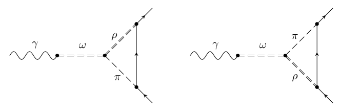
Figure 1: Continuum $\pi\rho$ contribution to the imaginary parts of the isoscalar electromagnetic form factors of the nucleon through the anomalous coupling to the $\omega$. Dashed and solid lines denote pions and nucleons, respectively. The dashed lines represent the $\omega$- and $\rho$-mesons.

We work in the center of momentum frame of the nucleon pair with $q=\big{(}-2E_{p},\leavevmode\nobreak\ \vec{0}\big{)}$. The initial and the final momentum of the nucleons are, respectively, $p_{i}=\big{(}E_{p},\leavevmode\nobreak\ \vec{p}\big{)}$, $p_{f}=\big{(}E_{p},\leavevmode\nobreak\ \vec{p}\big{)}$, with $|\vec{p}|=(t/4-m_{N}^{2})^{1/2}$ and $E_{p}=(m_{N}^{2}+|\vec{p}|^{2})^{1/2}$. To calculate the imaginary part of the amplitude for the diagrams which are shown in Fig. 1, the Cutkosky rules are applied. The imaginary part of the loop diagram corresponds to a cut diagram for the momentum transfer squared $t\geq(M_{\rho}+M_{\pi})^{2}$. For this calculation, we perform a reduction to scalar loop integrals and thus require the basic scalar loop integrals of two- and three- point functions, called $H$ and $F$, respectively,

$$H= \;i\int\frac{d^{4}k}{(2\pi)^{4}}\frac{1}{[k^{2}-{M_{\pi}}^{2}+i\epsilon^{+}][(k+q)^{2}-{M_{\rho}}^{2}+i\epsilon^{+}]},$$ (5)

$$F= \;i\int\frac{d^{4}k}{(2\pi)^{4}}\frac{1}{[k^{2}-{M_{\pi}}^{2}+i\epsilon^{+}][(p_{i}-k)^{2}-{m_{N}}^{2}+i\epsilon^{+}][(k+q)^{2}-{M_{\rho}}^{2}+i\epsilon^{+}]}$$

with $q^{2}=t=(p_{f}-p_{i})$ and $\epsilon^{+}$ stands for $\epsilon\to 0^{+}$. The corresponding imaginary parts can be readily determined

$$\text{Im}\leavevmode\nobreak\ H:\mathcal{H}(t)= \;\frac{M_{\pi}}{8\pi\sqrt{t}}\sqrt{\frac{(M_{\rho}^{2}-M_{\pi}^{2}-t)^{2}}{4M_{\pi}^{2}t}-1}\leavevmode\nobreak\ ,$$ (6)

$$\text{Im}\leavevmode\nobreak\ F:\mathcal{F}(t)= \;\frac{1}{16\pi\sqrt{t}\sqrt{t-4m_{N}^{2}}}\;\log\Bigg{[}\frac{\frac{t-M_{\pi}^{2}-M_{\rho}^{2}}{\sqrt{t-4m_{N}^{2}}}-\sqrt{\frac{M_{\pi}^{4}+(M_{\rho}^{2}-t)^{2}-2M_{\pi}^{2}(M_{\rho}^{2}+t)}{t}}}{\frac{t-M_{\pi}^{2}-M_{\rho}^{2}}{\sqrt{t-4m_{N}^{2}}}+\sqrt{\frac{M_{\pi}^{4}+(M_{\rho}^{2}-t)^{2}-2M_{\pi}^{2}(M_{\rho}^{2}+t)}{t}}}\Bigg{]}\leavevmode\nobreak\ .$$

From these, the expressions for the imaginary part of the isoscalar electric and magnetic form factor can be given as follows

$$\text{Im}\leavevmode\nobreak\ G_{E}^{S}(t) = \frac{3f_{\omega}g_{\omega\rho\pi}g_{\rho N}g_{A}}{2\pi^{2}F_{\pi}^{2}}\frac{t}{(t-m_{\omega}^{2})(t-4m_{N}^{2})}$$ (7)

$$\times \Bigg{[}2(t^{2}m_{N}^{2}+tM_{\pi}^{2}M_{\rho}^{2}-2tM_{\pi}^{2}m_{N}^{2}-2tM_{\rho}^{2}m_{N}^{2}$$

$$+ M_{\pi}^{4}m_{N}^{2}+M_{\rho}^{4}m_{N}^{2}-2M_{\pi}^{2}M_{\rho}^{2}m_{N}^{2})\mathcal{F}(t)+2t(t-M_{\pi}^{2}-M_{\rho}^{2})\mathcal{H}(t)\Bigg{]}\leavevmode\nobreak\ ,$$

$$\text{Im}\leavevmode\nobreak\ G_{M}^{S}(t) = \frac{3f_{\omega}g_{\omega\rho\pi}g_{\rho N}g_{A}}{16\pi^{2}F_{\pi}^{2}}\frac{m_{N}^{2}}{(t-m_{\omega}^{2})(t-4m_{N}^{2})^{2}}$$ (8)

$$\times \Bigg{[}(2tm_{N}^{2}(3M_{\pi}^{4}+3M_{\rho}^{4}-2M_{\pi}^{2}M_{\rho}^{2}+8M_{\pi}^{2}m_{N}^{2}+8M_{\rho}^{2}m_{N}^{2})$$

$$- t^{2}(M_{\pi}^{4}+M_{\rho}^{4}+8m_{N}^{4}-4M_{\pi}^{2}m_{N}^{2}+12M_{\rho}^{2}m_{N}^{2})+2t^{3}(M_{\pi}^{2}+M_{\rho}^{2}+3m_{N}^{2})-t^{4}$$

$$- 8m_{N}^{4}(M_{\pi}^{4}+M_{\rho}^{4}-2M_{\pi}^{2}M_{\rho}^{2}))\mathcal{F}(t)-(t^{2}+tM_{\pi}^{2}+tM_{\rho}^{2})(t+8m_{N}^{2})\mathcal{H}(t)\Bigg{]}\leavevmode\nobreak\ .$$

The resulting electric and magnetic spectral functions ${\rm Im}\leavevmode\nobreak\ G^{S}_{E,M}(t)$ and the weighted spectral functions ${\rm Im}\leavevmode\nobreak\ G^{S}_{E,M}(t)/t^{2}$ are shown in Fig. 2. The magnetic one shows a peak at $t\simeq 1.1\,$GeV², which is consistent with the modelling in Ref. [5], where the calculated $\pi\rho$ distribution was approximated by a sharp vector meson poles with a mass of about 1.1 GeV. For a more detailed comparison, we would also have to include the $\rho$-meson tensor couplings that appear at next-to-leading order.

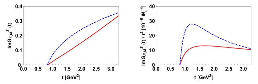
Figure 2: Continuum $\pi\rho$ contribution through the anomalous coupling to the $\omega$ to the isoscalar spectral functions of the electric and magnetic nucleon form factors weighted with and without $1/t^{2}$. The red (solid) and blue (dashed) lines refer to the electric and magnetic form factors, $\text{Im}\leavevmode\nobreak\ G_{E}^{S}(t)$ and $\text{Im}\leavevmode\nobreak\ G_{M}^{S}(t)$, respectively.

4 The contribution from strange loops

Next, we consider the effect of loops with $K\bar{K}$, $KK^{*}$ and $K^{*}K^{*}$ loops. We note, however, that the latter two only start to have an imaginary part at about 2 GeV² and 3 GeV², which is already far inside the resonance dominated region. The relevant effective Lagrangians in the SU(3) basis to obtain the contributions from $K\bar{K}$, $KK^{*}$ and $K^{*}K^{*}$ loops read [20, 21, 22, 23, 24, 25]

$$\mathcal{L}_{V\Phi\Phi}= \;-ig\langle V^{\mu}[\Phi,\partial_{\mu}\Phi]\rangle,$$ (9)

$$\mathcal{L}_{VV\Phi}= \;\frac{1}{\sqrt{2}}G\epsilon^{\mu\nu\alpha\beta}\langle\partial_{\mu}V_{\nu}\partial_{\alpha}V_{\beta}\Phi\rangle,$$

$$\mathcal{L}_{VVV}= \;ig\langle(\partial_{\mu}V_{\nu}-\partial_{\nu}V_{\mu})V^{\mu}V^{\nu}\rangle,$$

$$\mathcal{L}_{BB\Phi}= \;-\frac{F}{2}\langle\bar{B}\gamma^{\mu}\gamma_{5}[u_{\mu},B]\rangle-\frac{D}{2}\langle\bar{B}\gamma^{\mu}\gamma_{5}\{u_{\mu},B\}\rangle,$$

$$\mathcal{L}_{BBV}= \;G_{F}(\langle\bar{B}\gamma^{\mu}[\mathcal{V}_{\mu},B]\rangle+\langle\bar{B}\gamma^{\mu}B\rangle\langle V_{\mu}\rangle)+G_{D}(\langle\bar{B}\gamma^{\mu}\{\mathcal{V}_{\mu},B\}\rangle+\langle\bar{B}\gamma^{\mu}B\rangle\langle V_{\mu}\rangle,$$

$$\mathcal{L}_{\phi\gamma}= \;\frac{e}{3\sqrt{2}}F_{V}(\partial_{\mu}\phi_{\nu}-\partial_{\nu}\phi_{\mu})(\partial^{\mu}\mathcal{A}^{\nu}-\partial^{\nu}\mathcal{A}^{\mu})$$

where $\mathcal{V_{\mu}}$ and $V_{\mu}$ represent the vector meson octet and the vector meson nonet particles, respectively. We take the couplings as $G_{F}=g$ and $G_{D}=0$ which results from the constraint analysis and the perturbative renormalizability condition on the vector meson octet and baryon octet interaction of Ref. [26]. The low-energy constants $D$ and $F$ can be determined by fitting to the semi-leptonic baryon decays at tree level. We use the values $F=0.5$ and $D=0.8$ from Ref. [27]. Throughout, we use the pion decay constant $F_{\pi}$ for the leading order meson decay constant.

In addition to the scalar loop integrals in Eq. (6), we also need the following functions corresponding to the $\bar{K}K$, $K^{*}K^{*}$, $\Lambda\bar{K}K$, $\Sigma\bar{K}K$, $\Lambda K^{*}K^{*}$ and $\Sigma K^{*}K^{*}$ loops with the equal masses

$$P= \;i\int\frac{d^{4}k}{(2\pi)^{4}}\frac{1}{[k^{2}-{M_{i}}^{2}+i\epsilon^{+}][(k+q)^{2}-M_{i}^{2}+i\epsilon^{+}]},$$ (10)

$$J= \;i\int\frac{d^{4}k}{(2\pi)^{4}}\frac{1}{[k^{2}-M_{i}^{2}+i\epsilon^{+}][(k+q)^{2}-M_{i}^{2}+i\epsilon^{+}][(p_{i}-k)^{2}-m_{j}^{2}+i\epsilon^{+}]}.$$

The corresponding imaginary parts are determined as

$$\text{Im}\leavevmode\nobreak\ P:\mathcal{P}_{i}(t)= \;-\frac{1}{16\pi}\sqrt{1-\frac{4M_{i}^{2}}{t}}\leavevmode\nobreak\ ,$$ (11)

$$\text{Im}\leavevmode\nobreak\ J:\mathcal{J}_{j}(t)= \;\frac{1}{16\pi\sqrt{t}\sqrt{t-4m_{j}^{2}}}\;\log\Bigg{[}\frac{M_{i}^{2}-\frac{t}{2}+\frac{1}{2}\sqrt{-4m_{j}^{2}+t}\sqrt{-4M_{i}^{2}+t}}{M_{i}^{2}-\frac{t}{2}-\frac{1}{2}\sqrt{-4m_{j}^{2}+t}\sqrt{-4M_{i}^{2}+t}}\Bigg{]}\leavevmode\nobreak\$$

where $M_{i}$ and $m_{j}$ denote the masses of the $K,K^{*}$ mesons and of the $\Lambda,\Sigma$ baryons, respectively.

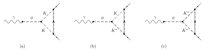
Figure 3: Contributions from $K\bar{K}$, $KK^{*}$ and $K^{*}K^{*}$ loops to the imaginary parts of the isoscalar electromagnetic form factors of the nucleon through the coupling to the $\phi$. The double wiggly, double dashed and dashed lines denote $\phi$-, $K^{*}$- and $K$-mesons, respectively. The dashed solid lines represent either $\Lambda$- or $\Sigma$-baryons. There is an additional permutation of the diagrams in group (b).

We work in the particle basis using the SU(3) symmetric Lagrangian densities given above. An example of such a calculation can be found in the appendix. The imaginary parts of the Sachs form factors for the $KK$ loop are obtained as

$$\text{Im}\leavevmode\nobreak\ G_{E}^{S}(t) = \frac{F_{V}g}{432\sqrt{2}F_{\pi}^{2}{\pi}^{2}m_{N}(t-4m_{N}^{2})(t-M_{\phi}^{2})}$$ (12)

$$\times \Bigg{[}3(D+3F)^{2}t(m_{\Lambda}+m_{N})^{2}(4m_{N}^{5}-4M_{K}^{4}m_{N}-4m_{\Lambda}^{4}m_{N}-2m_{\Lambda}^{2}m_{N}t$$

$$- 2m_{N}^{3}t-m_{\Lambda}^{3}(2t-8m_{N}^{2})-m_{\Lambda}(8m_{N}^{4}-6m_{N}^{2}t+t^{2})$$

$$+ 2M_{K}^{2}(4m_{\Lambda}^{2}m_{N}+m_{N}t+m_{\Lambda}(t-4m_{N}^{2})))\mathcal{J}_{\Lambda}(t)-2t\Big{(}D^{2}(6m_{\Lambda}^{4}m_{N}$$

$$+ 60m_{N}^{5}-108m_{N}^{3}m_{\Sigma}^{2}+54m_{N}m_{\Sigma}^{4}+3m_{\Lambda}^{3}t+3m_{\Lambda}m_{N}^{2}t-20m_{N}^{3}t$$

$$+ 27m_{N}^{2}m_{\Sigma}t+54m_{N}m_{\Sigma}^{2}t+27m_{\Sigma}^{3}t+5m_{N}t^{2}+6m_{\Lambda}^{2}m_{N}(t-2m_{N}^{2})$$

$$- 2M_{K}^{2}m_{N}(3m_{\Lambda}^{2}+6m_{\Lambda}m_{N}-10m_{N}^{2}+54m_{N}m_{\Sigma}+27m_{\Sigma}+10t))$$

$$- 6DF(-6m_{\Lambda}^{4}m_{N}+12m_{N}^{5}-36m_{N}^{3}m_{\Sigma}^{2}+18m_{N}m_{\Sigma}^{4}-3m_{\Lambda}^{3}t-3m_{\Lambda}m_{N}^{2}t$$

$$- 4m_{N}^{3}t+9m_{N}^{2}m_{\Sigma}t+18m_{N}m_{\Sigma}^{2}t+9m_{\Sigma}^{3}t+m_{N}t^{2}+6m_{\Lambda}^{2}(2m_{N}^{3}-m_{N}t)$$

$$+ 2M_{K}^{2}m_{N}(3m_{\Lambda}^{2}+6m_{\Lambda}m_{N}+2m_{N}^{2}-18m_{N}m_{\Sigma}-9m_{\Sigma}^{2}-2t))$$

$$- 9F^{2}(-6m_{\Lambda}^{4}m_{N}-12m_{N}^{5}+12m_{N}^{3}m_{\Sigma}^{2}-6m_{N}m_{\Sigma}^{4}-3m_{\Lambda}^{3}t-3m_{\Lambda}m_{N}^{2}t$$

$$+ 4m_{N}^{3}t-3m_{N}^{2}m_{\Sigma}t-6m_{N}m_{\Sigma}^{2}t-3m_{\Sigma}^{3}t-m_{N}t^{2}+6m_{\Lambda}^{2}(2m_{N}^{3}-m_{N}t)$$

$$+ 2M_{K}^{2}m_{N}(3m_{\Lambda}^{2}+6m_{\Lambda}m_{N}-2m_{N}^{2}+6m_{N}m_{\Sigma}+3m_{\Sigma}^{2}+2t))\Big{)}\mathcal{P}_{K}(t))$$

$$- 27(D-F)^{2}(m_{N}+m_{\Sigma})^{2}(4M_{K}^{4}m_{N}-4m_{N}^{5}+8m_{N}^{4}m_{\Sigma}+2m_{N}^{3}t$$

$$+ 2m_{N}m_{\Sigma}^{2}(2m_{\Sigma}^{2}+t)+m_{\Sigma}t(2m_{\Sigma}^{2}+t)-2m_{N}^{2}(4m_{\Sigma}^{3}+3m_{\Sigma}t)$$

$$+ M_{K}^{2}(8m_{N}^{2}m_{\Sigma}-2m_{\Sigma}t-2m_{N}(4m_{\Sigma}^{2}+t)))\mathcal{J}_{\Sigma}(t)\Bigg{]}$$

and

$$\text{Im}\leavevmode\nobreak\ G_{M}^{S}(t) = \frac{F_{V}g}{432\sqrt{2}F_{\pi}^{2}{\pi}^{2}(t-4m_{N}^{2})(t-M_{\phi}^{2})}$$ (13)

$$\times \Bigg{[}6(D+3F)^{2}t(m_{\Lambda}+m_{N})^{2}(M_{K}^{4}+m_{\Lambda}^{4}+m_{N}^{4}-2M_{K}^{2}(m_{\Lambda}^{2}+m_{N}^{2})$$

$$+ m_{\Lambda}^{2}(t-2m_{N}^{2}))\mathcal{J}_{\Lambda}(t)-t\Big{(}D^{2}(-6m_{\Lambda}^{4}-12m_{\Lambda}^{3}m_{N}+12m_{\Lambda}m_{N}^{3}$$

$$+ 60m_{N}^{4}+108m_{N}^{3}m_{\Sigma}-108m_{N}m_{\Sigma}^{3}-54m_{\Sigma}^{4}-3m_{\Lambda}^{2}t$$

$$- 6m_{\Lambda}m_{N}t-70m_{N}^{2}t-54m_{N}m_{\Sigma}t-27m_{\Sigma}^{2}t+10t^{2}$$

$$+ 2M_{K}^{2}(3m_{\Lambda}^{2}+6m_{\Lambda}m_{N}+110m_{N}^{2}+54m_{N}m_{\Sigma}+27m_{\Sigma}^{2}-20t))$$

$$+ 6DF(-6m_{\Lambda}^{4}-12m_{\Lambda}^{3}m_{N}+12m_{\Lambda}m_{N}^{3}-12m_{N}^{4}-36m_{N}^{3}m_{\Sigma}$$

$$+ 36m_{N}m_{\Sigma}^{3}+18m_{\Sigma}^{4}-3m_{\Lambda}^{2}t-6m_{\Lambda}m_{N}t+14m_{N}^{2}t+18m_{N}m_{\Sigma}t$$

$$+ 9m_{\Sigma}^{2}t-2t^{2}+2M_{K}^{2}(3m_{\Lambda}^{2}+6m_{\Lambda}m_{N}-22m_{N}^{2}-18m_{N}m_{\Sigma}-9m_{\Sigma}^{2}+4t))$$

$$+ 9F^{2}(-6m_{\Lambda}^{4}-12m_{\Lambda}^{3}m_{N}+12m_{\Lambda}m_{N}^{3}+12m_{N}^{4}+12m_{N}^{3}m_{\Sigma}-12m_{N}m_{\Sigma}^{3}$$

$$- 6m_{\Sigma}^{4}-3m_{\Lambda}^{2}t-6m_{\Lambda}m_{N}t-14m_{N}^{2}t-6m_{N}m_{\Sigma}t-3m_{\Sigma}^{2}t+2t^{2}$$

$$+ 2M_{K}^{2}(3m_{\Lambda}^{2}+6m_{\Lambda}m_{N}+22m_{N}^{2}+6m_{N}m_{\Sigma}+3m_{\Sigma}^{2}-4t))\Big{)}\mathcal{P}_{K}(t))$$

$$+ 54(D-F)^{2}(m_{N}+m_{\Sigma})^{2}(M_{K}^{4}+m_{N}^{4}-2m_{N}^{2}m_{\Sigma}^{2}+m_{\Sigma}^{4}$$

$$- 2M_{K}^{2}(m_{N}^{2}+m_{\Sigma}^{2})+m_{\Sigma}^{2}t)\mathcal{J}_{\Sigma}(t)\Bigg{]}.$$

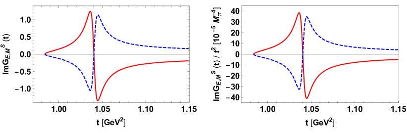
Figure 4: $K\bar{K}$ contribution through the anomalous coupling to the $\phi$ to the isoscalar spectral functions weighted with and without $1/t^{2}$. The red (solid) and blue (dashed) lines refer to the electric and magnetic form factors, $\text{Im}\leavevmode\nobreak\ G_{E}^{S}(t)$ and $\text{Im}\leavevmode\nobreak\ G_{M}^{S}(t)$, respectively.

The definitions of $\mathcal{J}_{\Lambda}(t)$, $\mathcal{J}_{\Sigma}(t)$ and $\mathcal{P}_{K}(t)$ can be found in Eq. (11). In Fig. 4, we show the $K\bar{K}$ loop contribution including the the one from the $\phi$-meson. To account for its finite width, we have substituted $M_{\phi}$ by $M_{\phi}-i\Gamma_{\phi}/2$, where $\Gamma_{\phi}\simeq 4\,$MeV is the width of the $\phi$. We find similar spectral functions for the electric and magnetic form factors except for the sign. Similar to Ref. [6], there is no enhancement on the left wing of the $\phi$ which sits directly at the $K\bar{K}$ threshold. Our results with vector mesons at one loop can, however, not directly be compared to dispersion-theoretical result of Ref. [7] as their calculation does not include all of the $\phi$-meson strength and ours would also require the inclusion of the NLO tensor coupling. Still, it is comforting to see that in the region of the $\phi$ there is little continuum strength. As noted earlier, the spectral functions generated by $K^{*}K$ and $K^{*}K^{*}$ start at much larger $t$ and turn out to be rather small, see Fig. 5 and Fig. 6, respectively.

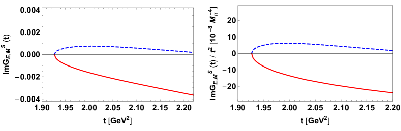
Figure 5: $K^{*}K$ contribution through the anomalous coupling to the $\phi$ to the isoscalar spectral functions weighted with and without $1/t^{2}$. For notations, see Fig. 4.

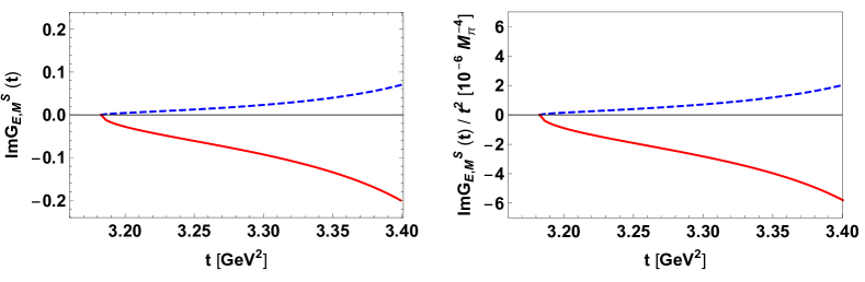
Figure 6: $K^{*}K^{*}$ contribution through the anomalous coupling to the $\phi$ to the isoscalar spectral functions weighted with and without $1/t^{2}$. For notations, see Fig. 4.

5 Summary

In this paper, we have used baryon chiral perturbation theory including vector mesons to derive new chiral constraints on the isoscalar electromagnetic spectral functions based on the leading order vector coupling. As noted earlier, the $\pi$-$\rho$ loop contribution is the most substantial non-resonant effect and needs to be included. The non-resonant $K\bar{K}$ contribution that sits under the $\phi$-meson is less pronounced, which is consistent with earlier findings, used e.g. in Ref. [2]. The inclusion of the tensor coupling effects should be considered next.

Appendix: A sample SU(3) calculation

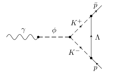
Figure 7: A Feynman diagram for the $\bar{K}K\Lambda$ loop contribution.

As an example for the pertinent SU(3) calculations, we consider the $K\bar{K}\Lambda$ contribution depicted in Fig. 7. The Feynman rules for the $\phi\gamma$, $\phi K^{+}K^{-}$, $\Lambda K^{-}p$ and $\Lambda K^{+}\bar{p}$ vertices appearing in this diagram are obtained as follows

$$\phi\gamma : \frac{2ieF_{V}}{3\sqrt{2}}(g^{\mu\nu}q^{2}-q^{\mu}q^{\nu})$$

$$\phi K^{+}K^{-} : 2(\partial^{\mu}K^{+})K^{-}\phi_{\mu}-2(\partial^{\mu}K^{-})K^{+}\phi_{\mu}$$

$$\qquad i\mathcal{L}\rightarrow 2ig(k_{1}^{\mu}-k_{2}^{\mu})$$

$$pK^{-}\bar{\Lambda} : -\frac{D}{2\sqrt{3}}\bar{\Lambda}(\partial^{\mu}K^{-})p-\frac{F\sqrt{3}}{2}\bar{\Lambda}(\partial^{\mu}K^{-})p$$

$$\qquad i\mathcal{L}\rightarrow\frac{(D+3F)}{2\sqrt{3}F_{\pi}}\gamma_{5}\not{k_{2}}$$

$$\Lambda K^{+}\bar{p} : -\frac{D}{2\sqrt{3}}\bar{p}(\partial^{\mu}K^{+})\Lambda-\frac{F\sqrt{3}}{2}\bar{p}(\partial^{\mu}K^{+})\Lambda$$

$$\qquad i\mathcal{L}\rightarrow\frac{(D+3F)}{2\sqrt{3}F_{\pi}}\gamma_{5}\not{k_{1}}$$

Here, $k_{1}$ and $k_{2}$ denote the momenta for the $K^{+}$ and the $K^{-}$, in order. The $\phi$ vector meson has momentum $q$ and Lorentz index $\mu$. The amplitude for the diagram in Fig. 7 reads

$$\Gamma^{\mu}(p_{i},p_{f},q) = \frac{egF_{V}(D+3F)^{2}}{24\sqrt{2}F_{\pi}^{2}\pi^{4}}$$

$$\times \mu^{4-n}\int d^{n}k\frac{(q^{\eta}q^{\mu}-q^{2}g^{\eta\mu})(2k^{\delta}-q^{\delta})(g_{\delta\eta}M_{\phi}^{2}-q_{\delta}q_{\eta})\gamma^{5}(\not{q}-\not{k})(\not{p_{i}}+\not{k}+m_{\Lambda})\gamma^{5}\not{k}}{(q^{2}-M_{\phi}^{2})(k^{2}-M_{K}^{2})((k+p_{i})^{2}-m_{\Lambda}^{2})((q-k)^{2}-M_{K}^{2})},$$

with $n$ the number of dimensions and $\mu$ the scale of dimensional regularization.

References

- [1] M. Hoferichter, B. Kubis, J. Ruiz de Elvira, H.-W. Hammer and U.-G. Meißner, Eur. Phys. J. A 52 (2016) no.11, 331 [arXiv:1609.06722 [hep-ph]].
- [2] M. A. Belushkin, H.-W. Hammer and U.-G. Meißner, Phys. Rev. C 75 (2007) 035202 [hep-ph/0608337].
- [3] V. Bernard, N. Kaiser and U.-G. Meißner, Nucl. Phys. A 611 (1996) 429 [hep-ph/9607428].
- [4] N. Kaiser and E. Passemar, arXiv:1901.02865 [nucl-th].
- [5] U.-G. Meißner, V. Mull, J. Speth and J. W. van Orden, Phys. Lett. B 408 (1997) 381 [hep-ph/9701296].
- [6] H. W. Hammer and M. J. Ramsey-Musolf, Phys. Rev. C 60 (1999) 045204 Erratum: [Phys. Rev. C 62 (2000) 049902] doi:10.1103/PhysRevC.60.045204, 10.1103/PhysRevC.62.049902 [hep-ph/9903367].
- [7] H. W. Hammer and M. J. Ramsey-Musolf, Phys. Rev. C 60 (1999) 045205 Erratum: [Phys. Rev. C 62 (2000) 049903]
- [8] L. L. Barz, H. Forkel, H. W. Hammer, F. S. Navarra, M. Nielsen and M. J. Ramsey-Musolf, Nucl. Phys. A 640 (1998) 259 [hep-ph/9803221].
- [9] B. Kubis and U.-G. Meißner, Nucl. Phys. A 679 (2001) 698 [hep-ph/0007056].
- [10] M. R. Schindler, J. Gegelia and S. Scherer, Eur. Phys. J. A 26 (2005) 1 [nucl-th/0509005].
- [11] P. Mergell, U.-G. Meißner and D. Drechsel, Nucl. Phys. A 596 (1996) 367 [hep-ph/9506375].
- [12] I. T. Lorenz, U.-G. Meißner, H.-W. Hammer and Y.-B. Dong, Phys. Rev. D 91 (2015) no.1, 014023 [arXiv:1411.1704 [hep-ph]].
- [13] S. Leupold, Eur. Phys. J. A 54 (2018) 1 [arXiv:1707.09210 [hep-ph]].
- [14] G. Ecker, J. Gasser, H. Leutwyler, A. Pich and E. de Rafael, Phys. Lett. B 223 (1989) 425.
- [15] G. Ecker, J. Gasser, A. Pich and E. de Rafael, Nucl. Phys. B 321, 311 (1989).
- [16] J. Gasser, M. E. Sainio and A. Svarc, Nucl. Phys. B 307 (1988) 779.
- [17] K. Nakayama, Y. Oh, J. Haidenbauer and T.-S. H. Lee, Phys. Lett. B 648, 351 (2007).
- [18] T. Bauer, J. C. Bernauer and S. Scherer, Phys. Rev. C 86 (2012) 065206.
- [19] D. Djukanovic, M. R. Schindler, J. Gegelia, G. Japaridze and S. Scherer, Phys. Rev. Lett. 93 (2004) 122002.
- [20] M. Bando, T. Kugo and K. Yamawaki, Phys. Rept. 164 (1988) 217.
- [21] U.-G. Meißner, Phys. Rept. 161 (1988) 213.
- [22] M. C. Birse, Z. Phys. A 355 (1996) 231.
- [23] B. Borasoy and U.-G. Meißner, Int. J. Mod. Phys. A 11 (1996) 5183.
- [24] A. Krause, Helv. Phys. Acta 63 (1990) 3.
- [25] A. Bramon, A. Grau and G. Pancheri, Phys. Lett. B 289 (1992) 97.
- [26] Y. Unal, A. Kucukarslan and S. Scherer, Phys. Rev. C 92 (2015) 055208 .
- [27] B. Borasoy, Phys. Rev. D 59 (1999) 054021.