Partial Label Learning with Self-Guided Retraining

Abstract

Partial label learning deals with the problem where each training instance is assigned a set of candidate labels, only one of which is correct. This paper provides the first attempt to leverage the idea of self-training for dealing with partially labeled examples. Specifically, we propose a unified formulation with proper constraints to train the desired model and perform pseudo-labeling jointly. For pseudo-labeling, unlike traditional self-training that manually differentiates the ground-truth label with enough high confidence, we introduce the maximum infinity norm regularization on the modeling outputs to automatically achieve this consideratum, which results in a convex-concave optimization problem. We show that optimizing this convex-concave problem is equivalent to solving a set of quadratic programming (QP) problems. By proposing an upper-bound surrogate objective function, we turn to solving only one QP problem for improving the optimization efficiency. Extensive experiments on synthesized and real-world datasets demonstrate that the proposed approach significantly outperforms the state-of-the-art partial label learning approaches.

Introduction

In partial label (PL) learning, each training example is represented by a single instance (feature vector) while associated with a set of candidate labels, only one of which is the ground-truth label. This learning paradigm is also termed as superset label learning (?; ?; ?; ?) or ambiguous label learning (?; ?; ?; ?). Since manually labeling the ground-truth label of each instance could incur unaffordable monetary or time cost, partial label learning has various application domains, such as web mining (?), image annotation (?; ?), and ecoinformatics (?).

Formally, let $\mathcal{X}\in\mathbb{R}^{n}$ be the $n$-dimensional feature space and $\mathcal{Y}=\{1,2,\cdots,l\}$ be the corresponding label space with $l$ labels. Suppose the PL training set is denoted by $\mathcal{D}=\{\mathbf{x}_{i},S_{i}\}_{i=1}^{m}$ where $\mathbf{x}_{i}\in\mathcal{X}$ is an $n$-dimensional feature vector and $S_{i}$ denotes the candidate label set. The key assumption of partial label learning lies in that the ground-truth label for $\mathbf{x}_{i}$ is concealed in its candidate label set $S_{i}$. The task of partial label learning is to learn a function $f:\mathcal{X}\rightarrow\mathcal{Y}$ from the PL training set $\mathcal{D}$, to correctly predict the label of a test instance.

Obviously, the available labeling information in the PL training set is ambiguous, as the ground-truth label is concealed in the candidate label set. Hence the key for accomplishing the task of learning from PL examples is how to disambiguate the candidate labels. Based on the employed strategy, existing approaches can be roughly grouped into two categories, including the average-based strategy and the identification-based strategy. The average-based strategy assumes that each candidate label makes equal contributions to the model training, and the prediction is made by averaging their modeling outputs (?; ?; ?). The identification-based strategy considers the ground-truth label as a latent variable, which is identified by an iterative refining procedure (?; ?; ?; ?). Although these approaches are able to extract the relative labeling confidence of each candidate label, they fail to reflect the mutually exclusive relationships among different candidate labels.

Motivated by self-training that takes into account such mutually exclusive relationships by directly labeling an unlabeled instance with enough high confidence, this paper gives the first attempt to leverage the similar idea to deal with PL instances. A straightforward method is to first apply a multi-output model on the PL examples, then pick up the candidate label with enough high confidence as the ground-truth label, finally retrain the model on the resulting data. This process is repeated until no PL examples exist, or no PL examples can be picked up as the ground-truth label. Although this method is intuitive, the model learned from PL examples are probably hard to directly identify the ground-truth label in accordance with the modeling outputs, as candidate label sets exist. Furthermore, the incorrectly identified labels could have contagiously negative impacts on the final predictions.

To address this problem, we propose a novel partial label learning approach named SURE (Self-gUided REtraining). Specifically, we propose a novel unified formulation with proper constraints to train the desired model and perform pseudo-labeling jointly. Unlike traditional self-training that manually differentiates the ground-truth label with enough high confidence, we introduce the maximum infinity norm regularization on the modeling outputs to automatically perform pseudo-labeling. In this way, the pseudo labels are decided by balancing the minimum approximation loss and the maximum infinity norm. To optimize the objective function, a convex-concave problem is encountered, as a result of the maximum infinity norm regularization. We show that solving this convex-concave problem is equivalent to solving a set of quadratic programming problems. By proposing an upper-bound surrogate objective function, we turn to solving only one quadratic programming problem for improving the optimization efficiency. Extensive experiments on a number of synthesized and real-world datasets clearly demonstrate the advantage of the proposed approach.

Related Work

Due to the difficulty in dealing with ambiguous labeling information of PL examples, there are only two general strategies to disambiguate the candidate labels, including the average-based strategy and the identification-based strategy.

The average-based strategy treats each candidate label equally in the model training phase. Following this strategy, some instance-based approaches predict the label $y$ of the test instance $\mathbf{x}$ by averaging the candidate labels of its neighbors (?; ?), i.e., $\operatorname*{arg\,max}_{y\in\mathcal{Y}}\sum_{\mathbf{x}_{i}\in{\mathcal{N}_{(\mathbf{x})}}}\mathbb{I}(y_{i}\in S_{i})$ where $\mathcal{N}(\mathbf{x})$ denotes the neighbors of instance $\mathbf{x}$. Besides, some parametric approaches adopt a parametric model $F(\mathbf{x}_{i},y;\theta)$ (?; ?) that differentiates the average modeling output of the candidate labels, i.e., $\frac{1}{|S_{i}|}\sum_{y\in S_{i}}F(\mathbf{x}_{i},y;\theta)$ from that of the non-candidate labels, i.e., $F(\mathbf{x}_{i},\hat{y};\theta)$ $(\hat{y}\in\hat{S}_{i})$, where $\hat{S}_{i}$ denotes the non-candidate label set. Although this strategy is intuitive, an obvious drawback is that the modeling output of the ground-truth label may be overwhelmed by the distractive outputs of the false positive labels.

The identification-based strategy considers the ground-truth label as a latent variable, and assumes certain parametric model $F(\mathbf{x},y;\theta)$ where the ground-truth label is identified by $\operatorname*{arg\,max}_{y\in S_{i}}F(\mathbf{x}_{i},y;\theta)$. Generally, the specific objective function is optimized on the basis of the maximum likelihood criterion: $\max(\sum_{i=1}^{m}\log(\sum_{y\in S_{i}}\frac{1}{|S_{i}|}F(\mathbf{x}_{i},y;\theta)))$ (?; ?) or the maximum margin criterion: $\max(\sum_{i=1}^{m}(\max_{y\in S_{i}}F(\mathbf{x}_{i},y;\theta)-\max_{\hat{y}\in\hat{S}_{i}}F(\mathbf{x}_{i},\hat{y};\theta)))$ (?; ?). One potential drawback of this strategy lies in that instead of recovering the ground-truth label, the differentiated label may turn out to be false positive, which could severely disrupt the subsequent model training.

Self-training is a commonly used technique for semi-supervised learning (?), which is characterized by the fact that the learning process uses its own predictions to teach itself. It has the advantage of taking into account the mutually exclusive relationships among labels by directly labeling an unlabeled instance with enough high confidence. Despite of its simplicity, the early mistakes could be exaggerated by further generating incorrectly labeled data. It is going to be even worse in the PL setting, as the ground-truth label is concealed in the candidate label set.

By alleviating the negative effects of self-training with a unified formulation, a novel partial label learning approach following the identification-based strategy will be introduced in the next section.

The Proposed Approach

Following the notations in Introduction, we denote by $\mathbf{X}=[\mathbf{x}_{1},\cdots,\mathbf{x}_{m}]^{\top}\in\mathbb{R}^{m\times n}$ the instance matrix and $\mathbf{Y}=[\mathbf{y}_{1},\cdots,\mathbf{y}_{m}]^{\top}\in\{0,1\}^{m\times l}$ the corresponding label matrix, where $y_{ij}=1$ means that the $j$-th label is a candidate label of the $i$-th instance $\mathbf{x}_{i}$, otherwise the $j$-th label is a non-candidate label. By adopting the identification-based strategy, we also regard the ground-truth label as latent variable, and denote by $\mathbf{P}=[\mathbf{p}_{1},\cdots,\mathbf{p}_{m}]^{\top}\in[0,1]^{m\times l}$ the confidence matrix where $p_{ij}$ represents the confidence (probability) of the $j$-th label being the ground-truth label of the $i$-th instance.

Unlike self-training that takes into account the mutually exclusive relationships among the candidate labels by performing deterministic pseudo-labeling, we introduce the maximum infinity norm regularization to automatically achieve this consideratum. A unified formulation with proper constraints is proposed as follows:

$$\min\sum_{i=1}^{m}(L(\mathbf{x}_{i},\mathbf{p}_{i},f)-\lambda\left\|\mathbf{p}_{i}\right\|_{\infty})+\beta\Omega(f)$$

$$\text{s.t.}\quad 0\leq p_{ij}\leq y_{ij},\ \forall i\in[m],\ \forall j\in[l]$$ (1)

$$\sum\nolimits_{j=1}^{l}p_{ij}=1,\quad\forall i\in[m]$$

where $[m]:=\{1,2,\cdots,m\}$, $L$ is the employed loss function, $\Omega$ controls the complexity of model $f$, and $\lambda,\beta$ are the tradeoff parameters. In this unified formulation, the model is learned from the pseudo label matrix $\mathbf{P}$, rather than the original noisy label matrix $\mathbf{Y}$. Besides, unlike the way of traditional self-training to perform deterministic pseudo-labeling by picking up the label with enough high confidence, the confidence of the ground-truth label is differentiated and enlarged by trading off the loss and the maximum infinity norm. Intuitively, only within the allowable range of loss, the candidate label with enough high confidence can be identified as the ground-truth label. In this way, the negative effects of self-training is alleviated by training the model and performing pseudo-labeling jointly. In addition, the first constraint plays two roles: the confidence of each candidate label should be larger than 0, but no more than 1; the confidence of each non-candidate label should be strictly 0. The second constraint guarantees that each confidence vector $\mathbf{p}_{i}$ will always be in the probability simplex, i.e., $\{\mathbf{p}_{i}\in[0,1]^{l}:\sum_{j}p_{ij}=1|i\in[m]\}$. This constraint also implicitly takes into consideration the mutually exclusive relationships among the candidate labels, as the confidence of certain one candidate label is enlarged by the maximum infinity norm regularization, the confidences of other candidate labels will be naturally reduced.

To instantiate the above formulation, we adopt the widely used squared loss, i.e., $L(\mathbf{x}_{i},\mathbf{p}_{i},f)=\left\|f(\mathbf{x}_{i})-\mathbf{p}_{i}\right\|_{2}^{2}$. Besides, we employ the simple linear model $f(\mathbf{x}_{i})=\mathbf{W}^{\top}\mathbf{x}_{i}+\mathbf{b}$ where $\mathbf{W},\mathbf{b}$ are model parameters. A kernel extension for the general nonlinear case will be introduced in the later section. To control the model parameter, we simply adopt the common squared Frobenius norm of $\mathbf{W}$, i.e., $\left\|\mathbf{W}\right\|_{F}^{2}$. To sum up, the final optimization problem is presented as follows:

$$\min\limits_{\mathbf{P},\mathbf{W},\mathbf{b}}\sum_{i=1}^{m}(\left\|\mathbf{W}^{\top}\mathbf{x}_{i}+\mathbf{b}-\mathbf{p}_{i}\right\|_{2}^{2}-\lambda\left\|\mathbf{p}_{i}\right\|_{\infty})+\beta\left\|\mathbf{W}\right\|_{F}^{2}$$

$$\text{s.t.}\quad 0\leq p_{ij}\leq y_{ij},\ \forall i\in[m],\ \forall j\in[l]$$ (2)

$$\sum\nolimits_{j=1}^{l}p_{ij}=1,\quad\forall i\in[m]$$

Optimization

Problem (2) can be solved by alternating minimization, which enable us to optimize one variable with other variables fixed. This process is repeated until convergence or the maximum number of iterations is reached.

Updating $\mathbf{W}$ and $\mathbf{b}$

With $\mathbf{P}$ fixed, problem (2) with respective to $\mathbf{W}$ and $\mathbf{b}$ can be compactly stated as follows:

$$\min\limits_{\mathbf{W},\mathbf{b}}\left\|\mathbf{X}\mathbf{W}+\mathbf{1}\mathbf{b}^{\top}-\mathbf{P}\right\|_{F}^{2}+\beta\left\|\mathbf{W}\right\|_{F}^{2}$$ (3)

where $\mathbf{1}$ denotes the vector with all components set to 1. Setting the gradient with respect to $\mathbf{W}$ and $\mathbf{b}$ to 0, the closed-form solutions can be easily obtained:

$$\mathbf{W} =(\mathbf{X}^{\top}\mathbf{X}+\beta\mathbf{I}-\frac{\mathbf{X}^{\top}\mathbf{1}\mathbf{1}^{\top}\mathbf{X}}{m})^{-1}(\mathbf{X}^{\top}\mathbf{P}-\frac{\mathbf{X}^{\top}\mathbf{1}\mathbf{1}^{\top}\mathbf{P}}{m})$$

$$\mathbf{b} =\frac{1}{m}(\mathbf{P}^{\top}\mathbf{1}-\mathbf{W}^{\top}\mathbf{X}^{\top}\mathbf{1})$$ (4)

Kernel Extension

To deal with the nonlinear case, the above linear learning model can be easily extended to a kernel-based nonlinear model. To achieve this, we utilize a feature mapping $\phi(\cdot):\mathbb{R}^{n}\rightarrow\mathbb{R}^{\mathcal{H}}$ to map the original feature space $\mathbf{x}\in\mathbb{R}^{n}$ to some higher (maybe infinite) dimensional Hilbert space $\phi(\mathbf{x})\in\mathbb{R}^{\mathcal{H}}$. By representor theorem (?), $\mathbf{W}$ can be represented by a linear combination of input variables, i.e., $\mathbf{W}=\phi(\mathbf{X})^{\top}\mathbf{A}$ where $\mathbf{A}\in\mathbb{R}^{m\times l}$ stores the combination weights of instances. Hence $\phi(\mathbf{X})\mathbf{W}=\mathbf{K}\mathbf{A}$ where $\mathbf{K}\in\phi(\mathbf{X})\phi(\mathbf{X})^{\top}\in\mathbb{R}^{m\times m}$ is the kernel matrix with each element defined by $k_{ij}=\phi(\mathbf{x}_{i})^{\top}\phi(\mathbf{x}_{j})=\kappa(\mathbf{x}_{i},\mathbf{x}_{j})$, and $\kappa(\cdot,\cdot)$ denotes the kernel function. In this paper, Gaussian kernel function $\kappa(\mathbf{x}_{i},\mathbf{x}_{j})=\exp(-\left\|\mathbf{x}_{i}-\mathbf{x}_{j}\right\|_{2}^{2}/(2\sigma^{2}))$ is employed with $\sigma$ set to the averaged pairwise distances of instances. By incorporating such kernel extension, problem (3) can be presented as follows:

$$\min\limits_{\mathbf{A},\mathbf{b}}\left\|\mathbf{K}\mathbf{A}+\mathbf{1}\mathbf{b}^{\top}-\mathbf{P}\right\|_{F}^{2}+\beta\operatorname{tr}(\mathbf{A}^{\top}\mathbf{K}\mathbf{A})$$ (5)

where $\operatorname{tr}(\cdot)$ is the trace operator. Setting the gradient with respect to $\mathbf{A}$ and $\mathbf{b}$ to 0, the closed-form solutions are reported as:

$$\mathbf{A} =(\mathbf{K}+\beta\mathbf{I}-\frac{\mathbf{1}\mathbf{1}^{\top}\mathbf{K}}{m})^{-1}(\mathbf{P}-\frac{\mathbf{1}\mathbf{1}^{\top}\mathbf{P}}{m})$$

$$\mathbf{b} =\frac{1}{m}(\mathbf{P}^{\top}\mathbf{1}-\mathbf{A}^{\top}\mathbf{K}^{\top}\mathbf{1})$$ (6)

By adopting this kernel extension, we choose to update the parameters $\mathbf{A}$ and $\mathbf{b}$ throughout this paper.

Updating $\mathbf{P}$

With $\mathbf{A}$ and $\mathbf{b}$ fixed, the modeling output matrix $\mathbf{Q}=[\mathbf{q}_{1},\cdots,\mathbf{q}_{m}]^{\top}\in\mathbb{R}^{m\times l}$ is denoted by $\mathbf{Q}=\phi(\mathbf{X})\mathbf{W}+\mathbf{1}\mathbf{b}^{\top}=\mathbf{K}\mathbf{A}+\mathbf{1}\mathbf{b}^{\top}$, problem (2) reduces to:

$$\min\limits_{\mathbf{P}}\sum_{i=1}^{m}(\left\|\mathbf{p}_{i}-\mathbf{q}_{i}\right\|_{2}^{2}-\lambda\left\|\mathbf{p}_{i}\right\|_{\infty})$$

$$\text{s.t.}\quad 0\leq p_{ij}\leq y_{ij},\ \forall i\in[m],\ \forall j\in[l]$$ (7)

$$\sum\nolimits_{j=1}^{l}p_{ij}=1,\quad\forall i\in[m]$$

Obviously, we can solve problem (7) by solving $m$ independent problems, one for each example. We further denote by OP the minimum loss of the problem for the $i$-th example:

$$\textsl{OP}=\min\limits_{\mathbf{p}_{i}}\left\|\mathbf{p}_{i}-\mathbf{q}_{i}\right\|_{2}^{2}-\lambda\left\|\mathbf{p}_{i}\right\|_{\infty}$$

$$\text{s.t.}\quad\mathbf{1}^{\top}\mathbf{p}_{i}=1$$ (8)

$$\quad\mathbf{0}\leq\mathbf{p}_{i}\leq\mathbf{y}_{i}$$

Here, problem (8) is a constrained convex-concave problem, as the first term is convex while the second term is concave. Instead of using traditional time-consuming convex-concave procedure (?) to solve this problem, we show that optimizing this problem is equivalent to solving $l$ independent QP problems, each for one label. We denoted by $\textsl{OPI}(j)$ the minimum loss of the problem for the $j$-th label:

$$\textsl{OPI}(j)=\min\limits_{\mathbf{p}_{i}}\left\|\mathbf{p}_{i}-\mathbf{q}_{i}\right\|_{2}^{2}-\lambda p_{ij}$$

$$\text{s.t.}\quad p_{ik}\leq p_{ij},\ \forall k\in[l]$$ (9)

$$\quad\mathbf{1}^{\top}\mathbf{p}_{i}=1$$

$$\quad\mathbf{0}\leq\mathbf{p}_{i}\leq\mathbf{y}_{i}$$

Theorem 1.

$\textsl{OP}=\min\nolimits_{j\in[l]}\textsl{OPI}(j)$.

Proof.

It is obvious that there must exist $j\in[l]$ such that $p_{ij}=\left\|\mathbf{p}_{i}\right\|_{\infty}$ and the optimum loss OP of problem (8) can be obtained. In addition, if $p_{ij}=\left\|\mathbf{p}_{i}\right\|_{\infty}$ coincidentally holds, then $\textsl{OPI}(j)=\textsl{OP}$, as in such case, problem (9) is equivalent to problem (8). While if $p_{ij}\neq\left\|\mathbf{p}_{i}\right\|_{\infty}$, then $\textsl{OPI}(j)>\textsl{OP}$. Hence $\textsl{OP}=\min\nolimits_{j\in[l]}\textsl{OPI}(j)$. ∎

Theorem 1 gives us a motivation to solve problem (8) by selecting the minimum loss from $l$ independent quadratic programming problems. However, this may be time-consuming, as the label space could be very large. Thus, we propose a surrogate objective function to upper bound the loss incurred by problem (8). Specifically, we select the candidate label $j$ with the maximal modeling output by $j=\operatorname*{arg\,max}_{j\in S_{i}}q_{ij}$ where $S_{i}$ is the candidate label set containing the indices of candidate labels of the instance $\mathbf{x}_{i}$. The proposed surrogate objective function is given as:

$$\textsl{OPS}=\min\limits_{\mathbf{p}_{i}}\left\|\mathbf{p}_{i}-\mathbf{q}_{i}\right\|_{2}^{2}-\lambda p_{ij}$$

$$\text{s.t.}\quad q_{ik}\leq q_{ij},\ \forall k\in S_{i},\ \exists j\in S_{i}$$ (10)

$$\quad p_{ik}\leq p_{ij},\ \forall k\in[l]$$

$$\quad\mathbf{1}^{\top}\mathbf{p}_{i}=1$$

$$\quad\mathbf{0}\leq\mathbf{p}_{i}\leq\mathbf{y}_{i}$$

Note that the difference between problem (10) and problem (9) lies in that problem (10) adds a constraint to select the label $j$ with the maximal modeling output. Unlike problem (9) that considers the possibility of each label being the ground-truth label, problem (10) directly assumes the candidate label $j$ with the maximal modeling output $j=\operatorname*{arg\,max}_{j\in S_{i}}q_{ij}$ to be the label that is most likely the ground-truth label. This assumption coincides with self-training, which also considers the label with the maximal modeling output as the ground-truth label. Different from self-training that manually performs deterministic pseudo-labeling, our approach aims to automatically enlarge the confidence of the label with the maximal modeling output as much as possible by balancing the two terms in problem (10). In this way, we not only avoid the opinionated mistakes by self-training, but also take into account the mutually exclusive relationships among candidate labels.

Theorem 2.

$\textsl{OP}\leq\textsl{OPS}$.

Proof.

From the formulation of problem (10) and problem (9), it is easy to see that $\textsl{OPS}\in\{\textsl{OPI}(j)|j\in S_{i}\}$. Since $S_{i}\subset[l]$, $\textsl{OPS}\in\{\textsl{OPI}(j)|j\in[l]\}$. Which means, $\min_{j\in[l]}\textsl{OPI}(j)\leq\textsl{OPS}$. Using Theorem (1), $\textsl{OP}=\min_{j\in[l]}\textsl{OPI}(j)\leq\textsl{OPS}$. ∎

Theorem (2) shows that OPS of problem (10) is an upper bound of the loss OP incurred by problem (8). Hence we can choose to optimize problem (10) for efficiency, as only one QP problem is involved. Such problem can be easily solved by any off-the-shelf QP tools.

After the completion of the optimization process, the predicted label $\widetilde{y}$ of the text instance $\widetilde{\mathbf{x}}$ is given as:

$$\widetilde{y}=\operatorname*{arg\,max}\limits_{j\in[l]}\sum_{i=1}^{m}a_{ij}\kappa(\widetilde{\mathbf{x}},\mathbf{x}_{i})+b_{j}$$ (11)

The pseudo code of SURE is presented in Algorithm 1.

Algorithm 1 The SURE Algorithm

0:  $\mathcal{D}$: the PL training set $\mathcal{D}=\{(\mathbf{X},\mathbf{Y})\}$$\lambda,\beta$: the regularization parameters$\widetilde{\mathbf{x}}$: the unseen test instance

0:  $\widetilde{y}$: the predicted label for the test instance $\widetilde{\mathbf{x}}$

0:  

1:  construct the kernel matrix $\mathbf{K}=[\kappa(\mathbf{x}_{i},\mathbf{x}_{j})]_{m\times m}$;

2:  initialize $\mathbf{P}=\mathbf{Y}$;

3:  repeat

4:     update $\mathbf{A}=[a_{ij}]_{m\times l}$ and $\mathbf{b}=[b_{j}]_{l}$ according to (6);

5:     update $\mathbf{Q}=\mathbf{KA}+\mathbf{1}\mathbf{b}^{\top}$;

6:     calculate $\mathbf{P}$ by solving (10) with a general QP procedure for each training example;

7:  until convergence or the maximum number of iterations.

8:  return the predicted label $\widetilde{y}$ according to (11).

Experiments

Comparing Algorithms

To demonstrate the effectiveness of SURE, we conduct extensive experiments to compare SURE with six state-of-the-art partial label learning algorithms, each configured with suggested parameters according to the respective literature:

• PLKNN (?): a $k$-nearest neighbor approach that makes predictions by averaging the labeling information of neighboring examples [suggested configuration: $k\in\{5,6,\cdots,10\}$];

• CLPL (?): a convex formulation that deals with PL examples by transforming partial label learning problem to binary learning problem via feature mapping [suggested configuration: SVM with squared hinge loss];

• IPAL (?): an instance-based approach that disambiguates candidate labels by an adapted label propagation scheme. [suggested configuration: $\alpha\in\{0,0.1,\cdots,1\}$, $k\in\{5,6,\cdots,10\}$];

• PLSVM (?): a maximum margin approach that learns from PL examples by optimizing margin-based objective function [suggested configuration: $\lambda\in\{10^{-3},10^{-2},\cdots,10^{3}\}$];

• PALOC (?): an approach that adapts one-vs-one decomposition strategy to enable binary decomposition for learning from PL examples [suggested configuration: $\mu=10$];

• LSBCMM (?): a maximum likelihood approach that learns from PL examples via mixture models [suggested configuration: $L=\lceil 10\log_{2}(l)\rceil$].

The two parameters $\lambda$ and $\beta$ for SURE are chosen from $\{0.001,0.01,0.05,0.1,0.3,0.5,1\}$. Parameters for each algorithm are selected by five-fold cross-validation on the training set. For each dataset, ten-fold cross-validation is performed where mean prediction accuracies and the standard deviations are recorded. In addition, we use $t$-test at 0.05 significance level for two independent samples to investigate whether SURE is significantly superior/inferior (win/loss) to the comparing algorithms for all the experiments.

Controlled UCI Datasets

The characteristics of 4 controlled UCI datasets are reported in Table 1. Following the widely-used controlling protocol (?; ?; ?; ?; ?; ?), each UCI dataset can be used to generate artificial partial label datasets. There are three controlling parameters $p$, $r$ and $\epsilon$ where $p$ controls the proportion of PL examples, $r$ controls the number of false positive labels, and $\epsilon$ controls the probability of a specific false positive label occurring with the ground-truth label. As shown in Table 1, there are 4 configurations, each corresponding to 7 results. Hence we can totally generate $4\times 4\times 7=112$ different artificial partial label datasets.

Figure 1 shows the classification accuracy of each algorithm as $\epsilon$ ranges from 0.1 to 0.7 when $p=0.1$ and $r=1$ (Configuration (I)). In this setting, a specific label is selected as the coupled label that co-occurs with the ground-truth label with probability $\epsilon$, and any other label would be randomly chosen to be a false positive label with probability $1-\epsilon$. Figures 2, 3, and 4 illustrate the classification accuracy of each algorithm as $p$ ranges from 0.1 to 0.7 when $r=1,2$, and 3 (Configuration (II), (III), and (IV)), respectively. In these three settings, $r$ extra labels are randomly chosen to be the false positive labels. That is, the number of candidate labels for each instance is $r+1$.

Table 1: Characteristics of the controlled UCI datasets.

Dataset	deter	ecoli	glass	usps
Examples	358	336	214	9298
Features	23	7	9	256
Labels	6	8	6	10

Configurations:
(I) $p=0.1,r=1$, $\epsilon\in\{0.1,0.2,\cdots,0.7\}$
(II) $r=1$, $p\in\{0.1,0.2,\cdots,0.7\}$
(III) $r=2$, $p\in\{0.1,0.2,\cdots,0.7\}$
(IV) $r=3$, $p\in\{0.1,0.2,\cdots,0.7\}$

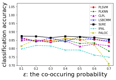
(a) ecoli

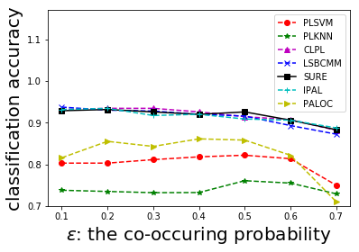
(b) deter

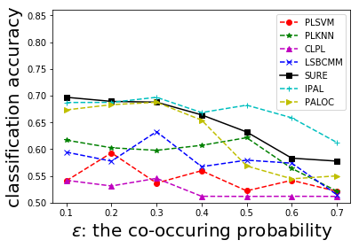
(c) glass

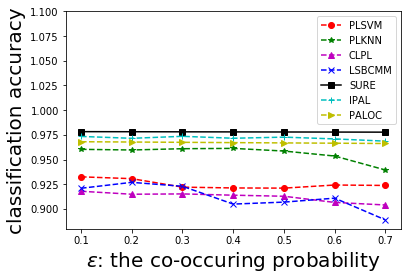
(d) usps

Figure 1: Classification performance on controlled UCI datasets with $\epsilon$ ranging from 0.1 to 0.7 ($p=1,r=1$).

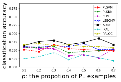
(a) ecoli

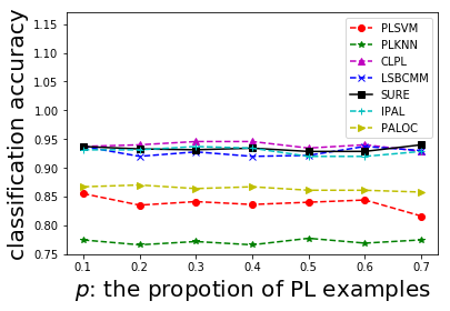
(b) deter

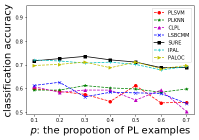
(c) glass

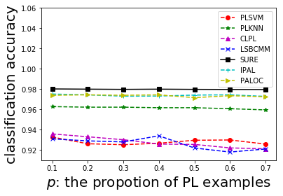
(d) usps

Figure 2: Classification performance on controlled UCI datasets with $p$ ranging from 0.1 to 0.7 ($r=1$).

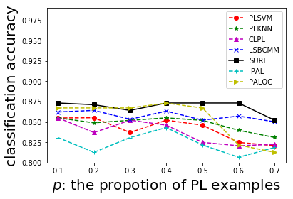
(a) ecoli

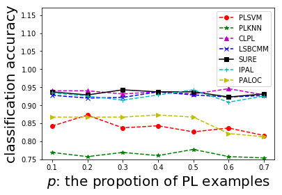
(b) deter

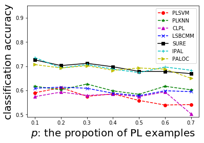
(c) glass

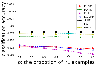
(d) usps

Figure 3: Classification performance on controlled UCI datasets with $p$ ranging from 0.1 to 0.7 ($r=2$).

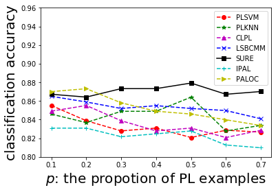
(a) ecoli

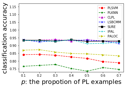
(b) deter

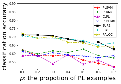
(c) glass

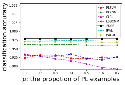
(d) usps

Figure 4: Classification performance on controlled UCI datasets with $p$ ranging from 0.1 to 0.7 ($r=3$).

As shown in Figures 1, 2, 3, and 4, SURE outperforms other comparing algorithms in general. To further statistically compare SURE with other algorithms, the detailed win/tie/loss counts between SURE and the comparing algorithms are recorded in Table 2. Out of the 112 results, it is easy to observe that:

• SURE achieves superior or at least comparable performance against PLKNN and PLSVM in all cases.

• SURE achieves superior performance against CLPL and LSCMM in 72.3% and 58.9% cases while outperformed by them in only 4.5% and 1.8% cases, respectively.

• SURE outperforms IPAL and PALOC in 50.9% and 63.4% cases while outperformed by them in only 5.4% and 2.7% cases, respectively.

In summary, the effectiveness of SURE on controlled UCI datasets is demonstrated.

Table 2: Win/tie/loss ($t$-test at 0.05 significance level for two independent samples) counts on the controlled UCI datasets between SURE and the comparing algorithms.

	PLKNN	CLPL	IPAL	PLSVM	PALOC	LSBCMM
(I)	24/4/0	21/6/1	14/11/3	21/7/0	20/8/0	14/14/0
(II)	24/4/0	19/7/2	15/13/0	24/4/0	17/10/1	17/10/1
(III)	24/4/0	21/6/1	14/13/1	25/3/0	17/10/1	19/9/0
(IV)	25/3/0	20/7/1	14/12/2	27/1/0	17/10/1	16/11/1
Total	97/15/0	81/26/5	57/49/6	97/15/0	71/38/3	66/44/2

Table 3: Characteristics of real-world partial label datasets.

Dataset	Examples	Features	Labels	Avg. CLs	Task Domain
Lost	1122	108	16	2.23	automatic face naming (?)
MSRCv2	1758	48	23	3.16	object classification (?)
Soccer Player	17472	279	171	2.09	automatic face naming (?)
Yahoo! News	22991	163	219	1.91	automatic face naming (?)
FG-NET	1002	262	78	7.48	facial age estimation (?)

Table 4: Classification accuracy of each algorithm on the real-world datasets. Furthermore, $\bullet$/$\circ$ indicates whether SURE is statistically superior/inferior to the comparing algorithm ($t$-test at 0.05 significance level for two independent samples).

	SURE	PLKNN	CLPL	IPAL	PLSVM	PALOC	LSBCMM
Lost	0.781$\pm$0.039	0.432$\pm$0.051$\bullet$	0.742$\pm$0.038$\bullet$	0.678$\pm$0.053$\bullet$	0.729$\pm$0.042$\bullet$	0.629$\pm$0.056$\bullet$	0.693$\pm$0.035$\bullet$
MSRCv2	0.515$\pm$0.027	0.417$\pm$0.034$\bullet$	0.413$\pm$0.041$\bullet$	0.529$\pm$0.039	0.461$\pm$0.046$\bullet$	0.479$\pm$0.042$\bullet$	0.473$\pm$0.037$\bullet$
Soccer Player	0.533$\pm$0.017	0.495$\pm$0.018$\bullet$	0.368$\pm$0.010$\bullet$	0.541$\pm$0.016	0.464$\pm$0.011$\bullet$	0.537$\pm$0.015	0.498$\pm$0.017$\bullet$
Yahoo! News	0.644$\pm$0.015	0.483$\pm$0.011$\bullet$	0.462$\pm$0.009$\bullet$	0.609$\pm$0.011$\bullet$	0.629$\pm$0.010$\bullet$	0.625$\pm$0.005$\bullet$	0.645$\pm$0.005
FG-NET	0.078$\pm$0.021	0.039$\pm$0.018$\bullet$	0.063$\pm$0.027	0.054$\pm$0.030$\bullet$	0.063$\pm$0.029	0.065$\pm$0.019	0.059$\pm$0.025$\bullet$
FG-NET(MAE3)	0.458$\pm$0.024	0.269$\pm$0.045$\bullet$	0.458$\pm$0.022	0.362$\pm$0.034$\bullet$	0.356$\pm$0.022$\bullet$	0.435$\pm$0.018$\bullet$	0.382$\pm$0.029$\bullet$
FG-NET(MAE5)	0.615$\pm$0.019	0.438$\pm$0.053$\bullet$	0.596$\pm$0.017$\bullet$	0.540$\pm$0.033$\bullet$	0.479$\pm$0.016$\bullet$	0.609$\pm$0.043	0.532$\pm$0.038$\bullet$

Real-World Datasets

Table 3 reports the characteristics of real-world partial label datasets including Lost (?), MSRCv2 (?), Soccer Player (?), Yahoo! News (?), and FG-NET (?). These real-world partial label datasets are from several task domains. For automatic face naming (Lost, Soccer Player, and Yahoo! News), each face (instance) is cropped from an image or a video frame, and the names appearing on the corresponding captions or subtitles are taken as candidate labels. For facial age estimation (FG-NET), human faces are regarded as instances while ages annotated by crowdsourcing labelers serve as candidate labels. For object classification (MSRCv2), each image segment is considered as an instance, and objects appearing in the same image are taken as candidate labels. The average number of candidate labels (Avg. CLs) per instance is also reported in Table 3.

Table 4 reports the mean classification accuracy as well as the standard deviation of each algorithm on each real-world dataset. Note that the average number of candidate labels (Avg. CLs) of FG-NET dataset is quite large, which results in an extremely low classification accuracy of each algorithm. For better evaluation of this facial age estimation task, we employ conventional mean absolute error (MAE) (?) to conduct two extra experiments. Specifically, for FG-NET (MAE3/MAE5), a test example is considered correctly classified if the MAE between the predicted age and the ground-truth age is no more than 3/5 years. As shown in Table 4, we can observe that:

• SURE significantly outperforms PLKNN on all the real-world datasets.

• Out of the 42 cases (6 comparing algorithms and 7 datasets), SURE significantly outperforms all the comparing algorithms in 78.6% cases, and achieves competitive performance in 21.4% cases.

• It is worth noting that SURE is never significantly outperformed by any comparing algorithms.

These experimental results on real-world datasets also demonstrate the effectiveness of SURE.

Further Analysis

Parameter Sensitivity Analysis

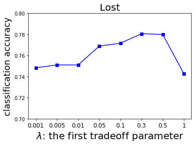
(a) Varying $\lambda$ on Lost

(b) Varying $\beta$ on Lost

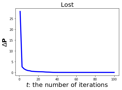
(c) Convergence on Lost

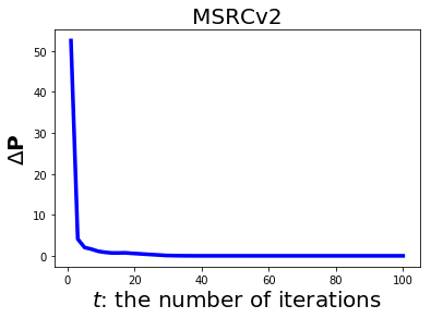
(d) Convergence on MSRCv2

Figure 5: Parameter sensitivity and convergence analysis for SURE. (a) Sensitivity analysis of $\lambda$ on Lost; (b) Sensitivity analysis of $\beta$ on MSRCv2; (c) Convergence analysis on Lost; (d) Convergence analysis on MSRCv2.

There are two tradeoff parameters $\lambda$ and $\beta$ for SURE, which should be manually searched in advance. Hence this section studies how $\lambda$ and $\beta$ influence the prediction accuracy produced by SURE. We vary one parameter, while keeping the other fixed at the best setting. Figures 5(a) and 5(b) show the performance of SURE on the Lost dataset given different values of $\lambda$ and $\beta$ respectively. Note that $\lambda$ controls the importance of the maximum infinity norm regularization. When $\lambda$ is very small, the mutually exclusive relationships among labels are hardly considered, thus the classification accuracy would be at a low level. As $\lambda$ increases, we start to take into consideration such exclusive relationships, and the classification accuracy increases. However, if $\lambda$ is sufficiently large, the classification accuracy will drop dramatically. This is because when we overly concentrate on the mutually exclusive relationships among labels, we will directly regard the candidate label that has the maximal modeling output as the ground-truth label. Since to maximize the infinity norm $\left\|\mathbf{p}\right\|_{\infty}$ is overly important, the approximation loss will be totally ignored. From the above, we can draw a conclusion that it would be better to balance the approximation loss and the mutually exclusive relationships among labels. Such conclusion clearly comfirms the effectiveness of the SURE approach. Another tradeoff parameter $\beta$ aims to control the model complexity. The classification accuracy curve of varying $\beta$ obviously accords with our cognition that it is important to balance between overfitting and underfitting.

Illustration of Convergence

We illustrate the convergece of SURE by using the difference of the optimization variable $\mathbf{P}$ between two successive iterations ($\Delta\mathbf{P}=\left\|\mathbf{P}^{(t+1)}-\mathbf{P}^{(t)}\right\|_{F}$). Figure 5(c) and 5(d) show the convergence curves of SURE on Lost and MSRCv2 respectively. It is apparent that $\Delta\mathbf{P}$ gradually decreases to 0 as the number of iterations $t$ increases. Hence the convergence of SURE is demonstrated.

Conclusion

In this paper, we utilize the idea of self-training to exaggerate the mutually exclusive relationships among candidate labels for further enhancing partial label learning performance. Instead of manually performing pseudo-labeling after model training, we propose a unified formulation (named SURE) with the maximum infinity norm regularization to train the desired model and perform pseudo-labeling jointly. Extensive experimental results demonstrate the effectiveness of SURE.

Since self-training is a typical semi-supervised learning method, it would be interesting to extend SURE to the setting of semi-supervised learning. Besides, as mutually exclusive relationships exist in general multi-class problems, it would be valuable to explore other possible ways to incorporate such relationships into partial label learning.

References

- [Chen et al. 2014] Chen, Y.-C.; Patel, V. M.; Chellappa, R.; and Phillips, P. J. 2014. Ambiguously labeled learning using dictionaries. IEEE Transactions on Information Forensics and Security 9(12):2076–2088.
- [Chen, Patel, and Chellappa 2017] Chen, C.-H.; Patel, V. M.; and Chellappa, R. 2017. Learning from ambiguously labeled face images. IEEE Transactions on Pattern Analysis and Machine Intelligence.
- [Cour, Sapp, and Taskar 2011] Cour, T.; Sapp, B.; and Taskar, B. 2011. Learning from partial labels. Journal of Machine Learning Research 12(5):1501–1536.
- [Feng and An 2018] Feng, L., and An, B. 2018. Leveraging latent label distributions for partial label learning. In Proceedings of the 27th International Joint Conference on Artificial Intelligence, 2107–2113.
- [Gong et al. 2018] Gong, C.; Liu, T.; Tang, Y.; Yang, J.; Yang, J.; and Tao, D. 2018. A regularization approach for instance-based superset label learning. IEEE Transactions on Cybernetics 48(3):967–978.
- [Guillaumin, Verbeek, and Schmid 2010] Guillaumin, M.; Verbeek, J.; and Schmid, C. 2010. Multiple instance metric learning from automatically labeled bags of faces. Lecture Notes in Computer Science 63(11):634–647.
- [Hüllermeier and Beringer 2006] Hüllermeier, E., and Beringer, J. 2006. Learning from ambiguously labeled examples. Intelligent Data Analysis 10(5):419–439.
- [Hüllermeier and Cheng 2015] Hüllermeier, E., and Cheng, W. 2015. Superset learning based on generalized loss minimization. In Joint European Conference on Machine Learning and Knowledge Discovery in Databases, 260–275.
- [Jin and Ghahramani 2003] Jin, R., and Ghahramani, Z. 2003. Learning with multiple labels. In Advances in Neural Information Processing Systems, 921–928.
- [Liu and Dietterich 2012] Liu, L.-P., and Dietterich, T. G. 2012. A conditional multinomial mixture model for superset label learning. In Advances in Neural Information Processing Systems, 548–556.
- [Liu and Dietterich 2014] Liu, L.-P., and Dietterich, T. 2014. Learnability of the superset label learning problem. In International Conference on Machine Learning, 1629–1637.
- [Luo and Orabona 2010] Luo, J., and Orabona, F. 2010. Learning from candidate labeling sets. In Advances in Neural Information Processing Systems, 1504–1512.
- [Nguyen and Caruana 2008] Nguyen, N., and Caruana, R. 2008. Classification with partial labels. In Proceedings of the 14th ACM SIGKDD International Conference on Knowledge Discovery and Data Mining, 551–559.
- [Panis and Lanitis 2014] Panis, G., and Lanitis, A. 2014. An overview of research activities in facial age estimation using the fg-net aging database. In European Conference on Computer Vision, 737–750.
- [Schölkopf, Smola, and others 2002] Schölkopf, B.; Smola, A. J.; et al. 2002. Learning with kernels: support vector machines, regularization, optimization, and beyond. MIT press.
- [Wang and Zhang 2018] Wang, J., and Zhang, M.-L. 2018. Towards mitigating the class-imbalance problem for partial label learning. In Proceedings of the 24th ACM SIGKDD Conference on Knowledge Discovery and Data Mining, 2427–2436.
- [Wu and Zhang 2018] Wu, X., and Zhang, M.-L. 2018. Towards enabling binary decomposition for partial label learning. In Proceedings of the 27th International Joint Conference on Artificial Intelligence, 2427–2436.
- [Yu and Zhang 2016] Yu, F., and Zhang, M.-L. 2016. Maximum margin partial label learning. In Proceedings of Asian Conference on Machine Learning, 96–111.
- [Yuille and Rangarajan 2003] Yuille, A. L., and Rangarajan, A. 2003. The concave-convex procedure. Neural Computation 15(4):915–936.
- [Zeng et al. 2013] Zeng, Z.-N.; Xiao, S.-J.; Jia, K.; Chan, T.-H.; Gao, S.-H.; Xu, D.; and Ma, Y. 2013. Learning by associating ambiguously labeled images. In Proceedings of the IEEE Conference on Computer Vision and Pattern Recognition, 708–715.
- [Zhang and Yu 2015] Zhang, M.-L., and Yu, F. 2015. Solving the partial label learning problem: An instance-based approach. In Proceedings of the 24th International Joint Conference on Artificial Intelligence, 4048–4054.
- [Zhang, Zhou, and Liu 2016] Zhang, M.-L.; Zhou, B.-B.; and Liu, X.-Y. 2016. Partial label learning via feature-aware disambiguation. In Proceedings of the 22nd ACM SIGKDD International Conference on Knowledge Discovery and Data Mining, 1335–1344.
- [Zhu and Goldberg 2009] Zhu, X., and Goldberg, A. B. 2009. Introduction to semi-supervised learning. Synthesis Lectures on Artificial Intelligence and Machine Learning 3(1):1–130.