Fourier Neural Networks: A Comparative Study

Abstract

We review neural network architectures which were motivated by Fourier series and integrals and which are referred to as Fourier neural networks. These networks are empirically evaluated in synthetic and real-world tasks. Neither of them outperforms the standard neural network with sigmoid activation function in the real-world tasks. All neural networks, both Fourier and the standard one, empirically demonstrate lower approximation error than the truncated Fourier series when it comes to approximation of a known function of multiple variables.

1 Introduction

Over the past few years, neural networks have re-emerged as powerful machine-learning models, yielding state-of-the-art results in fields such as computer vision, speech recognition, and natural language processing. In this work we explore several neural network architectures, the authors of which were inspired by Fourier series and integrals. Such architectures will be collectively referred to as Fourier Neural Networks (FNNs). First FNNs were proposed in 80s and 90s, but they are not widely used nowadays. Is there any reasonable explanation for this, or were they simply not given enough attention? To answer this question we perform empirical evaluation of the FNNs, found in the existing literature, on synthetic and real-world datasets. We are mainly interested in the following hypotheses: Is any of the FNNs superior to others? Does any FNN outperform conventional feedforward neural network with the logistic sigmoid activation? Our experiments show that the FNN of Gallant and White (1988) outperforms all other FNNs, and that all FNNs are not better than the standard feedforward neural architecture with sigmoid activation function except the case of modeling synthetic data.

2 Preliminaries

Notation. We let $\mathbb{Z}$ and $\mathbb{R}$ denote the integer and real numbers, respectively. Bold-faced letters ($\mathbf{x}$, $\mathbf{y}$) denote vectors in $d$-dimensional Euclidean space $\mathbb{R}^{d}$, and plain-faced letters ($x$, $f$) denote either scalars or functions. $\langle\cdot,\cdot\rangle$ denotes inner product: $\langle\mathbf{x},\mathbf{y}\rangle:=\sum_{j=1}^{d}x_{j}y_{j}$; and $\|\cdot\|$, $\|\cdot\|_{2}$ denote the Euclidean norm: $\|\mathbf{x}\|:=\|\mathbf{x}\|_{2}:=\sqrt{\langle\mathbf{x},\mathbf{x}\rangle}$.

Feedforward Neural Networks. Following a standard convention, we define a feedforward neural network with one hidden layer of size $n$ on inputs in $\mathbb{R}^{d}$ as

$$\mathbf{x}\mapsto v_{0}+\sum_{k=1}^{n}v_{k}\sigma(\langle\mathbf{x},\mathbf{w}_{k}\rangle+b_{k})$$ (1)

where $\sigma(\cdot)$ is the activation function, and $v_{k},b_{k}\in\mathbb{R}$, $\mathbf{w}_{k}\in\mathbb{R}^{d}$, $k=1,\ldots,n$, are parameters of the network. The universal approximation theorem (Hornik et al. (1989); Cybenko (1989)) states that a feedforward network (1) with any “squashing” activation function $\sigma(\cdot)$, such as the logistic sigmoid function, can approximate any Borel measurable function $f(\mathbf{x})$ with any desired non-zero amount of error, provided that the network is given enough hidden layer size $n$. Universal approximation theorems have also been proved for a wider class of activation functions, which includes the now commonly used $\mathrm{ReLU}$ (Leshno et al. (1993)). The neural network (1) with logistic sigmoid activation $\sigma(x):=1/(1+e^{-x})$ is referred to as standard or vanilla feedforward neural network.

Fourier Series. Let $f(\mathbf{x})$ be a function integrable in the $d$-dimensional cube $[-\pi,\pi]^{d}$. The Fourier series of the function $f(\mathbf{x})$ is the series

$$\sum_{\mathbf{k}\in\mathbb{Z}^{d}}\hat{f}_{\mathbf{k}}e^{i\langle\mathbf{x},\mathbf{k}\rangle},$$ (2)

where the numbers $\hat{f}_{\mathbf{k}}$, called Fourier coefficients, are defined by

$$\hat{f}_{\mathbf{k}}:=(2\pi)^{-d}\underset{[-\pi,\pi]^{d}}{\int}f(\mathbf{y})e^{-i\langle\mathbf{y},\mathbf{k}\rangle}d\mathbf{y},$$

Conceptually, the feedforward neural network with one hidden layer (1) and the partial sum of the Fourier series (2) are similar in a sense that both are linear combinations of non-linear transformations of the input $\mathbf{x}$. The major differences between them are as follows:

• The Fourier series has a direct access to the function $f(\mathbf{x})$ being approximated, whereas the neural network does not have it — instead it is usually given a training set of pairs $\{\mathbf{x}_{i},f(\mathbf{x}_{i})+\epsilon_{i}\}$, where $\epsilon_{i}$ is a noise (error).

• The coefficients and linear transformations of the input in the Fourier series are fixed, but they are trainable in the neural network and are subject to estimation based on the training set $\{\mathbf{x}_{i},f(\mathbf{x}_{i})+\epsilon_{i}\}$.

There exists a variety of results on convergence of different types of partial sums (rectangular, square, spherical) of the multiple Fourier series (2) to $f(\mathbf{x})$ in various senses (uniform, mean, almost everywhere). We refer the reader to the works of Alimov et al. (1976) and Alimov et al. (1977) for a survey of such results. It seems that the existence of such convergence guarantees has motivated several authors to design the activation functions for (1) in such a way that the resulting neural networks mimic the behavior of the Fourier series (2). In the next section we give a brief overview of such networks.

3 Fourier Neural Networks

FNN of Gallant and White (1988): The earliest attempt on making a neural network resemble the Fourier series is due to Gallant and White (1988) who have suggested the “cosine squasher”

$$\sigma_{\rm GW}(x):=\begin{cases}0,&x\in(-\infty,-\frac{\pi}{2}),\\ \frac{1}{2}\left(\cos\left(x+\frac{3\pi}{2}\right)+1\right),&x\in[-\frac{\pi}{2},\frac{\pi}{2}],\\ 1,&x\in(\frac{\pi}{2},+\infty),\end{cases}$$ (3)

as an activation function in the feedforward network (1). Moreover, they show that when additionally the connections $\mathbf{w}_{i}$, $b_{i}$ from input to hidden layer are hardwired in a special way, the obtained feedforward network yields a Fourier series approximation to a given function $f(\mathbf{x})$. Thus, such networks possess all the approximation properties of Fourier series representations. In particular, approximation to any desired accuracy of any square integrable function can be achieved by such a network, using sufficiently many hidden units. McCaffrey and Gallant (1994) showed that the squared approximation error for sufficiently smooth functions is of order $O(n^{-1})$, where $n$ is the network’s hidden layer size. We notice here that Barron (1993) has established the same order of the approximation error for the feedforward networks with any sigmoidal activation and when the function being approximated $f(\mathbf{x})$ has a bound on the first moment of the magnitude distribution of the Fourier transform. FNN of Gallant and White (1988) is denoted as $f_{\rm GW}$.

FNN of Silvescu (1999): Another attempt to mimic the behavior of the Fourier series by a neural network was done by Silvescu (1999), who introduced the following FNN:

$$f_{\rm S}:\mathbf{x}\mapsto v_{0}+\sum_{k=1}^{n}v_{k}\sigma_{\rm S}(\mathbf{x};\boldsymbol{\omega}_{k},\boldsymbol{\phi}_{k}),$$ (4)

with

$$\sigma_{\rm S}(\mathbf{x};\boldsymbol{\omega}_{k},\boldsymbol{\phi}_{k}):=\prod_{j=1}^{d}\cos(\omega_{kj}x_{j}+\phi_{kj}),$$ (5)

where $\boldsymbol{\omega}_{k},\boldsymbol{\phi}_{k}\in\mathbb{R}^{d}$, $v_{k}\in\mathbb{R}$ are trainable parameters. As we can see, Silvescu’s FNN (4) does not follow the framework of the standard feedforward neural networks (1), and moreover its activation function is not sigmoidal. Figure 1 depicts the difference between (1) and (4) for the case when $d=3$ and $n=2$.

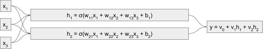
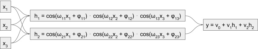
Figure 1: Standard feedforward NN (top) vs Silvescu’s Fourier NN (bottom). In the standard NN non-linearity is applied on top of the linear transformation of the whole input, whereas in the Silvescu’s network non-linearity is applied separately to each component of the input vector.

Because of this difference, the result of Barron (1993) is not applicable to Silvescu’s FNN. However, we conjecture that the same convergence rate is valid for the Silvescu’s FNN. The proof (or disproof) of this conjecture is deferred to our future work.

FNN of Liu (2013): More recently, several authors suggested the following architecture

$$f_{\rm L}:\mathbf{x}\mapsto v_{0}+\sum_{k=1}^{n}v_{k}\cos(\langle\mathbf{w}_{k},\mathbf{x}\rangle+b_{k})+u_{k}\sin(\langle\mathbf{p}_{k},\mathbf{x}\rangle+q_{k}),$$ (6)

where $\mathbf{w}_{k},\mathbf{p}_{k}\in\mathbb{R}^{d}$, $b_{k},q_{k}\in\mathbb{R}$ are either hardwired or trainable, and $v_{k},u_{k}\in\mathbb{R}$ are trainable parameters. Tan (2006) explored aircraft engine fault diagnostics using (6), Zuo and Cai (2005), Zuo and Cai (2008), Zuo et al. (2009) used it for the control of a class of uncertain nonlinear systems. The above-mentioned authors did not provide rigorous mathematical analysis of this architecture, instead they used it as an ad-hoc solution in their engineering tasks. Although this FNN fits into the general feedforward framework (1), its activations are not sigmoidal, and thus the result of Barron (1993) is not applicable here as well. Liu (2013) empirically evaluated (6) on various datasets and showed that in certain cases it converges faster than the feedforward network with sigmoid activation and has equally good predicting accuracy and generalization ability. Also, only in the work of Liu (2013) all the weights in (6) are allowed to be trainable, hence we refer to this architecture as $f_{\rm L}$.

4 Empirical Evaluation

In this section we will perform empirical evaluation of the Fourier neural networks $f_{\rm GW}$, $f_{\rm S}$, $f_{\rm L}$ from Section 3 against vanilla feedforward network (1) with sigmoid activation on synthetic and real-world datasets. By “synthetic datasets” we mean datasets generated from a known function. In this case we can also compare the performance of Fourier neural networks to the approximation error given by the partial Fourier series.

4.1 Synthetic tasks

We try to approximate a function of one variable $x\mapsto|x|$, $x\in[-\pi,\pi]$, and a function of $d=100$ variables: $\mathbf{x}\mapsto\mathbb{I}[\|\mathbf{x}\|\leq 1]$, $\mathbf{x}\in\{\mathbf{x}\in\mathbb{R}^{100}:\,\|\mathbf{x}\|\leq 2\}$, where $\mathbb{I}[\cdot]$ is the indicator function. In both cases we sampled $5\cdot 10^{5}$ data instances uniformly from the domains of the functions. To each instance, we associated a target value according to the target function $|x|$ or $\mathbb{I}[\|\mathbf{x}\|\leq 1]$. Another $10\cdot 10^{4}$ examples were generated in a similar manner, of which $5\cdot 10^{4}$ examples were used as a validation set, and $5\cdot 10^{4}$ examples were used as a test set. We trained 32 networks on these datasets: for each of the above-mentioned models (vanilla feedforward network, $f_{\rm GW}$, $f_{\rm S}$, $f_{\rm L}$) we varied the hidden layer size from 100 to 800 with the step 100. Training was performed with Adam optimizer (Kingma and Ba (2015)). We used the squared loss $l(y,\hat{y}):=(y-\hat{y})^{2}$ and batches of size 100. For each model, a learning rate was tuned separately on the validation set. The results are presented in Figure 2.

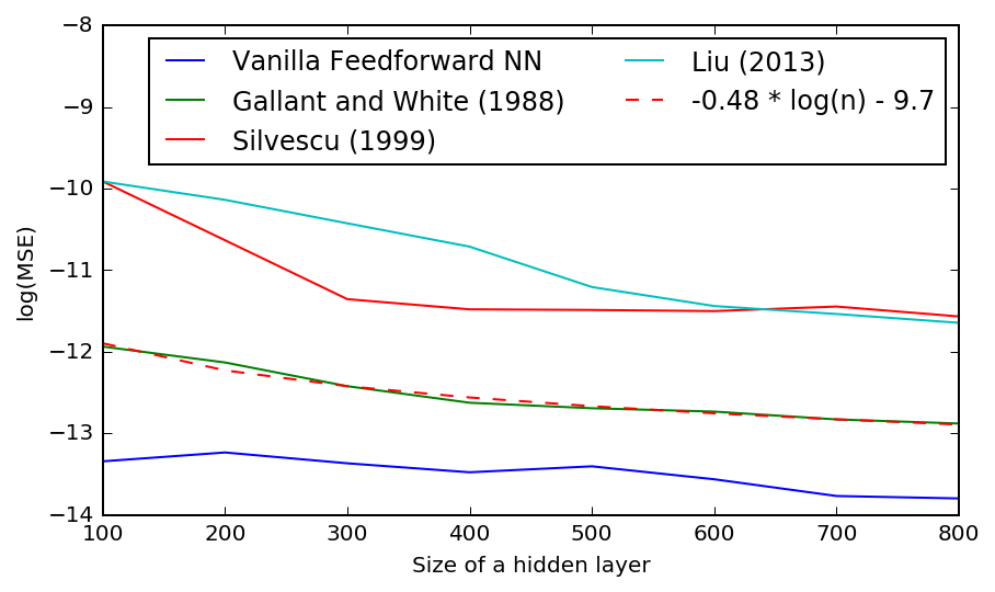
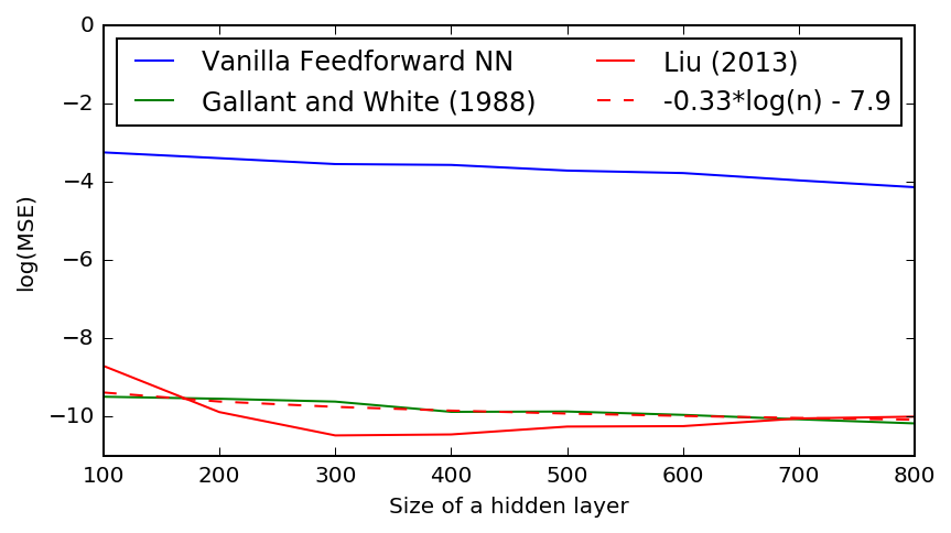
Figure 2: Results of approximating $|x|$ (left) and $\mathbb{I}[\|\mathbf{x}\|\leq 1]$ (right) by Fourier neural networks and Fourier series. MSE stands for the mean squared error, $\frac{1}{T}\sum_{i=1}^{T}(y_{i}-\hat{y}_{i})^{2}$. Dashed curves were obtained by regressing $\log(\mathrm{MSE})$ of $f_{\rm GW}$ on $\log n$. ^∗Evaluation of $f_{\rm S}$ for the indicator function data is in progress.

Vanilla feedforward network (1) obtains lowest mean squared error (MSE) for $|x|$, whereas the FNN of Gallant and White (1988) outperforms all other models for $\mathbb{I}[\|\mathbf{x}\|\leq 1]$. According to the regression fits (dashed curves in Fig. 2), the function $x\mapsto|x|$ is approximated by the neural networks with error $O(n^{-0.48})$, and this is much worse than the approximation error given by the partial sums of the Fourier series of $f(x)=|x|$, which, according to Lemma 1 below, is of order $O(n^{-3})$. For the function $\mathbf{x}\mapsto\mathbb{I}[\|\mathbf{x}\|\leq 1]$ results are to other way around: the approximation error by the neural networks is of order $O(n^{-0.33})$, while it is of the order $O(n^{-1/100})$ by the truncated Fourier series (see Lemma 2 below). We keep in mind that the theoretical result of Barron (1993) states that for any function from a certain class (to which the indicator function does belong) a feedforward neural network with one hidden layer of size $n$ will be able to approximate this function with a squared error of order $O(n^{-1})$. We are not guaranteed, however, that the training algorithm will be able to learn that function. Even if the neural network is able to represent the function, learning can fail, since the optimization algorithm used for training may not be able to find the value of the parameters that corresponds to the desired function. We attribute the mismatch, $O(n^{-1/3})$ instead of $O(n^{-1})$, between the orders of approximation errors to the suboptimal estimation of the parameters of the networks by the Adam optimizer. However, in general we have experimentally confirmed Barron’s claim that neural networks with $n$ hidden units can approximate functions with much smaller error than series expansions with $n$ terms.

We also notice here that directly comparing neural networks with truncated Fourier series is somewhat unfair, as these are two different categories of approximation: Fourier series serve as some theoretical reference, which is possible only when we have access to the function being approximated.

Lemma 1.

For the $2\pi$-periodic function $f(x):=|x|$, $x\in[-\pi,\pi]$, let $S_{n}(x)$ be the $n^{\text{th}}$ partial sum of its Fourier series. Then, for some constant $C$,

$$\|f-S_{n}\|_{2}^{2}\leq\frac{C}{n^{3}}.$$ (7)

Proof.

The Fourier series expansion of $f$ is given by

$$f(x)=\frac{\pi}{2}+\sum_{k=1}^{\infty}a_{k}\cos(2k-1)x,\qquad a_{k}:=-\frac{4}{\pi}\frac{1}{(2k-1)^{2}},$$ (8)

(see Example 1, p. 23, from Folland (1992)), and therefore by Parseval’s Theorem,

$$\|f-S_{n}\|_{2}^{2} :=\int_{-\pi}^{\pi}(f(x)-S_{n}(x))^{2}dx=\pi\sum_{k=n+1}^{\infty}{a_{k}^{2}}$$

$$\leq\pi\sum_{k=n+1}^{\infty}\Big{(}-\frac{4}{\pi}\frac{1}{(2k-1)^{2}}\Big{)}^{2}=\frac{16}{\pi}\sum_{k=n+1}^{\infty}\frac{1}{(2k-1)^{4}}.$$ (9)

Since $(2k-1)^{-4}$ is a monotonically decreasing sequence, we have

$$\int_{n+1}^{\infty}\frac{du}{(2u-1)^{4}}\leq\sum_{k=n+1}^{\infty}\frac{1}{(2k-1)^{4}}\leq\int_{n}^{\infty}\frac{du}{(2u-1)^{4}},$$

that is,

$$\frac{1}{6(2n+1)^{3}}\leq\sum_{k=n+1}^{\infty}\frac{1}{(2k-1)^{4}}\leq\frac{1}{6(2n-1)^{3}}.$$ (10)

Combining (9) and (10) we obtain (7). ∎

Lemma 2.

Let $\mathbf{x}\in[-\pi,\pi]^{d}$ and $f(\mathbf{x})$ be the indicator function of the unit ball in $\mathbb{R}^{d}$, that is, $f(\mathbf{x}):=\mathbb{I}[\mathbf{x}\leq 1]$. Let $S_{R}(\mathbf{x})$ be the truncated Fourier Series of $f(\mathbf{x})$, where $R\geq 1$ is the radius of the partial spherical summation and $n$ is the number of terms in the partial sum. Then, for some dimensional dependent constant $C_{d}$, the following holds

$$\|f-S_{R}\|^{2}_{2}\leq\frac{C_{d}}{n^{1/d}}.$$ (11)

Proof.

For $\mathbf{x}\in\mathbb{R}^{d}$, denote $\|\mathbf{x}\|_{1}:=|x_{1}|+\ldots+|x_{d}|$, and $\|\mathbf{x}\|_{\infty}:=\max_{1\leq i\leq d}|x_{i}|$. It is known that

$$\|\mathbf{x}\|_{2}\leq\|\mathbf{x}\|_{1}\leq\sqrt{d}\|\mathbf{x}\|_{2},\quad\|\mathbf{x}\|_{\infty}\leq\|\mathbf{x}\|_{1}\leq d\|\mathbf{x}\|_{\infty},$$ (12)

which in particular implies

$$\|\mathbf{x}\|_{\infty}\geq\frac{1}{d}\|\mathbf{x}\|_{1}\geq\frac{1}{d}\|\mathbf{x}\|_{2}.$$ (13)

From (12) and (13) it follows that

$$\{\mathbf{k}\in\mathbb{Z}^{d}:\,\|\mathbf{k}\|_{2}>R\}\subset\{\mathbf{k}\in\mathbb{Z}^{d}:\,\|\mathbf{k}\|_{\infty}>R/d\},$$ (14)

and, therefore,

$$\sum_{\|\mathbf{k}\|_{2}>R}\frac{1}{\|\mathbf{k}\|^{d+1}_{2}}\leq\sum_{\|\mathbf{k}\|_{\infty}>R/d}\frac{1}{\|\mathbf{k}\|_{2}^{d+1}}\lesssim\sum_{\|\mathbf{k}\|_{\infty}>R/d}\frac{1}{\|\mathbf{k}\|_{1}^{d+1}}.$$ (15)

Here “$A\lesssim B$” means that “$A\leq C_{d}B$”, for some dimensional dependent constant $C_{d}$. Analogously, we write “$A\sim B$” if “$A\lesssim B$” and “$B\lesssim A$”. Denoting $\tilde{R}:=R/d$, we obtain the following decomposition

$$\{\|\mathbf{k}\|_{\infty}>\tilde{R}\}\\ =\bigcup_{1\leq j\leq d}\bigcup_{1\leq i_{1}\neq\dots\neq i_{d}\leq d}\Big{\{}|k_{i_{\alpha}}|>\tilde{R},\,1\leq\alpha\leq j;\\ |k_{i_{\alpha}}|\leq\tilde{R},\,j<\alpha\leq d\Big{\}}.$$

Thus the latter sum in (15) can be estimated as follows,

$$\sum_{\|\mathbf{k}\|_{\infty}>\tilde{R}}\frac{1}{\|\mathbf{k}\|_{1}^{d+1}}=\sum_{\|\mathbf{k}\|_{\infty}>\tilde{R}}\frac{1}{(\|\mathbf{k}\|_{1}^{(d+1)/j})^{j}}$$

$$\leq\sum_{j=1}^{d}\sum_{1\leq i_{1}\neq\dots\neq i_{d}\leq d}\sum_{|k_{i_{1}}|>\tilde{R}}\cdots\sum_{|k_{i_{j}}|>\tilde{R}}\sum_{|k_{i_{j+1}}|\leq\tilde{R}}\cdots\sum_{|k_{i_{d}}|\leq\tilde{R}}$$

$$\qquad\times\frac{1}{|k_{i_{1}}|^{(d+1)/j}\cdots|k_{i_{j}}|^{(d+1)/j}}$$

$$\lesssim\sum_{j=1}^{d}\tilde{R}^{d-j}\Big{(}\sum_{|\ell|>\tilde{R}}\frac{1}{|\ell|^{(d+1)/j}}\Big{)}^{j}\sim\sum_{j=1}^{d}\tilde{R}^{d-j}\Big{(}\int_{\tilde{R}}^{\infty}\frac{du}{u^{(d+1)/j}}\Big{)}^{j}$$

$$\sim\sum_{j=1}^{d}\frac{\tilde{R}^{d-j}}{\tilde{R}^{d+1-j}}\sim\frac{1}{\tilde{R}}\sim\frac{1}{R}.$$ (16)

Combining (15) and (16) we get

$$\sum_{\|\mathbf{k}\|_{2}>R}\frac{1}{\|\mathbf{k}\|^{d+1}_{2}}\lesssim\frac{1}{R}.$$ (17)

Let $\mathrm{SE}$ denote the squared error in the left-hand side of (11). Then, Parseval’s Theorem allows us to write

$$\mathrm{SE} :=\int_{[-\pi,\pi]^{d}}|f(\mathbf{x})-S_{R}(\mathbf{x})|^{2}\,d\mathbf{x}=\int_{[-\pi,\pi]^{d}}\Big{|}\sum_{\|\mathbf{k}\|_{2}>R}\hat{f}_{\mathbf{k}}e^{i\mathbf{k}\cdot\mathbf{x}}\Big{|}^{2}d\mathbf{x}$$

$$=(2\pi)^{d}\sum_{\|\mathbf{k}\|_{2}>R}|\hat{f}_{\mathbf{k}}|^{2}.$$

Using the estimates of the Fourier coefficients for the indicator function of a ball (Pinsky et al. (1993), p. 120), and denoting $\alpha:=\|\mathbf{k}\|_{2}-(d-1)\pi/4$, we get

$$\mathrm{SE} =(2\pi)^{d}\sum_{\|\mathbf{k}\|_{2}>R}\Big{[}\frac{C_{d}}{\|\mathbf{k}\|_{2}^{(d+1)/2}}\Big{\{}\sin\alpha+O\Big{(}\frac{1}{\sqrt{\|\mathbf{k}\|_{2}}}\Big{)}\Big{\}}\Big{]}^{2}$$

$$\sim\sum_{\|\mathbf{k}\|_{2}>R}\frac{1}{\|\mathbf{k}\|_{2}^{d+1}}\Big{[}\sin^{2}\alpha+2\sin\alpha\,O\Big{(}\frac{1}{\sqrt{\|\mathbf{k}\|_{2}}}\Big{)}+O\Big{(}\frac{1}{\|\mathbf{k}\|_{2}}\Big{)}\Big{]}$$

$$\lesssim\sum_{\|\mathbf{k}\|_{2}>R}\frac{1}{\|\mathbf{k}\|_{2}^{d+1}}.$$ (18)

From (17) and (18) it follows that

$$\mathrm{SE}\lesssim\frac{1}{R}.$$ (19)

The number of terms $n$ in the spherical partial sum $S_{R}(\mathbf{x})$ is equal to the number of integer points in the $d$-ball of radius $R$, which is, according to Götze (2004), approximated by the volume of such ball up to an error $O(R^{d-2})$, i.e.

$$n\sim R^{d}.$$

Combining this with (19), we get $\mathrm{SE}\lesssim n^{-1/d}$. ∎

4.2 Image recognition

We performed evaluation of the FNNs in the image recognition task using the MNIST dataset (LeCun et al. (1998)), which is commonly used for training various image processing systems. It consists of handwritten digit images, $28\times 28$ pixels in size, organized into 10 classes (0 to 9) with 60,000 training and 10,000 test samples. Portion of training samples was used as validation data. Images were represented as vectors in $\mathbb{R}^{784}$, hidden layer size was fixed at 64 for all networks, and classification was done based on the softmax normalization. Training was performed with Adam optimizer (Kingma and Ba (2015)). We used the cross-entropy loss and batches of size 100. Learning rate was tuned separately for each model on the validation data. Table 2 compares classification accuracy obtained by the models.

Model	Accuracy	Learning rate
Vanilla feedforward NN	0.9648	0.0096
FNN of Gallant and White (1988)	0.9695	0.0045
FNN of Silvescu (1999)	0.9659	0.0134
FNN of Liu (2013)	0.9638	0.0034

Table 1: Evaluation of the networks on MNIST data.

As we can see, all the networks demonstrate similar performance in this task. In fact, the differences between accuracy results are not significant across the models, Pearson’s Chi-square test of independence $\chi^{2}_{3}=5.6449$, $p$-value $>0.1$.

4.3 Language modeling

A statistical language model (LM) is a model which assigns a probability to a sequence of words. Below we specify one type of such models based on the structurally constrained recurrent network (SCRN) of Mikolov et al. (2015).

Let $\mathcal{W}$ be a finite vocabulary of words. We assume that words have already been converted into indices. Let $\mathbf{E}\in\mathbb{R}^{|\mathcal{W}|\times d_{\mathcal{W}}}$ be an input embedding matrix for words — i.e., it is a matrix in which the $w$th row (denoted as $\mathbf{w}$) corresponds to an embedding of the word $w\in\mathcal{W}$. Based on word embeddings $\mathbf{w_{1:k}}=\mathbf{w_{1}},\ldots,\mathbf{w_{k}}$ for a sequence of words $w_{1:k}$, the SCRN model produces two sequences of states, $\mathbf{s_{1:k}}$ and $\mathbf{h_{1:k}}$, according to the equations

$$\mathbf{s_{t}}=(1-\alpha)\mathbf{w_{t}}\mathbf{B}+\alpha\mathbf{s_{t-1}},$$ (20)

$$\mathbf{h_{t}}=\sigma(\mathbf{w_{t}}\mathbf{A}+\mathbf{s_{t}}\mathbf{P}+\mathbf{h_{t-1}}\mathbf{R}),$$ (21)

where $\mathbf{B}\in\mathbb{R}^{|\mathcal{W}|\times d_{s}}$, $\mathbf{A}\in\mathbb{R}^{|\mathcal{W}|\times d_{h}}$, $\mathbf{P}\in\mathbb{R}^{d_{s}\times d_{h}}$, $\mathbf{R}\in\mathbb{R}^{d_{h}\times d_{h}}$, $d_{s}$ and $d_{h}$ are dimensions of $\mathbf{s_{t}}$ and $\mathbf{h_{t}}$, $\sigma(\cdot)$ is the logistic sigmoid function. The last couple of states $(\mathbf{s_{k}},\mathbf{h_{k}})$ is assumed to contain information on the whole sequence $w_{1:k}$ and is further used for predicting the next word $w_{k+1}$ of a sequence according to the probability distribution

$$\Pr(w_{k+1}|w_{1:k})=\operatorname{softmax}(\mathbf{s_{k}}\mathbf{U}+\mathbf{h_{k}}\mathbf{V}),$$ (22)

where $\mathbf{U}\in\mathbb{R}^{d_{s}\times|\mathcal{W}|}$ and $\mathbf{V}\in\mathbb{R}^{d_{h}\times|\mathcal{W}|}$ are output embedding matrices. For the sake of simplicity we omit bias terms in (21) and (22). Being conceptually much simpler, the SCRN architecture demonstrates performance comparable to the widely used LSTM model in language modeling task (Kabdolov et al. (2018)), and this is why we chose it for our experiments.

We train and evaluate the SCRN model for $(d_{h},d_{s})$ $\in\{(40,10)$, $(90,10)$, $(100,40)$, $(300,40)\}$ on the PTB (Marcus et al. (1993)) data set, for which the standard training (0-20), validation (21-22), and test (23-24) splits along with pre-processing per Mikolov et al. (2010) is utilized. We replace $\sigma$ in (21) with $\sigma_{\rm GW}$, $\sigma_{\rm S}$, and $\sigma_{\rm L}$ defined in Section 3, and we refer to such modification as Fourier layers. The choice of hyperparameters is guided by the work of Kabdolov et al. (2018), except that for the Fourier layers we additionally tune the learning rate, its decay schedule and the initialization scale over the validation split. To evaluate the performance of the language models we use perplexity (PPL) over the test set. The results are provided in Table 2.

Activation	(40, 10)	(90, 10)	(100, 40)	(300, 40)
$\sigma$	128.0	118.6	118.7	120.6
$\sigma_{\rm GW}$	132.8	119.6	120.1	127.9
$\sigma_{\rm S}$	144.4	133.4	127.7	125.9
$\sigma_{\rm L}$	165.7	139.3	147.5	156.8

Table 2: Evaluation of the SCRN language models on the PTB data. Columns 2–5 correspond to different configurations of the hidden ($d_{h}$) and context ($d_{s}$) states sizes.

As one can see, the conventional sigmoid activation outperforms all Fourier activations, and, as in the case of synthetic data, the Fourier layer of Gallant and White (1988) is better than other Fourier layers for most of the architectures.

5 Discussion

The FNNs of Silvescu (1999) (4) and of Liu (2013) (6) have non-sigmoidal activations, which makes their optimization more difficult. Although the activation function of $f_{\mathrm{GW}}(\cdot)$ is sigmoidal, it still underperforms the standard feedforward neural network in almost all cases. We hypothesize that this is because $\sigma_{\mathrm{GW}}$ is constant outside $\left[-\frac{\pi}{2},\frac{\pi}{2}\right]$, while $\sigma(x)=1/(1+e^{-x})$ is never constant. This means that $\forall x_{1},\,x_{2}\in(\pi/2,\infty)$: $\sigma_{\mathrm{GW}}(x_{1})=\sigma_{\mathrm{GW}}(x_{2})$, i.e. the activation of Gallant and White (1988) (3) does not distinguish between any values to the right from $\pi/2$ (and to the left from $-\pi/2$). The standard sigmoid activation $\sigma(\cdot)$, on the other hand, can theoretically distinguish between any pair $x_{1},\,x_{2}\in\mathbb{R}$: $x_{1}\neq x_{2}$. To see whether the constant behavior of $\sigma_{\mathrm{GW}}$ indeed causes problems, we look at the pre-activated values $x\cdot w+b$ for $x$ from the validation split in the synthetic task of approximating $x\mapsto|x|$, $x\in[-\pi,\pi]$. The histogram of these pre-activated values for the $f_{\mathrm{GW}}$ with hidden layer size $n=100$ is given in Figure 3.

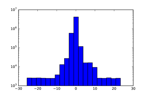
Figure 3: Histogram of pre-activated values ($x\cdot w+b$) in the FNN of Gallant and White (1988). Frequencies are at log-scale.

It turns out that $\approx 8\%$ of pre-activated values are outside of $[-\pi/2,\pi/2]$, and this information is lost when filtered through $\sigma_{\mathrm{GW}}$.

6 Conclusion and Future Work

All Fourier neural networks are not better than the standard neural network with sigmoid activation except when it comes to modeling synthetic data. The architecture of Gallant and White (1988) is the best among Fourier neural networks. When the function being approximated is known and depends on multiple variables, the neural networks with just one hidden layer may provide much better approximation compared to truncated Fourier series.

In this paper we focused on neural architectures with one hidden layer. It is interesting to compare Fourier neural networks in a multilayer setup. We defer such study to our future work which will also include experiments with a larger variety of functions, as well as mathematical analysis of the approximation of Barron functions by Silvescu’s and Liu’s Fourier neural networks.

Compliance with ethical standards

Conflict of Interest. The authors declare that they have no conflict of interest.

References

- Alimov et al. [1976] Sh A Alimov, Vladimir Aleksandrovich Il’in, and Evgenii Mikhailovich Nikishin. Convergence problems of multiple trigonometric series and spectral decompositions. i. Russian Mathematical Surveys, 31(6):29, 1976.
- Alimov et al. [1977] Sh A Alimov, Vladimir Aleksandrovich Il’in, and Evgenii Mikhailovich Nikishin. Problems of convergence of multiple trigonometric series and spectral decompositions. ii. Russian Mathematical Surveys, 32(1):115–139, 1977.
- Barron [1993] Andrew R Barron. Universal approximation bounds for superpositions of a sigmoidal function. IEEE Transactions on Information theory, 39(3):930–945, 1993.
- Cybenko [1989] George Cybenko. Approximation by superpositions of a sigmoidal function. Mathematics of control, signals and systems, 2(4):303–314, 1989.
- Folland [1992] Gerald B Folland. Fourier analysis and its applications, volume 4. American Mathematical Soc., 1992.
- Gallant and White [1988] A Ronald Gallant and Halbert White. There exists a neural network that does not make avoidable mistakes. In Proceedings of the Second Annual IEEE Conference on Neural Networks, San Diego, CA, I, 1988.
- Götze [2004] Friedrich Götze. Lattice point problems and values of quadratic forms. Inventiones mathematicae, 157(1):195–226, 2004.
- Hornik et al. [1989] Kurt Hornik, Maxwell Stinchcombe, and Halbert White. Multilayer feedforward networks are universal approximators. Neural networks, 2(5):359–366, 1989.
- Kabdolov et al. [2018] Olzhas Kabdolov, Zhenisbek Assylbekov, and Rustem Takhanov. Reproducing and regularizing the scrn model. In Proc. of COLING, 2018.
- Kingma and Ba [2015] Diederik P Kingma and Jimmy Ba. Adam: A method for stochastic optimization. In Proceedings of ICLR, 2015.
- LeCun et al. [1998] Yann LeCun, Léon Bottou, Yoshua Bengio, and Patrick Haffner. Gradient-based learning applied to document recognition. Proceedings of the IEEE, 86(11):2278–2324, 1998.
- Lee et al. [2017] Holden Lee, Rong Ge, Tengyu Ma, Andrej Risteski, and Sanjeev Arora. On the ability of neural nets to express distributions. In Conference on Learning Theory, pages 1271–1296, 2017.
- Leshno et al. [1993] Moshe Leshno, Vladimir Ya Lin, Allan Pinkus, and Shimon Schocken. Multilayer feedforward networks with a nonpolynomial activation function can approximate any function. Neural networks, 6(6):861–867, 1993.
- Liu [2013] Shuang Liu. Fourier neural network for machine learning. In Machine Learning and Cybernetics (ICMLC), 2013 International Conference on, volume 1, pages 285–290. IEEE, 2013.
- Marcus et al. [1993] Mitchell P Marcus, Mary Ann Marcinkiewicz, and Beatrice Santorini. Building a large annotated corpus of english: The penn treebank. Computational linguistics, 19(2):313–330, 1993.
- McCaffrey and Gallant [1994] Daniel F McCaffrey and A Ronald Gallant. Convergence rates for single hidden layer feedforward networks. Neural Networks, 7(1):147–158, 1994.
- Mikolov et al. [2010] Tomas Mikolov, Martin Karafiát, Lukas Burget, Jan Cernockỳ, and Sanjeev Khudanpur. Recurrent neural network based language model. In Proc. of INTERSPEECH, 2010.
- Mikolov et al. [2015] Tomas Mikolov, Armand Joulin, Sumit Chopra, Michael Mathieu, and Marc’Aurelio Ranzato. Learning longer memory in recurrent neural networks. In Proc. of ICLR Workshop Track, 2015.
- Pinsky et al. [1993] Mark A. Pinsky, Nancy K. Stanton, and Peter. E Trapa. Fourier series of radial functions in several variables. Journal of Functional Analysis, 116(1):111–132, 1993.
- Silvescu [1999] Adrian Silvescu. Fourier neural networks. In Neural Networks, 1999. IJCNN’99. International Joint Conference on, volume 1, pages 488–491. IEEE, 1999.
- Tan [2006] HS Tan. Fourier neural networks and generalized single hidden layer networks in aircraft engine fault diagnostics. Journal of engineering for gas turbines and power, 128(4):773–782, 2006.
- Zuo and Cai [2005] Wei Zuo and Lilong Cai. Tracking control of nonlinear systems using fourier neural network. In Advanced Intelligent Mechatronics. Proceedings, 2005 IEEE/ASME International Conference on, pages 670–675. IEEE, 2005.
- Zuo and Cai [2008] Wei Zuo and Lilong Cai. Adaptive-fourier-neural-network-based control for a class of uncertain nonlinear systems. IEEE Transactions on Neural Networks, 19(10):1689–1701, 2008.
- Zuo et al. [2009] Wei Zuo, Yang Zhu, and Lilong Cai. Fourier-neural-network-based learning control for a class of nonlinear systems with flexible components. IEEE transactions on neural networks, 20(1):139–151, 2009.