Macroscopic Lattice Boltzmann Method for
Shallow Water Equations (MacLABSWE)

Abstract

It is well known that there are two integral steps of streaming and collision in the lattice Boltzmann method (LBM). This concept has been changed by the author’s recently proposed macroscopic lattice Boltzmann method (MacLAB) to solve the Navier-Stokes equations for fluid flows. The MacLAB contains streaming step only and relies on one fundamental parameter of lattice size $\delta x$, which leads to a revolutionary and precise minimal “Lattice” Boltzmann method, where physical variables such as velocity and density can be retained as boundary conditions with less required storage for more accurate and efficient simulations in modelling flows using boundary condition such as Dirichlet’s one. Here, the idea for the MacLAB is further developed for solving the shallow water flow equations (MacLABSWE). This new model has all the advantages of the conventional LBM but without calculation of the particle distribution functions for determination of velocity and depth, e.g., the most efficient bounce-back scheme for no-slip boundary condition can be implemented in the similar way to the standard LBM. The model is applied to simulate a 1D unsteady tidal flow, a 2D wind-driven flow in a dish-shaped lake and a 2D complex flow over a bump. The results are compared with available analytical solutions and other numerical studies, demonstrating the potential and accuracy of the model.

1 Introduction

In nature, many flows have large and dominant horizontal flow characteristics compared to the vertical ones, e.g., tidal flows, waves, open channel flows, dam breaks, and atmospheric flows. Those flows are called shallow water flows and are described by the shallow water flow equations [1]. As numerical solutions to the equations turn out to be a very successful tool in studying diverse flow problems encountered in engineering [1, 2, 3, 4, 5, 6, 7], the corresponding research has received considerable attention, leading to many numerical methods ranging from finite difference method, finite element method and the Godunov type to the lattice Botzmann method. For example, Casulli [3] proposed a semi-implicit finite difference method for the two-dimensional shallow water equations; Zhou developed a SIMPLE-like finite volume scheme to solve the shallow water equations [8]; Alcrudo and Garcia-Navarro [2] described a high resolution Godunov-type finite volume method for solution of inviscid form shallow water equations; Zhou et al. [9] proposed a surface gradient method for the treatment of source terms in the shallow water equations using Godunov-type finite volume method; Zhou [10] formulated a lattice Boltzmann method for shallow water equations.

Due to the fact that the lattice Boltzmann method has been developed into a very efficient and flexible alternative numerical method in computational physics, such as nonideal fluids [11], the Brinkman equation [12], groundwater flows [13] and morphological change [14], the study on lattice Boltzmann method for the shallow water equations has continuously been undertaken and improved: the removal of calculating the first order derivative associated with a bed slope for consistency of the lattice Boltzmann dynamics [15], determination of theoretical relation between the coefficients in the respective local equilibrium distribution function and lattice Boltzmann equation for complex shallow water flows [16]. This makes the development of the lattice Boltzmann method for shallow water equations (eLABSWE) to a point where it is able to produce accurate solutions to complex shallow water flow problems in an efficient way. The method has been applied to several complex flow problems including large-scale practical application, demonstrating its potential, capability and accuracy in simulating shallow water flows [17, 18, 19, 20].

However, the main weakness of the existing lattice Boltzmann methods for the shallow water equations is that the physical variables such as velocity and water depth cannot be applied to boundary conditions without being converted to the corresponding distribution functions. In addition, the no-slip boundary condition cannot exactly be achieved through application of the most popular and efficient bounce-back scheme. These drawbacks have recently been removed by Zhou [21] in his proposed macroscopic lattice Boltzmann method (MacLAB) for Navier-Stokes equations to simulate fluid flows. In this paper, the MacLAB is extended to formulate the novel lattice Botlzmann method for shallow water equations (MacLABSWE). Three numerical tests are carried out to validate the accuracy and capability of the new method.

2 Shallow water equations

The 2D shallow water equations with a bed slope and a force term may be written in a tensor notation as [8]

$$\frac{\partial{h}}{\partial{t}}+\frac{\partial{(hu_{j})}}{\partial{x_{j}}}=0$$ (1)

and

$$\frac{\partial{(hu_{i})}}{\partial{t}}+\frac{\partial{(hu_{i}u_{j})}}{\partial{x_{j}}}=-\frac{g}{2}\frac{\partial h^{2}}{\partial{x_{i}}}-gh\frac{\partial z_{b}}{\partial x_{i}}+\nu\frac{\partial^{2}{(hu_{i})}}{\partial{x_{j}^{2}}}+F_{i},$$ (2)

where $i$ and $j$ are indices and the Einstein summation convention is used, i.e. repeated indices mean a summation over the space coordinates; $x_{i}$ is the Cartesian coordinate; $h$ is the water depth; $t$ is the time; $u_{i}$ is the depth-averaged velocity component in $i^{th}$ direction; $z_{b}$ is the bed elevation above a datum; $g=9.81\ m/s^{2}$ is the gravitational acceleration; $\nu$ is the depth-averaged eddy viscosity; and $F_{i}$ is the force term and defined as

$$F_{i}=\frac{\tau_{wi}}{\rho}-\frac{\tau_{bi}}{\rho}+\Omega hu_{y}\delta_{ix}-\Omega hu_{x}\delta_{iy},$$ (3)

in which $\tau_{wi}$is the wind shear stress in $i^{th}$ direction and is generally defined by

$$\tau_{wi}=\rho_{a}C_{w}u_{wi}\sqrt{u_{wj}u_{wj}},$$ (4)

where $\rho_{a}=1.293$ $kg/m^{3}$ is the air density, $u_{wi}$ is the component of wind speed in $i^{th}$ direction with $C_{w}=0.0026$; and $\tau_{bi}$ is the bed shear stress in $i^{th}$ direction defined by the depth-averaged velocities as

$$\tau_{bi}=\rho C_{b}u_{i}\sqrt{u_{j}u_{j}},$$ (5)

where $\rho$ is the water density and $C_{b}$ is the bed friction coefficient $C_{z}$, which is linked to Chezy coefficient as $C_{b}=g/C_{z}^{2}$; $\Omega$ is the Coriolis parameter for the effect of the earth’s rotation; and $\delta_{ij}$ is the Kronecker delta function,

$$\delta_{ij}=\left\{\begin{array}[]{lr}0,&\hskip 25.60747pti\neq j,\\ 1,&\hskip 25.60747pti=j.\end{array}\right.$$ (6)

3 Macroscopic lattice Boltzmann method (MacLABSWE)

The enhanced lattice Boltzmann equation for shallow water equations (1) and (2), eLABSWE, on a 2D square lattice with nine particle velocities (D2Q9) shown in Fig. 1 reads [15, 16]

$$f_{\alpha}({\bf x}+{\bf e}_{\alpha}\delta t,t+\delta t)=f_{\alpha}({\bf x},t)-\frac{1}{\tau}[f_{\alpha}({\bf x},t)-f_{\alpha}^{eq}({\bf x},t)]$$

$$\hskip 42.67912pt-\frac{g\overline{h}}{e^{2}}C_{\alpha}[z_{b}({\bf x}+{\bf e}_{\alpha}\delta t)-z_{b}({\bf x})]+\frac{\delta t}{e^{2}}C_{\alpha}e_{\alpha j}F_{j},$$ (7)

where $f_{\alpha}$ is the particle distribution function; ${\bf x}$ is the space vector defined by Cartesian coordinates, i.e., ${\bf x}=(x,y)$ in 2D space; $t$ is the time; $\delta t$ is the time step; ${\bf e}_{\alpha}$ is the particle velocity vector; $e_{\alpha j}$ is the component of ${\bf e}_{\alpha}$ in $j^{th}$ direction; $e=\delta x/\delta t$ is the particle speed, $\delta x$ is the lattice size; $\tau$ is the single relaxation time [22]; $C_{\alpha}=1/3$ when $\alpha=1,3,5,7$ and $C_{\alpha}=1/12$ when $\alpha=2,4,6,8$ and $f_{\alpha}^{eq}$ is the local equilibrium distribution function defined as

$$f_{\alpha}^{eq}=\left\{\begin{array}[]{lr}h\left(1-\frac{5gh}{6e^{2}}-\frac{2u_{i}u_{i}}{3e^{2}}\right),&\alpha=0,\vspace{1mm}\\ \lambda_{\alpha}h\left(\frac{gh}{6e^{2}}+\frac{e_{\alpha i}u_{i}}{3e^{2}}+\frac{e_{\alpha i}e_{\alpha j}u_{i}u_{j}}{2e^{4}}-\frac{u_{i}u_{i}}{6e^{2}}\right),&\alpha\neq 0,\end{array}\right.$$ (8)

in which $\lambda_{\alpha}=1$ when $\alpha=1,3,5,7$ and $\lambda_{\alpha}=1/4$ when $\alpha=2,4,6,8$; and $\overline{h}=0.5[h({\bf x}+{\bf e}_{\alpha}\delta t,t+\delta t)+h({\bf x},t)]$.

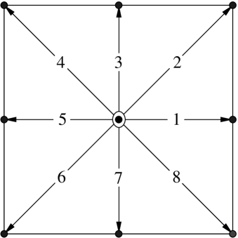
Figure 1: Nine-velocity square lattice (D2Q9).

The physical variables of water depth and velocity can be calculated as

$$h=\sum_{\alpha}f_{\alpha},$$ (9)

and

$$u_{i}=\frac{1}{h}\sum_{\alpha}e_{\alpha i}f_{\alpha}.$$ (10)

To formulate a new macroscopic lattice Boltzmann method for the shallow water equations through the macroscopic physical variables of velocity and water depth without calculating distribution functions, Eq. (7) is rewritten as

$$f_{\alpha}({\bf x},t) = f_{\alpha}({\bf x}-{\bf e}_{\alpha}\delta t,t-\delta t)-\frac{1}{\tau}[f_{\alpha}({\bf x}-{\bf e}_{\alpha}\delta t,t-\delta t)$$ (11)

$$- f_{\alpha}^{eq}({\bf x}-{\bf e}_{\alpha}\delta t,t-\delta t)]$$

$$- \frac{g\overline{h}}{e^{2}}C_{\alpha}[z_{b}({\bf x})-z_{b}({\bf x}-{\bf e}_{\alpha}\delta t)]+\frac{\delta t}{e^{2}}C_{\alpha}e_{\alpha j}F_{j}.$$

Following Zhou’s idea in MacLAB [21], setting $\tau=1$ in the above equation leads to

$$f_{\alpha}({\bf x},t) = f_{\alpha}^{eq}({\bf x}-{\bf e}_{\alpha}\delta t,t-\delta t)$$ (12)

$$- \frac{g\overline{h}}{e^{2}}C_{\alpha}[z_{b}({\bf x})-z_{b}({\bf x}-{\bf e}_{\alpha}\delta t)]+\frac{\delta t}{e^{2}}C_{\alpha}e_{\alpha j}F_{j}.$$

Taking $\sum$ Eq. (12) and $\sum e_{\alpha i}$Eq. (12) yields

$$\sum f_{\alpha}({\bf x},t) = \sum f_{\alpha}^{eq}({\bf x}-{\bf e}_{\alpha}\delta t,t-\delta t)$$ (13)

$$- \frac{g}{e^{2}}\sum C_{\alpha}\overline{h}[z_{b}({\bf x})-z_{b}({\bf x}-{\bf e}_{\alpha}\delta t)]+\frac{\delta t}{e^{2}}\sum C_{\alpha}e_{\alpha j}F_{j},$$

and

$$\sum e_{\alpha i}f_{\alpha}({\bf x},t) = \sum e_{\alpha i}f_{\alpha}^{eq}({\bf x}-{\bf e}_{\alpha}\delta t,t-\delta t)+\frac{\delta t}{e^{2}}\sum C_{\alpha}e_{\alpha i}e_{\alpha j}F_{j}$$ (14)

$$- \frac{g}{e^{2}}\sum C_{\alpha}e_{\alpha i}\overline{h}[z_{b}({\bf x})-z_{b}({\bf x}-{\bf e}_{\alpha}\delta t)].$$

As $\sum f_{\alpha}({\bf x},t)=h({\bf x},t)$ and $\sum e_{\alpha i}f_{\alpha}({\bf x},t)=h({\bf x},t)u_{i}({\bf x},t)$ due to the requirement for the conservation of mass and momentum in the lattice Botlzmann dynamics, the above two equations become

$$h({\bf x},t) = \sum f_{\alpha}^{eq}({\bf x}-{\bf e}_{\alpha}\delta t,t-\delta t)$$ (15)

$$- \frac{g}{e^{2}}\sum C_{\alpha}\overline{h}[z_{b}({\bf x})-z_{b}({\bf x}-{\bf e}_{\alpha}\delta t)]+\frac{\delta t}{e^{2}}\sum C_{\alpha}e_{\alpha j}F_{j}$$

and

$$h({\bf x},t)u_{i}({\bf x},t) = \sum e_{\alpha i}f_{\alpha}^{eq}({\bf x}-{\bf e}_{\alpha}\delta t,t-\delta t)+\frac{\delta t}{e^{2}}\sum C_{\alpha}e_{\alpha i}e_{\alpha j}F_{j}$$ (16)

$$- \frac{g}{e^{2}}\sum C_{\alpha}e_{\alpha i}\overline{h}[z_{b}({\bf x})-z_{b}({\bf x}-{\bf e}_{\alpha}\delta t)].$$

According to the centred scheme [7, 23] the force term $F_{j}$ can be evaluated at the midpoint between $({\bf x}-{\bf e}_{\alpha}\delta t,t-\delta t)$ and $({\bf x},t)$ as

$$F_{j}=F_{j}\left({\bf x}-\frac{1}{2}{\bf e}_{\alpha}\delta t,t-\frac{1}{2}\delta t\right).$$ (17)

It can be seen from Eqs. (15) and (16) that the water depth and velocity can be determined using the macroscopic physical variables through the local equilibrium distribution function without calculating the distribution function from Eq. (7) that is required in Eqs. (9) and (10) for determination of the depth and velocity. These equations form the macroscopic lattice Boltzmann method for shallow water equations (MacLABSWE). It shows through the recovery procedure in Appendix that the eddy viscosity $\nu$ in the absence of collision step can be naturally taken into account using the particle speed $e$ from

$$e=6{\nu}/{\delta x},$$ (18)

instead of $e=\delta x/\delta t$ to calculate the local equilibrium distribution function $f_{\alpha}^{eq}$ from Eq. (8). Apparently, after a lattice size $\delta x$ is chosen, the model is ready to simulate a flow with an eddy viscosity $\nu$ because $(x_{j}-e_{\alpha j}\delta t)$ stands for a neighbouring lattice point; $f_{\alpha}^{eq}$ at time of $(t-\delta t)$ represents its known quantity at the current time; and the particle speed $e$ is determined from Eq. (18) for use in computation of $f_{\alpha}^{eq}$. In addition, the time step $\delta t$ is no longer an independent parameter but is calculated as $\delta t=\delta x/e$, which is used in simulations of unsteady flows. Consequently, only the lattice size $\delta x$ is required in the MacLABSWE for simulation of shallow water flows, bringing the eLABSWE into a precise “Lattice” Boltzmann method for shallow water flows. This enables the model to become an automatic simulator without tuning other simulation parameters, making it possible and easy to model a large flow system when a super-fast computer such as a quantum computer becomes available in the future.

The method is unconditionally stable as it shares the same valid condition as that for $f_{\alpha}^{eq}$, or the Mack number $M=U_{c}/e$ is much smaller than 1, in which $U_{c}$ is a characteristic flow speed. The Mack number can also be expressed as a lattice Reynolds number of $R_{le}=U_{c}\delta x/\nu$ via Eq. (18). In practical simulations, it is found that the model is stable if $R_{le}=U_{m}\delta x/\nu<1$ where $U_{m}$ is the maximum flow speed and is used as the characteristic flow speed. The main features of the MacLABSWE are that there is no collision operator and only macroscopic physical variables such as depth and velocity are required, which are directly retained as boundary conditions with a minimum memory requirement. At the same time, the most efficeint bounce-back scheme can be implemented as that in the standard lattice Botlzmann method if it is required, e.g., if the water depth is unknown and no-slip boundary condition is applied at south boundary for a straight channel, $f_{2}^{eq},\ f_{3}^{eq},\ f_{4}^{eq}$ in Eq. (15) are unknown and they can be determined as $f_{2}^{eq}=f_{6}^{eq},\ f_{3}^{eq}=f_{7}^{eq},\ f_{4}^{eq}=f_{8}^{eq}$ using the bounce-back scheme, after which the water depth can be determined from Eq. (15) and in this case Eq. (16) is no longer required for calculation of velocity as the initial zero velocity will retain as no-slip boundary condition there. The simulation procedure for MacLABSWE is

1. Initialise water depth and velocity,

2. Choose the lattice size $\delta x$ and determine the particle speed $e$ from Eq. (18),

3. Calculate $f_{\alpha}^{eq}$ from Eq. (8) using depth and velocity,

4. Update the depth and velocity using Eqs. (15) and (16),

5. Apply the boundary conditions if necessary, and repeat Step b until a solution is reached.

The only limitation of the described model is that, for small eddy viscosity or high speed flow, the chosen lattice size after satisfying $R_{le}<1$ may turn out to generate very large lattice points (Lattice points, e.g., for one dimension with length of $L$ is calculated as $N_{L}=L/\delta x$ and $N_{L}$ is the lattice points); if the total lattice points is too big such that the demanding computations is beyond the current power of a computer, the simulation cannot be carried out. Such difficulties may be solved or relaxed through parallel computing using computer techniques such as GPU processors and multiple servers, and will largely or completely removed using quantum computing when a quantum computer becomes available.

4 Validation

In order to verify the described model, three numerical tests are presented. The SI Units are used for the physical variables in the following numerical simulations.

4.1 1D tidal flow

First of all, a tidal flow over an irregular bed is predicted, which is a common flow problem in coastal engineering. The bed is defined with data listed in Table 1.

Table 1: Bed elevation $z_{b}$ for irregular bed.

$x(m)$	0	50	100	150	250	300	350	400	425	435
$z_{b}(m)$	0	0	2.5	5	5	3	5	5	7.5	8
$x(m)$	450	475	500	505	530	550	565	575	600	650
$z_{b}(m)$	9	9	9.1	9	9	6	5.5	5.5	5	4
$x(m)$	700	750	800	820	900	950	1000	1500
$z_{b}(m)$	3	3	2.3	2	1.2	0.4	0	0

Here we consider a 1D problem with the initial and boundary conditions of

$$h(x,0)=16-z_{b}(x),$$ (19)

$$u_{x}(x,0)=0$$ (20)

and

$$h(0,t)=20-4\sin\left[\pi\left(\frac{4t}{86,400}+\frac{1}{2}\right)\right],$$ (21)

$$u_{x}(1500,t)=0.$$ (22)

In the simulation, $\delta x=7.5\ m$ or $200$ lattices are used with eddy viscosity of $\nu=31.25\ m^{2}/s$ for same computational parameters used in [15]. This is an unsteady flow. Two numerical results at $t=10,800\ s$ and $t=32,400\ s$ corresponding to the half-risen tidal flow with maximum positive velocities and to the half-ebb tidal flow with maximum negative velocities are compared with the analytical solutions [24] and depicted in Figs. 2 and 3, respectively. The maximum relative errors are less than 0.005% for the water level, less than 0.05% for velocity larger than 0.002 $m/s$, and less than 0.3% for smaller velocity, revealing excellent agreements.

Figure 2: Comparison of velocity at $t=10,800\ s$ when flow is in the half-risen tide with maximum positive velocities for 1D tidal flow.

Figure 3: Comparison of velocity at $t=32,400\ s$ when the flow is in the half-ebb tide with maximum negative velocities for 1D tidal flow.

4.2 2D wind-driven circulation

Secondly, we consider a wind-driven circulation in a lake, which may generate a complex flow phenomenon depending on the bed topography of a lake. In this test, a uniform wind shear stress is applied to the shallow water in a circular basin with the bed topography defined by the still water depth $H$,

$$H(x,y)=\frac{1}{1.3}\left(\frac{1}{2}+\sqrt{\frac{1}{2}-\frac{\sqrt{x^{2}+y^{2}}}{386.4}}\right),$$ (23)

from which, the bed level can be determined as $z_{b}(x,y)=H(0,0)-H(x,y)$. The same dish-shaped basin is also used by Rogers et al. [25] to test a Godunov-type method. Initially, the water in the basin is still and then a uniform wind speed of $u_{w}=5\ m/s$ blows from southwest to northeast, at which wind shear stress is calculated from Eq. (4). Its steady flow consists of two relatively strong counter-rotating gyres with flow in the deeper water against the direction of the wind, exhibiting complex flow phenomenon. In the numerical computation, $\delta x=2$ or $200\times 200$ lattices are used with eddy viscosity of $\nu=5.33\ m^{2}/s$. After the steady solution is obtained, the flow field is shown in Fig. 4 and the normalised resultant velocities at cross section $A-A$ are compared with the analytical solution [26] in Fig. 5, exhibiting similar agreement to that by Zhou [16] for the same test. Although there is discrepancy between the numerical prediction and the analytical solution, such agreement is reasonable due to the fact that the assumptions of both the rigid-lid approximation for the water surface and a parabolic distribution for the eddy viscosity were used in deriving the analytical solution.

Figure 4: Flow field for wind-driven flow, showing well-developed counter-rotating gyres with flow in the deeper water against the direction of the wind.

Figure 5: Comparison of the resultant velocities along Cross-section A-A (see Fig. 4) with the analytical solution [26], where $U_{0}=0.129$ and $\ s=u_{x}+u_{y}$.

4.3 Flow over a 2D hump

Finally, a steady shallow water flow over a 2D hump is investigated. The 2D hump is defined as

$$z_{b}(x,y)=\left\{\begin{array}[]{lr}\psi(x,y),&\mbox{if }(x,y)\in\Omega,\\ 0,&\mbox{otherwise},\end{array}\right.$$ (24)

where $\Omega=[300,500]\times[400,600]$ and

$$\psi(x,y)=\sin^{2}\left(\frac{\pi(x-300)}{200}\right)\sin^{2}\left(\frac{\pi(y-400)}{200}\right).$$ (25)

The flow conditions are: discharge per unit width is $q=10\ m^{2}/s$; water depth is $h=10\ m$ at the outflow boundary and the channel is $1000\ m$ long and $1000\ m$ wide. This is the same test as that used by researchers in validation of numerical methods [27, 28, 29] for sediment transport under shallow water flows. Here only steady flow over the fixed bed without sediment transport is simulated as prediction of correct flow plays an essential role in determination of bed evolution, and hence it is a suitable test for the proposed scheme. We use $\delta x=5$ or $200\times 200$ lattices in the simulation. After the steady solution is obtained, the velocities $u_{x}$ and $u_{y}$ are shown in Figs. 6 and 7, respectively, demonstrating good agreements with those obtained using high-resolution Godunov-type numerical methods [27, 28, 29].

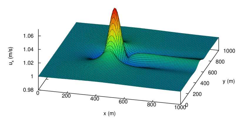
Figure 6: Velocity $u_{x}$ distribution for a steady flow over a 2D bump.

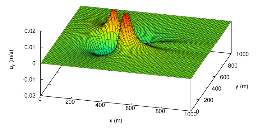
Figure 7: Velocity $u_{y}$ distribution for a steady flow over a 2D bump.

5 Conclusions

The paper presents a novel macroscopic lattice Boltzmann method for shallow water equations (MacLABSWE). Only streaming step is required in the model. This changes the stardard view of two integral steps of streaming and collision in the lattice Boltzmann method. The method is unconditionally stable. The physical variables can be directly applied as boundary condition without coverting them to their corresponding distribution functions. This greatly simplifies the procedure and needs less storage of computer. The MacLABSWE preserves the simple arithmetic calculations of the lattice Boltzmann method at the full advantages of the lattice Boltzann method. The most efficient bounce-back scheme can be applied straightforward if it is required. Steady and unsteady numerical tests have shown that the method can provide accurate solutions, making the MacLABSWE an ideal model for simulating shallow water flows.

Appendix: Recovery of shallow water equations

As the MacLABSWE is the special case where $\tau=1$ in Eq. (11), without loss of generality, we can show how to recover the shallow water eqautions (1) and (2) from it. For this we take a Taylor expansion to the terms on the right-hand side of Eq. (11), $f_{\alpha}({\bf x}-{\bf e}_{\alpha}\delta t,t-\delta t)$ and $f_{\alpha}^{eq}({\bf x}-{\bf e}_{\alpha}\delta t,t-\delta t)$, in time and space at point $({\bf x},t)$, and have

$$f_{\alpha}({\bf x}-{\bf e}_{\alpha}\delta t,t-\delta t) = f_{\alpha}-\delta t\left(\frac{\partial}{\partial t}+e_{\alpha j}\frac{\partial}{\partial x_{j}}\right)f_{\alpha}$$ (26)

$$+ \frac{1}{2}\delta t^{2}\left(\frac{\partial}{\partial t}+e_{\alpha j}\frac{\partial}{\partial x_{j}}\right)^{2}f_{\alpha}+{\cal O}(\delta t^{3})$$

and

$$f_{\alpha}^{eq}({\bf x}-{\bf e}_{\alpha}\delta t,t-\delta t) = f_{\alpha}^{eq}-\delta t\left(\frac{\partial}{\partial t}+e_{\alpha j}\frac{\partial}{\partial x_{j}}\right)f_{\alpha}^{eq}$$ (27)

$$+ \frac{1}{2}\delta t^{2}\left(\frac{\partial}{\partial t}+e_{\alpha j}\frac{\partial}{\partial x_{j}}\right)^{2}f_{\alpha}^{eq}+{\cal O}(\delta t^{3}).$$

According to the Chapman-Enskog analysis, $f_{\alpha}$ can be expanded in a series of $\delta t$,

$$f_{\alpha}=f_{\alpha}^{(0)}+\delta tf_{\alpha}^{(1)}+\delta t^{2}f_{\alpha}^{(2)}+{\cal O}(\delta t^{3}).$$ (28)

Eq. (17) can be written, via a Taylor expansion, as

$$F_{j}\left({\bf x}-\frac{1}{2}{\bf e}_{\alpha}\delta t,t-\frac{1}{2}\delta t\right)=F_{j}-\frac{\delta t}{2}\left(\frac{\partial}{\partial t}+e_{\alpha j}\frac{\partial}{\partial x_{j}}\right)F_{j}+{\cal O}(\delta t^{2}).$$ (29)

The forth term on the right hand side of Eq. (11) can also be expressed via the Taylor expansion,

$$\frac{gC_{\alpha}}{e^{2}}\left[h-\frac{\delta t}{2}\left(\frac{\partial h}{\partial t}+e_{\alpha j}\frac{\partial h}{\partial x_{j}}\right)\right]\left(\delta te_{\alpha j}\frac{\partial z_{b}}{\partial x_{j}}-\frac{\delta t^{2}}{2}e_{\alpha i}e_{\alpha j}\frac{\partial^{2}z_{b}}{\partial x_{i}\partial x_{j}}\right)+{\cal O}(\delta t^{3}).$$ (30)

After substitution of Eqs. (26) - (30) into Eq. (11), we have the expressions to order $\delta t^{0}$

$$f_{\alpha}^{(0)}=f_{\alpha}^{eq},$$ (31)

to order $\delta t$

$$\left(\frac{\partial}{\partial t}+e_{\alpha j}\frac{\partial}{\partial x_{j}}\right)f_{\alpha}^{(0)}=-\frac{f_{\alpha}^{(1)}}{\tau}-\frac{ghC_{\alpha}e_{\alpha j}}{e^{2}}\frac{\partial z_{b}}{\partial x_{j}}+\frac{C_{\alpha}e_{\alpha j}F_{j}}{e^{2}},$$ (32)

and to order $\delta t^{2}$ as

$$\left(1-\frac{1}{\tau}\right)\left(\frac{\partial}{\partial t}\right.+\left.e_{\alpha j}\frac{\partial}{\partial x_{j}}\right)f_{\alpha}^{(1)}-\frac{1}{2}\left(\frac{\partial}{\partial t}+e_{\alpha j}\frac{\partial}{\partial x_{j}}\right)^{2}f_{\alpha}^{(0)}=$$

$$\hskip 36.98857pt-\frac{1}{\tau}f_{\alpha}^{(2)}+\frac{C_{\alpha}ge_{\alpha j}}{2e^{2}}\left(\frac{\partial h}{\partial t}+e_{\alpha i}\frac{\partial h}{\partial x_{i}}\right)\frac{\partial z_{b}}{\partial x_{j}}$$

$$\hskip 36.98857pt+\frac{ghC_{\alpha}e_{\alpha i}e_{\alpha j}}{2e^{2}}\frac{\partial^{2}z_{b}}{\partial x_{i}\partial x_{j}}-\frac{C_{\alpha}e_{\alpha j}}{2e^{2}}\left(\frac{\partial F_{j}}{\partial t}+e_{\alpha i}\frac{\partial F_{j}}{\partial x_{i}}\right).$$ (33)

Substitution of Eq. (32) into Eq. (33) gives

$$\left(1-\frac{1}{2\tau}\right)\left(\frac{\partial}{\partial t}+e_{\alpha j}\frac{\partial}{\partial x_{j}}\right)f_{\alpha}^{(1)}=-\frac{1}{\tau}f_{\alpha}^{(2)}.$$ (34)

Taking $\sum$ [(32) + $\delta t\times$ (34)] about $\alpha$ provides

$$\frac{\partial}{\partial t}\sum_{\alpha}f_{\alpha}^{(0)}+\frac{\partial}{\partial x_{j}}\sum_{\alpha}e_{\alpha j}f_{\alpha}^{(0)}=0.$$ (35)

Evaluation of the terms in the above equation using Eq. (8) results in the second-order accurate continuity equation (1).

Taking $\sum$ $e_{\alpha i}$ [(32) + $\delta t\times$ (34)] about $\alpha$ yields

$$\frac{\partial}{\partial t}\sum_{\alpha}e_{\alpha i}f_{\alpha}^{(0)}+\frac{\partial}{\partial x_{j}}\sum_{\alpha}e_{\alpha i}e_{\alpha j}f_{\alpha}^{(0)}+$$

$$\hskip 17.07164pt\delta t(1-\frac{1}{2\tau})\frac{\partial}{\partial x_{j}}\sum_{\alpha}e_{\alpha i}e_{\alpha j}f_{\alpha}^{(1)}=-gh\frac{\partial z_{b}}{\partial x_{i}}+F_{i}.$$ (36)

After the terms are simplified with Eq. (8) and some algebra, the above equation becomes the momentum equation (2), which is second-order accurate, where the eddy viscosity $\nu$ is defined by

$$\nu=\frac{e^{2}\delta t}{6}(2\tau-1).$$ (37)

As the above general derivation is carried out for a constant of $\tau$, setting $\tau=1$ also recovers the shallow water equations. In this case, Eq. (37) becomes Eq. (18).

It must be pointed out that (a) the implicitness related to $\overline{h}$ can be eliminated by using the method by He et al. [30]; (b) alternatively, the following semi-implicit form,

$$\overline{h}=0.5[h({\bf x},t)+h({\bf x}-{\bf e}_{\alpha}\delta t,t)],$$ (38)

can be used, which is simple and demonstrated to produce accurate solutions, and hence it is preferred in practice.

References

- [1] C. B. Vreugdenhil. Numerical Methods for Shallow-water Flow. Kluwer Academic Publishers, Dordrecht, 1994.
- [2] A. Alcrudo and P. Garcia-Navarro. A High Resolution Godunov-Type Scheme in Finite Volumes for the 2D Shallow Water Equations. International Journal for Numerical Methods in Fluids, 16:489–505, 1993.
- [3] V. Casulli. “Semi-implicit Finite Difference Methods for the Two-dimensional Shallow Water Equations”. J. Comput. Phys., 86:56–74, 1990.
- [4] A. G. L. Borthwick and G. A. Akponasa. “Reservoir flow prediction by contravariant shallow water equations”. J. Hydr. Eng. Div., ASCE, 123(5):432–439, 1997.
- [5] B. Yulistiyanto, Y. Zech, and W. H. Graf. Flow around a cylinder: shallow-water modeling with diffusion-dispersion. Journal of Hydraulic Engineering, ASCE, 124(4):419–429, 1998.
- [6] K. Hu, C. G. Mingham, and D. M. Causon. Numerical simulation of wave overtopping of coastal structures using the non-linear shallow water equations. Coastal Engineering, 41(4):433–465, 2000.
- [7] J. G. Zhou. Lattice Boltzmann Methods for Shallow Water Flows. Springer-Verlag, Berlin, 2004.
- [8] J. G. Zhou. Velocity-depth coupling in shallow water flows. J. Hydr. Eng., ASCE, 121(10):717–724, 1995.
- [9] J. G. Zhou, D. M. Causon, C. G. Mingham, and D. M. Ingram. The surface gradient method for the treatment of source terms in the shallow-water equations. Journal of Computational Physics, 168:1–25, 2001.
- [10] J. G. Zhou. A lattice Boltzmann model for the shallow water equations. Computer methods in Applied Mechanics and Engineering, 191(32):3527–3539, 2002.
- [11] M. R. Swift, W. R. Osborn, and J. M. Yeomans. Lattice Boltzmann simulation of nonideal fluids. Physical Review Letters, 75:830–833, 1995.
- [12] M. A. A. Spaid and F. R. Phelan, Jr. Lattice boltzmann method for modeling microscale flow in fibrous porous media. Phys. Fluids, 9(9):2468–2474, 1997.
- [13] J. G. Zhou. A lattice Boltzmann model for groundwater flows. International Journal of Modern Physics C, 18:973–991, 2007.
- [14] J. G. Zhou. Lattice Boltzmann morphodynamic model. Journal of Computational Physics, 270:255–264, 2014.
- [15] J. G. Zhou. Enhancement of the LABSWE for shallow water flows. Journal of Computational Physics, 230:394–401, 2011.
- [16] J. G. Zhou and H. Liu. Determination of bed elevation in the enhanced lattice Boltzmann method for the shallow-water equations. Physical Review E, 88:023302, 2013.
- [17] H. Liu, J. G. Zhou, and R. Burrows. Lattice boltzmann model for shallow water flows in curved and meandering channels. International Journal of Computational Fluid Dynamics, 23:209–220, 2009.
- [18] H. Liu, J. G. Zhou, and R. Burrows. Multi-block lattice boltzmann simulations of subcritical flow in open channel junctions. Computers and Fluids, 38:1108–1117, 2009.
- [19] H. Liu, J. G. Zhou, and R. Burrows. Numerical modelling of turbulent compound channel flow using the lattice boltzmann method. International Journal for Numerical Methods in Fluids, 59:753–765, 2009.
- [20] H. Liu, J. G. Zhou, M. Li, and Y. Zhao. Multi-block lattice Boltzmann simulations of solute transport in shallow water flows. Advances in Water Resources, 58:24–40, 2013.
- [21] J. G. Zhou. Macroscopic lattice boltzmann method. arXiv:1901.02716, 2019.
- [22] P. L. Bhatnagar, E. P. Gross, and M. Krook. A model for collision processes in gases. I: small amplitude processes in charged and neutral one-component system. Physical Review, 94(3):511–525, 1954.
- [23] J. G. Zhou. Axisymmetric lattice Boltzmann method revised. Phys. Rev. E, 84:036704, 2011.
- [24] A. Bermudez and M. E. Vázquez. Upwind methods for hyperbolic conservation laws with source terms. Computers and Fluids, 23:1049–1071, 1994.
- [25] B. Rogers, M. Fujihara, and A. G. L. Borthwick. Adaptive Q-tree Godunov-type scheme for shallow water equations. International Journal for Numerical Methods in Fluids, 35:247–280, 2001.
- [26] C. Kranenburg. Wind-driven chaotic advection in a shallow model lake. J. Hydr. Res., 30(1):29–46, 1992.
- [27] J. Hudson and P. K. Sweby. A high-resolution scheme for the equations governing 2d bed-load sediment transport. International Journal for Numerical Methods in Fluids, 47(10-11):1085–1091, 2005.
- [28] J. Huang, A. G. L. Borthwick, and R. L. Soulsby. Adaptive quadtree simulation of sediment transport. Proceedings of Institution of Civil Engineers: Journal of Engineering and Computational Mechanics, 163(EM2):101–110, 2010.
- [29] Fayssal Benkhaldoun, Slah Sahmim, and Mohammed Seaïd. A two-dimensional finite volume morphodynamic model on unstructured triangular grids. International Journal for Numerical Methods in Fluids, 63:1296–1327, 2010.
- [30] X. He, S. Chen, and G. D. Doolen. A novel thermal model for the lattice boltzmann method in incompressible limit. Journal of Computational Physics, 146:282–300, 1998.