New insight into results of Ostrowski and Lang
on sums of remainders using Farey sequences

Abstract.

The sums $S(x,t)$ of the centered remainders $kt-\lfloor kt\rfloor-1/2$ over $k\leq x$ and corresponding Dirichlet series were studied by A. Ostrowski, E. Hecke, H. Behnke and S. Lang for fixed real irrational numbers $t$. Their work was originally inspired by Weyl’s equidistribution results modulo 1 for sequences in number theory.

In a series of former papers we obtained limit functions which describe scaling properties of the Farey sequence of order $n$ for $n\to\infty$ in the vicinity of any fixed fraction $a/b$ and which are independent of $a/b$. We extend this theory on the sums $S(x,t)$ and also obtain a scaling behaviour with a new limit function. This method leads to a refinement of results given by Ostrowski and Lang and establishes a new proof for the analytic continuation of related Dirichlet series. We will also present explicit relations to the theory of Farey sequences.

1. Introduction

In [17] Hermann Weyl developed a general and far-reaching theory for the equidistribution of sequences modulo 1, which is discussed from a historical point of view in Stammbach’s paper [16]. Especially Weyl’s result that for real $t$ the sequence $t,\,2t,\,3t,\,\ldots$ is equidistributed modulo 1 if and only if $t$ is irrational can be found in [17, §1]. This means that

$$\lim\limits_{N\to\infty}\frac{1}{N}\#\left\{nt-\lfloor nt\rfloor\in[a,b]:n\leq N\right\}=b-a$$

holds for all subintervals $[a,b]\subseteq[0,1]$ if and only if $t\in\mathbb{R}\setminus\mathbb{Q}$. Here $\#M$ denotes the number of elements of a finite set $M$. This generalization of Kronecker’s Theorem [4, Chapter XXIII, Theorem 438] is an important result in number theory. We have only mentioned its one dimensional version, but the higher dimensional case is also treated in Weyl’s paper.

Now we put

(1.1) $$S(x,t)=\sum\limits_{k\leq x}\left(kt-\lfloor kt\rfloor-\frac{1}{2}\right)$$

for $x\geq 0$ and $t\in\mathbb{R}$. If the sequence $(nt)_{n\in\mathbb{N}}$ is “well distributed” modulo 1 for irrational $t$, then $|S(x,t)|/x$ should be “small” for $x$ large enough.

In [14, Equation (2), p. 80] Ostrowski used the continued fraction expansion $t=\langle\lambda_{0},\lambda_{1},\lambda_{2},\ldots\rangle$ for irrational $t$ and presented a very efficient calculation of $S(n,t)$ with $n\in\mathbb{N}_{0}$. He namely obtained a simple iterative procedure using at most $\mathcal{O}(\log n)$ steps for $n\to\infty$, uniformly in $t\in\mathbb{R}$. We have summarized his result in Theorem 2.5 of the paper on hand. From this theorem he derived an estimate for $S(n,t)$ in the case of irrational $t\in\mathbb{R}$ which depends on the choice of $t$. Especially if $(\lambda_{k})_{k\in\mathbb{N}_{0}}$ is a bounded sequence, then we say that $t$ has bounded partial quotients, and have in this case from Ostrowski’s paper

(1.2) $$|S(n,t)|\leq C(t)\log n\,,\quad n\geq 2\,,$$

with a constant $C(t)>0$ depending on $t$ . Ostrowski also showed that this gives the best possible result, answering an open question posed by Hardy and Littlewood.

In [11] and [12, III,§1] Lang obtained for every fixed $\varepsilon>0$ that

(1.3) $$|S(n,t)|\leq\left(\log n\right)^{2+\varepsilon}\quad\mbox{~{}for ~{}}n\geq n_{0}(t,\varepsilon)$$

for almost all $t\in\mathbb{R}$ with a constant $n_{0}(t,\varepsilon)\in\mathbb{N}$. Let $\alpha$ be an irrational real number and $g\geq 1$ be an increasing function, defined for sufficiently large positive numbers. Due to Lang [12, II,§1] the number $\alpha$ is of type $\leq g$ if for all sufficiently large numbers $B$, there exists a solution in relatively prime integers $q,p$ of the inequalities

$$|q\alpha-p|<1/q\,,\quad B/g(B)\leq q<B\,.$$

After Corollary 2 in [12, II,§3], where Lang studied the quantitative connection between Weyl’s equidistribution modulo 1 for the sequence $t,2t,3t,\ldots$ and the type of the irrational number $t$, he mentioned the work of Ostrowski [14] and Behnke [1] and wrote: ”Instead of working with the type as we have defined it, however, these last-mentioned authors worked with a less efficient way of determining the approximation behaviour of $\alpha$ with respect to $p/q$, whence followed weaker results and more complicated proofs.”

Though Lang’s theory gives Ostrowski’s estimate (1.2) for all real irrational numbers $t$ with bounded partial quotients, see [12, II, §2, Theorem 6 and III,§1, Theorem 1], as well as estimate (1.3) for almost all $t\in\mathbb{R}$, Lang did not use Ostrowski’s efficient formula for the calculation of $S(n,t)$ . We will see in Section 3 of the paper on hand that Ostrowski’s formula can be used as well in order to derive estimate (1.3) for almost all $t\in\mathbb{R}$, without working with the type defined in [12, II,§1]. For this purpose we will present the general and useful Theorem 2.6, which will be derived in Section 2 from the elementary theory of continued fractions. Our resulting new Theorems 3.5, 3.3 now have the advantage to provide an explicit form for those sets of $t$-values which satisfy crucial estimates of $S(n,t)$.
If $\Theta:[1,\infty)\to[1,\infty)$ is any monotonically increasing function with $\displaystyle\lim\limits_{n\to\infty}\Theta(n)=\infty$ , then Theorem 3.3 gives the inequality $|S(n,t)|\leq 2\log^{2}(n)\Theta(n)$ uniformly for all $n\geq 3$ and all $t\in\mathcal{M}_{n}$ for a sequence of sets $\mathcal{M}_{n}\subseteq[0,1]$ with $\lim\limits_{n\to\infty}|\mathcal{M}_{n}|=1$. Here $|\mathcal{M}_{n}|$ denotes the Lebesgue-measure of $\mathcal{M}_{n}$. On the other hand Theorem 2.3 states that

$$\left(\int\limits_{0}^{1}S(n,t)^{2}\,dt\right)^{1/2}=\mathcal{O}(\sqrt{n})\quad\text{for~{}}n\to\infty$$

gives the true order of magnitude for the $L_{2}(0,1)$-norm of $S(n,\cdot)$. If $\Theta$ increases slowly then the values of $S(n,t)$ with $t$ in the unit-interval $[0,1]$ which give the major contribution to the $L_{2}(0,1)$-norm have their pre-images only in the small complements $[0,1]\setminus\mathcal{M}_{n}$. We see that $n_{0}(t,\varepsilon)$ in estimate (1.3) depends substantially on the choice of $t$. Moreover, a new representation formula for $B_{n}(t)=S(n,t)/n$ given in Section 2, Theorem 2.2 will also give an alternative proof of Ostrowski’s estimate (1.2) if $t$ has bounded partial quotients. In this way we summarize and refine the corresponding results given by Ostrowski and Lang, respectively.

For $n\in\mathbb{N}$ and $N=\sum\limits_{k=1}^{n}\varphi(k)$ with Euler’s totient function $\varphi$ the Farey sequence $\mathcal{F}_{n}$ of order $n$ consists of all reduced and ordered fractions

$$\frac{0}{1}=\frac{a_{0,n}}{b_{0,n}}<\frac{a_{1,n}}{b_{1,n}}<\frac{a_{2,n}}{b_{2,n}}<\ldots<\frac{a_{N,n}}{b_{N,n}}=\frac{1}{1}$$

with $1\leq b_{\alpha,n}\leq n$ for $\alpha=0,1,\ldots,N$. By $\mathcal{F}^{ext}_{n}$ we denote the extension of $\mathcal{F}_{n}$ consisting of all reduced and ordered fractions $\frac{a}{b}$ with $a\in\mathbb{Z}$ and $b\in\mathbb{N}$, $b\leq n$.

In the former paper [9] we have studied 1-periodic functions $\Phi_{n}:\mathbb{R}\to\mathbb{R}$ which are related to the Farey sequence $\mathcal{F}_{n}$, based on the theory developed in [6, 7, 8] for related functions. For $k\in\mathbb{N}$ and $x>0$ we use the Möbius function $\mu$ and define the 1-periodic functions $q_{k},\Phi_{x}:\mathbb{R}\to\mathbb{R}$ given by

(1.4) $$\begin{split}q_{k}(t)&=-\sum\limits_{d|k}\mu(d)\,\beta\left(\frac{kt}{d}\right)~{}\,\mbox{with}~{}\,\beta(t)=t-\lfloor t\rfloor-\frac{1}{2}\,,\\ \Phi_{x}\left(t\right)&=\frac{1}{x}\sum\limits_{k\leq x}q_{k}(t)=-\frac{1}{x}\sum\limits_{j\leq x}\sum\limits_{k\leq x/j}\mu(k)\beta\left(jt\right)\,.\\ \end{split}$$

The functions $\Phi_{x}$ determine the number of Farey fractions in prescribed intervals. More precisely, $t\sum\limits_{k\leq n}\varphi(k)+n\Phi_{n}(t)+\frac{1}{2}$ gives the number of fractions of $\mathcal{F}^{ext}_{n}$ in the interval $[0,t]$ for $t\geq 0$ and $n\in\mathbb{N}$. Moreover, there is a connection between the functions $S(x,t)$ and $\Phi_{x}(t)$ via the Mellin-transform and the Riemann-zeta function, namely the relation

$$\int\limits_{1}^{\infty}\frac{S(x,t)}{x^{s+1}}dx=-\zeta(s)\,\int\limits_{1}^{\infty}\frac{\Phi_{x}(t)}{x^{s}}dx\,,$$

valid for $\Re(s)>1$ and any fixed $t\in\mathbb{R}$. We will use it in a modified form in Theorem 3.7.

In contrast to Ostrowski’s approach using elementary evaluations of $S(n,t)$ for real values of $t$, Hecke [5] considered the case of special quadratic irrational numbers $t$, studied the analytical properties of the corresponding Dirichlet series

(1.5) $$\sum\limits_{m=1}^{\infty}\frac{mt-\lfloor mt\rfloor-\frac{1}{2}}{m^{s}}=s\int\limits_{1}^{\infty}\frac{S(x,t)}{x^{s+1}}dx$$

and obtained its meromorphic continuation to the whole complex plane, including the location of poles. Hecke could use his analytical method to derive estimates for $S(n,t)$, but he did not obtain Ostrowski’s optimal result (1.2) for real irrationalities $t$ with bounded partial quotients.

For positive irrational numbers $t$ Sourmelidis [15] studied analytical relations between the Dirichlet series in (1.5) and the so called Beatty zeta-functions and Sturmian Dirichlet series.

For $x>0$ we set

$$r_{x}=\frac{1}{x}\sum\limits_{k\leq x}\varphi(k)\,,\quad s_{x}=\sum\limits_{k\leq x}\frac{\varphi(k)}{k}\,,$$

and define the continuous and odd function $h:\mathbb{R}\to\mathbb{R}$ by

$$h(x)=\begin{cases}0&\ \text{for}\ x=0\,,\\ 3x/\pi^{2}+r_{x}-s_{x}&\ \text{for}\ x>0\,,\\ -h(-x)&\ \text{for}\ x<0\,.\\ \end{cases}$$

Then we obtained in [9, Theorem 2.2] for any fixed reduced fraction $a/b$ with $a\in\mathbb{Z}$ and $b\in\mathbb{N}$ and any $x_{*}>0$ that for $n\to\infty$

$$\tilde{h}_{a,b}(n,x)=-b\,\Phi_{n}\left(\frac{a}{b}+\frac{x}{bn}\right)$$

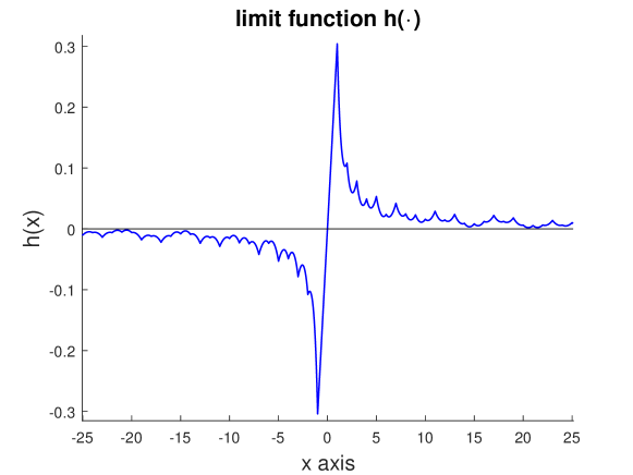
Figure 1. Plot of $h(x)$ for $-25\leq x\leq 25$ .

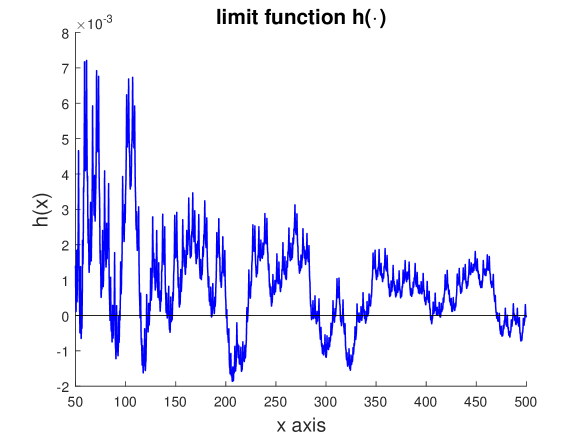
Figure 3. Plot of $h(x)$ for $50\leq x\leq 500$ .

converges uniformly to $h(x)$ for $-x_{*}\leq x\leq x_{*}$. For this reason we have called $h$ a limit function. It follows from [13, Theorem 1] with an absolute constant $c>0$ for $x\geq 2$ that $\displaystyle h(x)=\mathcal{O}\left(e^{-c\sqrt{\log x}}\right)\,.$ Plots of this limit function are presented in Section 4, Figures 1,2,3.

In Section 2 we introduce another limit function ${\tilde{\eta}}:\mathbb{R}\to\mathbb{R}$ defined by ${\tilde{\eta}}(0)=-\frac{1}{2}$ and

$${\tilde{\eta}}(x)=\frac{(x-\lfloor x\rfloor)(x-\lfloor x\rfloor-1)}{2x}\quad\text{for}\ x\in\mathbb{R}\setminus\{0\}\,,$$

and obtain from Theorem 3.2 for $B_{n}(t)=S(n,t)/n$ analogous to [9, Theorem 2.2] the new result that for $n\to\infty$

$$\tilde{\eta}_{a,b}(n,x)=b\,B_{n}\left(\frac{a}{b}+\frac{x}{bn}\right)$$

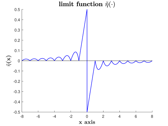
Figure 4. Plot of $\tilde{\eta}(x)$ for $-8\leq x\leq 8$ .

converges uniformly to $\tilde{\eta}(x)$ for $-x_{*}\leq x\leq x_{*}$. A plot of ${\tilde{\eta}}(x)$ for $-8\leq x\leq 8$ is given in Section 4, Figure 4. Now Theorem 2.2(b) follows from part (a) and leads to the formula (2.18), which bears a strong resemblance to that in Ostrowski’s Theorem 2.5 and gives an alternative proof for Ostrowski’s estimate (1.2) if $t$ has bounded partial quotients. Hence it would be interesting to know whether there is a deeper reason for this analogy.

2. Sums with sawtooth functions

With the sawtooth function $\beta(t)=t-\lfloor t\rfloor-\frac{1}{2}$ we define for $x>0$ the 1-periodic functions $B_{x}:\mathbb{R}\to\mathbb{R}$ by

(2.1) $$B_{x}\left(t\right)=\frac{1}{x}\sum\limits_{k\leq x}\beta(kt)\,.$$

Next we will state [8, Theorem 2.2] which, amongst other things, connects the study of the functions $B_{x}$ with the theory of Farey fractions.

Theorem 2.1.

[8, Theorem 2.2] Assume that $\frac{a}{b}<\frac{a^{*}}{b^{*}}$ are consecutive reduced fractions in the extended Farey sequence $\mathcal{F}^{ext}_{b}$ of order $b\leq n$ with $b,b^{*},n\in\mathbb{N}$. For $q\geq 0$ we define

(2.2) $$\xi_{+}(q)=\frac{a^{*}+aq}{b^{*}+bq}\,,\qquad x_{+}(q)=\frac{n}{b^{*}+bq}\,,$$

and see that its inverse functions

$$\xi_{+}^{-1}(\xi)=\frac{a^{*}-b^{*}\xi}{b\xi-a}\,,\qquad x_{+}^{-1}(x)=\frac{n/x-b^{*}}{b}\,$$

are defined for $a/b<\xi\leq a^{*}/b^{*}$ and $0<x\leq n/b^{*}$, respectively.

• We assume that

  $$\frac{a}{b}<\frac{A}{B}\leq\frac{a^{*}}{b^{*}}$$

  with the reduced fraction $\xi=\frac{A}{B}\in\mathcal{F}^{ext}_{n}$, $A\in\mathbb{Z}$, $B\in\mathbb{N}$, and put

  $$q=\frac{Ba^{*}-Ab^{*}}{Ab-Ba}\,,\qquad\alpha=\left\lfloor x_{+}(q)\right\rfloor\,.$$

  Then $\alpha,Ab-Ba\in\mathbb{N}$, and $q$ is reduced with $q=\xi_{+}^{-1}(\xi)\in\mathcal{F}^{ext}_{\alpha}\,.$

• Let $0\leq q=\frac{a^{\prime}}{b^{\prime}}$ be reduced, assume that $\alpha=\left\lfloor x_{+}(q)\right\rfloor\geq 1$ and that $q\in\mathcal{F}^{ext}_{\alpha}$. We put

  $$\xi=\frac{a^{*}b^{\prime}+aa^{\prime}}{b^{*}b^{\prime}+ba^{\prime}}\,.$$

  Then $\xi$ is a reduced fraction of $\mathcal{F}^{ext}_{n}$ in the interval $(a/b,a^{*}/b^{*}]$ satisfying $\xi=\xi_{+}(q)$ .

The function $\beta(t)$ has jumps of height $-1$ exactly at integer numbers $t\in\mathbb{Z}$ but is continuous elsewhere. Let $a/b$ with $a\in\mathbb{Z}$, $b\in\mathbb{N}$ be any reduced fraction with denominator $b\leq x$.

By $\displaystyle u^{\pm}(t)=\lim\limits_{\varepsilon\downarrow 0}u(t\pm\varepsilon)$ we denote the one-handed limits of a real- or complex valued function $u$ with respect to the real variable $t$.

Then the height of the jump of $B_{x}$ at $a/b$ is given by

(2.3) $$B_{x}^{+}(a/b)-B_{x}^{-}(a/b)=-\frac{1}{x}\left\lfloor\frac{x}{b}\right\rfloor\,.$$

We introduce the function ${\tilde{\eta}}:\mathbb{R}\to\mathbb{R}$ given by ${\tilde{\eta}}(0)=-\frac{1}{2}$ and

(2.4) $${\tilde{\eta}}(x)=\frac{(x-\lfloor x\rfloor)(x-\lfloor x\rfloor-1)}{2x}\quad\text{for}\ x\in\mathbb{R}\setminus\{0\}\,.$$

The function ${\tilde{\eta}}$ is continuous apart from the zero-point with derivative

(2.5) $${\tilde{\eta}}^{\prime}(x)=\frac{1}{2}-\frac{\lfloor x\rfloor(\lfloor x\rfloor+1)}{2x^{2}}\quad\text{for}~{}x\in\mathbb{R}\setminus\mathbb{Z}\,.$$

In the following theorem we assume that $\frac{a}{b}<\frac{a^{*}}{b^{*}}$ are consecutive reduced fractions in the extended Farey sequence $\mathcal{F}^{ext}_{b}$ of order $b\leq n$ with $b,b^{*},n\in\mathbb{N}$.

Theorem 2.2.

• For $0<x\leq n/b^{*}$ we have

  $$\begin{split}&B_{n}\left(\frac{a}{b}+\frac{x}{bn}\right)=B_{n}\left(\frac{a}{b}\right)+\frac{1}{2b}+\frac{{\tilde{\eta}}(x)}{b}-\frac{x}{n}\,B_{x}^{-}\left(\frac{n/x-b^{*}}{b}\right)\\ &+\frac{x}{2bn}+\frac{1}{n}\,\sum\limits_{k\leq x}\beta\left(\frac{n-kb^{*}}{b}\right)\,.\\ \end{split}$$

• For $0<t\leq 1$ and $n\in\mathbb{N}$ we have

  $$B_{n}\left(t\right)={\tilde{\eta}}(tn)-\frac{\lfloor tn\rfloor}{n}\,B_{\lfloor tn\rfloor}^{-}\left(\frac{1}{t}-\left\lfloor\frac{1}{t}\right\rfloor\right)+\frac{tn-\lfloor tn\rfloor}{2n}\,.$$

Proof.

Since (b) follows from (a) in the special case $a=0$, $a^{*}=b^{*}=b=1$, it is sufficient to prove (a). We define for $0<x\leq n/b^{*}$:

(2.6) $$\begin{split}R_{n}\left(\frac{a}{b},x\right)&=-b\left(B_{n}\left(\frac{a}{b}+\frac{x}{bn}\right)-B_{n}\left(\frac{a}{b}\right)\right)\\ &+\frac{1}{2}+{\tilde{\eta}}(x)-\frac{bx}{n}\,B_{x}^{-}\left(\frac{n/x-b^{*}}{b}\right)+\frac{x}{2n}\,.\\ \end{split}$$

We use (2.1), (2.5) and obtain, except of the discrete set of jump discontinuities of $R_{n}$, its derivative

$$\begin{split}\frac{d}{dx}R_{n}\left(\frac{a}{b},x\right)&=-b\cdot\frac{n+1}{2}\cdot\frac{1}{bn}+\frac{1}{2}-\frac{\lfloor x\rfloor(\lfloor x\rfloor+1)}{2x^{2}}\\ &-\frac{b}{n}\,\frac{d}{dx}\left(x\,B_{x}^{-}\left(\frac{n/x-b^{*}}{b}\right)\right)+\frac{1}{2n}\\ &=-\frac{\lfloor x\rfloor(\lfloor x\rfloor+1)}{2x^{2}}-\frac{b}{n}\,\frac{d}{dx}\sum\limits_{k\leq\lfloor x\rfloor}\beta^{-}\left(k\,\frac{n/x-b^{*}}{b}\right)\\ &=-\frac{\lfloor x\rfloor(\lfloor x\rfloor+1)}{2x^{2}}-\frac{b}{n}\sum\limits_{k\leq\lfloor x\rfloor}k\cdot\frac{n}{b}\cdot\left(-\frac{1}{x^{2}}\right)=0\,.\\ \end{split}$$

Note that $B_{n}=B_{n}^{+}$ and $R_{n}=R^{+}_{n}$. We deduce from Theorem 2.1 for any $x$ in the interval $0<x\leq n/b^{*}$ that $\displaystyle a/b+x/(bn)$ is a jump discontinuity of $B_{n}$ if and only if $\displaystyle(n/x-b^{*})/b$ is a jump discontinuity of $B_{x}$. Let $x_{+}(q)$ be defined by the second equation in (2.2) and let

$$q=\frac{a^{\prime}}{b^{\prime}}=\frac{n/x_{+}(q)-b^{*}}{b}$$

be any reduced fraction $a^{\prime}/b^{\prime}\in\mathcal{F}^{ext}_{\lfloor x_{+}(q)\rfloor}$ from Theorem 2.1(b). We use (2.3) and have

(2.7) $$-b(B_{n}^{+}-B_{n}^{-})\left(\frac{a}{b}+\frac{x_{+}(q)}{nb}\right)=\frac{b}{n}\left\lfloor\frac{n}{b^{*}b^{\prime}+ba^{\prime}}\right\rfloor=\frac{b}{n}\left\lfloor\frac{x_{+}(q)}{b^{\prime}}\right\rfloor\,.$$

First we consider the case that $x_{+}(q)$ is a non-integer number. Using again (2.3) we obtain

(2.8) $$\begin{split}&\lim\limits_{x\,\downarrow\,x_{+}(q)}\left(x\,B_{x}^{-}\left(\frac{n/x-b^{*}}{b}\right)\right)-\lim\limits_{x\,\uparrow\,x_{+}(q)}\left(x\,B_{x}^{-}\left(\frac{n/x-b^{*}}{b}\right)\right)\\ &=x_{+}(q)\cdot\left(B_{x_{+}(q)}^{-}-B_{x_{+}(q)}^{+}\right)\left(\frac{a^{\prime}}{b^{\prime}}\right)=\left\lfloor\frac{x_{+}(q)}{b^{\prime}}\right\rfloor\,,\end{split}$$

taking into account that $(n/x-b^{*})/b$ is monotonically decreasing with respect to $x$. For (2.7) and (2.8) we note that $a^{*}b-ab^{*}=1$ for the Farey fractions $a/b<a^{*}/b^{*}$ in Theorem 2.1 and recall that $B_{n}$ has a jump at

$$\frac{a}{b}+\frac{x_{+}(q)}{nb}=\frac{a(b^{*}+bq)+a^{*}b-ab^{*}}{b(b^{*}+bq)}=\frac{a^{*}b^{\prime}+aa^{\prime}}{b^{*}b^{\prime}+ba^{\prime}}=\xi_{+}(q)$$

if and only if $B_{x_{+}(q)}$ has a jump at $q=a^{\prime}/b^{\prime}$. We obtain from (2.6), (2.7), (2.8) that

$$\left(R_{n}^{+}-R_{n}^{-}\right)\left(\frac{a}{b},x_{+}(q)\right)=\frac{b}{n}\left\lfloor\frac{x_{+}(q)}{b^{\prime}}\right\rfloor-\frac{b}{n}\left\lfloor\frac{x_{+}(q)}{b^{\prime}}\right\rfloor=0\,.$$

This implies that $R_{n}$ is free from jumps at non-integer arguments $x$. It remains to calculate the jumps of $R_{n}$ at any integer argument $k$ with $0<k\leq n/b^{*}$. Here we also have to take care of the jump in $B_{x}=B_{k}$ with respect to the index $x=k$, and conclude

(2.9) $$\begin{split}&\lim\limits_{x\,\downarrow\,k}\left(x\,B_{x}^{-}\left(\frac{n/x-b^{*}}{b}\right)\right)-\lim\limits_{x\,\uparrow\,k}\left(x\,B_{x}^{-}\left(\frac{n/x-b^{*}}{b}\right)\right)\\ &=\lim\limits_{\varepsilon\,\downarrow\,0}\left[\sum\limits_{j\leq k}\beta^{-}\left(j\cdot\frac{\frac{n}{k+\varepsilon}-b^{*}}{b}\right)-\sum\limits_{j<k}\beta^{-}\left(j\cdot\frac{\frac{n}{k-\varepsilon}-b^{*}}{b}\right)\right]\\ &=\sum\limits_{j\leq k}\beta^{-}\left(j\cdot\frac{n/k-b^{*}}{b}\right)-\sum\limits_{j\leq k}\beta^{+}\left(j\cdot\frac{n/k-b^{*}}{b}\right)+\beta\left(\frac{n-kb^{*}}{b}\right)\\ &=\beta\left(\frac{n-kb^{*}}{b}\right)-k\left(B_{k}^{+}-B_{k}^{-}\right)\left(\frac{n/k-b^{*}}{b}\right)\,.\end{split}$$

Using (2.6), (2.9) we obtain

$$\begin{split}\left(R_{n}^{+}-R_{n}^{-}\right)\left(\frac{a}{b},k\right)&=-\frac{b}{n}\,\beta\left(\frac{n-kb^{*}}{b}\right)\\ &-b\,(B_{n}^{+}-B_{n}^{-})\left(\frac{a}{b}+\frac{k}{bn}\right)\\ &+\frac{b}{n}k\,(B_{k}^{+}-B_{k}^{-})\left(\frac{n/k-b^{*}}{b}\right)\,.\\ \end{split}$$

Due to (2.7) and Theorem 2.1 the second and third terms on the right-hand side cancel each other.

We conclude that $R_{n}$ is a step function with respect to $x$ for a given fraction $a/b$ which has jumps of height

$$R_{n}^{+}\left(\frac{a}{b},k\right)-R_{n}^{-}\left(\frac{a}{b},k\right)=-\frac{b}{n}\,\beta\left(\frac{n-kb^{*}}{b}\right)$$

only at integer numbers $k$ with $0<k\leq n/b^{*}$. To complete the proof of the theorem we only have to note that $\displaystyle\lim\limits_{\varepsilon\,\downarrow\,0}R_{n}(a/b,\varepsilon)=0\,.$ ∎

Franel [3] and Landau [10] made use of the identity

(2.10) $$\int\limits_{0}^{1}\beta(mx)\beta(nx)dx=\frac{(m,n)^{2}}{12mn}\,,$$

which is valid for all $m,n\in\mathbb{N}$. A proof of this identity can be found in [10, page 203] as well as in Edward’s textbook [2, Section 12.2]. We need it for the following

Theorem 2.3.

For $x\to\infty$ we have with the $L_{2}(0,1)$-Norm $\|\cdot\|_{2}$

$$\|B_{x}\|_{2}=\mathcal{O}\left(\frac{1}{\sqrt{x}}\right)\,.$$

On the other hand we have a constant $C>0$ with

$$\|B_{x}\|_{2}\geq\frac{C}{\sqrt{x}}\quad\text{for~{}}x\geq 1\,.$$

Proof.

We obtain from (2.10)

$$\begin{split}\|B_{x}\|_{2}^{2}&=\frac{1}{12x^{2}}\sum\limits_{m,n\leq x}\frac{(m,n)^{2}}{mn}=\frac{1}{12x^{2}}\sum\limits_{d\leq x}\sum\limits_{\underset{(m,n)=d}{m,n\leq x\,:}}\frac{d^{2}}{mn}\\ &=\frac{1}{12x^{2}}\sum\limits_{d\leq x}\sum\limits_{\underset{(j,k)=1}{j,k\leq x/d\,:}}\frac{1}{jk}\leq\frac{1}{12x^{2}}\sum\limits_{d\leq x}\sum\limits_{j,k\leq x/d}\frac{1}{jk}\\ &\leq\frac{1}{12x^{2}}\sum\limits_{d\leq x}\left(\log(x/d)+2\right)^{2}=\mathcal{O}\left(\frac{1}{x}\right)\quad\text{for}~{}x\to\infty\\ \end{split}$$

with Euler’s summation formula, regarding that

$$\int\limits_{1}^{x}\left(\log(x/t)+2\right)^{2}\,dt=10(x-1)-6\log(x)-\log(x)^{2}=\mathcal{O}\left(x\right)\,,\quad x\geq 1\,.$$

To complete the proof we note that

$$\|B_{x}\|_{2}^{2}=\frac{1}{12x^{2}}\sum\limits_{d\leq x}\sum\limits_{\underset{(j,k)=1}{j,k\leq x/d\,:}}\frac{1}{jk}\geq\frac{1}{12x^{2}}\sum\limits_{d\leq x}1=\frac{\lfloor x\rfloor}{12x^{2}}\,.$$

∎

The next two theorems employ the elementary theory of continued fractions. We will use them to derive estimates for $B_{n}(t)$ with $t$ in certain subsets $\mathcal{M}_{n},\tilde{\mathcal{M}}_{n}\subset(0,1)$ and $\lim\limits_{n\to\infty}|\mathcal{M}_{n}|=\lim\limits_{n\to\infty}|\tilde{\mathcal{M}}_{n}|=1$.

First we recall some basic facts and notations about continued fractions. For $\lambda_{0}\in\mathbb{R}$ and $\lambda_{1},\lambda_{2},\ldots,\lambda_{m}>0$ the finite continued fraction $\langle\lambda_{0},\lambda_{1},\ldots,\lambda_{m}\rangle$ is defined recursively by $\langle\lambda_{0}\rangle=\lambda_{0}$, $\langle\lambda_{0},\lambda_{1}\rangle=\lambda_{0}+1/\lambda_{1}$ and

$$\langle\lambda_{0},\lambda_{1},\ldots,\lambda_{m}\rangle=\langle\lambda_{0},\ldots,\lambda_{m-2},\lambda_{m-1}+1/\lambda_{m}\rangle\,,\quad m\geq 2\,.$$

Moreover, if $\lambda_{j}\geq 1$ is given for all $j\in\mathbb{N}$, then the limit

$$\lim\limits_{m\to\infty}\langle\lambda_{0},\lambda_{1},\ldots,\lambda_{m}\rangle=\langle\lambda_{0},\lambda_{1},\lambda_{2}\ldots\rangle$$

exists and defines an infinite continued fraction. Especially for integer numbers $\lambda_{0}\in\mathbb{Z}$ and $\lambda_{1},\lambda_{2},\ldots\in\mathbb{N}$ we obtain a unique representation

$$t=\langle\lambda_{0},\lambda_{1},\lambda_{2}\ldots\rangle$$

for all $t\in\mathbb{R}\setminus\mathbb{Q}$ in terms of an infinite continued fraction. For the determination of the coefficients $\lambda_{j}$ we need the following

Definition 2.4.

For given $t\in\mathbb{R}\setminus\mathbb{Q}$ we define a sequence of irrational numbers by

$$\vartheta_{0}=t\,,\quad\vartheta_{j}=\frac{1}{\vartheta_{j-1}-\lfloor\vartheta_{j-1}\rfloor}>1\,,\quad j\in\mathbb{N}\,.$$

We may also write $\vartheta_{j}=\vartheta_{j}(t)$ in order to indicate that the quantities $\vartheta_{j}$ depend on the fixed number $t$.

We have

(2.11) $$\lambda_{0}=\lfloor t\rfloor\,,~{}\lambda_{j}=\lfloor\vartheta_{j}(t)\rfloor\quad\text{and~{}}t=\langle\lambda_{0},\ldots,\lambda_{j-1},\vartheta_{j}(t)\rangle\quad\text{for ~{} all ~{}}j\in\mathbb{N}\,.$$

The following theorem is due to A. Ostrowski. It allows a very efficient calculation of the values $B_{n}(t)$ in terms of the continued fraction expansion of $t$.

Theorem 2.5.

Ostrowski [14, Equation (2), p. 80]
Put $S(n,t)=\sum\limits_{k\leq n}\beta(kt)=nB_{n}(t)$ for $n\in\mathbb{N}_{0}$ and $t\in\mathbb{R}$. Given are the continued fraction expansion $t=\langle\lambda_{0},\lambda_{1},\lambda_{2},\ldots\rangle$ of any fixed $t\in\mathbb{R}\setminus\mathbb{Q}$ and $n\in\mathbb{N}$. Then there is exactly one index $j_{*}\in\mathbb{N}$ with $b_{j_{*}}\leq n<b_{j_{*}+1}$, where $\displaystyle a_{k}/b_{k}=\langle\lambda_{0},\ldots,\lambda_{k-1}\rangle$ are reduced fractions $a_{k}/b_{k}$ and $k,b_{k}\in\mathbb{N}$. Put

$$n^{\prime}=n-b_{j_{*}}\left\lfloor\frac{n}{b_{j_{*}}}\right\rfloor\,.$$

Then we have

(2.12) $$S(n,t)=S(n^{\prime},t)+\frac{(-1)^{j_{*}}}{2}\left\lfloor\frac{n}{b_{j_{*}}}\right\rfloor\left(1-\rho_{j_{*}}(n+n^{\prime}+1)\right)$$

with $\rho_{j_{*}}=|b_{j_{*}}t-a_{j_{*}}|$ and

(2.13) $$\left\lfloor\frac{n}{b_{j_{*}}}\right\rfloor\leq\lambda_{j_{*}}\,,\quad 0<\left|1-\rho_{j_{*}}(n+n^{\prime}+1)\right|<1\,.$$

Following Ostrowski’s strategy we note two important conclusions. We fix any number $t=\langle\lambda_{0},\lambda_{1},\lambda_{2},\ldots\rangle\in\mathbb{R}\setminus\mathbb{Q}$ and apply Ostrowski’s Theorem 2.5 successively, starting with the calculation of $S(n,t)$ and $\displaystyle|S(n,t)|\leq|S(n^{\prime},t)|+\lambda_{j_{*}}/2$ . If $n^{\prime}=0$, then $S(n^{\prime},t)=0$, and we are done. Otherwise we replace $n$ by the reduced number $n^{\prime}$ with $0<n^{\prime}<b_{j_{*}}$ and apply Ostrowski’s Theorem again, and so on. For the final calculation of $S(n,t)$ we need at most ${j_{*}}$ applications of the recursion formula and conclude from (2.12), (2.13) that

(2.14) $$n|B_{n}(t)|=|S(n,t)|\leq\frac{1}{2}\,\sum\limits_{k=1}^{j_{*}}\lambda_{k}\,.$$

From $b_{0}=0$, $b_{1}=1$ and $b_{j+1}=b_{j-1}+\lambda_{j}b_{j}$ for $j\in\mathbb{N}$ we obtain $b_{j+1}\geq 2b_{j-1}$, and hence for all $j\geq 3$ that $\displaystyle b_{j}\geq 2^{\frac{j-1}{2}}\,.$ Since $n\geq b_{j_{*}}$, we obtain without restrictions on $j_{*}$ for $n\geq 3$ that $\displaystyle n\geq 2^{\frac{j_{*}-1}{2}}$ and

(2.15) $$\begin{split}j_{*}\leq 1+\frac{2}{\log 2}\log n\leq\left(1+\frac{2}{2/3}\right)\log n=4\log n\,,\quad n\geq 3\,.\end{split}$$

We will see that (2.14) and (2.15) have important conclusions. An immediate consequence is Ostrowski’s estimate (1.2) for irrational numbers $t$ with bounded partial quotients, but first shed new light on these estimates by using Theorem 2.2(b) instead of Theorem 2.5. We put $J_{*}=(0,1)\setminus\mathbb{Q}$ and fix any $t\in J_{*}$ and $n\in\mathbb{N}$. The sequence

(2.16) $$t_{0}=t\,,\quad t_{j}=\frac{1}{t_{j-1}}-\left\lfloor\frac{1}{t_{j-1}}\right\rfloor$$

with $j\in\mathbb{N}$ is infinite, whereas the corresponding sequence of non-negative integer numbers

$$n_{0}=n\,,\quad n_{j}=\lfloor t_{j-1}n_{j-1}\rfloor$$

is strictly decreasing and terminates if $n_{j}=0$. Therefore $n_{j^{\prime}}=0$ for some index $j^{\prime}\in\mathbb{N}$. We assume $1\leq j<j^{\prime}$ and distinguish the two cases $0<t_{j-1}<1/2$ and $1/2<t_{j-1}<1$. In the first case we have $n_{j+1}<n_{j}<n_{j-1}/2$, and in the second case again

$$n_{j+1}=\lfloor t_{j}\lfloor t_{j-1}n_{j-1}\rfloor\rfloor<t_{j}t_{j-1}n_{j-1}=(1-t_{j-1})n_{j-1}<n_{j-1}/2\,.$$

If $j^{\prime}$ is odd, then

$$n=n_{0}\geq 2^{\frac{j^{\prime}-1}{2}}n_{j^{\prime}-1}\geq 2^{\frac{j^{\prime}-1}{2}}\,,$$

otherwise

$$n=n_{0}\geq n_{1}\geq 2^{\frac{j^{\prime}-2}{2}}n_{j^{\prime}-1}\geq 2^{\frac{j^{\prime}-2}{2}}\,,$$

and $n\geq 2^{\frac{j^{\prime}-2}{2}}$ in both cases. Therefore

(2.17) $$j^{\prime}\leq 2+\frac{2}{\log 2}\log n\leq\left(1+\frac{2}{\log 2}\right)\log n\leq 4\log n\,,\quad n\geq 8\,.$$

Estimate (2.17) bears a strong resemblance with (2.15). Now it follows from Theorem 2.2(b) that

(2.18) $$B_{n}(t)=\sum\limits_{j=0}^{j^{\prime}-1}(-1)^{j}\left(\frac{n_{j}}{n}{\tilde{\eta}}(t_{j}n_{j})+\frac{t_{j}n_{j}-\lfloor t_{j}n_{j}\rfloor}{2n}\right)\,.$$

For the sequence in (2.16) we have $\vartheta_{j+1}t_{j}=1$ for all $j\in\mathbb{N}_{0}$, and we obtain from the definition (2.4) of ${\tilde{\eta}}$ that

$$\frac{n_{j}}{n}{\tilde{\eta}}(t_{j}n_{j})+\frac{t_{j}n_{j}-\lfloor t_{j}n_{j}\rfloor}{2n}=-\frac{t_{j}n_{j}-\lfloor t_{j}n_{j}\rfloor}{2n}\left(\vartheta_{j+1}\left(1-\left(t_{j}n_{j}-\lfloor t_{j}n_{j}\rfloor\right)\right)-1\right)\,.$$

Here $\vartheta_{j+1}>1$ implies $|\vartheta_{j+1}\left(1-\left(t_{j}n_{j}-\lfloor t_{j}n_{j}\rfloor\right)\right)-1|\leq\max(1,\vartheta_{j+1}-1)$. We see from (2.18) with Definition 2.4 and (2.11) that

(2.19) $$\left|B_{n}(t)\right|\leq\sum\limits_{j=0}^{j^{\prime}-1}\frac{\max(1,\vartheta_{j+1}-1)}{2n}\leq\frac{1}{2n}\sum\limits_{k=1}^{j^{\prime}}\lambda_{k}\,.$$

The calculations of $B_{n}(t)$ with Ostrowski’s Theorem 2.5 on one hand and with (2.18) on the other hand are similar but different. Especially $j_{*}$ in Theorem 2.5 and $j^{\prime}$ used in (2.18) are different in general. If we use (2.15) and (2.17) then estimates (2.19) and (2.14) both give the same result. Hence Theorem 2.2(b) may be used as well instead of Ostrowski’s Theorem for an efficient calculation and estimation of $B_{n}(t)$ and $S(n,t)$. This is a surprising analogy.

Theorem 2.6.

Given are integer numbers $\alpha_{1},\ldots,\alpha_{m}\in\mathbb{N}$. We put $J_{*}=(0,1)\setminus\mathbb{Q}$. Using Definition 2.4 with the functions $\vartheta_{j}$ depending on $t\in J_{*}$ we obtain for the measure $|\mathcal{M}|$ of the set

$$\mathcal{M}=\left\{t\in J_{*}\,:\,\vartheta_{j}(t)<\alpha_{j}\quad\text{for~{}all~{}}j=1,\ldots,m\right\}$$

the estimates

$$\prod\limits_{j=1}^{m}\left(1-\frac{1}{\alpha_{j}}\right)^{2}\leq|\mathcal{M}|\leq\prod\limits_{j=1}^{m}\left(1-\frac{1}{\alpha_{j}}\right)\,.$$

Proof.

The desired result is valid for $m=1$ with $\displaystyle\mathcal{M}=\left\{t\in J_{*}\,:\,1/t<\alpha_{1}\right\}$ and $\displaystyle|\mathcal{M}|=1-1/\alpha_{1}\,.$ Assume that the statement of the theorem is already true for a given $m\in\mathbb{N}$. We prescribe $\alpha_{m+1}\in\mathbb{N}$ and will use induction to prove the statement for $m+1$.

For all $j\in\mathbb{N}$ and general given numbers $\lambda_{0}\in\mathbb{R}$ and $\lambda_{1},\ldots,\lambda_{j-1}>0$ we put for $1\leq k<j$:

(2.20) $$\begin{split}a_{0}=1\,,~{}a_{1}=\lambda_{0}\,,~{}&a_{k+1}=a_{k-1}+\lambda_{k}a_{k}\,,\\ b_{0}=0\,,~{}b_{1}=1\,,~{}&b_{k+1}=b_{k-1}+\lambda_{k}b_{k}\,.\\ \end{split}$$

We have

(2.21) $$\begin{split}&\langle\lambda_{0},\lambda_{1},\ldots\lambda_{j-1},x\rangle-\langle\lambda_{0},\lambda_{1},\ldots\lambda_{j-1},x^{\prime}\rangle\\ &=\frac{(-1)^{j}(x-x^{\prime})}{(b_{j}x+b_{j-1})(b_{j}x^{\prime}+b_{j-1})}\quad\text{for ~{}}x,x^{\prime}>0\,.\end{split}$$

Especially for $\lambda_{0}=0$ and integer numbers $\lambda_{1},\ldots,\lambda_{j}\in\mathbb{N}$ we define the set $J(\lambda_{1},\ldots,\lambda_{j})$ consisting of all $t\in J_{*}$ between the two rational numbers $\langle 0,\lambda_{1},\ldots,\lambda_{j-1},\lambda_{j}\rangle$ and $\langle 0,\lambda_{1},\ldots,\lambda_{j-1},\lambda_{j}+1\rangle$.

It follows from (2.20),(2.21) and all $j\in\mathbb{N}$ that

(2.22) $$|J(\lambda_{1},\ldots,\lambda_{j})|=\frac{1}{(b_{j}(\lambda_{j}+1)+b_{j-1})(b_{j}\lambda_{j}+b_{j-1})}\,.$$

The sets $J(k)=(1/(k+1),1/k)\setminus\mathbb{Q}$ with $k\in\mathbb{N}$ form a partition of $J_{*}=(0,1)\setminus\mathbb{Q}$. More general, it follows from Definition 2.4 and (2.11) for fixed numbers $\lambda_{1},\ldots,\lambda_{j}\in\mathbb{N}$ that the pairwise disjoint sets $J(\lambda_{1},\ldots,\lambda_{j},k)$ with $k\in\mathbb{N}$ form a partition of the set $J(\lambda_{1},\ldots,\lambda_{j})$. We conclude by induction with respect to $j$ that the pairwise disjoint sets $J(\lambda_{1},\ldots,\lambda_{j})$ with $(\lambda_{1},\ldots,\lambda_{j})\in\mathbb{N}^{j}$ also form a partition of $J_{*}$.

Now we put $j=m$ and distinguish two cases, $m$ odd and $m$ even, respectively. In both cases, $m$ odd or $m$ even, the union

$$\bigcup\limits_{k=1}^{\alpha_{m+1}-1}J(\lambda_{1},\ldots,\lambda_{m},k)$$

is the set of all numbers $t\in J_{*}$ with $\lfloor\vartheta_{j}(t)\rfloor=\lambda_{j}$ for $j=1,\ldots,m$ such that $\vartheta_{m+1}(t)<\alpha_{m+1}$. We define the set

$$\mathcal{M}^{\prime}=\left\{t\in J_{*}\,:\,\vartheta_{j}(t)<\alpha_{j}\quad\text{for~{}all~{}}j=1,\ldots,m+1\right\}$$

and conclude

(2.23) $$|\mathcal{M}^{\prime}|=\sum\limits_{\lambda_{1}=1}^{\alpha_{1}-1}\sum\limits_{\lambda_{2}=1}^{\alpha_{2}-1}\cdots\sum\limits_{\lambda_{m}=1}^{\alpha_{m}-1}\sum\limits_{k=1}^{\alpha_{m+1}-1}|J(\lambda_{1},\ldots,\lambda_{m},k)|\,.$$

It also follows from our induction hypothesis that

(2.24) $$\begin{split}&\prod\limits_{j=1}^{m}\left(1-\frac{1}{\alpha_{j}}\right)^{2}\\ \leq&\sum\limits_{\lambda_{1}=1}^{\alpha_{1}-1}\sum\limits_{\lambda_{2}=1}^{\alpha_{2}-1}\cdots\sum\limits_{\lambda_{m}=1}^{\alpha_{m}-1}|J(\lambda_{1},\ldots,\lambda_{m})|\leq\prod\limits_{j=1}^{m}\left(1-\frac{1}{\alpha_{j}}\right)\,.\\ \end{split}$$

We evaluate the inner sum in (2.23), and obtain for odd values of $m$ the telescopic sum

$$\begin{split}&\sum\limits_{k=1}^{\alpha_{m+1}-1}|J(\lambda_{1},\ldots,\lambda_{m},k)|\\ &=\sum\limits_{k=1}^{\alpha_{m+1}-1}\left(\langle 0,\lambda_{1},\ldots,\lambda_{m},k+1\rangle-\langle 0,\lambda_{1},\ldots,\lambda_{m},k\rangle\right)\\ &=\langle 0,\lambda_{1},\ldots,\lambda_{m},\alpha_{m+1}\rangle-\langle 0,\lambda_{1},\ldots,\lambda_{m},1\rangle\\ &=\langle 0,\lambda_{1},\ldots,\lambda_{m-1},\lambda_{m}+1/\alpha_{m+1}\rangle-\langle 0,\lambda_{1},\ldots,\lambda_{m-1},\lambda_{m}+1\rangle\,.\\ \end{split}$$

Apart from a minus sign on the right hand side we get the same result for even values of $m$, and hence from (2.21) with $j=m$ in both cases

(2.25) $$\begin{split}&\sum\limits_{k=1}^{\alpha_{m+1}-1}|J(\lambda_{1},\ldots,\lambda_{m},k)|\\ &=\frac{1-\frac{1}{\alpha_{m+1}}}{(b_{m}(\lambda_{m}+1)+b_{m-1})(b_{m}(\lambda_{m}+\frac{1}{\alpha_{m+1}})+b_{m-1})}\,.\\ \end{split}$$

Using $\lambda_{m}\geq 1$ we have

$$\frac{\left(1-\frac{1}{\alpha_{m+1}}\right)^{2}}{b_{m}\lambda_{m}+b_{m-1}}\leq\frac{1-\frac{1}{\alpha_{m+1}}}{b_{m}(\lambda_{m}+\frac{1}{\alpha_{m+1}})+b_{m-1}}\leq\frac{1-\frac{1}{\alpha_{m+1}}}{b_{m}\lambda_{m}+b_{m-1}}\,,$$

and obtain from (2.25) and (2.22) with $j=m$ that

(2.26) $$\begin{split}&|J(\lambda_{1},\ldots,\lambda_{m})|\left(1-\frac{1}{\alpha_{m+1}}\right)^{2}\\ &\leq\sum\limits_{k=1}^{\alpha_{m+1}-1}|J(\lambda_{1},\ldots,\lambda_{m},k)|\leq|J(\lambda_{1},\ldots,\lambda_{m})|\left(1-\frac{1}{\alpha_{m+1}}\right)\,.\\ \end{split}$$

The theorem follows from (2.23), (2.24) and (2.26). ∎

Remark 2.7.

Since $\alpha_{j}\in\mathbb{N}$ for $j\leq m$, the conditions $\vartheta_{j}(t)<\alpha_{j}$ in the definition of the set $\mathcal{M}$ may likewise be replaced by the equivalent conditions $\lambda_{j}\leq\alpha_{j}-1$, where $\lambda_{j}$ are the coefficients in the continued fraction expansion of $t$, see Definition 2.4 and (2.11) .

3. Dirichlet series related to Farey sequences

We define the sawtooth function $\beta_{0}:\mathbb{R}\to\mathbb{R}$ by

$$\beta_{0}(x)=\begin{cases}x-\lfloor x\rfloor-\frac{1}{2}&\ \text{for}\ x\in\mathbb{R}\setminus{\mathbb{Z}}\,,\\ 0&\ \text{for}\ x\in\mathbb{Z}\,.\\ \end{cases}$$

With $x>0$ the 1-periodic function $B_{x,0}:\mathbb{R}\to\mathbb{R}$ is the arithmetic mean of $B_{x}^{-}$, $B_{x}^{+}=B_{x}$, see (2.1), hence

(3.1) $$B_{x,0}\left(t\right)=\frac{1}{x}\sum\limits_{k\leq x}\beta_{0}(kt)=\frac{1}{2}\left(B_{x}^{-}(t)+B_{x}^{+}(t)\right)\,.$$

Lemma 3.1.

For (relatively prime) numbers $a\in\mathbb{Z}$ and $b\in\mathbb{N}$ we have

$$|B_{x,0}(a/b)|\leq\frac{b}{x}$$

for all $x>0$.

Proof.

Without loss of generality we may assume that $a\in\mathbb{Z}$ and $b\in\mathbb{N}$ are relatively prime. Then Lemma 2.1 in [7] states that

(3.2) $$\sum\limits_{m=1}^{b}\left\lfloor\frac{am}{b}\right\rfloor=a\frac{b+1}{2}-\frac{b-1}{2}\,.$$

We can also assume that $b\geq 2$, since $B_{x,0}(0)=0$. For $m\in\mathbb{N}$ we define the $b$-periodic sequence

$$t_{a/b}(m)=1+2b\beta\left(\frac{am}{b}\right)=2am-2b\left\lfloor\frac{am}{b}\right\rfloor-b+1\,.$$

Due to (3.2) this sequence has mean value zero over one period, i.e.

$$\sum\limits_{m\leq\,b}t_{a/b}(m)=0\,.$$

We follow [7, Section 2], regard that $|\beta(t)|\leq\frac{1}{2}$ for $t\in\mathbb{R}$ and obtain

$$\begin{split}&\max\limits_{k\in\mathbb{N}}\left|\sum\limits_{m\leq k}t_{a/b}(m)\right|\\ &=\max\limits_{1\leq k\leq b}\left|\sum\limits_{m\leq k}\left(2b\beta\left(\frac{am}{b}\right)+1\right)\right|\\ &\leq\max\limits_{1\leq k\leq b}\sum\limits_{m\leq k}(b+1)=b(b+1)\,.\\ \end{split}$$

We conclude for $x>0$ that

(3.3) $$\left|\sum\limits_{m\leq x}t_{a/b}(m)\right|\leq b(b+1)\,.$$

Next we use (2.3) and obtain

$$\begin{split}B_{x,0}(a/b)&=B_{x}(a/b)+\frac{1}{2x}\left\lfloor\frac{x}{b}\right\rfloor\\ &=\frac{1}{2bx}\sum\limits_{m\leq x}\left(t_{a/b}(m)-1\right)+\frac{1}{2x}\left\lfloor\frac{x}{b}\right\rfloor\\ &=\frac{1}{2bx}\sum\limits_{m\leq x}t_{a/b}(m)+\frac{1}{2x}\left(\left\lfloor\frac{\lfloor x\rfloor}{b}\right\rfloor-\frac{\lfloor x\rfloor}{b}\right)\,.\\ \end{split}$$

Hence we see from (3.3) with $b\geq 2$ that

$$\left|B_{x,0}(a/b)\right|\leq\frac{b+1}{2x}+\frac{1}{2x}\leq\frac{b}{x}\,.$$

∎

Using Theorem 2.2(a), Lemma 3.1, (3.1), (2.3) and for $x\in\mathbb{R}$ the symmetry relationship

$$B_{n}\left(\frac{a}{b}-\frac{x}{bn}\right)=-B_{n}^{-}\left(\frac{b-a}{b}+\frac{x}{bn}\right)\,,$$

we obtain the following result, which has the counterparts [7, Theorem 3.2] and [9, Theorem 2.2] in the theory of Farey fractions:

Theorem 3.2.

Assume that $a/b\in\mathcal{F}^{ext}_{n}$ and put

$$\tilde{\eta}_{a,b}(n,x)=b\,B_{n}\left(\frac{a}{b}+\frac{x}{bn}\right)\,,\qquad x\in\mathbb{R}\,.$$

Then for $n\to\infty$ the sequence of functions $\tilde{\eta}_{a,b}(n,\cdot)$ converges uniformly on each interval $[-x_{*},x_{*}]$, $x_{*}>0$ fixed, to the limit function $\tilde{\eta}$ in (2.4).

For the following two results we apply Theorem 2.5 and recall (2.14), (2.15). Due to Theorem 3.2 the functions $B_{n}$ cannot converge uniformly to zero on any given interval. Instead we have the following

Theorem 3.3.

Let $\Theta:[1,\infty)\to[1,\infty)$ be monotonically increasing with $\displaystyle\lim\limits_{n\to\infty}\Theta(n)=\infty\,.$

We fix $n\in\mathbb{N}$, $\varepsilon>0$, put $m=\lfloor 4\log n\rfloor$, use Definition 2.4, recall $J_{*}=(0,1)\setminus\mathbb{Q}$ and define

$$\mathcal{M}_{n}=\left\{t\in J_{*}\,:\,\vartheta_{j}(t)<1+\lfloor\Theta(n)\log n\rfloor\quad\mbox{for~{}all ~{} }j=1,\ldots,m\right\}\,.$$

Then $\displaystyle\lim\limits_{n\to\infty}|\mathcal{M}_{n}|=1$ and

(3.4) $$\left|B_{n,0}(t)\right|=\left|B_{n}(t)\right|\leq 2\,\frac{\log^{2}n}{n}\,\Theta(n)$$

for all $n\geq 3$ and all $t\in\mathcal{M}_{n}$.

Proof.

We apply Ostrowski’s Theorem on any number $t\in\mathcal{M}_{n}$ with continued fraction expansion $t=\langle 0,\lambda_{1},\lambda_{2},\ldots\rangle$ and obtain $j_{*}\leq m$ from (2.15), since $j_{*}$ is an integer number. From $j_{*}\leq m$ and $t\in\mathcal{M}_{n}$ we conclude that $\lambda_{k}\leq\Theta(n)\log n$ for $k=1,\ldots,j_{*}$, and the desired inequality follows with (2.14) . The first statement follows from Theorem 2.6 via

$$\begin{split}|\mathcal{M}_{n}|&\geq\left(1-\frac{1}{1+\lfloor\Theta(n)\log n\rfloor}\right)^{2m}\\ &\geq\left(1-\frac{1}{\Theta(n)\log n}\right)^{2m}\geq\left(1-\frac{1}{\Theta(n)\log n}\right)^{8\log n}\,,\\ \end{split}$$

since the right-hand side tends to $1$ for $n\to\infty$. ∎

Remark 3.4.

The sets $\mathcal{M}_{n}$ in the previous theorem are chosen in such a way that the large values $B_{n}(t)$ from the peaks of the rescaled limit function around the rational numbers with small denominators predicted by Theorem 3.2 can only occur in the small complements $J_{*}\setminus\mathcal{M}_{n}$ of these sets. However, the quality of the estimates of the values $B_{n}(t)$ on the sets $\mathcal{M}_{n}$ depends on the different choices of the growing function $\Theta$. For example, $\Theta(n)=1+\log\left(1+\log n\right)$ gives a much smaller bound than $\Theta(n)=16\sqrt{n}/(4+\log n)^{2}$, whereas the latter choice leads to a much smaller value of $|J_{*}\setminus\mathcal{M}_{n}|=1-|\mathcal{M}_{n}|$ .

Theorem 3.5.

Let $\Theta:[1,\infty)\to[1,\infty)$ be monotonically increasing with $\displaystyle\lim\limits_{n\to\infty}\Theta(n)=\infty\,.$ We fix $n\in\mathbb{N}$, $\varepsilon>0$, use Definition 2.4, recall $J_{*}=(0,1)\setminus\mathbb{Q}$ and put

$$\tilde{\mathcal{M}_{n}}=\left\{t\in J_{*}\,:\,\vartheta_{j}(t)<1+\lfloor\Theta(n)j^{1+\varepsilon}\rfloor\quad\text{for~{}all~{}}j\in\mathbb{N}\right\}\,.$$

Then $|\tilde{\mathcal{M}}|=1$ for $\tilde{\mathcal{M}}=\bigcup\limits_{n=1}^{\infty}\tilde{\mathcal{M}_{n}}$, and for all $t\in\tilde{\mathcal{M}}$ there exists an index $n_{0}=n_{0}(t,\varepsilon)$ with

$$\left|B_{n,0}(t)\right|=\left|B_{n}(t)\right|\leq\frac{(4\log n)^{2+\varepsilon}}{2n}\,\Theta(n)\quad\mbox{for ~{} all ~{}}n\geq n_{0}\,.$$

The complement $J_{*}\setminus\tilde{\mathcal{M}}$ is an uncountable null set which is dense in the unit interval $(0,1)$.

Proof.

The function $\Theta$ is monotonically increasing, hence $\tilde{\mathcal{M}_{1}}\subseteq\tilde{\mathcal{M}_{2}}\subseteq\tilde{\mathcal{M}_{3}}\ldots\,,$ and we have

(3.5) $$|\tilde{\mathcal{M}}|=\lim\limits_{n\to\infty}|\tilde{\mathcal{M}_{n}}|\,.$$

For all $n,k\in\mathbb{N}$ we define

$$\tilde{\mathcal{M}_{n,k}}=\left\{t\in J_{*}\,:\,\vartheta_{j}(t)<1+\lfloor\Theta(n)j^{1+\varepsilon}\rfloor\quad\text{for~{}all~{}}j=1,\ldots,k\right\}\,.$$

Then $\tilde{\mathcal{M}_{n}}=\bigcap\limits_{k=1}^{\infty}\tilde{\mathcal{M}_{n,k}}$ and

(3.6) $$|\tilde{\mathcal{M}_{n}}|=\lim\limits_{k\to\infty}|\tilde{\mathcal{M}_{n,k}}|$$

from $\tilde{\mathcal{M}_{n,1}}\supseteq\tilde{\mathcal{M}_{n,2}}\supseteq\tilde{\mathcal{M}_{n,3}}\ldots\,.$ It follows from Theorem 2.6 for all $n,k\in\mathbb{N}$ that

$$|\tilde{\mathcal{M}_{n,k}}|\geq\prod\limits_{j=1}^{k}\left(1-\frac{1}{\Theta(n)j^{1+\varepsilon}}\right)^{2}\geq\prod\limits_{j=1}^{\infty}\left(1-\frac{1}{\Theta(n)j^{1+\varepsilon}}\right)^{2}\,.$$

The product on the right-hand side is independent of $k$ and converges to $1$ for $n\to\infty$, hence $|\tilde{\mathcal{M}}|=1$ from (3.5), (3.6) . Each rational number in the interval $(0,1)$ is arbitrarily close to a member of the complement $J_{*}\setminus\tilde{\mathcal{M}}$, and the complement contains all $t=\langle 0,\lambda_{1},\lambda_{2},\lambda_{3},\ldots\rangle$ for which $(\lambda_{j})_{j\in\mathbb{N}}$ increases faster then any polynomial. We conclude that $J_{*}\setminus\tilde{\mathcal{M}}$ is an uncountable null set which is dense in the unit interval $(0,1)$. Now we choose $t\in\tilde{\mathcal{M}}$ and obtain $n_{0}\in\mathbb{N}$ with $t\in\tilde{\mathcal{M}}_{n_{0}}$. Then $t\in\tilde{\mathcal{M}}_{n}$ for all $n\geq n_{0}$, and we may assume that $n_{0}\geq 3$. Note that $n_{0}$ may depend on $t$ as well as on $\varepsilon$. We have $t=\langle 0,\lambda_{1},\lambda_{2},\lambda_{3},\ldots\rangle$ and

$$\lambda_{j}\leq\Theta(n)j^{1+\varepsilon}$$

for all $n\geq n_{0}$ and all $j\in\mathbb{N}$. We finally obtain from (2.14), (2.15) that

$$n|B_{n}(t)|=|S(n,t)|\leq\frac{1}{2}\,\sum\limits_{k=1}^{j_{*}}\lambda_{k}\leq\frac{j_{*}}{2}\Theta(n)j_{*}^{1+\varepsilon}\leq\frac{1}{2}\Theta(n)(4\log n)^{2+\varepsilon}\,,\quad n\geq n_{0}\,.$$

∎

Remark 3.6.

We replace $\varepsilon$ by $\varepsilon/2$, choose $\Theta(n)=1+\log\left(1+\log n\right)$ in the previous theorem and obtain the following result of Lang, see [11] and [12, III,§1] for more details: For $\varepsilon>0$ and almost all $t\in\mathbb{R}$ we have

$$|S(n,t)|\leq\left(\log n\right)^{2+\varepsilon}\quad\mbox{~{}for ~{}}n\geq n_{0}(t,\varepsilon)$$

with a constant $n_{0}(t,\varepsilon)\in\mathbb{N}$. Here the sum $S(n,t)$ is given by (1.1) . This doesn’t contradict Theorem 2.3, because the pointwise estimates of $S(n,t)$ and $B_{n}(t)$ in Theorem 3.5 are only valid for sufficiently large values of $n\geq n_{0}(t,\varepsilon)$, depending on the choice of $t$ and $\varepsilon$.

We conclude from Theorem 3.3 that the major contribution of $\|B_{n}\|_{2}$ comes from the small complement of $\mathcal{M}_{n}$. Indeed, the crucial point in Theorem 3.3 is that it holds for all $n\geq 3$, but not so much the fact that the upper bound in estimate (3.4) is slightly better than that in Theorem 3.5.

For $k\in\mathbb{N}$ and $x>0$ the 1-periodic functions $q_{k,0},\Phi_{x,0}:\mathbb{R}\to\mathbb{R}$ corresponding to (1.4) are defined as follows:

$$q_{k,0}(t)=-\sum\limits_{d|k}\mu(d)\,\beta_{0}\left(\frac{kt}{d}\right)~{}\,,$$

$$\Phi_{x,0}\left(t\right)=\frac{1}{x}\,\sum\limits_{k\leq x}q_{k,0}(t)=-\frac{1}{x}\sum\limits_{j\leq x}\sum\limits_{k\leq x/j}\mu(k)\,\beta_{0}\left(jt\right)\,.$$

In the half-plane $H=\{s\in\mathbb{C}\,:\,\Re(s)>1\}$ the parameter-dependent Dirichlet series $F_{\beta},F_{q}:\mathbb{R}\times H\to\mathbb{C}$ are given by

$$F_{\beta}(t,s)=\sum\limits_{k=1}^{\infty}\frac{\beta_{0}(kt)}{k^{s}}\,,\quad F_{q}(t,s)=\sum\limits_{k=1}^{\infty}\frac{q_{k,0}(t)}{k^{s}}\,.$$

Now Theorem 3.5 and (1.5) immediately gives

Theorem 3.7.

For $t\in\mathbb{R}$ and $\Re(s)>1$ we have with absolutely convergent series and integrals

• $$\begin{split}\frac{1}{s}\,F_{\beta}(t,s)=\int\limits_{1}^{\infty}B_{x,0}(t)\frac{dx}{x^{s}}\,,\quad\frac{1}{s}\,F_{q}(t,s)=\int\limits_{1}^{\infty}\Phi_{x,0}(t)\frac{dx}{x^{s}}\,.\\ \end{split}$$

• $$F_{q}(t,s)=-\frac{1}{\zeta(s)}\,F_{\beta}(t,s)\,.$$

For almost all $t$ the function $F_{\beta}(t,\cdot)$ has an analytic continuation to the half-plane $\Re(s)>0$ .

4. Appendix: Plots of the limit functions $h$ and $\tilde{\eta}$

Figure 2. Plot of $h(x)$ for $25\leq x\leq 50$ .