Pages: 20
Figures: 20

Proposed Running Head: A New Meteoroid Model

Editorial correspondence to:
Dr. Valeri Dikarev
Max-Planck-Institut für Kernphysik
Postfach 103980
69029 Heidelberg
GERMANY

Please send packages to:
Dr. Valeri Dikarev
Max-Planck-Institut für Kernphysik
Saupfercheckweg 1
69117 Heidelberg
GERMANY

Phone: 49-6221-516-543
Fax: 49-6221-516-324
E-mail address: Valeri.Dikarev@mpi-hd.mpg.de

ABSTRACT

The orbital distributions of dust particles in interplanetary space are inferred from several meteoroid data sets under the constraints imposed by the orbital evolution of the particles due to the planetary gravity and Poynting-Robertson effect. Infrared observations of the zodiacal cloud by the COBE DIRBE instrument, flux measurements by the dust detectors on board Galileo and Ulysses spacecraft, and the crater size distributions on lunar rock samples retrieved by the Apollo missions are fused into a single model. Within the model, the orbital distributions are expanded into a sum of contributions due to a number of known sources, including the asteroid belt with the emphasis on the prominent families Themis, Koronis, Eos and Veritas, as well as comets on Jupiter-encountering orbits. An attempt to incorporate the meteor orbit database acquired by the AMOR radar is also discussed.

Key Words: Meteoroids; Interplanetary Dust; Orbits

1 Introduction

We construct a new meteoroid model to predict meteoroid fluxes on spacecraft, with the revision of the earlier models (Divine, 1993; Staubach, 1996; Staubach et al., 1997) being motivated by several reasons. First of all, a mistype in the computer program has been known to affect the reduction of the Harvard Radio Meteor Project (HRMP) data (Taylor, 1995). This mistype alone had tainted the previous meteoroid models, since they relied on the reduced radar meteor distributions. Moreover, Taylor and Elford (1998) pointed out that the orbital distributions restored from the HRMP survey were affected by yet another, unaccounted bias. These authors argued that many high-speed meteors remain unregistered because they ablate too high, too far from the radar, and their echoes are too weak to detect. Having corrected the mistype, Taylor and Elford reduced the HRMP data again, accounting for the newly recognized bias as well. However, their effort was undermined by missing observation logs from the HRMP, so the reduction could not be perfected. A new meteor survey was selected for incorporation in the meteoroid model, the one conducted by the AMOR radar at Christchurch, New Zealand, in the period from 1995 to 1999 (Galligan and Baggaley, 2004).

Second, several other meteoroid data sets of high quality became available for incorporation in the model. The COBE/DIRBE infrared sky maps depicted the thermal emission of interplanetary dust (IPD) as seen from Earth-bound observatory within a wide range of solar elongations, through as many as 10 different filters from 1.25 to 240$\mu$m (Kelsall et al., 1998). The dust detectors on board Galileo and Ulysses in deep space continued their operation and collected new impact events worthwhile incorporation in model as well.

Third, the expansion of computer memory allows one today to detail the meteoroid distributions at a greatly improved level using large multi-dimensional arrays. In particular, the assumption of mathematical separability of the multi-dimensional distribution in position and velocity of meteoroids into single-argument functions of orbit elements postulated in (Divine, 1993) and replicated since then, is now partially lifted off.

Fourth, this new capacity of meteoroid model software is exploited to replace the empirical separable distributions of the previous models by the theoretical non-separable distributions of meteoroids obtained via semi-analytical dynamical simulations. These theoretical distributions, constructed for a number of possible meteoroid sources, including asteroids and comets, are then summed together with the weights assigned to fit the observations.

In this paper, we concentrate on the constructed model description and demonstration of its abilities to reproduce the incorporated data sets as well as a few others, while a separate publication is under preparation to cover various model’s impications, like the relative abundances and lifetimes of meteoroids from comets, asteroids and interstellar dust in different regions of the Solar system. In particular, Sect. 2 of this paper features a new computer code that reads the multi-dimensional distributions and produces the estimates of number densities, fluxes and velocities of so distributed particles. In Sect. 3, the dynamics of meteoroids of different sizes and origins are revisited, semi-analytical models of their steady-state distributions in orbit elements and mass are proposed. Meteoroid data sets that are incorporated in the new model are discussed in Sect. 4. The fitting of the simulated distributions to the data is described and commented in Sect. 5. The last Sect. 6 summarizes the results of modeling efforts.

2 A new computer code for meteoroid models

First applied in the engineering model by Divine (1993), the concept of phase density of meteoroids is at the core of the new model, too. The number of particles of reference mass per unit coordinate space and velocity space volumes is given by function $n(x,y,z,\dot{x},\dot{y},\dot{z})$, assuming the standard notation for Cartesian coordinates. The number of particles above a given mass $M$ is obtained by multiplying function $n$ by the cumulative mass distribution $H(M)$.

Divine (1993), followed by Staubach (1996), simplified the problem by introducing three functions of a single argument, $p_{e}(e)$, $p_{i}(i)$ and $p_{q}(q)$, that were related to the phase density via

$$n={1\over 2\pi e}\left({q\over GM_{\odot}}\right)^{3/2}p_{q}\times p_{e}\times p_{i}$$ (1)

where $q$ is the perihelion distance, $e$ the eccentricity, and $i$ the inclination of the particle orbit about the Sun. The Solar gravitational parameter is denoted by $GM_{\odot}$. Matney and Kessler (1996) also provide the relationship between $p_{q}$, $p_{e}$ and $p_{i}$ and the formally defined distributions in perihelion distance, eccentricity and inclination $f(q,e,i)$

$$f(q,e,i)={2\pi^{2}\;q^{2}\;\sin i\over(1-e)^{3/2}}\;p_{q}\times p_{e}\times p_{i}$$ (2)

which is straightforwardly related to the distributions in semimajor axis, eccentricity and inclination

$$f(a,e,i)=f(q,e,i)\;(1-e).$$ (3)

The equation (1) was postulated rather than derived, apparently to simplify the integrands in the number density, flux and impact speed expressions.

For the point of observation at distance $r$ from the Sun and latitude $\lambda$ above the ecliptic plane, Divine (1993) introduced auxiliary variables $\chi=\arcsin q/r$ and $e_{\chi}=(r-q)/(r+q)$ and derived the spatial number density of the meteoroids above the mass threshold $M$

$$\rho={H(M)\over\pi}\int_{\chi=0}^{\pi/2}\int_{e=e_{\chi}}^{1}\int_{i=|\lambda|}^{\pi-|\lambda|}{p_{q}\times p_{e}\times p_{i}\;\sin\chi\,\mathrm{d}\chi\,\mathrm{d}e\,\mathrm{d}i\over(e-e_{\chi})^{1/2}(\cos^{2}\lambda-\cos^{2}i)^{1/2}},$$ (4)

as well as the impact frequency into dust detector (the limits of integrals are as in the previous equation)

$$\nu = {1\over 4\pi}\sum_{l=1}^{4}\int\!\!\int\!\!\int\Delta V_{l}\;A[\Delta\vec{V}_{l}]\;H(M_{\mathrm{min}}[\Delta V_{l}])\times$$ (5)

$$\phantom{{1\over 4\pi}\sum_{l=1}^{4}\int\!\!\int\!\!\int}\times{p_{q}\times p_{e}\times p_{i}\;\sin\chi\,\mathrm{d}\chi\,\mathrm{d}e\,\mathrm{d}i\over(e-e_{\chi})^{1/2}(\cos^{2}\lambda-\cos^{2}i)^{1/2}},$$

and the average impact speed

$$\overline{V} = {\nu^{-1}\over 4\pi}\sum_{l=1}^{4}\int\!\!\int\!\!\int\Delta V_{l}^{2}\;A[\Delta\vec{V}_{l}]\;H(M_{\mathrm{min}}[\Delta V_{l}])\times$$ (6)

$$\phantom{{1\over 4\pi}\sum_{l=1}^{4}\int\!\!\int\!\!\int}\times{p_{q}\times p_{e}\times p_{i}\;\sin\chi\,\mathrm{d}\chi\,\mathrm{d}e\,\mathrm{d}i\over(e-e_{\chi})^{1/2}(\cos^{2}\lambda-\cos^{2}i)^{1/2}}.$$

In the equations above, $\Delta\vec{V}_{l}=\vec{V}_{l}-\vec{V}_{\mathrm{det}}$, $\vec{V}_{l}=\vec{V}_{l}(r,\lambda;q,e,i)$ is the heliocentric velocity of meteoroids approaching the dust detector located at $(r,\lambda)$ from the $l$-th direction out of four (inward and outward, ascending and descending motion of particles in orbits with given $q$, $e$, $i$), $\vec{V}_{\mathrm{det}}$ is the heliocentric velocity of detector, $A(\Delta\vec{V})$ is the detector’s sensitive area exposed to the particle flux along $\Delta\vec{V}$. The minimum mass of meteoroid that can be detected at the impact speed $\Delta V$, $M_{\mathrm{min}}[\Delta V]$, characterizes the detector sensitivity.

In the new code for meteoroid models, the product of the three functions of a single argument $p_{q}\times p_{e}\times p_{i}$ is first replaced by a single function of three arguments $D(q,e,i)$. The function $D$ is discretised and stored in a three-dimensional array allocating 50 bins over the perihelion distance range of 0.05 to 6 AU, 100 bins over the eccentricity range from 0 to 1 and 180 bins over the inclination range from 0 to $\pi$. The perihelion bins are spaced logarithmically.

In order to eliminate redundant computations under the circumstances when several meteoroid populations must be processed simultaneously, the function $D$ is turned into a vector function, $\vec{D}$, composed of the scalar functions standing for sole populations. The integrals (4) and (5) are then implemented over vector functions adopting usual linear algebra operations with vectors and scalars, but with an unusual definition of the product of two vectors, which is done componentwise, yielding vector of the same dimension again. The result is a vector of number densities $\vec{\rho}$ or impact frequencies $\vec{\nu}$ due to all meteoroid populations. A componentwise vector inversion is also defined for the average impact speed calculations in (6) where the inverse frequency $\vec{\nu}^{-1}=(\nu_{1}^{-1},\ldots,\nu_{N}^{-1})$ is required.

The code is designed to work with the Solar radiation pressure to gravity ratios $\beta$ of meteoroids ranging from 0 to 1. The expressions for the heliocentric velocity of meteoroids can be found both in (Divine, 1993, for $\beta=0$) and (Grün et al., 1997, for $0\leq\beta<1$). The case $\beta=1$ is accounted for by the monodirectional streams of particles flowing through the Solar system introduced below. When the ratio is same for all populations, like in the Divine model ($\beta=0$), then the heliocentric velocity of meteoroids required in (5) and (6) can be calculated once for all populations. When the ratios are different, like in the Staubach model with two populations of interplanetary dust having $\beta=0$, two more having $\beta=0.3$, and the last one having $\beta=0.7$, then the velocities of meteoroids are different, too. Nevertheless, even in this more complicated case, the directions of meteoroid velocities relative to the Sun can be calculated once for all $\beta$ ratios, and then their magnitudes are scaled in accord with their $\beta$ ratio.

The approximate numerical evaluation of integrals is done using the quadrature formulae of the highest algebraic precision due to Gauss and Chebyshev-Gauss for each of the nested one-dimensional integrals. The quadrature formulae allow for less evaluations of integrands in order to reach a given accuracy, the quadratures are also crucial to eliminate the singular expressions in the integrands from the actual computations: they are isolated in the weight functions of the quadrature formulae, and the rest integrands that are evaluated numerically do not contain anything that could lead to overflows.

Several optimisations have been introduced to further speed up the computations in special cases. Although the code is capable to process the three-dimensional functions $D$, it can also be run with the previous models composed of the products $p_{q}\times p_{e}\times p_{i}$. In this case, the inclination integral can be separated from the two other integrals in the number density integral (4), leading to a significant gain in computation speed.

When the code is applied to predict fluxes or number densities of the meteoroids above fixed mass thresholds, then the cumulative mass distribution $H(M)$ can be calculated once for all populations, all velocity vectors, simplifying the integrand and thus accelerating the computations. When more complicated selection criteria should be met, involving combinations of the mass and impact speed of meteoroids, then the full computation is done.

The interstellar dust in the Solar system is represented in a very simplified form only, the one adopted in the previous meteoroid model by Staubach (1996). A monodirectional stream of interstellar grains is parameterised by its downstream direction, flow speed, and the cumulative mass distribution of the constituent particles. Since a considerable fraction of the interpanetary dust observed by Galileo and Ulysses has the $\beta$ ratio close to unity, a monodirectional stream is a good approximation, especially at longer distances from the Sun. Multiple streams can be processed simultaneously, however, along with multiple populations of dust on bound orbits.

3 Meteoroid sources, dynamics and distributions

Unlike the previous models by Divine and Staubach, populations of interplanetary meteoroids in the new model are not empirically derived from the observations alone. A theoretical model of generation and dynamical distribution of particulate matter from a number of prominent sources is developed to complement scarce data. A simple view upon the sources of dust and the forces distributing it over the Solar system is adopted. Dust particles of all sizes are assumed to be produced via collisional destruction of larger boulders in the asteroid belt, and on the Jupiter-crossing orbits where most of the comets reside.

In the new meteoroid model, the mass distribution is separated from the orbital distributions, a realistic assumption over wide mass ranges. The model’s mass distribution of meteoroids is based on the following considerations. In the collisional destruction experiments, the number of the fragments greater than $M$ in mass was found to obey the power law

$$H^{+}(M)\propto M^{-\gamma}$$ (7)

with indeces $\gamma$ belonging to the range from 0.6 to 0.9 (Grün et al., 1980; Asada, 1985). This law describes the dust production rate as well in continuous collisions between meteoroids. The time the meteoroids spend in a given orbital space bin $T^{-}$ is determined by the removal process. The equilibrium number of particles in orbital space bin is then

$$H(M)=H^{+}(M)\times T^{-}.$$ (8)

According to Grün et al. (1985), the particles bigger than $\sim 10^{-5}$ g have cross-section area sufficiently large to make the collisional destruction by the smaller particles the dominant removal mechanism. Due to the Poynting-Robertson effect, the particles smaller than $\sim 10^{-5}$ g are typically evacuated from the orbital space bin where they were produced, before they can collide.

The rate of removal depends on meteoroid mass in both scenarios. Ishimoto (2000) proposed an illustrative explanation of the mass distribution of meteoroids observed at 1 AU (in Sect. 3.2 of his paper). The strength of the Poynting-Robertson effect and the induced drift rates of particles away from their origin are proportional to the inverse particle size, thus the dwell time near the origin is proportional to the particle size, i.e., $T_{\rm P-R}^{-}\propto M^{1/3}$. The lifetime against collision with a significantly smaller projectile, assuming no dependence on the projectile size, is inversely proportional to the target particle area, i.e., $T_{\rm C}^{-}\propto M^{-2/3}$. Combining these lifetimes with the collisional fragment mass distribution with a plausible index $\gamma=2/3$, Ishimoto (2000) obtains a distribution function very similar with the flux at 1 AU by Grün et al. (1985).

There is a little problem with this illustrative explanation, however, since in the regime of collisional destruction it does not account for the fact that the mass of the disrupting projectile is roughly proportional to the mass of the target, so that the smaller targets can be destroyed by smaller projectiles that are more abundant, collisions with them are more likely than in the framework of simple mono-size projectile illustration provided in (Ishimoto, 2000).

Therefore, the slope of mass distribution of meteoroids in the collisional regime requires a more elaborate theory to be explained. In the new meteoroid model the mass distribution $H(M)$ is postulated rather than derived, based on the cumulative mass distribution of meteoroid flux at 1 AU (Grün et al., 1985). It is reproduced in Fig. 1. The distinction between the dynamical regimes, the Poynting-Robertson drift and collisional destruction at the origin, is still implemented in the model since the orbital distributions of meteoroids in the two regimes are drastically different. In what follows, the mass distribution in the Poynting-Robertson regime (dashed curve in Fig. 1) is designated by $H_{\rm P-R}(M)$, and for that in the collisional regime the notation $H_{\rm C}(M)$ is used (dash-dotted curve in Fig. 1).

In the asteroid belt, the dust production rate is defined to be proportional to the quantity of numbered asteroids. We took number (1) through (13902) as provided by the Minor Planet Center (the MPCORB database). For the sake of simplicity, equal production efficiencies of all parent bodies were assumed. The great quantity of the asteroids as well as their confinement to low inclinations and eccentricities allow one to generate the distributions of good statistical quality by simply counting the objects in orbital space bins.

The result of this operation is shown in Fig. 2. The three-dimensional distributions are integrated over two arguments in order to produce comprehensive plots. Dermott et al. (1984) discovered the asteroid dust bands extending from several asteroid families toward the Sun. In order to allow the families to play a role in the new meteoroid model, three distinct populations are recognized in the asteroid belt, the Themis and Koronis families ($2.8<a<3.25$ AU, $0<e<0.2$, $0<i<3.5^{\circ}$), Eos and Veritas families ($2.95<a<3.05$ AU, $0.05<e<0.15$, $8.5^{\circ}<i<11.5^{\circ}$), and the main belt ($a<2.8$ AU). The Themis and Koronis families are rather close in orbital space and are not separated in the meteoroid model, so are the Eos and Veritas families, both being associated with the ten-degree band (Grogan et al., 1997; Dermott et al., 2002). We denote the orbital distributions of the main-belt asteroids by $g_{\rm MB}(a,e,i)$, of the Themis and Koronis families by $g_{\rm TK}(a,e,i)$, and of the Eos and Veritas families by $g_{\rm EV}(a,e,i)$.

The orbital distributions of the three population were combined with the mass distribution in the collisional regime $H_{\rm C}(M)$, reflecting the fact that the big meteoroids are destroyed at their origin before their orbital distributions evolve, yet at the rates depending on the meteoroid sizes.

The small particles from asteroid collisions and, even more importantly, from disintegration of the big meteoroids in the collisional regime, are assumed to be distributed by the Poynting-Robertson effect. Gor’kavyi et al. (1997) provide the solution for the orbital density of dust evolving under the pure Poynting-Robertson effect (found earlier by Leinert et al., 1983)

$$f(a,e,i)\;e^{1/5}\sqrt{1-e^{2}}=\mathrm{const}_{1}$$ (9)

as well as the one-dimensional distribution in semimajor axis for a point source that is more practical to use

$$f(a){2+3e^{2}\over a(1-e^{2})^{3/2}}=\mathrm{const}^{\prime}_{1}$$ (10)

along any trajectory defined by the integral (Wyatt and Whipple, 1950)

$${a(1-e^{2})\over e^{4/5}}=\mathrm{const}_{2},$$ (11)

with the inclination $i$ staying constant.

This solution was used to calculate everywhere the orbital density that at the origin was fixed to the orbital density of numbered asteroids, i.e. to the same production rate as for the big meteoroids. However, the mass distribution adopted in this case was naturally that of the Poynting-Robertson regime, i.e. $H_{\rm P-R}(M)$. Again, the mass distribution is separated from the orbital density because the Poynting-Robertson effect leads all dust particles along the same trajectories, yet at different drift rates. The orbital distributions of the small dust grains from asteroids are plotted in Fig. 3. We denote the orbital distributions of dust from the main-belt asteroids by $f_{\rm MB}(a,e,i)$, from the Themis and Koronis families by $f_{\rm TK}(a,e,i)$, and from the Eos and Veritas families by $f_{\rm EV}(a,e,i)$.

The asteroids are located in a calm region of the Solar system where the perturbations of their orbits due to planetary gravity are relatively weak. The effect of planetary gravity on a low-eccentricity, low-inclination meteoroid orbit in the asteroid belt is simply precession, i.e., the longitudes of perihelion and node advance at constant rates. The rates strongly depend on the semimajor axis of particle orbit. Whenever there is a scatter of semimajor axes in a particle ensemble, the planetary perturbations efficiently randomize the longitudes of orbits. Already in the framework of two-body problem the Solar gravity alone causes differential rotation of disks of particles—the mean anomalies are randomized, too.

This means, actually, that the distribution of meteoroids in longitude of node, argument of pericenter and mean anomaly are close to uniform. Note that this was one of the assumptions made by Divine and Staubach—they neglected any dependence of their distributions on the longitudinal angles. This assumption is left intact in the new meteoroid model not only for the particles from the asteroid belt, but also, for the sake of simplicity, for the particles from comets.

The orbital distributions of meteoroids from the comets on Jupiter-crossing orbits can not be defined as easy as the distributions of dust from asteroids. Because of a number of loss mechanisms, such as ejection from the Solar system by the giant planets and fading out, very few comets are displayed at a time and listed in the catalogues. Moreover, the catalogues are prone to observational biases since the comet nuclei are revealed by gas and dust shed at high intensity at the low perihelion distances. The imperfect removal of these biases and low-number statistics would have degraded the quality of dust source distribution based on the catalogues. The close encounters with Jupiter leading rapidly to chaos in the orbital dynamics of comets and meteoroids, erase meteoroid’s “memory” of the parent body orbit, mixing up the particles from different comets. A dedicated model of the dust production and dynamics on Jupiter-crossing orbits is therefore necessary, independent on the catalogues of comets.

The numerical integration of the equations of the motion of meteoroids has been done for a limited number of parent comets. By simulating the orbital dynamics of particles from comet 2P/Encke Liou et al. (1995) demonstrated that the comets are necessary to account for the full thickness of the zodiacal cloud, with the dust from asteroids being confined too close to the ecliptic plane. Liou et al. (1999) computed the trajectories of meteoroids of several sizes from comet 1P/Halley and its imaginary prograde clone. Cremonese et al. (1997) studied numerically the contributions of dust from comets 29P/Schwassmann-Wachmann and 26P/Griegg-Skjellerup to the inner zodiacal cloud. Landgraf et al. (2002) additionally simulated the orbital evolution of meteoroids from the Edgeworth-Kuiper belt. These objects were proven to be important sources of meteoroids yet altogether they are far from the full range of observed dust producers. Hughes and McBride (1990) presented results of a very ambitious simulation of trajectories of meteoroids (mass $>10^{-3}$ g) from 135 short-period comets, placing 5000 particles in orbit of every parent comet. However, they did not consider the long-period comets. The meteoroid mass range scarcely covered by all numerical simulations is another problem.

Ironically, the orbital distributions obtained by means of numerical integration of test particle trajectories have the drawback of comet catalogues, i.e. the low number of objects to distribute. An attempt to build the four-dimensional distribution in orbit elements and mass would result in either low resolution or high noise. There is a method, however, to derive the orbital distributions approximately from several standard assumptions of statistical mechanics.

Assume the ergodic hypothesis holds true in the region of intensive encounters with planet. Ignoring the planet’s eccentricity, the motion of test particle can be described in the framework of the restricted circular three-body problem. The problem admits one integral of motion, the Jacobi constant $C_{\rm J}$ which at large distances from planet is closely represented by the Tisserand quantity

$$T=a_{\rm J}/a+2\sqrt{a/a_{\rm J}(1-e^{2})}\cos i$$ (12)

with $a_{\rm J}$ being the radius of the planet’s orbit, that is, in turn, can be replaced by the more intuitively clear notion of the encounter speed with planet $U$ measured in units of planet’s velocity relative to the Sun,

$$U=\sqrt{3-T}.$$ (13)

Simultaneously, the equations of the motion obey the Liouville theorem, so that the phase volume is preserved along any trajectory. The phase space is composed, however, of layers of $C_{\rm J}=\mathrm{const}$ to which any trajectory must be confined. Assumption of the ergodic hypothesis then yields the phase density in suitable canonical variables in the form $n=n(C_{\rm J})\approx n(U)$. Adopting the coordinates and velocities of test particles in the Cartesian inertial system centered at the Sun as canonical variables, the canonical system of units in which the sum of the Solar and planetary gravitational parameters is unit, and transforming the phase density into the distribution in six Keplerian orbital elements by applying the Jacobian

$${\sqrt{a}e\sin i\over 2}$$

one can write the distribution in the six elements of encountering particles

$$g=n(U)I_{\rm E}\;{\sqrt{a}e\sin i\over 2}.$$ (14)

Now all complexity of the problem of obtaining the orbital distributions is contained in the determination of function $I_{\rm E}$ (of all six orbital elements, generally speaking) which is equal to one on the subspace of phase space where ergodicity is supposed, and zero otherwise.

The function $I_{\rm E}$ is approximated to be unit if the heliocentric orbit of particle crosses a certain torus along the planet’s orbit, i.e. when frequent close encounters with planet allow for hypothesizing ergodicity, and zero elsewhere. The torus’ radius is found to $\approx 0.5$ AU for Jupiter by comparing the function (14) with statistical distributions obtained numerically.

The function $n(U)$ is expanded into a family of step-functions to distinguish between the populations of meteoroids from the parent bodies contained in different spherical concentric shells of encounter velocity $\vec{U}$

$$n(U)=\sum_{j=1}^{N_{\rm C}}n_{j}(U),$$ (15)

where $n_{j}(U)>0$ in the range of encounter speeds from $[(j-1)/N_{\rm C}]\,U_{\rm max}$ to $[j/N_{\rm C}]\,U_{\rm max}$, where it specifies the source strength, and zero elsewhere, with $U_{\rm max}=1+\sqrt{2}$ being the maximum encouner speed still possible for a bound heliocentric orbit.

Thereby $N_{\rm C}=24$ distinct populations $g_{j}$ are recognized of the parent objects in Jupiter-crossing orbits with arbitrary dust production rates. Their orbital distributions were averaged over the longitudes of node and pericenter to produce functions of only three arguments $g_{j}(a,e,i)$ for the sake of compatibility with the number density and flux calculation software developed for the new model. Ten of them are shown in Fig. 4 and 5 along with their numerically obtained counterparts. Note that while the one-dimensional distributions in orbital elements of simulated particles show low level of noise, facilitating the comparison with analytics, the three-dimensional distribution would be unacceptably distorted by the low-number statistics.

The numerical simulations were organized as follows. In each experiment, one thousand massless particles was injected into the system of Sun and Jupiter-on-a-circular-orbit for every discrete value of encounter speed $U$ from 0.2 to 2.0 step 0.2. The encounter velocities were chosen randomly distributed over the sphere of $U=\rm const$, the orbital angles (the argument and longitude of perihelion, and the mean anomaly) were also uniformly distributed random numbers initially.

The equations of the motion were solved by the MERCURY software package (Chambers, 1999), using the energy-conserving Bulirsch-Stör integration method. The time of integration was 200,000 Jovian years, the output step 20 Jovian years. All the intermediate positions were stored to accumulate statistics of the orbital elements of the simulated particles. The results of numerical simulations are “mature” since most of the particles that had not been sorted out as resonant finished their orbital evolution—they were ejected from the Solar system.

The orbits with semimajor axis spending too much time (set to 20,000 Jovian years, or one tenth of the integration period) with non-jumping (staying within any 0.5 AU-wide range) semimajor axis below 10 AU were sorted out, however. The constancy of semimajor axis during that long period is very improbable for a particle with the orbital angles uncorrelated with Jovian anomaly. The maximum Öpik time of collision with a scattering sphere around Jupiter of the radius $0.5$ AU (our torus section radius) is below 10,000 Jovian years even for the longest semimajor axis in the range of interest, 10 AU. An encounter-preventing correlation of the orbital angles, on the other hand, implies a resonance.

Each resonance is a potential breaker of the ergodicity assumption, since even bound periodic orbits are possible in resonance. A dedicated theory of the particle motion near resonances should be applied to describe the resonant clouds in the restricted circular three-body problem and their contribution to the overall distribution function. The resonant populations are not included in the present model.

The radiation pressure and the Poynting-Robertson effect are negligible perturbations with respect to the effect of close encounters with Jupiter down to the one-micrometer-sized meteoroids. Therefore, the orbital distributions $g_{j}(a,e,i)$ can be used to describe the populations of dust grains of all masses above $\sim 10^{-12}$ g. Nevertheless, the mass distributions $H_{\rm P-R}(M)$ and $H_{\rm C}(M)$ are combined with $g_{j}$ below and above $10^{-5}$ g, respectively.

The rationale for the division into $H_{\rm P-R}$ and $H_{\rm C}$ in the gravity-dominated region is as follows. The orbital evolution in the regime of close encounters with Jupiter is very rapid, so it should be capable to compensate for the loss of dust at the inner boundary of the region of encounters into the encounter-free zone instantaneously, yet at the expense of the deep layers of the region. Thus the dust in the region of encounters should also be lost at the rate influenced by the Poynting-Robertson drag. Although more loss mechanisms act concurrently in the region of encounters, notably the ejections from the Solar system, there is no observational evidence the mass distribution is strongly different there from that of the flux at 1 AU.

As some particles pass into the internal encounter-free region of the Solar system, they move under the Poynting-Robertson effect in accord with Eq. (9), with their orbital density being described by Eq. (10). Since their origin is in the region of Jupiter-crossing orbits, it is reasonable to bind their distributions to certain production rates there, and, analogous to the parent bodies in Jupiter-crossing orbits, to introduce distinct populations of the leaking particles categorized by the encounter speed at Jupiter at the time of the crossing of the inner boundary of the region of encounters set at $4.7$ AU.

The orbital distributions $f_{j}(a,e,i)$ of the leaking dust grains escaping the region of encounters with $j=1,\ldots,N_{\rm C}$ adjacent values of $U$ are shown in Fig. 6 and 7 along with their numerically obtained counterparts. In the model, they are combined with the Poynting-Robertson mass distribution $H_{\rm P-R}(M)$.

The numerical simulations to test $f_{j}(a,e,i)$ were set up different from the pure gravitational problem. In each experiment, thousand particles having radii of 10 micrometers were injected into the system of Sun and seven major planets (Venus through Neptune) having their real orbit elements, for every value of the encounter speed from 0.2 to 2.0 step 0.2. The orbit elements of test particles were generated randomly as in the previous case.

The equations of the motion were solved by a Gauss-Radau code (Everhart, 1985). The period of integration was $5\cdot 10^{5}$ years, the output step $10^{3}$ years. The intermediate positions were stored to accumulate statistics of the orbital elements of the simulated particles. Most of the particles finished their orbital evolution—they were ejected from the Solar system or absorbed by the Sun. No measure has been taken to mitigate resonances in this case. The approximate analytical approach gives realistic distribution functions for all encounter speeds except near and moderately below $U=1$ Jovian velocity about the Sun. Numerical simulations were also performed for the particles of radii 3, 30, and 100 micrometers, showing a similar agreement with the analytics, although statistics were worse in the case of the bigger meteoroids since their orbital evolution is slower and fewer trajectories could be obtained.

The interstellar dust in the Solar system is represented by a monodirectional stream of particles, employing the approach of (Staubach, 1996). However, the cumulative mass distribution was initially changed to the more recently derived curve of (Landgraf et al., 2000), and then, responding to the new calibration of the DDS instrument (see Sect. 4.2), the latter was shifted along the mass scale. The relative mass distribution adopted for the meteoroid model can be inspected in Fig. 8. The downstream direction of the interstellar dust stream is set to 77^∘ ecliptic longitude and $-3^{\circ}$ ecliptic latitude, and the speed relative to Sun is set to 26 km s^-1, to match the parameters of the neutral gas flow through the Solar system (Witte et al., 1993). The absolute normalization of the ISD flux was left free in order to allow for a new balance between the interplanetary and interstellar dust in the Galileo and Ulysses data, after a re-formulation of the interplanetary meteoroid populations.

In total, six populations of dust from asteroids are introduced in the model, 72 populations of dust from comets and other parent objects on Jupiter-crossing orbits, and one stream of interstellar dust (ISD), with the total orbital density of objects above a given mass specified by

$$x_{1}\,(H_{\rm C}\times g_{\rm MB}+H_{\rm P-R}\times f_{\rm MB})\;+$$

$$x_{2}\,(H_{\rm C}\times g_{\rm TK}+H_{\rm P-R}\times f_{\rm TK})\;+$$

$$x_{3}\,(H_{\rm C}\times g_{\rm EV}+H_{\rm P-R}\times f_{\rm EV})\;+$$

$$\sum_{j=1}^{N_{\rm C}}x_{3+j}H_{\rm C}\times g_{j}\;+$$

$$\sum_{j=1}^{N_{\rm C}}x_{3+N_{\rm C}+j}H_{\rm P-R}\times g_{j}\;+$$

$$\sum_{j=1}^{N_{\rm C}}x_{3+2N_{\rm C}+j}H_{\rm P-R}\times f_{j}\;+$$

$$x_{3+3N_{\rm C}+1}\times\mbox{ISD}.\phantom{\;+}$$ (16)

However lengthy it is, this expression poses a linear inverse problem for the weights $x_{k}$ which is still much easier to solve than the non-linear problems of (Divine, 1993; Staubach, 1996).

The populations of meteoroids ($H_{\rm C}(M)$) and dust grains ($H_{\rm P-R}(M)$) from asteroids are required to have the same normalization factors though, as the mass distribution at the source is expected to be naturally smooth. In contrast, the populations of meteoroids and dust from comets are not a-priori synchronized in their normalization even when they correspond to the same encounter speed $U$. No assumption is put here to allow for more flexibility of fit. The effects that shape the mass distributions of particles on Jupiter-crossing orbits are rather difficult to simulate numerically, and we have not proven any particular synchronization to be applied in the model.

4 Meteoroid data sets

Already Divine (1993) incorporated in his meteoroid model a number of data sets obtained by different observation methods. It was the interplanetary flux model by Grün et al. (1985) embracing several early data sets, with the most significant being the microcrater counts on lunar rock samples retrieved by the Apollo missions, meteoroid impact records by the dust detectors on board Pioneer 10 and 11, Helios, Galileo spin-averaged fluxes measured between 0.88 and 1.45 AU, Ulysses spin-averaged fluxes between 1 and 4 AU in the ecliptic plane, the Harvard Radio Meteor Project’s (HRMP) collection of meteor orbits, and the zodiacal light measured from Earth and by Helios at a few locations and in a few directions. The Divine model was eventually composed of five populations of interplanetary meteoroids.

In the meteoroid model (Staubach, 1996; Staubach et al., 1997; Grün et al., 1997), data from the Galileo and Ulysses experiments were incorporated up to Galileo’s entry in the Jovian system, plus Ulysses’ one year of data centered at its first ecliptical plane crossing in 1995, obtained from the ecliptic latitudes from $-79^{\circ}$ to $79^{\circ}$. More information was retrieved from the Galileo and Ulysses data, i.e. the direction, mass and speed of the impactors. These two data sets only were used exlpicitly, yet two components of the Divine model were imported, the so-called “core” and “asteroidal” populations. The “core” population absorbed as much data as it was possible to fit with a single mathematically-separable function $H\times p_{q}\times p_{e}\times p_{i}$, and since it slipped into the Staubach model, the latter inherited partially the database of the Divine model. In the Staubach model, a population of interstellar dust discovered earlier (Grün et al., 1994) was introduced as well.

The new meteoroid model is in no part based on the zodiacal light data any more. Instead, the infrared observations by the COBE near-Earth observatory are adopted as the new model base. This replacement leads to improvement of the model in two ways. First, the COBE maps of infrared sky provide a wide spectral and surface coverage, while Divine (1993) used a handful ($<10$) of the zodiacal light intensities picked up from the Earth-based and Helios data sets, all measured at the same wavelength. Second, the visual-wavelength emission from interplanetary meteoroids is significantly more difficult to simulate than the thermal emission, meaning more assumptions and more uncertainties in modeling the zodiacal light data. For example, in the Mie theory for spherical particles, the thermal emission is calculated based on the absorption coefficient alone, while the visual light data simulation necessitates the full phase curve. The results of the transition to the IR data are more reliable, more in-depth simulations of a quantitatively superior meteoroid data set.

The in-situ impact counts by the Galileo and Ulysses dust detectors are incorporated in the new model. The Ulysses data are up to the end of 2003, including the second near-perihelion ecliptic plane crossing. The data are simulated in more detail than by Divine, taking the direction information into account, yet with less assumptions than in the Staubach model about the mass and speed of the impactors inferred through rather uncertain relations from the raw detector measurements of impact-generated plasma.

The model of interplanetary flux at 1 AU by Grün et al. (1985) is incorporated in the new model, too. The treatment of the model is different from that of the previous works, however. The cumulative mass distribution of meteoroids in the flux on spinning plate at 1 AU in the ecliptic plane derived originally from the micro-crater counts on the lunar rock samples delivered to Earth by the Apollo missions is converted back into the raw crater size distributions. Then the model is fitted to the raw distributions, taking both the mass and speeds of meteoroids into account when predicting the crater sizes.

The orbital distributions of meteoroids inferred from the AMOR survey of radio meteors was the key data set to replace the old HRMP data. The reduction of radio meteor data involves correction for many atmospheric biases, the most recent models of which were implemented to obtain the true space distributions of meteoroids of the mass $3\times 10^{-7}$ g. However, the result of this reduction suggested a cloud with too many particles on highly inclined prograde orbits, in strong contradiction to the latitudinal number density profile behind the COBE sky maps. The model is therefore not based on the AMOR orbital distributions, discussion of the radio meteors is nevertheless provided in this paper.

4.1 COBE/DIRBE Earth-bound infrared sky maps

The COBE satellite was launched in orbit around the Earth with a set of instruments on board to explore the cosmic background radiation (Boggess et al., 1992). The DIRBE instrument, in particular, was included to search for the cosmic infrared background. Observations of other sources of infrared emission were second to this goal, so was the zodiacal dust cloud (Kelsall et al., 1998).

The DIRBE instrument took simultaneous observations through ten wavelength filters, at 1.25, 2.2, 3.5, 4.9, 12, 25, 60, 100, 140 and 240 micrometers, using a $0.7\times 0.7$ square degrees field of view. The radiation due to interplanetary dust is seen through all filters, however, at the short wavelengths (1.25–3.5 micrometers), the infrared emission is dominated by the point sources and diffuse sources other than the interplanetary dust cloud. Moreover, the emission of interplanetary dust includes both thermal and non-thermal components (i.e., light scattering) at these wavelength. At the longest wavelengths (140 and 240 micrometers), the infrared emission from the Milky Way and multiple diffuse sources is paramount. The interplanetary dust thermal emission is the main contributor between 4.9 and 100 micrometers only, except at low galactic latitudes.

The DIRBE instrument was subject to special viewing constraints to prevent its saturation by the bright sources such as the Sun and Moon. In particular, it could never observe at the solar elongations less than $60^{\circ}$ and greater than $130^{\circ}$. Under this configuration, the emission from dust located inside 0.86 AU from the Sun, the minimum distance seen from 1 AU at the solar elongation 60^∘, could not be detected.

The Earth’s orbital plane is inclined to the plane of symmetry of zodiacal cloud and the motion of Earth above and below the cloud’s symmetry plane affects the polar brightness by as much as 25% (Fig. 5 of Kelsall et al., 1998). The vertical motion can be exploited to measure quite precisely the inclination ($2^{\circ}$) and longitude of node ($78^{\circ}$) of the cloud’s symmetry plane with respect to the ecliptic. This was done in the framework of an empirical model by Kelsall et al. (1998) and their parameters are used to account for the vertical motion of the Earth, when making predictions of the COBE observations. The new model’s symmetry plane is assumed in this case to match the zodiacal cloud symmetry plane of the empirical model (Kelsall et al., 1998), while in all other cases it is assumed to match the ecliptic plane—a minor difference that can be neglected when predicting fluxes on spacecraft, which is the model’s ultimate goal.

In order to simplify the task of predicting the COBE/DIRBE observations in the meteoroid model, we excluded from our considerations the wavelengths where the theoretical predictions of the non-thermal radiation from dust are necessary, and where the interplanetary dust is not the primary contributor, i.e., where dedicated effort to subtract emission of the other objects properly would be necessary. Observations taken in five bands at 4.9, 12, 25, 60 and 100 micrometers were thus selected for incorporation.

The COBE/DIRBE data come in variety of formats allowing for choice between low-level intensities taken by individual exposures and extensively processed products such as an empirical model of the zodiacal emission. A compromise between the level of detail and amount of work (the full size of the data set is measured in gigabytes) was found in adopting weekly-averaged sky maps for further processing, yet before any modeling of the emission sources is applied (zodiacal dust, etc.).

The thermal emission of interplanetary dust is predicted with help of the Mie scattering theory. The dust particles are assumed to possess spherical shape and to consist of “astrosilicate” (Laor and Draine, 1993). The material density of 2.5 g cm^-3 is used when translating the grain masses into radii. The temperatures and volume emissivities are calculated for the heliocentric distances, particle radii and wavelengths of interest using the thermal balance equation and the grey-body emission law, taking the response function of the COBE/DIRBE filters into account. We have tested our calculations successfully against the previously accomplished works, specifically (Reach, 1988), and an unpublished manuscript by S. D. Price, P. Noah and F. O. Clark devoted to modelling the MSX observations (Price et al., 2003). The volume emissivities are then convolved with the number density of dust along the line of sight to predict the intensity measured by DIRBE.

4.2 Galileo and Ulysses DDS fluxes

Galileo and Ulysses carried instruments for the direct dust impact detection in the outer Solar system (Grün et al., 1997). The heavy Galileo spacecraft was launched into an initial orbit demanding several gravitational maneuvers (at Venus and Earth) in order to reach distant Jupiter. Each maneuver modified the orbit of the spacecraft and its heliocentric velocity, thereby adjusting detector sensitivity to dust particles on different orbits and facilitating discrimination between them.

The light-weight Ulysses spacecraft was sent to Jupiter without intermediate encounters with planets. The Jupiter fly-by resulted in deflection of the spacecraft into a highly inclined orbit allowing exploration of the dust cloud at high latitudes, and at an unprecedented high relative velocity near the ecliptic plane.

The instruments on board the two spacecraft share the design of the Dust Detector System, DDS (Grün et al., 1992a, b). They had only minor differences in impact parameter digitization procedures (Grün et al., 1995). The DDS measures the parameters of the plasma cloud released by meteoroid impact, from which one can derive the masses and impact speeds of the particles. At the impact speed of 20 km s^-1, the DDS can register meteoroids with the masses above $2\cdot 10^{-15}$ g. At the same speed, meteoroids with the masses above $2\cdot 10^{-9}$ g cause instrument saturation, so that only the lower limit of the mass can be established. Such impacts are extremely infrequent onto the 0.1 m² area of the target, however.

The Galileo and Ulysses data come in the same format. The impacts for which detailed information was retrieved (measured by the ion and electron sensors parameters of the plasma cloud released by impact, spacecraft spin phase, and the mass and impact speed determined from the plasma parameters) form tables of genuine impacts. However, due to low transmission rates from the Galileo spacecraft and during high-rate Jupiter dust streams on both spacecraft not all the data about impacts were sent back to Earth. The memory of DDS is limited and the data on old impacts were overwritten when new impacts occurred before transmission. On such occasions, the DDS built-in counters only saved the total numbers of registered events categorized by the quality class and measured ion charge amplitude.

Both Ulysses and Galileo are spin-stabilized spacecraft with the spin axes being changed rather infrequently. The two spacecraft rotate about the axes with the periods orders of magnitude shorter than the typical time between interplanetary and interstellar dust impacts. It is reasonable to represent, therefore, the rotating dust detector by a set of “virtual” detectors having fixed orientations corresponding to different spin angles taking flux measurements “simultaneously” at the same location of spacecraft. The exposure times of the virtual detectors are only fractions of the exposure of the real detector though.

For those few occurrences when the impacts were reported by the counters only, no virtual detector with fixed orientation is introduced since some or all impacts can not be categorized by spin angle. A spin-averaged dust detector sensitivity is then employed and the impacts are sorted in time bins only. This is also done for the times when no impact was registered, since it is then superfluous to make model predictions for the virtual detectors all of which would have gotten zero impacts on the data side.

The DDS instruments measure the mass and speed of meteoroids indirectly, by determining them from the properties of the plasma cloud released by impact. This determination is based on the ground calibration of instrument and is prone to large uncertainties. The speed of meteoroids is inferred from the rise times of plasma signals, and is uncertain by a factor of 2. The mass is derived from the full charge released by impact, after reduction for the poorly determined impact speed. The uncertainty of mass determination is thus larger, reaching one order of magnitude due to random errors of measurements and one more order due to the systematic errors of particle material uncertainty.

Because of these uncertainties the mass and speed distributions of meteoroids inferred from the raw detector data are not used to adjust the new meteoroid model. The model is used instead to predict fluxes of meteoroids that release plasma clouds larger than a certain threshold charge magnitude, and all impacts with magnitudes above that threshold are selected from the data, correspondingly. According to the ground calibration, the ion charge $Q_{\rm I}$ measured by the dust detector is related to the impactor mass $m$ and speed $v$ via (a fit to the calibration plot in Fig. 3 of Grün et al., 1995)

$$\left({Q_{\rm I}\over 1\;\mbox{C}}\right)\approx 6\cdot 10^{-5}\left({m\over 1\;\mbox{g}}\right)\cdot\left({v\over 1\;\mbox{km/s}}\right)^{3.5}.$$ (17)

The bottom limit of measurable ion charge $\mbox{min}\;Q_{\rm I}=10^{-14}$ C. At 20 km s^-1 impact speed, this corresponds to the minimum meteoroid mass $5\cdot 10^{-15}$ g, or $0.1\mu$m. This is rather low for a meteoroid model based on the Poynting-Robertson approximation for $M<10^{-5}$ g (Wilck and Mann, 1996; Wehry and Mann, 1999). In order to make sure that the dynamics of the impactors are compatible with those of the model meteoroids, the weakest impacts are not taken into account. The DDS categorizes all impacts by the ion charge amplitude into six amplitude ranges AR from 1 to 6. We use the bottom limit of the AR3, that the ground calibration sets at $Q_{\rm I}=1.12\cdot 10^{-12}$ C for Galileo and $Q_{\rm I}=1.03\cdot 10^{-12}$ C for Ulysses. Note this implies that only the bigger impacts are taken into account, unlike the model by Staubach (1996).

Since after the development of the Staubach model it was recognized that the wall impacts into DDS produce events that are indistinguishable from the target impacts (Altobelli et al., 2004), especially for the bigger impactors, the DDS on Galileo and Ulysses was approximated by a flat plate of 0.1 m² area rather than by the wall-shielded target.

The ground calibration of DDS could be performed with the small impactors only. Thus the thresholds specified above were extrapolated from the laboratory measurements taken with the small grains at higher speeds, rather than with the big grains at lower speeds. When the DDS data from both spacecraft were incorporated in the model simultaneously with the COBE infrared sky maps, they turned out to be incompatible. Assuming that the COBE maps were modeled adequately and that the extrapolation of ground calibration of DDS was valid, we would obtain fluxes 2.5 higher than those actually reported. When favouring the DDS data and calibration, we would get a correspondingly darker infrared sky.

The decision was made to revise the ion charge $Q_{\rm I}$ necessary to generate AR$\geq 3$ events upward by a factor of 16, that is to require an impactor 16 times more massive than it was believed before, or 2.5 greater in size. The revision was sufficient to lower the flux of dust grains in the Poynting-Robertson regime and to eliminate the discrepancy between DDS and COBE data.

Similar revisions were suggested by the comparison of DDS and Pioneer 10 and 11 data (M. Landgraf, private communication) and by the determination of particle sizes in the Jovian dust rings based on optical and in-situ measurements from Galileo (H. Krüger, private communication), although no affirmative conclusion was drawn yet in either case.

We note that in our case the revision is forced by the cumulative mass distribution taken from the interplanetary meteoroid flux model (Grün et al., 1985) that strictly binds the number of particles detected by DDS and the cross-section area contributing to COBE observations.

4.3 The lunar micro-craters

The interplanetary meteoroid flux model (Grün et al., 1985) specifies the cumulative mass distribution of particles in the flux onto a flat plate orbiting the Sun at the Earth’s distance in the ecliptic plane and spinning about the axis perpendicular to that plane (see the “total” flux curve in Fig. 1). The model is based on the size distribution of micro-craters found on the lunar rock samples returned by the Apollo missions, plus several early spacecraft dust detector results. The conversion of the crater diameter $D$ into the impactor size was performed using relationship

$$D=cm^{\lambda},$$ (18)

where $c=8.24$ and $\lambda=0.37$ for an impact speed $v=20$ km s^-1.

In order to allow for more flexibility of model distributions, especially velocity distribution of meteoroids, the interplanetary meteoroid flux model was converted back into the crater size frequencies, and the frequencies were used as a target for model fit. The impact speeds of meteoroids were taken into account when making model predictions of the crater frequencies (McDonnell, 1978)

$${D_{1}\over D_{2}}=\left({v_{1}\over v_{2}}\right)^{0.67}.$$ (19)

4.4 The AMOR radio meteor survey

The AMOR radar (Baggaley, 2001) measures echoes from meteors ablating in the Earth atmosphere and from these measurements the elements of pre-encounter heliocentric orbit are inferred. All registered meteors are archived in a database. The database can be used to produce the distributions of observed meteors in orbital elements. The correspondence between the observed distributions and the true space distributions at a mean mass threshold of $\sim 3\cdot 10^{-7}$ g (20 $\mu$m radius) is established through a sophisticated bias correction procedure (Galligan and Baggaley, 2004). The corrected distributions were produced in the form of three-dimensional array of numbers of meteoroids in rectangular cells covering semimajor axes from 0 to 6 AU, eccentricities from 0 to 1, and inclinations from 0 to 180^∘, in Earth-crossing orbits only.

It was realised, however, that the AMOR corrected distributions contradict to the COBE/DIRBE data and that it is not possible to fit the two data sets simultaneously under the model assumptions.

Fig. 9 compares the latitudinal number density profiles of the zodiacal cloud at 1 AU obtained from different data sets by different teams. The distance of 1 AU from the Sun was chosen as the only one where the direct conversion of the AMOR orbital distributions into the number density is possible without extrapolations. Note, however, that in the alternative models (Leinert et al., 1981; Clark et al., 1993; Kelsall et al., 1998) the number density is a-priori mathematically separable in radial distance and latitude.

The plot makes it obvious that the AMOR distributions determine too wide a number density profile, incompatible with the other data sets, including COBE. One might argue that the radar is sensitive to the meteoroids of sizes different from the major contributors to the infrared emission and zodiacal light. In the new meteoroid model, however, both the radar meteors and the infrared emission are dominated by the particles of masses $<10^{-5}$ g, which is a consequence of using the mass distribution of (Grün et al., 1985). This mass distribution ensures that 80% of the total particle cross-section area (which the zodiacal light and infrared emission should be proportional to) belongs to the meteoroids from 10 to 100 $\mu$m in radius ($10^{-8}$ to $10^{-5}$ g), the range embracing the meteoroid sizes to which the AMOR is sensitive, and adequately described in the meteoroid model in the Poynting-Robertson regime.

Until the discrepancy between the AMOR orbital distributions and COBE latitudinal profile is resolved, either by improvements of the AMOR corrections or further development of the model populations, the AMOR distributions can not be incorporated in the new model. We note that that out-of-ecliptic broad pattern is found in many previous radar surveys (see Steel, 1996, and references therein).

The reason of the discrepancy may also be in the material density and albedos of the particles adopted here, as well as in their constancy assumption.

5 The best-fit model

5.1 The Gaussian likelihood estimator

The observations of electromagnetic emission from the zodiacal cloud particles are based on registration of photons. The number of the photons contributing to a single measurement as well as the number of dust particles that have emitted them are very large. The observation noise in this case is best described by Gaussian statistics.

The Gaussian distribution provides the probability density to obtain the observation $O_{j}$ given its expectation $C_{j}$ predicted by model ($j$ is the observation index, $j=1,\ldots,M$)

$$P_{\rm Gauss}(O_{j}/C_{j})={1\over\sqrt{2\pi\sigma_{j}}}\exp\left\{-{(O_{j}-C_{j})^{2}\over 2\sigma_{j}^{2}}\right\}$$ (20)

where $\sigma_{j}$ is the standard deviation of the $j$-th observation.

The model prediction $C_{j}$ is, in fact, a sum of contributions due to $N$ meteoroid populations

$$C_{j}(\vec{x})=\sum_{i=1}^{N}A_{i,j}x_{i}$$ (21)

where $A_{i,j}$ is the $i$-th population’s share in the $j$-th observation before the normalization and $x_{i}$ is the $i$-th population’s weight.

For a set of independent observations $O_{j}$, $j=1\ldots M$, the likelihood estimator

$$\Pi_{j=1}^{M}P_{\rm Gauss}(O_{j}/C_{j})$$ (22)

is typically introduced.

The logarithm of likelihood function looks more simple and is actually used as estimator

$$G(\vec{x})={\rm ln}\;\Pi_{j=1}^{M}P_{\rm Gauss}(O_{j}/C_{j}(\vec{x}))=-\sum_{j=1}^{M}{\left(\sum_{i=1}^{N}A_{i,j}x_{i}-O_{j}\right)^{2}\over 2\sigma_{j}^{2}}$$ (23)

where the terms ${\rm ln}\;\sqrt{2\pi\sigma_{j}}$ are omitted because they do not depend on $\vec{x}$. The gradient of likelihood criterion $G$ is given by

$${\partial G\over\partial x_{k}}=-\sum_{j=1}^{M}{A_{k,j}\left(\sum_{i=1}^{N}A_{i,j}x_{i}-O_{j}\right)\over\sigma_{j}^{2}}.$$ (24)

The infrared observations taken by the COBE satellite are provided with estimates of accuracy in the form of standard deviations. These deviations are typically very small, well below the systematic errors of the meteoroid model predictions. Higher standard deviations $\sigma_{j}$ are therefore introduced artificially to bracket a tolerable range of systematic model deviations, and are set to 10% of the maximum brightness for each filter.

5.2 The Poissonian likelihood estimator

Meteoroid counts with a dust detector or meteor radar are subject to different kind of noise because the measurements result in small integer numbers. The Poissonian distribution is applicable in this case. It gives the probability to count $O_{j}$ events given the theoretical prediction of $C_{j}$ events

$$P_{\rm Poisson}(O_{j},C_{j})={C_{j}^{O_{j}}\over O_{j}!}\exp\left\{-C_{j}\right\}.$$ (25)

The likelihood criterion of model predictions $C_{j}$ is defined as in the previous case, its logarithm is

$$P(\vec{x})={\rm ln}\;\Pi_{j=1}^{M}P_{\rm Poisson}(O_{j},C_{j}(\vec{x}))=\sum_{j=1}^{M}\left[O_{j}{\rm ln}\;\sum_{i=1}^{N}A_{i,j}x_{i}-\sum_{i=1}^{N}A_{i,j}x_{i}\right]$$ (26)

where the constant terms ${\rm ln}\;O_{j}!$ are omitted. The gradient of likelihood criterion $P$ is given by

$${\partial P\over\partial x_{k}}=\sum_{j=1}^{M}\left[{O_{j}A_{k,j}\over\sum_{i=1}^{N}A_{i,j}x_{i}}-A_{k,j}\right].$$ (27)

5.3 The likelihood estimator for heterogeneous data

The meteoroid data sets are composed of both electromagnetic emission observations with the Gaussian distribution of errors and individual particle counts with the Poissonian distribution. In order to incorporate all data simultaneously, a composite likelihood function is introduced in the form of weighted sum of the likelihood functions for individual data sets. The weights are used to emphasize certain data sets that would otherwise contribute too weak to the composite likelihood function.

5.4 The best fit

The COBE/DIRBE infrared sky maps, Galileo and Ulysses DDS impact counts, and the interplanetary meteoroid flux model were fed into the inverse problem solution program. Different weights were assigned to each data set.

The COBE data were assigned weight 1. The number of pixels in each of the five single-wavelength maps incorporated was about $2\cdot 10^{4}$. The Galileo and Ulysses data were not influential in such environment, and their weights were raised to 50. The lunar micro-crater counts were set to 1000 craters above each threshold, giving these measurements already a low standard deviation under the Poissonian hypothesis, and their likelhood function was additionally multiplied by 20.

The composite likelihood estimator function was maximized using the L-BFGS-B library routines (Zhu et al., 1997) implementing a sophisticated branch of the Powell (gradient descent) algorithm with constraints. The normalization factors were not allowed to decrease below zero. The optimal factors were found and the original (non-normalized) populations were scaled accordingly. The resulting set of weighted populations represented the best-guess meteoroid model.

Since the best fit found this way was not universally realistic, showing rather strong variations of the normalisation factors of the adjacent populations of dust from comets, a smoothing criterion was introduced to complement the likelihood estimator for heterogeneous data. The additional criterion was stated as

$$S(\vec{x})=\alpha\sum_{i=1}^{N}\sum_{j=1}^{N}\Delta_{i,j}\left({\rm ln}\;[\varepsilon+x_{i}]-{\rm ln}\;[\varepsilon+x_{j}]\right)^{2},$$ (28)

where $\Delta_{i,j}=1$ when the populations $i$ and $j$ occupy the adjacent ranges of encounter speed with Jupiter $U$, and zero otherwise. A small value of $\varepsilon=10^{-10}$ was added to the population weights in order to prevent underflows when $x_{i}=0$. The parameter $\alpha=10$ was found experimentally so as to minimize its impact on the quality of fit, yet reach a realistic smoothness.

The final fit parameters are displayed in Fig. 10 and refer to the orbital distributions introduced in Sect. 3 and normalised so that their integrals before the fit over the orbital space are unit. The number density of the interstellar dust particles greater than $10^{-14}$ g in mass was found to be $2.8\cdot 10^{-9}$ m^-3, very close to the implications of the flux inferred from the Ulysses measurements by Landgraf et al. (2000). According to our fit, the populations of dust from asteroids are mediocre in the environment dominated by the dust from comets. The populations of dust from comets belonging to different categories (leaking-encoountering, big-small) show remarkable correlations of their $n(U)$ profiles, despite no relevance was supposed a-priori.

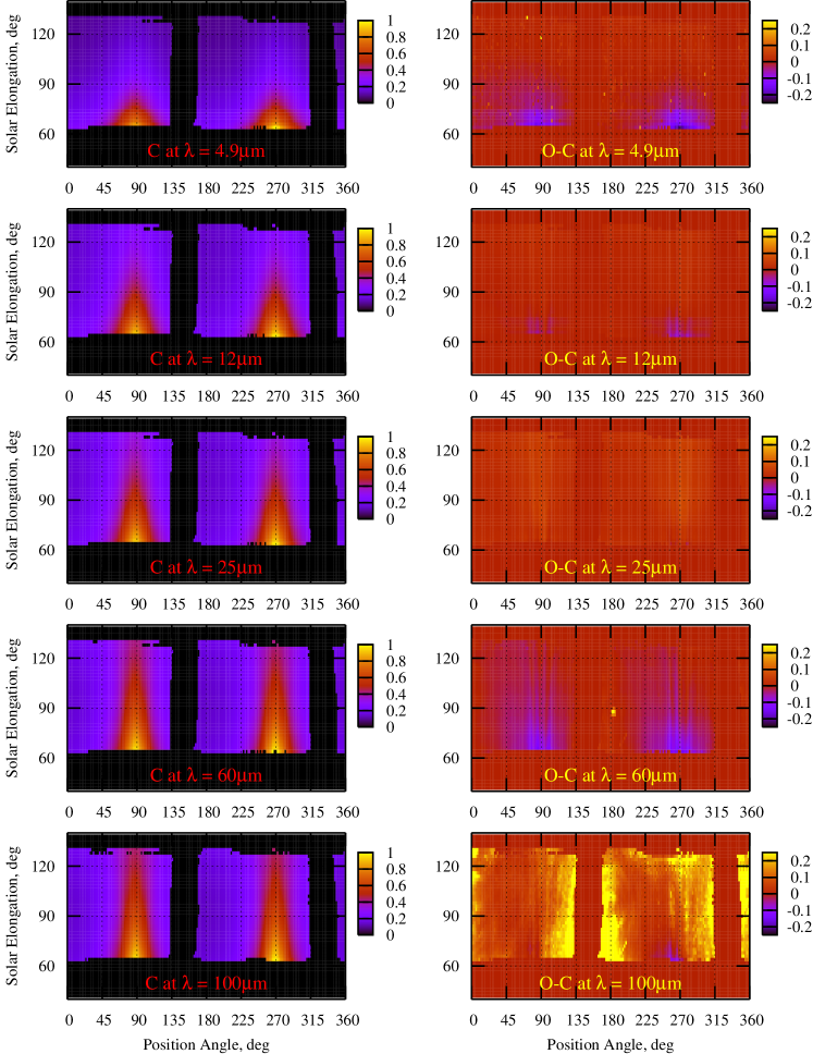
Figure 11: The best-fit model of the five COBE/DIRBE infrared sky maps (left), and its residuals, observations minus calculations (right), in relative units. Black areas on the left pannels are the forbidden zones of high and low solar elongation and the galactic plane excluded from the data set to avoid interference.

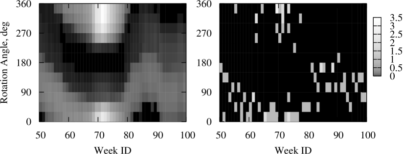
Figure 13: Impact counts with the Ulysses dust detector. Model expectations are on the left panel, actual counts are on the right panel. The time frame is chosen so that the first near-perihelion ecliptic plane crossing occurs on week 72.

The quality of the final fit can be assessed in Figures 11–13. The comparison with COBE observations is shown in Fig. 11. The infrared sky maps are constructed versus solar elongation and “position” angle with respect to the Sun. The latter is measured from the ecliptic north clockwise about the Earth-Sun axis. At the solar elongation of $90^{\circ}$, the position angle of $90^{\circ}$ is close to the apex of Earth motion, the position angle of $180^{\circ}$ is close to the vertex.

The agreement between data and theory is very good. For most pixels, the residual is below 10%. Some point sources not accounted by the interplanetary dust model are recognizable in the residual maps at the wavelengths 4.9 and 60 $\mu$m, while the map at 100 $\mu$m is polluted by the Milky Way that is still intensive near the band excluded along the Galaxy plane.

The spin-averaged impact rates on the Galileo dust detector (Fig. 12) are for the most time bins within the $1\sigma$ interval. The rates are dominated by the dust from comets and interstellar space, while the asteroids contribute less than 10% of impact events.

The impact counts with the dust detector of Ulysses are shown in Fig. 13. The impacts of interstellar dust grains occupy the range of rotation angles from 0 to $180^{\circ}$ and are seen as a zig-zag-shaped grey area in the lower part of the maps. Interplanetary dust impacts are dominant during the first near-perihelion ecliptic plane crossing that happened on week 72, the flux peak is at approximately $300^{\circ}$.

5.5 The model test against the independent data

The impact events collected by the dust detectors on board Helios 1 and Pioneer 11 satellites were of low statistical significance and have not been incorporated in the new meteoroid model. However, they can serve as an independent test of the model.

The Helios 1 spacecraft was launched into a highly eccentric orbit about the Sun with the aphelion at 1 AU and the perihelion at 0.3 AU. The orbital plane lay in the ecliptic plane (Grün, 1981). The spacecraft spinned about an axis perpendicular to that plane. Helios 1 made ten revolutions around the Sun over five years of operation, with two dust instruments registering dust impacts coming from the ecliptical plane and from the ecliptic south. The dust instruments measured, among other characteristics, the ion charge in the plasma cloud released by impacts. Although the detailed information on released charges has not survived the time, every impact in the records still available is marked by the ion charge range to which the charge belonged. The ion charge was related to the mass $m$ and speed $v$ of the impactor via the formula (Grün, 1981)

$$\left({Q_{\rm I}\over 1\;\mbox{C}}\right)\approx 4.07\cdot 10^{-5}\left({m\over 1\;\mbox{g}}\right)\cdot\left({v\over 1\;\mbox{km/s}}\right)^{2.7}.$$ (29)

We selected the impacts that fell in the ion charge ranges $\geq 2$ ($Q_{I}\geq 10^{-13}$ C) since the lowest range 1 appeared to be dominated by very small grains not described by the model quite well. The model expectations corrected for the “black-out” times ($\approx$39%) when the data were not transmitted from satellite, and the actual impact counts are shown in Fig. 14. The theoretical prediction remains within a factor of two to three of the measurements. The model predicts also a distinct feature of the local minimum of flux near the perihelion of the orbit of spacecraft that is absent from the data, although data statistics are rather poor. The local minimum is the consequence of the decrease of the average velocity of meteoroids relative to spacecraft causing the flux to fall as well. There is no such a minimum of the model predictions for the southern sensor.

When making predictions for the ecliptic sensor, the effect of a thin foil in its front was not taken into account, a necessary simplification that may explain why the model expectations are higher, and why the local minimum of flux is missing in the data while in the theory two maxima are present around zero mean anomaly. The ecliptic sensor was protected by the foil from the direct solar radiation, but the foil was also causing a bias by preferentially deflecting small and oblique impactors (Pailer and Grün, 1980).

The Pioneer 11 spacecraft was sent first to Jupiter, where it made a gravitational maneuver that deflected it into the path towards Saturn. Pioneer 11 carried penetration dust detector sensitive to relatively big meteoroids, $6\cdot 10^{-9}$ g at 20 km/s (Humes, 1980). The dust detector foil was punctured by the meteoroids satisfying the inequality

$$\left({m\over 1\;\mbox{g}}\right)\cdot\left({v\over 1\;\mbox{km/s}}\right)^{2.5}>10^{-5}.$$ (30)

The most intriguing result of this experiment was a flat penetration flux measured ever since the spacecraft left the asteroid belt behind. Although somewhat below the measured value, the flat rate is predicted by the new model too (Fig. 15). According to the meteoroid model, most of the impacts were due to the particles from comets, while the dust from asteroids and interstellar space contributed each less than 10% of observed fluxes. A discrepancy between the model prediction and the data seen in Fig. 15 for heliocentric distances larger than 5 AU can be explained by a dominant contribution from meteoroid sources beyond Jupiter (Landgraf et al., 2002).

5.6 Comparison with previous meteoroid models

The new meteoroid model differs essentially from the previous tools to predict particle fluxes on spacecraft in the way the orbital distributions of meteoroids are established. While Divine and Staubach used the observational data only to constrain the distributions, the new model comes with a wide set of meteoroid populations defined a-priori for a number of possible sources, evolving under the assumed dynamical laws. For instance, one name of meteoroid population, “asteroidal”, in the Divine model was referring solely to the proximity of the meteoroids to the asteroid belt, while in the new model the populations of dust from asteroids have genetic relationship to the main belt and prominent families.

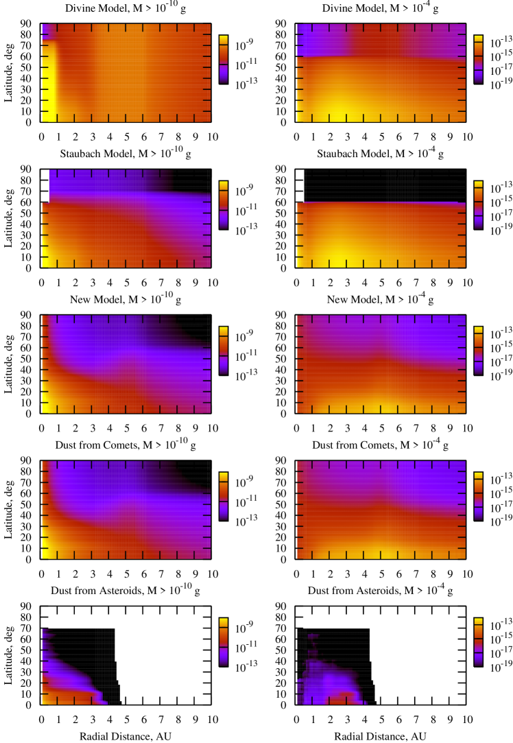
Figure 16: The number density (m^-3) of meteoroids above two mass thresholds, $10^{-10}$ g (left) and $10^{-4}$ g (right), predicted for the Divine, Staubach and the new models. For the new model, shown are also the number densities of meteoroids shed by comets and asteroids, respectively.

The evolution of models can be viewed in Fig. 16 where the number densities of meteoroids are mapped for wide ranges of heliocentric distances and latitudes above the ecliptic plane. Note that the number density at 1 AU in the ecliptic plane are similarly predicted by all models for the small grains distributed by the Poynting-Robertson effect. However, the new model specifies a substantially lower density at that location of the big grains controlled by gravity. In the new model, the majority of big particles are in Jupiter-crossing orbits, and their velocities are high with respect to the Earth and Moon. Therefore, in order to reproduce the lunar micro-crater frequencies, the new model needs a lower number density of meteoroids.

In the Divine model, a set of rectangular number density “patches” is most obvious, each of which corresponds to a single population having mathematically-separable distributions in perihelion distance, eccentricity and inclination, and therefore separable radial and latitudinal number density profiles. In the Staubach model predictions, manifestation of separability is mitigated by the logarithmic color scale, like in the Divine model predictions for the bigger meteoroids (logarithm of separable function is not necessarily separable).

In the new model, non-separability is imminent. Since the comets were represented by those on Jupiter-crossing orbits only, the number density of meteoroids peaks along the orbit of the giant planet. At the same heliocentric distance, the latitudinal number density profile is also widened. It looses breadth away from the Sun and down to the asteroid belt toward the Sun, from where it is extending in latitudes again (the effect is magnified greatly by the logarithmic scale but it is still real).

The asteroids are not separable as a source, too (see the plot for $M>10^{-4}$ g), so is the dust spiraling from them due to the Poynting-Robertson effect, until it leaves the source region. The ten-degree band due to the Eos and/or Veritas family is best revealed in the map of dust from asteroids, so it contributes a little density to the overall map as well.

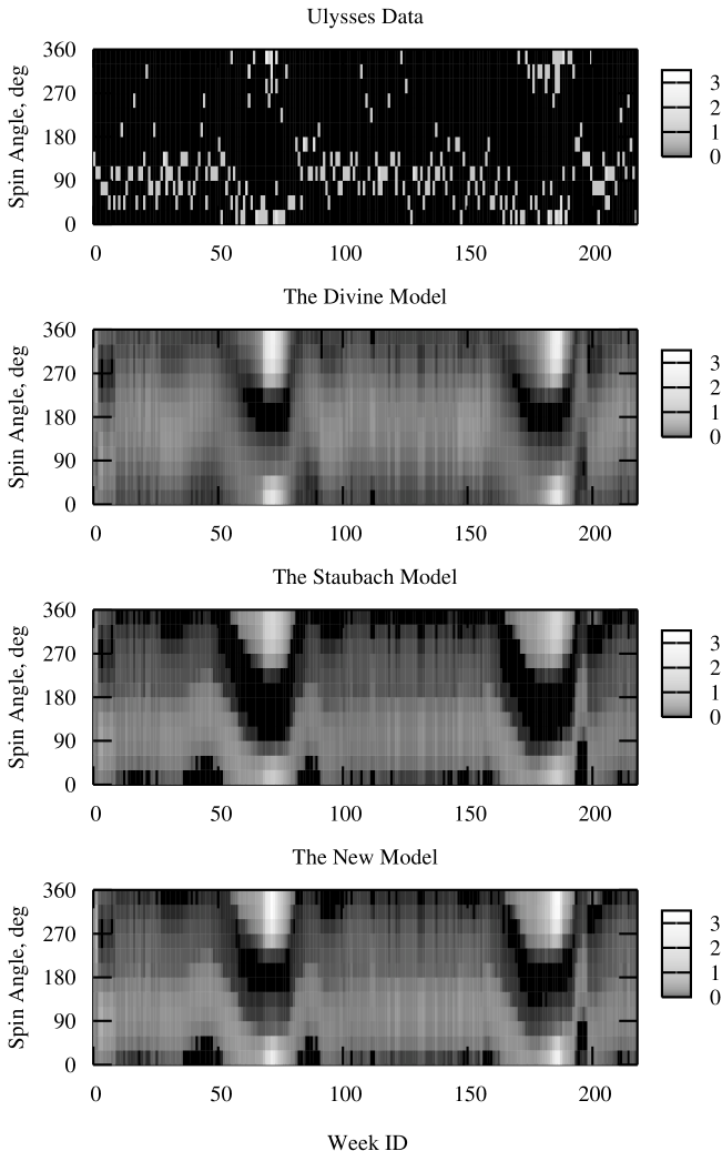
Figure 18: Impact counts reported by the Ulysses dust detector, for those weeks when at least one impact was detected, and their theoretical counterparts calculated using the Divine, Staubach, and the new models. The gray levels indicate the impact numbers.

By no surprise, the new meteoroid model is good or better at representation of those data sets incorporated. Interestingly, the Galileo DDS (Fig. 17) data are still reproduced by the Divine and Staubach models almost as good as by the new model, in spite of our revision of the DDS sensitivity threshold. The Divine model lacks the interstellar dust population that is obvious in the Ulysses data, however (Fig. 18). The information on spin angles of the Ulysses impacts not incorporated in the Divine model rejects Divine’s “halo” population that is dominant away from the ecliptic plane, e.g. week IDs 100–150. It is clearly seen that only the Staubach and new models give the right spin angle distributions of impacts during these periods.

It was intriguing to compare the performance of all models on those data that were not incorporated in the new model. Figures 19 and 20 show the three model predictions for the Helios 1 and Pioneer 11 impact records introduced in the previous section.

The Helios 1 data are described moderately good by both Divine’s and new model, although for the new model it is an extrapolation. The Staubach model predicts too low a flux, with the ecliptic sensor being dominated by the interstellar dust.

All three models show a perfect match with the Pioneer 11 data close to the Earth, however, once the spacecraft leaves the asteroid belt behind, they start to diverge. The Divine model stays the best description of this data set up to 6 AU from the Sun where we stop our inspection. In contrast, the Staubach model falls in significant contradiction with the data that were not the model’s base.

In fact, the Divine model explained the Pioneer 11 data by introducing a dedicated “halo” population with uniformly distributed orbital planes and low eccentricities. Although dynamically unstable on the time scale of several tens of Jovian revolutions about the Sun, this population fits well to the flat flux curve beyond the asteroid belt.

The new model, although being outside the 90% confidence interval after Jupiter fly-by, is still capable to reproduce the flat trend with a set of dynamically reasonable populations of dust from Jupiter-family comets. Lacking the Pioneer 11 data in its base, the new model shows the strength of the dynamical approach that powers extrapolations, an advantage that was missing in the previous models.

6 Conclusions

A new meteoroid model is developed to predict fluxes on spacecraft in the Solar system. In this model, the orbital evolution of meteoroids is for the first time taken into account in order to complement scarce data. The Poynting-Robertson effect, and the gravity of planets are taken into account to produce the orbital distributions of meteoroids from various known sources in the framework of approximate analytical solutions. These distributions are fitted to the infrared observations by the COBE/DIRBE instrument taken in five wavelength bands from 5 to 100 $\mu$m over the range of solar elongations from 60^∘ to 130^∘, the Galileo and Ulysses DDS in-situ flux measurements, and the micro-crater size frequencies counted on the lunar rock samples retrieved by the Apollo missions. The wall impacts into the DDS were first taken into account, the detector’s sensitivity to the big impacts was revised downwards by a factor 16 to reach an agreement with the COBE data. The AMOR orbital distributions could not be incorporated in the model since they fall in contradiction with the latitudinal number density profile of the zodiacal cloud behind the COBE infrared intensities and some earlier inversions of the zodiacal thermal and visual emissions. Improvements of the bias correction procedure or model assumptions, such as the constancy of material density, are required to fit to the AMOR and COBE data simultaneously.

Figure 1: The cumulative mass distributions of interplanetary meteoroids adopted in the new model.

Figure 2: The orbital distributions of asteroids and big meteoroids ($M>10^{-5}$ g).

Figure 3: The orbital distributions of small meteoroids ($M<10^{-5}$ g) from asteroids spiraling toward the Sun under the Poynting-Robertson effect.

Figure 4: The orbital distributions of the particles scattered gravitationally by a Jupiter-sized planet on a circular orbit 5.2 AU from the Sun. Dashed-lined step-functions are the results of numerical experiments, solid lines are the analytical solution.

Figure 5: Same as Fig. 4

Figure 6: The orbital distributions of the particles of a radius 10 $\mu$m leaking from the region of close encounters with Jupiter after being multiply scattered by this planet’s gravity. The gravity of major planets excepting Mercury and Pluto is taken into account. The solid curves show the analytics, the dashed-line step-functions are numerically accumulated statistics.

Figure 7: Same as Fig. 6.

Figure 8: The cumulative mass distribution of interstellar dust adopted in the new model.

Figure 9: The latitudinal number density profiles inferred from the infrared observations by IRAS (Clark et al., 1993), COBE (Kelsall et al., 1998), zodiacal light measurements (Leinert et al., 1981), and built based on the AMOR corrected orbital distributions (Galligan and Baggaley, 2004) at the distance 1 AU from the Sun.

Figure 10: Parameters of the final fit of the new meteoroid model. The three filled symbols show the weights of the three populations of dust from asteroids, spiraling under the Poynting-Robertson effect. The collisionally evolving populations are not shown since their weights are bound in the model to the corresponding Poynting-Robertson dust populations. The empty symbols depict the weights of the populations of dust from comets, both in the regime of encounters with Jupiter (with the collisional and Poynting-Robertson mass distributions above and below $M=10^{-5}$ g) and leaking from the region of encounters toward the Sun.

Figure 12: Impact rates measured by the Galileo dust detector, spin-averaged. Labels ‘V’, ‘E1’ and ‘E2’ mark one Venus and two Earth gravitational maneuvers, respectively.

Figure 14: Impact counts with the dust detectors on board Helios 1.

Figure 15: Fluxes inferred from the Pioneer 11 impact counts, taking the uncertainty of the number of active cells of dust detector into account (Dikarev and Grün, 2002) shown with error bars, and the meteoroid model expectation plotted as a continuous curve. On the heliocentric distance axis, ‘J’ marks the Jupiter fly-by, and ‘P’ marks the perihelion of the post-Jupiter orbit.

Figure 17: Impact rates measured by the Galileo dust detector, spin-averaged, and their theoretical counterparts calculated using the Divine, Staubach, and the new meteoroid models. Labels ‘V’, ‘E1’ and ‘E2’ mark one Venus and two Earth gravitational maneuvers, respectively.

Figure 19: Impact counts with the dust detectors on board Helios 1 and their theoretical counterparts calculated with the Divine, Staubach, and the new model.

Figure 20: Fluxes inferred from the Pioneer 11 impact counts (error bars), and their theoretical counterparts calculated using the Divine, Staubach, and the new model. Labels on the heliocentric distance axis are as in Fig. 15.

References

- Altobelli et al. (2004) Altobelli, N., H. Krüger, R. Moissl, M. Landgraf, and E. Grün 2004. Influence of wall impacts on the Ulysses dust detector on understanding the interstellar dust flux. Planet. Space Sci. 52, 1287–1295.
- Asada (1985) Asada, N. 1985. Fine fragments in high-velocity impact experiments. J. Geophys. Res. 90(9), 12445–12453.
- Baggaley (2001) Baggaley, W. J. 2001. The AMOR radar: an efficient tool for meteoroid research. Adv. Space Res. 28, 1277–1282.
- Boggess et al. (1992) Boggess, N. W., J. C. Mather, R. Weiss, C. L. Bennett, E. S. Cheng, E. Dwek, S. Gulkis, M. G. Hauser, M. A. Janssen, T. Kelsall, S. S. Meyer, S. H. Moseley, T. L. Murdock, R. A. Shafer, R. F. Silverberg, G. F. Smoot, D. T. Wilkinson, and E. L. Wright 1992. The COBE mission - Its design and performance two years after launch. Astrophys. J. 397, 420–429.
- Chambers (1999) Chambers, J. E. 1999. A hybrid symplectic integrator that permits close encounters between massive bodies. Mon. Not. R. Astron. Soc. 304, 793–799.
- Clark et al. (1993) Clark, F. O., M. V. Torbett, A. A. Jackson, S. D. Price, J. P. Kennealy, P. V. Noah, G. A. Glaudell, and M. Cobb 1993. The out-of-plane distribution of zodiacal dust near the earth. Astron. J. 105, 976–979.
- Cremonese et al. (1997) Cremonese, G., M. Fulle, F. Marzari, and V. Vanzani 1997. Orbital evolution of meteoroids from short period comets. Astron. Astrophys. 324, 770–777.
- Dermott et al. (2002) Dermott, S. F., T. J. J. Kehoe, D. D. Durda, K. Grogan, and D. Nesvorný 2002. Recent rubble-pile origin of asteroidal solar system dust bands and asteroidal interplanetary dust particles. In B. Warmbein (Ed.), Asteroids, Comets, and Meteors: ACM 2002 (ESA SP-500), pp. 319–322. ESTEC, Nordwijk, the Netherlands.
- Dermott et al. (1984) Dermott, S. F., P. D. Nicholson, J. A. Burns, and J. R. Houck 1984. Origin of the solar system dust bands discovered by IRAS. Nature 312, 505–509.
- Dikarev and Grün (2002) Dikarev, V., and E. Grün 2002. New information recovered from the Pioneer 11 meteoroid experiment data. Astron. Astrophys. 383, 302–308.
- Divine (1993) Divine, N. 1993. Five populations of interplanetary meteoroids. J. Geophys. Res. 98, 17029–17048.
- Everhart (1985) Everhart, E. 1985. An efficient integrator that uses Gauss-Radau spacings. In A. Carusi and B. Valsecchi (Eds.), Dynamics of Comets: Their Origin and Evolution, pp. 185–202. D. Reidel, Dordrecht.
- Galligan and Baggaley (2004) Galligan, D. P., and W. J. Baggaley 2004. The orbital distribution of radar-detected meteoroids of the Solar system dust cloud. Mon. Not. R. Astron. Soc. 353, 422–446.
- Gor’kavyi et al. (1997) Gor’kavyi, N. N., L. M. Ozernoy, J. C. Mather, and T. Taidakova 1997. Quasi-Stationary States of Dust Flows under Poynting-Robertson Drag: New Analytical and Numerical Solutions. Astrophys. J. 488, 268–276.
- Grogan et al. (1997) Grogan, K., S. F. Dermott, S. Jayaraman, and Y. L. Xu 1997. Origin of the ten degree Solar System dust bands. Planet. Space Sci. 45, 1657–1665.
- Grün et al. (1995) Grün, E., M. Baguhl, D. P. Hamilton, J. Kissel, D. Linkert, G. Linkert, and R. Riemann 1995. Reduction of Galileo and Ulysses dust data. Planet. Space Sci. 43, 941–951.
- Grün (1981) Grün, E. 1981. Physical and chemical characteristics of interplanetary dust particles—Measurements by the micrometeoroid experimenr on board Helios. Technical report, Max-Planck-Institut für Kernphysik.
- Grün et al. (1992a) Grün, E., H. Fechtig, M. S. Hanner, J. Kissel, D. Lindblad, B. A. Linkert, D. Maas, G. E. Morfill, and H. A. Zook 1992. The Galileo dust detector. Spa. Sci. Rev. 60, 317–340.
- Grün et al. (1992b) Grün, E., H. Fechtig, J. Kissel, D. Linkert, D. Maas, J. A. M. McDonnel, G. E. Morfill, G. Schwehm, H. A. Zook, and R. H. Giese 1992. The Ulysses dust experiment. Astron. Astrophys. Suppl. Series 92, 411–423.
- Grün et al. (1994) Grün, E., B. Gustafson, I. Mann, M. Baguhl, G. E. Morfill, P. Staubach, A. Taylor, and H. A. Zook 1994. Interstellar dust in the heliosphere. Astron. Astrophys. 286, 915–924.
- Grün et al. (1980) Grün, E., G. Morfill, G. Schwehm, and T. V. Johnson 1980. A model of the origin of the Jovian ring. Icarus 44, 326–338.
- Grün et al. (1997) Grün, E., P. Staubach, M. Baguhl, D. P. Hamilton, H. A. Zook, S. Dermott, B. A. Gustafson, H. Fechtig, J. Kissel, D. Linkert, G. Linkert, R. Srama, M. S. Hanner, C. Polanskey, M. Horányi, B. A. Lindblad, I. Mann, J. A. M. McDonnell, G. E. Morfill, and G. Schwehm 1997. South-North and Radial Traverses through the Interplanetary Dust Cloud. Icarus 129, 270–288.
- Grün et al. (1985) Grün, E., H. A. Zook, H. Fechtig, and R. H. Giese 1985. Collisional balance of the meteoritic complex. Icarus 62, 244–272.
- Hughes and McBride (1990) Hughes, D. W., and N. McBride 1990. The spatial density of large meteoroids in the inner solar system. Mon. Not. R. Astron. Soc. 243, 312–319.
- Humes (1980) Humes, D. H. 1980. Results of Pioneer 10 and 11 meteoroid experiments - Interplanetary and near-Saturn. J. Geophys. Res. 85, 5841–5852.
- Ishimoto (2000) Ishimoto, H. 2000. Modeling the number density distribution of interplanetary dust on the ecliptic plane within 5AU of the Sun. Astron. Astrophys. 362, 1158–1173.
- Kelsall et al. (1998) Kelsall, T., J. L. Weiland, B. A. Franz, W. T. Reach, R. G. Arendt, E. Dwek, H. T. Freudenreich, M. G. Hauser, S. H. Moseley, N. P. Odegard, R. F. Silverberg, and E. L. Wright 1998. The COBE Diffuse Infrared Background Experiment Search for the Cosmic Infrared Background. II. Model of the Interplanetary Dust Cloud. Astrophys. J. 508, 44–73.
- Landgraf et al. (2000) Landgraf, M., W. J. Baggaley, E. Grün, H. Krüger, and G. Linkert 2000. Aspects of the mass distribution of interstellar dust grains in the solar system from in situ measurements. J. Geophys. Res. 105(A5), 10343–10352.
- Landgraf et al. (2002) Landgraf, M., J.-C. Liou, H. A. Zook, and E. Grün 2002. Origins of Solar System dust beyond Jupiter. Astron. J. 123, 2857–2861.
- Laor and Draine (1993) Laor, A., and B. T. Draine 1993. Spectroscopic constraints on the properties of dust in active galactic nuclei. Astrophys. J. 402, 441–468.
- Leinert et al. (1981) Leinert, C., I. Richter, E. Pitz, and B. Planck 1981. The zodiacal light from 1.0 to 0.3 A.U. as observed by the HELIOS space probes. Astron. Astrophys. 103, 177–188.
- Leinert et al. (1983) Leinert, C., S. Roser, and J. Buitrago 1983. How to maintain the spatial distribution of interplanetary dust. Astron. Astrophys. 118, 345–357.
- Liou et al. (1999) Liou, J., H. A. Zook, and A. A. Jackson 1999. Orbital Evolution of Retrograde Interplanetary Dust Particles and Their Distribution in the Solar System. Icarus 141, 13–28.
- Liou et al. (1995) Liou, J. C., S. F. Dermott, and Y. L. Xu 1995. The contribution of cometary dust to the zodiacal cloud. Planet. Space Sci. 43, 717–722.
- Matney and Kessler (1996) Matney, M. J., and D. J. Kessler 1996. A Reformulation of Divine’s Interplanetary Model. In B. A. S. Gustafson and M. S. Hanner (Eds.), Physics, Chemistry and Dynamics of Interplanetary Dust (ASP Conf. Series 114), pp. 15–18.
- McDonnell (1978) McDonnell, J. A. M. 1978. Microparticle studies for space instrumentation. In J. A. M. MacDonnell (Ed.), Cosmic dust. Wiley-Interscience, Chichester.
- Pailer and Grün (1980) Pailer, N., and E. Grün 1980. The penetration limit of thin films. Planet. Space Sci. 28, 321–325.
- Price et al. (2003) Price, S. D., P. V. Noah, D. Mizuno, R. G. Walker, and S. Jayaraman 2003. Midcourse Space Experiment Mid-Infrared Measurements of the Thermal Emission from the Zodiacal Dust Cloud. Astron. J. 125, 962–983.
- Reach (1988) Reach, W. T. 1988. Zodiacal emission. I - Dust near the earth’s orbit. Astrophys. J. 335, 468–485.
- Staubach (1996) Staubach, P. 1996. Numerische Modellierung der Dynamik von Mikrometeoroiden und ihre Bedeutung für interplanetare Raumsonden und geozentrische Satelliten. Ph. D. thesis, Univ. of Heidelberg.
- Staubach et al. (1997) Staubach, P., E. Grün, and R. Jehn 1997. The meteoroid environment near earth. Adv. Space Res. 19, 301–308.
- Steel (1996) Steel, D. 1996. Meteoroid Orbits. Spa. Sci. Rev. 78, 507–553.
- Taylor (1995) Taylor, A. D. 1995. The Harvard Radio Meteor Project velocity distribution reappraised. Icarus 116, 154–158.
- Taylor and Elford (1998) Taylor, A. D., and W. G. Elford 1998. Meteoroid orbital element distributions at 1 AU deduced from the Harvard Radio Meteor Project observations. Earth Planets Space 50, 569–575.
- Wehry and Mann (1999) Wehry, A., and I. Mann 1999. Identification of -meteoroids from measurements of the dust detector onboard the ULYSSES spacecraft. Astron. Astrophys. 341, 296–303.
- Wilck and Mann (1996) Wilck, M., and I. Mann 1996. Radiation pressure forces on “typical” interplanetary dust grains. Planet. Space Sci. 44, 493–499.
- Witte et al. (1993) Witte, M., H. Rosenbauer, M. Banaszkiewicz, and H. Fahr 1993. The Ulysses neutral gas experiment - Determination of the velocity and temperature of the interstellar neutral helium. Adv. Space Res. 13, 121–130.
- Wyatt and Whipple (1950) Wyatt, S. P., and F. L. Whipple 1950. The Poynting-Robertson effect on meteor orbits. Astrophys. J. 111, 134–141.
- Zhu et al. (1997) Zhu, C., R. H. Byrd, and J. Nocedal 1997. L-BFGS-B: Algorithm 778: L-BFGS-B, FORTRAN routines for large scale bound constrained optimization. ACM Trans. on Math. Software 23(4), 550–560.