Synergistic Effects in Networked Epidemic Spreading Dynamics
Abstract
In this brief, we study epidemic spreading dynamics taking place in complex networks. We specifically investigate the effect of synergy, where multiple interactions between nodes result in a combined effect larger than the simple sum of their separate effects. Although synergistic effects play key roles in various biological and social phenomena, their analyses have been often performed by means of approximation techniques and for limited types of networks. In order to address this limitation, this paper proposes a rigorous approach to quantitatively understand the effect of synergy in the Susceptible-Infected-Susceptible model taking place in an arbitrary complex network. We derive an upper bound on the growth rate of the synergistic Susceptible-Infected-Susceptible model in terms of the eigenvalues of a matrix whose size grows quadratically with the number of the nodes in the network. We confirm the effectiveness of our result by numerical simulations on empirically observed human and animal social networks.
Index Terms:
Complex networks, spreading processes, synergistic interactions.I Introduction
Understanding epidemic spreading dynamics taking place in complex networks is of utmost importance with applications in epidemiology [1], opinion formation, rumor propagation, and cyber security [2, 3]. During the last two decades, several important advances have been made toward the analysis, modeling, and control of networked spreading processes [4]. For example, fundamental connections between the eigenvalues of a network and epidemic thresholds were identified in [5]. A unified framework for the analysis of spreading processes evolving on multilayer networks was presented in [6]. The dynamical change of network structures dependent on the evolution of spreading processes has been actively investigated in the context of adaptive networks [7]. Recently, control and optimization tools have been proven to be effective for containing spreading processes in static [8], multi-layer [9], and temporal [10] networks. A prominent example of the achievements of network epidemiology can be found in, for example, effective predictions of the pandemic of H1N1 influenza on 2009 [11, 12].
All the aforementioned results assume nearest-neighbor interactions, in which individual nodes are directly influenced by only their neighbors. However, in realistic epidemic spreading processes, we frequently observe multi-node interactions, in which a node can affect not only its neighbors but also other nodes such as the neighbors of its neighbors. A typical example of such phenomena can be found in the colonization by fungal and bacterial pathogens [13] and tumor growth [14]. In the context of human social networks, it has been experimentally confirmed that the spreads of opinions [15] and behaviors [16] are effectively accelerated by synergistic effects, which make the combined effect from multiple interactions greater than the simple sum of the effect of individual interactions.
We find in the literature several works providing theoretical insight for understanding the effect of synergistic interactions on spreading processes. The authors in [17] considered an extended Susceptible-Infected-Recovered (SIR) model with synergistic effects, and numerically confirmed on lattices that synergy can significantly alter asymptotic behaviors of the spread. Similar models were further investigated analytically on lattices [18] and small-world networks [19], respectively. The authors in [20] studied the effect of synergy in the Susceptible-Infected-Susceptible (SIS) model under the assumption that the nodes having the same degree behave in the same manner. The effect of synergy on deterministic spreading processes was investigated in [21] with a mean-field approximation technique.
This brief proposes a rigorous but tractable approach to quantitatively analyze the effect of synergy in the SIS model taking place in arbitrary networks, without resorting to mean-field approximations. A primary challenge in this context is to obtain computationally tractable results, because the state space of the spreading model grows exponentially with the number of nodes in the network. To overcome this difficulty, in this brief we show that the growth rate of the size of the infected population in the network can be bounded from above by the maximum real part of the eigenvalues of a matrix whose size grows only quadratically with the number of the nodes. In the derivation of the upper bound, we use Poisson-type stochastic differential equations describing the spreading model. The effectiveness of our theoretical results is numerically illustrated by simulations on empirical human and animal social networks.
This brief is organized as follows. After preparing mathematical notations, in Section II we introduce the synergistic SIS model over arbitrary complex networks. In Section III, we derive our upper-bound on the growth rate of the model. Numerical simulations are presented in Section IV.
Notations
The maximum real part of the eigenvalues of a square matrix is denoted by . An undirected graph is defined as the pair , where is a set of nodes and is a set of edges, i.e., unordered pairs of nodes. We say that nodes and are adjacent if . The neighborhood of node , denoted by , is defined as the set of nodes adjacent to node . The adjacency matrix of is defined as the matrix such that if nodes and are adjacent, and otherwise.
II Synergistic SIS model
We introduce the synergistic SIS model over complex networks in this section. Let us start by reviewing the standard SIS model without synergy (see, e.g., [22]). Let be an undirected graph having nodes labeled as , with edges representing interactions between nodes. At time , each node can be either susceptible or infected. When a node is infected, the node transitions into the susceptible state with an instantaneous rate . Also, if node is susceptible and has an infected neighbor, then the neighbor can infect node with an instantaneous rate . The rates and are called the recovery and transmission rate of node , respectively. We suppose that the above model evolves in the continuous-time; therefore, the rates represent probabilities per unit time [1] and, therefore, can be greater than one.
The SIS model uses a pair-wise description for infection events and, therefore, does not allow synergistic effects. In order to study the effect of synergy, we study the synergistic SIS model [23], which we describe below. In the model, while an infected node recovers with the rate as in the SIS model, the rate at which a susceptible node is infected by its infected neighbor, say, node , is equal to
| (1) |
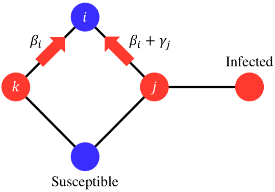
where denotes the strength of synergy and is dependent on individual nodes, and denotes the number of the infected neighbors of node at time . The second term in (1) is introduced to describe synergistic effects: a susceptible node is directly affected not only by its infected neighbors but also their neighbors (see Fig. 1 for a schematic picture). We remark that, according to the classification in [17], the synergistic SIS model incorporates only the d-synergies, which are caused by adjacent pairs of infected nodes. Due to the limitations of the space, this brief does not deal with the other category of synergies called r-synergies arising in the interactions between a susceptible node and its infected neighbors.
In this brief, we are interested in quantifying the rate at which the spreading process described by the synergistic SIS model grows. Therefore, we introduce the following definition:
Definition 1.
For all node and time , let denote the probability that node is infected at time . Define the growth rate of the synergistic SIS model by , where denotes the set of initially infected nodes.
In Definition 1, the sum represents the expected number of infected nodes. Therefore, the expression measures the asymptotic growth of the expected number of infected nodes. Hence, the growth rate in Definition 1 quantifies the worst-case growth of the average size of the infected population.
| (9) | ||||
| (10) |
The growth rate is closely related to fundamental notions in the network epidemiology such as mean-time-to-absorption [5] and epidemic thresholds [22]. However, it is hard in practice to exactly compute the growth rate. Since the synergistic SIS model, as a Markov process, has a total of states, the computation of the growth rate requires finding the eigenvalues of a matrix representing the infinitesimal generator of the Markov process [22]. Therefore, the computational complexity of exactly calculating the growth rate increases exponentially with the number of the nodes [24]. To overcome this difficulty, in the next section we introduce an upper-bound on the growth rate in terms of the eigenvalues of a matrix whose size grows only quadratically with .
III Growth rate
In this section, we derive an upper bound on the growth rate of the synergistic SIS model. For each node and time , let us define the variable as if node is infected at time , and otherwise. Then, since , the synergistic rate of infection (1) shows that the transition probability of the variable is described as and for . This implies that the variable obeys the following stochastic differential equation with Poisson jumps (see, e.g., [25]):
| (2) |
where , , and are independent Poisson counters with rates , , and , respectively. In the stochastic differential equation (2), the first, second, and third terms represent the recovery, direct infection from neighbors, and synergy effects.
By (2), the expectation satisfies
| (3) |
Notice that we have . Also, let us introduce the notations and for all and . Then, the differential equation (3) is rewritten as
| (4) |
This differential equation rigorously describes the evolution of the infection probabilities , which we require to compute the growth rate . However, the differential equation contains the higher-order terms and and, therefore, is not closed in the first-order term . For this reason, we cannot readily use the differential equation for calculating the growth rate.
We avoid this difficulty by ignoring the third order terms and deriving a set of differential inequalities for upper-bounding the growth rate of the synergistic SIS model. Intuitively, we can expect that ignoring the higher-order terms brings relatively small errors in the regime of extinction (i.e., when the epidemics dies out), in which lower-order terms become dominant. From differential equation (4), we obtain
| (5) |
It should be emphasized that, in deriving inequality (5), we chose to ignore the negative second order terms for as well as the third-order terms. We discuss the reason for and consequence from this manipulation later in Remark 2.
Then, let us derive differential equations for the evolution of the second-order terms. If we apply Itô’s formula [25] to the mapping and, then, take mathematical expectations in the resulting stochastic differential equation, we obtain
| (6) |
Since is -valued, the second term on the right-hand side of the differential equation (6) is bounded from above as . Likewise, the fifth term on the right-hand side of (6) can be bounded as . Furthermore, we have
| (7) |
These observations yield that
| (8) |
Remark 1.
One can derive different bounds on the derivative by replacing the reductions in (7) with others such as and . It is not theoretically easy to identify the best reduction giving the tightest bound on the derivative. However, we have numerically observed that using different reductions does not significantly alter the results of numerical simulations performed in Section IV.
By replacing second-order moments having indices with their equivalent counterparts , we rewrite the differential inequality (5) as (9) for all . In the same manner, we rewrite the differential inequality (8) as (10), which contains only the variables belonging to the set . Now, let denote the -dimensional vectorial variable that can be obtained by stacking the variables in the set . Then, we rewrite the system of differential inequalities (9) and (10) as
| (11) |
for a uniquely determined matrix .
Remark 2.
Since we ignored second order terms for deriving (5), one should expect a certain conservativeness in the bound (11) and, therefore, the bound of the decay rate to be later derived in Theorem 1. However, it is necessary to ignore the negative second order terms because, if not ignored, we cannot use the fact that the matrix is Metzler for the proof of the theorem.
Inequality (11) shows that, for all , there exists a nonnegative vector such that . From differential inequalities (9) and (10), we see that the off-diagonals of are nonnegative, i.e., is a Metzler matrix. This implies that the exponential has only nonnegative entries for all (see, e.g., [26]). Furthermore, by definition, each entry of the vector is nonnegative for all . Therefore, we obtain . This inequality bounds the vector , which contains the infection probabilities , …, , by the matrix exponential . We have thus proved the following theorem, which is the main theoretical result of this brief:
Theorem 1.
The growth rate of the synergistic SIS model satisfies .
IV Numerical simulations
In this section, we illustrate the effectiveness of Theorem 1 by numerical simulations. From Theorem 1, we can obtain a sufficient condition for the spreading process to become extinct (i.e., the spread is not invasive) as
| (12) |
This section is devoted to numerically validating the sufficiency of the extinction condition (12). To determine if the spreading process becomes extinct, we use the notion of the meta-stable number of infected nodes that is commonly used in the Network Science. To identify the meta-stable number of infected nodes, we begin by computing the following long-time average of the number of infected nodes for a sufficiently large . In simulations, the spreading process can die out due to random fluctuations. To prevent this from happening, we use the re-infection procedure [27] in which a randomly chosen node is infected immediately after the spreading process dies. After we finish the simulation, we determine the meta-stable number of infected nodes, denoted by , by
where we subtract one to compensate for the effect of the re-infection procedure. Finally, when , it is determined that the spreading process becomes extinct.
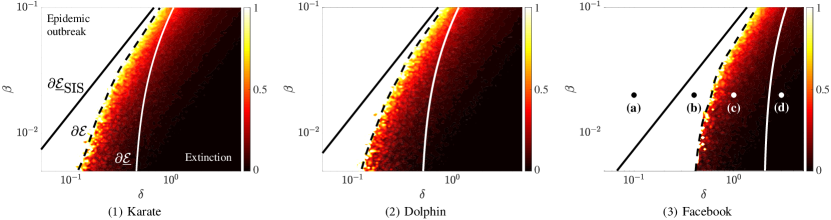
In our numerical simulations, we use the following three empirical human and animal social networks: (1) a social network of Zachary’s Karate club [28] (Karate, ), (2) a social network of bottlenose dolphins [29] (Dolphin, ), and (3) a friendship network in Facebook (Facebook, ). For simplicity of illustration, we assume that the network consists of homogeneous nodes; i.e., we assume , , and for constants , , and . In this numerical simulation, we fix . For the above three networks and various values of the transmission rate and the recovery rate , we compute the meta-stable number of infected nodes using the procedure described above, as well as our upper-bound on the growth rate. We then obtain the true extinction region
and its inner estimate from the sufficient condition (12):
In Fig. 3, we illustrate the regions and for the three empirical networks. We confirm that, for any of the networks, our inner-estimate is contained in the true extinction region (i.e., the boundary indicated by the white line passes through the colored region). For comparison, in Fig. 3, we also illustrate the estimate
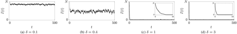
of the extinction region based on the conventional upper-bound on the growth rate of the SIS model without synergy [22]. Since the boundary passes outside the true extinction region for any of the three graphs, we observe that the use of the conventional method, which does not take into account synergistic effects, can lead to the overestimate of the extinction regions. In Fig. 3, we show sample paths of the time-evolution of the number of infected nodes for and , , , and . From Fig. 3.b, we confirm that the conventional method does overestimate the region of extinction.
V Conclusion
In this brief, we have studied the synergistic SIS model over arbitrary complex networks. Since the state space of the model grows exponentially fast with the number of nodes, it is almost impossible to directly analyze the model except when the network size is very small. To overcome this difficulty, we have derived an upper-bound on the growth rate the spreading model in terms of the eigenvalues of a matrix whose size grows quadratically with the number of the nodes. We have illustrated the effectiveness of our theoretical results by numerical simulations on empirical human and animal social networks. A possible direction for future research is eliminating the computational complexity for calculating our upper-bound. Since the size of grows quadratically, it is still not easy to apply the current bound for large-scale networks. It is of theoretical interest to examine if we can exploit the sparsity structure of to efficiently calculate the upper bound.
References
- [1] R. Pastor-Satorras, C. Castellano, P. Van Mieghem, and A. Vespignani, “Epidemic processes in complex networks,” Reviews of Modern Physics, vol. 87, pp. 925–979, 2015.
- [2] Y. Xia and D. J. Hill, “Attack vulnerability of complex communication networks,” IEEE Transactions on Circuits and Systems II: Express Briefs, vol. 55, pp. 65–69, 2008.
- [3] M. Babaei, H. Ghassemieh, and M. Jalili, “Cascading failure tolerance of modular small-world networks,” IEEE Transactions on Circuits and Systems II: Express Briefs, vol. 58, pp. 527–531, 2011.
- [4] C. Nowzari, V. M. Preciado, and G. J. Pappas, “Analysis and control of epidemics: A survey of spreading processes on complex networks,” IEEE Control Systems, vol. 36, pp. 26–46, 2016.
- [5] A. Ganesh, L. Massoulié, and D. Towsley, “The effect of network topology on the spread of epidemics,” in 24th Annual Joint Conference of the IEEE Computer and Communications Societies, 2005, pp. 1455–1466.
- [6] F. Darabi Sahneh, C. Scoglio, and P. Van Mieghem, “Generalized epidemic mean-field model for spreading processes over multilayer complex networks,” IEEE/ACM Transactions on Networking, vol. 21, pp. 1609–1620, 2013.
- [7] P. Zhu, Q. Zhi, Y. Guo, and Z. Wang, “Analysis of epidemic spreading process in adaptive networks,” IEEE Transactions on Circuits and Systems II: Express Briefs (Early Access). doi: 10.1109/TCSII.2018.2877406
- [8] V. M. Preciado, M. Zargham, C. Enyioha, A. Jadbabaie, and G. J. Pappas, “Optimal resource allocation for network protection against spreading processes,” IEEE Transactions on Control of Network Systems, vol. 1, pp. 99–108, 2014.
- [9] D. Zhao, B. Gao, Y. Wang, L. Wang, and Z. Wang, “Optimal dismantling of interdependent networks based on inverse explosive percolation,” IEEE Transactions on Circuits and Systems II: Express Briefs, vol. 65, pp. 953–957, 2018.
- [10] M. Ogura and V. M. Preciado, “Stability of spreading processes over time-varying large-scale networks,” IEEE Transactions on Network Science and Engineering, vol. 3, pp. 44–57, 2016.
- [11] D. Balcan et al., “Seasonal transmission potential and activity peaks of the new influenza A(H1N1): a Monte Carlo likelihood analysis based on human mobility.” BMC Medicine, vol. 7:45, 2009.
- [12] S. Merler, M. Ajelli, A. Pugliese, and N. M. Ferguson, “Determinants of the spatiotemporal dynamics of the 2009 h1n1 pandemic in europe: Implications for real-time modelling,” PLoS Computational Biology, vol. 7, 2011.
- [13] E. Ben-Jacob, O. Schochet, A. Tenenbaum, I. Cohen, A. Czirók, and T. Vicsek, “Generic modelling of cooperative growth patterns in bacterial colonies,” Nature, vol. 368, pp. 46–49, 1994.
- [14] L. A. Liotta and E. C. Kohn, “The microenvironment of the tumour–host interface,” Nature, vol. 411, pp. 375–379, 2001.
- [15] C. Castellano, S. Fortunato, and V. Loreto, “Statistical physics of social dynamics,” Reviews of Modern Physics, vol. 81, pp. 591–646, 2009.
- [16] D. Centola, “The spread of behavior in an online social network experiment,” Science, vol. 329, pp. 1194–1197, 2010.
- [17] F. J. Pérez-Reche, J. J. Ludlam, S. N. Taraskin, and C. A. Gilligan, “Synergy in spreading processes: from exploitative to explorative foraging strategies,” Physical Review Letters, vol. 106, p. 218701, 2011.
- [18] S. N. Taraskin and F. J. Pérez-Reche, “Effects of variable-state neighborhoods for spreading synergystic processes on lattices,” Physical Review E, vol. 88, p. 062815, 2013.
- [19] D. Broder-Rodgers, F. J. Pérez-Reche, and S. N. Taraskin, “Effects of local and global network connectivity on synergistic epidemics,” Physical Review E, vol. 92, p. 062814, 2015.
- [20] Q.-H. Liu, W. Wang, M. Tang, T. Zhou, and Y.-C. Lai, “Explosive spreading on complex networks: The role of synergy,” Physical Review E, vol. 95, p. 042320, 2017.
- [21] J. S. Juul and M. A. Porter, “Synergistic effects in threshold models on networks,” Chaos: An Interdisciplinary Journal of Nonlinear Science, vol. 28, p. 013115, 2018.
- [22] P. Van Mieghem, J. Omic, and R. Kooij, “Virus spread in networks,” IEEE/ACM Transactions on Networking, vol. 17, pp. 1–14, 2009.
- [23] J. J. Ludlam, G. J. Gibson, W. Otten, and C. A. Gilligan, “Applications of percolation theory to fungal spread with synergy,” Journal of The Royal Society Interface, vol. 9, pp. 949–956, 2012.
- [24] V. Y. Pan and Z. Q. Chen, “The complexity of the matrix eigenproblem,” in 31st Annual ACM Symposium on Theory of Computing. New York, New York, USA: ACM Press, 1999, pp. 507–516.
- [25] F. B. Hanson, Applied Stochastic Processes and Control for Jump-Diffusions: Modeling, Analysis and Computation. Society for Industrial and Applied Mathematics, 2007.
- [26] M. Ogura and V. M. Preciado, “Epidemic processes over adaptive state-dependent networks,” Physical Review E, vol. 93, p. 062316, 2016.
- [27] E. Cator, R. van de Bovenkamp, and P. Van Mieghem, “Susceptible-infected-susceptible epidemics on networks with general infection and cure times,” Physical Review E, vol. 87, p. 062816, 2013.
- [28] W. W. Zachary, “An information flow model for conflict and fission in small groups,” Journal of Anthropological Research, vol. 33, pp. 452–473, 1977.
- [29] J. Kunegis, “KONECT – the Koblenz network collection,” in Proceedings of the 22nd International Conference on World Wide Web, 2013, pp. 1343–1350.