Constraining DHOST theories with linear growth of matter density fluctuations

Abstract

We investigate the potential of cosmological observations, such as galaxy surveys, for constraining degenerate higher-order scalar-tensor (DHOST) theories, focusing in particular on the linear growth of the matter density fluctuations. We develop a formalism to describe the evolution of the matter density fluctuations during the matter dominated era and in the early stage of the dark energy dominated era in DHOST theories, and give an approximate expression for the gravitational growth index in terms of several parameters characterizing the theory and the background solution under consideration. By employing the current observational constraints on the growth index, we obtain a new constraint on a parameter space of DHOST theories. Combining our result with other constraints obtained from the Newtonian stellar structure, we show that the degeneracy between the effective parameters of DHOST theories can be broken without using the Hulse-Taylor pulsar constraint.

I Introduction

In the era of precision cosmology, one of the most significant problems is the elucidation of the origin of the late-time acceleration of the Universe Riess:1998cb ; Perlmutter:1998np . Modified gravity theories have been widely studied as an alternative to the most straightforward candidate of this origin, i.e., a cosmological constant. Among them, scalar-tensor theories with higher-order derivatives are receiving increasing attention. In general, such theories would have pathological extra ghost degrees of freedom because Ostrogradski’s theorem Ostro1 ; Woodard:2015zca requires that the equations of motion for a metric and a scalar field should be of second order to avoid such a ghost degree of freedom. A new wider class of healthy scalar-tensor theories with higher derivatives has been proposed recently and is called the degenerate higher-order scalar-tensor (DHOST) theories Langlois:2015cwa ; Crisostomi:2016czh ; Achour:2016rkg ; BenAchour:2016fzp , in which the equations of motion are of higher order, but one can reduce them to a second-order system due to the degeneracy (for a review, see Langlois:2017mdk ; Langlois:2018dxi ; Kobayashi:2019hrl ). DHOST theories include previously known scalar-tensor theories such as the Horndeski theory Horndeski:1974wa ; Deffayet:2011gz ; Kobayashi:2011nu , its disformal relatives Zumalacarregui:2013pma , and (a subclass of) the Gleyzes-Langlois-Piazza-Vernizzi (GLPV) theory Gleyzes:2014dya ; Gleyzes:2014qga . Then, it is intriguing to investigate observational and experimental constraints on these theories.

One of the most stringent constraints on gravity theories is obtained from the gravitational wave event GW170817 TheLIGOScientific:2017qsa and its optical counterpart GRB 170817A Monitor:2017mdv , which gave the constraint on the speed of gravitational waves, $c_{\rm GW}$, as $|c_{\rm GW}/c-1|\lesssim 10^{-15}$ with $c$ being the speed of light (hereafter we use units in which $c=1$). This observation can be used to rule out scalar-tensor theories which predict a variable gravitational-wave speed at low redshifts Lombriser:2015sxa ; Lombriser:2016yzn ; Creminelli:2017sry ; Sakstein:2017xjx ; Ezquiaga:2017ekz ; Baker:2017hug ; Langlois:2017dyl . One finds that there still is a broad class of viable scalar-tensor theories. In particular, a certain subclass of quadratic DHOST theories Langlois:2015cwa ; Crisostomi:2016czh ; Achour:2016rkg survived after this event.

Of course, even before GW170817 lots of stringent constraints on local gravity had been obtained, implying that gravity must be consistent with general relativity at least on small scales and in the weak gravity regime. Therefore, viable scalar-tensor theories are required to have a mechanism that suppresses the fifth force mediated by the scalar field on small scales, and Vainshtein screening is a typical one of such mechanisms in the Horndeski and related theories. Interestingly, DHOST theories generically exhibit Vainshtein screening outside matter, whereas its partial breaking occurs inside Kobayashi:2014ida ; Langlois:2017dyl ; Crisostomi:2017lbg ; Dima:2017pwp . As the gravitational laws inside an astrophysical body differ from the standard ones, this phenomenon leads to a modification of its internal structure, which can be used to constrain DHOST theories Saito:2015fza ; Sakstein:2015aac ; Jain:2015edg ; Babichev:2016jom ; Saltas:2018mxc ; Babichev:2018rfj . The authors of Ref. Dima:2017pwp applied this idea to the DHOST theories satisfying $c_{\rm GW}^{2}=1$ and obtained constraints on the parameters which characterize the theories.

In this paper, in addition to the above constraints, we investigate the possibility of constraining DHOST theories from the current/future precise cosmological observations. In particular, we focus on the linear evolution of the matter density fluctuations, which can be measured by observations of large scale structure. Measuring the linear growth rate of large-scale structure, $f(a)$, is known to be a powerful tool to test modifications of gravity responsible for the present cosmic acceleration. To compare the observational data with theoretical predictions, the simplest approach is to introduce an additional parameter called gravitational growth index, $\gamma$, defined in terms of the linear growth rate and the fraction parameter of non-relativistic matter $\Omega_{\rm m}$ as Wang:1998gt

$$\gamma:=\frac{{\rm d}\ln f}{{\rm d}\ln\Omega_{\rm m}}.$$ (1)

The purpose of this paper is to obtain a novel constraint on DHOST theories with $c_{\rm GW}^{2}=1$ from the observations of the linear growth rate. To do so, we develop a formalism to describe DHOST cosmology during the matter dominated era and the early stage of the dark energy dominated era, and evaluate the growth index at high redshifts. We expect that the current observations of the growth index yield new constraints on DHOST theories which are complementary to the existing bounds.

The paper is organized as follows. In Sec. II, we derive cosmological background equations in class I quadratic DHOST theories. Then we consider linear cosmological perturbations and derive the evolution equation of the density fluctuations. In Sec. III, we introduce our formalism to model DHOST cosmology and evaluate the growth index as a probe of modifications gravity. We thereby give novel constraints on DHOST theories from current observations. Finally, we discuss our results and future prospects in Sec. V.

II DHOST theories: background and perturbation equations

II.1 Action

The action of the quadratic DHOST theories Langlois:2015cwa ; Crisostomi:2016czh is given by

$$S=\int{\rm d}^{4}x\sqrt{-g}\left[G_{2}(\phi,X)-G_{3}(\phi,X)\Box\phi+G_{4}(\phi,X)R+\sum^{5}_{i=1}a_{i}(\phi,X)L_{i}\right],$$ (2)

where we have several functions of the scalar field $\phi$ and its kinetic term $X:=(-1/2)\phi_{\mu}\phi^{\mu}$. The Lagrangians $L_{i}$ are quadratic in the second derivatives of $\phi$ and are given by

$$L_{1}=\phi_{\mu\nu}\phi^{\mu\nu},\quad L_{2}=(\Box\phi)^{2},\quad L_{3}=(\Box\phi)\phi^{\mu}\phi_{\mu\nu}\phi^{\nu},\quad L_{4}=\phi^{\mu}\phi_{\mu\rho}\phi^{\rho\nu}\phi_{\nu},\quad L_{5}=(\phi^{\mu}\phi_{\mu\nu}\phi^{\nu})^{2},$$ (3)

where $\phi_{\mu}:=\nabla_{\mu}\phi$ and $\phi_{\nu\rho}:=\nabla_{\rho}\nabla_{\nu}\phi$.

In order for this higher-derivative theory to be free of Ostrogradsky ghosts, we must impose the degeneracy conditions that relate $G_{4}$ and $a_{i}$. The quadratic DHOST theories are classified in several subclasses Langlois:2015cwa ; Crisostomi:2016czh , among which we are interested in the so-called class I theories, because theories in other subclasses exhibit some pathologies in a cosmological setup deRham:2016wji ; Langlois:2017mxy . (The class I DHOST theories are conformally/disformally related to the Horndeski theory Achour:2016rkg ; Crisostomi:2016czh .) The class I degeneracy conditions are summarized as

$$a_{1}+a_{2}=0,\quad\beta_{2}=-6\beta_{1}^{2},\quad\beta_{3}=-2\beta_{1}\left[2(1+\alpha_{\rm H})+\beta_{1}(1+\alpha_{\rm T})\right],$$ (4)

where

$$M^{2}=2(G_{4}+2Xa_{1}),\quad M^{2}\alpha_{\rm T}=-4Xa_{1},\quad M^{2}\alpha_{\rm H}=-4X(G_{4X}+a_{1}),$$

$$M^{2}\beta_{1}=2X(G_{4X}-a_{2}+Xa_{3}),\quad M^{2}\beta_{2}=4X[a_{1}+a_{2}-2X(a_{3}+a_{4})+4X^{2}a_{5}],$$

$$M^{2}\beta_{3}=-8X(G_{4X}+a_{1}-Xa_{4}).$$ (5)

Here we write the derivative of a function $f(X)$ with respect to $X$ as $f_{X}$. We thus have 3 constraints among 6 functions ($G_{4}$ and $a_{i}$), leaving 3 free functions in addition to $G_{2}$ and $G_{3}$.

Note that the propagation speed of gravitational waves is given by $c_{\rm GW}^{2}=1+\alpha_{\rm T}$. The gravitational wave event GW170817 TheLIGOScientific:2017qsa and its optical counterpart GRB 170817A Monitor:2017mdv have placed a tight bound $c_{\rm GW}^{2}\simeq 1$. We therefore have $\alpha_{\rm T}\simeq 0$, provided that this constraint is valid at low energies where dark energy/modified gravity models are used deRham:2018red . Imposing $\alpha_{\rm T}=0$ amounts to taking $a_{1}=a_{2}=0$, but for the moment we do not require this.

II.2 Background equations in shift-symmetric DHOST theories

In the rest of the paper we focus on the shift-symmetric subclass of DHOST theories, in which the Lagrangian is invariant under a constant shift of the scalar field, namely $\phi\to\phi+\,$const. This means that the free functions contained in the Lagrangian are dependent only on the scalar field kinetic term $X$.

As a matter component we only consider pressureless dust and assume that it is minimally coupled to gravity. For a homogeneous and isotropic background, ${\rm d}s^{2}=-{\rm d}t^{2}+a^{2}(t)\delta_{ij}{\rm d}x^{i}{\rm d}x^{j}$, $\phi=\phi(t)$, with the matter energy density $\rho_{\rm m}$, the gravitational field equations read

$$3M^{2}H^{2} =\rho_{\rm m}+\rho_{\phi},$$ (6)

$$-M^{2}\left(2\dot{H}+3H^{2}\right) =p_{\phi},$$ (7)

where $H=\dot{a}/a$ (a dot denotes differentiation with respect to $t$), and

$$\rho_{\phi} :=\dot{\phi}{\cal J}-G_{2}-M^{2}H^{2}\left(6\beta_{1}y-\frac{1}{2}\beta_{2}y^{2}\right),$$ (8)

$$p_{\phi} :=G_{2}+2M^{2}H^{2}\left[(\alpha_{\rm B}+3\beta_{1})y-\left(\beta_{1}+\frac{\beta_{2}}{4}\right)y^{2}\right]+2M^{2}\beta_{1}\frac{{\rm d}}{{\rm d}t}\left(yH\right),$$ (9)

with ${\cal J}$ being the shift current defined shortly. Here we defined $y:=\ddot{\phi}/(H\dot{\phi})$ and

$$\alpha_{\rm M} :=\frac{1}{M^{2}H}\frac{{\rm d}M^{2}}{{\rm d}t},$$ (10)

$$\alpha_{\rm B} :=-\frac{\dot{\phi}XG_{3X}}{M^{2}H}+\frac{\alpha_{\rm H}}{y}-\left(3-\alpha_{\rm M}\right)\beta_{1}+\frac{\dot{\beta}_{1}}{H}+\left(\beta_{1}+\frac{\beta_{2}}{2}\right)y.$$ (11)

The scalar field equation can be written using the shift current as

$$\dot{\cal J}+3H{\cal J}=0,$$ (12)

where

$$\dot{\phi}{\cal J} =2XG_{2X}+M^{2}H^{2}\left[\frac{3\alpha_{\rm M}}{y}-6\alpha_{\rm B}+6\left(\alpha_{\rm M}\beta_{1}+\frac{\dot{\beta}_{1}}{H}\right)+6\beta_{1}y-\frac{1}{2}\left(\alpha_{\rm M}\beta_{2}+\frac{\dot{\beta}_{2}}{H}\right)y\right]$$

$$\quad+6M^{2}\beta_{1}\dot{H}-M^{2}\beta_{2}\frac{{\rm d}}{{\rm d}t}\left(yH\right).$$ (13)

Equation (12) implies that in the expanding Universe ${\cal J}={\rm const}/a^{3}\to 0$ and hence attractor solutions are characterized by ${\cal J}=0$.

The background equations (6), (7), and (12) contain the higher derivatives $\dddot{\phi}$, $\ddddot{\phi}$, and $\ddot{H}$. However, the degeneracy conditions (4) allow us to reduce the system to the second-order one. It is not so obvious to demonstrate this explicitly, but one can follow Refs. Crisostomi:2017pjs ; Crisostomi:2018bsp to see that it is indeed possible to do so.

II.3 Density perturbations

Let us study matter density fluctuations in the Newtonian gauge. The perturbed metric in the Newtonian gauge is given by

$${\rm d}s^{2}=-\left[1+2\Phi(t,{\bm{x}})\right]{\rm d}t^{2}+a^{2}(t)\left[1-2\Psi(t,{\bm{x}})\right]\delta_{ij}{\rm d}x^{i}{\rm d}x^{j}.$$ (14)

We write the perturbation of the scalar field as

$$\phi(t,{\bm{x}})=\phi(t)+\pi(t,{\bm{x}}).$$ (15)

It is convenient to introduce a dimensionless variable $Q:=H\pi/\dot{\phi}$, and we will use this instead of $\pi$. The density perturbation is defined by

$$\rho_{\rm m}(t,{\bm{x}})=\overline{\rho}_{\rm m}(t)[1+\delta(t,{\bm{x}})].$$ (16)

We study the quasi-static evolution of the perturbations inside the sound horizon scale. The quasi-static approximation indicates that $\dot{\epsilon}\sim H\epsilon\ll\partial\epsilon$, where $\epsilon$ is any of perturbation variables. Expanding the action to second order in perturbations under the quasi-static approximation, we obtain the following effective action:

$$S_{\mathrm{eff}}=\int{\rm d}^{4}x\,{\cal L}_{\mathrm{eff}},$$ (17)

with

$${\cal L}_{\rm eff} =\frac{M^{2}a}{2}\Biggl{\{}(c_{1}\Phi+c_{2}\Psi+c_{3}Q)\partial^{2}Q+4(1+\alpha_{\rm H})\Psi\partial^{2}\Phi-2(1+\alpha_{\rm T})\Psi\partial^{2}\Psi$$

$$\quad-\beta_{3}\Phi\partial^{2}\Phi+\biggl{[}4\alpha_{\rm H}\frac{\dot{\Psi}}{H}-2(2\beta_{1}+\beta_{3})\frac{\dot{\Phi}}{H}+(4\beta_{1}+\beta_{3})\frac{\ddot{Q}}{H^{2}}\biggr{]}\partial^{2}Q\Biggr{\}}-a^{3}\overline{\rho}_{\mathrm{m}}\Phi\delta,$$ (18)

where

$$c_{1} :=-4\left[\alpha_{\rm B}-\alpha_{\rm H}+\frac{\beta_{3}}{2}(1+\alpha_{\rm M})+\frac{\dot{\beta}_{3}}{2H}\right],$$ (19)

$$c_{2} :=4\left[\alpha_{\rm H}(1+\alpha_{\rm M})+\alpha_{\rm M}-\alpha_{\rm T}+\frac{\dot{\alpha}_{\rm H}}{H}\right],$$ (20)

$$c_{3} :=-2\Bigg{\{}\left(1+\alpha_{\rm M}+\frac{\dot{H}}{H^{2}}\right)\left(\alpha_{\rm B}-\alpha_{\rm H}\right)+\frac{\dot{\alpha}_{\rm B}-\dot{\alpha}_{\rm H}}{H}+\frac{3\Omega_{\rm m}}{2}+\frac{\dot{H}}{H^{2}}+\alpha_{\rm T}-\alpha_{\rm M}$$

$$\quad+\left[-2\frac{\dot{H}}{H^{2}}\beta_{1}+\frac{\beta_{3}}{4}(1+\alpha_{\rm M})+\frac{\dot{\beta}_{3}}{2H}\right]\left(1+\alpha_{\rm M}-\frac{\dot{H}}{H^{2}}\right)-2\frac{\dot{H}}{H^{2}}\frac{\dot{\beta}_{1}}{H}+\left(\frac{\dot{H}}{H^{2}}\right)^{2}\frac{\beta_{3}}{2}+\frac{\dot{\alpha}_{\rm M}}{H}\frac{\beta_{3}}{4}+\frac{\ddot{\beta}_{3}}{4H^{2}}\Bigg{\}},$$ (21)

and

$$\Omega_{\rm m} :=\frac{\overline{\rho}_{\rm m}}{3M^{2}H^{2}}.$$ (22)

We have three terms whose coefficients are written solely in terms of $\beta_{1}$ and $\beta_{3}$. (The latter can be expressed in terms of $\alpha_{\rm H}$, $\alpha_{\rm T}$, and $\beta_{1}$ using the degeneracy condition given by Eq. (4).) These are the new terms in DHOST theories. The other terms are present in the Horndeski and GLPV theories, but as $c_{1}$ and $c_{3}$ are dependent on $\beta_{1}$ and $\beta_{3}$ one can see implicitly the contributions of these parameters characterizing DHOST theories.

The field equations are derived by varying the effective action with respect to $\Phi$, $\Psi$, and $Q$. Going to Fourier space, they are given by

$$(1+\alpha_{\rm H})\Psi-\frac{\beta_{3}}{2}\Phi+b_{1}Q+\frac{2\beta_{1}+\beta_{3}}{2}\frac{\dot{Q}}{H}+\frac{a^{2}}{2M^{2}k^{2}}\overline{\rho}_{\rm m}\delta =0,$$ (23)

$$(1+\alpha_{\rm T})\Psi-(1+\alpha_{\rm H})\Phi+b_{2}Q+\alpha_{\rm H}\frac{\dot{Q}}{H} =0,$$ (24)

$$c_{2}\Psi+c_{1}\Phi+b_{3}Q+4\alpha_{\rm H}\frac{\dot{\Psi}}{H}-2(2\beta_{1}+\beta_{3})\frac{\dot{\Phi}}{H}+b_{4}\frac{\dot{Q}}{H}+2(4\beta_{1}+\beta_{3})\frac{\ddot{Q}}{H^{2}} =0,$$ (25)

where $k$ denotes a comoving wavenumber in Fourier space and $\Phi$, $\Psi$, and $Q$ are now understood as the Fourier components. Here, the coefficients $b_{i}$ ($i=1,2,3,4$) are defined as

$$b_{1} :=\frac{c_{1}}{4}+\frac{1}{2}(1+\alpha_{\rm M})(2\beta_{1}+\beta_{3})+\frac{1}{2}\frac{{\rm d}}{{\rm d}t}\left(\frac{2\beta_{1}+\beta_{3}}{H}\right),$$ (26)

$$b_{2} :=-\frac{c_{2}}{4}+(1+\alpha_{\rm M})\alpha_{\rm H}+\frac{{\rm d}}{{\rm d}t}\left(\frac{\alpha_{\rm H}}{H}\right),$$ (27)

$$b_{3} :=2c_{3}+\left[\left(1+\alpha_{\rm M}-\frac{\dot{H}}{H^{2}}\right)(1+\alpha_{\rm M})+\frac{\dot{\alpha}_{\rm M}}{H}\right](4\beta_{1}+\beta_{3})$$

$$\quad+2(1+\alpha_{\rm M})\frac{{\rm d}}{{\rm d}t}\left(\frac{4\beta_{1}+\beta_{3}}{H}\right)+\frac{{\rm d}^{2}}{{\rm d}t^{2}}\left(\frac{2\beta_{1}+\beta_{3}}{H^{2}}\right),$$ (28)

$$b_{4} :=2\Biggl{[}\left(1+\alpha_{\rm M}-\frac{\dot{H}}{H^{2}}\right)(4\beta_{1}+\beta_{3})+\frac{{\rm d}}{{\rm d}t}\left(\frac{4\beta_{1}+\beta_{3}}{H}\right)\Biggr{]}.$$ (29)

Since matter is assumed to be minimally coupled to gravity, the fluid equations are the same as the standard ones, and hence under the quasi-static approximation the matter density fluctuations $\delta(t,{\bm{x}})$ and the velocity field $u^{i}(t,{\bm{x}})$ obey

$$\dot{\delta}+\frac{1}{a}\partial_{i}[(1+\delta)u^{i}]=0,$$ (30)

$$\dot{u}^{i}+Hu^{i}+\frac{1}{a}u^{j}\partial_{j}u^{i}=-\frac{1}{a}\partial^{i}\Phi.$$ (31)

At linear order, these equations are combined to give

$$\ddot{\delta}+2H\dot{\delta}+{k^{2}\over a^{2}}\Phi=0,$$ (32)

where we moved to Fourier space. The effects of modified gravity come into play through the gravitational potential $\Phi$ which is determined by solving Eqs. (23)–(25).

Let us then solve Eqs. (23)–(25) to express $\Phi$, $\Psi$, and $Q$ in terms of $\delta$ and its time derivatives. We will follow the same procedure as that used in Hirano:2018uar . This procedure is feasible thanks to the degeneracy of the theory. Solving Eqs. (23) and (24) for $\Phi$ and $\Psi$ and substituting these solutions into Eq. (25), one finds that $\ddot{Q}$ and $\dot{Q}$ terms are canceled due to the degeneracy, and hence $Q$ can be expressed in the form

$$-\frac{k^{2}}{a^{2}H^{2}}Q =\kappa_{Q}\delta+\nu_{Q}\frac{\dot{\delta}}{H},$$ (33)

where the explicit expressions for the time-dependent coefficients $\kappa_{Q}$ and $\nu_{Q}$ are presented in Appendix A. Finally, substituting this back into Eqs. (23) and (24), the gravitational potentials $\Phi$ and $\Psi$ can be expressed in terms of $\delta$, $\dot{\delta}$, and $\ddot{\delta}$ as

$$-\frac{k^{2}}{a^{2}H^{2}}\Phi =\kappa_{\Phi}\delta+\nu_{\Phi}\frac{\dot{\delta}}{H}+\mu_{\Phi}\frac{\ddot{\delta}}{H^{2}},$$ (34)

$$-\frac{k^{2}}{a^{2}H^{2}}\Psi =\kappa_{\Psi}\delta+\nu_{\Psi}\frac{\dot{\delta}}{H}+\mu_{\Psi}\frac{\ddot{\delta}}{H^{2}}.$$ (35)

The explicit expressions for the time-dependent coefficients $\mu_{i}$, $\nu_{i}$, and $\kappa_{i}$ ($i=\Phi,\Psi$) are also shown in Appendix A. Within the Horndeski theory we have $\mu_{i}=\nu_{i}=0$ and in the GLPV theory we still have $\mu_{\Psi}=0$. That is, $\mu_{\Psi}$ first appears in DHOST theories beyond GLPV. Equation (34) allows us to eliminate $\Phi$ from Eq. (32) and we obtain the closed-form equation for $\delta$ as

$$\ddot{\delta}+(2+\varsigma)H\dot{\delta}-\frac{3}{2}\Omega_{\mathrm{m}}\Xi_{\Phi}H^{2}\delta=0,$$ (36)

where the additional friction $\varsigma$ and the effective gravitational coupling (multiplied by $8\pi M^{2}$) $\Xi_{\Phi}$ are written in terms of $\mu_{\Phi}\,,\nu_{\Phi}$ , and $\kappa_{\Phi}$ as

$$\varsigma =\frac{2\mu_{\Phi}-\nu_{\Phi}}{1-\mu_{\Phi}}\,,$$ (37)

$$\Xi_{\Phi} =\frac{2}{3\Omega_{\rm m}}\frac{\kappa_{\Phi}}{1-\mu_{\Phi}}\,.$$ (38)

These two functions characterize modification of gravity. The evolution equation (36) has essentially the same form as that in DHOST theories with $c_{\rm GW}^{2}=1$ Crisostomi:2017pjs and in the GLPV theory Gleyzes:2014qga ; DAmico:2016ntq . Whether or not $c_{\rm GW}^{2}=1$ does not play an important role in determining the qualitative form of Eq. (36). In the case of the Horndeski theory ($\alpha_{\rm H}=\beta_{1}=0$), the additional friction term vanishes, $\varsigma=0$, and the result of Ref. DeFelice:2011hq is recovered.

Equation (36) tells us that, even in DHOST theories under the quasi-static approximation, the evolution of the matter density fluctuations is independent of the wavenumber, so that as usual we can write the growing solution to Eq. (36) as

$$\delta(t,{\bf k})=D_{+}(t)\delta_{\rm L}({\bf k}),$$ (39)

where $\delta_{\rm L}({\bf k})$ represents the initial density field. The effect of the modified evolution of the density perturbations is thus imprinted in the growth factor, $D_{+}(t)$. Introducing the linear growth rate, $f:={\rm d}\ln D_{+}/{\rm d}\ln a$, the evolution equation can be written as

$$\frac{{\rm d}f}{{\rm d}\ln{a}}+\left(2+\varsigma+\frac{{\rm d}\ln{H}}{{\rm d}\ln{a}}\right)f+f^{2}-\frac{3}{2}\Omega_{\rm m}\Xi_{\Phi}=0.$$ (40)

Given the expansion history and the dynamics of the scalar field, one can obtain the evolution of the linear growth rate by solving the above equation.

III Modeling DHOST cosmology in the matter dominated era

We consider possible cosmological constraints on DHOST theories from observables during the matter dominated era and in the early stage of the dark energy dominated era. To do so, we assume that during these stages $y$, $G_{2}$, $\alpha_{i}$ ($i=$H, M, B, T), and $\beta_{1}$ can be expressed as a series expansion form in terms of $\varepsilon:=1-\Omega_{\rm m}\,(\ll 1)$ as

$$y =y_{0}+{\cal O}(\varepsilon),$$ (41)

$$G_{2} =g_{2}M^{2}H^{2}\varepsilon+{\cal O}\left(\varepsilon^{2}\right),$$ (42)

$$\alpha_{i} =c_{i}\varepsilon+{\cal O}\left(\varepsilon^{2}\right),$$ (43)

$$\beta_{1} =\beta\varepsilon+{\cal O}\left(\varepsilon^{2}\right),$$ (44)

where $y_{0}$, $g_{2}$, $c_{i}$, and $\beta$ are constants. Note that the expansion of $\alpha_{i}$ and $\beta_{1}$ starts at ${\cal O}(\varepsilon)$, as modifications of gravity are supposed not to be significant at early times. As seen below, the background equations are consistent with Eqs. (41)–(44). The expansion coefficients $(y_{0},g_{2},c_{i},\beta)$ are not all independent parameters. We will express some of them in terms of the other coefficients and the parameters of an underlying model.

Substituting Eqs. (41)–(44) to Eqs. (8) and (9), one finds, for the attractor solutions (${\cal J}=0$), that

$$\rho_{\phi} =-\left(g_{2}+6\beta y_{0}\right)M^{2}H^{2}\varepsilon+{\cal O}\left(\varepsilon^{2}\right),$$ (45)

$$p_{\phi} =\Bigl{[}g_{2}+2\bigl{(}c_{\rm B}+3\beta\bigr{)}y_{0}-2\beta y^{2}_{0}\,\Bigr{]}M^{2}H^{2}\varepsilon+2M^{2}\beta y_{0}\dot{H}\varepsilon+{\cal O}\left(\varepsilon^{2}\right).$$ (46)

Noting that $3M^{2}H^{2}-\bar{\rho}_{\rm m}=3M^{2}H^{2}\varepsilon=\rho_{\phi}$, we have

$$g_{2}=-3\left(1+2\beta y_{0}\right).$$ (47)

The effective dark energy equation of state parameter, $w_{\phi}:=p_{\phi}/\rho_{\phi}$, can be expanded as

$$w_{\phi}=w^{(0)}+{\cal O}(\varepsilon).$$ (48)

From Eqs. (45)–(47) and $\dot{H}/H^{2}=-3/2+{\cal O}(\varepsilon)$ we obtain

$$w^{(0)}=-1+\frac{2}{3}\left(c_{\rm B}y_{0}-\frac{3}{2}\beta y_{0}-\beta y^{2}_{0}\right).$$ (49)

Using the above expression for $w^{(0)}$, one has the following useful formulas valid up to ${\cal O}(\varepsilon)$:

$$\frac{\dot{H}}{H^{2}}=-\frac{3}{2}\left(1+w^{(0)}\varepsilon\right)+{\cal O}(\varepsilon^{2}),\quad\frac{\dot{\varepsilon}}{H}=\left(c_{\rm M}-3w^{(0)}\right)\varepsilon+{\cal O}(\varepsilon^{2}).$$ (50)

To proceed further, let us assume that $G_{2}\propto X^{p}$, where $p$ is a constant model parameter. This assumption leads to the relation $XG_{2X}=pG_{2}$. Using this assumption and Eq. (50), we find

$$0=\dot{\phi}{\cal J}=\left[2pg_{2}+3\bigl{(}y_{0}^{-1}c_{\rm M}-2c_{\rm B}\bigr{)}-9\beta+6\beta\bigl{(}c_{\rm M}-3w^{(0)}\bigr{)}+6\beta y_{0}\right]M^{2}H^{2}\varepsilon+{\cal O}(\varepsilon^{2}).$$ (51)

Equations (49) and (51) give

$$w^{(0)} =-1-\frac{y_{0}}{3}\left(c_{\rm H}+2p\right),$$ (52)

$$c_{\rm B} =-p-\frac{c_{\rm H}}{2}+\beta\left(y_{0}+\frac{3}{2}\right).$$ (53)

Thus, $w^{(0)}$ and $c_{\rm B}$ are expressed in terms of the model parameter $p$ and the other coefficients.

In the following we consider tracker solutions characterized by the condition

$$H\dot{\phi}^{2q}={\rm const}\,,$$ (54)

where $q$ is a constant. Such tracker solutions have been studied in the context of the Horndeski theory DeFelice:2011bh ; DeFelice:2011aa and its extensions Crisostomi:2017pjs ; Crisostomi:2018bsp ; Frusciante:2018tvu . For instance, the cosmological solution discussed in Crisostomi:2017pjs ; Crisostomi:2018bsp corresponds to the case with $p=2$ and $q=1$. In this paper we regard $q$ as another model parameter. For the solutions satisfying Eq. (54), it is easy to see that

$$y_{0}=\frac{3}{4q}.$$ (55)

In what follows we will use $q$ instead of $y_{0}$

So far we have not imposed $c_{\rm GW}^{2}=1$ ($\Leftrightarrow\alpha_{\rm T}=0$), as $\alpha_{\rm T}$ does not appear explicitly in the background equations. Upon imposing $\alpha_{\rm T}=0$, it follows from the definitions that $M^{2}=2G_{4}$ and $M^{2}\alpha_{\rm H}=-4XG_{4X}$, which implies another relation between the parameters:

$$\alpha_{\rm M}=-y\alpha_{\rm H}\quad\Rightarrow\quad c_{\rm M}=-y_{0}c_{\rm H}.$$ (56)

Thus, under the assumption of $c_{\rm GW}^{2}=1$, we have four independent parameters, $(p,q,c_{\rm H},\beta)$, in terms of which $g_{2}$, $c_{\rm M}$, $c_{\rm B}$, as well as $w^{(0)}$, can be expressed.

IV Constraining DHOST cosmology

IV.1 Growth index

Let us derive the solution to (40) in a series expansion form in terms of $\varepsilon$. We start with expanding $\varsigma$ and $\Xi_{\Phi}$ in terms of $\varepsilon$. Since $\alpha_{i}={\cal O}(\varepsilon)$ and $\beta_{1}={\cal O}(\varepsilon)$, we have $\varsigma\to 0$ and $\Xi_{\Phi}\to 1$ for $\varepsilon\to 0$, so that, to ${\cal O}(\varepsilon)$, $\varsigma$ and $\Xi_{\Phi}$ can be written as

$$\varsigma=\varsigma^{(1)}\varepsilon+{\cal O}(\varepsilon^{2}),\quad\Xi_{\Phi}=1+\Xi_{\Phi}^{(1)}\varepsilon+{\cal O}(\varepsilon^{2}),$$ (57)

where $\varsigma^{(1)}$ and $\Xi_{\Phi}^{(1)}$ can be written in terms of the parameters introduced in the previous section. See Appendix A for their explicit expressions. Then, Eq. (40) reduces to

$$\bigl{(}c_{\rm M}-3w^{(0)}\bigr{)}\varepsilon\frac{df}{d\varepsilon}+\left[\frac{1}{2}+\left(\varsigma^{(1)}-\frac{3}{2}w^{(0)}\right)\varepsilon\right]f+f^{2}-\frac{3}{2}\biggl{[}1-\left(1-\Xi_{\Phi}^{(1)}\right)\varepsilon\biggr{]}+{\cal O}(\varepsilon^{2})=0,$$ (58)

where we used Eq. (50). The solution to this equation is given by

$$f=1-\left[\frac{3\bigl{(}1-w^{(0)}\bigr{)}+2\varsigma^{(1)}-3\Xi_{\Phi}^{(1)}}{5-6w^{(0)}+2c_{\rm M}}\right]\varepsilon+{\cal O}(\varepsilon^{2}).$$ (59)

From the solution (59) we immediately obtain

$$\gamma=\frac{3(1-w^{(0)})+2\varsigma^{(1)}-3\Xi_{\Phi}^{(1)}}{5-6w^{(0)}+2c_{\rm M}}+{\cal O}(\varepsilon).$$ (60)

It is easy to see that the standard result $\gamma=6/11$ is recovered for $w^{(0)}=-1$, $c_{\rm M}=\varsigma^{(1)}=\Xi_{\Phi}^{(1)}=0$. Substituting the explicit expressions for $\Xi_{\Phi}^{(1)}$ and $\varsigma^{(1)}$ [Eqs. (77) and (76)] into Eq. (60), one can evaluate an approximate form of the growth index $\gamma$ during the matter dominated era and the early stage of the dark energy dominated era satisfying $\varepsilon\ll 1$:

$$\gamma= \frac{3\bigl{[}\bigl{(}1-w^{(0)}\bigr{)}-c_{\rm T}\bigr{]}}{5-6w^{(0)}+2c_{\rm M}}-\frac{2}{\Sigma}\Bigl{[}c_{\rm B}-c_{\rm M}+c_{\rm T}-\beta\bigl{(}c_{\rm M}-3w^{(0)}\bigr{)}\Bigr{]}^{2}$$

$$+\frac{c_{\rm H}+\beta}{\Sigma}\biggl{\{}6\bigl{(}1+w^{(0)}\bigr{)}+\bigl{(}c_{\rm M}-c_{\rm T}\bigr{)}\Bigl{[}1-2\bigl{(}c_{\rm M}-3w^{(0)}\bigr{)}\Bigr{]}$$

$$\quad\quad+\Bigl{[}c_{\rm B}-\beta\bigl{(}c_{\rm M}-3w^{(0)}\bigr{)}\Bigr{]}\Bigl{[}5-2\bigl{(}c_{\rm M}-3w^{(0)}\bigr{)}\Bigr{]}+5\bigl{(}c_{\rm H}+\beta\bigr{)}\bigl{(}c_{\rm M}-3w^{(0)}\bigr{)}\biggr{\}}+{\cal O}(\varepsilon)\,,$$ (61)

where

$$\Sigma=\frac{1}{3}\bigl{(}5-6w^{(0)}+2c_{\rm M}\bigr{)}\biggl{\{}3\bigl{(}1+w^{(0)}\bigr{)}+2\left(c_{\rm M}-c_{\rm T}\right)+\Bigl{[}1-2\bigl{(}c_{\rm M}-3w^{(0)}\bigr{)}\Bigr{]}\Bigl{[}c_{\rm B}-c_{\rm H}-\beta\bigl{(}c_{\rm M}-3w^{(0)}+1\bigr{)}\Bigr{]}\biggr{\}}\,.$$ (62)

The first two terms in Eq. (61) are the generalization of the previous results derived in the case of the Horndeski theory Yamauchi:2017ibz and the third term appears when at least either of $c_{\rm H}$ and $\beta$ is nonvanishing, namely when one considers theories beyond Horndeski. Equation (61) is general in the sense that we have not yet imposed $\alpha_{\rm T}=0$. Now, imposing $\alpha_{\rm T}=0$ ($\Rightarrow c_{\rm T}=0$), as discussed around Eq. (56), $\gamma$ can be written in terms of $(p,q,c_{\rm H},\beta)$ as

$$\gamma= \frac{3}{2(-3+6p+10q)(3p+11q)}\biggl{\{}\Bigl{[}\left(p+4q\right)\left(-3+6p+10q\right)-8pq^{2}\Bigr{]}$$

$$\quad+\frac{1}{2}\Bigl{[}\left(-3+6p+10q\right)+8q\left(3p+2q\right)\Bigr{]}c_{\rm H}+\frac{3q(1+2q)(-3+6p+16q)(c_{\rm H}+\beta)^{2}}{2pq+3qc_{\rm H}+(3p+5q)\beta}\biggr{\}}\,.$$ (63)

IV.2 Observational constraints

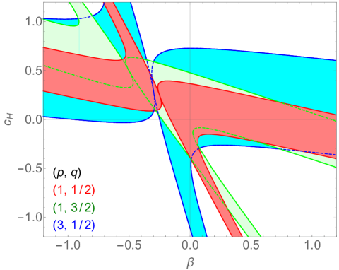
Figure 1: The allowed parameter region in the $\beta$-$c_{\rm H}$ plane obtained from the gravitational growth index in the shift-symmetric quadratic DHOST cosmology after GW170817. The parameters are given by $(p,q)=(1,1/2)$ (red), $(1,3)$ (green), and $(3,1/2)$ (blue). The first set of the parameters corresponds to the solution discussed in Crisostomi:2017pjs ; Crisostomi:2018bsp .

In this section, we investigate constraints on DHOST theories based on current observational limits on the gravitational growth index $\gamma$. For instance, clustering measurements from the BOSS DR12 give the limit as $\gamma=0.52\pm 0.10$ in Ref. Grieb:2016uuo (based on the analysis in Fourier space) and $\gamma=0.609\pm 0.079$ in Ref. Sanchez:2016sas (based on the analysis in configuration space). The constraints from BOSS DR14 are given as $\gamma=0.55\pm 0.19$ in Ref. Gil-Marin:2018cgo and $\gamma=0.580\pm 0.082$ in Ref. Zhao:2018jxv (by adding tomographic analysis). Since the typical value of the deviation from the central value of $\gamma$ in the current observations as shown above can be roughly estimated as $\lesssim{\cal O}(0.1)$, let us employ $\gamma=6/11\pm 0.1$ as a conservative constraint. For a given set of the model parameters $(p,q)$, this can be translated into constraints on $(\beta,c_{\rm H})$ using Eq. (63). The parameter regions in the $\beta$-$c_{\rm H}$ plane allowed by the constraint $\gamma=6/11\pm 0.1$ are plotted in Fig. 1 for $(p,q)=(1,1/2)$ (red), $(1,3/2)$ (green), and $(3,1/2)$ (blue). One finds from Fig. 1 that a constant-$\gamma$ curve for fixed $p$ and $q$ is a hyperbola in the $\beta$-$c_{\rm H}$ plane for $(p,q)$ and $\gamma$ that we are considering. This means that we have degeneracy between $c_{\rm H}$ and $\beta$ in the observations of the growth index. In contrast, in the GLPV theory we have $\beta=0$, and hence we can obtain for instance the following constraints on $c_{\rm H}$: $-0.4\leq c_{\rm H}\leq 0.4$ for $(p,q)=(1\,,1/2)$, $-0.4\leq c_{\rm H}\leq 0.5$ for $(1\,,3/2)$, and $-1.1\leq c_{\rm H}\leq 0.7$ for (3 ,1/2). Deriving the constraints for other values of $(p,q)$ is straightforward. It should be emphasized that the constraints we have obtained in Fig. 1 are those at high redshifts satisfying $\Omega_{\rm m}\simeq 1$.

To compare our results with previously known constraints, it is necessary to make further assumptions that connect the series expansion of $\alpha_{\rm H}$ and $\beta_{1}$ to their present values. Specifically, we assume that $\alpha_{\rm H}=c_{\rm H}\left(1-\Omega_{\rm m}\right)$, $\beta_{1}=\beta\left(1-\Omega_{\rm m}\right)$, and the leading order expression of $\gamma$ [Eq. (63)] are valid all the way up to the present time. Hereafter we focus on the specific parameter values $(p,q)=(1,1/2)$, which corresponds to the model discussed in Crisostomi:2017pjs ; Crisostomi:2018bsp , and demonstrate the allowed parameter region. Though details of constraints will be different for different choices of $(p,q)$, we expect that the order of the bounds is approximately the same.

Existing constraints on DHOST theories mainly come from the Newtonian stellar structure modified due to the partial breaking of the Vainshtein mechanism, which is characterized by a single parameter $\Upsilon_{1}:=-2(\alpha_{\rm H}+\beta_{1})^{2}/(\alpha_{\rm H}+2\beta_{1})$ (the definition here is for theories with $c_{\rm GW}^{2}=1$) Kobayashi:2014ida ; Langlois:2017dyl ; Dima:2017pwp . The lower bound on $\Upsilon_{1}$ has been obtained from the requirement that gravity is attractive at the stellar center: $\Upsilon_{1}>-2/3$ Saito:2015fza . The upper bound is given by comparing the minimum mass of stars with the hydrogen burning with the minimum mass of observed red dwarfs: $\Upsilon_{1}<1.6$ Sakstein:2015aac .

There are several attempts for improving the above bounds Jain:2015edg ; Babichev:2016jom ; Saltas:2018mxc , including the one concerning the speed of sound in the atmosphere of the Earth Babichev:2018rfj . Aside from the constraints from the Newtonian stellar structure, another constraint has been proposed, which comes from precise observations of the Hulse-Taylor pulsar. This can severely constrain the effective parameters through the coupling of gravitational waves to matter Jimenez:2015bwa ; Dima:2017pwp :$-7.5\times 10^{-3}\leq\alpha_{\rm H}+3\beta_{1}\leq 2.5\times 10^{-3}$. However, when deriving this result, several assumptions have been made and the resultant constraint would depend on the details of how the screening mechanism operates in a binary system. In this paper, we try to constrain the effective parameters without taking into account these potentially more stringent bounds, and use the most conservative constraint: $-2/3<\Upsilon_{1}<1.6$.

We plot in Fig. 2 the allowed parameter region in the $\beta$-$c_{\rm H}$ plane obtained from the constraints on the growth index (red) and stellar structure (black). As shown in Fig. 2, combining our results and the conservative constraints discussed above can break the degeneracy between $c_{\rm H}$ and $\beta$ without using the Halse-Taylor pulsar bound. The overlap region between these gives the constraints on both parameters: $-1.0\leq c_{\rm H}\leq 1.7$ and $-4.7\leq\beta\leq 1.8$.

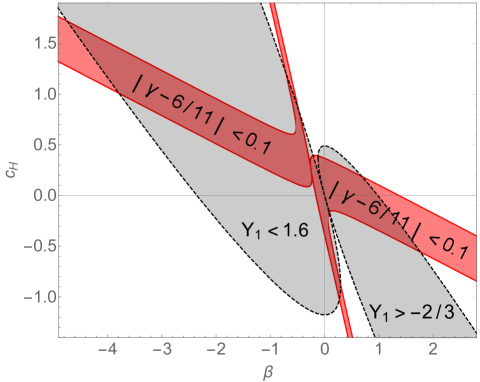
Figure 2: The allowed parameter region obtained from the gravitational growth index in the shift-symmetric quadratic DHOST cosmology after GW170817 is shown by the red area in the $\beta$-$c_{\rm H}$ plane. The parameters are given by $p=1,q=1/2$. For comparison, the existing constraints $-2/3\leq\Upsilon_{1}\leq 1.6$ Saito:2015fza ; Sakstein:2015aac are shown by the gray area.

Note that recently it was pointed out in Ref. Creminelli:2018xsv that the absence of gravitational wave decay into scalar modes requires $\alpha_{\rm H}+2\beta_{1}=0$. As seen from the fact that the denominator of $\Upsilon_{1}$ vanishes when this is satisfied, this is a special case which has not been explored so far. It would be interesting to investigate the behavior of gravity in this limiting case in detail, but it is beyond the scope of this paper, and we do not consider this constraint.

V Summary

In this paper, we have considered a possibility to constrain degenerate higher-order scalar-tensor (DHOST) theories by using the information about the linear growth of matter density fluctuations. In DHOST theories, the evolution equation for the linear matter density fluctuations is modified in such a way that the effective gravitational coupling is changed by the factor $\Xi_{\Phi}$ and the friction term has an additional contribution $\varsigma H$, both of which can be expressed in terms of the effective parameters $\alpha_{i}$ and $\beta_{i}$ used in the literature.

We have constructed cosmological models in DHOST theories as a series expansion in terms of $1-\Omega_{\rm m}$. In doing so, we have assumed for simplicity that cosmological solutions under consideration are attractors in shift-symmetric theories and subject to the tracker ansatz. The resultant cosmology is characterized by two model parameters $(p,q)$ and four independent effective parameters in general (i.e., six parameters in total), and upon imposing $c_{\rm GW}^{2}=1$ the number of independent parameters reduces to four in total. Our construction thus provides a concise description of DHOST cosmology during the matter dominated era and the early stage of the dark energy dominated era.

We have then explicitly expressed the gravitational growth index $\gamma$ in terms of $(p,q)$ and the effective parameters. We have found that the constant-$\gamma$ curve in the $\beta$-$c_{\rm H}$ plane generically is a hyperbola for $c_{\rm GW}^{2}=1$ and fixed $(p,q)$. One can thus obtain constraints on a certain combination of the effective parameters at high redshifts by using the observations of the growth index alone.

Under the additional assumption that our leading order results in $1-\Omega_{\rm m}$ expansion can be extrapolated all the way to the present time, we have compared the constraints from the growth index with the previously known bounds. Combining our results and the constraints from modifications of the gravitational law inside stellar objects, we have shown that the parameter degeneracy between $\alpha_{\rm H}/(1-\Omega_{\rm m})$ and $\beta_{1}/(1-\Omega_{\rm m})$ could be broken without using the Hulse-Taylor pulsar constraint, though our results slightly depend on the model parameters. Future-planned observations for large-scale structure would exclude the currently allowed region of the parameter space and serve as tests of the viability of DHOST theories.

Appendix A Explicit expressions for some coefficients

Let us write down explicitly the coefficients in Eqs. (33)–(34). The coefficients in Eq. (33) are given by

$$\nu_{Q}=\frac{3\Omega_{\rm m}}{2{\cal Z}}{\cal N}_{\Phi}\,,$$ (64)

$$\kappa_{Q}=\frac{3\Omega_{\rm m}}{8{\cal Z}}\biggl{\{}\Bigl{[}c_{1}+2\bigl{(}2\beta_{1}+\beta_{3}\bigr{)}\Bigr{]}{\cal F}_{\Phi}+\bigl{(}c_{2}-4\alpha_{\rm H}\bigr{)}{\cal F}_{\Psi}$$

$$\quad\quad\quad\quad\quad-\frac{M^{2}}{H}\biggl{[}2\bigl{(}2\beta_{1}+\beta_{3}\bigr{)}\frac{{\rm d}}{{\rm d}t}\left(\frac{{\cal F}_{\Phi}}{M^{2}}\right)-4\alpha_{\rm H}\frac{{\rm d}}{{\rm d}t}\left(\frac{{\cal F}_{\Psi}}{M^{2}}\right)\biggr{]}\biggr{\}}\,,$$ (65)

where we have defined the some dimensionless parameters as

$${\cal S}{\cal N}_{\Phi}=\alpha_{\rm H}\bigl{(}1+\alpha_{\rm H}\bigr{)}-\frac{1}{2}\bigl{(}1+\alpha_{\rm T}\bigr{)}\bigl{(}2\beta_{1}+\beta_{3}\bigr{)}\,,$$ (66)

$${\cal S}{\cal F}_{\Phi}=1+\alpha_{\rm T}\,,\ \ \ {\cal S}{\cal F}_{\Psi}=1+\alpha_{\rm H}\,,$$ (67)

$${\cal S}=\bigl{(}1+\alpha_{\rm H}\bigr{)}^{2}-\frac{1}{2}\bigl{(}1+\alpha_{\rm T}\bigr{)}\beta_{3}\,,$$ (68)

The denominator ${\cal Z}$ can be written as

$${\cal Z}=\frac{1}{4}\Biggl{\{}{\cal E}_{\Phi}c_{1}+{\cal E}_{\Psi}c_{2}-\biggl{[}b_{3}+\frac{2(2\beta_{1}+\beta_{3})}{H}\dot{\cal E}_{\Phi}-\frac{4\alpha_{\rm H}}{H}\dot{\cal E}_{\Psi}\biggr{]}\Biggr{\}}$$ (69)

where $c_{1}$, $c_{2}$, and $b_{3}$ were defined in Eqs (19), (20), and (28). We have also defined

$${\cal S}{\cal E}_{\Phi}=b_{1}\bigl{(}1+\alpha_{\rm T}\bigr{)}-b_{2}\bigl{(}1+\alpha_{\rm H}\bigr{)}\,,$$ (70)

$${\cal S}{\cal E}_{\Psi}=b_{1}\bigl{(}1+\alpha_{\rm H}\bigr{)}-\frac{1}{2}b_{2}\beta_{3}\,.$$ (71)

The coefficients in Eqs. (35) and (35) are

$$\mu_{a}={\cal N}_{a}\nu_{Q}\,,$$ (72)

$$\nu_{a}=-{\cal E}_{a}\nu_{Q}+{\cal N}_{a}\left[\kappa_{Q}+\frac{1}{a^{2}H^{2}}\frac{{\rm d}}{{\rm d}t}\left(a^{2}H\nu_{Q}\right)\right]\,,$$ (73)

$$\kappa_{a}=\frac{3}{2}\Omega_{\rm m}{\cal F}_{a}-{\cal E}_{a}\kappa_{Q}+\frac{{\cal N}_{a}}{a^{2}H^{3}}\frac{{\rm d}}{{\rm d}t}\left(a^{2}H^{2}\kappa_{Q}\right)\,,$$ (74)

for $a=\Psi\,,\Phi$, where

$${\cal S}{\cal N}_{\Psi}=-\bigl{(}1+\alpha_{\rm H}\bigr{)}\beta_{1}-\frac{1}{2}\beta_{3}\,.$$ (75)

The coefficients in Eq. (57) are given by

$$\varsigma^{(1)}=\frac{3}{Z}\left(c_{\rm H}+\beta\right)^{2}\bigl{(}c_{\rm M}-3w^{(0)}\bigr{)}\,,$$ (76)

$$\Xi^{(1)}_{\Phi}=c_{\rm T}+\frac{2}{Z}\Bigl{[}c_{\rm B}-c_{\rm M}+c_{\rm T}-\beta\bigl{(}c_{\rm M}-3w^{(0)}\bigr{)}\Bigr{]}^{2}$$

$$\quad\quad\quad-\frac{c_{\rm H}+\beta}{Z}\biggl{\{}6\bigl{(}1+w^{(0)}\bigr{)}+\bigl{(}c_{\rm M}-c_{\rm T}\bigr{)}\Bigl{[}1-2\bigl{(}c_{\rm M}-3w^{(0)}\bigr{)}\Bigr{]}$$

$$\quad\quad\quad\quad\quad\quad+\Bigl{[}c_{\rm B}-\beta\bigl{(}c_{\rm M}-3w^{(0)}\bigr{)}\Bigr{]}\Bigl{[}5-2\bigl{(}c_{\rm M}-3w^{(0)}\bigr{)}\Bigr{]}+3\bigl{(}c_{\rm H}+\beta\bigr{)}\bigl{(}c_{\rm M}-3w^{(0)}\bigr{)}\biggr{\}}\,,$$ (77)

where

$$Z=3\bigl{(}1+w^{(0)}\bigr{)}+2c_{\rm M}+\Bigl{[}1-2\bigl{(}c_{\rm M}-3w^{(0)}\bigr{)}\Bigr{]}\Bigl{[}c_{\rm B}-c_{\rm H}-\beta\bigl{(}c_{\rm M}-3w^{(0)}+1\bigr{)}\Bigr{]}\,.$$ (78)

We can then finally obtain the explicit expression $\gamma$ in the main text by sustituting Eqs. (76) and (77) into Eq. (60).

References

- (1) A. G. Riess et al. [Supernova Search Team], “Observational evidence from supernovae for an accelerating universe and a cosmological constant,” Astron. J. 116 (1998) 1009 [astro-ph/9805201].
- (2) S. Perlmutter et al. [Supernova Cosmology Project Collaboration], “Measurements of Omega and Lambda from 42 high redshift supernovae,” Astrophys. J. 517 (1999) 565 [astro-ph/9812133].
- (3) M. Ostrogradsky, Mem. Ac. St. Petersbourg VI 4 (1850) 385.
- (4) R. P. Woodard, “Ostrogradsky’s theorem on Hamiltonian instability,” Scholarpedia 10, no. 8, 32243 (2015) [arXiv:1506.02210 [hep-th]].
- (5) D. Langlois and K. Noui, “Degenerate higher derivative theories beyond Horndeski: evading the Ostrogradski instability,” JCAP 1602 (2016) no.02, 034 [arXiv:1510.06930 [gr-qc]].
- (6) M. Crisostomi, K. Koyama and G. Tasinato, “Extended Scalar-Tensor Theories of Gravity,” JCAP 1604 (2016) no.04, 044 [arXiv:1602.03119 [hep-th]].
- (7) J. Ben Achour, D. Langlois and K. Noui, “Degenerate higher order scalar-tensor theories beyond Horndeski and disformal transformations,” Phys. Rev. D 93 (2016) no.12, 124005 [arXiv:1602.08398 [gr-qc]].
- (8) J. Ben Achour, M. Crisostomi, K. Koyama, D. Langlois, K. Noui and G. Tasinato, “Degenerate higher order scalar-tensor theories beyond Horndeski up to cubic order,” JHEP 1612 (2016) 100 [arXiv:1608.08135 [hep-th]].
- (9) D. Langlois, “Degenerate Higher-Order Scalar-Tensor (DHOST) theories,” arXiv:1707.03625 [gr-qc].
- (10) D. Langlois, “Dark Energy and Modified Gravity in Degenerate Higher-Order Scalar-Tensor (DHOST) theories: a review,” arXiv:1811.06271 [gr-qc].
- (11) T. Kobayashi, “Horndeski theory and beyond: a review,” arXiv:1901.07183 [gr-qc].
- (12) G. W. Horndeski, “Second-order scalar-tensor field equations in a four-dimensional space,” Int. J. Theor. Phys. 10, 363 (1974).
- (13) C. Deffayet, X. Gao, D. A. Steer and G. Zahariade, “From k-essence to generalised Galileons,” Phys. Rev. D 84, 064039 (2011) [arXiv:1103.3260 [hep-th]].
- (14) T. Kobayashi, M. Yamaguchi and J. Yokoyama, “Generalized G-inflation: Inflation with the most general second-order field equations,” Prog. Theor. Phys. 126 (2011) 511 [arXiv:1105.5723 [hep-th]].
- (15) M. Zumalacrregui and J. Garca-Bellido, “Transforming gravity: from derivative couplings to matter to second-order scalar-tensor theories beyond the Horndeski Lagrangian,” Phys. Rev. D 89 (2014) 064046 [arXiv:1308.4685 [gr-qc]].
- (16) J. Gleyzes, D. Langlois, F. Piazza and F. Vernizzi, “Healthy theories beyond Horndeski,” Phys. Rev. Lett. 114 (2015) no.21, 211101 [arXiv:1404.6495 [hep-th]].
- (17) J. Gleyzes, D. Langlois, F. Piazza and F. Vernizzi, “Exploring gravitational theories beyond Horndeski,” JCAP 1502 (2015) 018 [arXiv:1408.1952 [astro-ph.CO]].
- (18) B. P. Abbott et al. [LIGO Scientific and Virgo Collaborations], “GW170817: Observation of Gravitational Waves from a Binary Neutron Star Inspiral,” Phys. Rev. Lett. 119, no. 16, 161101 (2017) [arXiv:1710.05832 [gr-qc]].
- (19) B. P. Abbott et al. [LIGO Scientific and Virgo and Fermi-GBM and INTEGRAL Collaborations], “Gravitational Waves and Gamma-rays from a Binary Neutron Star Merger: GW170817 and GRB 170817A,” Astrophys. J. 848, no. 2, L13 (2017) [arXiv:1710.05834 [astro-ph.HE]].
- (20) L. Lombriser and A. Taylor, “Breaking a Dark Degeneracy with Gravitational Waves,” JCAP 1603 (2016) no.03, 031 [arXiv:1509.08458 [astro-ph.CO]].
- (21) L. Lombriser and N. A. Lima, “Challenges to Self-Acceleration in Modified Gravity from Gravitational Waves and Large-Scale Structure,” Phys. Lett. B 765 (2017) 382 [arXiv:1602.07670 [astro-ph.CO]].
- (22) P. Creminelli and F. Vernizzi, “Dark Energy after GW170817 and GRB170817A,” Phys. Rev. Lett. 119, no. 25, 251302 (2017) [arXiv:1710.05877 [astro-ph.CO]].
- (23) J. Sakstein and B. Jain, “Implications of the Neutron Star Merger GW170817 for Cosmological Scalar-Tensor Theories,” Phys. Rev. Lett. 119, no. 25, 251303 (2017) [arXiv:1710.05893 [astro-ph.CO]].
- (24) J. M. Ezquiaga and M. Zumalacrregui, “Dark Energy After GW170817: Dead Ends and the Road Ahead,” Phys. Rev. Lett. 119, no. 25, 251304 (2017) [arXiv:1710.05901 [astro-ph.CO]].
- (25) T. Baker, E. Bellini, P. G. Ferreira, M. Lagos, J. Noller and I. Sawicki, “Strong constraints on cosmological gravity from GW170817 and GRB 170817A,” Phys. Rev. Lett. 119, no. 25, 251301 (2017) [arXiv:1710.06394 [astro-ph.CO]].
- (26) D. Langlois, R. Saito, D. Yamauchi and K. Noui, “Scalar-tensor theories and modified gravity in the wake of GW170817,” Phys. Rev. D 97, no. 6, 061501 (2018) [arXiv:1711.07403 [gr-qc]].
- (27) T. Kobayashi, Y. Watanabe and D. Yamauchi, “Breaking of Vainshtein screening in scalar-tensor theories beyond Horndeski,” Phys. Rev. D 91 (2015) no.6, 064013 [arXiv:1411.4130 [gr-qc]].
- (28) M. Crisostomi and K. Koyama, “Vainshtein mechanism after GW170817,” Phys. Rev. D 97, no. 2, 021301 (2018) [arXiv:1711.06661 [astro-ph.CO]].
- (29) A. Dima and F. Vernizzi, “Vainshtein Screening in Scalar-Tensor Theories before and after GW170817: Constraints on Theories beyond Horndeski,” Phys. Rev. D 97, no. 10, 101302 (2018) [arXiv:1712.04731 [gr-qc]].
- (30) R. Saito, D. Yamauchi, S. Mizuno, J. Gleyzes and D. Langlois, “Modified gravity inside astrophysical bodies,” JCAP 1506 (2015) 008 [arXiv:1503.01448 [gr-qc]].
- (31) J. Sakstein, “Testing Gravity Using Dwarf Stars,” Phys. Rev. D 92 (2015) 124045 [arXiv:1511.01685 [astro-ph.CO]].
- (32) R. K. Jain, C. Kouvaris and N. G. Nielsen, “White Dwarf Critical Tests for Modified Gravity,” Phys. Rev. Lett. 116 (2016) no.15, 151103 [arXiv:1512.05946 [astro-ph.CO]].
- (33) E. Babichev, K. Koyama, D. Langlois, R. Saito and J. Sakstein, “Relativistic Stars in Beyond Horndeski Theories,” Class. Quant. Grav. 33 (2016) no.23, 235014 [arXiv:1606.06627 [gr-qc]].
- (34) I. D. Saltas, I. Sawicki and I. Lopes, “White dwarfs and revelations,” JCAP 1805 (2018) no.05, 028 [arXiv:1803.00541 [astro-ph.CO]].
- (35) E. Babichev and A. Lehbel, “The sound of DHOST,” arXiv:1810.09997 [gr-qc].
- (36) L. M. Wang and P. J. Steinhardt, “Cluster abundance constraints on quintessence models,” Astrophys. J. 508 (1998) 483 [astro-ph/9804015].
- (37) C. de Rham and A. Matas, “Ostrogradsky in Theories with Multiple Fields,” JCAP 1606 (2016) no.06, 041 [arXiv:1604.08638 [hep-th]].
- (38) D. Langlois, M. Mancarella, K. Noui and F. Vernizzi, “Effective Description of Higher-Order Scalar-Tensor Theories,” JCAP 1705 (2017) no.05, 033 [arXiv:1703.03797 [hep-th]].
- (39) C. de Rham and S. Melville, “Gravitational Rainbows: LIGO and Dark Energy at its Cutoff,” Phys. Rev. Lett. 121 (2018) no.22, 221101 [arXiv:1806.09417 [hep-th]].
- (40) M. Crisostomi and K. Koyama, “Self-accelerating universe in scalar-tensor theories after GW170817,” arXiv:1712.06556 [astro-ph.CO].
- (41) M. Crisostomi, K. Koyama, D. Langlois, K. Noui and D. A. Steer, “Cosmological evolution in DHOST theories,” arXiv:1810.12070 [hep-th].
- (42) S. Hirano, T. Kobayashi, H. Tashiro and S. Yokoyama, “Matter bispectrum beyond Horndeski theories,” Phys. Rev. D 97, no. 10, 103517 (2018) [arXiv:1801.07885 [astro-ph.CO]].
- (43) G. D’Amico, Z. Huang, M. Mancarella and F. Vernizzi, “Weakening Gravity on Redshift-Survey Scales with Kinetic Matter Mixing,” JCAP 1702 (2017) 014 [arXiv:1609.01272 [astro-ph.CO]].
- (44) A. De Felice, T. Kobayashi and S. Tsujikawa, “Effective gravitational couplings for cosmological perturbations in the most general scalar-tensor theories with second-order field equations,” Phys. Lett. B 706 (2011) 123 [arXiv:1108.4242 [gr-qc]].
- (45) A. De Felice and S. Tsujikawa, “Conditions for the cosmological viability of the most general scalar-tensor theories and their applications to extended Galileon dark energy models,” JCAP 1202 (2012) 007 [arXiv:1110.3878 [gr-qc]].
- (46) A. De Felice and S. Tsujikawa, “Cosmological constraints on extended Galileon models,” JCAP 1203 (2012) 025 [arXiv:1112.1774 [astro-ph.CO]].
- (47) N. Frusciante, R. Kase, K. Koyama, S. Tsujikawa and D. Vernieri, “Tracker and scaling solutions in DHOST theories,” Phys. Lett. B 790, 167 (2019) [arXiv:1812.05204 [gr-qc]].
- (48) D. Yamauchi, S. Yokoyama and H. Tashiro, “Constraining modified theories of gravity with the galaxy bispectrum,” Phys. Rev. D 96 (2017) no.12, 123516 [arXiv:1709.03243 [astro-ph.CO]].
- (49) J. N. Grieb et al. [BOSS Collaboration], “The clustering of galaxies in the completed SDSS-III Baryon Oscillation Spectroscopic Survey: Cosmological implications of the Fourier space wedges of the final sample,” Mon. Not. Roy. Astron. Soc. 467, no. 2, 2085 (2017) [arXiv:1607.03143 [astro-ph.CO]]
- (50) A. G. Sanchez et al. [BOSS Collaboration], “The clustering of galaxies in the completed SDSS-III Baryon Oscillation Spectroscopic Survey: cosmological implications of the configuration-space clustering wedges,” Mon. Not. Roy. Astron. Soc. 464, no. 2, 1640 (2017) [arXiv:1607.03147 [astro-ph.CO]].
- (51) H. Gil-Marn et al., “The clustering of the SDSS-IV extended Baryon Oscillation Spectroscopic Survey DR14 quasar sample: structure growth rate measurement from the anisotropic quasar power spectrum in the redshift range ,” Mon. Not. Roy. Astron. Soc. 477, no. 2, 1604 (2018)
- (52) G. B. Zhao et al., “The clustering of the SDSS-IV extended Baryon Oscillation Spectroscopic Survey DR14 quasar sample: a tomographic measurement of cosmic structure growth and expansion rate based on optimal redshift weights,” arXiv:1801.03043 [astro-ph.CO].
- (53) J. Beltran Jimenez, F. Piazza and H. Velten, “Evading the Vainshtein Mechanism with Anomalous Gravitational Wave Speed: Constraints on Modified Gravity from Binary Pulsars,” Phys. Rev. Lett. 116 (2016) no.6, 061101 [arXiv:1507.05047 [gr-qc]].
- (54) P. Creminelli, M. Lewandowski, G. Tambalo and F. Vernizzi, “Gravitational Wave Decay into Dark Energy,” JCAP 1812, no. 12, 025 (2018) [arXiv:1809.03484 [astro-ph.CO]].