The Extremely High Dark Matter Halo Concentration of the
Relic Compact Elliptical Galaxy Mrk 1216

Abstract

Spatially compact stellar profiles and old stellar populations have established compact elliptical galaxies (CEGs) as local analogs of the high-redshift “red nuggets” thought to represent the progenitors of today’s early-type galaxies (ETGs). To address whether the structure of the dark matter (DM) halo in a CEG also reflects the extremely quiescent and isolated evolution of its stars, we use a new $\approx 122$ ks Chandra observation together with a shallow $\approx 13$ ks archival observation of the CEG Mrk 1216 to perform a hydrostatic equilibrium analysis of the luminous and relaxed X-ray plasma emission extending out to a radius $0.85{r_{2500}}$. We examine several DM model profiles and in every case obtain a halo concentration $(c_{200})$ that is a large positive outlier in the theoretical $\Lambda$CDM $c_{200}-M_{200}$ relation; i.e., ranging from $3.4\,\sigma-6.3\,\sigma$ above the median $\Lambda$CDM relation in terms of the intrinsic scatter. The high value of $c_{200}$ we measure implies an unusually early formation time that firmly establishes the relic nature of the DM halo in Mrk 1216. The highly concentrated DM halo leads to a higher DM fraction and smaller total mass slope at $1R_{e}$ compared to nearby normal ETGs. In addition, the highly concentrated total mass profile of Mrk 1216 cannot be described by MOND without adding DM, and it deviates substantially from the Radial Acceleration Relation. Our analysis of the hot plasma indicates the halo of Mrk 1216 contains $\approx 80\%$ of the cosmic baryon fraction within ${r_{200}}$. The radial profile of the ratio of cooling time to free-fall time varies within a narrow range $({t_{\rm c}}/{t_{\rm ff}}\approx 14-19)$ over a large central region ($r\leq 10$ kpc) suggesting “precipitation-regulated AGN feedback” for a multiphase plasma, though presently there is little evidence for cool gas in Mrk 1216. Finally, other than its compact stellar size, the stellar, gas, and DM properties of Mrk 1216 are remarkably similar to those of the nearby fossil group NGC 6482.

1. Introduction

Massive early-type galaxies (ETGs) are widely believed to have formed in a two-phase process (e.g., Oser et al. 2010). Phase 1 occurs at early times $(z\gtrsim 2)$ when dissipative gas infall leads to rapid star formation and, along with some dark matter (DM) halo contraction (e.g., Dutton et al. 2015), produces a very compact “red nugget.” Subsequent evolution in Phase 2 is primarily non-dissipative driven by collisionless (“dry”) mergers, the effect of which is mostly accretive (i.e., increasing the size of the stellar halo) with little or no star formation. This later slow accretive phase is revealed by the stellar mass-size evolution of ETGs (e.g., Daddi et al. 2005; van Dokkum et al. 2008; Damjanov et al. 2011; van der Wel et al. 2014) and through multi-component decompositions of nearby ETGs (Huang et al. 2013). To study the end of Phase 1 requires mapping the radial mass profiles of galaxies at $z\sim 2$. Unfortunately, even with stellar dynamics detailed mass mapping is not possible at present since only an average velocity dispersion within approximately the stellar half-light radius $(R_{e})$ can be measured for $z\sim 2$ galaxies (e.g., Toft et al. 2012; Rhoads et al. 2014; Longhetti et al. 2014; van de Sande et al. 2014).

With detailed mass mapping of red nuggets extremely challenging, an alternative approach is to study local analogs (e.g., van den Bosch et al. 2012; Trujillo et al. 2014). van den Bosch et al. (2015) conducted a local survey of galaxies based on (among other criteria) the estimated size of the gravitational radius of influence of the central super-massive black hole (SMBH). From this survey they identified a sample of compact elliptical galaxies (CEGs) that have remarkable properties (Yıldırım et al. 2017, hereafter Y17, and references therein). (1) They have very old ($\gtrsim 13$ Gyr) stellar populations (e.g., Y17; Ferré-Mateu et al. 2017). (2) They have compact stellar surface brightness profiles that obey the stellar mass-size relationship for $z\sim 2$ galaxies instead of $z=0$. (3) Some of the CEGs have evidence for over-massive SMBHs with respect to the ${M_{\rm BH}-\sigma}$ relation (e.g., Ferré-Mateu et al. 2015; Yıldırım et al. 2015; Walsh et al. 2015, 2017, see also Savorgnan & Graham 2016). Properties (1) and (2) suggest that these CEGs are ancient relic galaxies that have skipped the “Phase 2” of slow accretion of an extended stellar envelope. In other words, they are likely passively evolved direct descendants of the high-redshift red nugget population, and therefore provide a new and more accessible avenue for studying the detailed structure of red nuggets.

It is presently unknown whether the DM profiles corroborate the interpretation of CEGs as relic galaxies. The scatter about the median $\Lambda$CDM $c_{200}-M_{200}$ relation reflects the halo formation time, history, and environment (e.g., Bullock et al. 2001; Neto et al. 2007; Ludlow et al. 2016; Ragagnin et al. 2018). Consequently, if the CEGs are truly red nugget analogs, their halo concentrations should reflect the early formation epoch and isolated evolution and thus appear as large, positive outliers in the local $c_{200}-M_{200}$ relation.

Motivated primarily by the desire to map the gravitating mass profiles of CEGs, in Buote & Barth (2018, hereafter Paper 1) we described the results of the first systematic search for extended, luminous X-ray emission in CEGs suitable for detailed hydrostatic equilibrium (HE) analysis of their mass profiles. Of the 16 CEGs studied by Y17, we identified two objects – Mrk 1216 and PGC 032873 – that are extremely promising for X-ray study and presented initial constraints on their mass profiles (see also Werner et al. 2018). Only for Mrk 1216 were the existing Chandra Cycle 16 data of sufficient quality for a detailed HE mass analysis from which we obtained the first tentative evidence for an above average halo concentration for a CEG. We also placed a tentative constraint on the SMBH mass consistent with the large (“over-massive”) value obtained from stellar dynamics by Walsh et al. (2017).

To confirm and strengthen these initial results, we submitted a Chandra proposal for a deep 130 ks observation of Mrk 1216 which was approved and allocated time in Cycle 19. Here we report a detailed analysis of the Cycle 19 image and spectra in conjunction with an updated analysis of the shallow archival Cycle 16 data studied in Paper 1. Some properties of Mrk 1216 are listed in Table 1.

The paper is organized as follows. We describe the Chandra X-ray observations and the data preparation in §2. In §3 we perform a detailed analysis of the image morphology to search for features associated with AGN feedback. In §4 we describe the spectral analysis. We define the spectral model in §4.1 and present the results of the spectral fitting in §4.2. We present the HE models in §5, the fitting methodology in §6, the results of the HE mass analysis in §7, and the error budget in §8. We discuss several topics in §9 and present our conclusions in §10.

2. Observations and Data Preparation

Table 1Target Properties

		Distance	Scale	$N_{\rm H}$	$L_{\rm H}$	$R_{e}$	$\sigma_{e}$	$L_{\rm x}$	${k_{\rm B}T}$
Name	Redshift	(Mpc)	(kpc/arcsec)	($10^{20}$ cm-2)	$(10^{11}\,L_{\odot})$	(kpc)	(km/s)	($10^{42}$ ergs s-1)	(keV)
Mrk 1216	0.021328	97.0	0.45	4.0	1.14	2.3	308	$1.7\pm 0.1$	$0.73\pm 0.01$

Table 2Observations

					Exposure
Cycle	Obs. ID	Obs. Date	Instrument	Active CCDs	(ks)
16	17061	2015 Jun. 12	ACIS-S	S1,S2,S3,S4	12.9
19	20342	2018 Jan. 9	ACIS-S	I2,I3,S2,S3	31.7
19	20924	2018 Jan. 9	ACIS-S	I2,I3,S2,S3	29.7
19	20925	2018 Jan. 12	ACIS-S	I2,I3,S2,S3	31.4
19	20926	2018 Jan. 14	ACIS-S	I2,I3,S2,S3	29.7

We list the details of the Chandra observations in Table 2. In Cycle 19 Mrk 1216 was observed with the ACIS CCDs during 2018 from January 9 to January 14 in four exposures for $\sim 30$ ks each. The aim point of the telescope was located on the S3 chip (i.e., ACIS-S configuration), although a non-standard chip set was used (notably with the I2 and I3 chips both active) to allow for a simultaneous measurement of the background. We prepared the data for imaging and spectral analysis using the CIAO (v4.10) and HEASOFT (v6.24) software suites along with version 4.8.1 of the Chandra calibration database.

We begin by reprocessing each each Cycle 19 exposure with the latest calibration information. To clean these exposures of periods of high particle background, we created broad-band light curves extracted from regions without obvious point sources and excluding most of the emission from Mrk 1216. We filtered the light curves with a $3\sigma$ clip procedure (see CIAO deflare and lc_clean tasks) which resulted in almost no time removed for a combined total exposure of 122.4 ks. The cleaned times for each exposure are listed in Table 2.

To generate images for the entire Cycle 19 data set, we first combine the individual events lists into a single file. We begin by correcting the absolute astrometry for each exposure using the ciao task reproject_aspect along with initial point source lists obtained from their 0.5-7.0 keV images using the ciao task wavdetect. We combined the aligned exposure into a single events list from which an image and exposure map was created using the ciao task merge_obs. In this way we create merged images of the entire Cycle 19 observation of varying energy ranges and pixel sizes.

Since our focus is on the diffuse emission, we generate a source list using wavdetect applied to the $0.5-7.0$ keV image. We verify the detected point sources by visual inspection while excluding the detection of the center of Mrk 1216. We assign a radius for each source to correspond to the 95% encircled energy fraction for a 1-keV monochromatic point source appropriate for its off-axis location in the ACIS field.

While most of our imaging and spectral analysis employs a local background measured directly from the Chandra observations of Mrk 1216, we nevertheless, as described below, make some use of the background derived instead from regions of nominally blank sky. For each of the Cycle 19 observations we created such “blank sky” images using the ciao tasks blanksky an blanksky_image. We co-add the images of each exposure to obtain a total blank-sky background image matching the energy band and spatial binning for the corresponding source image.

For our primary spectral analysis, we defined a series of concentric, circular annuli positioned very near to the optical center (§3) while masking out point sources, chip gaps, and other off-chip regions. There is significant latitude in choosing the widths of the annuli depending on the scientific objectives. We balanced the need for source counts with the need to sample the radial profile within $1R_{e}$ arriving at a criterion of $\approx 1000$ background-subtracted counts in the $0.5-2.0$ keV image (using the softer band to emphasize the ${k_{\rm B}T}=0.5-1$ keV hot plasma contribution). In addition, to better probe the gravitational effect of a central SMBH, we required the central aperture to have a radius of 2 pixels ($0.982\arcsec$ radius), enclosing $\approx 90\%$ of the point spread function, and containing a little below 600 source counts. The annulus definitions are listed in Table 6. Note that all the annuli listed in Table 6 lie entirely on the S3 chip except annulus 10 for which almost 30% of the area lies on the S2 chip. Finally, to constrain the local background, we also included a single large annulus ($R=4.1\arcmin-14.8\arcmin$, not listed in Table 6) with negligible source counts but containing most of the available area of the S2, I2, and I3 chips.

We extracted a spectrum and created counts-weighted redistribution matrix (RMF) and auxiliary response (ARF) files using the ciao task specextract for each region and Cycle 19 exposure. Then for each region we created a combined spectrum, RMF, and ARF files using the ciao task combine_spectra. Combining the RMFs and ARFs in this way is a convenience and should be appropriate for Mrk 1216 since constraints on the spectral models are dominated by statistical rather than systematic errors in the response. Nevertheless, to verify this expectation we have also analyzed the un-merged spectra (§4.2 and Appendix A).

We also examined whether enhanced Solar Wind Charge Exchange (SWCX) emission may have significantly affected the Cycle 19 observations. We used the Level 2 data from SWEPAM to obtain the solar proton flux during each Chandra observation. All 4 Cycle 19 exposures have solar proton flux below $\approx 2\times 10^{8}$ cm^-2 s^-1 indicating significant proton flare contamination is not expected (Fujimoto et al. 2007).

Finally, we have updated and prepared the Cycle 16 observation as above, but without merging it with the Cycle 19 data, and maintaining the same annuli definitions used in Paper 1.

3. Image Morphology: Search for Structural Evidence of AGN Feedback

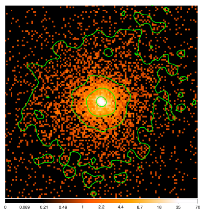
Figure 1.— 0.5-2.0 keV raw image of the central $1\arcmin\times 1\arcmin$ region with smoothed, logarithmically spaced contours overlaid. The bottom color bar shows the counts per pixel, where 1 pixel is $0.492\arcsec\times 0.492\arcsec$.

Table 3Ellipticity Profile of the Central 10 kpc

$a$	$a$	$\epsilon$	PA
(arcsec)	(kpc)		(deg N-E)
1.23	0.55	$0.20\pm 0.08$	$66\pm 45$
3.69	1.66	$0.22\pm 0.06$	$67\pm 30$
6.15	2.77	$0.06\pm 0.03$	$93\pm 26$
8.61	3.88	$0.09\pm 0.03$	$87\pm 12$
11.32	5.09	$0.07\pm 0.03$	$83\pm 20$
14.27	6.42	$0.05\pm 0.03$	$98\pm 28$
17.96	8.08	$0.04\pm 0.03$	$110\pm 28$
22.39	10.07	$0.05\pm 0.02$	$106\pm 22$

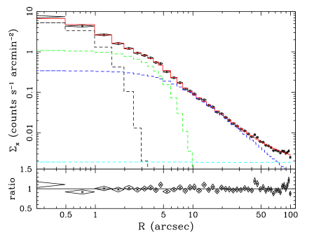
Figure 2.— 0.5-2.0 keV surface brightness profile and best-fitting model (Table 4) of the central $\sim 100\arcsec$. The model is fully two-dimensional but has been binned radially for display purposes only ($\sim 200$ counts per bin). The total model is shown by the solid red bins. The individual model components are as follows: gauss 1 (dashed black), gauss 2 (dashed green), beta (dashed blue), and constant background (dashed cyan). The bottom panel shows the data/model ratio.

Table 4Surface Brightness Model Parameters

	$A$	FWHM		PA	$r_{c}$
Model	(cts s-1 arcmin-2)	(arcsec)	$\epsilon$	(deg N-E)	(arcsec)	$\beta$
gauss 1	$6.01_{-0.41}^{+0.44}$	$2.07_{-0.12}^{+0.13}$	$0.29_{-0.05}^{+0.05}$	$50_{-6}^{+6}$	$\cdots$	$\cdots$
gauss 2	$1.09_{-0.12}^{+0.11}$	$6.75_{-0.29}^{+0.34}$	$0.09_{-0.04}^{+0.04}$	$92_{-14}^{+14}$	$\cdots$	$\cdots$
beta	$0.34_{-0.10}^{+0.13}$	$\cdots$	$0$	$\cdots$	$6.2_{-1.3}^{+2.0}$	$0.52_{-0.02}^{+0.03}$
const bkg	$0.0019_{-0.0002}^{+0.0002}$	$\cdots$	$\cdots$	$\cdots$	$\cdots$	$\cdots$

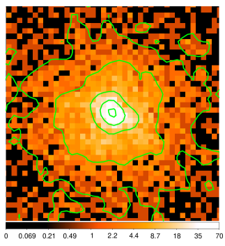
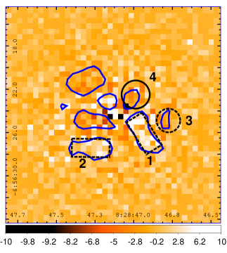
Figure 3.— Residual image analysis. (Left Panel) 0.5-2.0 keV image of the central $20\arcsec\times 20\arcsec$ region. The contours are different from those displayed in Fig. 1 and use square-root spacing. In addition, this image has the point sources filled in with local background (§3). (Right Panel) Residual image created by subtracting the smooth multi-component surface-brightness model (Table 4 and Fig. 2). The smoothed contours are displayed with linear spacing. The black regions (dashed and solid) are those showing the most significant fluctuations with respect to their local environment (§3).

Table 5Residual Map Region Properties

	Center		Counts			Ratio	sign(Ratio)$\sqrt{\rm|Ratio|}$
Region	RA	Dec	Image	Model	Residual	(%)	(%)
1	8:28:46.950	$-$6:56:26.092	239	175.5	$+63.5$	$+36.2\pm 8.8$	$+16.7\pm 4.3$
2	8:28:47.282	$-$6:56:27.420	143	108.1	$+34.9$	$+32.2\pm 11.1$	$+15.0\pm 5.4$
3	8:28:46.799	$-$6:56:24.885	36	57.1	$-21.1$	$-36.9_{-10.5}^{+12.3}$	$-20.6_{-5.1}^{+6.0}$
4	8:28:47.002	$-$6:56:22.486	147	169.3	$-22.3$	$-13.2\pm 7.1$	$-6.8\pm 3.5$

Since the demise of the classical cooling flow paradigm brought about by early observations with the Chandra and XMM-Newton telescopes (e.g., Peterson & Fabian 2006), it is now generally accepted that in the central regions of cool-core clusters and isolated massive galaxies episodic AGN feedback suppresses and regulates gas cooling (e.g., McNamara & Nulsen 2007). Although the details of the feedback process are complex and are the subject of much current research in the field, the fundamental mechanism by which the AGN energizes the hot plasma is widely believed to be mechanical feedback from AGN radio jets; i.e, the jet interacts with the hot plasma and, e.g., inflates bubbles and cavities, generates weak shocks and sound waves, which deliver energy to the hot plasma. Consequently, in this section we have performed a detailed search for signs of AGN feedback in Mrk 1216 in the form of irregular features in the central part of the X-ray image. (Spectral signatures are examined in §4.2.3 and §4.2.4). Since radio observations of Mrk 1216 currently indicate only a weak point source (limited to the single $9.2\pm 0.2$ mJy detection in the 1.4 GHz NVSS, Condon et al. 1998), our present investigation of signs of AGN feedback will consider mainly the X-ray image morphology. We focus our analysis on the Cycle 19 data since the Cycle 16 data do not provide strong constraints on the central image structure (Paper 1).

We focus our analysis on the merged Cycle 19 image in the $0.5-2.0$ keV band using a monochromatic 1-keV exposure map. In Figure 1 we show the raw image of the central $1\arcmin\times 1\arcmin$ region at full resolution overlaid with smooth contours. The image appears very regular with rather round (though noisy) contours; i.e. the impact of AGN feedback on the image of Mrk 1216 is not dramatic in the same way as observed for some well-studied Virgo galaxies – M84 (Finoguenov et al. 2008) and NGC 4636 (Baldi et al. 2009). It is possible, however, that features similar to those seen in some Virgo galaxies are present in Mrk 1216 but are merely less prominent owing to Mrk 1216 being 5-6 times more distant than Virgo. Therefore, a quantitative assessment of image morphology is required.

3.1. Moment Analysis

To make a quantitative analysis of the X-ray image morphology, we begin by computing the ellipticity $(\epsilon)$, position angle (PA), and centroid evaluated within elliptical apertures as a function of semi-major axis $a$. We apply an iterative scheme equivalent to diagonalizing the moment of inertia tensor of the image region (Carter & Metcalfe 1980; see Buote & Canizares 1994 for application to X-ray images of elliptical galaxies). Before applying this technique, we replaced detected point sources (§2) with local background using the CIAO dmfilth tool.

In Table 3 we list the ellipticity and position angle as a function of $a$ within 10 kpc ($\approx 22\arcsec$). Not listed in the table is the center position which is quite steady; e.g., the center shifts by only $1.1\pm 0.4$ pixels ($0.5\arcsec\pm 0.2\arcsec$) when comparing the centroids of the $a=1.23\arcsec,22.39\arcsec$ apertures. Within the relatively large statistical errors, the PA within $\approx 10$ kpc is consistent with the $H$-band value of $70.15^{\circ}$ reported by Y17, with some weak evidence it increases near $a=10$ kpc (also see below). The ellipticity, however, displays a clear radial variation. Within $a\approx 4\arcsec$ the image is modestly flattened with $\epsilon\approx 0.20$. The ellipticity then drops quickly for larger $a$ to a small value $\approx 0.05$ not inconsistent with $\epsilon=0$. The X-ray morphology is thus broadly similar to that observed for the relaxed, fossil-like elliptical galaxy NGC 720 (e.g., Buote et al. 2002); i.e., within $\approx 1R_{e}$ the X-ray image is moderately flattened (though rounder than the stellar isophotes, $\epsilon=0.42$ – Y17) and consistent with being aligned with the stellar image before giving way to a much rounder X-ray image at larger radius. Hence, the moment analysis of the centroid, $\epsilon$, and PA within $a\approx 10$ kpc does not indicate the presence of irregular surface brightness features.

3.2. Two-Dimensional Model

To search for more subtle features in the X-ray image we construct a smooth two-dimensional model, subtract it from the image, and inspect the residual image using the sherpa fitting package within ciao. We initially defined a model consisting of an isothermal $\beta$ model (Cavaliere & Fusco-Femiano 1978) for the hot gas and a constant background. Each model component was folded through the exposure map and fitted (using the C-statistic) to the full-resolution image within a radius of $\approx 100\arcsec$ from the center of the galaxy (close to the edge of the S3). For our fiducial analysis here and throughout the paper, we defined the center of the X-ray image to be the centroid computed within a circular aperture of radius $3\arcsec$ initially located at the emission peak. This gives $\rm(R.A.,Dec)$ of (8:28:47.1410, $-$6:56:24.368) which is very consistent with the stellar center determined by Springob et al. (2014), though we note that there are $1\arcsec$-level differences in the various position references collected by NED. (We examine the effect of choosing a slightly different center in §8.1.)

We found that the initial model fit produced significant residuals within central region. We noticed a substantial reduction in these residuals upon adding two gaussian components with different widths; i.e., a crude multi-gauss expansion. (Adding more gaussian components produced comparatively minor changes.) The best-fitting parameters and $1\sigma$ errors are listed in Table 4. In Figure 2 we plot the best-fitting two-dimensional model (and data/model ratio) binned as a radial profile where each bin contains $\sim 200$ counts. Notice in particular the negligible residuals within the central region. The gaussian components display $\epsilon$ and PA values similar to the moment analysis (Table 3); i.e., PA values broadly consistent with the $H$-band value with a moderately flattened $\epsilon\approx 0.30$ that drops to a much smaller value ($\epsilon\approx 0.10$) indicating nearly round isophotes at larger radius. (We emphasize that the individual components of our surface brightness model – $\beta$ model and two gaussians – should not be thought about as distinct physically meaningful mass components. We describe the physical model(s) later; i.e., the fiducial HE model in Table 8.)

When $\epsilon$ is allowed to vary for the $\beta$ model, we obtain values $\epsilon\approx 0.13$ and $\rm PA\approx 135^{\circ}$, also fully consistent with the moment analysis, indicating the PA begins to deviate significantly from the stellar value near $a\approx 30\arcsec$. Proper assessment of potential systematic errors (e.g., from the treatment of embedded sources, accuracy of the exposure map, etc.) on the values of $\epsilon$ and PA at these and larger radii is beyond the scope of our paper and we defer such an analysis to a future investigation. Consequently, we fixed $\epsilon=0$ for the $\beta$ model for our present study, which we found had negligible impact on the fit residuals within the central $\approx 10$ kpc region which is our focus here.

3.3. Residual Image

In Figure 3 we show the raw image in the central $20\arcsec\times 20\arcsec$ region and the corresponding residual image constructed by subtracting the best-fitting two-dimensional model from the image. As is readily apparent, the residual image is noisy and lacks obvious bubbles or cavities or spiral features indicative of “sloshing.” To guide the eye, we have over-plotted smoothed contours (blue, linearly spaced) to trace subtle peaks and valleys. These regions are located within a radius of $\sim 5\arcsec$ from the galaxy center without any obvious pattern in their locations.

To study further the properties of these regions, we approximated the contour regions with simple boxes or circles, in some cases enlarging the regions to obtain more counts. We also added a few regions adjacent to the contours for comparison. Our region definitions are meant simply to provide a reasonable sampling of the contour regions and their surroundings and necessarily do not consider the location(s) of any extended radio jet emission, for which there is presently no evidence. Without having the radio jet emission as a guide, the statistical significance we quote below for the regions are over-estimates since we do not account for the “look elsewhere effect.” Therefore, while the absolute values of the quoted significances should be treated with caution, the relative significance values of the regions should still be useful for guiding future studies of the central image structure.

In all, we constructed 10 regions within a radius $\sim 8\arcsec$ from the center. When compared to the model, 7/10 regions possess counts within $2\sigma$ of the model. We denote the 3 most significant deviations from the model by the dashed black regions in Figure 3 and list some of their properties in Table 5. Region 1, indicated by the rectangular region to the SW of the center, possesses by far the most significant $(4.1\sigma)$ difference from the model, and its effect is even readily apparent in the raw image as a distortion in the third contour from the center. Regions 2 and 3 have significances just below $3\sigma$ and their manifestations are not obvious in the raw image. Region 2 located to the SE is an excess of similar size ($\sim 30\%$ surface brightness deviation from the model) to Region 1 but less significant.

Region 3 has a deficit of $\approx 37\%$ and a size well consistent with those seen in well-studied cavity systems in clusters (e.g., McNamara & Nulsen 2007). The fact that Region 1, an excess, is adjacent to Region 3 is intriguing. The configuration might be a rim bordering a cavity, though the relative placement (cavity at larger radius than the rim) would not obviously favor this interpretation. Below in §3.3 we examine the spectra of these regions and find gas parameters consistent with annular averages within the sizable error bars due to the relatively few counts in these regions. The most significant spectral difference we found is located in the region denoted by the solid black circle in Figure 3 and Region 4 in Table 5. This region, however, corresponds only to a $\approx 13\%$ deficit $(1.8\sigma)$, and we discuss it further in §3.3.

We conclude that presently the Chandra X-ray image of Mrk 1216 does not reveal obvious features of AGN feedback in the form of bubbles, cavities, weak shocks or other irregularities in the central surface brightness. Nevertheless, in this section we have identified regions of the most prominent surface brightness deviations from a smooth two-dimensional model as leading candidates for such feedback signatures to be studied with future high sensitivity X-ray and radio observations.

4. Spectral Analysis

We used the xspec v12.10.0e (Arnaud 1996) software to fit the plasma and background emission models to the Chandra spectra. The models were fitted with a frequentist approach minimizing the C-statistic (Cash 1979) since it is largely unbiased compared to $\chi^{2}$ (e.g. Humphrey et al. 2009b). We also rebinned each spectrum so that each PHA bin contained a minimum of 10 counts for each annulus (§4.2.1 and §4.2.2), and 4 counts for each quadrant (§4.2.3) and the residual region (§3.3). Although such rebinning is not required when using the C-statistic, we find doing so typically reduces the time to achieve the best fit.

Below in §4.1 we summarize the model components and fitting procedure we employ here and refer the reader to §3 of Buote (2017, hereafter B17) for a more detailed description. Finally, we modified all the emission models (unless otherwise stated) by foreground Galactic absorption with the phabs model using the photoelectric absorption cross sections of Balucinska-Church & McCammon (1992) and a hydrogen column density, $N_{\rm H}=4.0\times 10^{20}$ cm^-2 (Kalberla et al. 2005).

4.1. Spectral Models

We model the interstellar plasma (“hot gas”) using the vapec optically thin coronal plasma model with version 3.0.9 of the atomic database AtomDB and the solar abundance standard of Asplund et al. (2006). In our implementation of the vapec model, for elements heavier than He (which is kept fixed at solar abundance) we fit the ratios of the metal abundances with respect to iron; e.g., for Si we fit $Z_{\rm Si}/Z_{\rm Fe}$ rather than $Z_{\rm Si}$ itself. The free parameters we considered for the hot gas component in each spectrum are ${k_{\rm B}T}$, $Z_{\rm Fe}$, $Z_{\rm Mg}/Z_{\rm Fe}$, $Z_{\rm Si}/Z_{\rm Fe}$, and the normalization. All other elements heavier than He are fixed in their solar ratios with iron. We do not fit the other elements individually since they are too blended with iron (e.g., Ne), affected by background (e.g., S), or simply too poorly constrained.

For several reasons, throughout most of this paper we fit the plasma models directly to the observed spectra without performing any onion-peeling–type deprojection. While spectral deprojection to some extent can help to mitigate possible biases associated with fitting a single-temperature model to a multitemperature spectrum, this advantage is outweighed by some key disadvantages. Deprojection generally, and onion-peeling in particular, amplifies noise especially in the outer regions where the background dominates. Standard deprojection procedures also do not easily self-consistently account for the gas emission outside the bounding annulus, which can be a sizable source of systematic error (e.g., Nulsen & Bohringer 1995; McLaughlin 1999; Buote 2000a). They also typically assume the gas properties are constant within what are often wide spherical shells (especially for systems like Mrk 1216) introducing additional systematic error for the radially varying gas properties. (The assumption of constant properties per circular annulus on the sky also applies to our default approach, but the errors associated with this assumption do not propagate between annuli in the same way as the spectral deprojection in which the model spectrum in any given shell depends on all of those exterior to it.) Consequently, we relegate deprojection analysis using the projct mixing model in xspec to a systematic error check (§4.2.2).

Although the emission from unresolved LMXBs and other stellar sources is a small fraction of the X-ray emission of Mrk 1216, we still included a 7.3 keV thermal bremsstrahlung component (e.g., Matsumoto et al. 1997; Irwin et al. 2003) to account for this emission. We restricted the normalization of this component to lie within a factor of 2 of the $L_{x}-L_{K}$ scaling relation for discrete sources of Humphrey & Buote (2008) using the $K$-band luminosity $(L_{K}=1.7\times 10^{11}\,L_{\odot})$ from the Two Micron All-Sky Survey (2MASS) as listed in the Extended Source Catalog (Jarrett et al. 2000). Using the global $L_{x}$ from the scaling relation, we assigned the expected range of $L_{x}$ for each annulus according to the fraction of the total 2MASS $K$-band emission falling into that annulus. Hence, for each annulus the flux of unresolved discrete sources (with range restricted as noted) is a free parameter.

As described in §3.1.2 of B17 we model the Cosmic X-ray Background (CXB) emission with multiple thermal plasma components for the “soft” CXB and a single power law for the “hard” CXB. By default we fixed the soft CXB normalizations to those obtained from fitting ROSAT data using the HEASARC X-ray Background Tool. We examine the systematic error associated with this choice by allowing the normalizations of the soft CXB components to vary within a factor of 2 of the ROSAT values (§8). Hence, in our default model the normalization of the power-law of the hard CXB contribution for all annuli is the only free parameter of the CXB.

For the particle background we adopted a multicomponent model consisting of a power-law with two break radii along with three gaussians. Unlike the other models described above, we do not fold the particle background model through the ARF; i.e., it is “un-vignetted.” However, since the particle backgrounds of the BI and FI chips are not identical, we fitted separate versions of the model to the data on the BI (S3) and FI chips.

The Cycle 16 and Cycle 19 data are fitted separately. For each data set we fitted all annuli simultaneously, including large apertures at the largest radii (not listed in Table 6) dominated by background.

4.2. Results

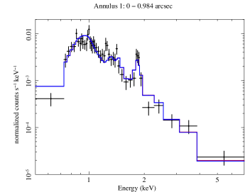
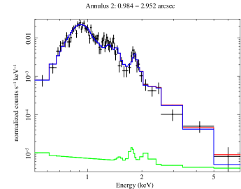
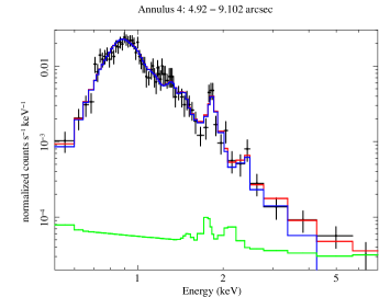
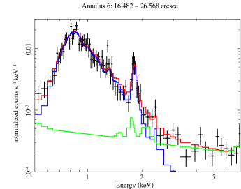
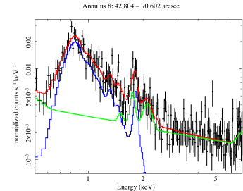
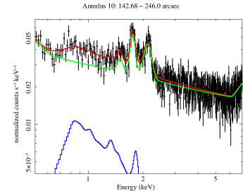
Figure 4.— Representative combined Chandra Cycle 19 spectra in the 0.5-7.0 keV band without any background subtraction. Also plotted are the best-fitting models (red) broken down into the separate contributions from the following: (1) hot gas and unresolved LMXBs from Mrk 1216 along with the CXB (blue), and (2) particle background (green). For the inner annuli, the broad peak near 1 keV is dominated by a great number of unresolved Fe L shell emission lines. The prominent feature near 1.8 keV is dominated by emission from He-like Si K$\alpha$. The modest bump near 1.4 keV is mostly H-like Mg K$\alpha$ with some contribution from other lines, most notably Fe L, blended in. At large radii, background lines of Si and S near 2 keV become increasingly apparent. Note all of the displayed spectra except that of Annulus 10 derive entirely from the ACIS-S3 (BI) CCD, while the majority of the emission in Annulus 10 derives from several FI CCDs (see §2).

4.2.1 Analysis of Projected Spectra

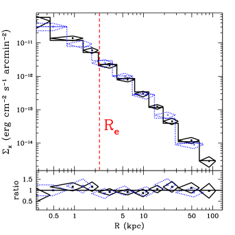
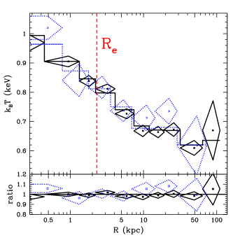
Figure 5.— The Cycle 19 Chandra data (solid black circles), $1\sigma$ errors (solid diamonds), and the best-fitting fiducial hydrostatic model (solid binned line) in each circular annulus on the sky for Mrk 1216. The corresponding quantities for the Cycle 16 data are plotted in dotted blue. (Left Panel) Surface brightness (0.5-7.0 keV). See the notes to Table 6 regarding the error bars on ${\Sigma_{\rm x}}$. (Right Panel) Projected emission-weighted temperature ($k_{B}T$). Also shown is the location of the stellar half-light radius ($R_{e}$). The bottom panels plot the data/model ratios. Note the displayed best-fitting model corresponds to the “Max Like” parameters (see §6.1) and is also indistinguishable from the best frequentist fit.

Table 6Hot Gas Properties

		$R_{\rm in}$	$R_{\rm out}$	$\Sigma_{\rm x}$ (0.5-7.0 keV)	$k_{B}T$	$Z_{\rm Fe}$	$Z_{\rm Mg}/Z_{\rm Fe}$	$Z_{\rm Si}/Z_{\rm Fe}$
Observation	Annulus	(kpc)	(kpc)	(ergs cm2 s-1 arcmin-2)	(keV)	(solar)	(solar)	(solar)
Chandra Cycle 19
	1	0.00	0.44	$\rm 4.50e-11\pm 1.76e-11$	$0.969\pm 0.027$	$1.04\pm 0.14$	$1.66\pm 0.43$	$1.64\pm 0.32$
	2	0.44	1.33	$\rm 1.38e-11\pm 2.24e-12$	$0.905\pm 0.018$	$1.00\pm 0.11$	$1.21\pm 0.16$	$0.79\pm 0.08$
	3	1.33	2.21	$\rm 5.99e-12\pm 1.11e-12$	$0.838\pm 0.019$	$1.00\pm 0.14$	tied	tied
	4	2.21	4.10	$\rm 2.08e-12\pm 3.36e-13$	$0.812\pm 0.016$	$0.91\pm 0.08$	$0.81\pm 0.11$	tied
	5	4.10	7.42	$\rm 7.90e-13\pm 1.12e-13$	$0.727\pm 0.017$	$0.74\pm 0.07$	tied	tied
	6	7.42	11.96	$\rm 2.98e-13\pm 5.85e-14$	$0.668\pm 0.020$	$0.75\pm 0.12$	$0.51\pm 0.10$	$1.30\pm 0.13$
	7	11.96	19.26	$\rm 1.23e-13\pm 1.97e-14$	$0.664\pm 0.019$	$0.68\pm 0.08$	tied	tied
	8	19.26	31.77	$\rm 4.51e-14\pm 9.55e-15$	$0.672\pm 0.023$	$0.71\pm 0.10$	$0.70\pm 0.14$	tied
	9	31.77	64.20	$\rm 1.21e-14\pm 2.58e-15$	$0.610\pm 0.025$	tied	tied	tied
	10	64.20	110.70	$\rm 2.89e-15\pm 9.96e-16$	$0.670\pm 0.101$	$0.36$	tied	tied
Chandra Cycle 16
	1	0.00	0.78	$\rm 3.07e-11\pm 7.62e-12$	$1.020\pm 0.040$	$0.98\pm 0.16$	$0.48\pm 0.17$	$0.63\pm 0.20$
	2	0.78	1.77	$\rm 9.33e-12\pm 2.51e-12$	$0.841\pm 0.056$	tied	tied	tied
	3	1.77	3.54	$\rm 2.50e-12\pm 6.80e-13$	$0.817\pm 0.038$	tied	tied	tied
	4	3.54	6.86	$\rm 1.00e-12\pm 2.19e-13$	$0.737\pm 0.038$	$0.78\pm 0.12$	tied	tied
	5	6.86	14.39	$\rm 2.69e-13\pm 6.39e-14$	$0.713\pm 0.044$	tied	tied	tied
	6	14.39	28.78	$\rm 6.93e-14\pm 1.57e-14$	$0.735\pm 0.044$	$0.63\pm 0.12$	tied	tied
	7	28.78	73.06	$\rm 8.90e-15\pm 2.08e-15$	$0.618\pm 0.101$	tied	tied	tied

The spectral model described above describes well the Cycle 19 data with a minimum C-statistic value of 2023.5 (in 2002 pha bins) with 1932 degrees of freedom (dof). The success of the model is on display in Figure 4 where we plot the spectra and best-fitting models for 5 representative annuli. The most noticeable spectral features are the broad bump near 1 keV dominated by a forest of emission lines from the Fe L shell and the strong Si K$\alpha$ line near 1.85 keV. Less noticeable, though still prominent in the inner annuli, is the Mg K$\alpha$ line complex near 1.4 keV. (Note for the Cycle 16 data we achieve a fit consistent with that obtained in Paper 1.)

The innermost and outermost annuli deserve special mention. Annulus 1 displays the most significant residuals from the best-fitting model resulting in a fit there that is of formally marginal quality. In Appendix C we study the central spectrum in detail and examine several possibilities to improve the fit, though at present we cannot confidently recommend a specific modification to the fiducial model. Since the background dominates in the outermost annulus (Annulus 10), the properties of the gas component there cannot be robustly determined. We found it necessary in the spectral fitting to restrict more strongly the gas parameter ranges there: i.e., ${k_{\rm B}T}=0.4-0.9$ keV. Guided by the average radial profiles of $Z_{\rm Fe}$ for groups and clusters obtained by Mernier et al. (2017), by default we fixed $Z_{\rm Fe}=0.36$ $Z_{\odot}$ in Annulus 10. Mernier et al. (2017) quote a scatter of $\sim\pm 0.09$ for ${Z_{\rm Fe}}$ over the radial range corresponding to Annulus 10, and we therefore use the range $Z_{\rm Fe}=0.27-0.45$ $Z_{\odot}$ as a systematic error in our HE models (§8.3).

We list the gas parameters measured for each annulus in Table 6 for the data sets. (We express the emission measure of the gas as a surface brightness unit – see the notes to the table.) In Figure 5 we plot the radial profiles of the surface brightness (${\Sigma_{\rm x}}$) and temperature (${k_{\rm B}T}$). As expected, ${\Sigma_{\rm x}}$ and ${k_{\rm B}T}$ are consistent in their overlap region (as is ${Z_{\rm Fe}}$). The lack of a big temperature jump in Annulus 1 of the Cycle 19 observation has implications for the mass of the SMBH (§7.3). The Cycle 19 data confirm and strengthen the similarity of the temperature profile of Mrk 1216 to that of the fossil group NGC 6482 (B17).

The profile of ${Z_{\rm Fe}}$ decreases with radius but is nearly constant over large stretches; i.e., ${Z_{\rm Fe}}\approx 1\,{Z_{\odot}}$ for $R\lesssim 2$ kpc and ${Z_{\rm Fe}}\approx 0.7\,{Z_{\odot}}$ for $R\approx 4-60$ kpc. This negative gradient in ${Z_{\rm Fe}}$ is very similar to those seen in several X-ray bright, massive elliptical galaxies and small groups like NGC 6482 (B17), NGC 5044 (Buote et al. 2003b) and others (e.g., Buote 2000a; Humphrey & Buote 2006; Rasmussen & Ponman 2009; Mernier et al. 2017).

Although the Mg and Si abundances are not as well constrained as Fe, we find the Cycle 19 observation does place interesting constraints on the radial variation of both ${Z_{\rm Mg}/Z_{\rm Fe}}$ and ${Z_{\rm Si}/Z_{\rm Fe}}$. The ${Z_{\rm Mg}/Z_{\rm Fe}}$ ratio appears to peak in the central $R\approx 2$ kpc with a value at least solar and is consistent with a constant ratio of $\approx 0.7$ solar at larger radius. The ${Z_{\rm Si}/Z_{\rm Fe}}$ profile is broadly similar to ${Z_{\rm Mg}/Z_{\rm Fe}}$ out to $R\approx 10$ kpc after which it increases significantly to ${Z_{\rm Si}/Z_{\rm Fe}}\approx 1.3$ solar. Since at large radius the Si abundance measurement becomes especially more challenging due to the increasing background level (both the continuum and the presence of an instrumental line), we regard our measurement there as provisional. Nevertheless, the ${Z_{\rm Mg}/Z_{\rm Fe}}$ and ${Z_{\rm Si}/Z_{\rm Fe}}$ profiles are broadly similar to mean profiles obtained from XMM-Newton for groups by Mernier et al. (2017).

For comparison, if we do not allow for a radial variation in either Mg or Si we obtain ${Z_{\rm Mg}/Z_{\rm Fe}}=0.83\pm 0.06$ solar and ${Z_{\rm Si}/Z_{\rm Fe}}=0.97\pm 0.07$ solar for the Cycle 19 data (which also gives ${Z_{\rm Fe}}\approx 0.80\,{Z_{\odot}}$ in Annulus 1). We use these results to perform a systematic error check on our fiducial models in §8. Notice also that these constant values of ${Z_{\rm Mg}/Z_{\rm Fe}}$ and ${Z_{\rm Si}/Z_{\rm Fe}}$ for the Cycle 19 data are consistent within the $\approx 1.5\sigma$ errors with the values obtained for the Cycle 16 data (Table 6), for which interesting constraints on the radial variation were not obtained.

Finally, the Cycle 19 results we have described in this section for the combined data are fully consistent with those obtained when performing a joint fit of the individual exposures (see Appendix A and Table 14).

4.2.2 Spectral Deprojection in Spherical Shells

If instead we perform spectral deprojection of the hot plasma in spherical shells with the projct model in xspec we find the C-statistic is reduced with respect to the fiducial case just described by only 0.6 with no obvious effect on the fractional residuals; e.g., the fit residuals for Annulus 1 look the same as obtained without deprojection (Figure 4 and 12).

We list the gas parameters for the deprojected case in Table 15 in Appendix B. The results for ${k_{\rm B}T}$ and the abundances are typically consistent within $\sim 1\sigma$ with those obtained without deprojection. As expected, the sizes of the error bars on all the parameters are larger, often twice as large, compared to those obtained with the fiducial projected model. We note the relatively large best-fitting value of ${k_{\rm B}T}=1.23$ keV obtained for Annulus 1 for the Cycle 16 data that is $\approx 2\sigma$ larger than the projected case, but also very consistent with the result obtained with projct by Werner et al. (2018).

The deprojected results just described made no account of any gas emission expected to exist exterior to Annulus 10 in the Cycle 19 data (or Annulus 7 of the Cycle 16 data). For comparison, we also examined adding a fixed gas contribution to the background annulus (§2) using the gas emission predicted by our best-fitting fiducial hydrostatic equilibrium model (Table 8). In this case the fit quality is unchanged, and the main differences are somewhat lower ${k_{\rm B}T}$ and density values in Annulus 10.

Since these deprojected models do not improve the fit, lead to larger parameter errors, and do not self-consistently address the emission expected outside the bounding annuli, throughout the paper we focus on the results obtained from the projected spectra.

4.2.3 Central Region: Quadrants

Table 7Hot Gas Properties in Quadrants

		$k_{\rm B}T$	norm	$\tilde{n}_{e}$	$\tilde{S}$	$\tilde{P}$
Annulus	Quadrant	(keV)	($10^{-5}$ cm-5)	(cm-3)	(keV cm2)	($10^{-10}$ erg cm-3)
2	1	$0.951\pm 0.038$	$1.07\pm 0.07$	$0.156\pm 0.005$	$3.29\pm 0.15$	$2.375\pm 0.120$
2	2	$0.842\pm 0.040$	$1.26\pm 0.07$	$0.169\pm 0.005$	$2.75\pm 0.14$	$2.279\pm 0.127$
2	3	$0.898\pm 0.045$	$1.08\pm 0.07$	$0.156\pm 0.005$	$3.10\pm 0.17$	$2.250\pm 0.132$
2	4	$0.892\pm 0.037$	$1.28\pm 0.07$	$0.171\pm 0.005$	$2.90\pm 0.13$	$2.440\pm 0.122$
2	Scatter	$0.043\pm 0.022$	$0.085\pm 0.030$	$0.043\pm 0.015$	$0.067\pm 0.024$	$0.032\pm 0.027$
3	1	$0.839\pm 0.033$	$1.04\pm 0.07$	$0.091\pm 0.003$	$4.13\pm 0.19$	$1.230\pm 0.063$
3	2	$0.828\pm 0.038$	$1.10\pm 0.07$	$0.094\pm 0.003$	$4.00\pm 0.20$	$1.249\pm 0.069$
3	3	$0.812\pm 0.039$	$0.97\pm 0.06$	$0.088\pm 0.003$	$4.10\pm 0.22$	$1.147\pm 0.067$
3	4	$0.913\pm 0.048$	$0.83\pm 0.06$	$0.081\pm 0.003$	$4.86\pm 0.28$	$1.191\pm 0.076$
3	Scatter	$0.045\pm 0.026$	$0.105\pm 0.032$	$0.054\pm 0.017$	$0.080\pm 0.030$	$0.033\pm 0.028$
4	1	$0.782\pm 0.032$	$1.58\pm 0.09$	$0.044\pm 0.001$	$6.27\pm 0.28$	$0.551\pm 0.027$
4	2	$0.827\pm 0.035$	$1.37\pm 0.08$	$0.041\pm 0.001$	$6.96\pm 0.32$	$0.543\pm 0.028$
4	3	$0.807\pm 0.036$	$1.19\pm 0.08$	$0.038\pm 0.001$	$7.10\pm 0.35$	$0.494\pm 0.027$
4	4	$0.808\pm 0.036$	$1.24\pm 0.08$	$0.039\pm 0.001$	$7.01\pm 0.34$	$0.506\pm 0.028$
4	Scatter	$0.020\pm 0.020$	$0.110\pm 0.032$	$0.054\pm 0.015$	$0.048\pm 0.022$	$0.046\pm 0.026$

Since the main objective of our paper is to infer the gravitating mass distribution using a hydrostatic equilibrium analysis, ideally we would want kinematic information for the hot plasma to inform and correct our analysis, especially for the central region where AGN feedback is expected to periodically inject energy into the hot gas. High spectral resolution observations of the Perseus cluster with Hitomi (Hitomi Collaboration et al. 2016) and in massive elliptical galaxies / small groups with the XMM-Newton RGS (e.g., Ogorzalek et al. 2017) indicate low amounts of turbulent pressure at the centers of these systems.

Another manifestation of non-hydrostatic behavior is via spatial fluctuations in the gas properties, in particular through the azimuthal scatter of properties within subregions of circular annuli (e.g., Vazza et al. 2011). The high spatial resolution combined with the moderate energy resolution of Chandra ACIS is well-suited for studying such azimuthal fluctuations in the central, high S/N regions of Mrk 1216. We were able to obtain useful constraints on the gas properties when dividing up Annuli 2, 3, and 4 into four quadrants, where for each annulus we fixed the metal abundances and background levels to the best-fitting results obtained for the whole annulus in §4.2.1.

Since hydrostatic equilibrium is a balance between pressure and gravity at any point, we use the inferred projected gas properties to construct three-dimensional proxies for the gas density, entropy, and pressure as follows. The normalization of the vapec model in xspec,

$${\rm\sc norm}\equiv 10^{-14}\int n_{e}n_{\rm H}{\rm dV}/\left(4\pi\left[\rm{D_{A}}\left(1+z\right)^{2}\right]\right),$$ (1)

is proportional to the emission measure, $\int n_{e}n_{\rm H}{\rm dV}$. We define a pseudo-electron number density ($\tilde{n}_{e}$) by dividing this emission measure by $V_{ij}^{\rm int}=(r_{j}^{2}-r_{i}^{2})^{3/2}$, taking the square root, and converting $n_{\rm H}$ to $n_{e}$. Here $r_{i}$ and $r_{j}$ are the inner and outer radii of the annulus on the sky representing the volume of the spherical shell intersected by the cylindrical annulus along the line-of-sight of the same radii (e.g., Kriss et al. 1983). We then use this pseudo-electron number density and the projected ${k_{\rm B}T}$ to define corresponding a pseudo-entropy and pseudo-pressure.

In Table 7 we list the results for these gas properties obtained for each quadrant for Annuli 2-4; see the caption to the table for the definitions of the quadrants. (We obtain consistent results for the scatter if we rotate the quadrants by 45 degrees.) To quantify the scatter between the quadrants of each sector, we follow Vazza et al. (2011) and define the quantity,

$${\rm Scatter}\equiv\sqrt{\frac{1}{N}\sum_{i=1}^{N}\left(\frac{y_{i}-\bar{y}}{\bar{y}}\right)^{2}},$$ (2)

where $y_{i}$ is the quantity in quadrant $i$, $\bar{y}$ is the average value of the quantity over the whole annulus, and $N=4$. The errors quoted for the scatter assume normal error propagation.

The largest scatter ($\approx 0.10$) occurs for norm while the other parameters have smaller scatters ($\lesssim 0.05$) in most cases. The hydrostatic equilibrium equation may be expressed in terms of the entropy and pressure having a dependence $S^{3/5}$ and $P^{2/5}$ respectively (e.g., Humphrey et al. 2008). The scatter in the pseudo-entropy and pseudo-pressure listed in Table 7 suggest $\lesssim 5\%$ azimuthal fluctuations in the hydrostatic equilibrium equation in the central region of Mrk 1216. Errors of this magnitude are less than the statistical errors on the inferred mass properties (e.g., Table 10).

4.2.4 Central Region: Image Residuals

The regions defined according to the residual image discussed in §3.3 have too few counts to clearly distinguish any differences in their spectra from the average spectrum of the annulus (or annuli) where they are located. The most significant differences we found occur for Region 4 defined in Table 5. This region has only 147 counts over 0.5-2.0 keV and straddles roughly equally the boundary between Annuli 2 and 3.

Since the background level is low in this small region ($1.3\arcsec$ radius), we found it convenient to use the blank-sky spectrum (§2) to account for both the CXB and particle background. If we fix the metal abundances to the average values of Annuli 2-3, we obtain a good fit with ${k_{\rm B}T}=0.79\pm 0.05$ keV, consistent the average values within $\approx 1.5\sigma$. The C-statistic is 24.4 for 31 pha bins and 28 dof.

If ${Z_{\rm Fe}}$ is allowed to vary, the C-statistic falls by $\approx 5$ and ${Z_{\rm Fe}}$ fits to a much lower value, ${Z_{\rm Fe}}=0.60\pm 0.15\,{Z_{\odot}}$, a little less than $3\sigma$ below the average value of $\approx 1\,{Z_{\odot}}$. We strongly suspect that this reflects the Fe Bias (e.g., Buote 2000b), since we obtain nearly the same reduction in the C-statistic if instead we add a second temperature component with the same abundances all fixed at 1 solar. The resulting 2T fit gives best-fitting ${k_{\rm B}T}$ values of 0.6 keV and 1.1 keV for the temperature components with approximately the same emission measure for each. However, if we allow ${Z_{\rm Fe}}$ to vary in the 2T model, it still fits to $\approx 0.60\,{Z_{\odot}}$. These solutions provide potentially interesting evidence for inhomogeneous gas cooling and metal enrichment, though we believe the fact this region is a deficit does not favor a cooling scenario. Higher quality data are needed to clarify the gas properties and their implications.

5. Hydrostatic Equilibrium Models

Table 8Fiducial Bayesian Hydrostatic Equilibrium Model

			Prior
Component	Model	Parameter	Type	Range	Units	Best Fit	Max Like	Std. Dev.
Boundary Condition	$P_{\rm gas}(r=10\,\rm kpc)$	$P_{\rm ref}$	Flat Log	$10^{-12}-10^{-9}$	$10^{-11}$ erg cm-3	1.67	1.69	0.06
Entropy	Broken Power Law	$s_{0}$	Flat	$0-10$	keV cm2	1.62	1.25	0.32
	& constant	$s_{1}$	Flat Log	$0.001-1$	keV cm2	0.16	0.20	0.15
		$\alpha_{1}$	Flat	$1-5$		3.09	3.38	0.91
		$r_{\rm b,1}$	Flat	$0.25-1$	kpc	0.66	0.46	0.12
		$\alpha_{2}$	Flat	$0.1-3$		0.78	0.77	0.05
		$r_{\rm b,2}$	Flat	$5-18.5$	kpc	16	18	2
		$\alpha_{3}$	Flat	$1-5$		2.25	3.54	0.74
		$r_{\rm b,3}$	Flat	$19-25$	kpc	22	20	2
		$\alpha_{4}$	Flat Log	$0.05-5$		0.61	0.67	0.19
		$r_{\rm b,4}$	Flat	$26-80$	kpc	58	50	14
		$\alpha_{5}$	Flat	$0.5-2$		1.08	0.99	0.31
Black Hole	Point Mass	$M_{\rm BH}$	Lognorm	$M_{\rm BH}-\sigma$	$10^{9}\,M_{\odot}$	0.8	0.6	0.4
Stellar Mass	MGE $H$-band	$M_{\rm stars}/L_{\rm H}$	Flat	$0.2-5$	$M_{\odot}/L_{\rm H,\odot}$	1.19	1.22	0.11
	(sphericalized)
Dark Matter	NFW	norm	Flat Log	0.5-100	$10^{12}\,M_{\odot}$	1.9	1.9	0.4
		$r_{s}$	Flat	$2-60$	kpc	12.1	12.0	2.2

We use a spherical, entropy-based solution of the hydrostatic equilibrium (HE) equation to infer the mass distribution from the radial gas properties measured from the Chandra observations (Humphrey et al. 2008; for a review of the relative virtues of this and other HE methods see Buote & Humphrey 2012a); we discuss the spherical approximation in §8.5. Our implementation of the entropy-based method follows closely that described by B17, and we refer the reader to that paper for details. Below we summarize the principal models used for Mrk 1216.

• Entropy: We represent the entropy proxy ($S\equiv k_{\rm B}Tn_{e}^{-2/3}$) in units of keV cm² by, $S(r)=s_{0}+s_{1}f(r_{0.25})$, where $s_{0}$ is a constant, $f(r_{0.25})$ is a dimensionless power-law with possibly one or more break radii, $r_{0.25}$ is the radius in units of 0.25 kpc, and $s_{1}=S(0.25\,{\rm kpc})-s_{0}$; see equation (3) of B17. Our fiducial model employs four break radii. In addition, we demand that at large radius the radial logarithmic entropy slope match the value $\approx 1.1$ from cosmological simulations with only gravity (e.g., Tozzi & Norman 2001; Voit et al. 2005). We adopt a fiducial radius of $r_{\rm b,baseline}=150$ kpc above which the 1.1 slope applies.

• Pressure: We express the free parameter associated with the boundary condition for the HE equation as a pressure located at a radius 10 kpc which we denote as the “reference pressure” $P_{\rm ref}$.

• Stellar Mass: We employ a spherically averaged version of the ellipsoidal multi-gauss expansion (MGE) model of the HST $H$-band light reported by Y17. We convert the stellar light profile to stellar mass with the stellar mass-to-light ratio ($M_{\rm stars}/L_{\rm H}$) parameter that is free to vary.

• Dark Matter: Our fiducial model represents the dark matter halo by an NFW profile (Navarro et al. 1997) with free parameters a scale radius ($r_{s}$) and normalization that we convert to a halo concentration and mass computed for a radius of a specific overdensity. For comparison we also consider the Einasto (Einasto 1965) and CORELOG (e.g., Buote & Humphrey 2012c) models. Finally, we also explore models that modify these DM profiles by “adiabatic contraction” (AC). Here we consider two variants of AC – classic “strong” AC as originally proposed by Blumenthal et al. (1986) and a “weak” AC model proposed by Dutton et al. (2015) which they call “Forced Quenched.” See B17 for details of our implementation of these AC models.

• SMBH: We include a central point mass to represent a SMBH with mass $M_{\rm BH}$. Unlike Paper 1 where we fixed $M_{\rm BH}=4.9\times 10^{9}\,M_{\odot}$ to the stellar dynamical value obtained by Walsh et al. (2017) in our fiducial model, here we allow it to be a free parameter subject to different priors (see below in §6).

We list the free parameters for the fiducial HE model in Table 8. The 16 free parameters of the model are constrained by 17 measurements each of ${k_{\rm B}T}$ and ${\Sigma_{\rm x}}$; i.e., 34 total data points – 14 and 20 respectively from the Cycle 16 and 19 observations.

6. Model Fitting Methodology

6.1. Bayesian Method

The primary method we adopt to fit the HE models to the Chandra data employs a Bayesian nested sampling procedure based on the MultiNest code v2.18 (Feroz et al. 2009) (see B17 for details). In Table 8 we list the priors adopted for each free parameter. We use flat priors in most cases and flat priors on the decimal logarithm for a few parameters with ranges spanning multiple orders of magnitude. For the black hole mass our fiducial prior is based on the $M_{\rm BH}-\sigma$ relation of van den Bosch (2016); i.e., a median value ${M_{\rm BH}}=2.1\times 10^{9}\,{M_{\odot}}$ using the stellar velocity dispersion for Mrk 1216 listed in Table 1. Since van den Bosch (2016) quote an intrinsic scatter of 0.49 in $\log_{10}{M_{\rm BH}}$, we adopt a lognormal prior with mean $\log_{10}{M_{\rm BH}}=9.32$ and standard deviation equal to the intrinsic scatter.

For the Bayesian analysis we quote two “best” values for each free parameter: (1) the mean parameter value of the posterior which we call the “Best Fit”, and (2) the parameter value that maximizes the likelihood, which we call “Max Like.” Unless otherwise stated, all errors quoted for the parameters are the standard deviation ($1\sigma$) of the posterior.

6.2. Frequentist Method

We also perform frequentist $\chi^{2}$ fits of the HE models for comparison to the results obtained with the Bayesian fits. Despite its shortcomings (e.g., Andrae et al. 2010), we also prefer the frequentist $\chi^{2}$ approach for model selection which, unlike Bayes factors, does not depend on the priors. For the frequentist fits we use the minuit fitting package that is part of the root v6.10 software suite.

7. Results

Table 9Quality of Frequentist $\chi^{2}$ Fits

Model	$\chi^{2}$	dof
Fiducial	11.9	18
Joint Fit of Cycle 19 Obs.	13.7	18
No Stars	40.5	19
No DM Halo	395.8	20
Cycle 19 Only	4.5	4
0 Brk Entropy	28.3	26
1 Brk Entropy	17.5	24
Sersic Stars 2MASS	11.0	18
Einasto DM	11.1	18
Corelog DM	10.9	18
Strong AC	14.8	18
Weak AC	11.2	18
Weak AC Einasto	10.7	18
Fixed Over-Massive BH	14.2	19
Fixed $M-\sigma$ BH	12.6	19

Table 10Stellar and Total Mass

	$M_{\star}/L_{H}$	$M_{\rm BH}$	$c_{2500}$	$M_{2500}$	$c_{500}$	$M_{500}$	$c_{200}$	$M_{200}$
	($M_{\odot}L_{\odot}^{-1}$)	$(10^{9}\,M_{\odot})$		$(10^{12}\,M_{\odot})$		$(10^{12}\,M_{\odot})$		$(10^{12}\,M_{\odot})$
Best Fit	$1.19\pm 0.11$	$0.8\pm 0.4$	$11.1\pm 1.6$	$3.2\pm 0.3$	$21.1\pm 3.0$	$4.5\pm 0.5$	$30.4\pm 4.3$	$5.3\pm 0.6$
(Max Like)	$(1.22)$	$(0.6)$	$(10.9)$	$(3.2)$	$(20.7)$	$(4.4)$	$(29.9)$	$(5.3)$
1 Brk Entropy	$-0.04$	$-0.1$	$0.8$	$-0.1$	$1.5$	$-0.2$	$2.1$	$-0.2$
BH Flat Prior	$-0.03$	$0.2$	$0.4$	$-0.1$	$0.7$	$-0.1$	$1.0$	$-0.1$
BH Flat Logspace Prior	$0.03$	$-0.5$	$-0.1$	$0.0$	$-0.3$	$0.0$	$-0.4$	$0.0$
Fixed Over-Massive BH	$-0.46$	$4.1$	$3.7$	$-0.4$	$6.8$	$-0.6$	$9.8$	$-0.8$
Fixed ${M_{\rm BH}-\sigma}$ BH	$-0.13$	$1.3$	$1.0$	$-0.1$	$1.8$	$-0.2$	$2.6$	$-0.3$
Sersic Stars 2MASS	$0.04$	$-0.0$	$-1.5$	$0.3$	$-2.8$	$0.5$	$-4.0$	$0.6$
Einasto	$-0.07$	$0.0$	$-1.0$	$0.4$	$-2.1$	$0.5$	$-3.2$	$0.5$
Strong AC	$-0.40$	$-0.0$	$-3.3$	$0.6$	$-6.1$	$1.1$	$-8.8$	$1.4$
Weak AC	$-0.06$	$-0.0$	$-2.5$	$0.3$	$-4.6$	$0.6$	$-6.5$	$0.8$
Weak AC Einasto	$-0.13$	$0.0$	$-3.6$	$0.9$	$-6.6$	$1.6$	$-9.6$	$1.9$
Joint Fit of Cycle 19 Obs.	$-0.04$	$-0.0$	$1.6$	$-0.2$	$2.9$	$-0.4$	$4.2$	$-0.5$
Constant $Z_{\alpha}/{Z_{\rm Fe}}$	$0.13$	$-0.0$	$-0.6$	$0.1$	$-1.1$	$0.2$	$-1.6$	$0.2$
Annulus 10 $\Delta{Z_{\rm Fe}}$	${}^{+0.02}_{-0.00}$	$-0.0$	${}^{+0.4}_{-0.4}$	${}^{+0.2}_{-0.1}$	${}^{+0.7}_{-0.7}$	${}^{+0.2}_{-0.2}$	${}^{+1.0}_{-1.1}$	${}^{+0.3}_{-0.2}$
Deproj	$-0.16$	$0.0$	$1.3$	$-0.2$	$2.5$	$-0.3$	$3.9$	$-0.2$
Distance	$-0.16$	$0.0$	$-1.1$	$0.2$	$-2.1$	$0.4$	$-2.9$	$0.6$

The best-fitting Bayesian fiducial model is displayed along with the ${k_{\rm B}T}$ and ${\Sigma_{\rm x}}$ data points in Figure 5. The corresponding best-fitting parameter values and $1\sigma$ errors are listed in Table 8. The fit is excellent for both the Cycle 16 and Cycle 19 observations. The frequentist fit (not shown) yields a nearly identical result with $\chi^{2}=11.9$ for 18 dof (Table 9). The formal probability of obtaining a smaller value of $\chi^{2}$ is $\approx 15\%$, indicating the fit is marginally “too good” to happen by chance. However, we do not believe the error bars have been overestimated. When fitting the Cycle 19 data alone we obtain $\chi^{2}=4.49$ for 4 (dof, see Table 9) with a very reasonable probability of $66\%$ for obtaining a smaller $\chi^{2}$ value (and a corresponding significance of only $34\%$ to reject the model). The Cycle 16 data also give a very reasonable $\chi^{2}$ value when fitted on their own – see Paper 1.

In Figure 6 we show the total mass profile of the Bayesian fiducial model broken down into its constituents. Within the central $0.44$ kpc corresponding to the radius of Annulus 1 of the Cycle 19 observation, the DM and SMBH contribute nearly equally to the total mass, while the stellar mass dominates both. The DM and stars contribute equally at $r\approx 3.9$ kpc ($\sim 1.7R_{e}$) after which the DM dominates all components. The gas mass does not equal the stellar mass until $r\sim 170$ kpc.

We will refer to the best-fitting “virial radii” of the fiducial model evaluated at a few reference overdensities (see §5.3 of B17 for details on their computation): ${r_{2500}}=130\pm 5$ kpc, ${r_{500}}=248\pm 10$ kpc, and ${r_{200}}=358\pm 14$ kpc. The Cycle 19 gas measurements extend to $\approx 0.85{r_{2500}}$. Since, however, the outer bin width is rather large, more relevant for discussing the properties of the HE models is the average bin radius (eqn. 10 of McLaughlin 1999) $\approx 90$ kpc or $\approx 0.7{r_{2500}}$.

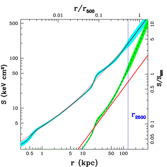
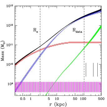
Figure 6.— Results for the Bayesian HE modeling of Mrk 1216. The curved lines and associated shaded regions in both plots show the mean (i.e., “best fit”) and standard deviation of the posterior as a function of radius for the quantity of interest; i.e., entropy or mass. (Left Panel) Radial profile of the entropy (black) and $1\sigma$ error region (cyan) for the fiducial hydrostatic model. For comparison with a dotted red line we show the best-fitting entropy profile with only one break radius which follows the fiducial 4-break model very closely. The upper horizontal axes gives the radius in units of ${r_{500}}$ while the vertical axis on the right shows the entropy rescaled by $S_{500}=48.0$ keV cm² (see eqn. 3 of Pratt et al. 2010). The baseline $r^{1.1}$ profile obtained by cosmological simulations (Voit et al. 2005) with only gravity is shown as a red line. The result of rescaling the entropy profile by $\propto f_{\rm gas}^{2/3}$ (Pratt et al. 2010) is shown by the black dashed line (and green $1\sigma$ region). (Right Panel) Radial profiles of the total mass (black) and individual mass components of the fiducial hydrostatic model: total NFW DM (blue), stars (red), hot gas (green), and SMBH (magenta). The black vertical lines in the bottom right corner indicate the best-fit virial radii; i.e., from left to right: $r_{2500}$, $r_{500}$, and $r_{200}$. The vertical dashed lines indicate the location of the stellar half-light radius $(R_{e})$ and the outer extent of the Chandra data analyzed $(R_{\rm data})$.

7.1. Entropy

In Paper 1 we found the Cycle 16 data were described well by an entropy profile consisting of only a constant and a power-law with no breaks in radius. Fitting such a model jointly to the Cycle 16 and Cycle 19 still results in a formally acceptable fit: $\chi^{2}=28.3$ for 26 dof (“0 Brk Entropy” in Table 9). However, when adding a break radius, the fit improves significantly ($\chi^{2}=17.5$ for 24 dof, “1 Brk Entropy” in Table 9). The 1-break entropy profile has a poorly constrained break radius $r_{\rm b,1}=7\pm 5$ kpc, and its best-constrained parameter is the power-law exponent exterior to the break radius ($\alpha_{2}=0.93\pm 0.05$). Adding more breaks reduces $\chi^{2}$ but does not lead to a statistically significant improvement in the fit.

Nevertheless, we add more break radii to provide greater flexibility in the entropy model for the following reason. When comparing models with different assumptions in the mass components (e.g., fixed over-massive SMBH, Einasto DM halo, AC, etc.) we want potential differences in the fits to be determined by differences in the form of the mass components not the precise form of the assumed entropy profile. HE and convective stability only requires that the entropy profile increase monotonically with radius. Consequently, we added break radii until the value of $\chi^{2}$ changed by less than 1.

We followed this procedure and arrived at an entropy profile with four breaks having break radii $\approx 0.7$, 16, 22, and 58 kpc. (We obtained this final result after initially using larger prior ranges than indicated in Table 8.) The inner break adds flexibility when testing different SMBH priors while the others allow for flexibility primarily for the DM halo models. The two break radii in the middle are rather close together indicating a fairly abrupt jump in entropy near 20 kpc. The slope parameter at large radius is not well-constrained and is consistent with the $r^{1.1}$ profile from gravity-only simulations (Voit et al. 2005). Although this 4-break entropy profile is the fiducial model we employ (§5, Table 8), in §8 we compare to results obtained with the 1-break entropy profile as a systematics error check. (The best-fitting 1-break model is plotted in Figure 6 as a red dotted line.)

In Figure 6 we plot the entropy profile of the Bayesian fiducial model along with the $\sim r^{1.1}$ theoretical entropy profile produced by gravity-only cosmological simulations (Voit et al. 2005). The entropy profile of Mrk 1216 is remarkably similar to those we have obtained previously for other massive, fossil-like elliptical galaxies, NGC 720 (Humphrey et al. 2011), NGC 1521 (Humphrey et al. 2012), and NGC 6482 (B17). That is, within a radius $\sim{r_{2500}}$, the entropy profile greatly exceeds the theoretical gravity-only profile. In addition, when the observed entropy profile is rescaled by $\sim f_{\rm gas}^{2/3}$ (Pratt et al. 2010), the result broadly matches the gravity-only profile. The success of this rescaling indicates that for $r\lesssim{r_{2500}}$ the feedback energy responsible for raising the entropy in that region is consistent with having spatially rearranged the gas rather than raising its temperature, as also is observed for galaxy clusters (Pratt et al. 2010).

We see, however, that as the entropy approaches ${r_{2500}}$ this rescaling becomes increasingly less successful. Very similar behavior is observed for NGC 1521 (Humphrey et al. 2012), and NGC 6482 (B17). Perhaps for Mrk 1216 and these galaxies at larger radius the feedback energy heated the gas by raising its temperature indicating a different feedback mechanism prevails for $r\gtrsim{r_{2500}}$. It is also noteworthy that interior to $\approx 0.6{r_{2500}}$ (77 kpc) the cooling time is less than the age of the Universe (see Figure 9), and thus the details of gas cooling may be responsible for the apparent transition in the rescaling behavior as the radius approaches ${r_{2500}}$.

7.2. Pressure

The pressure profile of the fiducial Bayesian HE model (not shown) is extremely similar to that of NGC 6482 (see §6.3 and Figure 5 of B17). Between radii $\approx 0.1-0.7\,{r_{500}}$ the pressure profile broadly matches the “universal” pressure profile determined for galaxy clusters by Arnaud et al. (2010), while at smaller and larger radii the observed profile is clearly a different shape. While the results for $r\gtrsim 0.7{r_{500}}$ are provisional owing to the limited data range, the different shape at smaller radius is robust implying a breakdown in the mass scaling of the universal pressure profile and, presumably, the greater importance of non-gravitational energy in shaping the thermodynamical properties of the gas in galaxy/group-scale halos.

7.3. SMBH

In Paper 1 we analyzed the Cycle 16 observation and obtained a Bayesian constraint on the black hole mass, $M_{\rm BH}=(5\pm 4)\times 10^{9}\,M_{\odot}$, for a flat prior very consistent with the stellar dynamical measurement, ${M_{\rm BH}}=(4.9\pm 1.7)\times 10^{9}\,M_{\odot}$, of Walsh et al. (2017). When instead using a flat prior on $\log_{10}{M_{\rm BH}}$ (“Flat Logspace Prior”), we obtained a smaller value, $M_{\rm BH}=(1.4\pm 1.7)\times 10^{9}\,M_{\odot}$, still consistent with the stellar dynamical measurement within the large errors. Our best-fitting model in Paper 1 for the flat prior on ${M_{\rm BH}}$ predicted a projected emission-weighted temperature, ${k_{\rm B}T}\sim 1.18$ keV, within the central $R=1\arcsec$; i.e,. the region corresponding to Annulus 1 of the new Cycle 19 observation.

As is readily apparent from the temperature profile displayed in Figure 5 and the ${k_{\rm B}T}$ values listed in Table 6 we measure a much smaller temperature in Annulus 1 with the Cycle 19 observation: ${k_{\rm B}T}=0.969\pm 0.027$ keV implying a smaller value of ${M_{\rm BH}}$ than indicated in Paper 1. (Note only for Annulus 1 was the predicted ${k_{\rm B}T}$ from Paper 1 inaccurate; e.g., for Annulus 2 the predicted value was $0.910$ keV compared to the value measured of ${k_{\rm B}T}=0.905\pm 0.018$ keV.) For a flat prior, our joint fit of the Cycle 16 and Cycle 19 data gives, ${M_{\rm BH}}=(1.0\pm 0.6)\times 10^{9}\,{M_{\odot}}$, with a 99.9% upper limit, ${M_{\rm BH}}\leq 3.9\times 10^{9}\,{M_{\odot}}$. The flat logspace prior fits to even lower values approaching the lower limit of the adopted prior range, ${M_{\rm BH}}=(0.3\pm 0.2)\times 10^{9}\,{M_{\odot}}$ with a 99.9% upper limit, ${M_{\rm BH}}\leq 1.1\times 10^{9}\,{M_{\odot}}$ .

As mentioned in the notes to Table 9, the frequentist fit also gives ${M_{\rm BH}}$ consistent with the adopted lower fit boundary. However, when fixing ${M_{\rm BH}}$ to the stellar dynamical value, $\chi^{2}$ only increases by 2.3 (“Fixed Over-Massive BH” in Table 9). According to the F-Test, the fiducial model is $\approx 92\%$ more probable; i.e., the preference for a small value of ${M_{\rm BH}}$ is less than a $2\sigma$ effect for the frequentist fit.

Fixing ${M_{\rm BH}}$ to the stellar dynamical value leads to a smaller inferred value for ${M_{\star}/L_{H}}$ (“Fixed Over-Massive BH” in Table 10). The Bayesian fit gives, ${M_{\star}/L_{H}}=0.73\pm 0.13$ solar with a 99.9% upper limit, ${M_{\star}/L_{H}}\leq 0.99$ solar, significantly less than ${M_{\star}/L_{H}}=1.2$ solar expected for a Kroupa IMF (§7.4). The frequentist fit gives ${M_{\star}/L_{H}}=0.96\pm 0.13$ solar which is $\sim 2\sigma$ discrepant.

Therefore, the Bayesian fits clearly disfavor the over-massive SMBH, as indicated by the values inferred for ${M_{\rm BH}}$ when it is fitted freely and for ${M_{\star}/L_{H}}$ when ${M_{\rm BH}}$ is fixed to the stellar dynamical value. (The significantly larger $c_{200}$ value provides more evidence against the over-massive SMBH model – see §7.6 and §9.1.) The frequentist analysis also disfavors the over-massive SMBH but at a much lower significance level ($\sim 2\sigma$).

Given the dependence of the constraints on the priors, by default we adopt a prior on ${M_{\rm BH}}$ consistent with the ${M_{\rm BH}-\sigma}$ relation of van den Bosch (2016) – see §6.1. In §9.3 we discuss the implications of the smaller values inferred for ${M_{\rm BH}}$ compared to the stellar dynamics measurement.

7.4. Stellar Mass and IMF

The Chandra data clearly require the stellar mass component. If the stellar mass is omitted, the frequentist fit gives $\chi^{2}=40.5$ for 19 dof (Table 9), which is an increase of 28.6 over the fiducial model with one extra dof. The strong need for the stellar component translates to a good constraint on stellar mass-to-light ratio; i.e., ${M_{\star}/L_{H}}=1.19\pm 0.11$ for the fiducial Bayesian model (Table 10). This value agrees very well with that expected from single-burst stellar population synthesis (SPS) models with a Kroupa IMF (${M_{\star}/L_{H}}=1.2$), but is significantly lower than predicted for a Salpeter IMF (${M_{\star}/L_{H}}=1.7$ solar); see Walsh et al. (2017) for more information about these SPS estimates.

Our fiducial measurement also agrees very well with the value $1.3\pm 0.3$ solar (statistical error) obtained by the stellar dynamical study of Walsh et al. (2017), with a factor of $\approx 2.5$ higher precision. Y17’s stellar dynamical measurement gives a value about $50\%$ larger, ${M_{\star}/L_{H}}=1.9^{+0.5}_{-0.4}$ solar, at $\approx 2\sigma$ significance, which agrees better with the SPS value for a Salpeter IMF. In §9.2 we discuss these stellar dynamical measurements and their sensitivity to the assumed DM halo concentration.

Most of the systematic errors we considered do not change ${M_{\star}/L_{H}}$ by more than the $1\sigma$ statistical error (Table 10). Of key importance is that if we use a different model to represent the stellar light profile (§8.6), we obtain ${M_{\star}/L_{H}}=1.23$ solar, very consistent with the MGE result. Much smaller values of ${M_{\star}/L_{H}}$ are given by a few models, “Fixed Over-Massive BH” (§7.3), “Strong AC” (§7.5), and to a lesser extent “Deproj” and “Distance”’, which we believe is notable evidence disfavoring these models. The “Constant $Z_{\alpha}/{Z_{\rm Fe}}$” test give the largest positive shift in ${M_{\star}/L_{H}}$.

The very good agreement we find with the value of ${M_{\star}/L_{H}}$ we measure and SPS models with a Kroupa IMF is also very consistent with what we find for other fossil-like massive elliptical galaxies from X-ray HE analysis. This evidence for a Kroupa IMF is in stark contrast to the support typically found for a Salpeter IMF from stellar dynamics and lensing studies of massive elliptical galaxies (see discussion in § 8.3 of B17).

7.5. Dark Matter: NFW and Alternatives

Of the SMBH, stars, and DM, by far the most important component needed to describe the X-ray emission is the DM (Table 9). If the DM halo is omitted from the fiducial model, the frequentist fit gives $\chi^{2}=395.8$ for 20 dof; i.e., the F-test gives a tiny probability ($2\times 10^{-14}$) that the “No DM Halo” model is preferred over the fiducial model with DM. While the DM component is clearly required, the Chandra data do not distinguish between the different DM models we investigated. The Einasto and CORELOG models give minimum $\chi^{2}$ values that are $<1$ from that obtained for the fiducial model and with the same number of dof (Table 9). The weak AC model applied to the NFW and Einasto models changes the fit quality very little. The strong AC NFW model has a $\chi^{2}$ value that is a little larger (i.e., by 2.9) but is still a good fit.

As noted above in §7.4, the strong AC model gives a much smaller ${M_{\star}/L_{H}}$, which we believe disfavors that model. The CORELOG model (not shown in Table 10) is peculiar in that the “Best Fit” and “Max Like” values for ${M_{\star}/L_{H}}$ differ significantly; i.e. ${M_{\star}/L_{H}}\sim 0.7$ solar for “Best Fit” and ${M_{\star}/L_{H}}\sim 1.2$ solar for “Max Like” with $1\sigma$ error $\pm 0.2$ solar, where the larger “Max Like” values are favored to match the SPS models (§7.4).

These results are very consistent with those obtained for NGC 6482 (B17).

7.6. Halo Concentration and Mass

In Paper 1 we obtained tentative evidence for an “over-concentrated” NFW DM halo compared to the general halo population. Our Bayesian fiducial model fitted to the Cycle 16 Chandra data yielded a Best Fit virial mass, $M_{200}=(9.6\pm 3.7)\times 10^{12}\,M_{\odot}$ and concentration, $c_{200}=17.5\pm 6.7$ considerably larger than the median $\Lambda$CDM value of $\approx 7$ (e.g., Dutton & Macciò 2014). Intriguingly, we found the Max Like best-fitting value suggested an even more extreme outlier from the $\Lambda$CDM relation: $c_{200}=25.9$ and $M_{200}=5.1\times 10^{12}\,M_{\odot}$.

Adding the much deeper Cycle 19 Chandra observations to our analysis confirms the higher concentration solution from Paper 1. In Table 10 we list the concentration and mass for overdensities $\Delta=200,$ 500, and 2500. Now the Best Fit and Max Like values agree extremely well. The values we measure, $c_{200}=30.4\pm 4.3$ and $M_{200}=(5.3\pm 0.6)\times 10^{12}\,M_{\odot}$, indicate an extreme outlier to the median $\Lambda$CDM relation (see §9.1).

The AC models give statistically significant lower values of $c_{200}$, with Strong AC giving a larger reduction $(\approx 9)$ than Weak AC $(\approx 7)$. As noted above in §7.4, the Strong AC model gives an uncomfortably low ${M_{\star}/L_{H}}$ whereas Weak AC gives ${M_{\star}/L_{H}}$ fully compatible with the fiducial model. The Fixed Over-Massive BH model gives the largest increase in $c_{200}(+9.8)$, which disfavors the model as an even more extreme outlier from the median $\Lambda$CDM relation (§9.1). Note, however, that the frequentist fit for this model increases $c_{200}$ by only $\approx 4$; i.e., the evidence is mostly directed against the Bayesian version of the Fixed Over-Massive BH model (also see above in §7.3).

The Einasto model and Weak AC Einasto models behave analogously to the NFW versions except with $c_{200}$ shifted lower by $\sim 3$. We reiterate that these various DM models cannot be distinguished in terms of their fit quality (§7.5).

All of the results described in this section, in particular the evidence that Mrk 1216 is an extreme outlier in the $\Lambda$CDM $c_{200}-M_{200}$ relation, are very consistent with the fossil galaxy/group NGC 6482 (B17). In §9.1 we discuss further implications of the high value measured for $c_{200}$.

7.7. Density Slope and DM Fraction

Table 11Mass-Weighted Total Density Slope and DM Fraction

Radius	Radius	Fiducial		Weak AC + Einasto
(kpc)	($R_{e}$)	$\langle\gamma\rangle$	$f_{\rm DM}$	$\langle\gamma\rangle$	$f_{\rm DM}$
1.1	0.5	$2.12\pm 0.04$	$0.18\pm 0.04$	$2.05\pm 0.04$	$0.27\pm 0.05$
2.3	1.0	$2.04\pm 0.05$	$0.34\pm 0.05$	$2.02\pm 0.04$	$0.43\pm 0.06$
4.6	2.0	$1.93\pm 0.03$	$0.54\pm 0.05$	$1.99\pm 0.02$	$0.60\pm 0.05$
9.2	4.0	$1.91\pm 0.02$	$0.71\pm 0.03$	$1.97\pm 0.02$	$0.74\pm 0.03$
11.5	5.0	$1.94\pm 0.03$	$0.76\pm 0.03$	$1.98\pm 0.02$	$0.78\pm 0.03$
23.0	10.0	$2.08\pm 0.05$	$0.85\pm 0.01$	$2.02\pm 0.04$	$0.87\pm 0.02$

In Table 11 we list the mass-weighted slope $(\langle\gamma\rangle)$ and DM fraction $(f_{\rm DM})$ for the Bayesian fiducial model evaluated at radii for several multiples of $R_{e}$. For $r=R_{e}$ we obtain $\langle\gamma\rangle=2.04\pm 0.05$ and $f_{\rm DM}=0.34\pm 0.05$ which differ significantly from the average values obtained by Y17 for their sample of 16 CEGs ($\langle\gamma\rangle=2.3$, $f_{\rm DM}=0.11$). We discuss the principal reason for the discrepancy between our results and those of Y17 in §9.2. We note that the AC models give even larger DM fractions for Mrk 1216; e.g., the Weak AC+Einasto model result shown in Table 11.

The mass-weighted slope we measure for Mrk 1216 within $r=R_{e}$ is less than the average slopes of local massive ETGs ($2.15\pm 0.03$, intrinsic scatter 0.10) determined by stellar dynamics (Cappellari et al. 2015). The local ETGs also have a smaller DM fraction (0.19, accounting for the higher mass range of the CEGs –see Y17). These differences between the local “normal” ETGs and Mrk 1216 presumably reflect the unusual and very high $c_{200}$ we measure for Mrk 1216; i.e., higher DM concentration means more DM near the center (higher $f_{\rm DM}$) which translates to a smaller slope due to the higher weighting of the NFW (or Einasto) profile with a flatter slope than the stellar profile.

Studies of ETGs that combine strong lensing with stellar dynamics have found a large range of DM fractions within $R_{e}$, including several with values consistent with (or larger than) what we have found for Mrk 1216 (e.g., Barnabè et al. 2011; Sonnenfeld et al. 2015). The large DM fractions in the lensing/SD studies probably do not reflect unusually high $c_{200}$ like Mrk 1216; i.e., those galaxies were not selected to be early forming objects like Mrk 1216 (or NGC 6482), and thus they should not often possess $c_{200}$ values that deviate extremely from the $\Lambda$CDM $c_{200}-M_{200}$ relation.

Recently, Wang et al. (2018) have used the IllustrisTNG simulation to show that massive ETGs in $\Lambda$CDM have $\langle\gamma\rangle=2.003$ with a scatter of $0.175$ over the radial range $0.4-4\,R_{e}$ with the slope changing little for redshifts below 2. The slope we measure for Mrk 1216 is consistent with these results (Table 11). Using the same simulation Lovell et al. (2018, see their Figure 12) obtain $f_{\rm DM}$ within $5R_{e}$ consistent with our measurements but within $1R_{e}$ they find large values ($f_{\rm DM}\sim 0.6$). Using a different simulation Remus et al. (2017) find a large range of DM fractions within $1R_{e}$ consistent with what we find for Mrk 1216. Interestingly, both Remus et al. (2017) and Lovell et al. (2018) obtain smaller DM fractions within $1R_{e}$ at $z=2$; e.g., $f_{\rm DM}\approx 10\%$ (Remus et al. 2017). If Mrk 1216 is truly a nearby analog of a $z\approx 2$ galaxy, its higher DM fraction is in conflict with these simulations.

In Humphrey & Buote (2010) we showed that the total mass slope approximated by a power-law between $0.2-10\,R_{e}$ decreases with halo mass and $R_{e}$ for halos ranging from massive galaxies ($\sim 10^{12}\,{M_{\odot}}$) up to massive clusters ($\sim 10^{15}\,{M_{\odot}}$) with the mean relation,

$$\gamma=2.31-0.54\log(R_{e}/\rm kpc).$$

This slope-$R_{e}$ relation predicts $\gamma=2.11$ for Mrk 1216. The values we obtain within $10R_{e}$ for the fiducial and Weak AC+Einasto models listed in Table 11 are consistent with the relation within the observed scatter (0.14 dex, Auger et al. 2010).

7.8. MOND and RAR

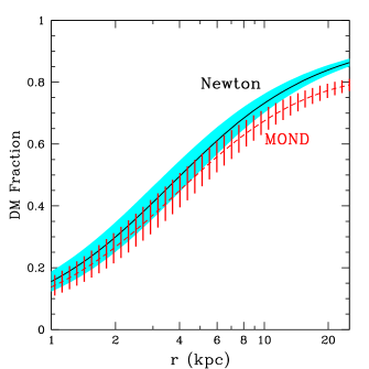
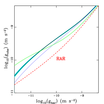
Figure 7.— (Left Panel) Radial profiles of the DM fraction within the central $\sim 25$ kpc for the fiducial HE model for the Newtonian (black and cyan) and MOND (red) cases. The shaded and hashed regions represent $1\sigma$ errors. (Right Panel) The solid black line enclosed by the cyan region shows the mean (i.e., “Best Fit”) and standard deviation of the posterior of the fiducial Bayesian HE model of Mrk 1216 for the radial gravitational acceleration $(g_{\rm obs})$ plotted versus the acceleration arising from only the baryonic mass components (i.e., stars+SMBH+gas). (Only the errors in $g_{\rm obs}$ are shown. The errors for $g_{\rm bar}$ are much smaller.) The blue dotted line is the “Best Fit” result for NGC 6482 computed using the corresponding fiducial HE model from B17. The dashed red line is the “universal” RAR of Lelli et al. (2017). The range plotted for $g_{\rm bar}$ corresponds to $1\leq R\leq 100.7$ kpc. The dotted green line is the “Best Fit” Bayesian HE model for Mrk 1216 with high-baryon mass and low central DM concentration (see §7.8 and §9.2).

We have also interpreted our HE analysis in terms of MOND (Milgrom 1983) to compare to our traditional Newtonian analysis. Our method follows Sanders (1999) and Angus et al. (2008) and is most recently described in detail in §6.7 of B17. In Figure 7 we display the DM fraction profile within a radius of 25 kpc for our fiducial Bayesian HE model computed from the Newtonian and MOND perspectives. As is clear in the figure, MOND requires almost as much DM as in the Newtonian approach, very similar to what we found for NGC 6482 (B17).

The MOND acceleration scale $a_{0}\approx 1.2\times 10^{-8}$ cm s^-2 is reached at a radius $\approx 11$ kpc (considering only the mass in baryons – stars+SMBH+gas, $\sim 42$ kpc otherwise). Even considering a much smaller central DM contribution (i.e., setting $c_{200}=10$ in the Newtonian analysis, too small to be consistent with the data – see §9.2) with correspondingly much larger stellar mass contribution (${M_{\star}/L_{H}}\sim 1.6$ solar) only changes this radius by $\sim 1$ kpc; i.e., the need for DM in MOND occurs well within the Newtonian regime of Mrk 1216. Hence, Mrk 1216 and NGC 6482 provide strong evidence that MOND requires DM on the massive galaxy scale, extending to lower masses the results obtained from HE studies on the group (e.g., Angus et al. 2008) and cluster (e.g., Pointecouteau & Silk 2005) scales.

Given the close similarity between MOND and the Radial Acceleration Relation (RAR, Lelli et al. 2017), it is also to be expected that these galaxies deviate significantly from the RAR. Indeed, as shown in Figure 7 we find that the gravitational acceleration we derive from our HE analysis $(g_{\rm obs})$ for Mrk 1216 (and NGC 6482) significantly exceeds the acceleration from only the baryons $g_{\rm bar}$. For example, at the MOND acceleration scale, $g_{\rm bar}=1.2\times 10^{-10}$ m s^-2, the RAR predicts $g_{\rm obs}=1.9\times 10^{-10}$ m s^-2 whereas we measure for Mrk 1216 $g_{\rm obs}=(4.99\pm 0.15)\times 10^{-10}$ m s^-2. Lelli et al. (2017) quote a scatter in the RAR of $\lesssim 0.13$ dex indicating at this one data point the discrepancy is $>3\sigma$. In fact, as seen in Figure 7 this level of discrepancy applies over a wide range in $g_{\rm bar}$, and thus the significance of the discrepancy with the entire RAR is in fact much larger.

Finally, we mention that in Figure 7 we also show $g_{\rm obs}$ for the $c_{200}=10$ model mentioned above which has a lower central DM and a higher baryon contribution for Mrk 1216. Although the shape of the $g_{\rm obs}$ profile is different from the fiducial model, the level of discrepancy with the RAR is broadly similar. The fractional errors (not shown) for $g_{\rm obs}$ of this model are similar to the fiducial model.

7.9. Gas and Baryon Fraction

Table 12Gas and Baryon Fraction

	$f_{\rm gas,2500}$	$f_{\rm b,2500}$	$f_{\rm gas,500}$	$f_{\rm b,500}$	$f_{\rm gas,200}$	$f_{\rm b,200}$
Best Fit	$0.028\pm 0.003$	$0.071\pm 0.006$	$0.058\pm 0.008$	$0.089\pm 0.010$	$0.094\pm 0.015$	$0.120\pm 0.016$
(Max Like)	$(0.027)$	$(0.071)$	$(0.058)$	$(0.089)$	$(0.094)$	$(0.120)$
1 Brk Entropy	$0.001$	$0.001$	$0.004$	$0.004$	$0.007$	$0.008$
BH Flat Prior	$0.000$	$0.000$	$0.001$	$0.001$	$0.002$	$0.002$
BH Flat Logspace Prior	$-0.000$	$0.001$	$-0.000$	$0.000$	$-0.000$	$0.000$
Fixed Over-Massive BH	$0.002$	$-0.010$	$0.007$	$-0.001$	$0.013$	$0.007$
Fixed ${M_{\rm BH}-\sigma}$ BH	$0.001$	$-0.002$	$0.002$	$0.000$	$0.004$	$0.002$
Sersic Stars 2MASS	$-0.001$	$-0.003$	$-0.004$	$-0.006$	$-0.008$	$-0.010$
Einasto	$-0.002$	$-0.009$	$-0.005$	$-0.010$	$-0.009$	$-0.012$
Strong AC	$-0.003$	$-0.022$	$-0.011$	$-0.025$	$-0.020$	$-0.033$
Weak AC	$-0.002$	$-0.008$	$-0.006$	$-0.011$	$-0.011$	$-0.015$
Weak AC Einasto	$-0.004$	$-0.016$	$-0.012$	$-0.022$	$-0.022$	$-0.031$
Joint Fit of Cycle 19 Obs.	$-0.000$	$0.001$	$0.001$	$0.002$	$0.003$	$0.004$
Constant $Z_{\alpha}/{Z_{\rm Fe}}$	$-0.001$	$0.002$	$-0.004$	$-0.002$	$-0.007$	$-0.005$
Annulus 10 $\Delta{Z_{\rm Fe}}$	${}^{+0.002}_{-0.002}$	${}^{+0.003}_{-0.004}$	${}^{+0.005}_{-0.006}$	${}^{+0.006}_{-0.007}$	${}^{+0.009}_{-0.010}$	${}^{+0.010}_{-0.011}$
Deproj	$0.010$	$0.007$	$0.023$	$0.022$	$0.040$	$0.038$
Distance	$0.003$	$0.006$	$0.005$	$0.007$	$0.007$	$0.008$

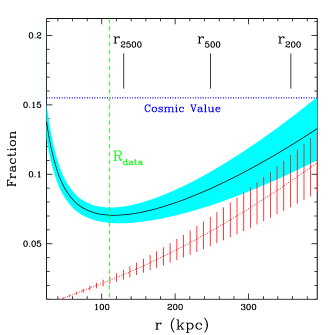
Figure 8.— Baryon fraction (solid black line, shaded cyan $1\sigma$ error region) and gas fraction (dotted red line, shaded red $1\sigma$ error region) of the fiducial Bayesian HE model. The green vertical dashed line indicates the outer extent of the Chandra data analyzed $(R_{\rm data})$.

We display the radial profiles of the gas $(f_{\rm gas})$ and baryon fractions $(f_{\rm b})$ in Figure 8 for the fiducial Bayesian HE model and list the results for these quantities within radii ${r_{2500}}$, ${r_{500}}$, and ${r_{200}}$ in Table 12 along with the systematic error budget. Within ${r_{2500}}$, which essentially represents the extent of the Chandra data, we measure $f_{\rm b,2500}=0.071\pm 0.006$; i.e., $\approx 45\%$ of the cosmic mean value $f_{\rm b,U}=0.155$ determined by Planck (Planck Collaboration et al. 2014), where the hot gas contributes $\approx 40\%$ of the measured baryons. The gas and baryon fractions continue to increase with radius until at ${r_{200}}$ we have $f_{\rm b,200}=0.120\pm 0.016$ comprising nearly $80\%$ of the comic mean. Here the hot gas contributes $\approx 80\%$ of the measured baryons.

Thus far we have only considered the stellar baryons associated with the MGE decomposition of the HST $H$-band light from Y17. Yıldırım et al. (2015) note there are only two galaxies known within a 1 Mpc radius of Mrk 1216. Using NED we identify these galaxies as 2MASX J08284832-0704316 (PGC152584) and 2MASX J08291551-0647454 (PGC152635), which on the sky are located, respectively, $\approx 220$ kpc ($\approx 0.9{r_{500}}$) and $\approx 300$ kpc ($\approx 0.9{r_{200}}$), from the center of Mrk 1216. There is sparse information on these galaxies. However, based on their 2MASS $K$-band magnitudes they are each about 2 magnitudes fainter than Mrk 1216, suggestive of a fossil group. If we assume a similar contribution of non-central baryons as for the fossil group NGC 6482, that would add $\approx 0.04$ to the baryon fraction at ${r_{200}}$ to give $f_{\rm b,200}\approx 0.16$, consistent with the cosmic mean value.

Most of the systematic errors we have considered (Table 12) shift the gas and baryon fractions by less than the statistical error. The spectral deprojection (“Deproj” test) shifts are not significant within the larger $1\sigma$ erros in the deprojection model; e.g., $1\sigma$ error is $\pm 0.041$ on $f_{\rm b,200}$. The AC models have the largest effect resulting in lower values. The Weak AC Einasto model, which is our favored model (see §9.1), yields $f_{\rm b,200}$ lower by 0.036 which effectively cancels the expected increase from non-central baryons.

We conclude that the Bayesian HE models predict that $f_{\rm b,200}$ is close to the cosmic mean value for Mrk 1216. In §9.4 we discuss this measurement in relation to previous X-ray studies of other fossil elliptical galaxies and consider the implications for the “Missing Baryons” problem.

7.10. Cooling Time and Free-Fall Time

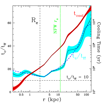
Figure 9.— Ratio of the cooling time $(t_{c})$ to the free-fall time $(t_{\rm ff})$ versus radius for the fiducial Bayesian HE model. The solid black line is the mean (i.e., “Best Fit”) and the associated cyan region is the standard deviation of the posterior. For comparison, we show with the dashed blue line the “Best-Fit” result for the model having only one break radius in the entropy profile (§7.1). The vertical black dashed line indicates the $H$-band stellar half light while the vertical green dotted line shows the “Best Fit” NFW scale radius $r_{s}$. The horizontal dashed black line shows the value $t_{c}/t_{\rm ff}=10$ proposed as an approximate lower limit before the onset of multiphase cooling (e.g., Sharma et al. 2012; Gaspari et al. 2012b; Meece et al. 2015). The corresponding cooling time is shown by the solid black line and associated red region with values plotted on the right vertical axes.

In Figure 9 we plot ${t_{\rm c}}/{t_{\rm ff}}$, the ratio of cooling time to free-fall time, as well as ${t_{\rm c}}$ itself, as a function of radius for the fiducial Bayesian HE model. Mrk 1216 displays a large central region of approximately constant ${t_{\rm c}}/{t_{\rm ff}}$; i.e., for $r\leq 10$ kpc, ${t_{\rm c}}/{t_{\rm ff}}\approx 14-19$. Outside of this region, ${t_{\rm c}}/{t_{\rm ff}}$ increases with radius. The ${t_{\rm c}}/{t_{\rm ff}}$ profile of Mrk 1216 resembles a scaled down version of the massive cluster Hydra-A (Hogan et al. 2017), which has pronounced X-ray cavities associated with AGN radio jets. Similarly, the observed ${t_{\rm c}}/{t_{\rm ff}}$ profile more closely resembles massive elliptical galaxies and groups with evidence for multiphase gas (see Figure 2 of Voit et al. 2015). The ${t_{\rm c}}/{t_{\rm ff}}$ profile suggests “precipitation-regulated AGN feedback” (e.g., Voit et al. 2017) for Mrk 1216, and we discuss further the implications of Mrk 1216 for feedback models in §9.5.

We also remark that the approximately constant region of ${t_{\rm c}}/{t_{\rm ff}}\approx 17$ ends near the NFW scale radius $r_{s}\approx 12$ kpc (and for ${t_{\rm c}}\approx 10^{8}$ yr) for the fiducial model. We obtain extremely similar ${t_{\rm c}}/{t_{\rm ff}}$ profiles for the Einasto DM model ($r_{s}\approx 14$ kpc) and other models (e.g., AC); i.e., in Mrk 1216 the DM scale radius approximately equals the feedback radius.

8. Error Budget

As in our previous studies we have examined the sensitivity of our measurements for the mass profile to various choices we have made in the spectral fitting and HE analysis. Many of these are listed in Tables 6 and 12 and have been discussed already in the text (e.g., SMBH priors, various DM and AC models), and we will not say anything further about them here. We mention that the numbers quoted for the systematic errors in Tables 6 and 12 are intended to provide the interested reader with some idea of how sensitive are the fiducial model parameters to arbitrary (but well motivated) changes to the fiducial model and/or analysis. As such, these numbers should not be added in quadrature to produce a single systematic error bar for a given parameter.

Below we provide more details for several tests in §8.1, §8.2, §8.3, and §8.6. First we very briefly list several notable tests that did not affect the measured HE model parameters significantly.

Entropy Profile: We examined an entropy profile with only a single break radius (see §7.1) with results listed in Tables 10 and 12 and the best-fitting model shown as the red dotted line in Figure 6. We also studied larger radii where the baseline gravity-only slope (see §5) sets in, $r_{\rm b,baseline}=250,500$ kpc.

Joint Spectral Fitting of Individual Cycle 19 Observations: We found no significant differences in the derived HE models when the gas properties of the Cycle 19 observation are obtained without summing the spectra of the individual exposures (§4.2.1, Appendix A, Tables 10 and 12).

Radial Extent of Models: By default we filled the gravitational potential of our HE models with hot gas out to a radius of $r_{\rm max}=1$ Mpc. We also examined $r_{\rm max}=0.5,1.5$ Mpc.

Soft CXB: We examined rescaling the nominal fluxes of the soft CXB components (§4.1) by factors of 0.5 and 2.

8.1. Choice of Center

As noted in §3.1, the centroid of the X-ray brightness changes by very little within the central $\sim 20\arcsec$. For our analysis we adopted the center position obtained by computing the centroid within a circle of radius $3\arcsec$ placed initially on the nominal stellar galaxy position. The annuli used for spectral extraction (Table 6) were defined about this centroid position (8:28:47.141,$-$6:56:24.367).

To gauge the sensitivity of our results to this choice, we also examined using the center position (8:28:47.131,-6:56:24.047) located at the emission peak $\approx 0.35\arcsec$ to the NW. Using this center has no measurable effect on the results.

8.2. Deprojection

In §4.2.2 we discussed the results obtained for the spectral fitting when using a deprojection analysis. One issue that requires clarification is the error bars reported in Table 15. Because of the correlations between annuli introduced by the deprojection procedure, we estimate errors on the gas parameters (temperature, normalization, and abundances) via Monte Carlo simulations in xspec as we have done in previous studies of deprojected spectra (e.g., Buote 2000a; Buote et al. 2003a); i.e., we performed 100 simulations of each set of spectra, computed the gas properties (e.g., temperature) for each simulation, and then compute the standard deviations on the parameters which we quote as the $1\sigma$ errors in Table 15.

For our analysis of the projected spectra we have also computed parameter errors by simply finding the values of a given parameter that change the C-statistic by 1 from its minimum value; i.e., using the error command in xspec. (We quote these results by default; e.g., Table 6). As expected, for the projected spectral analysis we find that both approaches – $\Delta C=1$ and Monte Carlo – give very consistent results.

As mentioned in §4.2.2, we performed deprojected spectral fits for two cases: (1) no gas emission was accounted for outside of the bounding annuli; (2) gas emission predicted by the Best Fit fiducial HE model from the projected spectral analysis (Table 8) was assigned to the large background apertures exterior to the bounding annuli. The results for case (2) are presented in the “Deproj” entries in Tables 10 and 12.

For most parameters the “Deproj” systematic test shifts the values by an amount comparable to the $1\sigma$ statistical error. As noted in §7.9, the listed positive shifts and the gas and baryon fractions are not statistically significant when considering the larger statistical uncertainties of the deprojection models. Case (1) produces larger shifts that are modestly significant; e.g., $f_{\rm b,200}$ is increased by $0.063\pm 0.038$. However, we prefer not to emphasize case (1) given that it does not account for emission projected into the bounding annuli. Finally, we also mention that the minimum $\chi^{2}$ achieved for the frequentist HE analysis for both deprojected cases is $\approx 8$ larger than the projected fit; i.e., the fits are formally acceptable for the deprojected cases, but the default projected analysis gives a better fit.

We conclude that the constraints on the mass profile obtained when using the spectral deprojection approach are overall very consistent with the default projection analysis.

8.3. Metal Abundances

When we do not allow the abundance ratios ${Z_{\rm Mg}/Z_{\rm Fe}}$ and ${Z_{\rm Si}/Z_{\rm Fe}}$ to vary with radius in the spectral fits (§4.2.1), the effects on the HE models are listed in the “Constant $Z_{\alpha}/{Z_{\rm Fe}}$” entries in Tables 10 and 12. This test shifts most of the parameters by an amount comparable to the $1\sigma$ errors and, in the case of ${M_{\star}/L_{H}}$, by $\approx 1.5\sigma$. Interestingly, the results for this test differ noticeably for the Best Fit and Max Like values. The shifts of marginal significance listed in the tables reflect only the Best Fit values. If we compare Max Like values instead, then all the shifts are $<1\sigma$.

When we allow ${Z_{\rm Fe}}$ to take values $0.27\,{Z_{\odot}}$ and $0.45\,{Z_{\odot}}$ for Annulus 10 of the Cycle 19 observation (see §4.2.1) representing the intrinsic scatter of the average group/cluster profile of Mernier et al. (2017), we list the parameter shifts for the HE models in the “Annulus 10 $\Delta{Z_{\rm Fe}}$” entries in Tables 10 and 12. All the quoted parameter shifts are less than the statistical errors.

8.4. Radial Range

Throughout the paper we have quoted global parameters (e.g., concentration, mass, etc.) for a series of “virial” radii representing three common overdensities; i.e., ${r_{2500}}$, ${r_{500}}$, and ${r_{200}}$ (see §7), where ${r_{2500}}$ essentially matches the radial extent of the Cycle 19 observation, while ${r_{500}}\approx 1.9{r_{2500}}$ and ${r_{200}}\approx 2.8{r_{2500}}$ fall outside the observed data range. Our analysis of the projected data technically constrains the projected emission for radii outside the data range in projection (i.e., $r>{r_{2500}}$). In reality, the emission from radii much larger than the data extent projected onto the observed sky annuli is dominated by the emission from within the three-dimensional spherical shells corresponding to the radii of the observed sky annuli. Hence, the global parameter values quoted at radiii ${r_{500}}$ and, particularly, ${r_{200}}$ are to an increasing amount extrapolations of our model outside the data range.

We do not expect significant systematic error in the extrapolated parameter values (e.g., $c_{200}$, and $M_{200}$) provided (1) the true DM profile is accurately described by the NFW/Einasto models and (2) we have accurately measured the DM scale radius $r_{s}$. Previously in Gastaldello et al. (2007) we emphasized that accurate and precise constraints on $r_{s}$, and thus the NFW DM profile, from HE X-ray studies are only possible when several radial data bins exist both above and below $r_{s}$. For Mrk 1216 we measure $r_{s}=12.1\pm 2.2$ kpc so that approximately 6 annuli lie below $r_{s}$ and 4 annuli above $r_{s}$ for the Cycle 19 data, with $R_{\rm out}\approx 9r_{s}$ where $R_{\rm out}=110.7$ kpc is the outer radius of Annulus 10. (The Cycle 16 data contribute 4 annuli below $r_{s}$, 2 annuli above $r_{s}$, and one annulus encloses $r_{s}$.) Since $r_{s}$ is situated well within the data range with several radial bins above and below it, we believe it is well constrained, as is reflected in the Bayesian constraints; e.g., for the fiducial HE model we obtain $r_{s}=12.1_{-4.4}^{+7.1}$ kpc (99% confidence).

It is instructive to consider the fossil cluster RXJ 1159+5531 for which the accuracy of some radial extrapolation (i.e., from ${r_{500}}$ to ${r_{200}}$) has been directly tested. Although it is $\approx 15$ more massive, RXJ 1159+5531 is similar to Mrk 1216 in that it is a highly relaxed system with an above-average halo concentration. Using a single Chandra observation with data extending out to $\approx{r_{500}}$ with approximately 5 (4) data bins below (above) $r_{s}$, Gastaldello et al. (2007) obtained $c_{200}=8.3\pm 2.1$ and $M_{200}=(7.9\pm 5)\times 10^{13}\,M_{\odot}$ with $r_{s}\approx 104$ kpc. Later, adding several Suzaku observations covering the entire sky region out to ${r_{200}}$, in Buote et al. (2016) we obtained $c_{200}=8.4\pm 1.0$ and $M_{200}=(7.9\pm 0.6)\times 10^{13}\,M_{\odot}$ with $r_{s}\approx 104$ kpc, extremely consistent with the previous extrapolated measurement. Notice in particular that $r_{s}$ did not change between the studies.

Based on a suite of cosmological hydrodynamical cluster simulations, Rasia et al. (2013) reported that significant positive biases (up to 25%) in the inferred value of $c_{200}$ are possible if the X-ray HE analysis only fits data within $\approx{r_{2500}}$. However, the largest biases occur for their simulations without AGN feedback. When AGN feedback is included, the bias is small (i.e., $\lesssim 10\%$, see Figure 5 of Rasia et al. 2013). The lowest mass clusters studied by Rasia et al. (2013) have $M_{200}\approx 2\times 10^{14}$; i.e., $\approx 40$ times more massive than Mrk 1216. Assuming these results apply to lower-mass halos like Mrk 1216, then the $\lesssim 10\%$ bias for the simulations with AGN feedback is comparable to or less than the statistical error we measure for Mrk 1216.

In a future paper we will test the extrapolation for Mrk 1216 using a new deep XMM-Newton observation that will extend the radial range of the model fits closer to ${r_{500}}$.

8.5. Spherical Symmetry

It has been shown that spherical averaging of an ellipsoidal mass profile typically introduces only small orientation-averaged biases for global quantities such as $c_{200}$, $M_{200}$, and $f_{\rm gas,200}$ in X-ray HE studies of galaxy and cluster masses (e.g., Buote & Humphrey 2012b, c, and references therein). Since we also found such small biases to be negligible compared to the statistical errors for the massive elliptical galaxy NGC 6482 (see B17), which has DM properties very similar to Mrk 1216, we do not present a specific estimate here.

We have also considered in this paper the mass profile near $R_{e}$. Previous studies of the spherical approximation in X-ray studies of galaxy clusters do not specifically address such a small radius. However, in Buote & Humphrey (2012b, see also ) we showed that spherically averaging an ellipsoidal scale-free logarithmic potential in a HE analysis introduces zero bias in the inferred mass for any gas temperature profile. We expect this result to apply to a good approximation near $R_{e}$ where it is well established that the total mass profile slope $\langle\gamma\rangle\approx 2$ for massive ETGs, as we have found for Mrk 1216 (see §7.7).

We can test this expectation for the massive elliptical galaxy NGC 720 for which we previously reported a value $M_{\rm tot}/L_{B}=6.0$ solar at $R_{e}$ obtained from spherically averaging ellipsoidal HE model fits to the Chandra data (Buote et al. 2002). We compare this measurement to the results of the fully spherical HE analysis of NGC 720 we performed using the same Chandra data in Humphrey et al. (2006) after accounting for the slightly different distance used and the fact the latter study quotes $M_{\rm tot}/L_{K}$; i.e., $M_{\rm tot}/L_{B}=6.0$ solar becomes $M_{\rm tot}/L_{K}=1.1$ solar in excellent agreement with the $M_{\rm tot}/L_{K}$ profile displayed in Figure 5 of Humphrey et al. (2006). We therefore expect that systematic errors associated with spherical averaging should also be small near $1R_{e}$ for Mrk 1216.

8.6. Stellar Mass Profile

To assess the sensitivity of our results to the shape of the stellar light profile, we also considered a de Vaucouleurs model (i.e., $n=4$ Sersic model) with the half-light radius inferred from the Two Micron All-Sky Survey (2MASS) Extended Source Catalog (Jarrett et al. 2000). We adopted a median, circularized $R_{e}=2.1$ kpc and normalized the model the total $H$-band luminosity (Table 2). We list the results for this test in the “Sersic Stars 2MASS” entries in Tables 10 and 12. In all cases using the Sersic model shifts the paramers by $\leq 1\sigma$.

9. Discussion

9.1. High Halo Concentration and Formation History

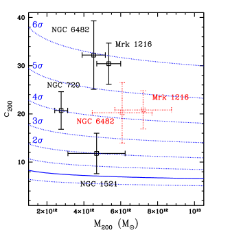
Figure 10.— Concentration and mass values for Mrk 1216, the fossil group NGC 6482, and two “nearly fossil” massive elliptical galaxies (see §9.1). The blue solid line is the $\Lambda$CDM relation for relaxed halos from Dutton & Macciò (2014) evaluated at the distance of Mrk 1216. The blue dotted lines indicate the intrinsic scatter in the $\Lambda$CDM relation; i.e., the lines closest the mean relation are $\pm 1\sigma$ while the significances of the other lines are indicated. The data points indicated by red dots are models with Einasto DM halos that have undergone “weak” adiabatic contraction following Dutton et al. (2015) (see §5). Note that for these Einasto models the deviation from the mean is less than indicated for the NFW models by roughly $1\sigma$.

Table 13Comparison to Theoretical $\Lambda$CDM $c_{200}-M_{200}$ Relations

	Mrk 1216		Dutton+14		Ludlow+16		Child+18
DM Profile	$M_{200}$	$c_{200}$	$\bar{c}_{200}$	$\Delta c_{200}$	$\bar{c}_{200}$	$\Delta c_{200}$	$\bar{c}_{200}$	$\Delta c_{200}$
NFW	$(5.3\pm 0.6)\times 10^{12}\,{M_{\odot}}$	$30.4\pm 4.3$	7.0	$5.8\sigma$	$\cdots$	$\cdots$	6.1	$(11.9\sigma,6.3\sigma)$
Weak AC NFW	$(6.1\pm 1.0)\times 10^{12}\,{M_{\odot}}$	$23.9\pm 4.1$	6.9	$4.9\sigma$	$\cdots$	$\cdots$	6.1	$(9.0\sigma,5.5\sigma)$
Einasto	$(5.8\pm 1.0)\times 10^{12}\,{M_{\odot}}$	$27.2\pm 4.3$	7.9	$4.1\sigma$	7.2	$4.5\sigma$	7.1	$(8.4\sigma,4.5\sigma)$
Weak AC Einasto	$(7.2\pm 1.5)\times 10^{12}\,{M_{\odot}}$	$20.8\pm 4.0$	7.7	$3.4\sigma$	7.1	$3.7\sigma$	7.0	$(6.1\sigma,3.7\sigma)$

In Table 13 we compare the halo concentration $(c_{200})$ and mass $(M_{200})$ we have measured for Mrk 1216  using the Bayesian HE models to some theoretical models of the $\Lambda$CDM $c_{200}-M_{200}$ relation from the literature. Our fiducial model with an NFW DM halo exceeds the median $\Lambda$CDM relation by $\sim 6\sigma$ in terms of the intrinsic scatter of the theoretical relations. The size of this discrepancy implies an outlier so extreme as to be inconsistent with the $\Lambda$CDM simulations. Indeed, from visual inspection of published catalogs of $c_{200}$ and $M_{200}$ values we do not see any $\Lambda$CDM halos consistent with the NFW values we have measured for Mrk 1216; e.g., Figure 16 of Dutton & Macciò (2014) and Figure 2 of Ragagnin et al. (2018).

When substituting the Einasto DM profile for NFW the value obtained for $c_{200}$ remains high, though the tension with $\Lambda$CDM is reduced modestly to $4.1-4.5\,\sigma$ (Table 13). The reduced tension for the Einasto model is attributed both to the smaller value of $c_{200}$ measured for Mrk 1216 and the larger theoretical intrinsic scatter compared to the NFW profile (0.13 dex, Dutton & Macciò 2014). Nevertheless, we do not see any $\Lambda$CDM halos consistent with the Einasto values we have measured for Mrk 1216 in the simulation results published by Benson et al. (2018, see their Figures 2 and 4). Adiabatic contraction lowers $c_{200}$ more and further lessens the tension with $\Lambda$CDM to a more modest, though still substantial, $3.4-3.7\,\sigma$.

In Figure 10 we plot the $c_{200}$ and $M_{200}$ values for Mrk 1216 and three fossil and nearly fossil systems with evidence for above-average concentrations: NGC 720 (Humphrey et al. 2011), NGC 1521 (Humphrey et al. 2012), and NGC 6482 (B17). We refer to NGC 720 and NGC 1521 as “nearly” fossil systems since within their projected virial radii they obey the fossil classification. NGC 6482 in particular displays $c_{200}$ and $M_{200}$ behavior extremely similar to Mrk 1216 – both in terms of its outlier status with respect to $\Lambda$CDM and the way the $c_{200}$ and $M_{200}$ parameters change between NFW, Einasto, and AC models.

The very high halo concentration we have measured for Mrk 1216 has profound implications for its formation and evolutionary history. The halo formation time is a major factor determining the scatter in halo concentrations for a given mass (e.g., Neto et al. 2007; Ludlow et al. 2016), with higher concentrations reflecting halos that have formed earlier. Consequently, the high value of $c_{200}$ indicates that, compared to the typical halo of its total mass, most of the mass of Mrk 1216 was in place much earlier, which is consistent with largely passive evolution for most of its existence. Thus the high concentration provides vital corroborating evidence of Mrk 1216 as a massive “relic galaxy” that is a largely untouched descendant of the red nugget population at high redshift (e.g., van den Bosch et al. 2015; Yıldırım et al. 2015; Ferré-Mateu et al. 2017; Yıldırım et al. 2017).

While the connection between early formation and high $c_{200}$ is critical, other factors must also contribute. Ludlow et al. (2016) estimate that formation time accounts for a large fraction ($\sim 50\%$) of the scatter in $c_{200}$, leaving about half the scatter to be likely explained by the initial conditions or the environment of a given halo. The recent study by Ragagnin et al. (2018) proposes that a measure of the “fossilness” of a halo can account for some of this scatter, though the proposed effect is too modest to explain the large $c_{200}$ of Mrk 1216. These issues are likely central to understanding how the DM and total mass profiles of Mrk 1216 and NGC 6482 are extremely similar yet the stellar component of Mrk 1216 is more compact obeying the size-mass relation for $z\sim 2$ galaxies like other CEGs.

Finally, we note that we have emphasized comparisons with the theoretical $c_{200}-M_{200}$ relations assuming a lognormal intrinsic scatter. While a gaussian interpretation of the theoretical scatter is consistent with cosmological simulations (e.g., Bhattacharya et al. 2013), the narrower tails of the gaussian imply Mrk 1216 would be an outlier so extreme (see Child+18 results in Table 13) for all models to be incompatible with $\Lambda$CDM. Consequently, the high $c_{200}$ values for Mrk 1216 and NGC 6482 (B17) clearly favor a lognormal distribution for the intrinsic scatter of the $\Lambda$CDM $c_{200}-M_{200}$ relation.

9.2. A Key Factor Contributing to Differences in the X-ray and Stellar Dynamical Constraints

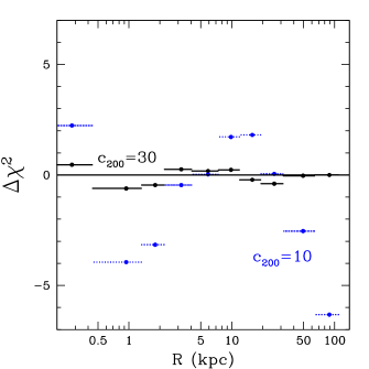
Figure 11.— $\chi^{2}$ residuals for frequentist HE model fits. We show only the surface brightness residuals for the Cycle 19 data. In black we show the fiducial model ($c_{200}=30$) while in blue we show the model with $c_{200}=10$, a value typically assumed in stellar dynamical studies that do not constrain the DM halo.

We have found significant differences in the mass properties of Mrk 1216 inferred from our HE analysis of the hot plasma within a radius $\sim R_{e}$ compared to the stellar dynamical (SD) constraints obtained by Y17 and Walsh et al. (2017). There is, however, a major difference in the assumed DM model between these SD studies and ours. Since the SD studies are unable to contrain the DM halo, by default they assume an NFW DM halo with fixed $c_{200}=10$. Here we consider how our HE analysis changes if we make a similar assumption.

We achieve a similar DM halo in our analysis by fixing the NFW scale radius to $r_{s}=60$ kpc in which case we obtain, $c_{200}=9.8\pm 0.2$ and $M_{200}=(2.3\pm 0.1)\times 10^{13}\,{M_{\odot}}$ from our Bayesian analysis. The fit quality, however, is very poor; i.e., the frequentist analysis gives $\chi^{2}=39.5$ for 19 dof compared to $\chi^{2}=11.9$ when $c_{200}=$ is allowed to take a value $c_{200}=30.$ In Figure 11 we plot the $\chi^{2}$ residuals for the $c_{200}\approx 10,30$ models, showing just the surface brightness data for the Cycle 19 observation. Compared to the $c_{200}=30$ model, the $c_{200}=10$ model has much larger residuals over most of the radial range; i.e., the Chandra data clearly exclude the $c_{200}=10$ model in favor of the $c_{200}=30$ model.

While the $c_{200}=10$ model does not provide a good fit to the data, the derived mass parameters agree very well with those of Y17. We obtain ${M_{\star}/L_{H}}=1.60\pm 0.05$ solar which agrees with Y17’s value, ${M_{\star}/L_{H}}=1.85^{+0.52}_{-0.40}$, within their larger $1\sigma$ error bar. While Y17 do not quote values of the total mass slope and DM fraction within $R_{e}$ specifically for Mrk 1216, their sample-averaged values ($\langle\gamma\rangle=2.3$, $f_{\rm DM}=0.11$) agree very well with what we obtain for Mrk 1216 ($\langle\gamma\rangle=2.27\pm 0.01$, $f_{\rm DM}=0.13\pm 0.01$) when we assume $c_{200}=10$. Furthermore, if we also fix the SMBH mass to the best-fitting “over-massive” value (${M_{\rm BH}}=4.9\times 10^{9}\,{M_{\odot}}$) obtained by Walsh et al. (2017), then we obtain an even worse fit ($\chi^{2}=50.3$ for 20 dof) but with ${M_{\star}/L_{H}}=1.36\pm 0.05$ solar in excellent agreement with the value ${M_{\star}/L_{H}}=1.3\pm 0.4$ solar obtained by Walsh et al. (2017).

We conclude that the assumption of $c_{200}=10$ for the NFW DM halo fully accounts for the higher ${M_{\star}/L_{H}}$ measured with SD by Y17 and Walsh et al. (2017) as well as the higher $\langle\gamma\rangle$ and lower $f_{\rm DM}$ within $R_{e}$ obtained by Y17. Differences in the form of the DM halo, however, have negligible impact on our constraints on ${M_{\rm BH}}$ which are manifested only in the central $1\arcsec$ aperture (i.e., Annulus 1 of the Cycle 19 data). Below in §9.3 we evaluate the SMBH constraint further and consider its implications.

9.3. Evidence for Over-Massive Black Hole

In §7.3 we show that the HE analysis does not favor the best-fitting over-massive SMBH $[{M_{\rm BH}}=(4.9\pm 1.7)\times 10^{9}\,{M_{\odot}}]$ found by the SD study of Walsh et al. (2017), but does not clearly exclude the value either when considering different Bayesian priors and the frequentist fits. In addition, the SD error estimate on ${M_{\rm BH}}$ permits lower values (e.g., $1.4\times 10^{9}\,{M_{\odot}}\,(2\sigma)$ and $0.65\times 10^{9}\,{M_{\odot}}\,(2.5\sigma)$) that are very consistent with our HE models. In sum, the estimated statistical and systematic errors in the X-ray HE and SD constraints allow for broad consistency and do not clearly point to whether the SMBH exceeds the ${M_{\rm BH}-\sigma}$ relation.

Based on models of the Cycle 16 data of Mrk 1216 assuming ${M_{\rm BH}}=4.9\times 10^{9}\,{M_{\odot}}$, we expected to measure a value of ${k_{\rm B}T}$ about $20\%$ higher in Annulus 1 than we found with the Cycle 19 observation (see beginning of §7.3). If we attribute this underestimate to deviations from HE, it would imply $\sim 40\%$ non-thermal pressure support in Annulus 1 from random turbulent motions, magnetic fields, rotational support, etc. Future observations with similar or better spatial resolution to Chandra but with much higher spectral resolution and sensitivity (i.e, Lynx) will be necessary to establish the hot gas kinematics within the central $\approx 1\arcsec$. In the meantime, more precise constraints on ${M_{\rm BH}}$ from SD can better establish the significance of any tension with the X-ray constraints.

9.4. Global Baryon Fraction

Our Bayesian HE models evaluated at ${r_{200}}$ indicate $f_{\rm b,200}\approx 80\%$ of the cosmic mean value (§7.9). The evidence for near baryonic closure in Mrk 1216 is consistent with results we have obtained previously for other fossil-like massive elliptical galaxies, NGC 720 (Humphrey et al. 2011), NGC 1521 (Humphrey et al. 2012), and NGC 6482 (B17). These results suggest that in massive elliptical galaxy / small group halos many of the “missing” baryons (Fukugita et al. 1998) can be located in the outer halo as part of the hot component.

As is clear from Figure 8, most of the baryons inferred from our HE models within a radius of ${r_{200}}$ are in the form of hot gas located at radii larger than the extent of the Chandra data ($\gtrsim{r_{2500}}$). We have previously noted (§8.2 of B17) the sensitivity of the measured $f_{\rm gas,200}$ to the assumed value of ${Z_{\rm Fe}}$ for $r>{r_{2500}}$. In fact, using a $\beta$-model analysis of the Chandra surface brightness profile of NGC 720, Anderson & Bregman (2014) claim that the gas mass $(M_{\rm gas,200})$ is a factor 3-4 smaller than we measured in Humphrey et al. (2011).

We have reanalyzed the Chandra surface brightness profiles using all presently available observations and performed a similar $\beta$ model analysis of NGC 720. We find $M_{\rm gas,200}$ values very consistent with those of Humphrey et al. (2011). We attribute the lower value of $M_{\rm gas,200}$ obtained by Anderson & Bregman (2014) to primarily (1) their quoting a higher value of $M_{\rm gas,200}$ than was actually reported in Figure 6 of Humphrey et al. (2011); i.e., $4\times 10^{11}\,{M_{\odot}}$ instead of the correct $3\times 10^{11}\,{M_{\odot}}$ at $r=300$ kpc; (2) their using a different solar abundance standard (Anders & Grevesse 1989) whereas Humphrey et al. (2011) use Asplund et al. (2006); and (3) their assuming ${k_{\rm B}T}=0.5$ keV, ${Z_{\rm Fe}}=0.6$ solar for the hot plasma appropriate for the center of NGC 720 instead of quantities appropriate near ${r_{2500}}$ (${k_{\rm B}T}\approx 0.3$ keV, ${Z_{\rm Fe}}\approx 0.3$ solar).

To verify the nearly cosmic baryon fractions in these galaxies it is necessary to measure both ${k_{\rm B}T}$ and ${Z_{\rm Fe}}$ out to radii beyond ${r_{2500}}$. In future papers we will report the results of new deep XMM-Newton observations of Mrk 1216 and NGC 6482 that will allow the gas to be mapped out closer to $\sim{r_{500}}$.

9.5. Cooling and Feedback

The Chandra observations of Mrk 1216 suggest the hot plasma properties within the central $\sim 10$ kpc reflect a balance between radiative cooling and episodes of gentle AGN feedback. The centrally peaked radial temperature profile itself (Figure 5) does not implicate AGN shock-heating of the gas, since the continuous injection of stellar material will produce the same effect (e.g., classical wind models, David et al. 1991; Ciotti et al. 1991) and the observed central entropy is not peaked (Figure 6). Modern models of massive elliptical galaxies incorporating gentle mechanical AGN feedback episodes can produce similar centrally peaked temperature profiles (e.g., Gaspari et al. 2012a). The lack of large, significant disturbances (e.g., cavities) near the center (§3) or azimuthal spectral variations (§4.2.3) provides further evidence that episodic AGN feedback in Mrk 1216 has been gentle.

Interior to the sizable radius $\sim 10$ kpc within which ${t_{\rm c}}/{t_{\rm ff}}$ ranges from 14-19 (Figure 9, see §7.10), the “precipitation-regulated feedback” scenario (e.g., Voit et al. 2017) predicts there should be multiphase gas, yet there is little evidence presently for gas cooler than the ambient hot plasma. However, Voit et al. (2017) emphasizes that condensation will be suppressed by buoyancy damping if the entropy profile is steeply rising and without a large isentropic core. We find the entropy profile has a radial logarithmic slope $\alpha=0.78\pm 0.05$ for $0.66<r<16$ kpc (Table 8) and no evidence of a core. This slope is larger than the critical value $\alpha_{K}=2/3$ for suppressing condensation derived by Voit et al. (2017) using a toy model for isothermal gas.

In fact, this result may be common for massive, X-ray luminous elliptical galaxies. While the recent study by Babyk et al. (2018) finds a universal entropy profile for elliptical galaxies and galaxy clusters with an entropy slope consistent with $2/3$ within $0.1{r_{2500}}$, our previous measurements within the central $\sim 10$ kpc of massive elliptical galaxies have obtained steeper slopes $\alpha\gtrsim 1$ consistent with suppressed condensation: NGC 4649 (Humphrey et al. 2008), NGC 1332, NGC 4261, NGC 4472 (Humphrey et al. 2009a), and NGC 6482 (B17).

Although the $\alpha_{K}=2/3$ criterion for suppressing condensation from the toy model of Voit et al. (2017) is consistent with the single-phase gas we observe in Mrk 1216, the three-dimensional hydrodynamical simulations of Wang et al. (2018) predict that ${t_{\rm c}}/{t_{\rm ff}}$ should rise rapidly with radius for a single-phase gas, in conflict with the Chandra data (Figure 9) and the lack of evidence for multiphase gas in the amounts seen in other galaxies with ${t_{\rm c}}/{t_{\rm ff}}<20$ (Werner et al. 2014; Voit et al. 2015).

In §7.10 we remarked that the region where ${t_{\rm c}}/{t_{\rm ff}}$ ranges from 14-19 (i.e., $r\lesssim 10$ kpc), associated with a steeply rising entropy profile with $\alpha>2/3$, also is close to the NFW DM scale radius $r_{s}$. For the galaxies listed above with good constraints on the DM halo, $r_{s}$ is not far from 10 kpc; i.e., $r_{s}\approx 14$ kpc for NGC 720 and $r_{s}=11.2\pm 3$ kpc for NGC 6482.

We conclude by noting that the unusually quiescent evolutionary path indicated by the highly concentrated stellar and DM components of Mrk 1216 imply the presumed episodic AGN feedback regulating the cooling in the central $\sim 10$ kpc has not been upset by triggering from galaxy merging but has been solely governed by accretion from the radiatively cooling hot plasma. We speculate this has also resulted in unusually quiescent evolution in the hot plasma obeying the HE condition accurately (see below in §9.6).

9.6. Hydrostatic Equilibrium Approximation

Since the Chandra ACIS spectral data do not permit useful direct measurements of the kinematics of the hot plasma, we instead briefly summarize several indirect lines of evidence testifying to the accuracy of the HE approximation in Mrk 1216.

Azimuthal Scatter in Quadrants (§4.2.3) : When Annuli 2,3, and 4 of the Cycle 19 observations are divided up into quadrants, we find the small scatter of the pseudo-pressure and pseudo-entropy between quadrants in each annulus suggests HE deviations of $\lesssim 5\%$.

Quality of HE Model Fits (Table 9): We find that reasonable HE models provide excellent fits to the radial ${k_{\rm B}T}$ and ${\Sigma_{\rm x}}$ profiles of the Cycle 19 and Cycle 16 Chandra data.

Qualified Consistency with Stellar Dynamics Measurements (§9.2): If we fix $c_{200}=10$ for the NFW DM halo as done in the stellar dynamical studies by Y17 and Walsh et al. (2017), we find excellent agreement with the measured ${M_{\star}/L_{H}}$ values as well as the total mass slope ($\langle\gamma\rangle$) and DM fraction ($f_{\rm DM}$) obtained within $1R_{e}$. The constraints on ${M_{\rm BH}}$ are uncertain and therefore ambiguous with respect to the status of HE in Annulus 1 of the Cycle 19 data (§9.3).

Stellar Mass-to-Light Ratio and SPS Models (§7.4): The value we measure for ${M_{\star}/L_{H}}$ agrees very well with SPS models with a Kroupa IMF.

High Halo Concentration (§9.1): The exceptionally high value of $c_{200}$ we measure for Mrk 1216 corroborates the evidence from its compact stellar size and old stellar population that it is a massive relic galaxy; i.e., Mrk 1216 has evolved passively in isolation since a redshift of $\sim 2$ and, consequently, is highly evolved and relaxed.

We therefore expect that Mrk 1216 is a highly relaxed system, at least as relaxed as the massive Perseus cluster with its pronounced cavities and other surface brightness irregularities for which Hitomi found with gas kinematics measurements that the pressure from turbulence is only $4\%$ of the thermal gas pressure (Hitomi Collaboration et al. 2016). To verify directly the accuracy of the HE approximation in Mrk 1216 awaits the next generation of X-ray satellites with microcalorimeter detectors.

10. Conclusions

We present a detailed analysis of the hot plasma X-ray emission and gravitating mass profile of the CEG Mrk 1216 based on a new $\sim 122$ ks Chandra X-ray observation (Cycle 19) and a shallow ($\sim 13$ ks) archival Chandra observation (Cycle 16). The X-ray emission as revealed by the deep Cycle 19 image exhibits a regular, relaxed morphology symmetrically distributed about the central emission peak. We perform a detailed analysis of the image morphology within the central $\sim 15$ kpc to search for signs of AGN feedback. While the image does not reveal obvious features of AGN feedback in the form of cavities or other irregularities, we identify leading candidates for such feedback signatures as regions with the largest surface brightness fluctuations with respect to a smooth two-dimensional model.

We search for azimuthal variations in the gas pressure and entropy within the central $\sim 4$ kpc by dividing up several circular annuli into four quadrants each. Using proxies for the pressure and entropy inferred directly from the projected spectra, we find small azimuthal scatter in these proxies consistent with $\lesssim 5\%$ fluctuations in HE. Adopting an entropy-based HE method, we then place constraints on the inner and global mass profile from the radial profiles of temperature and surface brightness measured from spectra extracted in circular annuli extending out to $R=100.7$ kpc $(\approx 0.85{r_{2500}})$. (In Appendix C we discuss an anomalous spectral feature in the central $\approx 1\arcsec$ annulus.)

Our principal conclusion is that the halo concentration of Mrk 1216 is a large, positive outlier in the $\Lambda$CDM $c_{200}-M_{200}$ relation. For an NFW DM halo we obtain $c_{200}=30.4\pm 4.3$ and $M_{200}=(5.3\pm 0.6)\times 10^{12}\,{M_{\odot}}$ representing an extreme outlier in the $\Lambda$CDM $c_{200}-M_{200}$ relation; i.e., $\approx 6\sigma$ above the median theoretical value $c_{200}\approx 7$ (Table 13) considering the intrinsic scatter and $\approx 5.4\sigma$ considering the measurement error. If we replace the NFW DM profile with the Einasto profile modified by “weak” adiabatic contraction, the concentration is reduced to a less extreme (but still significant) $3.4-3.7\,\sigma$ outlier more compatible with $\Lambda$CDM.

The high value of $c_{200}$ we measure implies an unusually early formation time for Mrk 1216 and therefore a more passive and quiescent evolution compared to the typical halo. It therefore provides new independent evidence corroborating Mrk 1216 as a massive “relic galaxy” that is a largely untouched descendant of the red nugget population at high redshift. Moreover, whereas the stellar-mass-size relation and old stellar populations previously established the relic nature of the stellar component of CEGs, the high $c_{200}$ now firmly establishes the relic nature of the DM halo in Mrk 1216.

The high concentration of DM significantly affects the inferred mass properties near $R_{e}$. We measure a DM fraction $(f_{\rm DM})$ within $R_{e}$ about twice as large and a flatter total mass slope $(\langle\gamma\rangle)$ compared to local massive elliptical galaxies. Our measured values of $f_{\rm DM}$ and $\langle\gamma\rangle$ also disagree significantly with the mean values of the CEG sample (which includes Mrk 1216) by Y17. However, we attribute the discrepancy with Y17 to their assuming a fixed $c_{200}=10$ in their stellar dynamical analysis. If we assume $c_{200}=10$ in our HE analysis of the Chandra data, the fits are poor, but the parameters we derive agree very well with those reported by Y17. We conclude that if the other CEGs in Y17’s sample also have high $c_{200}$ values like Mrk 1216, then the sample-average values for $f_{\rm DM}$ and $\langle\gamma\rangle$ obtained by Y17 will need to be revised accordingly. Finally, if Mrk 1216 is truly a nearby analog of a $z\approx 2$ galaxy, the DM fraction we measure is larger than that produced in recent cosmological simulations of $z=2$ galaxies (§7.7).

If we instead interpret our results using MOND gravity, we find that MOND requires almost as much DM as in our Newtonian analysis. Owing to the strong similarity between MOND and the RAR, it would be expected that Mrk 1216 would deviate significantly from the RAR, which we verify. We attribute the failure of MOND and the RAR to explain the gravitational field of Mrk 1216 to the evidence for highly concentrated DM occurring well inside the radius where the gravitational acceleration equals the MOND constant $a_{0}$; i.e., the evidence for the DM is safely in the Newtonian regime not addressed by MOND. Although we have not explored other modified gravity models like self-interacting DM (SIDM) that predict DM cores, we believe it is likely that the highly concentrated DM in Mrk 1216 will place interesting constraints on DM models that predict inner halo profiles shallower than NFW.

Our analysis of the Chandra data does not place tight constraints on the SMBH mass, although our HE models do not favor the over-massive value $[{M_{\rm BH}}=(4.9\pm 1.7)\times 10^{9}\,{M_{\odot}}]$ obtained with stellar dynamics by Walsh et al. (2017). However, the tension between the X-ray and SD values of ${M_{\rm BH}}$ is modest considering the uncertainties in both measurements.

Within the extent of the Chandra data ($\approx{r_{2500}}$) we measure a baryon fraction $f_{\rm b,2500}=0.071\pm 0.006\approx 0.45f_{\rm b,U}$ with the hot gas contributing $\approx 40\%$ of $f_{\rm b,2500}$. When evaluating our models at ${r_{200}}$ we obtain $f_{\rm b,200}=0.120\pm 0.016\approx 0.80f_{\rm b,U}$ with $f_{\rm gas,200}\approx 0.8f_{\rm b,200}$; i.e., our analysis of the hot plasma indicates the halo of Mrk 1216 contains close to the cosmic fraction of baryons, where most of the baryons are in the form of hot plasma between ${r_{2500}}$ and ${r_{200}}$.

The radial profile of the ratio of cooling time to free-fall time varies within a narrow range $({t_{\rm c}}/{t_{\rm ff}}\approx 14-19)$ over a large central region ($r\leq 10$ kpc) exterior to which it increases with radius. The observed minimum ${t_{\rm c}}/{t_{\rm ff}}$ suggests “precipitation-regulated AGN feedback” for a multiphase plasma. There is presently little evidence for substantial amounts of multiphase gas within $r\sim 10$ kpc for Mrk 1216, which may indicate the steep radially increasing entropy profile has suppressed condensation of the hot plasma (see §9.5). We observe that the approximately constant region of ${t_{\rm c}}/{t_{\rm ff}}\approx 17$ ends near the NFW DM halo scale radius $r_{s}\approx 12$ kpc.

Finally, other than the compact size of the stellar half-light radius of Mrk 1216, the stellar, gas, and DM properties of Mrk 1216 are remarkably similar to those of the nearby fossil group NGC 6482 (B17). In particular, consideration of the nearly identical very high $c_{200}$ values for each, but different compactness of their stellar components, provides a striking example of factors other than formation time that must also contribute to the scatter in the $c_{200}-M_{200}$ relation; e.g., “fossilness” (Ragagnin et al. 2018).

Appendix A Joint Spectral Fitting of Individual Cycle 19 Observations

Table 14Hot Gas Properties from Joint fit of Cycle 19 Observations

		$R_{\rm in}$	$R_{\rm out}$	$\Sigma_{\rm x}$ (0.5-7.0 keV)	$k_{B}T$	$Z_{\rm Fe}$	$Z_{\rm Mg}/Z_{\rm Fe}$	$Z_{\rm Si}/Z_{\rm Fe}$
Telescope	Annulus	(kpc)	(kpc)	(ergs cm2 s-1 arcmin-2)	(keV)	(solar)	(solar)	(solar)
	1	0.00	0.44	$\rm 4.65e-11\pm 1.32e-11$	$0.971\pm 0.027$	$0.99\pm 0.17$	$1.54\pm 0.42$	$1.52\pm 0.31$
	2	0.44	1.33	$\rm 1.43e-11\pm 1.92e-12$	$0.904\pm 0.019$	$0.95\pm 0.09$	$1.10\pm 0.15$	$0.75\pm 0.08$
	3	1.33	2.21	$\rm 6.25e-12\pm 8.67e-13$	$0.841\pm 0.019$	$0.95\pm 0.08$	tied	tied
	4	2.21	4.10	$\rm 2.12e-12\pm 2.26e-13$	$0.814\pm 0.016$	$0.89\pm 0.06$	$0.81\pm 0.11$	tied
	5	4.10	7.42	$\rm 7.77e-13\pm 8.68e-14$	$0.733\pm 0.017$	$0.76\pm 0.05$	tied	tied
	6	7.42	11.96	$\rm 2.92e-13\pm 5.03e-14$	$0.665\pm 0.018$	$0.78\pm 0.08$	$0.54\pm 0.10$	$1.38\pm 0.13$
	7	11.96	19.26	$\rm 1.19e-13\pm 2.25e-14$	$0.668\pm 0.020$	$0.71\pm 0.07$	tied	tied
	8	19.26	31.77	$\rm 4.27e-14\pm 1.06e-14$	$0.680\pm 0.024$	$0.77\pm 0.09$	$0.81\pm 0.15$	tied
	9	31.77	64.20	$\rm 1.14e-14\pm 2.49e-15$	$0.616\pm 0.026$	tied	tied	tied
	10	64.20	110.70	$\rm 2.66e-15\pm 6.91e-16$	$0.689\pm 0.090$	0.36	tied	tied

In Table 14 we list the results for the gas properties obtained by jointly fitting the individual Cycle 19 exposures. The value of the C-statistic for the fit is 6487.8 for 6869 pha bins and 6799 dof. Note for this analysis the spectra of the individual exposures were rebinned in the same way as the combined spectra (§4).

Appendix B Spectral Deprojection Results

Table 15Hot Gas Properties Obtained from Spectral Deprojection

		$R_{\rm in}$	$R_{\rm out}$	$\rho_{\rm gas}$	$k_{B}T$	$Z_{\rm Fe}$	$Z_{\rm Mg}/Z_{\rm Fe}$	$Z_{\rm Si}/Z_{\rm Fe}$
Telescope	Annulus	(kpc)	(kpc)	(g cm-3)	(keV)	(solar)	(solar)	(solar)
Chandra Cycle 19
	1	0.00	0.44	7.76e-25 $\pm$ 1.94e-25	$0.988\pm 0.046$	$1.04\pm 0.30$	$1.85\pm 1.05$	$2.03\pm 0.85$
	2	0.44	1.33	2.58e-25 $\pm$ 3.01e-26	$0.954\pm 0.038$	$1.04\pm 0.18$	$1.24\pm 0.32$	$0.74\pm 0.15$
	3	1.33	2.21	1.81e-25 $\pm$ 2.28e-26	$0.841\pm 0.034$	$0.95\pm 0.16$	tied	tied
	4	2.21	4.10	6.75e-26 $\pm$ 8.04e-27	$0.850\pm 0.029$	$1.02\pm 0.16$	$0.91\pm 0.24$	tied
	5	4.10	7.42	3.62e-26 $\pm$ 3.94e-27	$0.740\pm 0.038$	$0.74\pm 0.11$	tied	tied
	6	7.42	11.96	1.56e-26 $\pm$ 2.11e-27	$0.716\pm 0.036$	$0.93\pm 0.15$	$0.55\pm 0.21$	$1.42\pm 0.20$
	7	11.96	19.26	1.03e-26 $\pm$ 1.55e-27	$0.617\pm 0.044$	$0.65\pm 0.13$	tied	tied
	8	19.26	31.77	4.17e-27 $\pm$ 4.69e-28	$0.717\pm 0.036$	$0.83\pm 0.13$	$0.78\pm 0.21$	tied
	9	31.77	64.20	1.58e-27 $\pm$ 1.93e-28	$0.601\pm 0.043$	tied	tied	tied
	10	64.20	110.70	9.45e-28 $\pm$ 1.80e-28	$0.677\pm 0.156$	0.36	tied	tied
Chandra Cycle 16
	1	0.00	0.78	5.21e-25 $\pm$ 7.85e-26	$1.232\pm 0.113$	$1.16\pm 0.29$	$0.60\pm 0.29$	$0.74\pm 0.32$
	2	0.78	1.77	1.94e-25 $\pm$ 3.27e-26	$0.829\pm 0.060$	tied	tied	tied
	3	1.77	3.54	7.00e-26 $\pm$ 1.30e-26	$0.852\pm 0.066$	tied	tied	tied
	4	3.54	6.86	3.99e-26 $\pm$ 6.48e-27	$0.763\pm 0.062$	$0.84\pm 0.17$	tied	tied
	5	6.86	14.39	1.46e-26 $\pm$ 2.34e-27	$0.640\pm 0.056$	tied	tied	tied
	6	14.39	28.78	5.95e-27 $\pm$ 9.38e-28	$0.767\pm 0.068$	$0.69\pm 0.14$	tied	tied
	7	28.78	73.06	1.49e-27 $\pm$ 2.80e-28	$0.611\pm 0.086$	tied	tied	tied

In Table 14 we list the results for the gas properties obtained for spectral projection using the projct model in xspec (§4.2.2).

Appendix C Anomalous Line Feature in the Central Spectrum of the Cycle 19 Observation

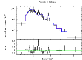
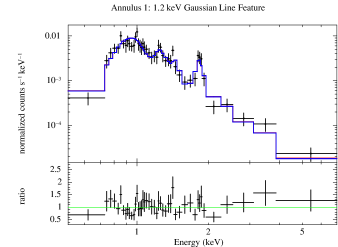
Figure 12.— Left panel:The Cycle 19 spectrum of Annulus 1 plotted as in Figure 4 except that the residuals are now shown in the bottom panel as data/model ratios. Right panel: A narrow gaussian emission line with $E\approx 1.23$ keV is added to improve the fit.

As noted in §4.2, the Cycle 19 spectrum of Annulus 1 displays some features that deviate from our adopted composite model, particularly an excess near $E\sim 1.2$ keV. Here we examine the fit residuals more closely and examine ways to improve the model fit. In the left panel of Figure 12 we again plot the spectrum and best-fitting model of Annulus 1 as in Figure 4 except now we also plot the data / model ratio in the bottom panel. Despite the presence of these residuals, the fit is marginally acceptable when judged by the value of the C-statistic or $\chi^{2}$; e.g., we obtain a $\chi^{2}$ null hypothesis probability of 2.5% if we consider only the Annulus 1 spectrum and ignore the negligible background but allow the 7.3 keV bremsstrahlung component normalization to vary freely (with the spectrum rebinned to at least 20 counts per channel).

To see if this marginal fit can be improved, we begin by considering well-motivated missing ingredients from our fiducial model. First, this single-temperature hot plasma component only approximates what is surely a continuous, radially varying temperature gradient within the aperture. We therefore expect emission from a range of temperatures which will produce a slightly broader thermal spectrum than our single-temperature model. In fact, the residuals displayed in Figure 12 resemble the residual pattern characteristic of fitting a single-temperature model to a multi-temperature spectrum with average ${k_{\rm B}T}\sim 1$ keV at ASCA/Chandra CCD resolution (e.g., Buote & Fabian 1998; Buote 2000b; Buote et al. 2003b). However, we are unable to improve the fit by adding more discrete temperature components or a continuous temperature distribution represented by, e.g., a gaussian differential emission measure. Spectral deprojection does not improve the fit either (§4.2.2). (We also found no improvement from models allowing for non-equilibrium ionization and plasma shocks.)

Second, the weak central radio source implies the presence of a low-luminosity AGN, and we might reasonably expect corresponding X-ray emission in the Chandra bandpass provided the AGN is not too heavily absorbed. As is readily apparent from Figure 12, there is no significant excess emission at higher energies signaling this component; i.e., the emission from the unresolved LMXB component is sufficient to describe the higher energies.

Since neither of these physically well-motivated modifications to the fiducial model obviously improves the fit, we resort to an empirical approach. The largest residual excess occurs near an energy 1.2 keV, and we are unable to adjust our fiducial model (including allowing other metal abundances to vary) to describe the feature. Consequently, we tried adding a narrow gaussian emission line and show the best-fitting result in the right panel of Figure 12. The fit is clearly improved, not only near the line, but for many of the energy channels below $\sim 1.5$ keV, with a reduction in the C-statistic of $\approx 19$.

We obtain good constraints on the fitted parameters of the line: energy, $E=1.231\pm 0.014$ keV, and flux, $\log_{10}F_{\rm x}=-14.83^{+0.10}_{-0.13}$ (with the $0.5-10$ keV flux in ergs cm^-2 s^-1), where the $3\sigma$ lower limit on the flux is $\log_{10}F_{\rm x}=-15.33$. Expressing the result in terms of the line luminosity, we obtain, $\log_{10}L_{\rm x}=-39.23^{+0.10}_{-0.12}$ (with luminosity in ergs s^-1).

We offer several possible explanations for this line feature and assess their validity.

(1) Problem with averaging the response matrices: Our default procedure combines the spectra from the four Cycle 19 exposures and averages the RMF and ARF files. However, we also perform the analysis through joint analysis of the individual observations and obtain fully consistent results.

(2) Calibration problem: We do not believe a calibration error is a viable explanation since we do not see this line feature in the spectra of the other annuli, nor are we aware of any reports of anomalous features in the ACIS-S near 1.2 keV.

(3) Plasma code: Since the available plasma codes exhibit some notable differences (e.g., Mernier et al. 2018), we compared our results using the vapec plasma code to those obtained with the cie plasma code from the spex v3.0 spectral fitting package (Kaastra et al. 1996). The cie model fit and resulting residual pattern is extremely similar to what we obtained with vapec. In particular, the cie model cannot explain the 1.2 keV line feature using parameters consistent with our fiducial vapec model. However, the cie model also allows for a variable Na abundance which can reproduce the 1.2 keV line feature reasonably well but only with a large, unphysical abundance ($>100$ solar).

(4) Decaying Dark Matter: X-ray emission lines may be signatures of decaying dark matter from a sterile neutrino (e.g., Abazajian 2017; Aharonian et al. 2017). The line flux we measure for the 1.2 keV feature is too strong and implies a mixing angle that is too large to be compatible with the currently allowed parameter space (e.g., Abazajian 2017).

(5) Charge exchange. The potential importance of charge exchange emission in clusters has been discussed, though observational evidence for it remains tentative (e.g., Gu et al. 2018a, b, and references therein). With spex we examined whether the charge-exchange model (CX) of Gu et al. (2016) could explain the line feature. The cx model can produce a Ne line at the right energy. However, along with 1.2 keV emission, the CX model produces considerably more Ne Ly$\alpha$ emission near 1 keV that is incompatible with the observation. In addition, the emission near 1.2 keV predicted by the CX model is broader than the observed feature.

In sum, none of the possibilities we have discussed is likely entirely responsible for the 1.2 keV line, and perhaps the feature is merely a statistical fluke. We believe, however, that the charge-exchange model deserves further study. First, the Ne line it predicts lies at the right energy. Second, for charge exchange to occur, there must be neutral material. Inspection of the residuals in the right panel of Figure 12 reveals that the lowest energies still show a deficit with respect to the model. When allowing for absorption in excess of the foreground Galactic absorbing column, the fit is improved a little more (C-statistic decreases by $\approx 4$) and is consistent with the presence of cold gas in the center. (Allowing the column density to be a free parameter in the other annuli produces no such improvement in the fit; i.e., the Galactic column is obtained elsewhere.) Although there is presently no direct evidence for neutral gas at the center of Mrk 1216, future observations with ALMA could determine whether a substantial amount of molecular gas surrounds the SMBH.

With our empirical approach here, we mention that adding the narrow gaussian has some effect on the parameters derived for the hot plasma component in Annulus 1. While we find ${k_{\rm B}T}$ is unaffected, $Z_{\rm Fe}$ increases and the gas density decreases. As a systemetics check on our fiducial results, we have used these modified gas parameters as input to our HE models and find that the main results are unchanged within the $\approx 1\sigma$ errors.

Finally, we also mention that in our brief use of the cie plasma model with spex in this section, we notice that the derived temperatures are typically 5-10 percent smaller than those obtained with the vapec model in xspec. We would expect this shift to translate to a similar reduction in magnitude for the masses we obtained from our HE models, which is comparable to the sizes of the $1\sigma$ statistical errors (Table 10) and of similar magnitude to other systematic errors considered. Fully interpreting all the data with spex for comparison to vapec is beyond the scope of our paper.

References

- Abazajian (2017) Abazajian, K. N. 2017, Phys. Rep., 711, 1
- Aharonian et al. (2017) Aharonian, F. A., Akamatsu, H., Akimoto, F., et al. 2017, ApJ, 837, L15
- Anders & Grevesse (1989) Anders, E., & Grevesse, N. 1989, Geochim. Cosmochim. Acta, 53, 197
- Anderson & Bregman (2014) Anderson, M. E., & Bregman, J. N. 2014, ApJ, 785, 67
- Andrae et al. (2010) Andrae, R., Schulze-Hartung, T., & Melchior, P. 2010, arXiv e-prints, arXiv:1012.3754
- Angus et al. (2008) Angus, G. W., Famaey, B., & Buote, D. A. 2008, MNRAS, 387, 1470
- Arnaud (1996) Arnaud, K. A. 1996, in Astronomical Society of the Pacific Conference Series, Vol. 101, Astronomical Data Analysis Software and Systems V, ed. G. H. Jacoby & J. Barnes, 17
- Arnaud et al. (2010) Arnaud, M., Pratt, G. W., Piffaretti, R., et al. 2010, A&A, 517, A92
- Asplund et al. (2006) Asplund, M., Grevesse, N., & Jacques Sauval, A. 2006, Nuclear Physics A, 777, 1
- Auger et al. (2010) Auger, M. W., Treu, T., Bolton, A. S., et al. 2010, ApJ, 724, 511
- Babyk et al. (2018) Babyk, I. V., McNamara, B. R., Nulsen, P. E. J., et al. 2018, ApJ, 862, 39
- Baldi et al. (2009) Baldi, A., Forman, W., Jones, C., et al. 2009, ApJ, 707, 1034
- Balucinska-Church & McCammon (1992) Balucinska-Church, M., & McCammon, D. 1992, ApJ, 400, 699
- Barnabè et al. (2011) Barnabè, M., Czoske, O., Koopmans, L. V. E., Treu, T., & Bolton, A. S. 2011, MNRAS, 415, 2215
- Benson et al. (2018) Benson, A. J., Ludlow, A., & Cole, S. 2018, arXiv e-prints, arXiv:1812.06026
- Bhattacharya et al. (2013) Bhattacharya, S., Habib, S., Heitmann, K., & Vikhlinin, A. 2013, ApJ, 766, 32
- Blumenthal et al. (1986) Blumenthal, G. R., Faber, S. M., Flores, R., & Primack, J. R. 1986, ApJ, 301, 27
- Bullock et al. (2001) Bullock, J. S., Kolatt, T. S., Sigad, Y., et al. 2001, MNRAS, 321, 559
- Buote (2000a) Buote, D. A. 2000a, ApJ, 539, 172
- Buote (2000b) —. 2000b, MNRAS, 311, 176
- Buote (2017) —. 2017, ApJ, 834, 164
- Buote & Barth (2018) Buote, D. A., & Barth, A. J. 2018, ApJ, 854, 143
- Buote & Canizares (1994) Buote, D. A., & Canizares, C. R. 1994, ApJ, 427, 86
- Buote & Fabian (1998) Buote, D. A., & Fabian, A. C. 1998, MNRAS, 296, 977
- Buote & Humphrey (2012a) Buote, D. A., & Humphrey, P. J. 2012a, in Astrophysics and Space Science Library, Vol. 378, Astrophysics and Space Science Library, ed. D.-W. Kim & S. Pellegrini, 235
- Buote & Humphrey (2012b) Buote, D. A., & Humphrey, P. J. 2012b, MNRAS, 420, 1693
- Buote & Humphrey (2012c) —. 2012c, MNRAS, 421, 1399
- Buote et al. (2002) Buote, D. A., Jeltema, T. E., Canizares, C. R., & Garmire, G. P. 2002, ApJ, 577, 183
- Buote et al. (2003a) Buote, D. A., Lewis, A. D., Brighenti, F., & Mathews, W. G. 2003a, ApJ, 594, 741
- Buote et al. (2003b) —. 2003b, ApJ, 595, 151
- Buote et al. (2016) Buote, D. A., Su, Y., Gastaldello, F., & Brighenti, F. 2016, ApJ, 826, 146
- Cappellari et al. (2015) Cappellari, M., Romanowsky, A. J., Brodie, J. P., et al. 2015, ApJ, 804, L21
- Carter & Metcalfe (1980) Carter, D., & Metcalfe, N. 1980, MNRAS, 191, 325
- Cash (1979) Cash, W. 1979, ApJ, 228, 939
- Cavaliere & Fusco-Femiano (1978) Cavaliere, A., & Fusco-Femiano, R. 1978, A&A, 70, 677
- Child et al. (2018) Child, H. L., Habib, S., Heitmann, K., et al. 2018, ApJ, 859, 55
- Churazov et al. (2008) Churazov, E., Forman, W., Vikhlinin, A., et al. 2008, MNRAS, 388, 1062
- Ciotti et al. (1991) Ciotti, L., D’Ercole, A., Pellegrini, S., & Renzini, A. 1991, ApJ, 376, 380
- Condon et al. (1998) Condon, J. J., Cotton, W. D., Greisen, E. W., et al. 1998, AJ, 115, 1693
- Daddi et al. (2005) Daddi, E., Renzini, A., Pirzkal, N., et al. 2005, ApJ, 626, 680
- Damjanov et al. (2011) Damjanov, I., Abraham, R. G., Glazebrook, K., et al. 2011, ApJ, 739, L44
- David et al. (1991) David, L. P., Forman, W., & Jones, C. 1991, ApJ, 369, 121
- Dutton & Macciò (2014) Dutton, A. A., & Macciò, A. V. 2014, MNRAS, 441, 3359
- Dutton et al. (2015) Dutton, A. A., Macciò, A. V., Stinson, G. S., et al. 2015, MNRAS, 453, 2447
- Dutton & Treu (2014) Dutton, A. A., & Treu, T. 2014, MNRAS, 438, 3594
- Einasto (1965) Einasto, J. 1965, Trudy Astrofizicheskogo Instituta Alma-Ata, 5, 87
- Feroz et al. (2009) Feroz, F., Hobson, M. P., & Bridges, M. 2009, MNRAS, 398, 1601
- Ferré-Mateu et al. (2015) Ferré-Mateu, A., Mezcua, M., Trujillo, I., Balcells, M., & van den Bosch, R. C. E. 2015, ApJ, 808, 79
- Ferré-Mateu et al. (2017) Ferré-Mateu, A., Trujillo, I., Martín-Navarro, I., et al. 2017, MNRAS, 467, 1929
- Finoguenov et al. (2008) Finoguenov, A., Ruszkowski, M., Jones, C., et al. 2008, ApJ, 686, 911
- Fujimoto et al. (2007) Fujimoto, R., Mitsuda, K., Mccammon, D., et al. 2007, PASJ, 59, 133
- Fukugita et al. (1998) Fukugita, M., Hogan, C. J., & Peebles, P. J. E. 1998, ApJ, 503, 518
- Gaspari et al. (2012a) Gaspari, M., Brighenti, F., & Temi, P. 2012a, MNRAS, 424, 190
- Gaspari et al. (2012b) Gaspari, M., Ruszkowski, M., & Sharma, P. 2012b, ApJ, 746, 94
- Gastaldello et al. (2007) Gastaldello, F., Buote, D. A., Humphrey, P. J., et al. 2007, ApJ, 669, 158
- Gehrels (1986) Gehrels, N. 1986, ApJ, 303, 336
- Gu et al. (2016) Gu, L., Kaastra, J., & Raassen, A. J. J. 2016, A&A, 588, A52
- Gu et al. (2018a) Gu, L., Mao, J., de Plaa, J., et al. 2018a, A&A, 611, A26
- Gu et al. (2018b) Gu, L., Zhuravleva, I., Churazov, E., et al. 2018b, Space Sci. Rev., 214, 108
- Hitomi Collaboration et al. (2016) Hitomi Collaboration, Aharonian, F., Akamatsu, H., et al. 2016, Nature, 535, 117
- Hogan et al. (2017) Hogan, M. T., McNamara, B. R., Pulido, F. A., et al. 2017, ApJ, 851, 66
- Huang et al. (2013) Huang, S., Ho, L. C., Peng, C. Y., Li, Z.-Y., & Barth, A. J. 2013, ApJ, 768, L28
- Humphrey & Buote (2006) Humphrey, P. J., & Buote, D. A. 2006, ApJ, 639, 136
- Humphrey & Buote (2008) —. 2008, ApJ, 689, 983
- Humphrey & Buote (2010) —. 2010, MNRAS, 403, 2143
- Humphrey et al. (2008) Humphrey, P. J., Buote, D. A., Brighenti, F., Gebhardt, K., & Mathews, W. G. 2008, ApJ, 683, 161
- Humphrey et al. (2009a) —. 2009a, ApJ, 703, 1257
- Humphrey et al. (2011) Humphrey, P. J., Buote, D. A., Canizares, C. R., Fabian, A. C., & Miller, J. M. 2011, ApJ, 729, 53
- Humphrey et al. (2006) Humphrey, P. J., Buote, D. A., Gastaldello, F., et al. 2006, ApJ, 646, 899
- Humphrey et al. (2012) Humphrey, P. J., Buote, D. A., O’Sullivan, E., & Ponman, T. J. 2012, ApJ, 755, 166
- Humphrey et al. (2009b) Humphrey, P. J., Liu, W., & Buote, D. A. 2009b, ApJ, 693, 822
- Irwin et al. (2003) Irwin, J. A., Athey, A. E., & Bregman, J. N. 2003, ApJ, 587, 356
- Jarrett et al. (2000) Jarrett, T. H., Chester, T., Cutri, R., et al. 2000, AJ, 119, 2498
- Kaastra et al. (1996) Kaastra, J. S., Mewe, R., & Nieuwenhuijzen, H. 1996, in UV and X-ray Spectroscopy of Astrophysical and Laboratory Plasmas, ed. K. Yamashita & T. Watanabe, 411–414
- Kalberla et al. (2005) Kalberla, P. M. W., Burton, W. B., Hartmann, D., et al. 2005, A&A, 440, 775
- Kriss et al. (1983) Kriss, G. A., Cioffi, D. F., & Canizares, C. R. 1983, ApJ, 272, 439
- Lelli et al. (2017) Lelli, F., McGaugh, S. S., Schombert, J. M., & Pawlowski, M. S. 2017, ApJ, 836, 152
- Longhetti et al. (2014) Longhetti, M., Saracco, P., Gargiulo, A., Tamburri, S., & Lonoce, I. 2014, MNRAS, 439, 3962
- Lovell et al. (2018) Lovell, M. R., Pillepich, A., Genel, S., et al. 2018, MNRAS, 481, 1950
- Ludlow et al. (2016) Ludlow, A. D., Bose, S., Angulo, R. E., et al. 2016, MNRAS, 460, 1214
- Matsumoto et al. (1997) Matsumoto, H., Koyama, K., Awaki, H., et al. 1997, ApJ, 482, 133
- McLaughlin (1999) McLaughlin, D. E. 1999, AJ, 117, 2398
- McNamara & Nulsen (2007) McNamara, B. R., & Nulsen, P. E. J. 2007, ARA&A, 45, 117
- Meece et al. (2015) Meece, G. R., O’Shea, B. W., & Voit, G. M. 2015, ApJ, 808, 43
- Mernier et al. (2017) Mernier, F., de Plaa, J., Kaastra, J. S., et al. 2017, A&A, 603, A80
- Mernier et al. (2018) Mernier, F., Biffi, V., Yamaguchi, H., et al. 2018, Space Sci. Rev., 214, 129
- Milgrom (1983) Milgrom, M. 1983, ApJ, 270, 365
- Navarro et al. (1997) Navarro, J. F., Frenk, C. S., & White, S. D. M. 1997, ApJ, 490, 493
- Neto et al. (2007) Neto, A. F., Gao, L., Bett, P., et al. 2007, MNRAS, 381, 1450
- Nulsen & Bohringer (1995) Nulsen, P. E. J., & Bohringer, H. 1995, MNRAS, 274, 1093
- Ogorzalek et al. (2017) Ogorzalek, A., Zhuravleva, I., Allen, S. W., et al. 2017, MNRAS, 472, 1659
- Oser et al. (2010) Oser, L., Ostriker, J. P., Naab, T., Johansson, P. H., & Burkert, A. 2010, ApJ, 725, 2312
- Peterson & Fabian (2006) Peterson, J. R., & Fabian, A. C. 2006, Phys. Rep., 427, 1
- Planck Collaboration et al. (2014) Planck Collaboration, Ade, P. A. R., Aghanim, N., et al. 2014, A&A, 571, A16
- Pointecouteau & Silk (2005) Pointecouteau, E., & Silk, J. 2005, MNRAS, 364, 654
- Pratt et al. (2010) Pratt, G. W., Arnaud, M., Piffaretti, R., et al. 2010, A&A, 511, A85
- Ragagnin et al. (2018) Ragagnin, A., Dolag, K., Moscardini, L., Biviano, A., & D’Onofrio, M. 2018, arXiv e-prints, arXiv:1810.08212
- Rasia et al. (2013) Rasia, E., Borgani, S., Ettori, S., Mazzotta, P., & Meneghetti, M. 2013, ApJ, 776, 39
- Rasmussen & Ponman (2009) Rasmussen, J., & Ponman, T. J. 2009, MNRAS, 399, 239
- Remus et al. (2017) Remus, R.-S., Dolag, K., Naab, T., et al. 2017, MNRAS, 464, 3742
- Rhoads et al. (2014) Rhoads, J. E., Malhotra, S., Richardson, M. L. A., et al. 2014, ApJ, 780, 20
- Sanders (1999) Sanders, R. H. 1999, ApJ, 512, L23
- Savorgnan & Graham (2016) Savorgnan, G. A. D., & Graham, A. W. 2016, MNRAS, 457, 320
- Sharma et al. (2012) Sharma, P., McCourt, M., Quataert, E., & Parrish, I. J. 2012, MNRAS, 420, 3174
- Sonnenfeld et al. (2015) Sonnenfeld, A., Treu, T., Marshall, P. J., et al. 2015, ApJ, 800, 94
- Springob et al. (2014) Springob, C. M., Magoulas, C., Colless, M., et al. 2014, MNRAS, 445, 2677
- Toft et al. (2012) Toft, S., Gallazzi, A., Zirm, A., et al. 2012, ApJ, 754, 3
- Tozzi & Norman (2001) Tozzi, P., & Norman, C. 2001, ApJ, 546, 63
- Trujillo et al. (2014) Trujillo, I., Ferré-Mateu, A., Balcells, M., Vazdekis, A., & Sánchez-Blázquez, P. 2014, ApJ, 780, L20
- van de Sande et al. (2014) van de Sande, J., Kriek, M., Franx, M., Bezanson, R., & van Dokkum, P. G. 2014, ApJ, 793, L31
- van den Bosch (2016) van den Bosch, R. C. E. 2016, ApJ, 831, 134
- van den Bosch et al. (2012) van den Bosch, R. C. E., Gebhardt, K., Gültekin, K., et al. 2012, Nature, 491, 729
- van den Bosch et al. (2015) van den Bosch, R. C. E., Gebhardt, K., Gültekin, K., Yıldırım, A., & Walsh, J. L. 2015, ApJS, 218, 10
- van der Wel et al. (2014) van der Wel, A., Franx, M., van Dokkum, P. G., et al. 2014, ApJ, 788, 28
- van Dokkum et al. (2008) van Dokkum, P. G., Franx, M., Kriek, M., et al. 2008, ApJ, 677, L5
- Vazza et al. (2011) Vazza, F., Roncarelli, M., Ettori, S., & Dolag, K. 2011, MNRAS, 413, 2305
- Voit et al. (2015) Voit, G. M., Donahue, M., O’Shea, B. W., et al. 2015, ApJ, 803, L21
- Voit et al. (2005) Voit, G. M., Kay, S. T., & Bryan, G. L. 2005, MNRAS, 364, 909
- Voit et al. (2017) Voit, G. M., Meece, G., Li, Y., et al. 2017, ApJ, 845, 80
- Walsh et al. (2015) Walsh, J. L., van den Bosch, R. C. E., Gebhardt, K., et al. 2015, ApJ, 808, 183
- Walsh et al. (2017) —. 2017, ApJ, 835, 208
- Wang et al. (2018) Wang, Y., Vogelsberger, M., Xu, D., et al. 2018, arXiv e-prints, arXiv:1811.06545
- Werner et al. (2018) Werner, N., Lakhchaura, K., Canning, R. E. A., Gaspari, M., & Simionescu, A. 2018, MNRAS, 477, 3886
- Werner et al. (2014) Werner, N., Oonk, J. B. R., Sun, M., et al. 2014, MNRAS, 439, 2291
- Yıldırım et al. (2015) Yıldırım, A., van den Bosch, R. C. E., van de Ven, G., et al. 2015, MNRAS, 452, 1792
- Yıldırım et al. (2017) —. 2017, MNRAS, 468, 4216
- Yıldırım et al. (2016) —. 2016, MNRAS, 456, 538