A Possible Model for the Long-Term Flares of Sgr A*

Abstract

We examine the effects of magnetic field on low angular momentum flows with standing shock around black holes in two dimensions. The magnetic field brings change in behavior and location of the shock which results in regularly or chaotically oscillating phenomena of the flow. Adopting fiducial parameters like specific angular momentum, specific energy and magnetic field strength for the flow around Sgr A*, we find that the shock moves back and forth in the range 60 – 170$R_{\rm g}$, irregularly recurring with a time-scale of $\sim$ 5 days with an accompanying more rapid small modulation with a period of 25 hrs without fading, where $R_{\rm g}$ is the Schwarzschild radius. The time variability associated with two different periods is attributed to the oscillating outer strong shock, together with another rapidly oscillating inner weak shock. As a consequence of the variable shock location, the luminosities vary roughly by more than a factor of $3$. The time-dependent behaviors of the flow are well compatible with luminous flares with a frequency of $\sim$ one per day and bright flares occurring every $\sim$ 5 – 10 days in the latest observations by Chandra, Swift and XMM-Newton monitoring of Sgr A*.

1 Introduction

Our Galactic Center has been extensively studied in the framework of accretion processes because it harbors a supermassive black hole candidate, namely Sgr A*, with unique observational features which are incompatible with the standard thin disk model (Shakura & Sunyaev, 1973, hereafter, SS73 model). One of the remarkable features of Sgr A* is that the observed luminosity is five orders of magnitude lower than that predicted by the SS73 model. Moreover, the spectrum of Sgr A* differs from the multi-temperature black body spectrum obtained from the SS73 model and the observational features of Sgr A* can not be explained by the SS73 model. Then, two types of theoretical models, namely the spherical Bondi accretion model without any net angular momentum (Bondi, 1952) and the advection-dominated accretion flow (ADAF) models with high angular momentum in the hydrodynamic regime (HD) (Narayan & Yi 1994, 1995; Stone et al. 1999; Igmenshchev & Abramowicz 1999, 2000; Yuan et al. 2003, 2004) have been studied (see Narayan & McClintock 2008, Yuan 2011 and Yuan & Narayan 2014 for review). Both Bondi model and ADAF model result in highly advected flows with a low radiative efficiency compatible with the observations. However, in contrast to the simple Bondi model, the advective accretion flow models have been generally successful in explaining well the observations (Das et al., 2009; Becker et al., 2011; Yuan et al., 2012; Li et al., 2013; Sarkar & Das, 2016). In addition to these hydrodynamical studies, since the early works of shear instability in magnetized disks (Balbus & Hawley, 1991; Hawley & Balbus, 1991), several multidimensional magnetohydrodynamical (MHD) studies have been performed. They show that the magnetic fields play important roles in the mass outflows and the flow structure of the accertion disks (Machida et al., 2000, 2001; Stone & Pringle, 2001; Igumenshchev et al., 2003; Narayan et al., 2003, 2012; Yuan et al., 2012, 2015).

Multi-wavelength studies of Sgr A* have shown two distinct states in Sgr A*: a quiescent state and a flaring state (Genzel et al. 2010 and references therein). The observations of Sgr A* showed that the durations of the X-ray and IR flares are typically of 1 – 3 hrs and the flare events usually occur a few times per day and that the observed emission at radio and IR flares roughly vary by factors of $1/2$ and $1-5$ (Genzel et al. 2003; Ghez et al. 2004; Eckart et al. 2006; Meyer et al. 2006a,b; Trippe et al. 2007; Yusef-Zadeh et al. 2009, 2011). While the observed flare emission at X-ray wavelength varies by more than two orders of magnitude with respect to the quiescent state (Ponti et al., 2017).

There are several numerical MHD simulation works which attempt to address flare phenomena of Sgr A* (Chan et al., 2009; Dexter et al., 2009; Dodds-Eden et al., 2010; Ball et al., 2016; Ressler et al., 2017). Ressler et al. (2017), for instance, considered electron thermodynamical effects in general relativistic magnetohydrodynamical (GRMHD) simulations and modeled the emission by thermal electrons, qualitatively reproducing some of the observed features. In another work, Ball et al. (2016) showed that non-thermal electrons from highly magnetized regions close to the black hole are accelerated due to magnetic reconnection and could be responsible for the rapid variability associated with X-ray flares. Recently, a magnetohydrodynamical model for episodic mass ejection from black holes with subsequent multi-wavelength flares from Sgr A* has been proposed in analogy with solar coronal mass ejections to explain many observations of Sgr A*, including their light curves and spectra (Yuan et al., 2009; Li, Yuan & Wang, 2017). Another scenario considering rotating, radiating inflow-outflow solutions (RRIOs) (Narayan et al., 2012; Yuan et al., 2012; Li et al., 2013; Yuan et al., 2015) employed a Markov Chain Monte Carlo fitting and provided a first globally consistent picture of the Sgr A* accretion flow, by linking observations to the simulated accretion flows (Roberts et al., 2017). It should be noticed that the above works mainly deal with high angular momentum flow and attempt to explain the rapid flares of Sgr A* with a period of 1-3 hrs. However, the latest observations by Chandra, Swift and XMM-Newton monitoring of Sgr A* over fifteen years show that, in addition to the above rapid flares, flares occur at a rate of $\sim$ one per day, while luminous flares occur every 5 – 10 days (Degenaar et al. 2013; Neilsen et al. 2013, 2015; Ponti et al. 2015).

A low angular momentum flow model is an intermediate case between the Bondi model and the ADAF model. While 2D hydrodynamical and magnetohydrodynamical simulations of the low angular momentum flows onto black holes showed that the magnetorotational instability (MRI) is very robust in the torus even with a weak magnetic field compared with the case of the hydrodynamical flow and that the matter accretes onto the black hole due to the MRI (Proga & Begelman 2003a, b). Also, the standing shock models of the low angular momentum flow have been investigated and applied to Sgr A* (Chakrabarti, 1996; Mościbrodzka et al., 2006; Czerny & Mościbrodzka, 2008). Motivated by their works, we examined the low angular momentum flow model for Sgr A* using 2D time-dependent hydrodynamic calculations and discussed the implication of their results on the activity of Sgr A* (Okuda & Molteni, 2012; Okuda, 2014; Okuda & Das, 2015). On the other hand, the observational spectra of Sgr A* show a synchrotron emission component which is presumably driven by the magnetic field around Sgr A* (Ponti et al., 2017). Therefore, a necessary complementary step to these studies is to examine the magnetohydrodynamical accretion flow with low angular momentum.

In this paper, we examine general effects of the magnetic field on the standing shock in 2D hydrodynamical steady flows, using a parameter $\beta_{\rm out}$ of the magnetic field strength defined as the ratio of gas pressure to magnetic pressure at the outer boundary. Then, adopting fiducial parameters of specific angular momentum, specific energy and magnitude of the magnetic field, we apply this scenario to the long-term flares occurring at a rate of $\sim$ one per day and also every $\sim$ 5 – 10 days as found in the latest observations of the supermassive black hole candidate Sgr A*.

2 Numerical Methods

2.1 Basic Equations

We use the public library software PLUTO given by Mignone et al. (2007). PLUTO provides a modular environment capable of simulating hypersonic flows in multi-dimensional coordinates. We use here the magnetohydrodynamics (MHD) module written as a nonlinear system of conservation laws, under an adiabatic assumption :

$${\partial\rho\over\partial t}+\nabla\cdot\left(\rho\textbf{v}\right)=0,$$ (1)

$$\frac{\partial(\rho\textbf{v})}{\partial t}+\nabla\cdot\left[\rho\textbf{v}\textbf{v}-\textbf{B}\textbf{B}\right]+\nabla p_{t}=-\rho\nabla\Phi,$$ (2)

$$\frac{\partial{E}}{\partial t}+\nabla\cdot\left[\left(E+p_{t}\right)\textbf{v}-\left(\textbf{v}\cdot\textbf{B}\right)\textbf{B}\right]=-\rho\textbf{v}\cdot\nabla\Phi,$$ (3)

$$\frac{\partial\textbf{B}}{\partial t}+\nabla\cdot\left(\textbf{v}\textbf{B}-\textbf{B}\textbf{v}\right)=0,$$ (4)

where $\rho$ is the mass density, v is the fluid velocity, $\Phi$ is the gravitational potential, B is the magnetic field, $p_{t}=p+\textbf{B}^{2}/2$ is the total pressure accounting for thermal ($p$), and magnetic ($\textbf{B}^{2}/2$) contributions. The total energy density $E$ is given by

$$E=\frac{p}{\gamma-1}+\frac{1}{2}\rho\textbf{v}^{2}+\frac{1}{2}\textbf{B}^{2}\,$$ (5)

where an ideal equation of state with specific heat ratio $\gamma$ is used. We adopt here a pseudo-Newtonian potential (Paczyńsky & Wiita, 1980) and use cylindrical coordinates ($R$, $\phi$, $z$).

2.2 Magnetic Field Configurations

To generate the magnetic field, we use the vector potential A, that is, $\textbf{B}=\nabla\times\textbf{A}$. We consider one simple poloidal magnetic field, same as in Proga & Begelman (2003b), defined by the potential

$$\textbf{A}=(A_{\rm R}=0,A_{\rm\phi}=\frac{A_{0}z}{rR},A_{\rm z}=0),$$ (6)

where $r=\sqrt{R^{2}+z^{2}}$.

The magnitude of the magnetic field is scaled using the parameter $\beta_{\rm out}=8\pi p_{\rm out}/B_{\rm out}^{2}$ which expresses the ratio of gas pressure to magnetic pressure at $R_{\rm out}$ on the equator, so that

$$A_{0}=\rm{sign}(z)\left(\frac{8\pi p_{\rm out}}{\beta_{\rm out}}\right)^{1/2}R_{\rm out}^{2},$$ (7)

where $p_{\rm out}$ and $\textbf{B}_{\rm out}$ are the gas pressure and the strength of the magnetic field at the outer boundary $R_{\rm out}$. The components ($B_{\rm R}$, $B_{\rm z}$) of the magnetic field are given by $B_{\rm R}=-A_{0}R/r^{3}$ and $B_{\rm z}=-A_{0}z/r^{3}$, respectively. In this work, we consider relatively weak magnetic field $\beta_{\rm out}=1000$ – $10^{5}$ and consider the computational domain over the first and fourth quadrants.

2.3 Initial Conditions

Our aim is to examine time-dependent magnetohydrodynamical flow with standing shock. We use 2D steady hydrodynamical flow with the standing shock as initial conditions of the magnetohydrodynamical flow. The initial conditions of the 2D hydrodynamical flow are given by approximate 1.5D transonic solutions.

2.3.1 1.5D Transonic solutions

We have 1D stationary adiabatic equations of mass, momentum and energy conservations, under the vertical hydrostatic equilibrium assumption. The assumption requires that the relative thickness $h/R$ of the disk is sufficiently small ($h/R\ll$ 1) and results in

$$\frac{h}{R}=\left(\frac{R_{\rm gas}TR}{GM}\right)^{1/2}=0.043\left(\frac{M}{10M_{\odot}}\right)^{-1/2}\left(\frac{T}{10^{10}\;{\rm K}}\right)^{1/2}\left(\frac{R}{3\times 10^{6}\;{\rm cm}}\right)^{1/2},$$ (8)

where $R_{\rm gas}$, $G$, $M$ and $T$ are the gas constant, the gravitational constant, the mass of the accreting object and the gas temperature. Then, we solve the above mass, momentum and energy conservation equations to find outer and inner critical points and subsequently evaluate radial velocity $v_{\rm R}$, sound speed $c_{\rm s}$, Mach number $M_{\rm a}$, disk thickness $h$ and temperature $T$ at a given radius $R$. These 1.5D transonic solutions give the initial conditions of the 2D hydrodynamical flow.

2.3.2 Standing shock location and vertical hydrostatic equilibrium assumption

The standing shock problems and their applications in the astrophysical context have been originally pioneered and developed by Fukue (1986) and Chakrabarti and his co-workers (Chakrabarti, 1989, 1996; Chakrabarti et al., 2004; Das et al., 2014). For a set of specific angular momentum $\lambda$ and specific energy $\epsilon$, we analytically obtain the global adiabatic transonic accretion solutions with the shock, by solving the hydrodynamical equations in 1.5D that simultaneously satisfy the Rankine-Hugoniot equations at the shock (Chakrabarti, 1989). The 1.5D transonic solutions are used for assigning primitive variables at a given outer boundary for set up of the 2D hydrodynamical simulation.

We notice that when the outer boundary in the 2D hydrodynamical simulation is chosen not far from the analytically obtained shock location, the numerical solution agrees well with the analytical one in terms of shock position. However, if the outer boundary is located further away, the difference between the numerical and analytical shock locations becomes significant (Okuda & Molteni, 2012; Okuda & Das, 2015). This difference appears not because of the numerical scheme, but mainly attributed due to the assumption of the vertical hydrostatic equilibrium in analytical approach which is not strictly valid and eventually leads to the incorrect transonic solutions. Although other disk geometry, such as constant height model, is sometimes useful to obtain the agreement with the analytical shock location (Chakrabarti & Molteni, 1993), it also depends on the flow conditions. However, the above issue shall not apply to cases of pure 1D shock problems since such cases never need the disk height. The analytical shock location obtained from the 1D transonic solutions agrees well with the numerical one derived from 1D hydrodynamical simulation (Molteni et al., 1996).

Actually, most of the 2D low angular momentum flows are geometrically thick, typically as $h/R\geq$ 0.3 as shown in later results. Even the advection-dominated flow with a bit larger angular momentum is highly advective, hot and geometrically thick as its intrinsic natures, compared with the cold and geometrically thin Keplerian flows with $h/R\ll$ 1 (Yuan & Narayan, 2014). In spite of the insufficient agreement between the analytical and 2D numerical shock locations, the 1.5D transonic solutions give theoretically important informations about the existence of the standing shock and characteristic relations between the shock location, the specific angular momentum $\lambda$ and the specific energy $\epsilon$.

2.3.3 Initial conditions of magnetohydrodynamical flow

The 1.5D transonic solutions give the initial conditions, that is, density $\rho$, radial velocity $v_{\rm R}$, sound speed $c_{\rm s}$, Mach number $M_{\rm a}$, pressure $p$ and temperature $T$ within $\mid z\mid\leq h(R)$ at a given radius $R$ if the mass accretion rate is specified. In the region of $\mid z\mid$ ＞ $h(R)$, the variables are set appropriately. Then, we perform the simulation until steady state solutions are obtained. Finally, we use the steady state hydrodynamical flow as the initial conditions of the magnetohydrodynamical simulation.

2.4 Boundary Conditions

In both cases of the hydrodynamical and the magnetohydrodynamical flows, the outer radial boundary at $R=R_{\rm out}$ is divided into two parts. One is the disk boundary through which matter is entering from the outer flow. At the disk boundary ( $-h_{\rm out}\leq z\leq h_{\rm out}$ at $R$ =$R_{\rm out}$), we impose continuous inflow of matter with constant variables given by the 1.5D solutions. The other is the outer boundary region above the accretion disk. Here we impose free floating conditions and allow for outflow of matter, whereas any inflow is prohibited. At the outer vertical boundary $z=\pm z_{\rm out}$, we also impose the free floating conditions. On the rotating axis, all variables are set to be symmetric relative to the axis. The inner boundary at $R=R_{\rm in}$ are treated as the absorbing boundary since it is below the last stable circular orbital radius 3$R_{\rm g}$, where $R_{\rm g}$ is the Schwarzschild radius given by $R_{\rm g}=2GM/c^{2}$. As to the boundary conditions of the magnetohydrodynamical flow, the parameter $\beta_{\rm out}$ of the magnetic field strength is set to be constant at the outer radial boundary.

3 Numerical Results

3.1 Effects of the Magnetic Field on Standing Shock

To examine general effects of the magnetic field on 2D hydrodynamical flow with standing shock around a black hole with 10 $M_{\odot}$, we use the steady 2D hydrodynamical flow as the initial conditions of the magnetized flow. A typical set of parameters of $\lambda$= 1.65 in units of $2GM/c$ and $\epsilon=6.89\times 10^{-3}$ in units of $c^{2}$ is here considered. This case has been theoretically examined in detail by Chakrabarti (1989) and leads to inner and outer critical points at $R$ = 2.80 and 34.6$R_{\rm g}$, respectively, and shock location at 18.9$R_{\rm g}$.

The radial outer boundary $R_{\rm out}$ and the vertical outer boundary $z_{\rm out}$ are taken to be 50$R_{\rm g}$ and $R_{\rm in}$ is chosen as $2R_{\rm g}$. The number of meshes in the cylindrical coordinate ($R,z$) is $(N_{\rm R},N_{\rm z})$ = (160, 320). The mesh size is $\Delta R=\Delta z=0.2R_{\rm g}$ for $0\leq R\leq 2R_{\rm g},-2R_{\rm g}\leq z\leq 2R_{\rm g}$, and otherwise $\Delta R=0.24R_{\rm g}$ and $\Delta z=0.32R_{\rm g}$.

Following the steps in subsection 2.3, we simulate this case and get 2D steady state hydrodynamical flow. Here, we obtain the shock location $R_{\rm s}=26.8R_{\rm g}$ on the equator which is larger than the analytical shock location 18.9 $R_{\rm s}$. Furthermore, to check the relation between the shock location and the outer boundary used, we examined other cases of $R_{\rm out}$ = 30 and 40$R_{\rm g}$ and found the shock locations to be 17.3 and 21.1$R_{\rm g}$, respectively. The 1.5D transonic solutions give the relative disk thickness $h/R$ = 0.5 – 0.6 at 30$R_{\rm g}\leq R\leq 50R_{\rm g}$. Therefore, the condition ($h/R\ll 1$) for the vertical hydrostatic equilibrium is not sufficiently satisfied. However, the case of the smallest boundary radius 30$R_{\rm g}$ gives the best numerical value of the shock location in agreement with the analytical one.

Next, using the 2D hydrodynamical steady solutions as the initial conditions, we solve the time-dependent 2D magnetized flow, by changing the parameter $\beta_{\rm out}$. Depending on $\beta_{\rm out}$, we represent states of the flow into three categories: (a) steady state in weak magnetic fields, (b) quasi-periodic state in intermediate magnetic fields and (c) chaotically variable state in strong magnetic fields. Fig. 1 shows the time-variations of the shock location $R_{\rm s}$ at the equator for various $\beta_{\rm out}$, where the magnitude $\mid\textbf{B}_{\rm out}\mid$ of the magnetic field $\propto{\beta_{\rm out}}^{-1/2}$. In category (a), the magnetic field is very weak as $\beta_{\rm out}$ = $10^{5}$ and $10^{9}$, but the shock locations are 28.4 and 26.8$R_{\rm g}$ for $\beta_{\rm out}$= $10^{5}$ and $10^{9}$, respectively, and increase only a bit with increasing magnetic field, because even a slight increase of the magnetic pressure pushes out the centrifugally supported shock. In category (b), the magnetic field is stronger as $\beta_{\rm out}$ = $10^{4}$ than that in category (a). In category (c), the shock phenomena are very complicated and we find sometimes multiple shocks or no shock during the evolution. Although the shock location irregularly oscillates roughly between 30 $\leq R_{\rm s}\leq$ 50, the shock seems sometimes to exceed the outer radial boundary. Apart from this outer shock, another inner shock occurs occasionally and interacts with the outer one. Due to these reasons, the shock locations in (c) are denoted by the symbol of filled circle.

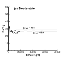
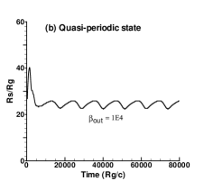
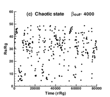
Figure 1: Time-variations of the shock location $R_{\rm s}$ at the equator for flows with $\lambda$= 1.65 and $\epsilon=6.89\times 10^{-3}$ for the case of $R_{\rm out}$ = 50$R_{\rm g}$. Depending on the parameter $\beta_{\rm out}$ of the magnetic field strength, the states of the flow are categorized into three types: (a) steady state in weak magnetic fields, (b) quasi-periodic state in intermediate magnetic fields and (c) chaotically variable state in strong magnetic fields. In (a), the shock locations for $\beta_{\rm out}$ = $10^{5}$ and $10^{9}$ are attained 28.4 and 26.8$R_{\rm g}$, respectively. In (c), the shock locations are shown by the filled circle because there exist multiple shocks or no shock during the evolution.

We check whether the flow is subject to the magnetorotational instability (MRI) and whether we are able to resolve the fastest growing MRI mode or not. The stringent diagnostics of space resolution for the MRI instability has been examined in 3D magnetized flow (Hawley et al., 2011). Therefore, its application to our 2D magnetized flow may be limited to some extent. The critical wavelength of the instability mode is given by $\lambda_{\rm c}=2\pi v_{\rm A}/\sqrt{3}\Omega$, where $v_{\rm A}$ and $\Omega$ are the Alfven velocity and the angular velocity (Balbus & Hawley, 1998; Hawley et al., 2011). A criterion value $Q_{\rm x}$ of the MRI resolution is defined by

$$Q_{\rm x}=\frac{\lambda_{\rm c}}{\Delta x},$$ (9)

where $\Delta x$ is the mesh sizes $\Delta R$ and $\Delta z$ in the radial and vertical directions, respectively. When $Q_{\rm x}\gg$ 1, the flow is unstable against the MRI instability, otherwise the flow is stable. The analyses of our flows show that $Q_{\rm R}<$ 1 and $Q_{\rm z}<$ 1 over most region of the flow except for the funnel region along the rotational axis in category (a), and $40>Q_{\rm R}>5$ and $50>Q_{\rm z}>10$ near the equatorial plane in categories (b) and (c), indicating that we are able to resolve the MRI in later categories. We also calculate the normalized Reynolds stress $\alpha_{\rm gas}=\langle\rho v_{\rm R}\delta v_{\rm\phi}\rangle/\langle p_{\rm g}\rangle$ and the normalized Maxwell stress $\alpha_{\rm mag}=\langle 2B_{\rm R}B_{\rm\phi}\rangle/\langle B^{2}\rangle$ which are space-averaged over a region near the equator and are time-averaged over a final duration time of the evolution. Here, $\alpha_{\rm gas}$ and $\alpha_{\rm mag}$ are roughly 0.06 – 0.03 and 0.06 – 0.3, respectively, for $\beta_{\rm out}$ = 4000.

Figure 2: Analytical transonic flow for the parameters of $\lambda$ = 1.35, $\epsilon=1.98\times 10^{-6}$ and $\gamma$ = 1.6 under the assumption of vertical hydrostatic equilibrium of the flow. Vertical arrow represents the location of shock transition. Overall arrows indicate the direction of flow motion towards the black hole.

Table 1: Parameters of the specific angular momentum $\lambda$, the specific energy $\epsilon$, the adiabatic index $\gamma$ and the mass accretion rate $\dot{M}$, and flow variables of the density $\rho_{\rm out}$, the radial velocity $v_{\rm out}$, the temperature $T_{\rm out}$, the relative disk thickness $(h/R)_{\rm out}$, the Keplerian angular momentum $(\lambda_{\rm K})_{\rm out}$ at the outer radial boundary $R_{\rm out}=200R_{\rm g}$ for Sgr A* and mesh sizes $\Delta R/R_{\rm g}$, $\Delta z/R_{\rm g}$ used in models A and B.

									${\rm Mesh\;sizes}$
$\lambda$	$\varepsilon$	$\gamma$	$\dot{M}$	$\rho_{\rm out}$	$v_{\rm out}$	$T_{\rm out}$	$(h/R)_{\rm out}$	$(\lambda_{\rm K})_{\rm out}$	$(0\leq\frac{R}{R_{\rm g}}\leq 2,\;\frac{|z|}{R_{\rm g}}\leq 2)$	$({\rm otherwise})$
($2GM/c$)	($c^{2}$)		($M_{\odot}\>{\rm yr}^{-1}$)	(${\rm g}\;{\rm cm}^{-3}$)	($c$)	($\rm K$)		($2GM/c$)	($R_{\rm g}$)	($R_{\rm g}$)
1.35	1.98E-6	1.6	4.0E-6	5.87E-19	-0.0498	2.55E9	0.432	10.0	0.2	0.495

3.2 Application to the Long-Term Flares of Sgr A*

3.2.1 Setup of the Flow Parameters

Here, we consider a supermassive black hole with $M=4\times 10^{6}M_{\odot}$ for Sgr A*. Based on the assumption that the Wolf-Rayet star ${\rm IRS}$ 13 $\rm E3$ is the dominant source of accreting matter onto Sgr A* and a stellar wind temperature $T_{\rm wind}$ = 0.5 or 1.0 keV, Mościbrodzka et al. (2006) estimated a net specific angular momentum $\lambda=1.68-2.16$, Bernoulli constant $\epsilon=1.98\times 10^{-6}$ – 3.97$\times 10^{-6}$ and mass accretion rate $\dot{M}$ = (2 – 4) $\times 10^{-6}M_{\odot}$ yr^-1 for the accretion flow around Sgr A*. Referring to this work and Okuda & Molteni (2012), we consider here a set of parameters $\lambda$ = 1.35, $\epsilon=1.98\times 10^{-6}$ and a mass accretion rate $\dot{M}$ = 4.0 $\times 10^{-6}M_{\odot}$ yr^-1 and examine the time-variations of the magnetized low angular momentum flow, focusing on the long-term flares of Sgr A*.

In Fig. 2, we show the analytical transonic solution corresponding to the above $\lambda$ and $\epsilon$, where flow after crossing the outer critical point ‘a’ continues to proceed along the supersonic branch ‘ab’ and enters the event horizon of the black hole (Okuda & Molteni, 2012), where the outer critical point $R_{\rm a}$ is 1.68 $\times 10^{4}R_{\rm g}$. However, the flow chooses to jump from point ‘b’ to ‘c’ at $R_{\rm s}\sim 20R_{\rm g}$ to become subsonic because the entropy generated through the shock is higher compared to that of the supersonic branch. Subsequently, the flow passes through the inner critical point and becomes supersonic again along ‘cd’ before crossing the event horizon.

Since we focus on the long-term variability of Sgr A*, it is desirable for us to set the standing shock at large radius. Taking account of the relation between the numerical shock location and the adopted outer boundary radius in subsections 2.3 and 3.1, we set the outer radial boundary at $R_{\rm out}=200R_{\rm g}$ and determine the primitive variables $\rho$, v and $p$ at the boundary from the transonic solutions. As to the parameter $\beta_{\rm out}$ of the magnitude of the magnetic field, considering of the effects of magnetic field on the standing shock in subsection 3.1, we adopt two cases of $\beta_{\rm out}$= 1000 (model A) and 5000 (model B).

Table 1 shows the model parameters of the specific angular momentum $\lambda$, the specific energy $\epsilon$, the adiabatic index $\gamma$ and the mass accretion rate $\dot{M}$, and the flow variables of the density $\rho_{\rm out}$, the radial velocity $v_{\rm out}$, the temperature $T_{\rm out}$, the relative disk thickness $(h/R)_{\rm out}$, the Keplerian angular momentum $(\lambda_{\rm K})_{\rm out}$ at the outer radial boundary $R_{\rm out}=200R_{\rm g}$ for Sgr A* and mesh sizes $\Delta R/R_{\rm g},\Delta z/R_{\rm g}$ used in models A and B. In our adiabatic flow model, the specific angular momentum $\lambda$ is kept constant everywhere. The Keplerian angular momentum $\lambda_{\rm K}\propto R^{1/2}$ and is larger than the constant $\lambda$ in most of regions considered here.

The computational domain consists of $0\leq R\leq R_{\rm out}=200R_{\rm g}$ and $-z_{\rm out}\leq z\leq z_{\rm out}$ with $z_{\rm out}=200R_{\rm g}$. The number of meshes is $(N_{\rm R},N_{\rm z})$ = (410, 820). The mesh size is $\Delta R=\Delta z=0.2R_{\rm g}$ for $0\leq R\leq 2R_{\rm g},-2R_{\rm g}\leq z\leq 2R_{\rm g}$, and otherwise $\Delta R=\Delta z=0.495R_{\rm g}$.

After the steps described in section 2, we obtain the steady state hydrodynamical flow. Fig. 3 shows the profiles of temperature $T$, Mach number of the radial velocity $v_{\rm R}$ and the relative disk thickness $h/R$ at the equator (Left) and the 2D density contours log $\rho$ in g cm^-3 (Right) for the steady hydrodynamical flow. The disk thickness is geometrically thick as $h/R\simeq 0.4$. The shock is clearly distinguished as a sharp discontinuity at $R=64.8R_{\rm g}$. In the 2D contours of the density, the shock extends from the equatorial plane obliquely toward the upper stream.

The numerically obtained shock location $R_{\rm s}=64.8R_{\rm g}$ at the equatorial plane differs considerably from the analytical value $R_{\rm s}\sim$ 20$R_{\rm g}$ as discussed in subsection 2.3. Then, using the 2D steady hydrodynamical flow as the initial conditions of the magnetized flow, we examine the time-variations of the shock location $R_{\rm s}$ and the total luminosity $L$ of the magnetized flow.

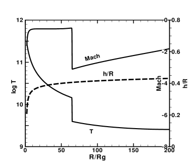
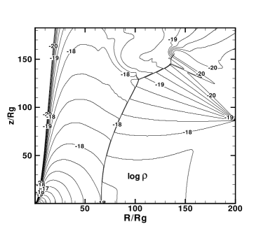
Figure 3: Profiles of temperature $T$, Mach number of the radial velocity $v_{\rm R}$ and relative disk thickness $h/R$ at the equator (Left) and 2D density contours log $\rho$ in g cm^-3 (Right) for the hydrodynamical steady state flow. The shock is clearly distinguished as a sharp discontinuity at $R=64.8R_{\rm g}$. In the contours, only the first quadrant is presented and the shock extends from the equatorial plane obliquely toward the upper stream.

The luminosity $L$ is given by

$$L=\int q_{\rm ff}{\rm d}V,$$ (10)

where $q_{\rm ff}$ is the free-free bremsstrahlung emission rate per unit volume and here only ion-electron bremsstrahlung is considered under a single temperature model and $L$ is integrated over all computational zones. If we consider a two-temperature model and a stronger magnetic field as $\beta_{\rm out}$ = 1 – 10, the synchrotron radiation dominates the free-free emission (Okuda, 2014) and equation (10) may be invalid in such synchrotron radiation dominated region. However, the adiabatic assumption of the energy equation is considered to be reasonable everywhere because even the synchrotron cooling rate is far smaller than the transfer rate of the advected thermal energy. The mass-outflow rate $\dot{M}_{\rm out}$ is defined by the total rate of outflow through the outer boundaries ($z=\pm~{}z_{\rm out}$) in the z direction,

$$\dot{M}_{\rm out}=\int_{0}^{R_{\rm out}}2\pi\rho(R,z_{\rm out})v_{\rm z}(R,z_{\rm out})RdR-\int_{0}^{R_{\rm out}}2\pi\rho(R,-z_{\rm out})v_{\rm z}(R,-z_{\rm out})RdR,$$ (11)

where $v_{\rm z}(R,z)$ is the vertical velocity as a function of the coordinate ($R$, $z$). The outflow rate $\dot{M}_{\rm R_{\rm out}}$ through the outer boundary ($R=R_{\rm out}$) in the R direction is not included in the above equation.

3.2.2 Evolution of the Magnetized Flow

In our models, the centrifugal pressure-supported shock possesses high temperature and high density post-shock matter and is termed as post-shock corona (hereafter PSC) (Aktar et al., 2015). The existence of the PSC is a good tracer of the flow evolution in our models. As is found in subsection 3.1, we expect the flow is subject to the MRI also in models A and B. Actual analyses of the models show that $100>Q_{\rm R}>$ 10 and $100>Q_{\rm z}>$ 20 at $R>6R_{\rm g}$ near the equatorial plane, indicating that we are able to resolve the MRI. Hereafter, focusing on model A, we explain the whole evolution of the magnetized flow, because the pattern of time-variability of $L$ and $R_{\rm s}$ in model B is basically similar to that in model A.

Fig. 4 shows the profiles of the density $\rho$, the angular velocity $\Omega$, the gas pressure $p$, the magnetic pressure $p_{\rm m}$, the normalized Reynolds stress $\alpha_{\rm gas}$ and the normalized Maxwell stress $\alpha_{\rm mag}$ for model A, where $\Omega$ and pressure $p$ are given in units of $c^{3}/GM$ and dyn/cm², respectively, and the variables are space-averaged between $-2R_{\rm g}\leq z\leq 2R_{\rm g}$ and are time-averaged over the last duration time $1.1\times 10^{7}-1.2\times 10^{7}$ s. In the plots of density and angular velocity, their initial values and the Keplerian angular velocity are also shown. In spite of the MRI activity during the evolution, the averaged angular velocity is rather distributed along its initial value and is far smaller than the Keplerian one. The strong jump at the shock in the initial density is smoothened out in the averaged density due to the irregularly oscillating shock. The Maxwell stress is much stronger than the Reynolds stress in the inner region and $\mid\alpha_{\rm mag}\mid$ is $\sim$ 0.1 in the region of $60R_{\rm g}\leq R\leq 170R_{\rm g}$, where the shock oscillates. The averaged magnetic pressure is far smaller than the gas pressure in the outer region due to the given large $\beta_{\rm out}$ at $R=R_{\rm out}$ but increases toward the inner region. These distributions of $\Omega$, $p$, $p_{\rm m}$, $\alpha_{\rm gas}$ and $\alpha_{\rm mag}$ are similar to those at the same radial region in the low angular momentum magnetized flows by Proga & Begelman (2003b).

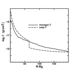
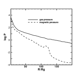
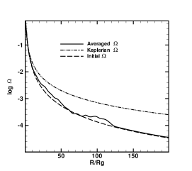
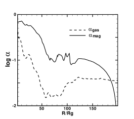
Figure 4: Radial profiles of the density $\rho$, the angular velocity $\Omega$, the gas pressure $p$, the magnetic pressure $p_{\rm m}$, the normalized Reynolds stress $\alpha_{\rm gas}$ and the normalized Maxwell stress $\alpha_{\rm mag}$ for model A. The variables are space-averaged between $-2R_{\rm g}\leq z\leq 2R_{\rm g}$ and are time-averaged over the last duration time $1.1\times 10^{7}-1.2\times 10^{7}$ s. In the plots of density and angular velocity, the initial values and the Keplerian angular velocity are also shown.

After a transient initial phase, the magnetic field is amplified rapidly by the MRI and the MHD turbulence near the equatorial plane, as well as by the advection of the magnetic field lines to the inner boundary. The flow and shock structures are considerably different from the initial hydrodynamical flow and show very asymmetric features above and below the equatorial plane due to the magnetic field. The luminosity and the shock location vary by more than a factor of 3 in models A and B. Fig. 5 shows the time sequence of the velocity vectors and 2D contours of the density $\rho$, the magnetic field strength $\mid\textbf{B}^{2}\mid$ and the ratio $\beta$ of gas to magnetic pressure at times $t=2\times 10^{5}$ (a), $4\times 10^{5}$ (b), $8\times 10^{5}$ (c), $1.2\times 10^{6}$ (d) and $1.6\times 10^{6}$ (e) s (left to right) in model A, where the velocity vectors and the magnetic field strength $\mid\textbf{B}\mid$ are shown in unit vector and in unit of Gauss (G), respectively. To compare with the observations of Sgr A*, henceforth we use time unit of seconds. The luminosity and the shock location at (a), (b), (c), (d) and (e) are $2.9\times 10^{34},3.6\times 10^{34},3.1\times 10^{34},1.6\times 10^{34}$ and $1.3\times 10^{35}$ erg s^-1 and 108, 122, 140, 187 and 128$R_{\rm g}$, where the luminosities at (d) and (e) are minimal and maximal, respectively, in the entire time-evolution of the luminosity (see Fig. 7). The final time $1.6\times 10^{6}$ s is indicated as (e) in the curves of $L$ and $R_{\rm s}$ in Fig. 7. During the times depicted, the MRI grows and stabilizes. As a result, MHD turbulence develops near the equator.

A high magnetic blob is formed in the inner region within the PSC region. Here, we designate the high magnetic blob as a spherical bubble-like shape with high magnetic field strength which is clearly found in the third and fourth panels of Fig. 5. The high magnetic blob is distinguished from the broader PSC region behind the centrifugal pressure-supported shock. The PSC region behind the shock has high density and high temperature but the magnetic field just behind the shock is not so strong as that in the high magnetic blob. The blob goes forward with increasing magnetic field strength, continues to expand diffusively and obliquely across the equator up to $R\sim 140R_{\rm g}$ at time (d) and then fades out as a filament-like feature at time (e). This morphological evolution reflects directly on the time evolution of the luminosity and the shock location in Fig. 7.

Focusing on (d) and (e) of Fig. 5 where the luminosity becomes minimal and maximal, respectively, we examined the magnitude $\mid\textbf{B}\mid$ of the magnetic field. Fig. 6 shows the contours of $\mid\textbf{B}\mid$ in the inner region for model A. We find here that 50 G $\geq\mid\textbf{B}\mid\geq$ 20 G in (d) and 30 G $\geq\mid\textbf{B}\mid\geq$ 3 G in (e) at 20$R_{\rm g}\geq R\geq 5R_{\rm g}$ on the equator, while 10 G $\geq\mid\textbf{B}\mid\geq$ 0.1 G in (d) and 1 G $\geq\mid\textbf{B}\mid\geq$ 0.1 G in (e) at 200$R_{\rm g}\geq R\geq 50R_{\rm g}$, respectively, where $\beta_{\rm out}$=1000 corresponds to the magnetic field strength $\mid\textbf{B}\mid\sim$ 0.1 G at the outer radial boundary. In each contour of Fig. 6, there exist two distorted central masses of high magnetic field $\mid\textbf{B}\mid\geq$ 60 G. They are very unstable and yield filamentous projections of the magnetic field which develop into a spherical bubble-like shape (high magnetic blob) in the outer region.

The behavior of $\beta$ in the bottom panel of Fig. 5 is compatible with the evolution of the magnetic field shown in the same figure. These panels of Fig. 5 show how the shock wave evolves due to the effect of the magnetic pressure. During the initial phases (a) – (b), due to the MRI activity, $\beta$ becomes low as $\sim 10$ in the high magnetic blob region which extends to $R$ = 50 and 70$R_{\rm g}$, respectively, in (a) and (b) but $\beta\sim$ 100 – 1000 outside the high magnetic blob.

On the other hand, $\beta$ is very small in the funnel region along the rotational axis, making these regions nearly magnetically dominated. Accordingly, the gas is strongly accelerated along the rotational axis, compared with the initial hydrodynamical model. The outflow region is roughly separated into two regions: one of a high velocity jet in the funnel region along the rotational axis and another one with a wind at the vertical outer boundaries. The jet has velocities between $0.1-0.8c$ within the funnel region and the wind has roughly the escape velocity $v_{\rm e}\sim 0.07c$ outside the funnel region. The averaged mass-outflow rate from the jet and the wind occupies 40 – 50$\%$ of the input accretion rate in models A and B and the remainder gas falls into the black hole. The mass outflow rate of the jet is comparable to that of the wind. Since the magnetic field is not axisymmetric to the equator, the flow features are different above and below the equator, but the qualitative behavior is similar in both regions. After $t\sim 2\times 10^{6}$ s, the MRI activity settles to a nearly stable state, but the luminosity and the shock location are strongly variable with irregular oscillation and large amplitude (see Fig. 7).

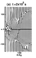
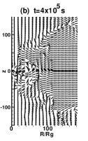
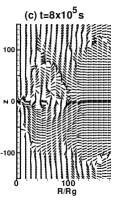
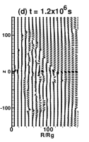
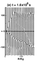
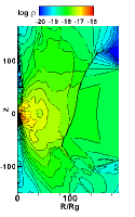
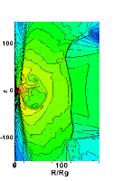
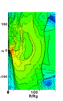
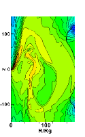
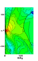
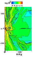
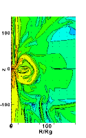
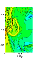
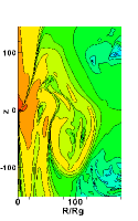
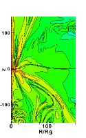
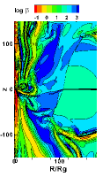
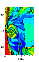
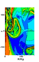
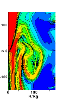
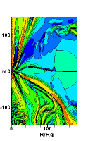
Figure 5: Time variations of unit velocity vectors and 2D contours of density $\rho$, magnetic field strength $\textbf{B}^{2}$ and ratio $\beta$ of gas pressure to magnetic pressure at times $t=2\times 10^{5}$ (a), $4\times 10^{5}$ (b), $8\times 10^{5}$ (c), $1.2\times 10^{6}$ (d) and $1.6\times 10^{6}$ (e) s (left to right) in model A. The luminosity is minimal in (d) and then becomes maximal in (e), while the shock location at equator is maximal and minimal at the former and the latter times, respectively.

3.2.3 Time Variations of the Luminosity and the Shock Location

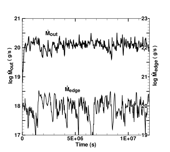
Figure 8: Time evolutions of the mass-outflow rate $\dot{M}_{\rm out}$ (g s^-1) and the mass-inflow rate $\dot{M}_{\rm edge}$ (g s^-1) at the inner edge in model A. To compare clearly the phases of their variations, different vertical scales for $\dot{M}_{\rm out}$ and $\dot{M}_{\rm edge}$ are taken here. .

We take the output data for the luminosity and the shock location at every time interval of 100 $R_{\rm g}/c$ ($\sim 4\times 10^{3}$ s). Therefore, the time resolution in our simulations is one hour at most. Fig. 7 shows the variations of the luminosity $L$ and the shock position $R_{\rm s}$ at the equatorial plane in model A with the parameter $\beta_{\rm out}=1000$ of magnetic field strength. Here, the arrow at $t=1.6\times 10^{6}$ s on the abscissa denotes the epoch (e) during the time evolution of the flow described in Fig 5. The shock and the luminosity oscillate irregularly with time scales of $\sim 10^{5}-10^{6}$ s, and the average $L$ is $\sim 4.0\times 10^{34}$ erg s^-1. It should be noticeable that the gap of $R_{\rm s}$ curve at the phase $t\sim 6.5\times 10^{6}$ shows a possibility of the moving away of the shock from the outer boundary. Fig. 8 shows the time variations of the mass-outflow rate $\dot{M}_{\rm out}$ and the mass-inflow rate $\dot{M}_{\rm edge}$ at the inner edge in model A. Here, in order to compare more clearly the phases of their variations, we take different vertical scales for $\dot{M}_{\rm out}$ and $\dot{M}_{\rm edge}$. $L$, $R_{\rm s}$, $\dot{M}_{\rm out}$ and $\dot{M}_{\rm edge}$ in model A show irregular, but recurrent variations roughly in a time-scale of $\sim 5\times 10^{5}$ s. These irregular oscillations remain constant without fading. From the time variations of $L$, $R_{\rm s}$, $\dot{M}_{\rm out}$ and $\dot{M}_{\rm edge}$, we find strong correlations between $L$ and $\dot{M}_{\rm edge}$ and between $R_{\rm s}$ and $\dot{M}_{\rm out}$ and an anti-correlation between $L$ and $R_{\rm s}$.

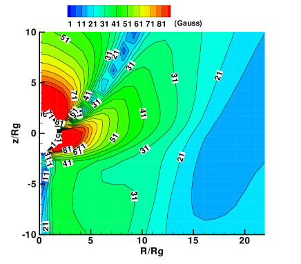
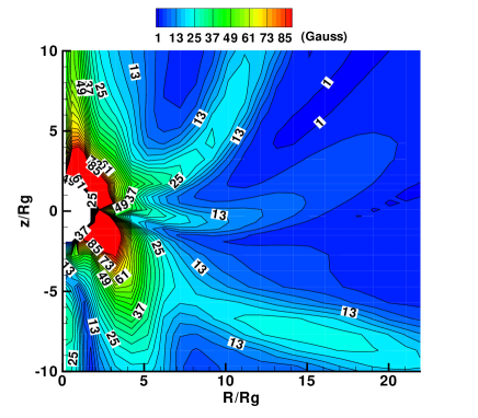
Figure 6: 2D contours of the strength $\mid\textbf{B}\mid$ (Gauss) of the magnetic field in the inner region at $t=1.2\times 10^{6}$ s (left) and $1.6\times 10^{6}$ s (right) for model A. Two distorted central masses of high magnetic field in each contour are very unstable and yield filamentous projections of the magnetic field which develop into spherical bubble-like shape in the outer region.

The overall evolution of the flow is similar to the initial one during $t\leq 2\times 10^{6}$ s described in sub-subsection 3.2.2. The shock location $R_{\rm s}$ at the equator is initially at $R_{\rm s}\sim 65R_{\rm g}$. The shock and the high magnetic blob within the PSC begin to expand with increasing magnetic pressure and the shock reaches a maximal location $R_{\rm s}\sim$ 187$R_{\rm g}$ at $t=1.2\times 10^{6}$ s (phase (d) of Fig. 5) and then recedes back, while the expanding high magnetic blob is diffused out. When the shock is expanding through the outermost region, a new high density blob with high temperature appears in the inner region and another inner shock is formed in front of the expanding high density blob, due to the interaction of the blob with the accreting matter. During the successive evolution, the outer and inner shocks show complex behavior and these processes are repeated irregularly. When the outer shock expands to its maximal position, the mass-outflow rate is maximal and the luminosity attains its minimal value. Conversely, when the shock shrinks to its minimal position, the luminosity attains the maximal values, while the mass-outflow rate is minimal. This behavior is similar to the relation between the luminosity and the pulsating radius in variable stars as well known (Christy, 1966). We find also that most of the luminosity is emitted from the PSC region and the contribution from the outside of the PSC region is less than 10 percent of the total luminosity. After the MRI activity settles to a stable state, the shock finally moves back and forth between $R_{\rm s}$= 60 – 170$R_{\rm g}$ with an irregular time interval of $\sim 5\times 10^{5}$ s. Due to the variable shock location, the luminosity varies by more than a factor of 3. Fig. 9 shows the time variations of $L$ and $R_{\rm s}$ for model B with the parameter $\beta_{\rm out}=5000$ of magnetic field strength. The shock and the luminosity oscillate irregularly with time scales of $\sim 10^{5}-10^{6}$ s and the average $L$ is $\sim 3.0\times 10^{34}$ erg s^-1, i.e. the same as model A. The maximum shock locations in model B are a little smaller than those in model A, because of its smaller magnetic field strength.

Fig. 10 shows the power density spectra of luminosity $L$ for models A (Left) and B (Right). Though we can not find very clear peaks of the power density spectra in both models, model A shows a break frequency at $2.0\times 10^{-6}$ Hz together with another weak signal at $\sim 1.1\times 10^{-5}$ Hz. On the other hand, model B denotes peak frequencies at $2.5\times 10^{-6}$ and $1.1\times 10^{-5}$ Hz, including two more additional weak features at $5.4\times 10^{-6}$ and $3.0\times 10^{-5}$ Hz. These frequencies may be harmonics of the original oscillation with $2.5\times 10^{-6}$ Hz. As a result, we observe a peak signal at frequency (2.0 – 2.5) $\times 10^{-6}$ Hz along with a common weak signature at $1.1\times 10^{-5}$ Hz in both models, which correspond to periods (4.6 – 5.8) ($\sim$ 5) days and 25 hrs, respectively. The larger period $\sim 5$ days corresponds to the time-scale of the irregular shock oscillation between 60$R_{\rm g}\leq R\leq 170R_{\rm g}$. Fig. 11 shows the Mach number of the radial velocity on the equator at times $t=4.6\times 10^{6}$ (solid line), $5.7\times 10^{6}$ (dash-dot line) and 6.2 $\times 10^{6}$ (dashed line) s in model A. Here, there exist another shock phenomena behind the outer shock for each curve. The shock corresponds to the inner shock mentioned in sub-subsection 3.2.3. The inner shocks are weak compared with the outer shock and the shock features are complicated. From the animation of Mach number versus radius, we recognize that the inner shock oscillates irregularly and rapidly. The inner shocks also contribute to the luminosity because the density and the temperature behind the inner shock are higher than those behind the outer shock, although the Mach number is smaller than that in the outer shock. However, the variability pattern of the inner shock is not clear as the one found in the outer shock oscillation and may be recognized as a weak signature at $\nu$ = 1.1$\times 10^{-5}$ Hz in the power density spectrum. We conclude that the time-variability with two different periods in models A and B is due to an oscillating outer strong shock with another more rapid oscillation of the inner weak shock.

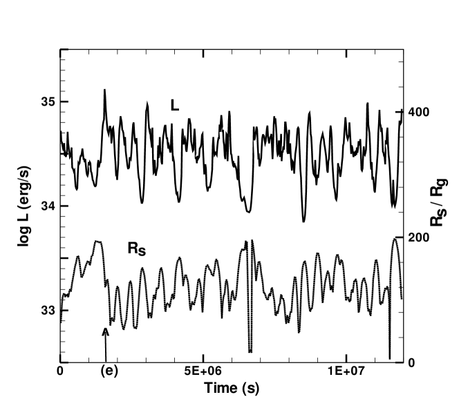
Figure 7: Time evolutions of luminosity $L$ (erg s^-1) and shock position $R_{\rm s}$ (in $R_{\rm g}$ units) at the equatorial plane in the magnetized model A with the parameter $\beta_{\rm out}=1000$ of magnetic field strength. When the shock expands to a maximal position, the luminosity attains its minimal value. Conversely, when the shock shrinks to its minimal position, the luminosity is maximal. The arrow at $t=1.6\times 10^{6}$ s on the abscissa denotes the epoch (e) during the time evolution of the flow described in Fig 5.

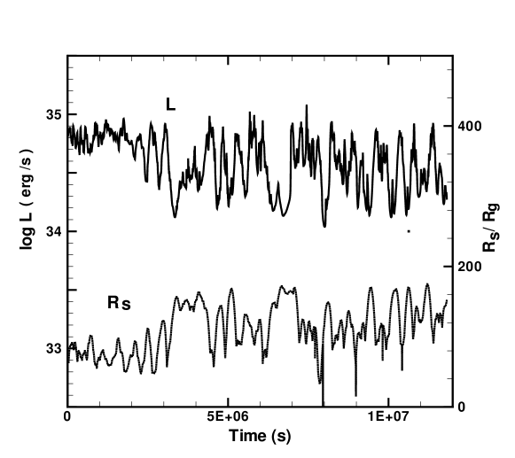
Figure 9: Same as Fig 7 but for model B with the parameter $\beta_{\rm out}$ = 5000 of magnetic field strength.

Figure 10: Power density spectra of luminosity $L$ for models A (left) and B (right). A break frequency at $2.0\times 10^{-6}$ Hz with another weak signal at $\sim 1.1\times 10^{-5}$ Hz in model A and peak frequencies at $2.5\times 10^{-6}$ and $1.1\times 10^{-5}$ Hz in model B are observed.

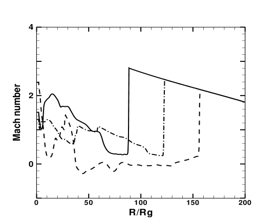
Figure 11: Radial profiles of Mach number of the radial velocity -$v_{\rm R}$ on the equator at $t=4.6\times 10^{6}$ (solid line), $5.7\times 10^{6}$ (dash-dot line) and $6.2\times 10^{6}$ (dashed line) s in model A. The outer strong shock oscillates at 60 $\leq R\leq$ 170 and the inner weak shock oscillates irregularly and rapidly far below the outer shock.

Our magnetized flow are compared with the same as reported by Proga & Begelman (2003b). They started with the initial conditions of the Bondi spherical accretion flow, but with a constant angular momentum $\lambda$ in the region of $-h_{\rm out}\leq z\leq h_{\rm out}$ at the outer boundary and used values of $\lambda$ = 1 – 2 similar to ours, but Bernoulli constant $\epsilon=0$, instead of our positive value as $\epsilon=1.98\times 10^{-6}$. The 1.5D transonic solutions for these parameters of $\epsilon$ and $\lambda$ never yield the standing shock formation under the vertical hydrostatic equilibrium assumption. They examined the magnetized flow over a wide range up to the Bondi radius and with $\beta_{\rm out}$ = $10^{5}$ – $10^{7}$. Their results of the global MRI effects on the angular velocity, the magnetic pressure and the Maxwell stress and of the time variation of the accretion rate are similar to those in our models. But the quasi-periodic oscillation (QPO)-like features of the accretion rate are not found in their results. Because the QPO-like variabilities of the luminosity and the mass outflow rate in our models are due to the shock wave oscillation driven by the magnetic field.

3.2.4 Relevance to Sgr A*

The supermassive black hole candidate Sgr A* shows quiescent and flare states. The rapid flares over hours to day of Sgr A* have been detected in multiple wavebands from radio, sub-millimetre and IR to X-ray. Recent Chandra, Swift and XMM-Newton observations over long durations show that flares with X-ray luminosity $L_{\rm x}>10^{34}$ erg s^-1 occur at a rate of $\sim 1$ per day, while luminous flares with $L_{\rm x}>10^{35}$ erg s^-1 occur every 5 – 10 days (Degenaar et al. 2013; Neilsen et al. 2013, 2015; Ponti et al. 2015). The results of the time dependent simulations in this work may be compared with these long-term flares of Sgr A*. In the present magnetized models A and B, the luminosities vary as $8\times 10^{33}$ – $1.4\times 10^{35}$ erg s^-1. The averaged maximal luminosity due to the outer shock is $\sim 1.0\times 10^{35}$ erg s^-1 and the variable maximal luminosity due to the inner shock is roughly estimated to be $\sim 2.5\times 10^{34}$ erg s^-1.

However, it should be noticed that the above luminosities might be underestimated when the synchrotron radiation dominates the free-free emission as mentioned in sub-subsection 3.2.1. Yuan et al. (2003) proposed reasonable models of the quiescent and rapid flare states in X-ray spectra, considering synchrotron and Inverse Compton emissions by accelerated electrons, where the X-ray radiation emitted at the flare state is two orders of magnitude larger than that at the quiescent state. They showed the quiescent model with a strong magnetic field of $\mid\textbf{B}\mid\sim$ 20 G at $R\leq 10R_{\rm g}$ and the X-ray flare model with a weak magnetic field $\mid\textbf{B}\mid\leq$ 1 G in the emitting region. From the best fit parameters of the mean spectrum of very bright flares, Ponti et al. (2017) showed that large magnetic field amplitude ($\mid\textbf{B}\mid\sim$ 30 G) is observed at the start of the X-ray flare and then drops to $\mid\textbf{B}\mid\sim 4.8$ G at the peak of the X-ray flare. This scenario to the rapid flares may be adaptable also to the long-term flares of Sgr A*. In this respect, it is useful for us to refer the time evolution of the magnetic field strength in Fig 5. The luminosity is minimal as $\sim 1.6\times 10^{34}$ erg s^-1 at $t=1.2\times 10^{6}$ s (d) and then attains the maximal of $\sim 1.1\times 10^{35}$ erg s^-1 at $1.6\times 10^{6}$ s (e). This time sequence is regarded as the evolution of the quiescent state to flare state. The analyses of the magnetic field evolution show that $\mid\textbf{B}\mid\geq$ 30 G in (d) and $\mid\textbf{B}\mid\geq$ 7 G in (e) at $R\leq 10R_{\rm g}$ on the equator as mentioned in sub-subsection 3.2.2. That is, the features of the magnetic field strength at the inner region of the flow in (d) and (e) qualitatively represent well those at the quiescent and X-ray flare states, respectively, shown by Yuan et al. (2003) and Ponti et al. (2017). This suggests strongly that actual maximal luminosity in our models may increases considerably through the synchrotron radiation in the inner region and we expect the maximal luminosity due to the outer shock exceeds far $\sim 10^{35}$ erg s^-1. On the other hand, an upper limit on the quiescent luminosity of Sgr A* above 10 keV was recently derived to be $L_{\rm X_{\rm q,10-79keV}}$ $\leq 2.9\times 10^{34}$ erg s^-1 (Zhang et al., 2017). If we regard the minimal luminosity $\sim 10^{34}$ erg s^-1 in our models as the quiescent luminosity, the luminosity variation of $L>10^{34}$ erg s^-1 occurring at a rate of 25 hrs and $L>10^{35}$ erg s^-1 occurring approximately every 5 days in this work is qualitatively compatible with the observed long-term flares of Sgr A*.

4 Summary and Discussion

We examined the effects of magnetic field on low angular momentum flows with standing shock around the black hole and, adopting fiducial parameters of a specific energy $\epsilon$ = $1.96\times 10^{-6}$, a specific angular momentum $\lambda=1.35$, and magnetic parameters $\beta_{\rm out}$= 1000 (model A) and 5000 (model B), applied the magnetized flow models to the long-term flares of Sgr A*. The results of our 2D simulations are summarized below.

(1) After the MRI is activated, MHD turbulence develops near the equator. The magnetic field adds more pressure in the system which is enhanced by compression behind the shock and thus breaks the original equilibrium of the standing shock of the HD configuration. As a result, the centrifugally supported shock moves back and forth between 60 $R_{\rm g}\leq R\leq 170R_{\rm g}$. In addition to the outer shock, another inner weak shock appears irregularly with rapid variations due to the interaction of the expanding high magnetic blob with the accreting matter below the outer shock.

(2) This process repeats irregularly with an approximate time-scale of (4 – 5) $\times 10^{5}$ s ($\sim$ 5 days) with an accompanying smaller amplitude modulation with a period of $\sim 0.9\times 10^{5}$ s (25 hrs). The time-variability with two different periods is attributed to the oscillating outer strong shock together with the rapidly oscillating inner weak shock. Due to the variable shock location, the luminosities vary by more than a factor of $3$ and the average values are 3 – 4 $\times 10^{34}$ erg s^-1.

(3) The variability patterns of the order of $\sim$ 5 days and 25 hrs found in models A and B are compatible with the latest results of long-term flares of Sgr A* with X-ray luminosity $L_{\rm x}>10^{34}$ erg s^-1 occurring at a rate of $\sim 1$ per day and with luminous flares with $L_{\rm x}>10^{35}$ erg s^-1 occurring approximately every 5 – 10 days by Chandra, Swift and XMM-Newton monitoring of Sgr A*.

The time-scale of the irregular variability in the present model depends on the location of the centrifugally supported shocks in the accretion flow. The irregular variabilities in these models are due to the competition among the gravity, centrifugal force and pressure gradient forces at the shock, that is, the unstable behavior of the standing shock. It is known that a standing shock in adiabatic accretion flow is unstable against axisymmetric perturbations under some conditions and that the dynamical time-scale of the instability is of the order of $\sim R_{\rm s}/v_{\rm-}$, where $v_{\rm-}$ is the pre-shock velocity (Nakayama, 1994). Therefore, the smaller the shock position $R_{\rm s}$ the faster the shock variability is. If we had started with initial conditions in the magnetized flow leading to a smaller shock location, a more rapid variability could be obtained, and vice versa. Accordingly, the inclusion of other physical processes like viscosity (Das et al., 2014), the magnetic resistivity, or other radiative cooling mechanisms (Chakrabarti et al., 2004), like synchrotron radiation in a stronger magnetic field and different configurations of the magnetic field may change the present findings.

The observed rapid flares of Sgr A* with time-scales of hours to day show time lags of flares between multi-wavelength bands, such as the 20 – 40 minutes lag between 22 GHz and 43 GHz and about two hours lag between X-ray and submilimeter in Sgr A* (Yusef-Zadeh et al. 2008, 2009). At present, the time lags of the long-term flares, for example, between the X-ray and radio wavelengths have not been observed yet because simultaneous long time series at such wavelengths are limited. However, it is natural for us to consider there exist the time lag phenomena of the long-term flares. Such time lags may be caused by different physical processes or in different regions of the accretion inflow-outflow system. In this connection, we may need an additional picture to describe the flare events of Sgr A*. Here, we regard the average emission obtained in the models as the nearly constant emission of the quiescent state. On the other hand, the variable emission in Sgr A* may be probably caused by the intermittent outflows, as found by the present results. We can speculate that magnetized clumps from the shocked material near $z\sim 200R_{\rm g}$ are swept by the high speed jet. We then argue that the impact between the clumps could produce a radio flare with a time lag of $200R_{\rm g}/c\sim$ 2 hrs. The radio emission could be observed as synchrotron radiation in the surrounding of the clumps if electrons are relativistically accelerated by the enhanced magnetic field via Fermi shock or magnetic reconnection acceleration (de Gouveia Dal Pino & Lazarian, 2005; de Gouveia Dal Pino & Kowal, 2015; Kadowaki et al., 2015; Singh et al., 2015).

The present low angular momentum flow model is too simple to reproduce the detailed observed spectra of Sgr A*. With the inclusion of the physical processes described above and a longer term MHD simulation in a larger computational domain will allow us to track the full evolution of this system and the different regimes of the variability phenomena in low angular momentum flows.

We would like to thank an anonymous referee for many useful comments. C.B.S. acknowledges support from the Brazilian agency FAPESP (grant 2013/09065-8) and was also supported by the I-Core center of excellence of the CHE-ISF. This work has made use of the computing facilities of the Laboratory of Astroinformatics (IAG/USP, NAT/Unicsul), whose purchase was made possible by FAPESP (grant 2009/54006-4). AN thanks GD, SAG; DD, PDMSA and Director, URSC for encouragement and continuous support to carry out this research. EMDGP acknowledges partial support from the Brazilian agencies FAPESP (2013/10559-5) and CNPq (306598/2009-4) grants.

References

- Aktar et al. (2015) Aktar R., Das S., & Nandi A. 2015, MNRAS, 453, 3414
- Balbus & Hawley (1991) Balbus S. A., & Hawley J. F. 1991, ApJ, 376, 214
- Balbus & Hawley (1998) Balbus S. A., & Hawley J. F. 1998, Rev.Mod. Phys., 70,1
- Ball et al. (2016) Ball D., Özel F., Psaltis D., & Chan C.-K. 2016, ApJ, 826,77
- Becker et al. (2011) Becker P. A., Das S., & Le T. 2011, ApJ, 743, 47
- Bondi (1952) Bondi H. 1952, MNRAS, 112, 195
- Chakrabarti (1989) Chakrabarti S. K. 1989, ApJ, 347, 365
- Chakrabarti & Molteni (1993) Chakrabarti S. K., & Molteni D. 1993, ApJ, 417, 671
- Chakrabarti (1996) Chakrabarti S. K. 1996, ApJ, 464, 664
- Chakrabarti et al. (2004) Chakrabarti S. K., Acharyya K., & Molteni D. 2004, A & A, 421, 1
- Chan et al. (2009) Chan C-K., Liu S., Fryer C. L., Psaltis D., Özel, F., Rockefeller, G., & Melia, F. 2009, ApJ., 701, 521
- Christy (1966) Christy R. F. 1966, ApJ., 144, 108
- Czerny & Mościbrodzka (2008) Czerny B., & Mościbrodzka M. 2008, J. Phys. Conf. Ser.,131, 012001
- Das et al. (2009) Das S., & Becker P. A., Le T. 2009, ApJ, 702, 649
- Das et al. (2014) Das S., Chattopadhyay I., Nandi A., & Molteni D. 2014, MNRAS, 442, 251
- Degenaar et al. (2013) Degenaar N., Miller J. M., Kennea J., Gehrels N., Reynolds M. T., & Wijnands R. 2013, ApJ, 769, 155
- de Gouveia Dal Pino & Lazarian (2005) de Gouveia Dal Pino E. M., & Lazarian A. 2005, A & A, 441, 845
- de Gouveia Dal Pino & Kowal (2015) de Gouveia Dal Pino E. M., & Kowal G. 2015, ASSL, 407, 373
- Dexter et al. (2009) Dexter J., Agol E., & Fragile P. C. 2009, ApJ., 703, L142
- Dodds-Eden et al. (2010) Dodds-Eden K., Sharma P., Quataert E., Genzel R., Gillessen, S., Eisenhauer, F., & Porquet, D. 2010, ApJ., 725, 450
- Eckart et al. (2006) Eckart A., Schödel R., Meyer L., Trippe S., Ott T., & Genzel R. 2006, A&A, 455, 1
- Fukue (1986) Fukue J. 1986, PASJ, 38, 167
- Genzel et al. (2010) Genzel R., Eisenhauer F., & Gillessen S. 2010, Rev. Mod. Phys., 82, 3121
- Genzel et al. (2003) Genzel R., Schödel R., Ott T., Eckart A., Alexander T., Lacombe F., Rouan D., & Aschenbach B. 2003, Nature, 425, 934
- Ghez et al. (2004) Ghez A. M. et al. 2004, ApJ., 601, L159
- Hawley & Balbus (1991) Hawley J. F., & Balbus S. A. 1991, ApJ, 376, 223
- Hawley et al. (2011) Hawley J. F., Guan X., & Krolik J. H. 2011, ApJ, 738, 84
- Igumenshchev & Abramowicz (1999) Igumenshchev I. V., & Abramowicz M. A. 1999, MNRAS, 303, 309
- Igumenshchev & Abramowicz (2000) Igumenshchev I. V., & Abramowicz M. A. 2000, ApJS, 130, 463
- Igumenshchev et al. (2003) Igumenshchev I. V., Narayan R., & Abramowicz M. A. 2003, ApJ, 592, 1042
- Kadowaki et al. (2015) Kadowaki L. H. S., de Gouveia Dal Pino, E. M., & Singh C. B. 2015, ApJ, 802, 113
- Li et al. (2013) Li J., Ostriker J., & Sunyaev R. 2013, ApJ., 767, 105
- Li, Yuan & Wang (2017) Li Y.-P., Yuan F., & Wang Q. D. 2017, MNRAS, 468, 2552
- Machida et al. (2000) Machida M., Hayashi M. R., & Matsumoto R. 2000, ApJ, 532, L67
- Machida et al. (2001) Machida M., Matsumoto R., & Mineshige S. 2001, PASJ, 53, L1
- Meyer et al. (2006a) Meyer L., Schödel R., Eckart A., Karas V., Dovčiak M., & Duschl W.J. 2006a, A&A, 458, L25
- Meyer et al. (2006b) Meyer L., Eckart A., Schödel R., Duschl W.J., Mužić K., Dovčiak M., & Karas, V. 2006b, A&A, 460, 15
- Mignone et al. (2007) Mignone A., Bodo G., Massaglia S., Matsakos T., Tesileanu O., Zanni C., & Ferrari A. 2007, ApJS, 170, 228
- Molteni et al. (1996) Molteni D., Ryu D., & Chakrabarti S. K. 1996, ApJ., 470, 460
- Mościbrodzka et al. (2006) Mościbrodzka M., Das T.K., & Czerny B. 2006, MNRAS, 370, 219
- Nakayama (1994) Nakayama K., 1994, MNRAS, 270, 871
- Narayan et al. (2003) Narayan R., Igumenshchev I. V., & Abramowicz, M. A. 2003, PASJ, 55, L69
- Narayan & McClintock (2008) Narayan R., & McClintock J.E. 2008, New Astron. Rev., 51, 733
- Narayan et al. (2012) Narayan R., Sädowski A., Penna, R. F., & Kulkarni, A. K. 2012, MNRAS, 426, 3241
- Narayan & Yi (1994) Narayan R., & Yi I. 1994, ApJ, 428, L13
- Narayan & Yi (1995) Narayan R., & Yi I. 1995, ApJ, 452, 710
- Neilsen et al. (2013) Neilsen J. et al. 2013, ApJ, 774, 42
- Neilsen et al. (2015) Neilsen J. et al. 2015, ApJ, 799, 199
- Okuda (2014) Okuda T. 2014, MNRAS, 441, 2354
- Okuda & Molteni (2012) Okuda T., & Molteni D. 2012, MNRAS, 425, 2413
- Okuda & Das (2015) Okuda T., & Das S. 2015, MNRAS, 453, 147
- Paczyńsky & Wiita (1980) Paczyńsky B., Wiita, P. J. 1980, A&A, 88, 23
- Ponti et al. (2015) Ponti G. et al. 2015, MNRAS, 454, 1525
- Ponti et al. (2017) Ponti G. et al. 2017, MNRAS, 468, 2447
- Proga & Begelman (2003a) Proga D., & Begelman M. C. 2003a, ApJ, 582, 69
- Proga & Begelman (2003b) Proga D., & Begelman M. C. 2003b, ApJ, 592, 767
- Ressler et al. (2017) Ressler S. M., Tchekhovskoy A., Quataert E., & Gammie C. F. 2017, MNRAS, 467, 3604
- Roberts et al. (2017) Roberts S. R., Jiang Y.-F., Wang Q. D., & Ostriker J. P. 2017, MNRAS, 466, 1477
- Sarkar & Das (2016) Sarkar B., & Das S. 2016, MNRAS, 461, 190
- Shakura & Sunyaev (1973) Shakura N.I., & Sunyaev R.A. 1973, A&A, 24, 337
- Singh et al. (2015) Singh C. B., de Gouveia Dal Pino, E. M., & Kadowaki L. H. S. 2015, ApJ, 799, L20
- Stone & Pringle (2001) Stone J. M., & Pringle J. E. 2001, MNRAS, 322, 461
- Stone et al. (1999) Stone J. M., Pringle J. E., & Begelman M. C. 1999, MNRAS, 310, 1002
- Trippe et al. (2007) Trippe S., Paumard T., Ott T., Gillessen S., Eisenhauer F., Martins F., & Genzel, R. 2007, MNRAS, 375, 764
- Yuan (2011) Yuan F. 2011, in Morris M.R., Wang Q.D., Yuan F., eds, ASP Conf. Ser. 439, The Galactic Center: A Window to the Nuclear Environment of Disk Galaxies. Astron. Soc. Pac., San Francisco, p. 346
- Yuan et al. (2012) Yuan F., Bu D., & Wu M. 2012, ApJ, 761, 130
- Yuan et al. (2015) Yuan F., Gan, Z., Narayan, R., Sadowski, A., Bu, D., & Bai, X. 2015, ApJ, 804,101
- Yuan et al. (2009) Yuan F., Lin, J., Wu, K., & Ho, L. C. 2009, MNRAS, 395, 2183
- Yuan & Narayan (2014) Yuan F., & Narayan R. 2014, ARA&A, 52, 529
- Yuan et al. (2003) Yuan F., Quataert E., & Narayan R. 2003, ApJ, 598, 301
- Yuan et al. (2004) Yuan F., Quataert E., & Narayan R. 2004, ApJ, 606, 894
- Yuan et al. (2012) Yuan F., Wu M., & Bu D. 2012, ApJ, 761, 129
- Yusef-Zadeh et al. (2006) Yusef-Zadeh F. et al. 2006, ApJ, 644, 198
- Yusef-Zadeh et al. (2008) Yusef-Zadeh F. et al. 2008, ApJ, 682, 361
- Yusef-Zadeh et al. (2009) Yusef-Zadeh F. et al. 2009, ApJ, 706, 348
- Yusef-Zadeh et al. (2011) Yusef-Zadeh F., Wardle M., Miller-Jones J.C.A., Roberts D.A., Grosso N., & Porquet D. 2011, ApJ, 729, 44
- Zhang et al. (2017) Zhang S. et al. 2017, ApJ, 843, 96