MOCZ for Blind Short-Packet Communication: Some Practical Aspects

Abstract

We will investigate practical aspects for a recently introduced blind (noncoherent) communication scheme, called modulation on conjugate-reciprocal zeros (MOCZ), which enables reliable transmission of sporadic and short-packets at ultra-low latency in unknown wireless multipath channels, which are static over the receive duration of one packet. Here the information is modulated on the zeros of the transmitted discrete-time baseband signal’s $z-$transform. Due to ubiquitous impairments between transmitter and receiver clocks a carrier frequency offset (CFO) will occur after a down-conversion to the baseband, which results in a common rotation of the zeros. To identify fractional rotations of the base angle in the zero-pattern, we propose an oversampled direct zero testing decoder to identify the most likely one. Integer rotations correspond to cyclic shifts of the binary message, which we compensate by a cyclically permutable code (CPC). Additionally, the embedding of CPCs into cyclic codes, allows to exploit additive error correction which reduces the bit-error-rate tremendously. Furthermore, we use the trident structure in the signals autocorrelation to estimate timing offsets and the channels effective delay spread. We finally demonstrate how these impairment estimations can be largely improved by receive antenna diversity, which enables extreme bursty reliable communication at low latency and SNR.

I Introduction

We introduced in [1, 2] a novel blind (noncoherent) communication scheme for the physical layer, called modulation on conjugate-reciprocal zeros (MOCZ), to reliably transmit sporadic short-packets of fixed size over unknown wireless multipath channels with bandwidth $W$ at an incredible low-latency. Here the information of the packet is modulated on the zeros of the transmitted discrete-time baseband signal’s $z-$transform. We will call the discrete-time baseband signal a MOCZ symbol, similar to an orthogonal frequency division multiplexing (OFDM) symbol, which is a finite length sequence of complex-valued coefficients. These coefficients will then modulate a continuous-time pulse shape at a sample period of $T=1/W$ to generate the continuous-time baseband waveform. Since the MOCZ symbols (sequences) are neither orthogonal in time nor frequency domain, the MOCZ design can be seen as a non-orthogonal multiplexing scheme. After up-converting to the desired carrier frequency, the transmitted passband signal will propagate in space such that, due to reflections, diffractions, and scattering, different delays of the attenuated signal will interfere at the receiver. Hence, multipath propagation causes a time-dispersion which results in a frequency-selective fading channel [3]. Due to ubiquitous impairments between transmitter and receiver clocks a carrier frequency offset (CFO) will be present after a down conversion to the baseband. Doppler shifts due to relative velocity causes additional frequency dispersion which can be also approximated in first order by a CFO. This is a known weakness in many multi-carrier modulation schemes, such as OFDM [3, 4, 5, 6], and various approaches have been developed to estimate or eliminate the CFO effect. A common approach for OFDM systems is to learn the CFO in a training phase or from blind estimation algorithms, such as MUSIC [7] or ESPRIT [8]. Furthermore, due to the unknown distance and asynchronous transmission, a timing offset (TO) of the received symbol has to be determined as well, which will otherwise destroy the orthogonality of the OFDM symbols [9, 5.1],[10]. By “sandwiching” the data symbol between two training symbols a timing and frequency offset can be estimated [11],[12]. By using antenna arrays at the receiver, antenna diversity of a single-input-multiple output (SIMO) system can be exploited to improve the performance [5].

Whereas OFDM is typically used in long frames, consisting of many successive OFDM symbols and hence much longer signal lengths, we consider here only one single symbol transmission with a very short signal length. This places high demands on such a bursty signaling scheme, since timing and carrier frequency offsets have to be addressed from only one received symbol. Here our MOCZ scheme will be a promising solution. Since any communication will be scheduled and timed on the MAC layer by a certain bus, running with a known bus clock-rate, timing-offsets of the symbols can be assumed as fractions of the bus clock-rate. We will introduce here an improved receiver design for a coded binary MOCZ (BMOCZ) scheme and demonstrate by bit-error-rate (BER) simulations the robustness against these impairments.

In the MOCZ design, a CFO will result in an unknown common rotation of all received zeros. Since the angular zero spacing in a BMOCZ symbol of length $K+1$ is given by a base angle of $2\pi/K$, a fractional rotation can be easily obtained at the receiver by an oversampling during the post-processing to identify the most likely transmitted zeros (zero-pattern). Rotations, which are integer multiples of the base angle, correspond to cyclic shifts of the binary message word. By using a cyclically permutable code (CPC) for the binary message, the BMOCZ symbol becomes invariant against any cyclic shift and hence against any CFO. This prevents any further symbol transmissions for estimating the CFO, which will reduce overhead, latency, and complexity. As a byproduct, this has the appealing feature of providing a CFO estimation from the decoding process of a single BMOCZ symbol. Furthermore, due to the embedding into a cyclic code, such as BCH codes, we can use their error correction capabilities to improve the BER and moreover the block error-rate (BLER) performance tremendously. By measuring the energy of the expected symbol length with a sliding window in the received signal, we can identify arbitrary TOs at the receiver. We will show the robustness of the TO estimation analytically, which reveals another strong property of the MOCZ design.

At last, we will combine CFO and TO with error correction over multiple receive antennas and demonstrate antenna diversity of the SIMO system. By simulating BER over the received SNR for various average power delay profiles, with constant and exponential decay as well as random sparsity constraints, we will demonstrate the performance in various indoor and outdoor scenarios by using the simulation framework Quadriga [13].

I-A Notation

We will use small letters for complex numbers in ${\mathbb{C}}$. Capital Latin letters denote natural numbers ${\mathbb{N}}$ and refer to fixed dimensions, where small letters are used as indices. Boldface small letters denote row vectors and capitalized letters refer to matrices. Upright capital letters denote complex-valued polynomials in ${\mathbb{C}}[z]$. We will denote the first $N$ natural numbers in ${\mathbb{N}}$ as $[N]:=\{0,1,\dots,N-1\}$. For $K\in{\mathbb{N}}$ we denote by $K+[N]=\{K,K+1,\dots K+N-1\}$ the $K-$shift of the set $[N]$. The Kronecker-delta symbol is given by $\delta_{nm}$ and is $1$ if $n=m$ and $0$ else. For a complex number $x=a+jb$, given by its real part $\operatorname{Re}(x)=a\in{\mathbb{R}}$ and imaginary part $\operatorname{Im}(x)=b\in{\mathbb{R}}$ with imaginary unit $j=\sqrt{-1}$, its complex-conjugation is given by ${\overline{x}}=a-jb$ and its absolute value by $|x|=\sqrt{x{\overline{x}}}$. For a vector ${\mathbf{x}}\in{\mathbb{C}}^{N}$ we denote by ${\overline{{\mathbf{x}}^{-}}}$ its complex-conjugated time-reversal or conjugate-reciprocal, given as ${\overline{x_{k}^{-}}}={\overline{x_{N-k}}}$ for $k\in[N]$. We use ${\mathbf{A}}^{*}={\overline{{\mathbf{A}}}}^{T}$ for the complex-conjugated transpose of the matrix ${\mathbf{A}}$. For the $N\times N$ identity matrix we write ${\mathbf{I}}_{N}$ and for a $N\times M$ matrix with all elements zero we write ${\mathbf{O}}_{N,M}$. By ${\mathbf{D}}_{{\mathbf{x}}}$ we refer to the diagonal matrix generated by ${\mathbf{x}}\in{\mathbb{C}}^{N}$. The $N\times N$ unitary Fourier matrix ${\mathbf{F}}={\mathbf{F}}_{N}$ is given entry-wise by $f_{l,k}=e^{-j2\pi lk/N}/\sqrt{N}$ for $l,k\in[N]$. By $\mathbf{T}\in{\mathbb{R}}^{N\times M}$ denote the elementary Toeplitz matrix given element-wise as $\delta_{n-1m}$. The all one and all zero vectors in dimension $N$ will be denoted by ${\mathbf{1}}_{N}$ and ${\mathbf{0}}_{N}$, respectively. The $\ell_{p}$-norm of a vector ${\mathbf{x}}=(x_{0},\dots,x_{N-1})\in{\mathbb{C}}^{N}$ is given by $\left\|{\mathbf{x}}\right\|_{p}=(\sum_{k=0}^{N-1}|x_{k}|^{p})^{1/p}$ for $p\geq 1$. If $p=\infty$ we write $\left\|{\mathbf{x}}\right\|_{\infty}=\max_{k}|x_{k}|$ and for $p=2$ we set $\left\|{\mathbf{x}}\right\|_{2}=\left\|{\mathbf{x}}\right\|$. The expectation of a random variable $x$ is denoted by ${\mathbb{E}[x]}$.

II System Model and Requirements

We are interested in a blind and asynchronous transmission of a short single MOCZ symbol at a designated bandwidth $W$. In this “one-shot” communication we assume no synchronization and no packet scheduling between transmitter and receiver. Such extreme sporadic, asynchronous, and ultra short-packet transmissions are required, for example, in critical control applications, exchange of channel state information (CSI), signaling protocols, secret keys, authentication, commands in wireless industry applications, or initiation, synchronization and channel probing packets to prepare for longer or future transmission phases. By choosing the carrier frequency, transmit sequence length, and bandwidth accordingly, a receive duration in the order of the channel delay spread can be obtained, which pushes the latency at the receiver to the lowest possible. Since the next generation of mobile wireless networks aims for large bandwidths with carrier frequencies beyond $10$Ghz, in the so called mmWave band, the transmitted signal duration will be in the order of nano seconds. Hence, even at moderate mobility, the wireless channel in an indoor or outdoor scenario can be considered as approximately time-invariant over such a short time duration. On the other hand, wideband channels are highly frequency selective, which is due to the superposition of different delayed versions (echos) of the transmitted signal at the receiver. This makes equalizing in time-domain very challenging and is commonly simplified by using OFDM instead. But conventional OFDM requires an additional cyclic prefix to convert the frequency-selective channel to parallel scalar channels and in coherent mode it requires additional pilots (training) to learn the channel coefficients. This will increase the latency for short messages dramatically.

For a communication in mmWave band massive antenna arrays are exploited to overcome the large attenuation, which increases the complexity and energy consumption in estimating the huge amount of channel parameters and becomes the bottleneck in mmWave MIMO systems, especially for mobile scenarios. However, in a sporadic communication only one symbol will be transmitted and a next symbol may follow at an unknown time later. In a random access channel (RACH), a different user may transmit the next symbol from a different location, which will therefore experience an independent channel realization. Hence, the receiver can barely use any channel information learned from past communications. OFDM systems approach this by transmitting many successive OFDM symbols as a long frame, to estimate the channel impairments, which will cause a considerable overhead and latency if only a few data-bits need to be communicated. Furthermore, to achieve orthogonal subcarriers in OFDM, the cyclic prefix has to be at least as long as the channel impulse response (CIR) length, resulting in signal lengths at least twice as the CIR length during which the channel also needs to be static. Using OFDM signal lengths much longer than the coherence time might be not feasible for fast time-varying block-fading channels. Furthermore, the maximal CIR length needs to be known at the transmitter and if underestimated will lead to a serious performance loss. This is in high contrast to our MOCZ design, where the signal length can be chosen for a single MOCZ symbol independently from the CIR length. The goal in this work is to address the ubiquitous impairments of the MOCZ design under such ad-hoc communication assumptions and signal lengths in the order of the CIR length.

After up-converting the MOCZ symbol, which is a discrete-time complex-valued baseband signal ${\mathbf{x}}=(x_{0},x_{1},\dots,x_{K})\in{\mathbb{C}}^{K+1}$ of two-sided bandwidth $W$, to the desired carrier frequency $f_{c}$, the transmitted passband signal will propagate in space. Regardless of directional or omnidirectional antennas, the signal will be reflected and diffracted at point-scatters, resulting in different delays of the attenuated signal which interfere at the receiver if the maximal delay spread $T_{d}$ of the channel is larger than the sample period $T=1/W$. Hence, the multipath propagation causes time dispersion resulting in a frequency-selective fading channel. Due to ubiquitous impairments between transmitter and receiver clocks an unknown frequency offset $\Delta f$ will be present after the down-conversion to the received continuous-time baseband signal

$$\tilde{r}(t)=r(t)e^{j2\pi t\Delta f}.$$ (1)

By sampling $\tilde{r}_{n}=\tilde{r}(nT)$ at the sample period $T$, the received discrete-time baseband signal can be represented by a tapped delay line (TDL) model. Here the channel action is given as the convolution of the MOCZ symbol ${\mathbf{x}}$ with a finite impulse response $\{h_{\ell}\}$, where the $\ell$th complex-valued channel tap $h_{\ell}$ describes the $\ell$th averaged path over the bin $[\ell T,(\ell+1)T)$, which we model by a circularly symmetric Gaussian random variable in $\mathcal{CN}(0,s_{\ell}p^{\ell})$ for $l\in[L]$ and zero elsewhere. The average power delay profile (PDP) of the channel can be sparse and exponentially decaying, where $s_{\ell}\in\{0,1\}$ defines the sparsity pattern of $S=|{\operatorname{supp}({\mathbf{h}})}|=\sum_{\ell=0}^{L-1}s_{\ell}=\left\|{\mathbf{s}}\right\|_{1}$ non-zero coefficients and $p\leq 1$ the exponential decay rate. To obtain equal average transmit and average receive power we will eliminate in our analysis the overall channel gain by normalizing the CIR realization ${\mathbf{h}}=(h_{0},\dots,h_{L-1})$ by its average energy $\sum_{l=0}^{L-1}s_{l}p^{l}$ (for a given sparsity pattern), such that ${\mathbb{E}[\left\|{\mathbf{h}}\right\|^{2}]}=1$. The convolution output is then additively distorted by Gaussian noise $w_{n}\in\mathcal{CN}(0,N_{0})$ of zero mean and variance (average power density) $N_{0}$ for $n\in{\mathbb{N}}$ as

$$\begin{split}\tilde{r}_{n}&=e^{jn\phi}\sum_{k=0}^{K}x_{k}h_{n-\tau_{0}-k}\!+\!e^{jn\phi}w_{n}=\sum_{k=0}^{K}e^{jk\phi}x_{k}e^{j(n-k)\phi}h_{n-\tau_{0}-k}\!+\!\tilde{w}_{n}=\sum_{k=0}^{K}\tilde{x}_{k}\tilde{h}_{n-\tau_{0}-k}\!+\!\tilde{w}_{n}.\end{split}$$ (2)

Here $\phi=2\pi\Delta f/W\mod 2\pi\in[0,2\pi)$ denotes the carrier frequency offset (CFO) and $\tau_{0}\in{\mathbb{N}}$ the timing offset (TO), which marks the delay of the first symbol coefficient $x_{0}$ via the first channel path $h_{0}$, measured in integer multiples of the sample time $T$. The modulated MOCZ symbol $\tilde{\mathbf{x}}\in{\mathbb{C}}^{K}$ will have rotated coefficients $\tilde{x}_{k}=e^{jk\phi}x_{k}$ as well as the channel $\tilde{h}_{\ell}=e^{j(\ell+\tau_{0})\phi}h_{\ell}$, which will be also effected by a global phase $\tau_{0}\phi$. Since the channel taps have a uniform independent phase the distribution does not change. By the same argument, the Gaussian noise distribution is not alternated by the phase, hence we have $\tilde{w}_{n}\in\mathcal{CN}(0,N_{0})$ for any $n$ and $\phi$.

In [2, 1] a good signal-codebook is given for Binary MOCZ (BMOCZ) for the set of normalized Huffman sequences $\mathscr{C}(R,K)=\left\{\left.{\mathbf{x}}\in{\mathbb{C}}^{K+1}\rule[-2.5pt]{0.0pt}{10.0pt}\;\right|\;{\mathbf{a}}(R,K)={\mathbf{x}}*{\overline{{\mathbf{x}}^{-}}},x_{0}>0\right\}$, i.e., by all ${\mathbf{x}}\in{\mathbb{C}}^{K+1}$ with positive first coefficientand “impulsive-like“ autocorrelation [14], given by

$${\mathbf{a}}={\mathbf{a}}(R,K)={\mathbf{x}}*{\overline{{\mathbf{x}}^{-}}}=(-\eta,{\mathbf{0}}_{K},1,{\mathbf{0}}_{K},-\eta)\quad\text{with}\quad\eta=1/(R^{K}+R^{-K})$$ (3)

for some $R>1$. The absolute value of (3) forms a trident with one main peak at the center, given by the energy $\left\|{\mathbf{x}}\right\|^{2}=1$, and two equal side-peaks of $\eta\in[0,1/2)$, see Figure (1). From an analytical and empirical investigation [1], the BMOCZ symbols are most robust against noise if

$$R=R(K)=\sqrt{1+\sin(\pi/K)}>1\quad,\quad K\geq 2.$$ (4)

Hence, the BMOCZ codebook (constellation set) $\mathscr{C}=\mathscr{C}(K)$ is only determined by the number $K$. Each BMOCZ symbol (constellation, Huffman sequence) defines the coefficients of a polynomial of degree $K$, where the $K$ zeros are uniformly placed on a circle of radius $R$ or $R^{-1}$, selected by the message bits $\mathbf{m}=(m_{1},\dots,m_{K})\in\{0,1\}^{K}$ as

$${\mathrm{X}}(z)=\sum_{k=0}^{K}x_{k}z^{k}=x_{K}\prod_{k=1}^{K}(z-R^{2m_{k}-1}e^{j2\pi(k-1)/K})=x_{K}\prod_{k=1}^{K}(z-\alpha_{k}^{(m_{k})})$$ (5)

see also Figure (3). Hence, the BMOCZ encoder is defined iteratively for $q=2,\dots,K$ by its zero codeword $\boldsymbol{\alpha}(\mathbf{m})=(\alpha_{1}^{(m_{1})},\dots,\alpha_{K}^{(m_{K})})\in\mathscr{Z}\subset{\mathbb{C}}^{K}$ as

$${\mathbf{x}}_{q}=(0,{\mathbf{x}}_{q-1})-(R^{2m_{q}-1}e^{j\frac{2\pi q}{K}}{\mathbf{x}}_{q-1})\quad\text{with}\quad{\mathbf{x}}_{1}=(-R^{2m_{1}-1}e^{j\frac{2\pi}{K}},1),$$ (6)

where we normalize after the last iteration step ${\mathbf{x}}={\mathbf{x}}_{K}/\left\|{\mathbf{x}}_{K}\right\|$. From the received $N=L+K$ noisy signal samples (no CFO and TO)

$$y_{n}=\sum_{k=0}^{K}x_{k}h_{n-k}+w_{n}=({\mathbf{x}}*{\mathbf{h}})_{n}+w_{n},$$ (7)

the decoder is given as a Direct Zero Testing (DiZeT) of the received polynomial ${\mathrm{Y}}(z)=\sum_{n=0}^{N-1}y_{n}z^{n}$ at the $2K$ possible zero positions as

$$\hat{m}_{k}=\begin{cases}1,&|{\mathrm{Y}}(Re^{j2\pi\frac{k-1}{K}})|<R^{N-1}|{\mathrm{Y}}(R^{-1}e^{j2\pi\frac{k-1}{K}})|\\ 0,&\text{else}\end{cases}\quad,\quad k=1,\dots,K,$$ (8)

see [1, 2]. A global phase in ${\mathrm{Y}}(z)$ will have no affect to the DiZeT decoder and to the received zeros. But the CFO $\phi$ modulates the BMOCZ symbol in (2) and causes a rotation of its zeros by $-\phi$ in (5), which will destroy the hypothesis test of the DiZeT decoder. Hence, one needs to either estimate $\phi$ or use an outer code for BMOCZ to be invariant against an arbitrary rotation of the entire zero codebook $\mathscr{Z}$, which we will introduce in Section (IV). However, before we can apply the DiZeT decoder, we have to identify the timing offset of the symbol which yields to the convolution output in (7).

III Timing Offset and Effective Delay Spread for BMOCZ

In an asynchronous communication, the receiver does not know when a packet from a transmitter (user) will arrive. Hence, at first the receiver has to detect a transmitted packet, which is already one bit of information. We will assume that the receiver decide correctly, that in an observation window of $N_{\text{obs}}=N_{\text{noise}}+K+L$ received samples, one single MOCZ packet of length $K$ with maximal channel length of $L$ is captured. By assuming a maximal length $L$ and a known or a maximal $K$ at the receiver, the observation window can be chosen, for example, as $N_{\text{obs}}=2N$. From the noise floor knowledge at the receiver, a simple energy detector with a hard threshold over the observation window can be used for a packet detection. Then, an unknown TO $\tau_{0}\in[N_{\text{noise}}]$ and CFO $\phi\in[0,2\pi)$ will be present in the observation window

$$\tilde{r}_{n}=e^{jn\phi}({\mathbf{x}}*{\mathbf{h}})_{n-\tau_{0}}+\tilde{w}_{n}=(\tilde{\mathbf{x}}*\tilde{\mathbf{h}}\mathbf{T}^{\tau_{0}})_{n}+\tilde{w}_{n}\quad,\quad n\in[N_{\text{obs}}].$$ (9)

The challenge here is to identify $\tau_{0}$ and the efficient channel length which contains most of the energy of the instantaneous CIR realization ${\mathbf{h}}$. The estimation of these Timing-of-Arrival (TOA) parameters are usually done by observing the same channel under many symbol transmission, to obtain a sufficient statistic of the channels PDP [15], [16]. Since we only have one observation available, a good estimation is very challenging.

The efficient (instantaneous) channel length $L_{\text{eff}}$, defined by an energy concentration window, will be much less than the maximal channel length $L$, due to blockage and attenuation by the environment, which might also cause a sparse, clustered, and exponential decaying power delay profile. For the MOCZ scheme, it is essential to correctly identify in the window (9) the first received sample $h_{0}x_{0}$ from the transmitted symbol ${\mathbf{x}}$, or at least do not miss it, since it will carry most of the energy if $h_{0}$ is the line of sight (LOS) path. It was shown in [2] that for the optimal radius in BMOCZ, $x_{0}$ carries in average $1/4$ to $1/5$ of the BMOCZ symbol energy, see also Figure (1). On the other hand, an overestimated channel length $L_{\text{eff}}$ will reduce the overall bit-error performance because the receiver collects unnecessary noise samples.

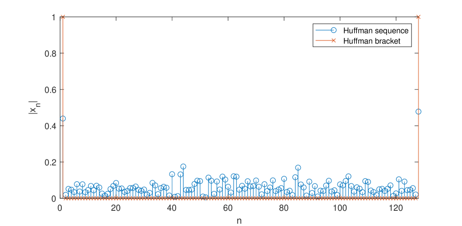
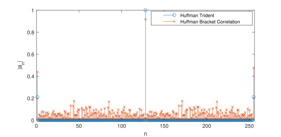
Figure 1: Left figure shows the magnitudes of a Huffman sequence for $K=127$ in blue and the absolute Huffman bracket in red. The right figure shows the autocorrelation magnitudes as well as the correlation between bracket and Huffman sequence, which both reveal a trident.

Since we assume no CSI at the receiver, the channel characteristic, i.e., the instantaneous power delay profile, has to be determined entirely from the received MOCZ symbol. We will introduce here an efficient approach for the BMOCZ design, by exploiting the radar properties of the Huffman sequences, to obtain excellent estimation of the timing offset and the effective channel delay in moderate and high SNR.

Huffman sequences have an impulsive autocorrelation (3), originally designed for radar applications, and are therefore very suitable to measure the channel impulse response [17]. Since the transmitted Huffman sequence is still unknown at the receiver, we can not correlate the received signal with the correct Huffman sequence to retrieve the CIR. Instead, we will use an approximative universal Huffman sequence, which is just the first and last peak of a typical Huffman sequence, expressed by the impulses $(\boldsymbol{\delta}_{0})_{k}=\delta_{0k}$ and $(\boldsymbol{\delta}_{K})_{n}=\delta_{Kk}$ for $k\in[K+1]$ as

$$\boldsymbol{\varkappa}_{\psi}=\boldsymbol{\delta}_{0}+e^{j\psi}\boldsymbol{\delta}_{K}\in{\mathbb{C}}^{K+1}$$ (10)

which we call the $K-$Huffman bracket of phase $\psi$. Since the first and last coefficients are

$$x_{0}=\sqrt{R^{2\left\|\mathbf{m}\right\|_{1}-K}\eta}\quad,\quad x_{K}=-\sqrt{R^{-2\left\|\mathbf{m}\right\|_{1}+K}\eta}$$ (11)

see [2], typical Huffman sequences, i.e., having same amount of ones and zeros, will have

$$|x_{0}|^{2}=|x_{K}|^{2}=\eta.$$ (12)

By correlating the modulated Huffman sequence $\tilde{\mathbf{x}}$ with the Huffman bracket $\boldsymbol{\varkappa}_{\psi}$ we keep the locational properties of the Huffman autocorrelation (trident)

$$\breve{{\mathbf{a}}}={\overline{\boldsymbol{\varkappa}_{\psi}^{-}}}*\tilde{\mathbf{x}}=(e^{-j\psi}x_{0},e^{-j\psi}\dot{\tilde{\mathbf{x}}},x_{0}+e^{j(K\phi-\psi)}x_{K},\dot{\tilde{\mathbf{x}}},e^{jK\phi}x_{K})\quad,\quad\tilde{\mathbf{x}}=\mathring{\tilde{\mathbf{x}}}+\dot{\tilde{\mathbf{x}}},$$ (13)

where $\mathring{{\mathbf{x}}}=x_{0}\boldsymbol{\delta}_{0}+x_{K}\boldsymbol{\delta}_{K}$ denotes the exterior signature and $\dot{{\mathbf{x}}}=(0,x_{1},\dots,x_{K-1},0)$ the interior signature of the Huffman sequence ${\mathbf{x}}$, see Figure (1). Here, the interior signature can be seen as the data noise floor distorting the trident ${\mathbf{a}}$ in (3). Taking the absolute-squares in (13), we get for the three peaks of the approximated trident

$$|\breve{a}_{0}|^{2}=|x_{0}|^{2},|\breve{a}_{K}|^{2}=|x_{0}|^{2}+|x_{K}|^{2}-2|x_{0}x_{K}|\cos(K\phi-\psi),|\breve{a}_{2K}|^{2}=|x_{K}|^{2},$$ (14)

where the side-peaks have energy

$$E_{\text{sides}}=|x_{0}|^{2}+|x_{K}|^{2}=(R^{2\left\|\mathbf{m}\right\|_{1}-K}+R^{-2\left\|\mathbf{m}\right\|_{1}+K})\eta\leq\left\|{\mathbf{x}}\right\|^{2}=1.$$ (15)

Since $\epsilon=2\left\|\mathbf{m}\right\|_{1}-K\in[-K,K]$ we get by (3) and $2\leq R^{\epsilon}+R^{-\epsilon}\leq R^{K}+R^{-K}$ that $2\eta\leq E_{\text{sides}}\leq 1$, where the lower bound is achieved for typical sequences with $\epsilon=0$ (having the same amount of ones and zeros) and the upper bound for $\epsilon=\pm K$ (all ones or all zeros). If $\eta=1/2$ then the two coefficients (the exterior signature $\mathring{{\mathbf{x}}}$) will carry all the energy of the Huffman sequence. But then also $R=1$ and the only Huffman sequences (real valued first and last coefficient) are given by $x_{0}=\pm 1/\sqrt{2},x_{K}=\pm 1/\sqrt{2}$ and $x_{k}=0$ for $k$ else, which are the coefficients of polynomials with $K$ uniform zeros on the unit circle, see [18]. For $R$ given by (4) the autocorrelation side-lobe $\eta$ is exponentially decaying in $K$ but is bounded to $\eta\geq 1/5$ for $K=1,2,\dots,512$. Hence, $E_{\text{sides}}\geq 0.4$, such that almost half of the Huffman sequence energy is always carried in the two peaks. If the CFO would be known, we can set $\psi=K\phi-\pi$ and get for the center peak in (14)

$$E_{\text{center}}=|x_{0}|^{2}+|x_{K}|^{2}+2|x_{0}||x_{K}|\geq 4\eta\geq 0.8,$$ (16)

i.e., the energy of the center peak is roughly twice as large as the energy of the side-peaks, and reveals the trident in the approximated Huffman autocorrelation $\breve{{\mathbf{a}}}$. But , since we do not know the CFO and $K\phi-\psi\approx 2n\pi$ for some $n\in{\mathbb{N}}$ then we get $x_{0}+x_{K}\approx 0$ for typical Huffman sequences, such that the power of the center peak will vanish. Hence, in the presence of an unknown CFO the center peak does not always identify the trident. We will therefore correlate the positive Huffman bracket $\boldsymbol{\varkappa}_{0}$ with the absolute-square value of ${\mathbf{x}}$ or in presence of noise and channel with the absolute-square of the received signal $\tilde{\mathbf{r}}$, which will result approximately in

$${\mathbf{d}}={\overline{\boldsymbol{\varkappa}_{0}^{-}}}*|\tilde{\mathbf{r}}|^{2}={\overline{\boldsymbol{\varkappa}_{0}^{-}}}*|\tilde{\mathbf{x}}*\tilde{\mathbf{h}}\mathbf{T}^{\tau_{0}}|^{2}+{\overline{\boldsymbol{\varkappa}^{-}_{0}}}*|\tilde{\mathbf{w}}|^{2}\approx|\breve{{\mathbf{a}}}|^{2}*|\tilde{\mathbf{h}}\mathbf{T}^{\tau_{0}}|^{2}+|\tilde{\tilde{\mathbf{w}}}|^{2}\in{\mathbb{R}}_{+}^{N_{\text{obs}}+K}$$ (17)

where $\tilde{\mathbf{w}}$ and $\tilde{\tilde{\mathbf{w}}}$ are colored noise and

$$|\breve{{\mathbf{a}}}|^{2}=(|x_{0}|^{2},|\dot{\breve{{\mathbf{x}}}}|^{2},E_{\text{sides}},|\dot{\breve{{\mathbf{x}}}}^{-}|^{2},|x_{K}|^{2})$$ (18)

denotes the noisy trident which collects three times the instant power delay profile $|{\mathbf{h}}|^{2}$ of the shifted CIR. These three echos of the CIR will be separated if we have $K\geq L$. The approximation in (17) can be justified by the isometry property of the Huffman convolution. Briefly, $L<K$, the generated (banded) $L\times N$ Toeplitz matrix $\mathbf{T}_{{\mathbf{x}}}=\sum_{k=0}^{K}x_{k}\mathbf{T}^{k}$, for any Huffman sequence ${\mathbf{x}}\in\mathscr{C}(K)$, is a stable linear time-invariant (LTI) system, since the energy of the output satisfy for any CIR realization ${\mathbf{h}}\in{\mathbb{C}}^{L}$

$$\left\|{\mathbf{x}}*{\mathbf{h}}\right\|^{2}=\left\|{\mathbf{h}}\mathbf{T}_{{\mathbf{x}}}\right\|^{2}=\operatorname{tr}({\mathbf{h}}\mathbf{T}_{{\mathbf{x}}}\mathbf{T}_{{\mathbf{x}}}^{*}{\mathbf{h}}^{*})=\operatorname{tr}({\mathbf{h}}^{*}{\mathbf{A}}_{{\mathbf{x}}}{\mathbf{h}})=\left\|{\mathbf{x}}\right\|^{2}\operatorname{tr}({\mathbf{h}}^{*}{\mathbf{h}})=\left\|{\mathbf{x}}\right\|^{2}\left\|{\mathbf{h}}\right\|^{2}.$$ (19)

Here, ${\mathbf{A}}_{{\mathbf{x}}}=\mathbf{T}_{{\mathbf{x}}}\mathbf{T}_{{\mathbf{x}}}^{*}$ is the $L\times L$ autocorrelation matrix of ${\mathbf{x}}$, which is the identity scaled by $\left\|{\mathbf{x}}\right\|^{2}$ if $L<K$. Hence, each normalized Huffman sequence, generates an isometric operator $\mathbf{T}_{{\mathbf{x}}}$ having the best stability among all discrete-time LTI systems, as studied in [19].

III-A Timing Offset Estimation

The delay of the strongest path $|h_{s}|=\left\|{\mathbf{h}}\right\|_{\infty}$ can be identified from the maximum in (17)

$$\hat{t}=\left(\operatorname*{argmax}_{t\in[N_{\text{obs}}+K]}d_{t}\right)-K=\left(\operatorname*{argmax}_{t\in[N_{\text{obs}}-K]+K}d_{t}\right)-K,$$ (20)

where the last equality follows from the fact that both peaks in $\boldsymbol{\varkappa}_{0}$ are contributing between $K$ and $N_{\text{obs}}$. If the CIR has a LOS path, then $s=0$ and we immediately have found an estimate for the timing-offset by ${\hat{\tau}}_{0}=\hat{t}$. In case of NLOS or if the first paths are equally strong, we have to go further back and identify the first significant peak above the noise floor, since the convolution sum of the CIR with the interior signature might produce a significant peak. Let us note here, that this might result in a misidentification of the tridents center peak by (20), for example if $|h_{s}|/|h_{0}|\gg 1$. Therefore we will use as a peak threshold

$$\rho=\rho(K,{\mathbf{d}})=\frac{1}{K+1}\sum_{n=\hat{s}+\hat{\tau}_{0}}^{\hat{s}+\hat{\tau}_{0}+K}d_{n},$$ (21)

which is the average power of the Huffman sequence distorted by the channel and noise. By comparing to the noise power $N_{0}$ we found empirically to set the noise-dependent threshold to

$$\rho_{0}=\max\{\rho(K,{\mathbf{d}})/10,\dots,\rho(K,{\mathbf{d}})/100,10\cdot N_{0}\}$$ (22)

to ensure with high probability to be above the instantaneous noise energy. By using an iterative back stepping in Algorithm (1), we will stop if the sample power falls below the threshold $\rho_{0}$, which finally yields an estimate $\hat{\tau}_{0}$ of the timing-offset. In line $3$ of Algorithm (1) we update the timing-offset estimate, if the sample power is larger than the threshold and the average power of the preceding samples is larger than the threshold divided by $1+(\log b)/3$, which will be weighted by the amount $b$ of back-steps.

III-B Efficient Channel Length Estimation

Since the BMOCZ design does not need any channel knowledge at the receiver, it is also well suited for estimating the channel itself at the receiver. Here, a good channel length estimation is essential for the performance of the decoder, if the power delay profile (PDP) is decaying. At some extent, the channel delays will fade out exponentially and the receiver can cut-off the received signal by using a certain energy ratio threshold. Let us recall the average received SNR

$${\text{rSNR}}=\frac{{\mathbb{E}[\left\|{\mathbf{x}}*{\mathbf{h}}\right\|^{2}]}}{{\mathbb{E}[\left\|{\mathbf{w}}\right\|^{2}]}}=E\frac{{\mathbb{E}[\left\|{\mathbf{h}}\right\|^{2}]}}{N\cdot N_{0}}=\frac{1}{N_{0}}$$ (23)

where $E=\left\|{\mathbf{x}}\right\|^{2}=N$ is the energy of the BMOCZ symbols, which is constant for the codebook. If the power delay profile is flat, then the collected energy will be uniform and the SNR will not change if we cut the channel length at the receiver. However, the additional channel zeros will increase the confusion for the DiZeT decoder and reduce the BER performance. Therefore, the performance will decrease for increasing $L$ at a fixed symbol length $K$, see simulations in [2]. For the most interesting scenario of $K\approx L$ the BER performance loss is only $3$dB over $E_{b}/N_{0}$, but will increase dramatically if $L\gg K$. The reason for this behaviour is the collection of many noise taps, which will lead to more distortion of the transmitted zeros. Since in most realistic scenarios the PDP will be decaying, most of the channel energy will be concentrated in the first channel taps. Hence, if we cut the received signal length to $N_{\text{eff}}=K+L_{\text{eff}}$, we will reduce the channel length to $L_{\text{eff}}<L$ and improve the rSNR for non-flat PDPs with $p<1$, since it holds

$$\frac{1}{N_{0}}=\frac{N\Big{(}\sum_{l=0}^{L_{\text{eff}}-1}p^{l}+p^{L_{\text{eff}}}\sum_{l=0}^{L-L_{\text{eff}}}p^{l}\Big{)}}{N\cdot N_{0}}\approx\frac{N\sum_{l}^{L_{\text{eff}}-1}p^{l}}{(K+L)N_{0}}<\frac{N\sum_{l}^{L_{\text{eff}}-1}p^{l}}{(K+L_{\text{eff}})N_{0}}=\frac{N{\mathbb{E}[\left\|{\mathbf{h}}_{\text{eff}}\right\|^{2}]}}{N_{\text{eff}}N_{0}}.$$ (24)

Since $1/{\mathbb{E}[\left\|{\mathbf{h}}_{\text{eff}}\right\|^{2}]}\ll N/N_{\text{eff}}$ we obtain a significant gain in SNR if $L\gg K$ and $p<1$. Hence, by cutting the received signal to the effective channel length, given by a certain energy concentration, we can improve the SNR and reduce at the same time the amount of channel zeros, which we will demonstrate by simulations in Section (V-C).

Assuming the knowledge of the noise floor $N_{0}$ at the receiver, a cut-off time can be defined as the window time which, for example, contains $95\%$ of the received energy. The estimation of the efficient channel length $L_{\text{eff}}$ can be done after the detection of the timing-offset $\tau_{0}$ with Algorithm (1). We assume here that the maximal channel delay is $L$. Since the BMOCZ symbol length is $K+1$, we know that the samples ${\mathbf{r}}_{h}=(r_{\tau_{0}+K+1},\dots,r_{\tau_{0}+K+L})$ of the received time-discrete signal in (2), which is the CIR correlated by shifts of ${\mathbf{x}}$ and distorted by additive noise (we ignore here the CFO distortion since it will be not relevant for the PDP estimation), see Figure (2(a))-(2(b)). We therefore need to determine $L_{\text{eff}}$ by an energy concentration threshold, which depends on the instantaneous SNR of ${\mathbf{r}}_{h}$. We know, that the last channel tap $h_{L_{\text{eff}}}$ will be multiplied by $|x_{K}|^{2}$, which is as strong as $|x_{0}|^{2}$ in average. There are many signal processing methods to detect the efficient energy window $N_{\text{eff}}$ in the received samples, like total variation smoothing [20], or regularized least-square methods [20, 21] which promotes short window sizes (sparsity). We propose in Algorithm (2) an iterative increasing of $L_{\text{eff}}$ starting at $1$ and increase until enough channel energy is collected. Here we set the estimate channel/signal energy to

$$E_{r}=\left\|{\mathbf{r}}_{h}\right\|^{2}-LN_{0}$$ (25)

where we start with the maximal CIR length $L$. By assuming a path exponent of $p$ we can calculate a threshold for the effective energy $E_{\text{eff}}\simeq\mu E_{r}$ with $\mu=p^{LN_{0}/2E_{r}}$. The algorithm then collects as many samples $L_{\text{eff}}$ of ${\mathbf{r}}_{h}$ until the energy $E_{\text{eff}}$ is achieved and sets $N_{\text{eff}}={K}+L_{\text{eff}}$. The extracted modulated signal is then given by

$$\tilde{\mathbf{y}}=(\tilde{r}_{\hat{\tau}_{0}},\tilde{r}_{\hat{\tau}_{0}+1}\dots,\tilde{r}_{\tau_{0}+N_{\text{eff}}}),$$ (26)

which will processed further for a CFO detection and final decoding.

Algorithm 1 center-peak-back-step (CPBS)

1:$|{\mathbf{r}}|^{2}$, $\rho_{0}$, $K$, and $\hat{t}$

2:for $b=1$ to $\lfloor K/2\rfloor$ do

3:     if $|r_{\hat{t}-b}|^{2}>\rho_{0}$ $\&$ $\sum_{n=1}^{b}|r_{\hat{t}-n}|^{2}>\frac{b\rho_{0}}{1+\frac{\log b}{3}}$ then

4:         $\hat{\tau}_{0}=\hat{t}-b$

5:     end if

6:end for

7:return $\hat{\tau}_{0}$

Algorithm 2 CIR energy-detection (CIRED)

1:$|{\mathbf{r}}|^{2}$, $\hat{\tau}_{0}$, $N_{0}$, $K$, $L$, and $p$

2:$E_{r}=\sum_{\ell=1}^{L}|r_{\hat{\tau}_{0}+K+1+\ell}|^{2}-LN_{0}$;

3:$E_{\text{eff}}=|r_{\hat{\tau}_{0}+K+1}|^{2}$; $L_{\text{eff}}=1$; $\mu=p^{LN_{0}/2E_{r}}$;

4:while $E_{\text{eff}}<\mu\cdot E_{r}$  do

5:     $L_{\text{eff}}=L_{\text{eff}}+1$;

6:     $E_{\text{eff}}=E_{\text{eff}}+|r_{\hat{\tau}_{0}+K+L_{\text{eff}}}|^{2}$;

7:end while

8:return $L_{\text{eff}}$

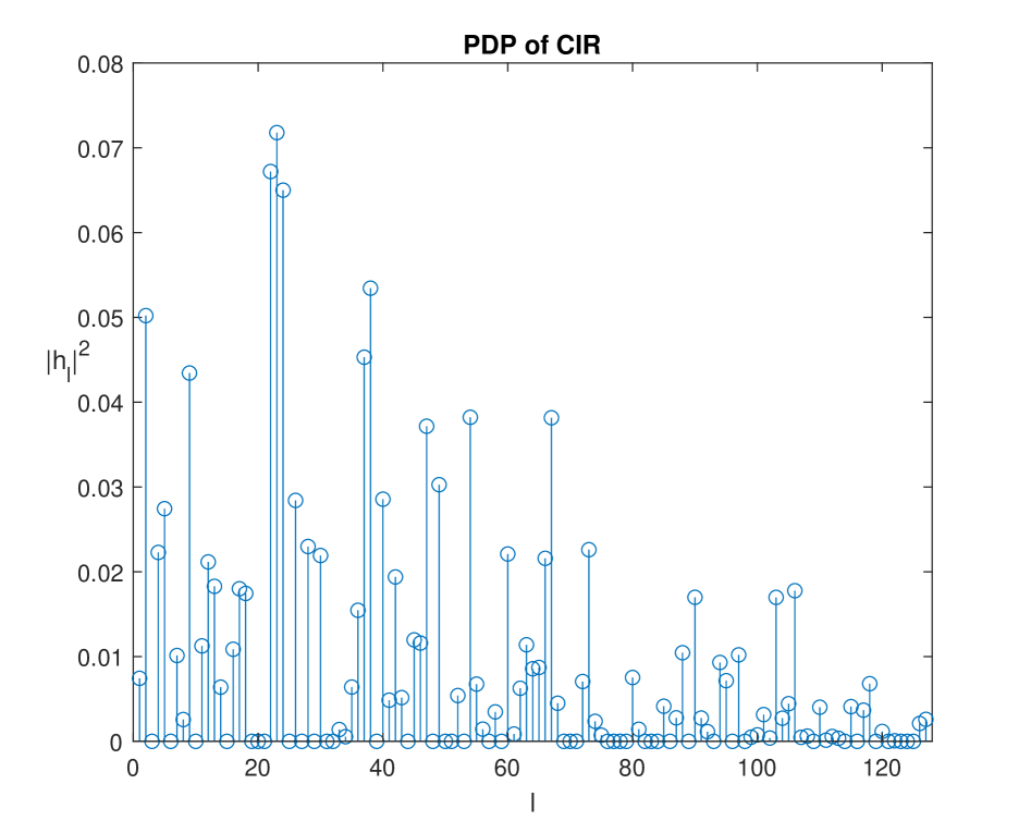
(a)

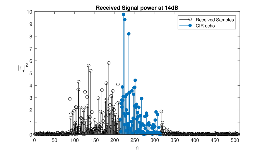
(b)

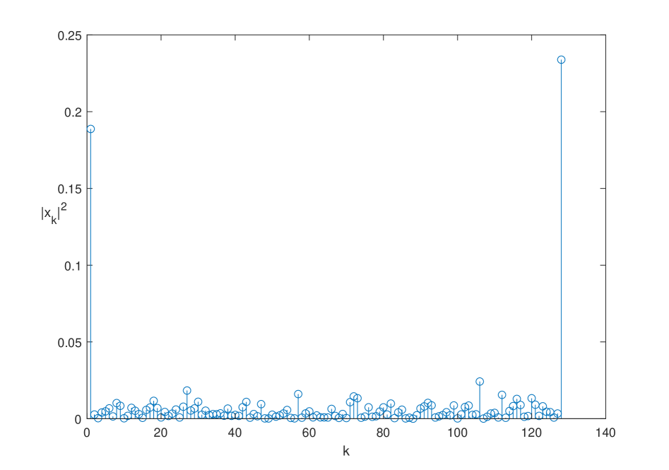
(c)

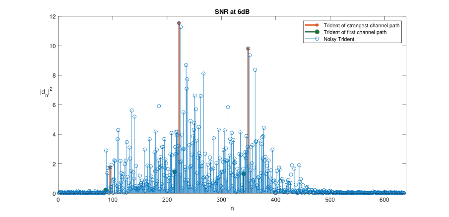
(d)

Figure 2: Absolute-squares of ((2(a))) a CIR realization with NLOS for $L=127,S=83,$ and $p=.98$ ((2(c))) normalized BMOCZ symbol with $K=127$ and $68$ outer zeros ((2(b))) received samples which echoes the distorted CIR with efficient length $L_{\text{eff}}=100$ and ((2(d))) the correlation of the received samples with the Huffman bracket at ${\text{rSNR}}=14dB$ with the echo of the trident multiplied by the strongest path in red and the first path in green at a timing-offset $\tau_{0}=86$.

IV Carrier Frequency Offset

Figure 3: Frequency-offset estimation via oversampling the DiZeT decoder for $K=6$ data zeros and without channel zeros by a factor of $Q=K=6$. Blue circles denote the codebook $\mathscr{Z}(6)$, solid blue circles the transmitted zeros $\boldsymbol{\alpha}_{k}$ and red the received rotated zeros $\tilde{\alpha}_{k}$.

We assume now, that the down-converted baseband signal in (9) has no further timing-offset and captured all path delays up to $N=K+L$. The signal will experience an unknown CFO of $\phi\in[0,2\pi)$

$$\tilde{y}_{n}=e^{jn\phi}({\mathbf{x}}*{\mathbf{h}})_{n}+w_{n}\quad,\quad n\in[N].$$ (27)

This is a common problem in many multi-carrier systems, such as OFDM, which therefore require CFO estimation algorithms [4, 6, 5]. For a bandwidth of $W=1/T$, the relative frequency offset is

$$\epsilon=\Delta f\cdot T=\Delta f/W.$$ (28)

Let us consider, for example, a carrier frequency of $f_{c}=1$GHz with a drastic frequency offset of $\Delta f\in[-1,1]$MHz and bandwidth $W=1$Mhz. This would result in a relative frequency offset $\epsilon\in[-1,1]$, which is able to rotate all zeros by any $\phi=2\pi\epsilon\in[0,2\pi)$ in the $z$-plane. Hence, the received polynomial (noiseless) will experience a rotation of all its $N-1$ zeros by the angle $\phi$

$$\tilde{{\mathrm{Y}}}(z) =\sum_{n=0}^{N-1}\tilde{y}_{n}z^{n}=\sum_{n=0}^{N-1}y_{n}e^{jn\phi}z^{n}={\mathrm{Y}}(e^{j\phi}z)=y_{N-1}\prod_{n=1}^{N-1}(e^{j\phi}z-\gamma_{n})$$ (29)

$$=e^{j\phi(N-1)}y_{N-1}\prod_{n=1}^{N-1}(z-\gamma_{n}e^{-j\phi})=e^{j\phi(N-1)}x_{K}h_{L-1}\prod_{k=1}^{K}(z-\alpha_{k}e^{-j\phi})\prod_{l=1}^{L-1}(z-\beta_{l}e^{-j\phi}).$$

As illustrated in Figure (3), we have to ensure that each rotated zero (red) $\tilde{\alpha}_{k}=e^{-j\phi}\alpha_{k}$ does not leave the zero-codebook set (blue) $\mathscr{Z}=\mathscr{Z}(K):=\left\{\left.R^{\pm 1}e^{j2\pi\frac{k}{K}}\rule[-2.5pt]{0.0pt}{10.0pt}\;\right|\;k\in[K]\right\}$. To apply the DiZeT decoder, we have to find $\theta$ such that $e^{j\theta}{\tilde{\boldsymbol{\alpha}}}\in\mathscr{Z}$, i.e., we need to ensure that all the $K$ data zeros will lie on the uniform grid. Hence, for $\theta_{K}=2\pi/K$ the CFO can be split in

$$\phi=l\theta_{K}+\theta$$ (30)

for some $l\in[K]$ and $\theta\in[0,\theta_{K})$, where $l$ is called the integer and $\theta$ the fractional CFO, which are also present in OFDM systems [9, Cha.5.2]. Only if $\theta=0$ (or correctly compensated), the DiZeT decoder, will sample at correct zero positions and decode, due to the unknown integer shift $l$, a cyclic permuted bit sequence $\tilde{\mathbf{m}}=\mathbf{m}\mathbf{S}^{l}$, which we will correct in Section (IV-C) by an cyclically permutable code.

IV-A Decoding BMOCZ via FFT

The DiZeT decoder for BMOCZ allows also a simple hardware implementation at the receiver. Let us scale the received samples $y_{n}$ with the radius powers $R^{n}$ respectively $R^{-n}$

$${\mathbf{y}}{\mathbf{D}}_{{\underline{\mathbf{R}}}}:={\mathbf{y}}\begin{pmatrix}1&0&\dots&0\\ 0&R&\dots&0\\[-5.0pt] \vdots&&\ddots&\vdots\\ 0&0&\dots&R^{N-1}\end{pmatrix}.$$ (31)

By applying the $\tilde{N}-$point unitary IDFT matrix ${\mathbf{F}^{*}}$ on the $N_{0}$ zero-padded scaled signal, where $\tilde{N}=QK$ with $Q:=\lceil N/K\rceil$, we get the samples of the $z-$transform by

$$\sqrt{N}{\mathbf{y}}\begin{pmatrix}{\mathbf{D}}_{{\underline{\mathbf{R}}}}&{\mathbf{0}}_{N,QK-N}\end{pmatrix}{\mathbf{F}^{*}}=\left(\sum_{n=0}^{N-1}y_{n}R^{n}e^{j2\pi\frac{0\cdot n}{\tilde{N}}},\dots,\sum_{n=0}^{N-1}y_{n}R^{n}e^{j2\pi\frac{(\tilde{N}-1)\cdot n}{\tilde{N}}}\right)={\mathrm{Y}}(\boldsymbol{\alpha}_{Q}^{(1)})$$

where $\alpha^{(m)}_{Q,k}=\alpha_{k}^{(m)}(e^{0},\dots,e^{j2\pi\frac{Q-1}{QK}})\in{\mathbb{C}}^{Q}$. Hence, the DiZeT decoder simplifies to

$$\hat{m}_{{k}}=\begin{cases}1&,|{\mathbf{y}}\tilde{{\mathbf{D}}}_{{\underline{\mathbf{R}}}}{\mathbf{F}^{*}}|_{Q(k-1)}<R^{K-1}|{\mathbf{y}}\tilde{{\mathbf{D}}}_{{\underline{\mathbf{R}}}^{-1}}{\mathbf{F}^{*}}|_{Q(k-1)}\\ 0&,\text{ else}\end{cases}\quad,\quad k=1,\dots,K.$$ (32)

Here, $Q\geq 2$ can be seen as an oversampling factor of the IDFT, where we pick each $Q$th sample point to obtain the zero sample values. Hence, the decoder can be fully implemented by a simple IDFT from the delayed amplified received signal, by using for example FPGA or even analog front-ends. We can also rewrite the diagonal scaling matrix (31) in the symmetric form

$${\mathbf{D}}_{R}:=\operatorname{diag}(R^{(N-1)/2},\dots,R^{-(N-1)/2})=R^{-(N-1)/2}{\mathbf{D}}_{{\underline{\mathbf{R}}}},$$ (33)

such that ${\mathbf{D}}_{R}^{-1}={\mathbf{D}}_{R^{-1}}$ corresponds to a time-reversal of the diagonal, which brings us to

$$|{\mathbf{y}}\tilde{{\mathbf{D}}}_{R}|_{Qk}{\mathbf{F}}^{*}_{QK}\leq|{\overline{{\mathbf{y}}^{-}}}\tilde{{\mathbf{D}}}_{R}{\mathbf{F}}^{*}_{QK}|_{Qk}\quad,\quad k\in[K],$$ (34)

since the absolute values cancel the phases from a circular shift $\mathbf{S}$ and the conjugate-time-reversal ${\overline{{\mathbf{y}}^{-}}}={\overline{{\mathbf{y}}}}\mathbf{S}\mathbf{\Gamma}$, where $\mathbf{\Gamma}={\mathbf{F}}^{2}$ is the circular time-reversal, can be rewritten by using ${\overline{{\mathbf{F}^{*}}\mathbf{\Gamma}}}={\overline{{\mathbf{F}}}}={\mathbf{F}^{*}}$.

IV-B Fractional CFO estimation via Oversampled FFTs

To estimate the factional frequency offset, we will oversample by choosing $Q>\lceil N/K\rceil$ to add $Q$ further $K$ zero blocks to ${\mathbf{D}}_{R}$. This leads to an oversampling factor of $Q$ and allows to quantize $[0,\theta_{K})$ in $Q$ uniform bins with separation $\phi_{Q}=\theta_{K}/Q$ for a base angle $\theta_{K}=2\pi/K$. Hence, the absolute values of the sampled $z-$transform in (27) of the rotated codebook-zeros are given by

$$|\tilde{{\mathrm{Y}}}(e^{jq\phi_{Q}}\alpha_{k}^{(1)})|=|\tilde{\mathbf{y}}\tilde{{\mathbf{D}}}_{R}{\mathbf{F}}^{*}_{QK}|_{Qk\oplus_{\tilde{N}}q}\quad,\quad|\tilde{{\mathrm{Y}}}(e^{jq\phi_{Q}}\alpha_{k}^{(0)})|=|{\overline{\tilde{\mathbf{y}}^{-}}}\tilde{{\mathbf{D}}}_{R}{\mathbf{F}}^{*}_{QK}|_{Qk\oplus_{\tilde{N}}q}$$ (35)

for each $q\in[Q]$ and $k\in[K]$, where $\oplus_{N}$ is addition modulo $N$. To estimate the fractional frequency offset of the base angle, we will sum the $K$ smaller sample values and select the fraction corresponding to the smallest sum

$$\hat{q} =\arg\min_{q\in[Q]}\sum_{k=1}^{K}\min\{|\tilde{\mathbf{y}}\tilde{{\mathbf{D}}}_{R}{\mathbf{F}}_{QK}|_{Qk\oplus_{\tilde{N}}q},|{\overline{\tilde{\mathbf{y}}^{-}}}\tilde{{\mathbf{D}}}_{R}{\mathbf{F}}_{QK}|_{Qk\oplus_{\tilde{N}}q}\}\quad\text{ and }\quad\hat{\theta}=\frac{\hat{q}}{Q}\theta_{K}.$$ (36)

Then the recovered signal ${\hat{\mathbf{y}}}=\tilde{\mathbf{y}}\mathbf{M}^{-\hat{\theta}}$ will have the data zeros on the constellation grid $\mathscr{Z}_{K}$. See Figure (4) for a random fractional CFO $\theta$ and Figure (3) for a schematic picture.

Figure 4: BER over rSNR for BMOCZ with DiZeT for random $\phi\in[0,\theta_{K}/2)$ for $L=K=32$.

IV-C Using Cyclically Permutable Codes

To be robust against rotations which are integer multiple of the base angle, we will need an outer block code in $\mathbb{F}_{2}^{K}$ for the binary message $\mathbf{m}\in\mathbb{F}_{2}^{B}$, which is invariant against cyclic shifts, i.e., a bijective mapping on the Galois Field $\mathbb{F}_{2}=\{0,1\}$

$$\mathcal{G}\colon\mathbb{F}_{2}^{B}\to\mathbb{F}_{2}^{K},\mathbf{m}\mapsto{\mathbf{c}}=\mathcal{G}(\mathbf{m})$$ (37)

such that $\mathcal{G}^{-1}({\mathbf{c}}\mathbf{S}^{l})=\mathbf{m}$ for any $l\in[K]$. We will use the common notation for the code length $n=K$. Such a block code is called a cycling register code (CRC) $\mathscr{C}_{\text{CR}}$ [22], which can be constructed from the linear block code $\mathbb{F}_{2}^{n}$, by separating it in all its cyclic equivalence classes

$$[{\mathbf{c}}]_{\text{CRC}}=\left\{\left.{\mathbf{c}}\mathbf{S}^{l}\rule[-2.5pt]{0.0pt}{10.0pt}\;\right|\;l\in[n]\right\}\quad,\quad{\mathbf{c}}\in\mathbb{F}_{2}^{n}$$ (38)

where ${\mathbf{c}}$ has cyclic order $\nu$ if ${\mathbf{c}}\mathbf{S}^{\nu}={\mathbf{c}}$ for the smallest possible $\nu\in\{1,2,\dots,n\}$. To make coding one-to-one, each equivalence class can be represented by the codeword $\tilde{\mathbf{c}}$ with smallest decimal value [23]. Then $\mathbb{F}_{2}^{n}$ is given by the union of all its equivalence class representatives and its cyclic shifts, i.e.

$$\mathbb{F}_{2}^{n}=\bigcup_{i=1}^{M_{\text{CRC}}}\left\{\left.\tilde{\mathbf{c}}_{i}\mathbf{S}^{l}\rule[-2.5pt]{0.0pt}{10.0pt}\;\right|\;l=1,\dots,\nu(i)\right\}$$ (39)

This will generate in a systematically way a look-up table for the cycling register code. Unfortunately, the construction is non-linear and combinatorial difficult. However, the cardinality of such a code is proven explicitly for any positive integer $n$ in [22, Thm.VI.3] to be (number of cycles in a cycling register)

$$|\mathscr{C}_{\text{CR}}(n)|=\frac{1}{n}\sum_{d|n}\Phi(d)2^{n/d}$$ (40)

where $\Phi(d)$ is the Euler function, which counts the number of elements $t\in[d]$ coprime to $d$. For $n$ prime, we obtain

$$|\mathscr{C}_{\text{CR}}(n)|=\frac{1}{n}(2^{n}+(n-1)2)\geq\frac{2^{n}}{n}=2^{n-\log_{2}n}$$ (41)

which would allow to encode at least $B=n-\lceil\log n\rceil$bits. For $n=K=31$ this would result in a loss of only $5$bits and is similar to the loss in a BCH-$(31,26)$ code, which can correct $1$bit error. Note, the cardinality of a cycling register code $\mathscr{C}_{\text{CR}}$ is minimal if $n$ is prime. This can be seen by acknowledging the fact that the cyclic order of a codeword is always a divisor of $n$, see for example [24, Lem.1]. Therefore, if $n$ is prime we only have the trivial orders $1$ and $n$, where the only codewords with order $\nu=1$ are the all one ${\mathbf{1}}$ and all zero ${\mathbf{0}}$ codeword and all other codewords have the maximal or full cyclic order $\nu=n$. Hence, extracting the CRC from $\mathbb{F}_{2}^{n}$ obtains the same cardinality (41). Taking from a block code of length $n$ only the codewords of maximal cyclic order and selecting only one representative of them defines a cyclically permutable code (CPC) and was first introduced by Gilbert in [27]. If $n$ is prime, only two equivalence classes in $\mathscr{C}_{\text{CR}}$ are not of maximal cyclic order, hence the cardinality for a CPC if $n$ is prime is at most $(2^{n}-2)/n$.

However, the construction from $\mathbb{F}_{2}^{n}$, even for $n$ prime, is a combinatorial problem, especially the decoding. Hence, to reduce the combinatorial complexity, many approaches starting from cyclic codes and extract all codewords with maximal cyclic order [28, 29, 30]. Since a cyclic $(n,k,{d_{\text{\rm min}}})$ code corrects up to $({d_{\text{\rm min}}}-1)/2$ bit errors, any CPC code extraction will inherit the error correction capability.

We will follow an approach from [28] to construct a CPC from a binary cyclic $(n,k,{d_{\text{\rm min}}})$ code by still obtaining the best possible cardinality $(2^{k}-2)/n$ if $n$ is a Mersenne prime. By reasons which will be clear later, we can extract from this CPC an affine subcode whith maximal dimension, which we will call an affine cyclically permutable code (ACPC). This allows a linear encoding of $B=n-\lfloor\log n\rfloor$ bits by a generator matrix and an additive non-zero row vector, which defines the affine translation.

IV-C1 CPC construction from cyclic codes

Cyclic codes exploit efficiently the algebraic structure of Galois fields $\mathbb{F}_{q}$, given by a finite set having a prime power cardinality $q=p^{m^{\prime}}$. A linear block code over $\mathbb{F}_{q}$ is a cyclic code if each cyclic shift of a codeword is a codeword. It is a simple-root cyclic code if the characteristic $p$ of the field $\mathbb{F}_{q}$ is not a divisor of the block length $n$. If the block length is of the form $n=q^{m}-1$, we call it a primitive block length and if the code is cyclic we call it a primitive cyclic code, [31, Def.5.3.1]. We will investigate here binary cyclic codes of length $n=2^{m}-1$ with $q=p=2$, which are simple-root and primitive cyclic codes. Due to its linearity, cyclic codes can be encoded and decoded by a generator ${\mathbf{G}}$ and check matrix $\mathbf{H}$ in a systematic way. The cardinality of a binary cyclic $(n,k)$ code is always $M_{c}=2^{k}$. Hence, by partitioning the cyclic code in equivalence classes of maximal cyclic order and selecting one codeword as their representative leaves us with a maximal cardinality of

$$|\mathscr{C}_{\text{CPC}}|\leq\frac{2^{k}-1}{n}.$$ (42)

for any extracted CPC. Note, the zero codeword is always a codeword in a linear code but has cyclic order one and hence is not an element of a CPC. To exploit the cardinality most efficiently, the goal is to find cyclic codes such that each non-zero codeword has maximal cyclic order. We will follow a construction of Kuribayashi and Tanaka in [28] for prime code lengths of the form $n=2^{m}-1$, also known as Mersenne primes. For $m=2,3,5,7$ this applies to $K=n=3,7,31,127$, which are relevant signal lengths for binary short-messages. Furthermore, we will only consider cyclic codes which have ${\mathbf{1}}$ as a codeword. We will show later that this is indeed the case. Since $n$ is prime, each codeword, except ${\mathbf{0}}$ and ${\mathbf{1}}$ has maximal cyclic order. Hence, each codeword of a cyclic $(n,k)$ code has maximal cyclic order and since it is a cyclic code all its cyclic shifts must be also codewords. Hence the cardinality of codewords having maximal order is exactly $M=2^{k}-2$. Therefore, we only need to partition the cyclic code in its cyclic equivalence classes, which will leave us with $|\mathscr{C}_{\text{CPC}}|=M/n=(2^{k}-2)/n$. Note, this number must be indeed an integer, by the previous mentioned properties, see also [28, Lem.2]. The main advantages of the Kuribayashi-Tanaka (KT) construction is the systematic code construction and the inherit error-correcting capability of the underlying cyclic code, from which the CPC is constructed. Furthermore, combining error-correction and cyclic-shift corrections will be ideal for BMOCZ.

The code construction is two-folded. We have an inner $\mathscr{C}_{\text{in}}-(k,k-m)$ and outer $\mathscr{C}_{\text{out}}-(n,k)$ cyclic code, where the inner cyclic codewords will be affine translated by the Euclidean vector ${\mathbf{e}}_{1}=(1,0,\dots,0)\in\mathbb{F}_{2}^{k}$. In this sense, the CPC construction is affine. This can be realized by an affine mapping from $\mathbb{F}_{2}^{k-m}$ to $\mathbb{F}_{2}^{n}$, which can be represented by the BCH generator matrices ${\mathbf{G}}_{\text{in}}$ and ${\mathbf{G}}_{\text{out}}$ together with the affine translation ${\mathbf{e}}_{1}$ as

$$\begin{split}\mathcal{G}\colon\mathbb{F}_{2}^{k-m}&\to\mathscr{C}_{\text{in}}+{\mathbf{e}}_{1}\to\mathscr{C}_{\text{out}}\subset\mathbb{F}_{2}^{n}\\ \mathbf{m}&\mapsto{\mathbf{i}}=\mathbf{m}{\mathbf{G}}_{\text{in}}+{\mathbf{e}}_{1}\mapsto{\mathbf{c}}={\mathbf{i}}{\mathbf{G}}_{\text{out}}=\mathcal{G}(\mathbf{m}).\end{split}$$ (43)

To derive the generator matrix we can exploit the algebraic structure of the cyclic codes, given by its Galois fields. By definition of cyclic codes, we have to factorize the polynomial

$$x^{n}-1=(x-1)\prod_{s=1}^{S}{\mathrm{G}}_{s}(x)$$ (44)

in irreducible polynomials ${\mathrm{G}}_{s}(x)$ of degree $m_{s}$, which must be divisors of $m$. If $n$ is prime, $m$ must be also prime and hence all the irreducible polynomials are primitive and of degree $m_{s}=m$, except one of them, ${\mathrm{G}}_{0}(x)=x-1$, has degree one. Hence, it must hold $S=(n-1)/m$. As outer generator polynomial ${{\mathrm{G}}}_{\text{out}}(x)=\prod_{s=S-J+1}^{S}{\mathrm{G}}_{s}(x)=\sum_{i=0}^{Jm}g_{\text{out},i}x^{k}$ we choose the product of the last $1\leq J\leq S$ primitive polynomials ${\mathrm{G}}_{s}(x)$ yielding to a degree $Jm=n-k$, see [28, (23)]. Each codeword polynomial of degree less than $n$ is then given by

$${\mathrm{C}}(x)={\mathrm{I}}(x){{\mathrm{G}}}_{\text{out}}(x)$$ (45)

where ${\mathrm{I}}(x)=\sum_{a=0}^{k-1}i_{a}x^{a}$ is the informational polynomial of degree less than $k$ and represented by the binary information word ${\mathbf{i}}=(i_{0},i_{1},\dots,i_{k-1})\in\mathbb{F}_{2}^{k}$, which we call the inner codeword. Similar, the codeword polynomial ${\mathrm{C}}(x)$ is represented by the CPC codeword ${\mathbf{c}}\in\mathbb{F}_{2}^{n}$. By [28, Thm.2] a message polynomial ${\mathrm{M}}(x)=\sum_{b=0}^{k-m-1}m_{b}x^{b}$ of degree less than $k-m$ and ${\mathrm{R}}(x)=1$ will be mapped to the information polynomial by the inner generator polynomial

$${\mathrm{I}}(x) ={\mathrm{M}}(x){{\mathrm{G}}}_{\text{in}}(x)+1.$$ (46)

In [28] the authors map all possible cyclic equivalence classes to ${\mathrm{M}}(x)$, by separating the inner code in $S-1$ separated inner codes. However, the remaining $S-2$ codes will only map $<2^{k-m}$ more message polynomials to codeword polynomials and therefore be not enough to encode an additional bit. Hence, we will just omit these other inner codewords. This has the advantage, that we can write with (43) the subset of the CPC as an affine cyclically permutable code (ACPC), which is given by the polynomial multiplication over $\mathbb{F}_{2}$

$${\mathrm{C}}(x) ={\mathrm{I}}(x){{\mathrm{G}}}_{\text{out}}(x)=({\mathrm{M}}(x){{\mathrm{G}}}_{\text{in}}(x)+1){{\mathrm{G}}}_{\text{out}}(x)={\mathrm{M}}(x){\mathrm{G}}(x)+{{\mathrm{G}}}_{\text{out}}(x).$$ (47)

Here, we introduced a third generator polynomial ${\mathrm{G}}(x)={{\mathrm{G}}}_{\text{in}}(x){{\mathrm{G}}}_{\text{out}}(x)$ which will be affine translated by the polynomial ${{\mathrm{G}}}_{\text{out}}(x)$. This generator polynomial ${\mathrm{G}}(x)$ will map surjective $\mathbb{F}_{2}^{k-m}$ to a cyclic code in $\mathbb{F}_{2}^{n}$ and can therefore be expressed in matrix form as

$$\mathbf{m}{\mathbf{G}}+{\mathbf{g}}_{\text{out}}\in\mathscr{C}_{\text{ACPC}}\subset\mathscr{C}_{\text{out}}$$ (48)

where ${\mathbf{g}}_{\text{out}}=(g_{\text{out},0},\dots,g_{\text{out},n-k},0,\dots,0)\in\mathbb{F}_{2}^{n}$ and the generator matrix (Toeplitz) is given by

$${\mathbf{G}} =\begin{pmatrix}g_{0}&g_{1}&\dots&g_{k-(k-m)-1}&g_{k-(k-m)}&0&\dots&0\\ 0&g_{1}&\dots&g_{k-(k-m)-2}&g_{k-(k-m)-1}&g_{k-(k-m)}&\dots&0\\ |&\vdots&&&&&\diagdown&\vdots\\ 0&0&\dots&&&&\dots&g_{m}\end{pmatrix}\in\mathbb{F}_{2}^{k-m\times k}.$$ (49)

For linear codes, we can use the Euclidean algorithm, to compute $x^{n-i}=Q_{i}(x){\mathrm{G}}(x)+{\mathrm{S}}_{i}(x)$ for $i=1,\dots,k-m$, where the remainder polynomials ${\mathrm{S}}_{i}(x)=\sum_{j}s_{i,j}x^{j}$ will have degree less than $n-k=n-(n-m)=m$, which allows one to rewrite the Toeplitz matrices as systematic matrices, see [31, pp.112]. Here, the check symbols $s_{i,j}$ define the $k-m\times n$ systematic generator and $n\!-\!k\!+\!m\times n$ check matrix

$${\tilde{\mathbf{G}}}\!=\![-\mathbf{P}\ {\mathbf{I}}_{k-m}],\ {\tilde{\mathbf{H}}}\!=\![{\mathbf{I}}_{n-k+m}\ \mathbf{P}^{T}]\text{ with }\mathbf{P}\!=\!\begin{pmatrix}s_{k-m,0}&\dots&s_{k-m,n-k-1}&{\mathbf{0}}_{m}\\ s_{k-m-1,0}&\dots&s_{k-m-1,n-k-1}&{\mathbf{0}}_{m}\\ \vdots&&\vdots&\vdots\\ s_{1,0}&\dots&s_{1,n-k-1}&{\mathbf{0}}_{m}\end{pmatrix}$$ (50)

such that ${\tilde{\mathbf{G}}}{\tilde{\mathbf{H}}}^{T}={\mathbf{O}}_{k-m,n-k+m}$. Here we needed zero padding to embed the code in $\mathbb{F}_{2}^{n}$. This allows one to write the cyclic outer code as $\mathbb{F}_{2}^{k-m}{\mathbf{G}}=\mathbb{F}_{2}^{k-m}{\tilde{\mathbf{G}}}$. Of course, each $\mathbf{m}{\mathbf{G}}$ and $\mathbf{m}{\tilde{\mathbf{G}}}$ will be mapped to different codewords, but this is just a relabeling. Since $\mathbb{F}_{2}^{k-m}{\tilde{\mathbf{G}}}$ defines a cyclic $(n,k-m)$ code and $n$ is prime, each codeword must have $n$ distinct cyclic shifts. The affine translation ${\mathbf{g}}_{\text{out}}$ separates than each of these $n$ distinct cyclic shifts by mapping them to representatives of distinct cyclically equivalence classes of maximal order. This gives us a very simple encoding rule for each $\mathbf{m}\in\mathbb{F}_{2}^{B}$:

$${\mathbf{c}}=\mathbf{m}{\tilde{\mathbf{G}}}+{\mathbf{g}}_{\text{out}}=\mathcal{G}(\mathbf{m})\in\mathscr{C}_{\text{ACPC}},$$ (51)

and decoding rule. Here an ACPC codeword ${\mathbf{c}}$ can be decoded by just subtracting the affine translation ${\mathbf{g}}_{\text{out}}$ and cut-off the last $B=k-m$ binary letters to obtain the message word $\mathbf{m}\in\mathbb{F}_{2}^{B}$, see (50). However, we will observe a cyclic shifted codeword ${\mathbf{v}}={\mathbf{c}}\mathbf{S}^{l}$ and by construction we know that only one cyclic shift will be an element of $\mathscr{C}_{\text{ACPC}}$ and consequently it holds

$$\;\forall\;j\not=l\mod(n-1)\colon\tilde{\mathbf{c}}_{j}={\mathbf{v}}\mathbf{S}^{-j}-{\mathbf{g}}_{\text{out}}\not\in\mathbb{F}_{2}^{k-m}{\tilde{\mathbf{G}}}\quad\Leftrightarrow\quad\tilde{\mathbf{c}}_{j}{\tilde{\mathbf{H}}}^{T}\not={\mathbf{0}}.$$ (52)

Hence, we only need to check all $n$ cyclic shifts of the sense-word ${\mathbf{v}}$ to identify the correct cyclic shift $l$, which is given if $\tilde{\mathbf{c}}_{l}{\tilde{\mathbf{H}}}^{T}={\mathbf{0}}$. If there is an additive error ${\mathbf{e}}$ we can use the error correcting property of the outer cyclic code $\mathscr{C}_{\text{out}}$in (47) to repair the codeword. Here, we can use again the systematic matrices ${\mathbf{\widetilde{G}}}_{\text{out}}$ and ${\mathbf{\tilde{H}}}_{\text{out}}$ to represent the outer cyclic code in a systematic way. Note, that each information message ${\mathbf{i}}$ which corresponds to a CPC codeword ${\mathbf{c}}$ will be an element of $\mathbb{F}_{2}^{k}{\mathbf{\widetilde{G}}}_{\text{out}}$. Furthermore, all its cyclic shifts ${\mathbf{c}}\mathbf{S}^{l}$ will be outer cyclic codewords. Hence, by observing the sense-word

$$\tilde{\mathbf{v}}={\mathbf{c}}\mathbf{S}^{l}+{\mathbf{e}}$$ (53)

and determining its syndrome ${\mathbf{s}}={\mathbf{v}}{\mathbf{\tilde{H}}}_{\text{out}}^{T}$, which we look-up int the syndrome table $\mathbf{T}_{\text{synd}}$ of ${\mathbf{\tilde{H}}}_{\text{out}}$ to identify the corresponding coset leader (error-word) ${\mathbf{e}}$, which recovers the shifted codeword (we assume maximal $t$ errors, bounded-distance decoder) as

$${\mathbf{v}}=\tilde{\mathbf{v}}-{\mathbf{e}},$$ (54)

see for example [31, p.59]. This allows to correct up to $t=(n-k-1)/2$ errors of the cyclic codeword. From the additive error-free sense-word ${\mathbf{c}}$ we can, as described previously, identify the correct shift $\hat{l}$ from (52) and by taking the last $B=k$ letters the original message $\mathbf{m}$. If the error vector ${\mathbf{e}}$ introduces more than $t$ bit flips, the error correction will fail and the chance is high that we will mix up the ACPC codewords and experience a block (word) error. Therefore, we will need low coding rates for the outer cyclic code ${\mathbf{G}}_{\text{out}}$ to prevent such a catastrophic error. The identified cyclic shift and fractional CFO estimation (36) yields then the estimated CFO

$$\hat{\phi}=\hat{\theta}+\hat{l}\theta_{K}.$$ (55)

Example 1. The most non-trivial example of ACPC is for $m=3$ and $l=1$, which gives

$$n=2^{3}-1=7,\quad k=7-3=4,\quad B=4-1=1$$ (56)

This is also the Hamming $(7,4)$ code with minimal distance ${d_{\text{\rm min}}}=3$ and hence can correct $1$ bit error. The code is also perfect.

Example 2. For $K=n=31$ we get for $t=2$ error corrections a message length of $k=21$ in a cyclic BCH-$(31,21)$ code from which we can construct a CPC of cardinality [28, (25),(30)]

$$|\mathscr{C}_{\text{CPC}}|=\sum_{i=1}^{4}2^{5(i-1)+1}=2^{1}+2^{6}+2^{11}+2^{16}=6750\geq 2^{16}.$$ (57)

This allows to encode $B=16=k-m$bits. The cardinality is optimal for any cyclic $(31,26)$ code (42)

$$|\mathscr{C}_{\text{CPC}}|=\frac{M_{c}}{n}=\frac{2^{21}-2}{31}=2\frac{2^{20}-1}{2^{5}-1}=\sum_{i=0}^{3}2^{5i+1}=2^{1}+2^{6}+2^{11}+2^{16}=6750.$$ (58)

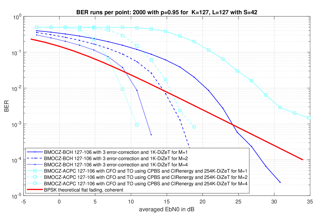
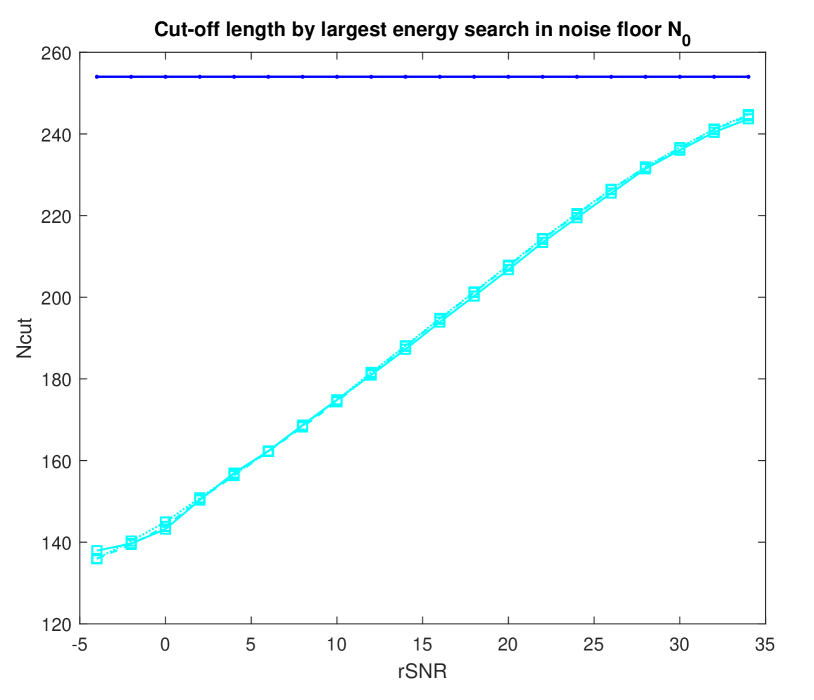
Figure 7: SIMO for $M=1,2,4$ receive antennas over $2$k runs per point at $p=0.95$ and $S=42$. BCH with no CFO and TO and ACPC with CFO and TO using Algorithm (1)+(2).

The next example would be for $n=127$, which we also simulated in Figure (7). Unfortunately, the next Mersenne prime is only at $8191$, which might be not anymore considered as a short-packet length. However, the authors want to emphasize that other CPC constructions exist which do not require Mersenne prime lengths $n$ or even binary alphabets. In [30] the authors showed construction of CPCs with alphabet size $q$, given as a power of a prime, and block length $n=q^{m}-1$ for any positive integer $m$. Hence, for $q=2$ and a binary cyclic code $(n=2^{m}-1,k,{d_{\text{\rm min}}})$ which satisfy [30, Thm.1] will result in $(2^{k}-1)/n$ CPC codewords. An example is given for $n=15=2^{4}-1$ and $k=8,{d_{\text{\rm min}}}=4$ where $n$ is not a Mersenne prime number and the maximal bound (42) of $(2^{8}-1)/15=17$ is achieved, allowing to encode $B=4$ bits and correct $2$ bit errors. which is very close to the BCH code $(15,7)$ with $2$bit error correction.

Let us mention the shortest non-trivial CPC, which can be addressed without cyclic code construction, but also with no error correction capabilities.

Example 3. For $n=3$ we get only have $2^{3}=8$ binary words of length $3$ which have $4$ different cyclic permutable codewords ${\mathbf{c}}_{1}={\mathbf{1}},{\mathbf{c}}_{2}=(1,1,0),\ {\mathbf{c}}_{3}=(1,0,0),\ {\mathbf{c}}_{4}={\mathbf{0}}$ allowing to encode $B=2$bits of information with no error correction. However, this code allows an TO estimation, as well as a CIR estimation. For a super short control signal, this might be therefore interesting. By omitting ${\mathbf{c}}_{1}$ and ${\mathbf{c}}_{4}$, i.e., by dropping one bit of information, we can even estimate with the DiZeT oversampling decoder any possible CFO.

V Simulations

We determined by Monte-Carlo simulations with MatLab 2017a the bit-error-rate (BER) over averaged ${E_{\text{b}}/N_{0}}$ and rSNR under various channel settings and block lengths $K$. The transmit and receive time will be in all schemes $N=K+L$ over which the CIR ${\mathbf{h}}$ of length $L$ is assumed to be static, see Figure (9). Therefore, the energy per bit is $E_{b}=B/N$ with $B=\left\|\mathbf{m}\right\|_{1}$ which is the inverse of the spectral efficiency $\rho=N/B$. In each simulation run, the CIR coefficients are redrawn according to the channel statistic given by the decay exponent $p\leq 1$. The CFO $\phi$ is drawn uniformly from $[0,2\pi)$ and the timing-offset $\tau_{0}$ uniformly form $[0,N]$. Furthermore, the additive distortion is also drawn from an i.i.d. Gaussian distribution $\mathcal{CN}(0,N_{0})$, which we will scale to obtain various received SNR and ${E_{\text{b}}/N_{0}}$ values, Figure (5(a)).

Due to the embedded error correcting and a complete failure if a wrong CPC codeword is detected, the BER and BLER (block-error-rate) are almost identical over received SNR for BMOCZ-ACPC, see Figure (5(b)).

Of course, it would be also possible to detect a wrong decoding and request a retransmit. However, this is in contrast to our system aspects since we want to address sporadic communication of single packets.

V-A Multiple Receive Antennas

For a receiver with $M$ antennas, we may exploit receive antenna diversity, since each antenna will receive the transmit signal over an independent CIR realization (best case). Due to the short wavelength in the mmWave band large antenna arrays with $\lambda/2$ spacing can be easily installed on small devices. We assume in all simulations:

• The $B$ information bits $\mathbf{m}\in\mathbb{F}_{2}^{B}$ are drawn uniformly.

• All signals arrive with the same timing-offset $\tau_{0}$ at the $M$ receive antennas (dense antenna array, fixed relative antenna positions (no movements)).

• The clock-rate for all $M$ antennas is identical, hence all received signals have same CFO.

• The maximal CIR length $L$, sparsity level $S$, and PDP $p$ are the same for all antennas.

• Each received signal experience an independent noise and CIR realization, with sparsity pattern ${\mathbf{s}}_{m}\in\{0,1\}^{L}$ for $|{\operatorname{supp}({\mathbf{s}}_{m})}|=S$ and ${\mathbf{h}}_{m}\in{\mathbb{C}}^{L}$ where $h_{m,l}=\mathcal{CN}(0,s_{m,l}p^{l})$.

The DiZeT decoder (32) for BMOCZ without TO and CFO, can be implemented straight forward to a single-input-multiple-output SIMO antenna system:

$$\hat{m}_{{k}}=\begin{cases}1&,\sum_{m=1}^{M}|{\mathbf{y}}_{m}\tilde{{\mathbf{D}}}_{{\underline{\mathbf{R}}}}{\mathbf{F}^{*}}|^{2}_{Q(k-1)}<R^{2K-2}\sum_{m=1}^{M}|{\mathbf{y}}_{m}\tilde{{\mathbf{D}}}_{{\underline{\mathbf{R}}}^{-1}}{\mathbf{F}^{*}}|^{2}_{Q(k-1)}\\ 0&,\text{ else}\end{cases}.$$ (59)

V-B CFO Estimation for Multiple Receive Antennas

As in Section (IV-B) we can estimate the fractional CFO by (36) for $M$ received signals ${\mathbf{y}}_{m}$

$$\hat{q}=\arg\min_{q\in[Q]}\sum_{k=1}^{K}\min\left\{\sum_{m=1}^{M}|\tilde{\mathbf{y}}_{m}\tilde{{\mathbf{D}}}_{R}{\mathbf{F}}_{QK}|_{Qk\oplus_{\tilde{N}}q},\sum_{m=1}^{M}|{\overline{\tilde{\mathbf{y}}^{-}}}_{m}\tilde{{\mathbf{D}}}_{R}{\mathbf{F}}_{QK}|_{Qk\oplus_{\tilde{N}}q}\right\}.$$ (60)

The effect of different coding rates on BER and block error rate (BLER) for the BMOCZ-ACPC-$(K,B)$ scheme with $K=31$ transmitted zeros and channel lengths $L=16,32$ with flat power profile $p=1$ is shown in Figure (5). If the coding rate is decreased to $B/K=6/31\simeq 1/5$, allowing up to $5$ bit error corrections, we achieve a BLER of $10^{-1}$ at almost $6$dB received SNR, which is $6$dB better as for the coding rate $16/31\simeq 1/2$. Hence, if power is an issue, the coding rate can be decreased accordingly to approach a low SNR regime, at the cost of data rate.

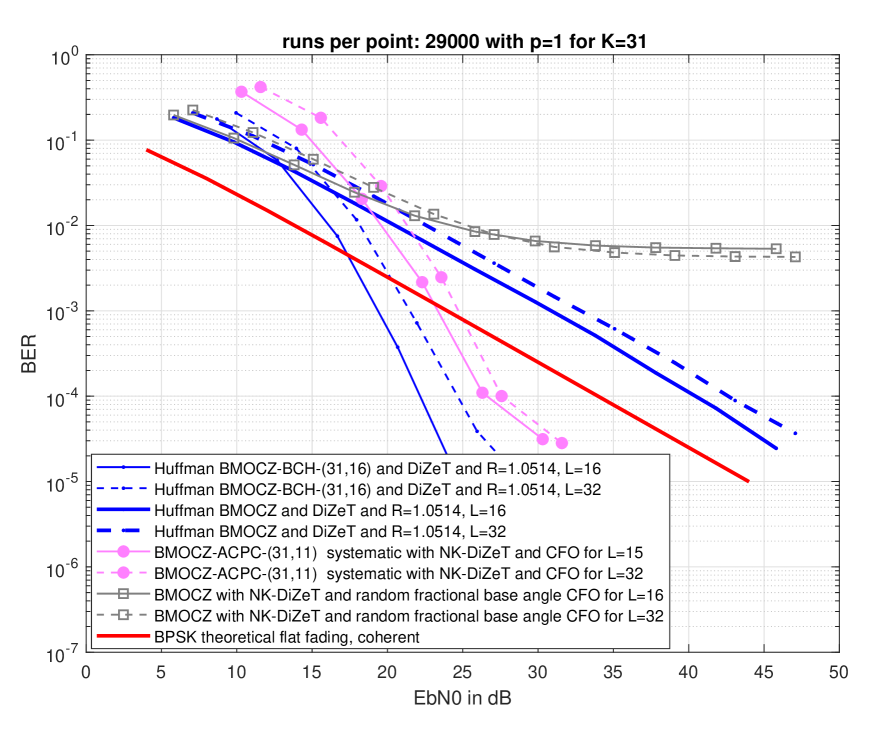
(a)

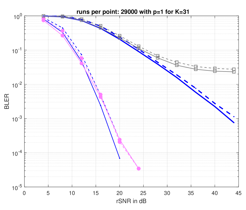
(b)

Figure 5: Simulations for arbitrary CFO with ACPC-(31,11) for $B=11$bits. The $E_{b}/N_{0}$ averaged over the fading channel is defined here as $1/BN_{0}$ for $B$ information bits.

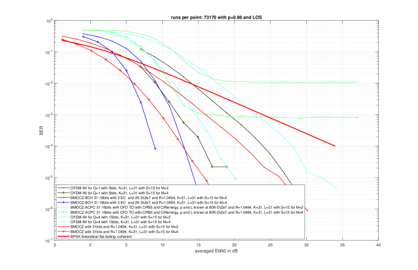
Figure 6: BER over $E_{\text{b}}/N_{0}$ with $M=2$ and $4$ antennas for BMOCZ-ACPC-$(31,16)$ distorted by TO and CFO (green curves). OFDM-IM is without CFO and TO.

V-C Timing and Effective Channel Length Estimation

We chose a random integer timing offset in $\tau_{0}\in\{0,1,2\dots,N-1\}$ in Figure (6) and with an exponentially power delay profile exponent $p=0.98$ and dominant LOS path. In the CPBS Algorithm (1) and CIRenergy Algorithm (2) we used the sum of all received antenna samples and the sum of the noise powers

$$|r_{n}|^{2}=\sum_{m=1}^{M}|r_{m,n}|^{2}\quad\text{ and }\quad\sigma^{2}=MN_{0}.$$ (61)

Indeed, if the CIR length is larger with exponential decay, a wrong TO estimation yields to less performance degradation as for shorter lengths, since the last channel tap will be much smaller in average power. We simulated by choosing randomly for each simulation, consisting of $D$ different noise powers $N_{0}$, Each binary plain message $\mathbf{m}$ will result in a codeword ${\mathbf{c}}\in\mathbb{F}_{2}^{K}$ which corresponds to a normalized BMOCZ symbol ${\mathbf{x}}\in{\mathbb{C}}^{K+1}$. We will normalize the CIR at the transmitter to $\tilde{\mathbf{h}}={\mathbf{h}}/{\mathbb{E}[\left\|{\mathbf{h}}\right\|^{2}]}$, where the average energy of the CIR is given by (24) as the expected power delay profile in ${\mathbf{s}}$

$$E_{S,h}={\mathbb{E}[\left\|{\mathbf{h}}\right\|^{2}]}=\sum_{l=0}^{L-1}s_{l}p^{l}.$$ (62)

This ensures that for each selected sparsity pattern of the CIR, we will have normalized CIR energy if selecting random channel taps by the law of large numbers. By averaging over the sparsity pattern, this would result in a large deviation of the CIR energy and would require many more simulations, therefore we calculated the average power with knowledge of the sparsity patterns, i.e., by knowing the support realization.

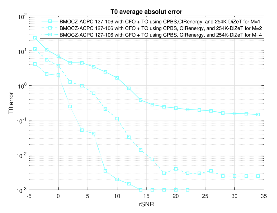
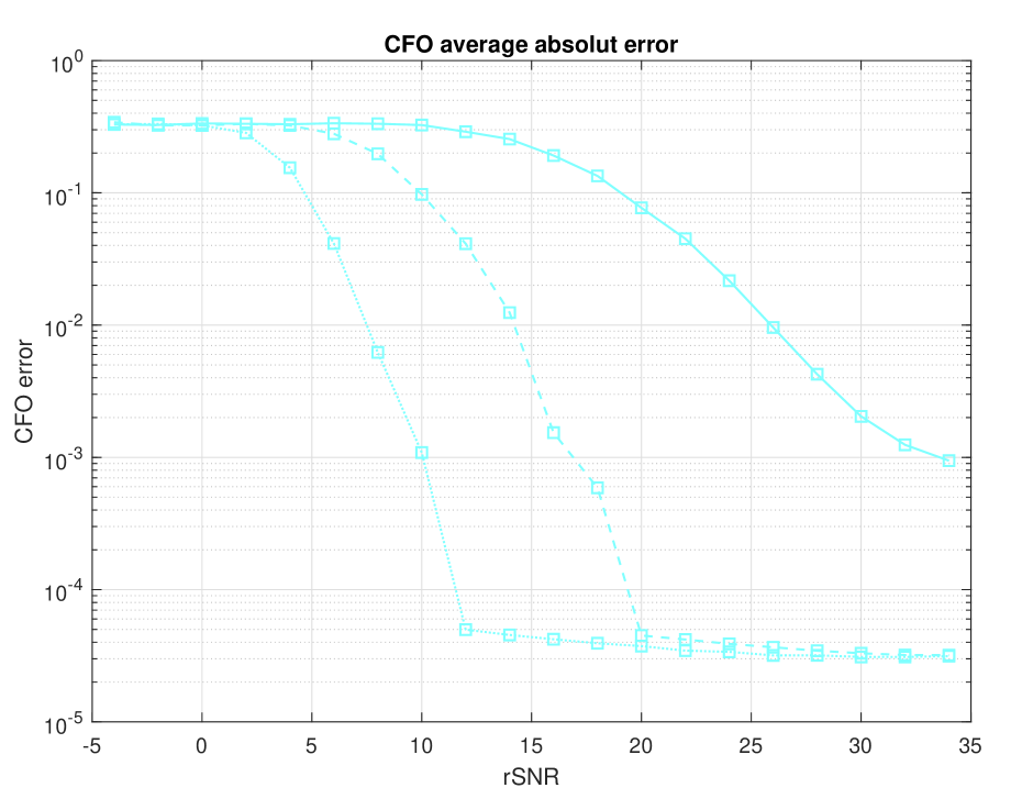
Figure 8: TO and CFO estimation errors for $M=1,2$ and $M=4$ receive antennas.

V-D Comparison to Noncoherent Schemes

First, we will compare without TO and CFO BMOCZ to OFDM and pilot based schemes, as in [2], in Figure (10(b)) with a single antenna where the CIR is generated from the simulation framework Quadriga [13] and finally in Figure (11(a)) with multiple-receive antennas.

Pilot and SC-FDE with QPSK

Here we use a pilot impulse $\sqrt{\frac{E}{2}}\boldsymbol{\delta}_{0}$ of length $P=L$ to determine the CIR and $K+1-L$ symbols to transmit data via QPSK in a single-carrier (SC) modulation by a frequency-domain-equalization (FDE). Applying FDE, we can then decode the QPSK or QAM modulated OFDM subcarriers $K+1-L$, see [1]. The energy $E$ is split evenly between the pilots and data symbols, which results in better BER performance for high SNR, see Figure (11(b)) (we not use SNR knowledge at the transmitter)

OFDM-Index-Modulation (IM)

We also compare to: OFDM-IM with $Q=1$ and $Q=4$ active subcarriers out of $K_{\text{IM}}={K}+1$ and to OFDM-Group-Index-Modulation (GIM) with $Q=1$ active subcarriers in each group of size $G=4$. To obtain an OFDM symbol we need to add a cyclic-prefix, which requires $K_{\text{IM}}\geq L$. For OFDM systems, the CFO will result in a circular shift of the $K_{\text{IM}}$ subcarriers and hence create the same confusion as for BMOCZ. The only difference is, that OFDM operates only on the unit circle, whereas BMOCZ operates on two circles inside and outside the unit circle. Note, in OFDM-IM a cyclic permutable code is not applicable, since the information for example with $Q=1$ is a cyclic shift, which is exactly what the CFO introduces. For more active subcarriers $Q>1$ and grouping the carriers in groups, ICI free IM schemes can be deployed, see for example [32]. A group size of $G=4$ seems to perform the best for OFDM-IM. However, this will require $L\ll K$ which is not our proposed regime for MOCZ.

OFDM-Differential-Phase-Shift-keying (DPSK)

We will use two successive OFDM blocks to encode differentially the bits via $Q$-PSK over ${K_{\text{dif}}}$ subcarriers. To ensure the same transmit and receive lengths as for BMOCZ, we will split the BMOCZ symbol length ${K+1}$ in two OFDM symbols with cyclic prefix ${\mathbf{x}}_{{\text{CP}}}^{(1)}$ and ${\mathbf{x}}_{{\text{CP}}}^{(2)}$ of equal length ${N_{\text{dif}}}=N/2$, where we have to chose $N=K+L$ to be even. Furthermore, to include a CP of length $L-1$ in each OFDM block, we need ${N_{\text{dif}}}=(K+L)/2\geq 2L-1$ resulting in the requirement $K\geq 3L-2$. If $L$ is even and $K=nL$ for some $2<n\in{\mathbb{N}}$ we get ${K_{\text{dif}}}={N_{\text{dif}}}-L+1=(n-1)L/2+1$ subcarriers in each OFDM block. The shortest transmission time is then given for even $L$ with $n=3$ by $N=4L$, resulting in ${K_{\text{dif}}}=L+1$ subcarriers. Modulating them with $Q$-PSK allows to transmit $(L+1)\log Q$ bits differentially. To match the spectral-efficiency of BMOCZ as best as possible, we select $Q=8$ to encode $3$bits per subcarrier and hence $B=(L+1)3=(K/3+1)3=K+3$ message bits, which is $3$bits more than BMOCZ. The encoding of the DPSK is done relative to the first OFDM block $i=1$, which will transmit PSK constellation points as with phase zero $s_{k}^{(1)}=1$ respectively data phases $s_{k}^{(2)}=e^{j2\pi q_{k}/Q}$ with $q_{k}=bi2de(m_{(k-1)\log(Q)+1},\dots,m_{k\log(Q)})$ for $k=1,\dots,{K_{\text{dif}}}$. Hence, in time domain, we obtain

$${\mathbf{x}}=({\mathbf{x}}_{{\text{CP}}}^{(1)},{\mathbf{x}}_{{\text{CP}}}^{(2)}),\quad{\mathbf{x}}_{{\text{CP}}}^{(i)}=({\text{CP}}^{(i)},{\mathbf{x}}^{(i)}),\quad{\text{CP}}^{(i)}=(x_{{N_{\text{dif}}}-L+1}^{(i)},\dots,x_{{N_{\text{dif}}}-1}^{(i)}),\quad{\mathbf{x}}^{(i)}={\mathbf{F}^{*}}{\mathbf{s}}^{(i)}$$ (63)

for $i=1,2$. Here ${\mathbf{x}}$ will be also normalized.

Figure 9: Comparison to two successive OFDM-DPSK blocks, one OFDM-IM, a pilot and QPSK, and a BMOCZ block in time-domain. The solid bars denote the used subcarriers/zeros.

After removing the CP at the receiver the received data symbols in frequency domain via the $m$th antenna for the $k$th carrier is given by

$$R_{m,k}^{(i)}=H_{m,k}s^{(i)}_{k}+W_{m,k}^{(i)}$$ (64)

where we consider $\{W_{m,k}^{(i)}\}$ as independent circularly symmetric Gaussian random variables and $H_{m,k}\in{\mathbb{C}}$ the channel coefficient of the $k$th subcarrier. Hence, each subcarrier can be seen as a Rayleigh flat fading channel and we will use the decision variable for a hard-decoding of $M$ antennas

$$\hat{q}_{k}=\operatornamewithlimits{argmin}_{q\in[Q]}\left|\frac{1}{M}\sum_{m=1}^{M}R^{(2)}_{m,k}{\overline{R^{(1)}_{m,k}}}-e^{j\frac{2\pi q}{Q}}\right|^{2}=\text{int}\left(\frac{Q}{2\pi}\angle\left(\frac{1}{M}\sum_{m=1}^{M}R^{(2)}_{m,k}{\overline{R^{(1)}_{m,k}}}\right)\!\!\mod Q\right)$$ (65)

see for example [33] (multiple users) or [34, Sec.8.1] (single antenna). Here $\text{int}(\cdot)$ rounds to the nearest integer. We ignore here a possible weighting by knowledge of SNR.

V-E Simulations with Quadriga Channel Simulator

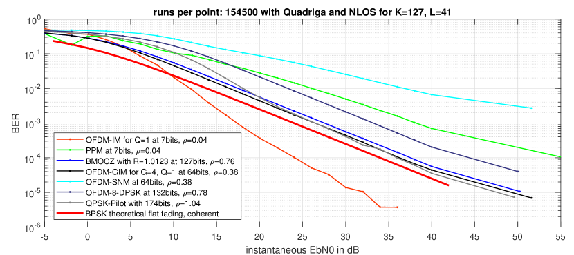
(a)

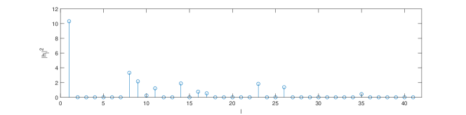
(b)

Figure 10: ((10(a))) BER of blind schemes over instantaneous SNR corrected by spectral efficiency and ((10(b))) random channel realizations with Quadriga at maximal delay spread $L=41$.

We used the version 2.0 of the Quadriga channel simulator [13], to generate random CIRs for the Berlin outdoor scenario (“BERLIN_UMa_NLOS”), with NLOS at a carrier frequency $f_{c}=4$Ghz and bandwith $W=150$Mhz, see Figure (10(a)). Transmitter and receiver are stationary using omnidirectional antennas ($\lambda/2$). The transmitter might be a base station mounted at $10$m altitude and the receiver might be a ground user with ground distance $20$m. The LOS distance is then $\approx 22$m.

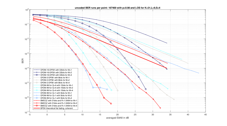
(a)

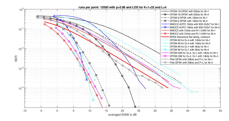
(b)

Figure 11: BMOCZ comparison to OFDM-IM, -GIM, -DPSK with $2$ OFDM symbols, and Pilot-QPSK for $1$ and $4$ antennas at maximal CIR length $L=9$ in ((11(a))) and $L=4$ in ((11(b))).

VI Conclusion

We proposed a timing-offset and carrier frequency offset estimation for the novel BMOCZ modulation scheme in wideband frequency-selective fading channels. The CFO robustness is realized by a cyclically permutable code, which allows to identify the integer CFO. An oversampled DiZeT decoder allows to estimate the fractional CFO. The CPC code construction with cyclic BCH codes allow to correct additional bit errors which enhances the performance of the BMOCZ design for moderate SNRs. Furthermore, we used a novel simulation software Quadriga version 2.0, to generate random CIR at a bandwidth of $150$Mhz. Due to the low-latency of BMOCZ the CFO and TO estimation from one single BMOCZ symbol, this blind scheme is ideal for control-channel applications, where few critical and control data need to be exchanged while at the same time, channel and impairments information need to be communicated and estimated. Coded BMOCZ with ACPC is therefore a promising scheme to enable low-latency and ultra-reliable short-packet communications over unknown wideband channels.

VII Acknowledgements

The authors would like to thank Richard Kueng, Anatoly Khina, and Urbashi Mitra for many helpful discussions. Peter Jung is supported by DFG grant JU 2795/3.

References

References

- [1] Philipp Walk, Peter Jung and Babak Hassibi “Noncoherent Short Packet Communication via Modulation on Conjugated Zeros” In Arxiv, 2018 A: 1805.07876
- [2] P. Walk, P. Jung and B. Hassibi “MOCZ for Blind Short-Packet Comunication: Basic Principles” In submitted to Trans. Wireless Commun., 2018
- [3] David Tse and Pramod Viswanath “Fundamentals of Wireless Communication” Cambridge University Press, 2005
- [4] P. H. Moose “A technique for orthogonal frequency division multiplexing frequency offset correction” In IEEE Transactions on Communications 42.10 Institute of ElectricalElectronics Engineers (IEEE), 1994, pp. 2908–2914 DOI: 10.1109/26.328961
- [5] Xiaofei Zhang, Xin Gao and Dazhuan Xu “Novel blind carrier frequency offset estimation for OFDM system with multiple antennas” In IEEE Transactions on Wireless Communications 9.3 Institute of ElectricalElectronics Engineers (IEEE), 2010, pp. 881–885 DOI: 10.1109/TWC.2010.03.081149
- [6] Jungwon Lee, Hui-Ling Lou, D. Toumpakaris and J. M. Cioffi “Effect of carrier frequency offset on OFDM systems for multipath fading channels” In IEEE Global Telecommunications Conference, 2004. GLOBECOM IEEE, 2004 DOI: 10.1109/GLOCOM.2004.1379064
- [7] H. Liu and U. Tureli “A high-efficiency carrier estimator for OFDM communications” In IEEE Communications Letters 2.4 Institute of ElectricalElectronics Engineers (IEEE), 1998, pp. 104–106 DOI: 10.1109/4234.664219
- [8] U. Tureli, H. Liu and M. D. Zoltowski “OFDM blind carrier offset estimation: ESPRIT” In IEEE Transactions on Communications 48.9 Institute of ElectricalElectronics Engineers (IEEE), 2000, pp. 1459–1461 DOI: 10.1109/26.870011
- [9] Yong Soo Cho, Jaekwon Kim, Won Young Yang and Chung G. Kang “MIMO-OFDM Wireless Communications with MATLAB®” John Wiley & Sons, Ltd, 2010 DOI: 10.1002/9780470825631
- [10] Jeongho Park, Jihyung Kim, Myonghee Park, Kyunbyoung Ko, Changeon Kang and Daesik Hong “Performance analysis of channel estimation for OFDM systems with residual timing offset” In IEEE Transactions on Wireless Communications 5.7, 2006, pp. 1622–1625 DOI: 10.1109/twc.2006.1673071
- [11] T. M. Schmidl and D. C. Cox “Robust frequency and timing synchronization for OFDM” In IEEE Transactions on Communications 45.12 Institute of ElectricalElectronics Engineers (IEEE), 1997, pp. 1613–1621 DOI: 10.1109/26.650240
- [12] T. M. Schmidl and D. C. Cox “Low-overhead, low-complexity [burst] synchronization for OFDM” In Proceedings of ICC/SUPERCOMM - International Conference on Communications IEEE, 1996 DOI: 10.1109/ICC.1996.533620
- [13] Stephan Jaeckel, Leszek Raschkowski, Kai Borner and Lars Thiele “QuaDRiGa: A 3-D Multi-Cell Channel Model With Time Evolution for Enabling Virtual Field Trials” In IEEE Transactions on Antennas and Propagation 62.6 Institute of ElectricalElectronics Engineers (IEEE), 2014, pp. 3242–3256 DOI: 10.1109/TAP.2014.2310220
- [14] Da.A. Huffman “The generation of impulse-equivalent pulse trains” In IRE Trans. Inf. Theory 8, 1962
- [15] S. S. Ghassemzadeh, L. J. Greenstein, A. Kavcic, T. Sveinsson and V. Tarokh “UWB indoor delay profile model for residential and commercial environments” In 2003 IEEE 58th Vehicular Technology Conference. VTC 2003-Fall (IEEE Cat. No.03CH37484) IEEE, 2003 DOI: 10.1109/VETECF.2003.1286198
- [16] D. Cassioli, M. Z. Win and A. F. Molisch “The ultra-wide bandwidth indoor channel: from statistical model to simulations” In IEEE Journal on Selected Areas in Communications 20.6 Institute of ElectricalElectronics Engineers (IEEE), 2002, pp. 1247–1257 DOI: 10.1109/JSAC.2002.801228
- [17] Solomon W. Golomb and Guang Gong “Signal Design for Good Correlation: For Wireless Communication, Cryptography, and Radar” Cambridge University Press, 2005
- [18] P. Walk, P. Jung and B. Hassibi “Short-Message Communication and FIR System Identification using Huffman Sequences” In IEEE International Symposium on Information Theory, 2017 DOI: 10.1109/ISIT.2017.8006672
- [19] P. Walk, P. Jung and G. E. Pfander “On the Stability of Sparse Convolutions” In Applied and Computational Harmonic Analysis 42, 2017, pp. 117–134 DOI: doi:10.1016/j.acha.2015.08.002
- [20] S. Boyd and L. Vandenberghe “Convex Optimization” Cambridge University Press, 2004
- [21] Simon Foucart and Holger Rauhut “A Mathematical Introduction to Compressive Sensing”, Applied and Numerical Harmonic Analysis Birkhäuser, 2013
- [22] S. W. Golomb “Shift Register Sequences”, 1967
- [23] G. Redinbo and J. Wolcott “Systematic Construction of Cyclically Permutable Code Words” In IEEE Transactions on Communications 23.7 Institute of ElectricalElectronics Engineers (IEEE), 1975, pp. 786–789 DOI: 10.1109/TCOM.1975.1092875
- [24] V. C. Rocha, J. S. Lemos-Neto and M. L. M. G. Alcoforado “Uniform constant composition codes derived from repeated-root cyclic codes” In Electronics Letters 54.3 Institution of EngineeringTechnology (IET), 2018, pp. 146–148 DOI: 10.1049/el.2017.2008
- [25] S. W. Golomb, Basil Gordon and L. R. Welch “Comma-free codes” In Journal canadien de mathématiques 10.0 Canadian Mathematical Society, 1958, pp. 202–209 DOI: 10.4153/CJM-1958-023-9
- [26] Vladimir I. Levenshtein “Combinatorial problems motivated by comma-free codes” In Journal of Combinatorial Designs 12.3 Wiley, 2004, pp. 184–196 DOI: 10.1002/jcd.10071
- [27] E. Gilbert “Cyclically permutable error-correcting codes” In IEEE Transactions on Information Theory 9.3 Institute of ElectricalElectronics Engineers (IEEE), 1963, pp. 175–182 DOI: 10.1109/TIT.1963.1057840
- [28] M. Kuribayashi and H. Tanaka “How to Generate Cyclically Permutable Codes From Cyclic Codes” In IEEE Transactions on Information Theory 52.10 Institute of ElectricalElectronics Engineers (IEEE), 2006, pp. 4660–4663 DOI: 10.1109/TIT.2006.881834
- [29] Akbar Sayeed and Adrian Perrig “Secure wireless communications: Secret keys through multipath” In Acoustics, Speech and Signal Processing, 2008. ICASSP 2008. IEEE International Conference on, 2008, pp. 3013–3016 IEEE
- [30] J.S. Lemos-Neto and V.C. Rocha “Cyclically permutable codes specified by roots of generator polynomial” In Electronics Letters 50.17 Institution of EngineeringTechnology (IET), 2014, pp. 1202–1204 DOI: 10.1049/el.2014.0296
- [31] Richard E. Blahut “Algebraic codes for data transmission” Cambridge University Press, 2003
- [32] Miaowen Wen, Xiang Cheng and Liuqing Yang “Index Modulation for 5G Wireless Communications” Springer, 2017 DOI: 10.1007/978-3-319-51355-3
- [33] Victor Monzon Baeza, Ana Garcia Armada, Mohammed El-Hajjar and Lajos Hanzo “Performance of a Non-Coherent Massive SIMO M-DPSK System” In 2017 IEEE 86th Vehicular Technology Conference (VTC-Fall) IEEE, 2017 DOI: 10.1109/VTCFall.2017.8288015
- [34] H. Jafarkhani “Space-Time Coding: Theory and Practice” Cambridge, 2005