Modeling Heterogeneity in Mode-Switching Behavior
Under a Mobility-on-Demand Transit System:
An Interpretable Machine Learning Approach

Abstract

Over the last decade, machine learning has been applied to many engineering and scientific disciplines, often achieving high predictive accuracy. Recent years, however, have witnessed an increased focus on interpretability and the use of machine learning to inform policy analysis and decision making. This paper applies machine learning to examine travel behavior and, in particular, on modeling changes in travel modes when individuals are presented with a novel (on-demand) mobility option. It addresses the following question: Can machine learning be applied to model individual taste heterogeneity (preference heterogeneity for travel modes and response heterogeneity to travel attributes) in travel mode choice?

This paper first develops a high-accuracy classifier to predict mode-switching behavior under a hypothetical Mobility-on-Demand Transit system (i.e., stated-preference data), which represents the case study underlying this research. We show that this classifier naturally captures individual heterogeneity available in the data. Moreover, the paper derives insights on heterogeneous switching behaviors through the generation of marginal effects and elasticities by current travel mode, partial dependence plots, individual conditional expectation plots. The paper also proposes two new model-agnostic interpretation tools for machine learning, i.e., conditional partial dependence plots and conditional individual partial dependence plots, specifically designed to examine response heterogeneity. The results on the case study show that the machine-learning classifier, together with model-agnostic interpretation tools, provides valuable insights on travel mode switching behavior for different individuals and population segments. For example, the existing drivers are more sensitive to additional pickups than people using other travel modes, and current transit users are generally willing to share rides but reluctant to take any additional transfers. These insights can be used to inform transportation planning and the design of new mobility services.

1 Introduction

The popularity of machine learning is continuously increasing in transportation, with applications ranging from traffic engineering to travel demand forecasting and pavement material modeling, to name just a few. In general, machine learning achieves greater predictive accuracy compared to traditional methods. However, there is also a recognition in the field that a single metric, such as the predictive accuracy or mean squared error, provides an incomplete description of the complexities arising in the real world [10]. As a result, in many disciplines, increased attention is being devoted to the interpretability of machine-learning results.

This paper applies machine learning to model travel behavior and, in particular, to model the switching from traveler’s usual commute travel modes to a novel Mobility-on-Demand (MOD) option. Previous studies have applied Machine learning to model travel behavior [e.g., 40, 34, 14, 43]. These studies often find that machine learning can predict individual travel-mode choice more accurately than traditional random utility models, the de facto standard in travel-behavior modeling. Nonetheless, previous work rarely discuss how to interpret machine-learning models and derive behavioral insights from the model outputs in order to inform transportation planning and policymaking. These are areas where random utility models typically excel due to their microeconomic foundations and the natural interpretations of the utility functions.

This paper extends the applications of machine-learning methods in travel-mode modeling from a mere focus on prediction to detailed behavioral interpretations. Its primary goal is to derive behavioral insights from machine-learning methods that can then be used to inform transportation planning and policy intervention. More specifically, the paper examines individual taste heterogeneity, an essential research topic in travel behavior modeling that has been a primary focus within the random utility framework [e.g., 33, 36, 4, 20, 5]. To our knowledge, the application of interpretable machine learning to model heterogeneity in travel behavior is novel and is largely absent from the existing literature.

This paper provides a case study of applying machine learning to model heterogeneity in mode switching behavior, in the context of a proposed MOD Transit system that integrates fixed-route services and on-demand shuttles [23]. It first derives a high-fidelity predictive model based on machine learning. The paper then shows that the best-performing machine-learning model (Boosting trees [BOOST]) can naturally segment the entire population and capture heterogeneous mode-switching behavior. Specifically, the paper demonstrates that behavioral insights can be revealed through the generation of marginal effects and elasticities for different market segments, partial dependence plots (PDPs), and individual conditional expectation (ICE) plots. Moreover, the paper proposes two new concepts, conditional partial dependence plots (CPDPs) and conditional individual partial dependence plots (CIPDPs), which allows machine learning to capture taste heterogeneity between and across different market segments. As the results of the case study suggest, these novel tools can generate valuable insights regarding the potential adoption of the MOD Transit system and the impact of the underlying design decisions.

The rest of the paper is organized as follows. Section 2 summarizes the research background and includes three major parts, i.e., machine-learning applications in travel behavior modeling, modeling heterogeneity in travel behavior, and interpretable machine learning. Section 3 describes the methodological framework underlying this paper: It discusses the use of machine learning for travel choice modeling and available tools for interpreting the heterogeneous mode switching behavior. In addition, it presents two novel tools, CPDPs and CIPDPs, which allow for the generation of more behavioral insights by applying market segmentation. Section 4 describes a case study, which includes the data description, the specification of machine-learning classifiers, and the training, validation, and testing procedure. Section 5 presents results on the predictive capability of machine learning, PDPs and CPDPs, ICE plots and CIPDPs, and marginal effects and elasticities for different market segments. Finally, Section 6 summarizes the findings, identifies the benefits and limitations of the proposed approach, and suggests future research directions.

2 Research Background

2.1 Machine Learning Applications in Travel Behavior Modeling

In recent years, researchers started to apply machine-learning methods to model individual travel behavior [e.g., 40, 34, 14, 39]. For example, Xie et al. [40] applied decision trees and neural networks (NN) to model individual mode choice and showed that these two models could improve the predictive accuracy of the multinomial logit model. Later, Tang et al. [34] also applied decision trees to model travel mode switching behavior and obtained higher accuracy than logit models in most cases. More recently, Hagenauer and Helbich [14] provided a comparison of various machine-learning classifiers for modeling travel mode choice, focusing primarily on predictive accuracy. Wang and Ross [39] found that the extreme gradient boosting model substantially exceeded the prediction performance of the multinomial logit model when modeling travel mode choices.

Even though machine learning has demonstrated its strength in mode-choice predictions, there has been little discussion regarding interpreting the machine learning model outputs to extract behavioral insights. That is to say, knowledge on the underlying decision rules that machine learning uses for travel-behavior prediction is lacking. Zhao et al. [43] provides an early probe into this issue. They conducted a comprehensive comparison between machine learning and random utility models and found that that machine learning can not only offer a more flexible modeling structure and achieve higher predictive accuracy than traditional logit models, but also produce comparable behavioral outputs such as marginal effects and elasticities.

2.2 Modeling taste Heterogeneity in Travel Behavior

Travel behavior heterogeneity has been extensively studied within the random utility modeling framework. There are two types of taste heterogeneity: one is preference heterogeneity, which refers to the varying levels of preference for different travel modes across individuals; the other is response heterogeneity, which indicates travelers’ varying levels of sensitivity to changes in travel attributes. From a modeler’s perspective, taste heterogeneity can be divided into two parts, i.e., observed and unobserved. Observed heterogeneity can be captured by introducing observed individual socio-demographic or behavioral characteristics as alternative specific variables and/or by capturing interactions between level-of-service variables and observed individual features, e.g., by applying a market segmentation approach or adding interaction terms [4]. The market segmentation approach means to select subgroups from a population in advance based on the known characteristics and declare them as “segments,” aiming at analyzing a manageable number of groups that share well-defined underlying features and generating more creative and better-targeted policies for different groups [1]. On the other hand, unobserved heterogeneity is usually caused by unobserved individual features, such as individuals’ intrinsic bias towards different travel modes or their varying degrees of sensitivity to level-of-service attributes [4]. To account for unobserved heterogeneity, researchers usually applied mixed logit models to fit random coefficients for explanation variables and/or to fit flexible error terms (the independent Gumbel distributed part plus the correlated normal distributed part) to account for the correlations over alternatives [20].

With strong theoretical foundations, random utility models have been widely applied to model heterogeneity [e.g., 33, 36, 4, 20, 5]. For instance, Bhat [4] took into account observed and unobserved heterogeneity for modeling urban work travel mode choice. Srinivasan and Mahmassani [33] proposed a dynamic kernel logit formulation to analyze heterogeneity and unobserved structural effects in route-switching behavior. To capture the disaggregate decision-making more accurately, researchers have used the integrated choice and latent variable models in assessing heterogeneous travel behavior [36].

Nevertheless, since random utility models often have low prediction performance [14, 43], one may think that the behavioral insights generated from them are less trustworthy than those based on models with higher predictive accuracy. Moreover, recent studies have suggested that, unlike conventional random utility models that require extensive modeling effort and domain knowledge to accommodate individual heterogeneity, machine learning models can account for it automatically. For example, Lhéritier et al. [19] compared the random forest (RF) model with the latent class multinomial logit model through a series of experiments, and found that the RF model has the ability of segmenting population groups (with heterogeneous tastes) automatically. Therefore, it would be worthwhile to study the application of interpretable machine learning techniques to examine individual taste heterogeneity.

2.3 Interpretable Machine Learning

Interpretable machine learning is receiving increasing attention in recent years [e.g. 27, 11, 10, 26, 42, 37, 3]. In particular, Murdoch et al. [27] defined interpretable machine learning as applying machine-learning methods to extract relevant knowledge about the domain relationships contained in the data.

The methods for machine-learning interpretability may be divided into two categories, i.e., intrinsic and post hoc. As discussed in Molnar [26], intrinsic interpretability usually refers to relatively simple machine-learning models that are considered interpretable due to their simple model structure, such as linear regression, logit models, and decision trees. On the other hand, post hoc interpretability of a machine-learning model is achieved by applying interpretation methods after its training and application. The machine-learning interpretation methods can also be divided into model-specific or model-agnostic. Model-specific methods can only be applied to a specific class of models, while model-agnostic methods can be applied to any machine-learning models after training. Since model-agnostic interpretation methods have lots of flexibility compared to their dedicated counterparts and can provide consistent interpretability criteria for any model class, this paper focuses on applying and inventing model-agnostic interpretation methods to explain individual travel behavior.

One of the most prevalent model-agnostic methods is the PDP, which presents the dependence between the response variable and a set of input features, marginalizing over the values of the remaining features [12]. As an extension of PDP, Goldstein et al. [13] proposed another model-agnostic method—the ICE plots—to reveal the potential individual heterogeneity by generating one curve per observation that presents how its prediction evolves when a feature changes. Notably, PDPs and ICE plots were recently proved to be effective to reveal causal inference between input features and the response variable [42]. In addition, Wager and Athey [37] assessed estimation and inference of heterogeneous treatment effects using RF. However, PDPs and ICE curves focus on all the instances under evaluation without looking at the specific groups of people to gain additional insights on taste heterogeneity across different population groups. Therefore, this paper introduces two new model-agnostic methods as an extension of PDP and ICE plots, in order to better uncover the taste heterogeneity within and across different population segments.

Some model-agnostic methods have been applied in some of the existing literature of travel behavior modeling, such as Hagenauer and Helbich [14], Wang and Ross [39]. However, their discussion mainly focused on variable importance (measures the importance of a feature for prediction). Our prior work [43] showcased how to apply PDPs to evaluate the marginal impacts of the selected features. However, to our knowledge, no existing work focuses on applying existing machine-learning interpretation tools or developing new ones to reveal heterogeneous travel behavior for informing the design of MOD Transit and policy analysis.

3 Methodological Framework

This paper is interested in the following research question: What factors and how they shape individual willingness to switch to a new transportation mode? The paper approaches this question using the following methodological framework. It assumes the availability of a longitudinal dataset that captures individual travel mode choice before and after a new mobility option is introduced. If the new mobility service is not yet deployed, a stated-preference (SP) survey can be conducted to capture individual preferences for the new travel mode. The data can be represented as $\{\boldsymbol{x}_{i},y_{i}\}_{i=1}^{N}$, where $\boldsymbol{x}_{i}=[x_{i1},...,x_{ip}]$ is a vector of $p$ features for individual $i$ and $y_{i}$ is the response variable. The features $\boldsymbol{x}_{i}$ often include socio-economic and demographic information, travel preference, current travel mode, and the level-of-service variables for each travel mode under evaluation. The response variable $y_{i}$ is binary: Value 0 indicates that individual $i$ stays with her current mode and value 1 indicates that individual $i$ switches to the new travel mode.

3.1 Choice Modeling with Machine Learning

Choice modeling with machine learning is typically approached as a classification problem [40, 14, 43]. Commonly used classification models include logistic regression (logit) [15], Support Vector Machines (SVM) [9], RF [7], and BOOST [12]. The classification approaches can be divided into two categories, i.e., soft and hard classification [38, 22]. Soft classification estimates the class conditional probabilities first and then predicts the class based on the largest estimated probability [22]. On the other hand, hard classification predicts the class labels directly without estimating intermediate class probabilities. Most prior work in machine learning for choice modeling are based on hard classification [e.g. 40, 34, 39]. However, it is more natural to use class probabilities (estimated by soft classification) to predict market shares, especially when the sample size is small. For example, if the sample population contains a hundred people for which the predicted switching probabilities are all 0.51, a hard classification will predict switching in 100% of the cases, while a soft classification would concludes that switching occurs in 51% of the cases.

This paper treats the prediction of travel mode switching as a soft classification problem. The classifier $f(\boldsymbol{x}|\hat{\boldsymbol{\theta}})$ (where $\hat{\boldsymbol{\theta}}$ is an estimated parameter or hyperparameter vector) maps the features $\boldsymbol{x}$ to the response variable $\boldsymbol{y}$ using the predictions of class probabilities, i.e.,

$$\hat{y}_{i}=\operatorname*{arg\,max}_{k\in\{0,1\}}\hat{p}_{i,k}$$ (1)

where $\hat{p}_{i,k}$ is the predicted choice probability for class $k$ ($k\in\{0,1\}$) of observation $i$ ($i=1,2,...,N$).

The predictive accuracy at the individual level of different classifiers is evaluated using the formula

$$\sum_{i=1}^{N}I_{y_{i}}(\hat{y}_{i})/N,$$ (2)

where $I_{y_{i}}(\hat{y}_{i})$ is an indicator function which equals to 1 when $\hat{y}_{i}=y_{i}$.

The predicted market share for class $k$ is computed using the formula

$$Q_{k}(\boldsymbol{x}|\hat{\boldsymbol{\theta}})=\frac{1}{N}\sum_{i=1}^{N}\hat{p}_{ik}$$ (3)

that averages the predicted choice probabilities for all the instances. The predictive accuracy at the aggregate level is evaluated using the L1-Norm, i.e.,

$$\sum_{k=0}^{1}\Big{|}Q_{k}^{*}-Q_{k}(\boldsymbol{x}|\hat{\boldsymbol{\theta}})\Big{|},$$ (4)

where $Q_{k}^{*}$ represents the observed market share for choice $k\in\{0,1\}$.

The training, validation, and testing of the classifiers, as well as the model selection, are discussed in detail in Subsection 4.3.

3.2 Interpreting Heterogeneous Mode Switching Behavior

Soft classification helps the interpretation of heterogeneous switching behavior. This section reviews some existing interpretation techniques, including PDPs and their extensions in ICE curves. In addition, it proposes two new tools for interpretation, CPDPs and CIPDPs. Finally, this section reports marginal effects and elasticities for market segments in order to further understand individual taste heterogeneity.

3.2.1 Partial Dependence Plots (PDPs) and Individual Conditional Expectation (ICE) Plots

PDPs, first proposed by Friedman [12], are one of the most popular model-agnostic interpretation tools for machine-learning models. Assume that we are interested in determining the effect of a set $S\subset\{1,...,p\}$ of features on the prediction outcomes and let $C$ be the complement of $S$ (i.e., $C=\{1,...,p\}\setminus S$). The partial dependence of classifier $f$ on $\boldsymbol{x}_{S}$ is defined as

$$f_{S}(\boldsymbol{x}_{S})=\mathbb{E}_{\boldsymbol{x}_{C}}f(\boldsymbol{x}_{S},\boldsymbol{x}_{C}|\boldsymbol{\theta}).$$ (5)

In practice, Eqn. (5) is estimated by computing

$$\hat{f}_{S}(\boldsymbol{x}_{S})=\frac{1}{N}\sum_{i=1}^{N}f(\boldsymbol{x}_{S},\boldsymbol{x}_{C_{i}}|\hat{\boldsymbol{\theta}}),$$ (6)

where $\boldsymbol{x}_{C_{i}}(i=1,...,N)$ represent the values of $\boldsymbol{x}_{C}$ for each instance in the training set. The PDP evaluates the influence of $\boldsymbol{x}_{S}$ on $\hat{f}$ after marginalizing over all the other features. For soft classifiers, the PDP displays the class probability (e.g., the switching probability) for each possible value of $\boldsymbol{x}_{S}$. As discussed in Friedman [12], the PDP can be a useful summary of the impact of the chosen subset of features when the interactions between the chosen features and the remaining features are weak. However, when the interactions are strong, the PDPs may obscure a heterogeneous relationship created by the interactions [13].

To complement PDPs, Goldstein et al. [13] proposed ICE plots to capture the potential individual heterogeneity. Instead of plotting the average partial dependence on the predicted response, the ICE curve generates an estimated conditional expectation curve

$$\hat{f}_{S}^{i}(\boldsymbol{x}_{S})=f(\boldsymbol{x}_{S},\boldsymbol{x}_{C_{i}}|\hat{\boldsymbol{\theta}}),$$ (7)

for each instance $C_{i}$ $(i=1,\ldots,N)$ in the dataset. The average of all the ICE plots is the corresponding PDP for the selected feature [26]. As ICE plots generate individual-specific curves, it can be used directly to understand taste heterogeneity.

PDPs and ICE plots are easy to implement and provide clear interpretations of a classifier. In particular, ICE plots are capable of revealing individual heterogeneity (by producing individual-specific curves), which is an important topic in travel behavior modeling. Furthermore, as discussed by Zhao and Hastie [42], PDPs and ICE plots may reveal causal relationships if $f$ is an accurate classifier and domain knowledge supports the underlying causal structure.

It is important to point out that PDPs can be thought as a counterpart in machine learning relative to the beta coefficients in a logit model. A PDP graphically illustrates the relationship between an input feature and the response variable. For linear machine-learning models, the PDP would be a straight line, whose slope is equivalent to a beta coefficient; for nonlinear models, the PDP would be a curvy line with different beta coefficients (i.e. tangent of the line) at different data points. To compare the results of PDP from nonlinear machine-learning models with the beta coefficient in a logit model, we propose to use a straight line to approximate the relationship displayed in the PDP by calculating a single slope for the PDP using:

$$\frac{\hat{p}_{1}^{\text{max}}-\hat{p}_{1}^{\text{min}}}{x_{\text{max}}-x_{\text{min}}}$$ (8)

where $x_{\text{max}}$ and $x_{\text{min}}$ are the maximum and minimum values of a selected feature, and $\hat{p}_{1}^{\text{max}}$ and $\hat{p}_{1}^{\text{min}}$ are the corresponding estimated switching probabilities at $x_{\text{max}}$ and $x_{\text{min}}$ respectively. Note that the beta coefficients of a logit model are in the logit region (or log-odds region), while the the slopes of PDPs are in the probability domain.

3.2.2 Conditional Partial Dependence Plots (CPDPs) and Conditional Individual Partial Dependence Plots (CIPDPs)

This paper also proposes two new model-agnostic tools for improving the interpretations of classifiers and revealing additional insights in presence of individual heterogeneity: CPDPs and CIPDPs. The key idea behind CPDPs and CIPDPs is to group instances into subpopulations based on some observed features (i.e., a market segmentation approach). These plots further allow researchers to examine response heterogeneity across different population groups.

This paper uses the observed socio-demographic or behavioral features to segment the market in order to examine observed heterogeneity. For example, the instances can be grouped by income, gender, or current commuting mode. By plotting the ICE curves within each market segment and computing the corresponding PDP for the subpopulation, it is possible to contrast the behaviors of different population groups and different individuals within these groups.

More formally, consider a categorical feature $g$ and its set $V$ of possible values. A CPDP conditioned on feature $g$ is defined as

$$f_{S}(\boldsymbol{x}_{S})_{\mid x_{g}=v}=\mathbb{E}_{\boldsymbol{x}_{C}}f(\boldsymbol{x}_{S},\boldsymbol{x}_{C}|\boldsymbol{\theta},x_{g}=v)$$ (9)

for each value $v\in V$. This definition can be generalized to a set $\boldsymbol{G}$ of features

$$f_{S}(\boldsymbol{x}_{S})_{\mid\boldsymbol{x}_{\boldsymbol{g}}=\boldsymbol{v}}=\mathbb{E}_{\boldsymbol{x}_{C}}f(\boldsymbol{x}_{S},\boldsymbol{x}_{C}|\boldsymbol{\theta},\boldsymbol{x}_{\boldsymbol{g}}=\boldsymbol{v}).$$ (10)

CIPDPs are the conditional counterpart to the ICE curves. Given a feature $g$ and a value $v$ of interest, CIPDPs will display the ICE curves, $f_{S}^{j}(\boldsymbol{x}_{S})$, for those instances $j$ satisfying $x_{g,j}=v$, $j\in\{1,...,N\}$. These definitions can be naturally extended to non-categorical attributes by partitioning their domains.

Compared to PDPs and ICE plots, CIPDPs and CPDPs mainly assess the pre-determined mutually-exclusive subgroups of the training set. By segmenting the market based on the prior knowledge of the travel behavior theory, CIPDPs and CPDPs are expected to be useful to capture diverse behaviors across and within different population groups.

3.2.3 Marginal Effects and Elasticities for Market Segments

Marginal effects and elasticities are widely-used econometric concepts to indicate the sensitivity of an outcome variable with respect to changes in independent variables. In mode-choice applications, they are defined as the changes in the choice probability of an alternative in response to a one unit (percent) change in an independent variable. These tools can be applied to machine-learning classifiers too, as shown in Zhao et al. [43]. The marginal effects and arc elasticities of feature $\boldsymbol{x}_{t},t=1,...,p$, for class $k$ can be computed as:

$$M_{k}(\boldsymbol{x}_{t})=\frac{Q_{k}(\boldsymbol{x}_{-t},\boldsymbol{x}_{t}+\delta|\hat{\boldsymbol{\theta}})-Q_{k}(\boldsymbol{x}|\hat{\boldsymbol{\theta}})}{|\delta|},$$ (11)

$$E_{k}(\boldsymbol{x}_{t})=\frac{[Q_{k}(\boldsymbol{x}_{-t},\boldsymbol{x}_{t}\cdot(1+\delta)|\hat{\boldsymbol{\theta}})-Q_{k}(\boldsymbol{x}|\hat{\boldsymbol{\theta}})]/Q_{k}(\boldsymbol{x}|\hat{\boldsymbol{\theta}})}{|\delta|},$$ (12)

where $\boldsymbol{x}_{-t}\in\mathbb{R}^{p-1}$ represents the complement set of $\boldsymbol{x}_{t}$ and $\delta$ is a constant.

In order to uncover heterogeneity across different population groups, one can also compute marginal effects and elasticities for different market segments instead of for the entire population. For instance, for a categorical feature $g$ and its potential value $v$, the marginal effects and elasticities can be defined as

$$M_{k}(\boldsymbol{x}_{t})_{|x_{g}=v}=\frac{Q_{k}(\boldsymbol{x}_{-{t}},\boldsymbol{x}_{t}+\delta|\hat{\boldsymbol{\theta}},x_{g}=v)-Q_{k}(\boldsymbol{x}|\hat{\boldsymbol{\theta}},x_{g}=v)}{|\delta|},$$ (13)

$$E_{k}(\boldsymbol{x}_{t})_{|x_{g}=v}=\frac{[Q_{k}(\boldsymbol{x}_{-{t}},\boldsymbol{x}_{t}\cdot(1+\delta)|\hat{\boldsymbol{\theta}},x_{g}=v)-Q_{k}(\boldsymbol{x}|\hat{\boldsymbol{\theta}},x_{g}=v)]/Q_{k}(\boldsymbol{x}|\hat{\boldsymbol{\theta}},x_{g}=v)}{|\delta|}.$$ (14)

As discussed by Zhao et al. [43], some machine-learning classifiers, such as tree-based models, split input feature values at different nodes. Therefore, the prediction decisions for these models become insensitive to changes in feature value outside its range. As a result, this paper only predicts the marginal effects and elasticities for instances within the data range. Subsection 5.4 provides more details on this topic.

4 Case Study

4.1 The Data

The case study uses data collected from a SP survey by faculty, staff, and students at the University of Michigan, Ann Arbor. The survey first asked the participants to estimate the travel time, cost, and wait time for their commuting trip from one of the following modes: Car, Walk, Bike, and Bus. Then, by showing them a new MOD Transit system that would replace the existing transit system, the survey asked them what travel mode (i.e., Car, Walk, Bike, and MOD Transit) they might choose in a different state-choice experiments (with different levels of service for MOD Transit). The detailed survey description with graphical illustrations can be found in Yan et al. [41].

This paper aims at evaluating the factors underlying individuals’ intention to switch to the new MOD Transit system. That is to say, some travel behavior changes, such as switching from Car to Bike, is not of interest in this study. Hence, the outcomes of the state-choice experiments are expressed as binary answers, where value 0 represents the decision of not switching to MOD Transit and 1 denotes the decision of switching to MOD Transit. MOD Transit is considered as a new travel mode here, that is to say, individuals who currently use the bus are considered as switch to MOD Transit if he or she select the new mode.

Table 1: Statistics for Features and Response Variable.

Variable	Description	Category	%	Min	Max	Mean	SD
Response Variable
Switching Choice		MOD Transit	35.28
		Not MOD Transit	64.72
Features
TT_Drive	Travel time of driving (min)			2.00	40.00	15.21	6.62
TT_Walk	Travel time of walking (min)			3.00	120.00	32.30	23.08
TT_Bike	Travel time of biking (min)			1.00	55.00	15.34	10.45
TT_MOD	Travel time of using MOD transit (min)			6.20	34.00	18.68	4.75
Wait_Time	Wait time for MOD (min)			3.00	8.00	5.00	2.07
Transfer	Number of transfers in MOD			0.00	2.00	0.33	0.65
Rideshare	Number of additional pickups in MOD			0.00	2.00	1.11	0.82
Income	Income level			1.00	6.00	1.93	1.34
Bike_Walkability	Importance of bike- and walk-ability			1.00	4.00	3.22	0.95
MOD_Access	ease of access to MOD			1.00	4.00	3.09	1.02
CarPerCap	Car per capita			0.00	3.00	0.53	0.48
Female	Female or Male	Female	56.32
		Male	43.68
Student	Students or faculty/staff	Student	73.52
		Faculty or staff	26.48
Current_Mode_Car	Current travel mode is Car or not	Car	16.68
		Not Car	83.32
Current_Mode_Walk	Current travel mode is Walk or not	Walk	40.41
		Not Walk	59.59
Current_Mode_Bike	Current travel mode is Bike or not	Bike	8.25
		Not Bike	91.75

There were 8,141 data points collected from 1,163 individuals. The statistics for 16 features and the response variable are given in Table 1. The feature “Current_Mode_Bus” (indicates whether the current travel mode is Bus) is not included for analysis, since this feature is completely correlated with the other three features: “Current_Mode_Car,” “Current_Mode_Walk,” and “Current_Mode_Bike,” with the sum of the four features equal to 1. All the variables have the variance inflation factor less than 5 (a threshold commonly referenced), which suggests that multicollinearity is not a concern.

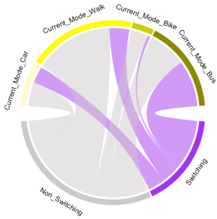
Figure 1: Chord Diagram of Switching Choice Versus Current Travel Mode Choice.

Based on the observed socio-demographic and behavioral characteristics, there are different ways to segment the market to study individual heterogeneity. Some possible market segmentation approaches include grouping people by different income levels, car ownership, gender, or commonly-used commuting modes. In particular, our previous study [43] has found out that, for the multinomial logit model, the dummy variables of the current travel modes are positive for all the four modes and statistically significant for Car, Walk, and Bike. These results indicate that travelers may present an inertia to their current modes. Moreover, as an exploratory analysis, Figure 1 presents a chord diagram illustrating graphically the inter-relationships between switching decisions and current travel modes. It is obvious that different market segments show different ratios of switching. Therefore, as an illustration, this paper chooses to segment the market using the current travel mode and shows how to apply interpretable machine learning to reveal individual heterogeneity in mode-switching behavior under a proposed MOD Transit system.

4.2 Machine-Learning Classifiers

Seven soft machine-learning classifiers are selected for comparison: They include logit, naive Bayes (NB), classification and regression trees (CART), bagging trees (BAG), BOOST, RF, and NN. This subsection briefly summarizes these classifiers: It may be skipped by those familiar with these techniques.

The logit model is arguably the most popular classifier to predict a binary outcome (i.e., switching or not switching) [15]. The logit model assumes a linear relationship between the log-odds and input features, facilitating the interpretation of the results and the derivation of policy interventions. However, the linear nature of this classifier may not reflect the true relationship between the log-odds and input features, and the logit model may exhibit a relatively low predictive accuracy.

The NB model is also widely-used for classification. It assumes that all features are independent [24]. NB is easy to construct and is often used as a baseline classifier. However, its assumption is often violated in practice, making it sensitive to highly correlated features.

The CART model builds a classification tree, where each internal node partitions the data based on the value of a selected feature and leaves capture a class decision (e.g., switching or not switching in the case study) [8]. The decision tree is susceptible to overfitting [29] and pruning techniques can control its complexity. In this study, the trees are grown without pruning, since they are very simple, i.e., less than 5-6 leaves in most cases.

Breiman [6] and Hastie et al. [15] proposed a number of tree-based ensemble methods to overcome the limitations of CART classifiers by providing more accurate, stable, and robust models. There are three major ensemble models, including BOOST, BAG, and RF. Specifically, for classification problems, BOOST models create a sequence of decision trees and each successive tree is designed to improve the predictive accuracy of its predecessor. The final prediction of the BOOST model is the weighted voting among all trees. Compared to CART, the BOOST model usually produces a higher predictive accuracy. This study applies gradient boosting [12]. 500 trees are used, with shrinkage parameter set to 0.062 and interaction depth to 45. The minimum number of observations in leaves is 10. On the other hand, BAG and RF train a set of trees using bootstrapping (i.e., sampling with replacement) [6, 17]. The only difference between BAG and RF is that BAG uses all features to train the trees while RF only selects a random subset of all the features to train the trees. For a classification problem, multiples decision trees are trained, and the majority voting among all the trees is the prediction outcome. By using bootstrapping, the BAG model can reduce the variance and overfitting problems of a single decision tree. However, by assuming variable independence, BAG cannot reduce the variance for correlated features. By contrast, RF may overcome this limitation and reduce the variance between correlated trees. For the BAG model, 500 classification trees are trained, with each tree grown without pruning. For the RF model, 600 trees are used and 14 randomly selected variables are considered for each split at internal nodes.

A basic NN model with three layers of nodes (each node is binary) was also considered. NN has an input layer, a hidden layer, and an output layer. Each node connection between adjacent layers has a weight. The hidden layer of the NN model can help measure nonlinear relationships between features and the response variable. However, NN is also susceptible to overfitting. In the paper, a NN model with a single hidden layer of 14 units is used. The connection weights are trained by back propagation with a weight decay constant of 0.1.

All the modeling and analyses are conducted in R, using following packages: stats [30], e1071 [25], tree [32], gbm [31], randomForest [21], and nnet [35].

4.3 Training, Validation, and Testing for the Classifiers

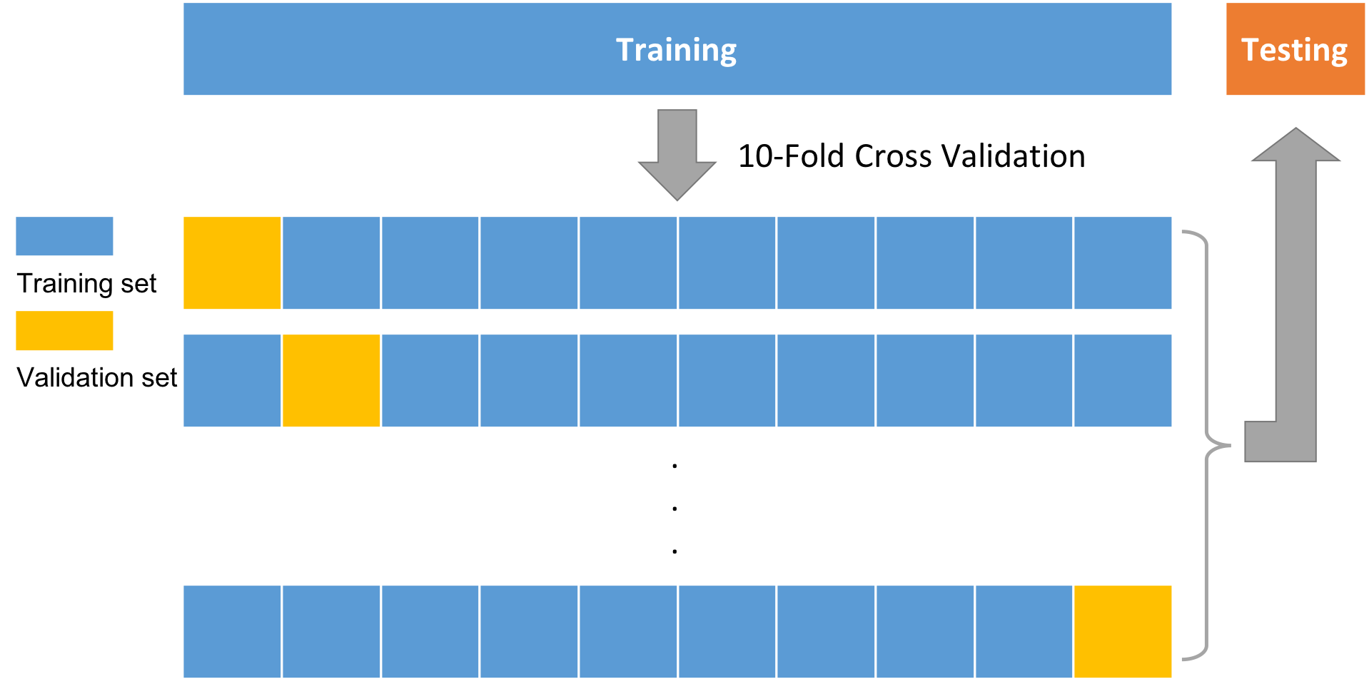
Figure 2: The Training, Validation, and Testing of the Classifiers.

To identify the best-performing model, this study trained, validated, and tested the seven machine learning classifiers using the procedure illustrated in Figure 2. First, 10% of the data is randomly drawn for the testing set using stratified sampling based on the current mode choices. In other words, the entire data set is divided into four mutually-exclusive subpopulations based on their current mode choices, i.e., Car, Walk, Bike, and Bus. Within each subpopulation, 10% samples are randomly drawn for testing.

Next, the remaining 90% of the data is used to train the model and tune hyperparameters using a 10-fold cross validation. To conduct the 10-fold cross validation, the training set is first randomly split into 10 disjoint subsets. Then, one subset is held out for validation while the remaining nine subsets are used for training the machine learning classifiers. After repeating the same process for each one of the 10 subsets, the validation outcomes for each classifier are average to obtain a mean estimate of the performance metric (e.g., the predictive accuracy). The model with the best performance metric is selected and is fitted on the entire training set (i.e., 90% of the entire data set). Finally, the selected model is applied to the testing set to provide an unbiased evaluation of its predictive capability.

5 Model Interpretation

5.1 Predictive Accuracy

The cross-validation results of seven machine learning classifiers are shown in Figure 3. With respect to the mean predictive accuracy (red lines in Figure 3), BOOST has the best outcome (0.871), followed by RF (0.860) and BAG (0.859). By contrast, the mean accuracy of the logit model is only 0.750. The model with the worst performance is CART (0.677).

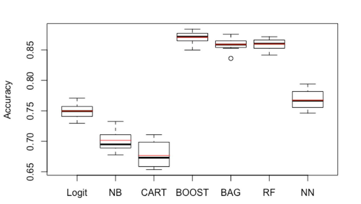
Figure 3: Accuracy of the Classifiers: Boxplots of Cross-Validation Results (Red Lines are Mean Values).

Mode/Outcome		Accuracy	L1-Norm
Overall		0.893	0.02695
Switching		0.808
Non-switching		0.939
Car	Overall	0.869	0.00213
	Switching	0.836
	Non-switching	0.890
Walk	Overall	0.904	0.04375
	Switching	0.620
	Non-switching	0.981
Bike	Overall	0.946	0.00433
	Switching	0.714
	Non-switching	0.979
Bus	Overall	0.882	0.02525
	Switching	0.890
	Non-switching	0.873

Table 2: Predicted Accuracy for all Intances and for Instances Segmented by Current Mode Choice in the Testing Set.

The BOOST model is thus selected and fitted on the entire training set. Then, the BOOST model is evaluated on the testing set and the results are presented in Table 2. The results show that the overall accuracy at the individual level is 0.893 with an accuracy of 0.808 for switching and 0.934 for non-switching predictions. By using soft classification to predict market shares, the overall L1-Norm is 0.02695, indicating that the least absolute deviation of the market share prediction is less than 3%.

Table 2 also reports the predictive capabilities of the BOOST model for different market segments (segmented by current travel mode). The testing set is divided into four mutually-exclusive subsets obtained using the current travel mode. For the overall accuracy and for the true negative rate, i.e., the rate of successfully predicting the “non-switching outcome,” the results show that BOOST performs better for individuals who currently use Car, Walk, and Bike; on the other hand, BOOST performs better in successfully predicting the “switching” outcome (i.e., true positive rate) for individuals who currently use Bus. Moreover, the prediction accuracy is more balanced (i.e., true positive rate and true negative rate are similar) for individuals using Car and Bus than individuals using Walk and Bike. One possible explanation for the relatively lower performance in predicting the switching behavior of those who currently walk or bike is the low mode-switching rates of these individuals in the training set (Walk: 20.26%; Bike: 13.45%), which resulted in an imbalanced classification problem. Properly handling the imbalanced classes in machine learning is a crucial research topic, and is an important topic for future work.

5.2 Partial Dependence Plots (PDPs) and Conditional Partial Dependence Plots (CPDPs)

The PDPs and CPDPs of the level-of-service variables (i.e., TT_MOD, Wait_Time, Transfer, and Rideshare) for MOD Transit are presented in Figure 4. The $y$-axis is the probability of switching to MOD Transit, while the $x$-axis is a level-of-service variable for the proposed system. The blue lines in Figure 4 are the PDPs, while the remaining lines are CPDPs for different market segments (Car: red; Walk: purple; Bike: pink; and Bus: yellow).

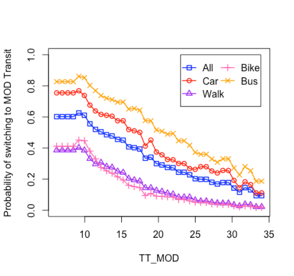
(a) Partial Dependence on TT_MOD

(b) Partial Dependence on Wait_Time

(c) Partial Dependence on Transfer

(d) Partial Dependence on Rideshare

Figure 4: PDPs and CPDPs of Level-Of-Service Variables for MOD Transit.

The PDPs have the expected decreasing trend for all the level-of-service variables: As the level-of-service for MOD Transit gets worse, the preference for MOD Transit declines for the entire market and for each market segment.

For TT_MOD (see Figure 4(a)), the corresponding PDPs and CPDPs present strong nonlinearities for the entire market and the four market segments. The probability of switching remains largely unchanged when the transit time is less than 10 minutes. For Walk and Bike, the switching probability decreases faster from 10 minutes to 20 minutes compared to that from 20 minutes to 34 minutes. For Car and Bus, the switching probability present an approximately linear decrease after 10 minutes. These results show that the MOD Transit system is highly desirable across different market segments when the transit time is relatively small (i.e., less than 10 minutes). In addition, there exists some non-smooth perturbations in the PDPs and CPDPs, even though the general trend is decreasing. This is probably caused by the tree structure of the BOOST model. For Wait_Time and Transfer, some nonlinearities are also present as illustrated in Figure 4(b)-4(c). To be specific, for all the subpopulations, the switching probability has larger decrease for Wait_Time from 3 minutes to 5 minutes than that from 5 minutes to 8 minutes. In addition, within the analysis range for Transfer (i.e., 0–2), the probability of switching to MOD Transit has larger decline for the second transfer than the first transfer. One insight is that one may consider limiting the number of transfers to at most one when designing a new MOD Transit system.

These results demonstrate that PDPs and CPDPs are valuable tools for behavioral analysis: They can readily reveal the nonlinear relationships between the outcome variable (i.e., switching probabilities) and the independent variables of interest (i.e. level-of-service variables).

Table 3: Approximate Global Slopes for PDPs and CPDPs

Mode	TT_MOD	Wait_Time	Transfer	Rideshare
All	$-0.018$	$-0.008$	$-0.075$	$-0.036$
Car	$-0.023$	$-0.013$	$-0.108$	$-0.077$
Walk	$-0.013$	$-0.009$	$-0.043$	$-0.034$
Bike	$-0.014$	$-0.005$	$-0.029$	$-0.014$
Bus	$-0.023$	$-0.006$	$-0.108$	$-0.024$

Table 3 presents the approximate global slopes of the PDPs and CPDPs, which can be viewed as being comparable to the beta coefficient estimates in the random utility models. The approximate slopes of Transfer and Rideshare show that Transfer has a larger impact on the entire market and all the population segments. Among the four market segments, Transfer has the most impact on the existing Car and Bus users, which indicates that vehicle riders are more sensitive and reluctant to transfers. Moreover, the last column of Table 3 shows that Car users are most reluctant to additional pickups. One possible explanation is that Car users value privacy the most and are less willing to rideshare than other population segments. Travelers that used to ridesharing, such as Bus users, are not very sensitive to Rideshare. The approximate slopes for TT_MOD show that Car and Bus users have the same preference ($-0.023$), while Walk and Bike users are similar in their preferences ($-0.013$ and $-0.014$). The results are intuitive since Car and Bus belong to motorized modes, while Walk and Bike are similar in nature and often combined together into one soft mode [28]. The approximate global slopes of TT_MOD and Wait_Time indicate that Wait_Time has smaller impact on the entire market and all the subpopulations. One possible explanation is that on-demand shuttles in the new MOD Transit system are requested via webpage or mobile phones: Hence Wait_Time may be perceived as the active waiting time, resulting in smaller penalties for MOD Transit. In addition, existing Car users have the largest slope ($-0.013$) compared to other modes. Traveling by fixed-route bus requires one to walk to and wait at bus stops and existing walkers and bikers are used to traveling outside, but Car users, by contrast, usually spend very little out-of-vehicle travel time, which may make them more sensitive to Wait_Time [16].

5.3 Individual Conditional Expectation (ICE) Plots and Conditional Individual Partial Dependence Plots (CIPDPs)

To further reveal individual taste heterogeneity (response heterogeneity to different trip attributes), we randomly sampled 100 instances from each subpopulation (by existing travel mode) and constructs ICE plots of the level-of-service variables for MOD Transit. The resulting 400 instances are shown in Figure 5(a). The ICE plots show extensive response heterogeneity. However, it is hard to conclude whether the ICE curves differ between individuals since all the curves start at various predictions, especially for TT_MOD. Therefore, to uncover individual heterogeneity more reliably (and more clearly), Figure 5(b) uses centered ICE (C-ICE) plots: They center the plots around a certain point within the range and display only the difference in the prediction with respect to this point [13, 26]. The resulting C-ICE plots shows that some people are behaving very differently from the majority of observed individuals.

(a) ICE Plots

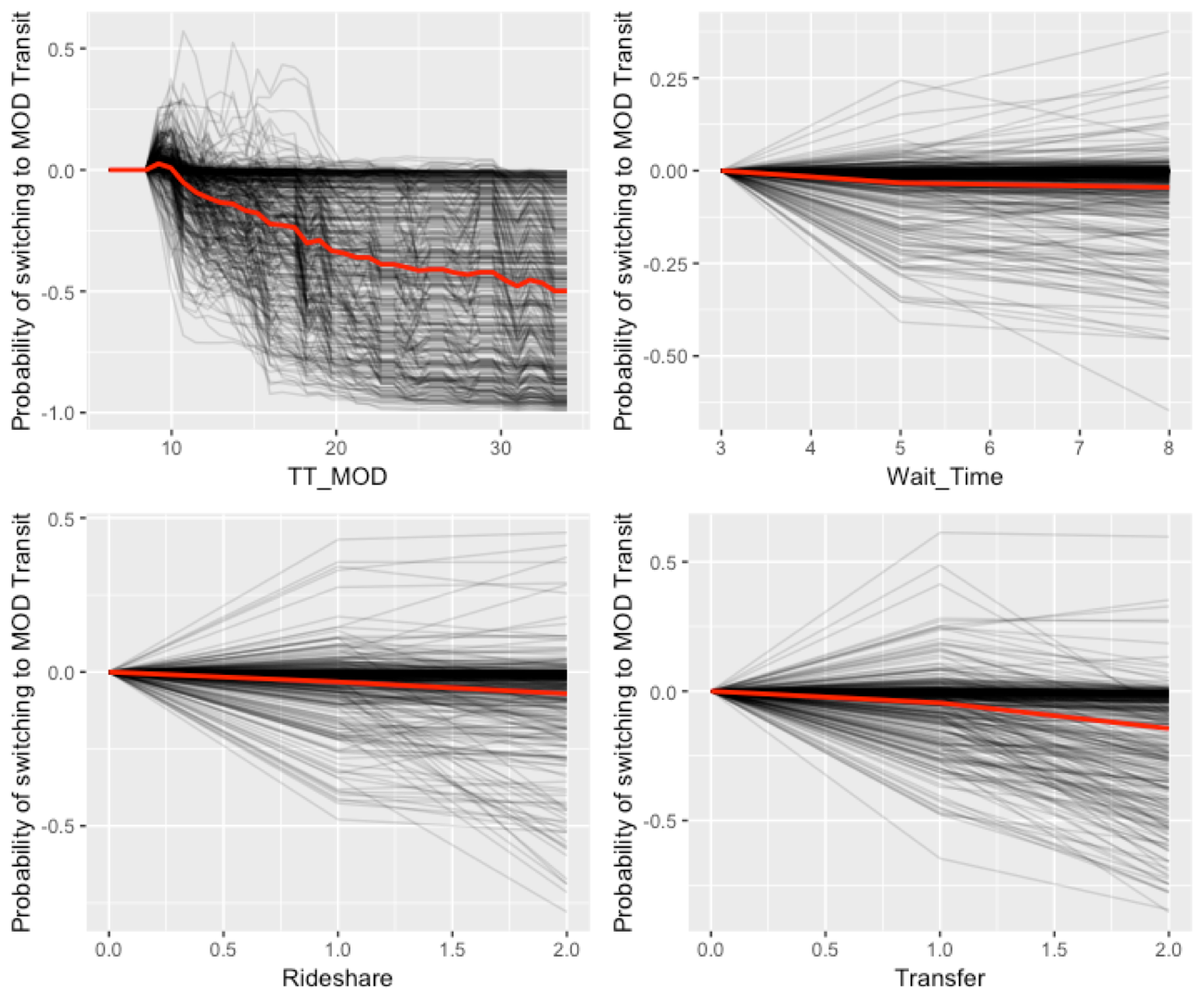
(b) C-ICE Plots

Figure 5: ICE and C-ICE Plots of Level-of-Service Variables for MOD Transit: The Red Lines Represent the Corresponding PDP.

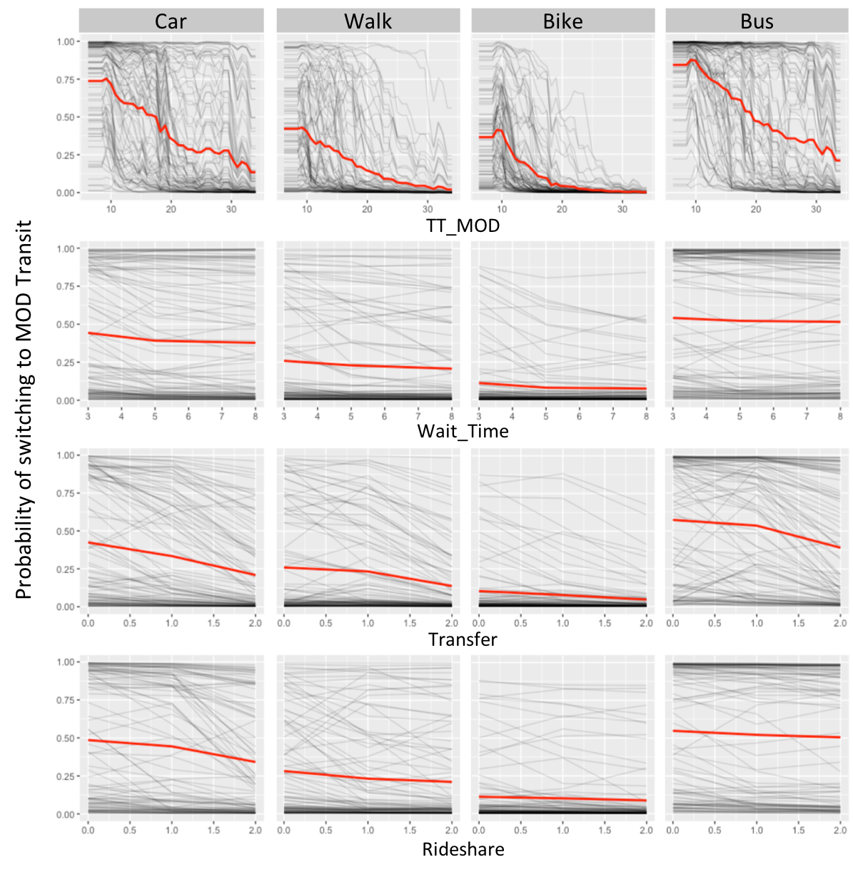
Figure 6: CIPDPs of Level-of-Service Variables for MOD Transit: The Red Lines Represent the Corresponding CPDPs.

Figure 7: Centered CIPDPs of Level-of-Service Variables for MOD Transit: The Red Lines Represent the Corresponding Centered CPDPs.

Figures 6 and 7 present the CIPDPs of different level-of-service variables for the market segments determined by the current travel mode. For TT_MOD, individuals in the Car and Bus segments exhibit more homogeneous trend of switching behavior, as all curves seem to follow the similar pattern and there are no obvious interactions. These results show that CPDPs for these two modes provide a good summary of the relationships between TT_MOD and the predicted switching probabilities well. For Walk and Bike segments, the majority of the subpopulation is following the similar trend, but there are a few individuals who behave differently from the rest of the subpopulation. For example, for Walk, the switching probabilities of several individuals do not decrease until around 30 minutes transit time.

For Wait_Time, all four market segments present response heterogeneity. Many Car users have a significant decrease in switching probability from 3 minutes to 5 minutes of waiting time, while many others do not seem to be sensitive to waiting time at all. Many walkers are similar in behavior to drivers with a few exceptions: They have a consistent decrease from 3 minutes to 8 minutes Wait_Time. For Bike users, the results are interesting: Most travelers are lumped at the bottom, showing strong intrinsic preference for not switching. On the other hand, a dozen bikers have the most decrease from 3 minutes to 5 minutes Wait_Time. Many public transit users present a steady decrease from 3 minutes to 8 minutes of waiting time, while a few of them have the most decrease from 3 minutes to 5 minutes.

For Transfer and Rideshare, significant response heterogeneity exist within and across different subpopulations. For Car users, a significant amount of individuals have a larger decrease in switching probabilities for the second Transfer/Rideshare, while some others have the most decrease for the first Transfer/Rideshare. Most walkers have a consistent decrease as Transfer changes from 0 to 2 and have the most signifcant decrease for the first Rideshare. Most bikers present no interest of switching to MOD Transit, with some of them showing a consistent decrease for Transfer and Rideshare. Lastly, most Bus users show larger decreases in switching probability on the second Transfer, while a few of them have larger decreases for the first Transfer. In terms of Rideshare, many display a consistent decrease, while some of them have the most decrease for the first additional pickup.

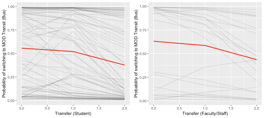
Figure 8: CIPDPs of Level-of-Service Variables for MOD Transit: Conditioning on Current Mode and Faculty/Student Status.

However, some individual responses seem to be unrealistic: Taking Transfer as an example, some individuals in Walk and Bus segments exhibit increases in switching probabilities as Transfer changes from 0 to 1, and the switching probabilities decrease significantly as Transfer changes from 1 to 2. Figure 8 applies a two-dimensional segmentation to understand this anomaly. It shows that many more anomalies for students than faculty, indicating that some students may have misreported some of their preferences. This also illustrates the benefits of CPDPs and CIPDPs in zooming on the results to build a better understanding.

With high predictive accuracy among all the market segments (over 86%) and reasonable taste heterogeneity patterns revealed above, it may be argued that the BOOST model segments the entire population and capture heterogeneity automatically; that is to say, the BOOST model accounts for individual heterogeneity by itself without explicit model-specification efforts from the modeler. This claim is consistent with the findings in Lhéritier et al. [19], which has shown that the RF model captures segments in an automated way, by comparing RF with the latent class multinomial logit model. As discussed in Subsection 4.2, BOOST, BAG, and RF are all tree-based ensemble models with some differences.

5.4 Marginal Effects and Elasticities by Current Travel Mode

As discussed in Subsection 2.2, market segmentation is a widely-used approach to reduce the large number of instances being dealt with into a manageable number of mutually-exclusive groups that share well-defined characteristics [1]. After applying market segmentation to identify different groups, it becomes possible to make predictions about their responses to various conditions and generate better-targeted policies. Therefore, this subsection applies market segmentation to marginal effects and elasticities (organized by the current travel mode), to evaluate how different subpopulations react to system changes.

Table 4 presents the marginal effects and elasticities by current travel mode for the level-of-service variables of MOD Transit. As discussed in Subsection 3.2.3, tree-based models (such as the BOOST model) cannot make “out-of-bound” predictions: Hence only the marginal effects and elasticities for the instances within the data boundary are presented. For instance, when Transfer is under evaluation, only instances with no or one transfer are considered when computing the marginal effects for one unit increase, since no data is available on three transfers. By contrast, when computing the marginal effects for one unit decrease, only those instances with one or two transfer(s) are extracted for analysis. In this analysis, Transfer, Rideshare, and Wait_Time are treated as discrete features and TT_MOD is treated as a continuous feature. Marginal effects are only computed for continuous variables, since it is not meaningful to analyze 1% increase or decrease for the discrete variables. Note also that Wait_Time uses a $-2$ unit instead of $-1$ unit because it can only take three values separated by two units.

Table 4: Marginal Effects and Elasticities for Wait_Time, Transfer, Rideshare, and TT_MOD.

Variable		$\delta$	All	Car	Walk	Bike	Bus
Wait_Time	Marginal Effects	+1 unit	$-2.12$%	$-2.95$%	$-2.42$%	$-1.79$%	$-1.45$%
		$-2$ unit	0.79%	1.68%	0.65%	0.33%	0.65%
Transfer	Marginal Effects	+1 unit	$-5.32$%	$-8.71$%	$-2.36$%	$-2.72$%	$-8.18$%
		$-1$ unit	8.68%	9.57%	5.14%	2.30%	10.19%
Rideshare	Marginal Effects	+1 unit	$-4.16$%	$-8.03$%	$-4.00$%	$-1.90$%	$-2.90$%
		$-1$ unit	3.22%	7.97%	2.43%	0.96%	2.40%
TT_MOD	Marginal Effects	+1 unit	$-2.60$%	$-2.91$%	$-2.25$%	$-2.33$%	$-2.94$%
		$-1$ unit	2.49%	2.95%	2.10%	1.60%	2.94%
	Elasticities	+10%	$-1.44$	$-1.62$	$-1.93$	$-2.88$	$-1.07$
		$-10$%	1.54	1.74	1.85	2.76	1.25

As shown in Table 4, the marginal effects of TT_MOD are largely consistent across different market segments. In the literature, in-vehicle travel time was often used as a benchmark to evaluate the penalty of other level-of-service variables [18]. This paper however uses TT_MOD as the benchmark instead. The travel time of MOD Transit consists of two parts, including in-vehicle travel time and out-of-vehicle travel time, and the out-of-vehicle travel time is typically found to have more negative impacts on choosing public transit, compared to the in-vehicle travel time [41]. Therefore, when using TT_MOD to evaluate the penalty of other variables, it is expected to have smaller values compared to previous findings in the literature (which often use in-vehicle time instead). In addition, compared to the current transit users, the elasticities of TT_MOD are larger for individuals who are currently driving, walking, and biking to work, showing their relatively lower preferences for switching to MOD Transit.

The marginal effects of Wait_Time are relatively small across different travel modes, with Car users having the largest marginal effects ($-2.95$% for +1 unit and 1.68% for $-2$ unit). As discussed above, a possible explanation is that drivers are most sensitive to out-of-vehicle travel time. In addition, the results for +1 unit and $-2$ unit display noticeable differences for marginal effects of Wait_Time. A possible reason is the strong nonlinearity of Wait_Time. In general, the penalty of Wait_Time seems small in our case study, which is consistent with our previous findings (see CPDP results for Wait_Time).

For the entire market, the marginal effect results indicate that one transfer can be converted into 2.0–3.5 minutes MOD travel time (including both in-vehicle and out-of-vehicle travel times). Even though the values are relatively small, some previous studies have similar findings (see Iseki and Taylor [18]). Rideshare has relatively smaller impacts compared to Transfer, which can be converted into 1.3–1.6 min of TT_MOD. In other words, 1 Transfer is equivalent to 2 additional pickups, which is somewhat as expected since many people may prefer a longer in-vehicle travel time for Rideshare to a shorter out-of-vehicle travel time for Transfer.

On the other hand, Transfer and Rideshare present distinct impacts on different market segments. For Car and Bus users, 1 Transfer can be converted into 3.0–3.2 minutes of TT_MOD (Car) and 2.8–3.5 minutes of TT_MOD (Bus) respectively. 1 Rideshare is equivalent to 2.7–2.8 minutes TT_MOD for drivers and 0.8–1.0 minutes of TT_MOD for public transit users. The results show that existing populations who are using motorized modes to commute are most reluctant to transfers. This is consistent with our prior observations and may be explained by an increased awareness about potential delays caused by transfers in these population segments. Moreover, Rideshare has a significant negative impact on Car users indicating, once again, that Car users may value privacy the most, while people used to share rides (e.g., Bus riders) are less affected.

By contrast, one transfer is equal to 1.0–2.4 minutes of TT_MOD for walkers and 1.2–1.4 minutes of TT_MOD for bikers. One rideshare can be converted into 1.2–1.8 minutes of TT_MOD for walkers and 0.6–0.8 minutes TT_MOD for bikers. These results are relatively small, and a possible explanation is that Walk/Bike users are more likely to be active commuters, who value sustainable transport and promote an environmentally friendly lifestyle. As a result, transfers (involving out-of-vehicle walking and waiting time) and rideshares (involving carpooling) may help reduce traffic and CO₂ emission—aligning with their values and promoting a more sustainable public transit system. Therefore, walkers and bikers are not very reluctant to take transfers or rideshares.

5.5 Summary of Key Findings

The application of various model-agnostic interpretation tools to a machine-learning model with high predictive accuracy demonstrates that significant taste heterogeneity exist within and across different subpopulations, as illustrated by market segmentation using the current travel mode. Arguably, the machine-learning model can segment the entire population and accommodate individual heterogeneity in an automated way.

In terms of behavioral insights, an important finding is that the existing Car and Bus users are more sensitive to transfers than pedestrians and cyclists. Another finding is that existing drivers are more reluctant to share rides with others, perhaps due to a higher preference for privacy.

6 Conclusion

This paper studied the potential of machine-learning classifiers to predict and explain travel mode switching behavior in heterogeneous markets. It demonstrated that machine learning significantly outperforms the logit model on a case study in terms of prediction. Moreover, the paper demonstrated that it is reasonable to claim that BOOST, the most accurate model in terms of out-of-sample prediction, automatically segments the market, providing key insights on various population segments at no cost. The paper also highlighted that the BOOST results can be interpreted by existing model-agnostic tools, such as PDPs and ICE plots. Furthermore, the paper introduced two new tools, CPDPs and CIPDPs, to extend PDPs and ICE curves to various subgroups using market segmentation. Results on the case study indicated that the machine-learning classifier and the interpretation tools may help reveal individual heterogeneity in order to facilitate decision making.

We identify three potential directions for research research. The first research avenue can addresses the fact that PDPs and ICE plots assume the independence of features under evaluation from the remaining features. However, a certain level of correlation among variables exists in nearly every real-world dataset. Taking our dataset as an example, TT_MOD is somewhat correlated with other travel time variables, since the origin-destination distance is the same. To overcome this issue, a potential direction is to apply the accumulated local effects (ALE) plot [2], by only visualizing how the model predictions change in a small “window” around a particular feature value. This idea can be applied to PDPs, ICE plots, and their generalizations proposed in the paper. It should lead to new model-agnostic interpretation tools to address this independence assumption. The second direction is to use the information gained from the PDP, ICE, CPDP, and CIPDP of black-box models to design the utility functions of the logit models automatically, thus enhancing their model performance. Lastly, there was an imbalanced classification problem in our case study, and similar problems can be found in many other previous studies that focused on travel behavior modeling, such as Hagenauer and Helbich [14], Xie et al. [40], Wang and Ross [39]. Future research should study and tackle this problem in a comprehensive and systematic way.

References

- Anable (2005) Anable, J., 2005. ‘Complacent Car Addicts’ or ‘Aspiring Environmentalists’? Identifying travel behaviour segments using attitude theory. Transport Policy 12 (1), 65–78.
- Apley (2016) Apley, D. W., 2016. Visualizing the effects of predictor variables in black box supervised learning models. arXiv preprint arXiv:1612.08468.
- Athey (2017) Athey, S., 2017. Beyond prediction: Using big data for policy problems. Science 355 (6324), 483–485.
- Bhat (2000) Bhat, C. R., 2000. Incorporating observed and unobserved heterogeneity in urban work travel mode choice modeling. Transportation Science 34 (2), 228–238.
- Bhat et al. (2016) Bhat, C. R., Astroza, S., Bhat, A. C., 2016. On allowing a general form for unobserved heterogeneity in the multiple discrete–continuous probit model: Formulation and application to tourism travel. Transportation Research Part B: Methodological 86, 223–249.
- Breiman (1996) Breiman, L., 1996. Bagging predictors. Machine Learning 24 (2), 123–140.
- Breiman (2001) Breiman, L., 2001. Random forests. Machine Learning 45 (1), 5–32.
- Breiman (2017) Breiman, L., 2017. Classification and Regression Trees. Routledge.
- Cortes and Vapnik (1995) Cortes, C., Vapnik, V., 1995. Support-vector networks. Machine Learning 20 (3), 273–297.
- Doshi-Velez and Kim (2017) Doshi-Velez, F., Kim, B., 2017. Towards a rigorous science of interpretable machine learning. arXiv preprint arXiv:1702.08608.
- Du et al. (2018) Du, M., Liu, N., Hu, X., 2018. Techniques for interpretable machine learning. arXiv preprint arXiv:1808.00033.
- Friedman (2001) Friedman, J. H., 2001. Greedy function approximation: A gradient boosting machine. Annals of Statistics, 1189–1232.
- Goldstein et al. (2015) Goldstein, A., Kapelner, A., Bleich, J., Pitkin, E., 2015. Peeking inside the black box: Visualizing statistical learning with plots of individual conditional expectation. Journal of Computational and Graphical Statistics 24 (1), 44–65.
- Hagenauer and Helbich (2017) Hagenauer, J., Helbich, M., 2017. A comparative study of machine learning classifiers for modeling travel mode choice. Expert Systems with Applications 78, 273–282.
- Hastie et al. (2001) Hastie, T., Tibshirani, R., Friedman, J., 2001. The Elements of Statistical Learning. Vol. 1. Springer series in statistics New York, NY, USA:.
- Hitge and Vanderschuren (2015) Hitge, G., Vanderschuren, M., 2015. Comparison of travel time between private car and public transport in cape town. Journal of the South African Institution of Civil Engineering 57 (3), 35–43.
- Ho (1998) Ho, T. K., 1998. The random subspace method for constructing decision forests. IEEE Transactions on Pattern Analysis and Machine Intelligence 20 (8), 832–844.
- Iseki and Taylor (2009) Iseki, H., Taylor, B. D., 2009. Not all transfers are created equal: Towards a framework relating transfer connectivity to travel behaviour. Transport Reviews 29 (6), 777–800.
- Lhéritier et al. (2018) Lhéritier, A., Bocamazo, M., Delahaye, T., Acuna-Agost, R., 2018. Airline itinerary choice modeling using machine learning. Journal of Choice Modelling.
- Li et al. (2016) Li, D., Miwa, T., Morikawa, T., Liu, P., 2016. Incorporating observed and unobserved heterogeneity in route choice analysis with sampled choice sets. Transportation Research Part C: Emerging Technologies 67, 31–46.
-
Liaw and Wiener (2002)
Liaw, A., Wiener, M., 2002. Classification and regression by
randomForest. R News 2 (3), 18–22.
URL http://CRAN.R-project.org/doc/Rnews/ - Liu et al. (2011) Liu, Y., Zhang, H. H., Wu, Y., 2011. Hard or soft classification? large-margin unified machines. Journal of the American Statistical Association 106 (493), 166–177.
- Mahéo et al. (2017) Mahéo, A., Kilby, P., Van Hentenryck, P., 2017. Benders decomposition for the design of a hub and shuttle public transit system. Transportation Science.
- McCallum et al. (1998) McCallum, A., Nigam, K., et al., 1998. A comparison of event models for naive bayes text classification. In: AAAI-98 Workshop on Learning for Text Categorization. Vol. 752. Citeseer, pp. 41–48.
-
Meyer et al. (2017)
Meyer, D., Dimitriadou, E., Hornik, K., Weingessel, A., Leisch, F., 2017.
e1071: Misc Functions of the Department of Statistics, Probability Theory
Group (Formerly: E1071), TU Wien. R package version 1.6-8.
URL https://CRAN.R-project.org/package=e1071 - Molnar (2018) Molnar, C., 2018. Interpretable Machine Learning. https://christophm.github.io/interpretable-ml-book/, https://christophm.github.io/interpretable-ml-book/.
- Murdoch et al. (2019) Murdoch, W. J., Singh, C., Kumbier, K., Abbasi-Asl, R., Yu, B., 2019. Interpretable machine learning: definitions, methods, and applications. arXiv preprint arXiv:1901.04592.
- Omrani (2015) Omrani, H., 2015. Predicting travel mode of individuals by machine learning. Transportation Research Procedia 10, 840–849.
- Quinlan (2014) Quinlan, J. R., 2014. C4. 5: Programs for Machine Learning. Elsevier.
-
R Core Team (2018)
R Core Team, 2018. R: A Language and Environment for Statistical Computing. R
Foundation for Statistical Computing, Vienna, Austria.
URL https://www.R-project.org/ -
Ridgeway (2017)
Ridgeway, G., 2017. gbm: Generalized Boosted Regression Models. R
package version 2.1.3.
URL https://CRAN.R-project.org/package=gbm -
Ripley (2016)
Ripley, B., 2016. tree: Classification and Regression Trees. R package
version 1.0-37.
URL https://CRAN.R-project.org/package=tree - Srinivasan and Mahmassani (2003) Srinivasan, K. K., Mahmassani, H. S., 2003. Analyzing heterogeneity and unobserved structural effects in route-switching behavior under atis: a dynamic kernel logit formulation. Transportation Research Part B: Methodological 37 (9), 793–814.
- Tang et al. (2015) Tang, L., Xiong, C., Zhang, L., 2015. Decision tree method for modeling travel mode switching in a dynamic behavioral process. Transportation Planning and Technology 38 (8), 833–850.
-
Venables and Ripley (2002)
Venables, W. N., Ripley, B. D., 2002. Modern Applied Statistics with S, 4th
Edition. Springer, New York, iSBN 0-387-95457-0.
URL http://www.stats.ox.ac.uk/pub/MASS4 - Vij and Walker (2016) Vij, A., Walker, J. L., 2016. How, when and why integrated choice and latent variable models are latently useful. Transportation Research Part B: Methodological 90, 192–217.
-
Wager and Athey (2018)
Wager, S., Athey, S., 2018. Estimation and inference of heterogeneous treatment
effects using random forests. Journal of the American Statistical Association
113 (523), 1228–1242.
URL https://doi.org/10.1080/01621459.2017.1319839 - Wahba (2002) Wahba, G., 2002. Soft and hard classification by reproducing kernel hilbert space methods. Proceedings of the National Academy of Sciences 99 (26), 16524–16530.
- Wang and Ross (2018) Wang, F., Ross, C. L., 2018. Machine learning travel mode choices: Comparing the performance of an extreme gradient boosting model with a multinomial logit model. Transportation Research Record: Journal of the Transportation Research Board.
- Xie et al. (2003) Xie, C., Lu, J., Parkany, E., 2003. Work travel mode choice modeling with data mining: decision trees and neural networks. Transportation Research Record: Journal of the Transportation Research Board (1854), 50–61.
-
Yan et al. (2018)
Yan, X., Levine, J., Zhao, X., 2018. Integrating ridesourcing services with
public transit: An evaluation of traveler responses combining revealed and
stated preference data. Transportation Research Part C: Emerging
Technologies.
URL http://www.sciencedirect.com/science/article/pii/S0968090X18310398 - Zhao and Hastie (2017) Zhao, Q., Hastie, T., 2017. Causal interpretations of black-box models. Journal of Business & Economic Statistics, to appear.
- Zhao et al. (2018) Zhao, X., Yan, X., Yu, A., Van Hentenryck, P., 2018. Modeling stated preference for mobility-on-demand transit: A comparison of machine learning and logit models. arXiv preprint arXiv:1811.01315.