Plethora of cluster structures on $GL_{n}$

Abstract.

We continue the study of multiple cluster structures in the rings of regular functions on $GL_{n}$, $SL_{n}$ and $\operatorname{Mat}_{n}$ that are compatible with Poisson—-Lie and Poisson-homogeneous structures. According to our initial conjecture, each class in the Belavin–Drinfeld classification of Poisson–Lie structures on semisimple complex group ${\mathcal{G}}$ corresponds to a cluster structure in ${\mathcal{O}}({\mathcal{G}})$. Here we prove this conjecture for a large subset of Belavin–Drinfeld (BD) data of $A_{n}$ type, which includes all the previously known examples. Namely, we subdivide all possible $A_{n}$ type BD data into oriented and non-oriented kinds. In the oriented case, we single out BD data satisfying a certain combinatorial condition that we call aperiodicity and prove that for any BD data of this kind there exists a regular cluster structure compatible with the corresponding Poisson–Lie bracket. In fact, we extend the aperiodicity condition to pairs of oriented BD data and prove a more general result that establishes an existence of a regular cluster structure on $SL_{n}$ compatible with a Poisson bracket homogeneous with respect to the right and left action of two copies of $SL_{n}$ equipped with two different Poisson-Lie brackets. If the aperiodicity condition is not satisfied, a compatible cluster structure has to be replaced with a generalized cluster structure. We will address this situation in future publications.

1. Introduction

In this paper we continue the systematic study of multiple cluster structures in the rings of regular functions on $GL_{n}$, $SL_{n}$ and $\operatorname{Mat}_{n}$ started in [13, 14, 15]. It follows an approach developed and implemented in [10, 11, 12] for constructing cluster structures on algebraic varieties.

Recall that given a complex algebraic Poisson variety $\left({\mathcal{M}},{\{\cdot,\cdot\}}\right)$, a compatible cluster structure ${\mathcal{C}}_{\mathcal{M}}$ on ${\mathcal{M}}$ is a collection of coordinate charts (called clusters) comprised of regular functions with simple birational transition maps between charts (called cluster transformations, see [8]) such that the logarithms of any two functions in the same chart have a constant Poisson bracket. Once found, any such chart can be used as a starting point, and our construction allows us to restore the whole ${\mathcal{C}}_{\mathcal{M}}$, provided the arising birational maps preserve regularity. Algebraic structures corresponding to ${\mathcal{C}}_{\mathcal{M}}$ (the cluster algebra and the upper cluster algebra) are closely related to the ring ${\mathcal{O}}({\mathcal{M}})$ of regular functions on $\mathcal{M}$. In fact, under certain rather mild conditions, ${\mathcal{O}}({\mathcal{M}})$ can be obtained by tensoring the upper cluster algebra with ${\mathbb{C}}$, see [12].

This construction was applied in [12, Ch. 4.3] to double Bruhat cells in semisimple Lie groups equipped with (the restriction of) the standard Poisson–Lie structure. It was shown that the resulting cluster structure coincides with the one built in [2]. The standard Poisson–Lie structure is a particular case of Poisson–Lie structures corresponding to quasi-triangular Lie bialgebras. Such structures are associated with solutions to the classical Yang–Baxter equation. Their complete classification was obtained by Belavin and Drinfeld in [1]. Solutions are parametrized by the data that consists of a continuous and a discrete components. The latter, called the Belavin–Drinfeld triple, is defined in terms of the root system of the Lie algebra of the corresponding semisimple Lie group. In [13] we conjectured that any such solution gives rise to a compatible cluster structure on this Lie group. This conjecture was verified in [4] for $SL_{5}$ and proved in [5, 6] for the simplest non-trivial Belavin–Drinfeld triple in $SL_{n}$ and in [15] for the Cremmer–Gervais case.

In this paper we extend these results to a wide class of Belavin–Drinfeld triples in $SL_{n}$. We define a subclass of oriented triples, see Section 3.1, and encode the corresponding information in a combinatorial object called a Belavin–Drinfeld graph. Our main result claims that the conjecture of [13] holds true whenever the corresponding Belavin–Drinfeld graph is acyclic. In this case the structure of the Belavin–Drinfeld graph is mirrored in the explicit construction of the initial cluster. In fact, we have proved a stronger result: given two oriented Belavin–Drinfeld triples in $SL_{n}$ we define the graph of the pair, and if this graph possesses a certain acyclicity property then the Poisson bracket defined by the pair (note that it is not Poisson–Lie anymore) gives rise to a compatible cluster structure on $SL_{n}$.

If the Belavin–Drinfeld graph has cycles then the conjecture of [13] needs to be modified: one has to consider generalized cluster structures instead of the ordinary ones. We will address Belavin–Drinfeld graphs with cycles in a separate publication.

In [17], Goodearl and Yakimov developed a uniform approach for constructing cluster algebra structures in symmetric Poisson nilpotent algebras using sequences of Poisson-prime elements in chains of Poisson unique factorization domains. These results apply to a large class of Poisson varieties, e.g., Schubert cells in Kac–Moody groups viewed as Poisson subvarieties with respect to the standard Poisson-Lie bracket. It is worth pointing out, however, that the approach of [17], in its current form, does not seem to be applicable to the situation we consider here. This is evident from the fact that for cluster structures constructed in [17], the cluster algebra and the corresponding upper cluster algebra always coincide. In contrast, as we have shown in [14], the simplest non-trivial Belavin–Drinfreld data in $SL_{3}$ results in a strict inclusion of the cluster algebra into the upper cluster algebra.

The paper is organized as follows. Section 2 contains a concise description of necessary definitions and results on cluster algebras and Poisson–Lie groups. Section 3 presents main constructions and results. The Belavin–Drinfeld graph and related combinatorial data are defined in Section 3.1. The same section contains the formulations of the main Theorems 3.2 and 3.3. An explicit construction of the initial cluster is contained in Section 3.2 and summarized in Theorem 3.4. Section 4 is dedicated to the proof of this theorem. The quiver that together with the initial cluster defines the compatible cluster structure is built in Section 3.3, see Theorem 3.8 whose proof is contained in Section 5. Section 3.4 outlines the proof of the main Theorems 3.2 and 3.3. It contains, inter alia, Theorem 3.11 that enables us to implement the induction step in the proof of an isomorphism between the constructed upper cluster algebra and the ring of regular functions on $\operatorname{Mat}_{n}$. A detailed constructive proof of this isomorphism is the subject of Section 7. Section 6 is devoted to showing that cluster structures we constructed are regular and admit a global toric action.

Our research was supported in part by the NSF research grants DMS #1362801 and DMS #1702054 (M. G.), NSF research grants DMS #1362352 and DMS-1702115 (M. S.), and ISF grants #162/12 and #1144/16 (A. V.). While working on this project, we benefited from support of the following institutions and programs: Université Claude Bernard Lyon 1 (M. S., Spring 2016), University of Notre Dame (A. V., Spring 2016), Research in Pairs Program at the Mathematisches Forschungsinstitut Oberwolfach (M. G., M. S., A. V., Summer 2016), Max Planck Institute for Mathematics, Bonn (M. G. and A. V., Fall 2016), Bernoulli Brainstorm Program at EPFL, Lausanne (M. G. and A. V., Summer 2017), Research in Paris Program at the Institut Henri Poincaré (M. G., M. S., A. V., Fall 2017), Institute Des Hautes Études Scientifiques in (M. G. and A. V., Fall 2017), Mathematical Institute of the University of Heidelberg (M. G., Spring 2017 and Summer 2018), Michigan State University (A. V., Fall 2018). This paper was finished during the joint visit of the authors to the University of Notre Dame Jerusalem Global Gateway and the University of Haifa in December 2018. We are grateful to all these institutions for their hospitality and outstanding working conditions they provided. Special thanks are due to Salvatore Stella who pointed to a mistake in the original proof of Theorem 3.4 and to Gus Schrader, Alexander Shapiro and Milen Yakimov for valuable discussions.

2. Preliminaries

2.1. Cluster structures of geometric type and compatible Poisson brackets

Let ${\mathcal{F}}$ be the field of rational functions in $N+M$ independent variables with rational coefficients. There are $M$ distinguished variables; they are denoted $x_{N+1},\dots,x_{N+M}$ and called frozen, or stable. The $(N+M)$-tuple ${\bf x}=(x_{1},\dots,\allowbreak x_{N+M})$ is called a cluster, and its elements $x_{1},\dots,x_{N}$ are called cluster variables. The quiver $Q$ is a directed multigraph on the vertices $1,\dots,N+M$ corresponding to all variables; the vertices corresponding to frozen variables are called frozen. An edge going from a vertex $i$ to a vertex $j$ is denoted $i\to j$. The pair $\Sigma=({\bf x},Q)$ is called a seed.

Given a seed as above, the adjacent cluster in direction $k$, $1\leq k\leq N$, is defined by ${\bf x}^{\prime}=({\bf x}\setminus\{x_{k}\})\cup\{x^{\prime}_{k}\}$, where the new cluster variable $x^{\prime}_{k}$ is given by the exchange relation

$$x_{k}x^{\prime}_{k}=\prod_{k\to i}x_{i}+\prod_{i\to k}x_{i}.$$

The quiver mutation of $Q$ in direction $k$ is given by the following three steps: (i) for any two-edge path $i\to k\to j$ in $Q$, $e(i,j)$ edges $i\to j$ are added, where $e(i,j)$ is the number of two-edge paths $i\to k\to j$; (ii) every edge $j\to i$ (if it exists) annihilates with an edge $i\to j$; (iii) all edges $i\to k$ and all edges $k\to i$ are reversed. The resulting quiver is denoted $Q^{\prime}=\mu_{k}(Q)$. It is sometimes convenient to represent the quiver by an $N\times(N+M)$ integer matrix $B=B(Q)$ called the exchange matrix, where $b_{ij}$ is the number of arrows $i\to j$ in $Q$. Note that the principal part of $B$ is skew-symmetric (recall that the principal part of a rectangular matrix is its maximal leading square submatrix).

Given a seed $\Sigma=({\bf x},Q)$, we say that a seed $\Sigma^{\prime}=({\bf x}^{\prime},Q^{\prime})$ is adjacent to $\Sigma$ (in direction $k$) if ${\bf x}^{\prime}$ is adjacent to ${\bf x}$ in direction $k$ and $Q^{\prime}=\mu_{k}(Q)$. Two seeds are mutation equivalent if they can be connected by a sequence of pairwise adjacent seeds. The set of all seeds mutation equivalent to $\Sigma$ is called the cluster structure (of geometric type) in ${\mathcal{F}}$ associated with $\Sigma$ and denoted by ${\mathcal{C}}(\Sigma)$; in what follows, we usually write just ${\mathcal{C}}$ instead.

Let ${\mathbb{A}}$ be a ground ring satisfying the condition

$${\mathbb{Z}}[x_{N+1},\dots,x_{N+M}]\subseteq{\mathbb{A}}\subseteq{\mathbb{Z}}[x_{N+1}^{\pm 1},\dots,x_{N+M}^{\pm 1}]$$

(we write $x^{\pm 1}$ instead of $x,x^{-1}$). Following [8, 2], we associate with ${\mathcal{C}}$ two algebras of rank $N$ over ${\mathbb{A}}$: the cluster algebra ${\mathcal{A}}={\mathcal{A}}({\mathcal{C}})$, which is the ${\mathbb{A}}$-subalgebra of ${\mathcal{F}}$ generated by all cluster variables in all seeds in ${\mathcal{C}}$, and the upper cluster algebra $\overline{{\mathcal{A}}}=\overline{{\mathcal{A}}}({\mathcal{C}})$, which is the intersection of the rings of Laurent polynomials over ${\mathbb{A}}$ in cluster variables taken over all seeds in ${\mathcal{C}}$. The famous Laurent phenomenon [9] claims the inclusion ${\mathcal{A}}({\mathcal{C}})\subseteq\overline{{\mathcal{A}}}({\mathcal{C}})$. Note that originally upper cluster algebras were defined over the ring of Laurent polynomials in frozen variables. In [16] we proved that upper cluster algebras over subrings of this ring retain all properties of usual upper cluster algebras. In what follows we assume that the ground ring is the polynomial ring in frozen variables, unless explicitly stated otherwise.

Let $V$ be a quasi-affine variety over ${\mathbb{C}}$, ${\mathbb{C}}(V)$ be the field of rational functions on $V$, and ${\mathcal{O}}(V)$ be the ring of regular functions on $V$. Let ${\mathcal{C}}$ be a cluster structure in ${\mathcal{F}}$ as above. Assume that $\{f_{1},\dots,f_{N+M}\}$ is a transcendence basis of ${\mathbb{C}}(V)$. Then the map $\varphi:x_{i}\mapsto f_{i}$, $1\leq i\leq N+M]$, can be extended to a field isomorphism $\varphi:{\mathcal{F}}_{\mathbb{C}}\to{\mathbb{C}}(V)$, where ${\mathcal{F}}_{\mathbb{C}}={\mathcal{F}}\otimes{\mathbb{C}}$ is obtained from ${\mathcal{F}}$ by extension of scalars. The pair $({\mathcal{C}},\varphi)$ is called a cluster structure in ${\mathbb{C}}(V)$ (or just a cluster structure on $V$), $\{f_{1},\dots,f_{N+M}\}$ is called a cluster in $({\mathcal{C}},\varphi)$. Occasionally, we omit direct indication of $\varphi$ and say that ${\mathcal{C}}$ is a cluster structure on $V$. A cluster structure $({\mathcal{C}},\varphi)$ is called regular if $\varphi(x)$ is a regular function for any cluster variable $x$. The two algebras defined above have their counterparts in ${\mathcal{F}}_{\mathbb{C}}$ obtained by extension of scalars; they are denoted ${\mathcal{A}}_{\mathbb{C}}$ and $\overline{{\mathcal{A}}}_{\mathbb{C}}$. If, moreover, the field isomorphism $\varphi$ can be restricted to an isomorphism of ${\mathcal{A}}_{\mathbb{C}}$ (or $\overline{{\mathcal{A}}}_{\mathbb{C}}$) and ${\mathcal{O}}(V)$, we say that ${\mathcal{A}}_{\mathbb{C}}$ (or $\overline{{\mathcal{A}}}_{\mathbb{C}}$) is naturally isomorphic to ${\mathcal{O}}(V)$.

Let ${\{\cdot,\cdot\}}$ be a Poisson bracket on the ambient field ${\mathcal{F}}$, and ${\mathcal{C}}$ be a cluster structure in ${\mathcal{F}}$. We say that the bracket and the cluster structure are compatible if, for any cluster ${\bf x}=(x_{1},\dots,x_{N+M})$, one has $\{x_{i},x_{j}\}=\omega_{ij}x_{i}x_{j}$, where $\omega_{ij}\in{\mathbb{Q}}$ are constants for all $1\leq i,j\leq N+M$. The matrix $\Omega^{{\bf x}}=(\omega_{ij})$ is called the coefficient matrix of ${\{\cdot,\cdot\}}$ (in the basis ${\bf x}$); clearly, $\Omega^{{\bf x}}$ is skew-symmetric. The notion of compatibility extends to Poisson brackets on ${\mathcal{F}}_{\mathbb{C}}$ without any changes.

Fix an arbitrary cluster ${\bf x}=(x_{1},\dots,x_{N+M})$ and define a local toric action of rank $s$ at ${\bf x}$ as a map

(2.1) $${\bf x}\mapsto\left(x_{i}\prod_{\alpha=1}^{s}q_{\alpha}^{w_{i\alpha}}\right)_{i=1}^{N+M},\qquad{\bf q}=(q_{1},\dots,q_{s})\in({\mathbb{C}}^{*})^{s},$$

where $W=(w_{i\alpha})$ is an integer $(N+M)\times s$ weight matrix of full rank. Let ${\bf x}^{\prime}$ be another cluster in ${\mathcal{C}}$, then the corresponding local toric action defined by the weight matrix $W^{\prime}$ is compatible with the local toric action (2.1) if it commutes with the sequence of cluster transformations that takes ${\bf x}$ to ${\bf x}^{\prime}$. If local toric actions at all clusters are compatible, they define a global toric action on ${\mathcal{C}}$ called the ${\mathcal{C}}$-extension of the local toric action (2.1).

2.2. Poisson–Lie groups

A reductive complex Lie group ${\mathcal{G}}$ equipped with a Poisson bracket ${\{\cdot,\cdot\}}$ is called a Poisson–Lie group if the multiplication map ${\mathcal{G}}\times{\mathcal{G}}\ni(X,Y)\mapsto XY\in{\mathcal{G}}$ is Poisson. Perhaps, the most important class of Poisson–Lie groups is the one associated with quasitriangular Lie bialgebras defined in terms of classical R-matrices (see, e. g., [3, Ch. 1], [18] and [19] for a detailed exposition of these structures).

Let $\mathfrak{g}$ be the Lie algebra corresponding to ${\mathcal{G}}$ and $\langle\cdot,\cdot\rangle$ be an invariant nondegenerate form on $\mathfrak{g}$. A classical R-matrix is an element $r\in\mathfrak{g}\otimes\mathfrak{g}$ that satisfies the classical Yang–Baxter equation (CYBE). The Poisson–Lie bracket on ${\mathcal{G}}$ that corresponds to $r$ can be written as

(2.2) $$\{f^{1},f^{2}\}_{r} =\langle R_{+}(\nabla^{L}f^{1}),\nabla^{L}f^{2}\rangle-\langle R_{+}(\nabla^{R}f^{1}),\nabla^{R}f^{2}\rangle$$

$$=\langle R_{-}(\nabla^{L}f^{1}),\nabla^{L}f^{2}\rangle-\langle R_{-}(\nabla^{R}f^{1}),\nabla^{R}f^{2}\rangle,$$

where $R_{+},R_{-}\in\operatorname{End}\mathfrak{g}$ are given by $\langle R_{+}\eta,\zeta\rangle=\langle r,\eta\otimes\zeta\rangle$, $-\langle R_{-}\zeta,\eta\rangle=\langle r,\eta\otimes\zeta\rangle$ for any $\eta,\zeta\in\mathfrak{g}$ and $\nabla^{L}$, $\nabla^{R}$ are the right and the left gradients of functions on ${\mathcal{G}}$ with respect to $\langle\cdot,\cdot\rangle$ defined by

$$\left\langle\nabla^{R}f(X),\xi\right\rangle=\left.\frac{d}{dt}\right|_{t=0}f(Xe^{t\xi}),\quad\left\langle\nabla^{L}f(X),\xi\right\rangle=\left.\frac{d}{dt}\right|_{t=0}f(e^{t\xi}X)$$

for any $\xi\in\mathfrak{g}$, $X\in{\mathcal{G}}$.

Following [18], let us recall the construction of the Drinfeld double. First, note that CYBE implies that

(2.3) $$\mathfrak{g}_{+}={\operatorname{Im}}(R_{+}),\qquad\mathfrak{g}_{-}={\operatorname{Im}}(R_{-})$$

are subalgebras in $\mathfrak{g}$. The double of $\mathfrak{g}$ is $D(\mathfrak{g})=\mathfrak{g}\oplus\mathfrak{g}$ equipped with an invariant nondegenerate bilinear form

$$\langle\langle(\xi,\eta),(\xi^{\prime},\eta^{\prime})\rangle\rangle=\langle\xi,\xi^{\prime}\rangle-\langle\eta,\eta^{\prime}\rangle.$$

Define subalgebras ${\mathfrak{d}}_{\pm}$ of $D(\mathfrak{g})$ by

(2.4) $${\mathfrak{d}}_{+}=\{(\xi,\xi){:\ }\xi\in\mathfrak{g}\},\quad{\mathfrak{d}}_{-}=\{(R_{+}(\xi),R_{-}(\xi)){:\ }\xi\in\mathfrak{g}\},$$

then ${\mathfrak{d}}_{\pm}$ are isotropic subalgebras of $D(\mathfrak{g})$ and $D(\mathfrak{g})={\mathfrak{d}}_{+}\dot{+}{\mathfrak{d}}_{-}$. In other words, $(D(\mathfrak{g}),{\mathfrak{d}}_{+},{\mathfrak{d}}_{-})$ is a Manin triple. Then the operator $R_{D}=\pi_{{\mathfrak{d}}_{+}}-\pi_{{\mathfrak{d}}_{-}}$ can be used to define a Poisson–Lie structure on $D({\mathcal{G}})={\mathcal{G}}\times{\mathcal{G}}$, the double of the group ${\mathcal{G}}$, via

(2.5) $$\{f^{1},f^{2}\}^{D}_{r}=\frac{1}{2}\left(\langle\langle R_{D}({\raisebox{2.0pt}{$\bigtriangledown$}}\negthinspace^{L}f^{1}),{\raisebox{2.0pt}{$\bigtriangledown$}}\negthinspace{{}^{L}}f^{2}\rangle\rangle-\langle\langle R_{D}({\raisebox{2.0pt}{$\bigtriangledown$}}\negthinspace^{R}f^{1}),{\raisebox{2.0pt}{$\bigtriangledown$}}\negthinspace^{R}f^{2}\rangle\rangle\right),$$

where ${\raisebox{2.0pt}{$\bigtriangledown$}}\negthinspace^{R}$ and ${\raisebox{2.0pt}{$\bigtriangledown$}}\negthinspace^{L}$ are right and left gradients with respect to $\langle\langle\cdot,\cdot\rangle\rangle$. Restriction of this bracket to ${\mathcal{G}}$ identified with the diagonal subgroup of $D({\mathcal{G}})$ (whose Lie algebra is ${\mathfrak{d}}_{+}$) coincides with the Poisson–Lie bracket ${\{\cdot,\cdot\}}_{r}$ on ${\mathcal{G}}$. Let ${\mathcal{D}}_{-}$ be the subgroup of $D({\mathcal{G}})$ that corresponds to ${\mathfrak{d}}_{-}$ Double cosets of ${\mathcal{D}}_{-}$ in $D({\mathcal{G}})$ play an important role in the description of symplectic leaves in Poisson–Lie groups ${\mathcal{G}}$ and $D({\mathcal{G}})$, see [19].

The classification of classical R-matrices for simple complex Lie groups was given by Belavin and Drinfeld in [1]. Let ${\mathcal{G}}$ be a simple complex Lie group, $\Phi$ be the root system associated with its Lie algebra $\mathfrak{g}$, $\Phi^{+}$ be the set of positive roots, and $\Pi\subset\Phi^{+}$ be the set of positive simple roots. A Belavin–Drinfeld triple $\mathbf{\Gamma}=(\Gamma_{1},\Gamma_{2},\gamma)$ (in what follows, a BD triple) consists of two subsets $\Gamma_{1},\Gamma_{2}$ of $\Pi$ and an isometry $\gamma{:\ }\Gamma_{1}\to\Gamma_{2}$ nilpotent in the following sense: for every $\alpha\in\Gamma_{1}$ there exists $m\in\mathbb{N}$ such that $\gamma^{j}(\alpha)\in\Gamma_{1}$ for $j\in[0,m-1]$, but $\gamma^{m}(\alpha)\notin\Gamma_{1}$.

The isometry $\gamma$ yields an isomorphism, also denoted by $\gamma$, between Lie subalgebras $\mathfrak{g}_{\Gamma_{1}}$ and $\mathfrak{g}_{\Gamma_{2}}$ that correspond to $\Gamma_{1}$ and $\Gamma_{2}$. It is uniquely defined by the property $\gamma e_{\alpha}=e_{\gamma(\alpha)}$ for $\alpha\in\Gamma_{1}$, where $e_{\alpha}$ is the Chevalley generator corresponding to the the root $\alpha$. The isomorphism $\gamma^{*}{:\ }\mathfrak{g}_{\Gamma_{2}}\to\mathfrak{g}_{\Gamma_{1}}$ is defined as the adjoint to $\gamma$ with respect to the form $\langle\cdot,\cdot\rangle$. It is given by $\gamma^{*}e_{\gamma(\alpha)}=e_{\alpha}$ for $\gamma(\alpha)\in\Gamma_{2}$. Both $\gamma$ and $\gamma^{*}$ can be extended to maps of $\mathfrak{g}$ to itself by applying first the orthogonal projection on $\mathfrak{g}_{\Gamma_{1}}$ (respectively, on $\mathfrak{g}_{\Gamma_{2}}$) with respect to $\langle\cdot,\cdot\rangle$; clearly, the extended maps remain adjoint to each other. Note that the restrictions of $\gamma$ and $\gamma^{*}$ to the positive and the negative nilpotent subalgebras $\mathfrak{n}_{+}$ and $\mathfrak{n}_{-}$ of $\mathfrak{g}$ are Lie algebra homomorphisms of $\mathfrak{n}_{+}$ and $\mathfrak{n}_{-}$ to themselves, and $\gamma(e_{\pm\alpha})=0$ for all $\alpha\in\Pi\setminus\Gamma_{1}$.

By the classification theorem, each classical R-matrix is equivalent to an R-matrix from a Belavin–Drinfeld class defined by a BD triple $\mathbf{\Gamma}$. Following [7], we write down an expression for the members of this class:

(2.6) $$r=\frac{1}{2}\Omega_{\mathfrak{h}}+s+\sum_{\alpha}e_{-\alpha}\otimes e_{\alpha}+\sum_{\alpha}e_{-\alpha}\wedge\frac{\gamma}{1-\gamma}e_{\alpha};$$

here the summation is over the set of all positive roots, $\Omega_{\mathfrak{h}}\in\mathfrak{h}\otimes\mathfrak{h}$ is given by $\Omega_{\mathfrak{h}}=\sum h_{\alpha}\otimes\hat{h}_{\alpha}$ where $\{h_{\alpha}\}$ is the standard basis of the Cartan subalgebra $\mathfrak{h}$, $\{\hat{h}_{\alpha}\}$ is the dual basis with respect to the restriction of $\langle\cdot,\cdot\rangle$ to $\mathfrak{h}$, and $s\in\mathfrak{h}\wedge\mathfrak{h}$ satisfies

(2.7) $$\left((1-\gamma)\alpha\otimes\mathbf{1}\right)(2s)=\left((1+\gamma)\alpha\otimes\mathbf{1}\right)\Omega_{\mathfrak{h}}$$

for any $\alpha\in\Gamma_{1}$. Solutions to (2.7) form a linear space of dimension $\frac{k_{\mathbf{\Gamma}}(k_{\mathbf{\Gamma}}-1)}{2}$ with $k_{\mathbf{\Gamma}}=|\Pi\setminus\Gamma_{1}|$. More precisely, define

(2.8) $$\mathfrak{h}_{\mathbf{\Gamma}}=\{h\in\mathfrak{h}\ :\ \alpha(h)=\beta(h)\ \mbox{if}\ \gamma^{j}(\alpha)=\beta\quad\text{for some $j$}\},$$

then $\operatorname{dim}\mathfrak{h}_{\mathbf{\Gamma}}=k_{\mathbf{\Gamma}}$, and if $s^{\prime}$ is a fixed solution of (2.7), then every other solution has a form $s=s^{\prime}+s_{0}$, where $s_{0}$ is an arbitrary element of $\mathfrak{h}_{\mathbf{\Gamma}}\wedge\mathfrak{h}_{\mathbf{\Gamma}}$. The subalgebra $\mathfrak{h}_{\mathbf{\Gamma}}$ defines a torus $\mathcal{H}_{\mathbf{\Gamma}}=\exp\mathfrak{h}_{\mathbf{\Gamma}}$ in ${\mathcal{G}}$.

Let $\pi_{>}$, $\pi_{<}$ be projections of $\mathfrak{g}$ onto $\mathfrak{n}_{+}$ and $\mathfrak{n}_{-}$, $\pi_{\mathfrak{h}}$ be the projection onto $\mathfrak{h}$. It follows from (2.6) that $R_{+}$ in (2.2) is given by

(2.9) $$R_{+}=\frac{1}{1-\gamma}\pi_{>}-\frac{\gamma^{*}}{1-\gamma^{*}}\pi_{<}+\left(\frac{1}{2}+S\right)\pi_{\mathfrak{h}},$$

where $S\in\operatorname{End}\mathfrak{h}$ is skew-symmetric with respect to the restriction of $\langle\cdot,\cdot\rangle$ to $\mathfrak{h}$ and satisfies $\langle Sh,h^{\prime}\rangle=\langle s,h\otimes h^{\prime}\rangle$ for any $h,h^{\prime}\in\mathfrak{h}$ and conditions

(2.10) $$S(1-\gamma)h_{\alpha}=\frac{1}{2}(1+\gamma)h_{\alpha}$$

for any $\alpha\in\Gamma_{1}$, translated from (2.7).

For an R-matrix given by (2.6), subalgebras $\mathfrak{g}_{\pm}$ from (2.3) are contained in parabolic subalgebras ${\mathfrak{p}}_{\pm}$ of $\mathfrak{g}$ determined by the BD triple: ${\mathfrak{p}}_{+}$ contains $\mathfrak{b}_{+}$ and all the negative root spaces in $\mathfrak{g}_{\Gamma_{1}}$, while ${\mathfrak{p}}_{-}$ contains $\mathfrak{b}_{-}$ and all the positive root spaces in $\mathfrak{g}_{\Gamma_{2}}$. Then one has

(2.11) $${\mathfrak{p}}_{+}=\mathfrak{g}_{+}\oplus\mathfrak{h}_{+},\qquad{\mathfrak{p}}_{-}=\mathfrak{g}_{-}\oplus\mathfrak{h}_{-}$$

with $\mathfrak{h}_{\pm}\subset\mathfrak{h}$. An explicit description of subalgebras $\mathfrak{h}_{\pm}$ can be found, e.g., in [19, Sect. 3.1]. Let ${\mathfrak{l}}_{\pm}$ denote the Levi component of ${\mathfrak{p}}_{\pm}$. Then ${\mathfrak{l}}_{+}=\mathfrak{g}_{\Gamma_{1}}$, ${\mathfrak{l}}_{-}=\mathfrak{g}_{\Gamma_{2}}$, and the Lie algebra isomorphism $\gamma$ described above restricts to ${\mathfrak{l}}_{+}\cap\mathfrak{g}_{+}\to{\mathfrak{l}}_{-}\cap\mathfrak{g}_{-}$. This allows to describe the subalgebra ${\mathfrak{d}}_{-}$ as

(2.12) $${\mathfrak{d}}_{-}=\{(\xi_{+},\xi_{-})){:\ }\xi_{\pm}\in\mathfrak{g}_{\pm},\ \gamma(\pi_{{\mathfrak{l}}_{+}\cap\mathfrak{g}_{+}}\xi_{+})=\pi_{{\mathfrak{l}}_{-}\cap\mathfrak{g}_{-}}\xi_{-}\}\\ \subset\{(\xi_{+},\xi_{-})){:\ }\xi_{\pm}\in\mathfrak{g}_{\pm},\ \gamma(\pi_{{\mathfrak{l}}_{+}}\xi_{+})=\pi_{{\mathfrak{l}}_{-}}\xi_{-}\},$$

where $\pi_{\cdot}$ are the projections to the corresponding subalgebras.

In what follows we will use a Poisson bracket on ${\mathcal{G}}$ that is a generalization of the bracket (2.2). Let $r,r^{\prime}$ be two classical R-matrices, and $R_{+},R^{\prime}_{+}$ be the corresponding operators, then we write

(2.13) $$\{f^{1},f^{2}\}_{r,r^{\prime}}=\langle R_{+}(\nabla^{L}f^{1}),\nabla^{L}f^{2}\rangle-\langle R^{\prime}_{+}(\nabla^{R}f^{1}),\nabla^{R}f^{2}\rangle.$$

By [18, Proposition 12.11], the above expression defines a Poisson bracket, which is not Poisson–Lie unless $r=r^{\prime}$, in which case $\{f^{1},f^{2}\}_{r,r}$ evidently coincides with $\{f^{1},f^{2}\}_{r}$. The bracket (2.13) defines a Poisson homogeneous structure on ${\mathcal{G}}$ with respect to the left and right multiplication by Poisson–Lie groups $({\mathcal{G}},{\{\cdot,\cdot\}}_{r})$ and $({\mathcal{G}},{\{\cdot,\cdot\}}_{r^{\prime}})$, respectively. The bracket on the Drinfeld double that corresponds to $\{f^{1},f^{2}\}_{r,r^{\prime}}$ is defined similarly to (2.5) via

(2.14) $$\{f^{1},f^{2}\}^{D}_{r,r^{\prime}}=\frac{1}{2}\left(\langle\langle R_{D}({\raisebox{2.0pt}{$\bigtriangledown$}}\negthinspace^{L}f^{1}),{\raisebox{2.0pt}{$\bigtriangledown$}}\negthinspace{{}^{L}}f^{2}\rangle\rangle-\langle\langle R^{\prime}_{D}({\raisebox{2.0pt}{$\bigtriangledown$}}\negthinspace^{R}f^{1}),{\raisebox{2.0pt}{$\bigtriangledown$}}\negthinspace^{R}f^{2}\rangle\rangle\right).$$

3. Main results and the outline of the proof

3.1. Combinatorial data and main results

In this paper, we only deal with $\mathfrak{g}=\mathfrak{sl}_{n}$, and hence $\Gamma_{1}$ and $\Gamma_{2}$ can be identified with subsets of $[1,n-1]$. We assume that $\mathbf{\Gamma}$ is oriented, that is, $i,i+1\in\Gamma_{1}$ implies $\gamma(i+1)=\gamma(i)+1$.

For any $i\in[1,n]$ put

$$i_{+}=\min\{j\in[1,n]\setminus\Gamma_{1}{:\ }\ j\geq i\},\qquad i_{-}=\max\{j\in[0,n]\setminus\Gamma_{1}{:\ }\ j<i\}.$$

The interval $\Delta(i)=[i_{-}+1,i_{+}]$ is called the $X$-run of $i$. Clearly, all distinct $X$-runs form a partition of $[1,n]$. The $X$-runs are numbered consecutively from left to right. For example, let $n=7$ and $\Gamma_{1}=\{1,2,4\}$, then there are four $X$-runs: $\Delta_{1}=[1,3]$, $\Delta_{2}=[4,5]$, $\Delta_{3}=[6,6]$ and $\Delta_{4}=[7,7]$. Clearly, $\Delta(2)=\Delta_{1}$, $\Delta(4)=\Delta_{2}$, etc.

In a similar way, $\Gamma_{2}$ defines another partition of $[1,n]$ into $Y$-runs $\bar{\Delta}(i)$. For example, let in the above example $\Gamma_{2}=\{1,3,4\}$, then $\bar{\Delta}_{1}=[1,2]$, $\bar{\Delta}_{2}=[3,5]$, $\bar{\Delta}_{3}=[6,6]$ and $\bar{\Delta}_{4}=[7,7]$.

Runs of length one are called trivial. The map $\gamma$ induces a bijection on the sets of nontrivial $X$-runs and $Y$-runs: we say that $\bar{\Delta}_{i}=\gamma(\Delta_{j})$ if there exists $k\in\Delta_{j}$ such that $\bar{\Delta}(\gamma(k))=\bar{\Delta}_{i}$. The inverse of the bijection $\gamma$ is denoted $\gamma^{*}$ (the reasons for this notation will become clear later). Let in the previous example $\gamma(1)=3,\gamma(2)=4,\gamma(4)=1$, then $\bar{\Delta}_{1}=\gamma(\Delta_{2})$ and $\bar{\Delta}_{2}=\gamma(\Delta_{1})$.

The BD graph $G_{\mathbf{\Gamma}}$ is defined as follows. The vertices of $G_{\mathbf{\Gamma}}$ are two copies of the set of positive simple roots identified with $[1,n-1]$. One of the sets is called the upper part of the graph, and the other is called the lower part. A vertex $i\in\Gamma_{1}$ is connected with an inclined edge to the vertex $\gamma(i)\in\Gamma_{2}$. Finally, vertices $i$ and $n-i$ in the same part are connected with a horizontal edge. If $n=2k$ and $i=n-i=k$, the corresponding horizontal edge is a loop. The BD graph for the above example is shown in Fig. 1 on the left. In the same figure on the right one finds the BD graph for the case of $SL_{6}$ with $\Gamma_{1}=\{1,3,4\}$, $\Gamma_{2}=\{2,4,5\}$ and $\gamma{:\ }i\mapsto i+1$.

Figure 1. BD graphs for aperiodic BD triples

Clearly, there are four possible types of connected components in $G_{\mathbf{\Gamma}}$: a path, a path with a loop, a path with two loops, and a cycle. We say that a BD triple $\mathbf{\Gamma}$ is aperiodic if each component in $G_{\mathbf{\Gamma}}$ is either a path or a path with a loop, and periodic otherwise. In what follows we assume that $\mathbf{\Gamma}$ is aperiodic. The case of periodic BD triples will be addressed in a separate paper.

Remark 3.1.

Let $w_{0}$ be the longest permutation in $S_{n}$. Observe that horizontal edges in both rows of the BD graph can be seen as a depiction of the action of $\left(-w_{0}\right)$ on the set of positive simple roots of $SL_{n}$. Thus the BD graph can be used to analyze the properties of the map $w_{0}\gamma w_{0}\gamma^{-1}$. A map of this kind, with the pair $(w_{0},w_{0})$ replaced by a pair of elements of the Well group satisfying certain properties dictated by the BD triple in an arbitrary reductive Lie group, was defined in [19, Sect. 5.1.1] and utilized in the description of symplectic leaves of the corresponding Poisson–Lie structure.

The main result of this paper states that the conjecture formulated in [13] holds for oriented aperiodic BD triples in $SL_{n}$. Namely,

Theorem 3.2.

For any oriented aperiodic Belavin–Drinfeld triple $\mathbf{\Gamma}=(\Gamma_{1},\Gamma_{2},\gamma)$ there exists a cluster structure ${\mathcal{C}}_{\mathbf{\Gamma}}$ on $SL_{n}$ such that

(i) the number of frozen variables is $2k_{\mathbf{\Gamma}}$, and the corresponding exchange matrix has a full rank;

(ii) ${\mathcal{C}}_{\mathbf{\Gamma}}$ is regular, and the corresponding upper cluster algebra $\overline{{\mathcal{A}}}_{\mathbb{C}}({\mathcal{C}}_{\mathbf{\Gamma}})$ is naturally isomorphic to ${\mathcal{O}}(SL_{n})$;

(iii) the global toric action of $(\mathbb{C}^{*})^{2k_{\mathbf{\Gamma}}}$ on ${\mathcal{C}}_{\mathbf{\Gamma}}$ is generated by the action of $\mathcal{H}_{\mathbf{\Gamma}}\times\mathcal{H}_{\mathbf{\Gamma}}$ on $SL_{n}$ given by $(H_{1},H_{2})(X)=H_{1}XH_{2}$;

(iv) for any solution of CYBE that belongs to the Belavin–Drinfeld class specified by $\mathbf{\Gamma}$, the corresponding Sklyanin bracket is compatible with ${\mathcal{C}}_{\mathbf{\Gamma}}$;

(v) a Poisson–Lie bracket on $SL_{n}$ is compatible with ${\mathcal{C}}_{\mathbf{\Gamma}}$ only if it is a scalar multiple of the Sklyanin bracket associated with a solution of CYBE that belongs to the Belavin–Drinfeld class specified by $\mathbf{\Gamma}$.

This result was established previously for the Cremmer–Gervais case (given by $\gamma:i\mapsto i+1$ for $1\leq i\leq n-2$) in [15] and for all cases when $k_{\mathbf{\Gamma}}=n-2$ in [5, 6].

In fact, the construction above is a particular case of a more general construction. Let $r^{\rm r}$ and $r^{\rm c}$ be two classical R-matrices that correspond to BD triples $\mathbf{\Gamma}^{{\rm r}}=(\Gamma_{1}^{\rm r},\Gamma_{2}^{\rm r},{\gamma^{\rm r}})$ and $\mathbf{\Gamma}^{{\rm c}}=(\Gamma_{1}^{\rm c},\Gamma_{2}^{\rm c},{\gamma^{\rm c}})$, which we call the row and the column BD triples, respectively.

Assume that both $\mathbf{\Gamma}^{{\rm r}}$ and $\mathbf{\Gamma}^{{\rm c}}$ are oriented. Similarly to the BD graph $G_{\mathbf{\Gamma}}$ for $\mathbf{\Gamma}$, one can define a graph $G_{\mathbf{\Gamma}^{{\rm r}},\mathbf{\Gamma}^{{\rm c}}}$ for the pair $(\mathbf{\Gamma}^{{\rm r}},\mathbf{\Gamma}^{{\rm c}})$ as follows. Take $G_{\mathbf{\Gamma}^{{\rm r}}}$ with all inclined edges directed downwards and $G_{\mathbf{\Gamma}^{{\rm c}}}$ in which all inclined edges are directed upwards. Superimpose these graphs by identifying the corresponding vertices. In the resulting graph, for every pair of vertices $i,n-i$ in either top or bottom row there are two edges joining them. We give these edges opposite orientations. If $n$ is even, then we retain only one loop at each of the two vertices labeled $\frac{n}{2}$. The result is a directed graph $G_{\mathbf{\Gamma}^{{\rm r}},\mathbf{\Gamma}^{{\rm c}}}$ on $2(n-1)$ vertices. For example, consider the case of $GL_{5}$ with $\mathbf{\Gamma}^{{\rm r}}=\left(\{1,2\},\{2,3\},1\mapsto 2,2\mapsto 3\right)$ and $\mathbf{\Gamma}^{{\rm c}}=\left(\{1,2\},\{3,4\},1\mapsto 3,2\mapsto 4\right)$. The corresponding graph $G_{\mathbf{\Gamma}^{{\rm r}},\mathbf{\Gamma}^{{\rm c}}}$ is shown on the left in Fig. 2. For horizontal edges, no direction is indicated, which means that they can be traversed in both directions. The graph shown on in Fig. 2 on the right corresponds to the case of $GL_{8}$ with $\mathbf{\Gamma}^{{\rm r}}=\left(\{2,6\},\{3,7\},2\mapsto 3,6\mapsto 7\right)$ and $\mathbf{\Gamma}^{{\rm c}}=\left(\{2,6\},\{1,5\},6\mapsto 1,2\mapsto 5\right)$.

A directed path in $G_{\mathbf{\Gamma}^{{\rm r}},\mathbf{\Gamma}^{{\rm c}}}$ is called alternating if horizontal and inclined edges in the path alternate. In particular, an edge is a (trivial) alternating path. An alternating path with coinciding endpoints and an even number of edges is called an alternating cycle. Similarly to the decomposition of $G_{\mathbf{\Gamma}}$ into connected components, we can decompose the edge set of $G_{\mathbf{\Gamma}^{{\rm r}},\mathbf{\Gamma}^{{\rm c}}}$ into a disjoint union of maximal alternating paths and alternating cycles. If the resulting collection contains no alternating cycles, we call the pair $(\mathbf{\Gamma}^{{\rm r}},\mathbf{\Gamma}^{{\rm c}})$ aperiodic; clearly, $(\mathbf{\Gamma},\mathbf{\Gamma})$ is aperiodic if and only if $\mathbf{\Gamma}$ is aperiodic. For the graph on the left in Fig. 2, the corresponding maximal paths are $41\bar{2}\bar{3}14$, $32\bar{3}\bar{2}$, $\bar{1}\bar{4}23$, and $\bar{4}\bar{1}$ (here vertices in the lower part are marked with a dash for better visualization). None of them is an alternating cycle, so the corresponding pair is aperiodic. For the graph on the right in Fig. 2, the path $62\bar{3}\bar{5}26\bar{7}\bar{1}6$ is an alternating cycle; the edges $\bar{1}\bar{7}$ and $\bar{5}\bar{3}$ are trivial alternating paths.

Figure 2. Alternating paths and cycles in $G_{\mathbf{\Gamma}^{{\rm r}},\mathbf{\Gamma}^{{\rm c}}}$

The following result generalizes the first two claims of Theorem 3.2

Theorem 3.3.

For any aperiodic pair of oriented Belavin–Drinfeld triples $(\mathbf{\Gamma}^{{\rm r}},\mathbf{\Gamma}^{{\rm c}})$ there exists a cluster structure ${\mathcal{C}}_{\mathbf{\Gamma}^{{\rm r}},\mathbf{\Gamma}^{{\rm c}}}$ on $SL_{n}$ such that

(i) the number of frozen variables is $k_{\mathbf{\Gamma}^{{\rm r}}}+k_{\mathbf{\Gamma}^{{\rm c}}}$, and the corresponding exchange matrix has a full rank;

(ii) ${\mathcal{C}}_{\mathbf{\Gamma}^{{\rm r}},\mathbf{\Gamma}^{{\rm c}}}$ is regular, and the corresponding upper cluster algebra $\overline{{\mathcal{A}}}_{\mathbb{C}}({\mathcal{C}}_{\mathbf{\Gamma}^{{\rm r}},\mathbf{\Gamma}^{{\rm c}}})$ is naturally isomorphic to ${\mathcal{O}}(SL_{n})$.

(iii) the global toric action of $({\mathbb{C}}^{*})^{k_{\mathbf{\Gamma}}^{{\rm r}}+k_{\mathbf{\Gamma}}^{{\rm c}}}$ on ${\mathcal{C}}_{\mathbf{\Gamma}^{{\rm r}},\mathbf{\Gamma}^{{\rm c}}}$ is generated by the action of $\mathcal{H}_{\mathbf{\Gamma}^{{\rm r}}}\times\mathcal{H}_{\mathbf{\Gamma}^{{\rm c}}}$ on $SL_{n}$ given by $(H_{1},H_{2})(X)=H_{1}XH_{2}$.

(iv) for any pair of solutions of CYBE that belong to the Belavin–Drinfeld classes specified by $\mathbf{\Gamma}^{{\rm r}}$ and $\mathbf{\Gamma}^{{\rm c}}$, the corresponding bracket (2.13) is compatible with ${\mathcal{C}}_{\mathbf{\Gamma}^{{\rm r}},\mathbf{\Gamma}^{{\rm c}}}$;

(v) a Poisson bracket on $SL_{n}$ is compatible with ${\mathcal{C}}_{\mathbf{\Gamma}^{{\rm r}},\mathbf{\Gamma}^{{\rm c}}}$ only if it is a scalar multiple of the bracket (2.13) associated with a pair of solutions of CYBE that belong to the Belavin–Drinfeld classes specified by $\mathbf{\Gamma}^{{\rm r}}$ and $\mathbf{\Gamma}^{{\rm c}}$.

Following the approach suggested in [15], we will construct a cluster structure on the space $\operatorname{Mat}_{n}$ of $n\times n$ matrices and derive the required properties of ${\mathcal{C}}_{\mathbf{\Gamma}^{{\rm r}},\mathbf{\Gamma}^{{\rm c}}}$ from similar features of the latter cluster structure. Note that in the case of $GL_{n}$ we also obtain a regular cluster structure with the same properties, however, in this case the ring of regular functions on $GL_{n}$ is isomorphic to the localization of the upper cluster algebra with respect to $\det X$, which is equivalent to replacing the ground ring by the corresponding localization of the polynomial ring in frozen variables. In what follows we use the same notation ${\mathcal{C}}_{\mathbf{\Gamma}^{{\rm r}},\mathbf{\Gamma}^{{\rm c}}}$ for all three cluster structures and indicate explicitly which one is meant when needed.

3.2. The basis

Consider connected components of $G_{\mathbf{\Gamma}}$ for an aperiodic $\mathbf{\Gamma}$. The choice of the endpoint of a component induces directions of its edges: the first edge is directed from the endpoint, the second one from the head of the first one, and so on. Note that for a path with a loop, each edge except for the loop gets two opposite directions. Consequently, the choice of an endpoint of a component defines a matrix built of blocks curved out from two $n\times n$ matrices of indeterminates $X=(x_{ij})$ and $Y=(y_{ij})$. Each block is defined by a horizontal directed edge, that is, an edge whose head and tail belong to the same part of the graph. The block corresponding to a horizontal edge $i\to(n-i)$ in the upper part, called an $X$-block, is the submatrix $X_{I}^{J}$ with $I=[\alpha,n]$ and $J=[1,\beta]$, where $\alpha=(n-i+1)_{-}+1$ is the leftmost point of the $X$-run containing $n-i+1$, and $\beta=i_{+}$ is the rightmost point of the $X$-run containing $i$. The entry $(n-i+1,1)$ is called the exit point of the $X$-block. Similarly, the block corresponding to a horizontal edge $i\to(n-i)$ in the lower part, called a $Y$-block, is the submatrix $Y_{\bar{I}}^{\bar{J}}$ with $\bar{I}=[1,\bar{\alpha}]$ and $\bar{J}=[\bar{\beta},n]$, where $\bar{\alpha}=i_{+}$ is the rightmost point of the $Y$-run containing $i$ and $\bar{\beta}=(n-i+1)_{-}+1$ is the leftmost point of the $Y$-run containing $n-i+1$. The entry $(1,n-i+1)$ is called the exit point of the $Y$-block. In the example shown in Fig. 1 on the left, the edge $5\to 2$ in the upper part defines the $X$-block $X_{[1,7]}^{[1,5]}$ with the exit point $(3,1)$, the edge $4\to 3$ in the lower part defines the $Y$-block $Y_{[1,5]}^{[3,7]}$ with the exit point $(1,4)$, and the edge $1\to 6$ in the upper part defines the $X$-block $X_{[7,7]}^{[1,3]}$ with the exit point $(7,1)$, see the left part of Fig. 3 where the exit points of the blocks are circled.

Figure 3. Blocks and their gluing

The number of directed edges is odd and the blocks of different types alternate; therefore, if this number equals $4b-1$, then there are $b$ blocks of each type. If there are $4b-3$ directed edges, there are $b$ blocks of one type and $b-1$ blocks of the other type. By adding at most two dummy blocks with empty sets of rows or columns at the beginning and at the end of the sequence, we may assume that the number of blocks of each type is equal, and that the first block is of $X$-type.

The blocks are glued together with the help of inclined edges whose head and tail belong to different parts of the graph. An inclined edge $i\to j$ directed downwards stipulates placing the entry $(j,n)$ of the $Y$-block defined by $j\to(n-j)$ immediately to the left of the entry $(i,1)$ of the $X$-block defined by $(n-i)\to i$. In other words, the two blocks are glued in such a way that $\Delta(\alpha)$ and $\bar{\Delta}(\bar{\alpha})=\gamma(\Delta(\alpha))$ coincide. Similarly, an inclined edge $i\to j$ directed upwards stipulates placing the entry $(n,j)$ of the $X$-block defined by $j\to(n-j)$ immediately above the entry $(1,i)$ of the $Y$-block defined by $(n-i)\to i$. In other words, the two blocks are glued in such a way that $\bar{\Delta}(\bar{\beta})$ and $\Delta(\beta)=\gamma^{*}(\bar{\Delta}(\bar{\beta}))$ coincide. Clearly, the exit points of all blocks lie on the main diagonal of the resulting matrix. For example, the directed path $5\to 2\to 4\to 3\to 1\to 6$ in the BD graph shown in Fig. 1 on the left defines the gluing shown in Fig. 3 on the right. The runs along which the blocks are glued are shown in bold. The same path traversed in the opposite direction defines a matrix glued from the blocks $X_{[1,7]}^{[1,6]}$, $Y_{[1,5]}^{[3,7]}$ and $X_{[6,7]}^{[1,3]}$.

Given an aperiodic pair $(\mathbf{\Gamma}^{{\rm r}},\mathbf{\Gamma}^{{\rm c}})$ and the decomposition of $G_{\mathbf{\Gamma}^{{\rm r}},\mathbf{\Gamma}^{{\rm c}}}$ into maximal alternating paths, the blocks are defined in a similar way. To each edge $i\to(n-i)$ in the upper part of $G_{\mathbf{\Gamma}^{{\rm r}},\mathbf{\Gamma}^{{\rm c}}}$, assign the block $X_{I}^{J}$ with $I=[\alpha,n]$ and $J=[1,\beta]$, where $\alpha=(n-i+1)_{-}(\mathbf{\Gamma}^{{\rm r}})+1$ and $\beta=i_{+}(\mathbf{\Gamma}^{{\rm c}})$ are defined by $X$-runs exactly as before except with respect to different BD triples $\mathbf{\Gamma}^{{\rm r}}$ and $\mathbf{\Gamma}^{{\rm c}}$. Similarly, the block corresponding to a horizontal edge $i\to(n-i)$ in the lower part is the submatrix $Y_{\bar{I}}^{\bar{J}}$ with $\bar{I}=[1,\bar{\alpha}]$ and $\bar{J}=[\bar{\beta},n]$, where $\bar{\alpha}=i_{+}(\mathbf{\Gamma}^{{\rm r}})$ and $\bar{\beta}=(n-i+1)_{-}(\mathbf{\Gamma}^{{\rm c}})+1$ are defined by $Y$-runs. These blocks are glued together in the same fashion as before, except that gluing of a $Y$-block to an $X$-block on the left (respectively, at the bottom) is governed by the row triple $\mathbf{\Gamma}^{{\rm r}}$ (respectively, the column triple $\mathbf{\Gamma}^{{\rm c}}$). In what follows, we will call $X-$ and $Y-$runs corresponding to $\mathbf{\Gamma}^{{\rm r}}$ (respectively, to $\mathbf{\Gamma}^{{\rm c}}$) row (respectively, column) runs.

Let ${\mathcal{L}}={\mathcal{L}}(X,Y)$ denote the matrix glued from $X$- and $Y$-blocks as explained above. It follows immediately from the construction that if ${\mathcal{L}}$ is defined by an alternating path $i_{1}\to i_{2}\to\dots\to i_{2k}$ then it is a square $N({\mathcal{L}})\times N({\mathcal{L}})$ matrix with

$$N({\mathcal{L}})=\sum_{j=1}^{k}i_{2j-1}.$$

The matrices ${\mathcal{L}}$ defined by all maximal alternating paths in $G_{\mathbf{\Gamma}^{{\rm r}},\mathbf{\Gamma}^{{\rm c}}}$ form a collection denoted ${\mathbf{L}}={\mathbf{L}}_{\mathbf{\Gamma}^{{\rm r}},\mathbf{\Gamma}^{{\rm c}}}$ (or ${\mathbf{L}}_{\mathbf{\Gamma}}$ if $\mathbf{\Gamma}^{{\rm r}}=\mathbf{\Gamma}^{{\rm c}}=\mathbf{\Gamma}$). Thus,

(i) each ${\mathcal{L}}\in{\mathbf{L}}$ is a square $N({\mathcal{L}})\times N({\mathcal{L}})$ matrix,

(ii) for any $1\leq i<j\leq n$, there is a unique pair $({\mathcal{L}}\in{\mathbf{L}},s\in[1,N({\mathcal{L}})])$ such that ${\mathcal{L}}_{ss}=y_{ij}$, and

(iii) for any $1\leq j<i\leq n$, there exists and a unique pair $({\mathcal{L}}\in{\mathbf{L}},s\in[1,N({\mathcal{L}})])$ such that ${\mathcal{L}}_{ss}=x_{ij}$.

We thus have a bijection $\mathcal{J}=\mathcal{J}_{\mathbf{\Gamma}^{{\rm r}},\mathbf{\Gamma}^{{\rm c}}}$ between $[1,n]\times[1,n]\setminus\cup_{i=1}^{n}(i,i)$ and the set of pairs $\left\{({\mathcal{L}},s):{\mathcal{L}}\in{\mathbf{L}},s\in[1,N({\mathcal{L}})]\right\}$ that takes a pair $(i,j)$, $i\neq j$, to $({\mathcal{L}}(i,j),s(i,j))$. We then define

(3.1) $${\tt f}_{ij}(X,Y)=\det{\mathcal{L}}(i,j)_{[s(i,j),N({\mathcal{L}}(i,j))]}^{[s(i,j),N({\mathcal{L}}(i,j))]},\quad i\neq j.$$

The block of ${\mathcal{L}}(i,j)$ that contains the entry $(s(i,j),s(i,j))$ is called the leading block of ${\tt f}_{ij}$.

Additionally, we define

(3.2) $${\tt f}_{ii}^{<}(X,Y)=\det X_{[i,n]}^{[i,n]},\qquad{\tt f}_{ii}^{>}(X,Y)=\det Y_{[i,n]}^{[i,n]}.$$

The leading block of ${\tt f}_{ii}^{<}$ is $X$, and the leading block of ${\tt f}_{ij}^{>}$ is $Y$. Note that (3.2) means that $s$ is extended to the diagonal via $s(i,i)=i$, while ${\mathcal{L}}(i,i)$ is not defined uniquely: it might denote either $X$ or $Y$.

Finally, we put $f_{ij}(X)={\tt f}_{ij}(X,X)$ for $i\neq j$ and $f_{ii}(X)={\tt f}_{ii}^{<}(X,X)={\tt f}_{ii}^{>}(X,X)$, and define

$$F=F_{\mathbf{\Gamma}^{{\rm r}},\mathbf{\Gamma}^{{\rm c}}}=\{f_{ij}(X):i,j\in[1,n]\}.$$

Theorem 3.4.

Let $(\mathbf{\Gamma}^{{\rm r}},\mathbf{\Gamma}^{{\rm c}})$ be an oriented aperiodic pair of BD triples, then the family $F_{\mathbf{\Gamma}^{{\rm r}},\mathbf{\Gamma}^{{\rm c}}}$ forms a log-canonical coordinate system with respect to the Poisson bracket (2.13) on $\operatorname{Mat}_{n}$ with $r=r^{{\rm r}}$ and $r^{\prime}=r^{{\rm c}}$ given by (2.6).

Remark 3.5.

A log-canonical coordinate system on $SL_{n}$ with respect to the same bracket is formed by $F_{\mathbf{\Gamma}^{{\rm r}},\mathbf{\Gamma}^{{\rm c}}}\setminus\{\det X\}$.

Although the construction of the family of functions $F_{\mathbf{\Gamma}^{{\rm r}},\mathbf{\Gamma}^{{\rm c}}}$ is admittedly ad hoc, the intuition behind it is given by the collection ${\mathbf{L}}={\mathbf{L}}_{\mathbf{\Gamma}^{{\rm r}},\mathbf{\Gamma}^{{\rm c}}}$ that does have an intrinsic meaning. Recall the observation we previously utilized in [15]: a function serving as a frozen variable in a cluster structure on a Poisson variety has a property that it is log-canonical with every cluster variable in every cluster. The vanishing locus of such a function foliates into a union of non-generic symplectic leaves. On the other hand, in many examples of Poisson varieties supporting a cluster structure, the union of generic symplectic leaves forms an open orbit of a certain natural group action. Thus, it makes sense to select semi-invariants of this group action as frozen variables. Furthermore, a global toric action on the cluster structure arising this way can be described in two equivalent ways: it is generated by an action of a commutative subgroup of the group acting on the underlying Poisson variety or, alternatively, by Hamiltonian flows generated by the frozen variables.

In our current situation, the group action is determined by the BD data $\mathbf{\Gamma}^{{\rm r}}$, $\mathbf{\Gamma}^{{\rm c}}$. Let ${\mathfrak{d}}_{-}^{\rm r}$ and ${\mathfrak{d}}_{-}^{\rm c}$ be subalgebras defined in (2.4) that correspond to $\mathbf{\Gamma}^{{\rm r}}$ and $\mathbf{\Gamma}^{{\rm c}}$, respectively, and let ${\mathcal{D}}_{-}^{\rm r}=\exp({\mathfrak{d}}_{-}^{\rm r})$ and ${\mathcal{D}}_{-}^{\rm c}=\exp({\mathfrak{d}}_{-}^{\rm c})$ be the corresponding subgroups of the double. Consider the action of ${\mathcal{D}}_{-}^{\rm r}\times{\mathcal{D}}_{-}^{\rm c}$ on the double $D(GL_{n})$ with ${\mathcal{D}}_{-}^{\rm r}$ acting on the left and ${\mathcal{D}}_{-}^{\rm c}$ acting on the right.

Proposition 3.6.

Let ${\mathcal{L}}(X,Y)\in{\mathbf{L}}_{\mathbf{\Gamma}^{{\rm r}},\mathbf{\Gamma}^{{\rm c}}}$. Then

(i) $\det{\mathcal{L}}(X,Y)$ is a semi-invariant of the action of ${\mathcal{D}}_{-}^{\rm r}\times{\mathcal{D}}_{-}^{\rm c}$ described above;

(ii) $\det{\mathcal{L}}(X,X)$ is log-canonical with all matrix entries $x_{ij}$ with respect to the Poisson bracket (2.13).

Consequently, we select the subcollection $\{\det{\mathcal{L}}(X,X):{\mathcal{L}}\in{\mathbf{L}}_{\mathbf{\Gamma}^{{\rm r}},\mathbf{\Gamma}^{{\rm c}}}\}\cup\{\det X\}\subset F_{\mathbf{\Gamma}^{{\rm r}},\mathbf{\Gamma}^{{\rm c}}}$ as the set of frozen variables.

3.3. The quiver

Let us choose the family $F_{\mathbf{\Gamma}^{{\rm r}},\mathbf{\Gamma}^{{\rm c}}}$ as the initial cluster for our cluster structure. We now define the quiver $Q_{\mathbf{\Gamma}^{{\rm r}},\mathbf{\Gamma}^{{\rm c}}}$ that corresponds to this cluster.

The quiver has $n^{2}$ vertices labeled $(i,j)$. The function attached to a vertex $(i,j)$ is $f_{ij}$. Any vertex except for $(n,n)$ is frozen if and only if its degree is at most three. The vertex $(n,n)$ is never frozen. We will show below that frozen vertices correspond bijectively to the determinants of the matrices ${\mathcal{L}}\in{\mathbf{L}}\cup\{X\}$, as suggested by Proposition 3.6.

Figure 4. The neighborhood of a vertex $(i,j)$, $1<i,j<n$

A vertex $(i,j)$ for $1<i<n$, $1<j<n$ has degree six, and its neighborhood looks as shown in Fig. 4. Here and in what follows, mutable vertices are depicted by circles, frozen vertices by squares, and vertices of unspecified nature by ellipsa.

A vertex $(1,j)$ for $1<j<n$ can have degree two, three, five, or six. If $\mathbf{\Gamma}^{{\rm c}}$ stipulates both inclined edges $(j-1)\to(k-1)$ and $j\to k$ in the graph $G_{\mathbf{\Gamma}^{{\rm r}},\mathbf{\Gamma}^{{\rm c}}}$ for some $k$, that is, if ${\gamma^{\rm c}}(k-1)=j-1$ and ${\gamma^{\rm c}}(k)=j$, then the degree of $(1,j)$ in $Q_{\mathbf{\Gamma}^{{\rm r}},\mathbf{\Gamma}^{{\rm c}}}$ equals six, and its neighborhood looks as shown in Fig. 5(a).

If $\mathbf{\Gamma}^{{\rm c}}$ stipulates only the edge $(j-1)\to(k-1)$ as above but not the other one, that is, if ${\gamma^{\rm c}}(k-1)=j-1$ and $j\notin\Gamma_{2}^{\rm c}$, the degree of $(1,j)$ in $Q_{\mathbf{\Gamma}^{{\rm r}},\mathbf{\Gamma}^{{\rm c}}}$ equals five, and its neighborhood looks as shown in Fig. 5(b).

If $\mathbf{\Gamma}^{{\rm c}}$ stipulates only the edge $j\to k$ as above but not the other one, that is, if $j-1\notin\Gamma_{2}^{\rm c}$ and ${\gamma^{\rm c}}(k)=j$, the degree of $(1,j)$ in $Q_{\mathbf{\Gamma}^{{\rm r}},\mathbf{\Gamma}^{{\rm c}}}$ equals three, and its neighborhood looks as shown in Fig. 5(c).

Finally, if $\mathbf{\Gamma}^{{\rm c}}$ does not stipulate any one of the above two inclined edges in $G_{\mathbf{\Gamma}^{{\rm r}},\mathbf{\Gamma}^{{\rm c}}}$, that is, if $j-1,j\notin\Gamma_{2}^{\rm c}$, the degree of $(1,j)$ in $Q_{\mathbf{\Gamma}^{{\rm r}},\mathbf{\Gamma}^{{\rm c}}}$ equals two, and its neighborhood looks as shown in Fig. 5(d).

Figure 5. Possible neighborhoods of a vertex $(1,j)$, $1<j<n$

Similarly, a vertex $(i,1)$ for $1<i<n$ can have degree two, three, five, or six. If $\mathbf{\Gamma}^{{\rm r}}$ stipulates both inclined edges $(i-1)\to(k-1)$ and $i\to k$ in the graph $G_{\mathbf{\Gamma}^{{\rm r}},\mathbf{\Gamma}^{{\rm c}}}$ for some $k$, that is, if ${\gamma^{\rm r}}(i-1)=k-1$ and ${\gamma^{\rm r}}(i)=k$, then the degree of $(i,1)$ in $Q_{\mathbf{\Gamma}^{{\rm r}},\mathbf{\Gamma}^{{\rm c}}}$ equals six, and its neighborhood looks as shown in Fig. 6(a).

If $\mathbf{\Gamma}^{{\rm r}}$ stipulates only the edge $(i-1)\to(k-1)$ as above but not the other one, that is, if ${\gamma^{\rm r}}(i-1)=k-1$ and $i\notin\Gamma_{1}^{\rm r}$, the degree of $(i,1)$ in $Q_{\mathbf{\Gamma}^{{\rm r}},\mathbf{\Gamma}^{{\rm c}}}$ equals five, and its neighborhood looks as shown in Fig. 6(b).

If $\mathbf{\Gamma}^{{\rm r}}$ stipulates only the edge $i\to k$ as above but not the other one, that is, if $i-1\notin\Gamma_{1}^{\rm r}$ and ${\gamma^{\rm r}}(i)=k$, the degree of $(i,1)$ in $Q_{\mathbf{\Gamma}^{{\rm r}},\mathbf{\Gamma}^{{\rm c}}}$ equals three, and its neighborhood looks as shown in Fig. 6(c).

Finally, if $\mathbf{\Gamma}^{{\rm r}}$ does not stipulate any one of the above two inclined edges in $G_{\mathbf{\Gamma}^{{\rm r}},\mathbf{\Gamma}^{{\rm c}}}$, that is, if $i-1,i\notin\Gamma_{1}^{\rm r}$, the degree of $(i,1)$ in $Q_{\mathbf{\Gamma}^{{\rm r}},\mathbf{\Gamma}^{{\rm c}}}$ equals two, and its neighborhood looks as shown in Fig. 6(d).

Figure 6. Possible neighborhoods of a vertex $(i,1)$, $1<i<n$

A vertex $(n,j)$ for $1<j<n$ can have degree four, five, or six. If $\mathbf{\Gamma}^{{\rm c}}$ stipulates both inclined edges $(k-1)\to(j-1)$ and $k\to j$ in the graph $G_{\mathbf{\Gamma}^{{\rm r}},\mathbf{\Gamma}^{{\rm c}}}$ for some $k$, that is, if ${\gamma^{\rm c}}(j-1)=k-1$ and ${\gamma^{\rm c}}(j)=k$, then the degree of $(n,j)$ in $Q_{\mathbf{\Gamma}^{{\rm r}},\mathbf{\Gamma}^{{\rm c}}}$ equals six, and its neighborhood looks as shown in Fig. 7(a).

If $\mathbf{\Gamma}^{{\rm c}}$ stipulates only the edge $(k-1)\to(j-1)$ as above but not the other one, that is, if ${\gamma^{\rm c}}(j-1)=k-1$ and $j\notin\Gamma_{1}^{\rm c}$, the degree of $(n,j)$ in $Q_{\mathbf{\Gamma}^{{\rm r}},\mathbf{\Gamma}^{{\rm c}}}$ equals five, and its neighborhood looks as shown in Fig. 7(b).

If $\mathbf{\Gamma}^{{\rm c}}$ stipulates only the edge $k\to j$ as above but not the other one, that is, if $j-1\notin\Gamma_{1}^{\rm c}$ and ${\gamma^{\rm c}}(j)=k$, the degree of $(n,j)$ in $Q_{\mathbf{\Gamma}^{{\rm r}},\mathbf{\Gamma}^{{\rm c}}}$ equals five as well, and its neighborhood looks as shown in Fig. 7(c).

Finally, if $\mathbf{\Gamma}^{{\rm c}}$ does not stipulate any one of the above two inclined edges in $G_{\mathbf{\Gamma}^{{\rm r}},\mathbf{\Gamma}^{{\rm c}}}$, that is, if $j-1,j\notin\Gamma_{1}^{\rm c}$, the degree of $(n,j)$ in $Q_{\mathbf{\Gamma}^{{\rm r}},\mathbf{\Gamma}^{{\rm c}}}$ equals four, and its neighborhood looks as shown in Fig. 7(d).

Figure 7. Possible neighborhoods of a vertex $(n,j)$, $1<j<n$

Similarly, a vertex $(i,n)$ for $1<i<n$ can have degree four, five, or six. If $\mathbf{\Gamma}^{{\rm r}}$ stipulates both inclined edges $(k-1)\to(i-1)$ and $k\to i$ in the graph $G_{\mathbf{\Gamma}^{{\rm r}},\mathbf{\Gamma}^{{\rm c}}}$ for some $k$, that is, if ${\gamma^{\rm r}}(k-1)=i-1$ and ${\gamma^{\rm r}}(k)=i$, then the degree of $(i,n)$ in $Q_{\mathbf{\Gamma}^{{\rm r}},\mathbf{\Gamma}^{{\rm c}}}$ equals six, and its neighborhood looks as shown in Fig. 8(a).

If $\mathbf{\Gamma}^{{\rm r}}$ stipulates only the edge $(k-1)\to(i-1)$ as above but not the other one, that is, if ${\gamma^{\rm r}}(k-1)=i-1$ and $i\notin\Gamma_{2}^{\rm r}$, the degree of $(i,n)$ in $Q_{\mathbf{\Gamma}^{{\rm r}},\mathbf{\Gamma}^{{\rm c}}}$ equals five, and its neighborhood looks as shown in Fig. 8(b).

If $\mathbf{\Gamma}^{{\rm r}}$ stipulates only the edge $k\to i$ as above but not the other one, that is, if $i-1\notin\Gamma_{2}^{\rm r}$ and ${\gamma^{\rm r}}(k)=i$, the degree of $(i,n)$ in $Q_{\mathbf{\Gamma}^{{\rm r}},\mathbf{\Gamma}^{{\rm c}}}$ equals five as well, and its neighborhood looks as shown in Fig. 8(c).

Finally, if $\mathbf{\Gamma}^{{\rm r}}$ does not stipulate any one of the above two inclined edges in $G_{\mathbf{\Gamma}^{{\rm r}},\mathbf{\Gamma}^{{\rm c}}}$, that is, if $i-1,i\notin\Gamma_{2}^{\rm r}$, the degree of $(i,n)$ in $Q_{\mathbf{\Gamma}^{{\rm r}},\mathbf{\Gamma}^{{\rm c}}}$ equals four, and its neighborhood looks as shown in Fig. 8(d).

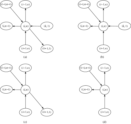
Figure 8. Possible neighborhoods of a vertex $(i,n)$, $1<i<n$

The vertex $(1,n)$ can have degree one, two, four, or five. If $\mathbf{\Gamma}^{{\rm c}}$ stipulates an inclined edge $(n-1)\to j$ for some $j$, and $\mathbf{\Gamma}^{{\rm r}}$ stipulates an inclined edge $i\to 1$ for some $i$, that is, if ${\gamma^{\rm c}}(j)=n-1$ and ${\gamma^{\rm r}}(i)=1$, then the degree of $(1,n)$ in $Q_{\mathbf{\Gamma}^{{\rm r}},\mathbf{\Gamma}^{{\rm c}}}$ equals five, and its neighborhood looks as shown in Fig. 9(a).

If only the first of the above two edges is stipulated, that is, if ${\gamma^{\rm c}}(j)=n-1$ and $1\notin\Gamma_{2}^{\rm r}$, the degree of $(1,n)$ in $Q_{\mathbf{\Gamma}^{{\rm r}},\mathbf{\Gamma}^{{\rm c}}}$ equals four, and its neighborhood looks as shown in Fig. 9(b).

If only the second of the above two edges is stipulated, that is, if ${\gamma^{\rm r}}(i)=1$ and $n-1\notin\Gamma_{2}^{\rm c}$, the degree of $(1,n)$ in $Q_{\mathbf{\Gamma}^{{\rm r}},\mathbf{\Gamma}^{{\rm c}}}$ equals two, and its neighborhood looks as shown in Fig. 9(c).

Finally, if none of the above two edges is stipulated, that is, if $1\notin\Gamma_{2}^{\rm r}$ and $n-1\notin\Gamma_{2}^{\rm c}$, the degree of $(1,n)$ in $Q_{\mathbf{\Gamma}^{{\rm r}},\mathbf{\Gamma}^{{\rm c}}}$ equals one, and its neighborhood looks as shown in Fig. 9(d).

Figure 9. Possible neighborhoods of the vertex $(1,n)$

Similarly, the vertex $(n,1)$ can have degree one, two, four, or five. If $\mathbf{\Gamma}^{{\rm r}}$ stipulates an inclined edge $(n-1)\to j$ for some $j$, and $\mathbf{\Gamma}^{{\rm c}}$ stipulates an inclined edge $i\to 1$ for some $i$, that is, if ${\gamma^{\rm r}}(n-1)=j$ and ${\gamma^{\rm c}}(1)=i$, then the degree of $(n,1)$ in $Q_{\mathbf{\Gamma}^{{\rm r}},\mathbf{\Gamma}^{{\rm c}}}$ equals five, and its neighborhood looks as shown in Fig. 10(a).

If only the first of the above two edges is stipulated, that is, if ${\gamma^{\rm r}}(n-1)=j$ and $1\notin\Gamma_{1}^{\rm c}$, the degree of $(n,1)$ in $Q_{\mathbf{\Gamma}^{{\rm r}},\mathbf{\Gamma}^{{\rm c}}}$ equals four, and its neighborhood looks as shown in Fig. 10(b).

If only the second of the above two edges is stipulated, that is, if ${\gamma^{\rm c}}(1)=i$ and $n-1\notin\Gamma_{1}^{\rm r}$, the degree of $(n,1)$ in $Q_{\mathbf{\Gamma}^{{\rm r}},\mathbf{\Gamma}^{{\rm c}}}$ equals two, and its neighborhood looks as shown in Fig. 10(c).

Finally, if none of the above two edges is stipulated, that is, if $1\notin\Gamma_{1}^{\rm c}$ and $n-1\notin\Gamma_{1}^{\rm r}$, the degree of $(n,1)$ in $Q_{\mathbf{\Gamma}^{{\rm r}},\mathbf{\Gamma}^{{\rm c}}}$ equals one, and its neighborhood looks as shown in Fig. 10(d).

Figure 10. Possible neighborhoods of the vertex $(n,1)$

The vertex $(n,n)$ can have degree three, four, or five. If $\mathbf{\Gamma}^{{\rm r}}$ stipulates an inclined edge $i\to(n-1)$ for some $i$, and $\mathbf{\Gamma}^{{\rm c}}$ stipulates an inclined edge $j\to(n-1)$ for some $j$, that is, if ${\gamma^{\rm r}}(i)=n-1$ and ${\gamma^{\rm c}}(n-1)=j$, then the degree of $(n,n)$ in $Q_{\mathbf{\Gamma}^{{\rm r}},\mathbf{\Gamma}^{{\rm c}}}$ equals five, and its neighborhood looks as shown in Fig. 11(a).

If only one of the above two edges is stipulated, that is, if either ${\gamma^{\rm r}}(i)=n-1$ and $n-1\notin\Gamma_{1}^{\rm c}$, or ${\gamma^{\rm c}}(n-1)=j$ and $n-1\notin\Gamma_{2}^{\rm r}$, the degree of $(n,n)$ in $Q_{\mathbf{\Gamma}^{{\rm r}},\mathbf{\Gamma}^{{\rm c}}}$ equals four, and its neighborhood looks as shown in Fig. 11(b,c).

Finally, if none of the above two edges is stipulated, that is, if $n-1\notin\Gamma_{1}^{\rm c}$ and $n-1\notin\Gamma_{2}^{\rm r}$, the degree of $(n,n)$ in $Q_{\mathbf{\Gamma}^{{\rm r}},\mathbf{\Gamma}^{{\rm c}}}$ equals three, and its neighborhood looks as shown in Fig. 11(d).

Figure 11. Possible neighborhoods of the vertex $(n,n)$

Finally, the vertex $(1,1)$ can have degree one, two, or three. If $\mathbf{\Gamma}^{{\rm r}}$ stipulates an inclined edge $1\to i$ for some $i$, and $\mathbf{\Gamma}^{{\rm c}}$ stipulates an inclined edge $1\to j$ for some $j$, that is, if ${\gamma^{\rm r}}(1)=i$ and ${\gamma^{\rm c}}(j)=1$, then the degree of $(1,1)$ in $Q_{\mathbf{\Gamma}^{{\rm r}},\mathbf{\Gamma}^{{\rm c}}}$ equals three, and its neighborhood looks as shown in Fig. 12(a).

If only one of the above two edges is stipulated, that is, if either ${\gamma^{\rm r}}(1)=i$ and $1\notin\Gamma_{2}^{\rm c}$, or ${\gamma^{\rm c}}(j)=1$ and $1\notin\Gamma_{1}^{\rm r}$, the degree of $(n,n)$ in $Q_{\mathbf{\Gamma}^{{\rm r}},\mathbf{\Gamma}^{{\rm c}}}$ equals two, and its neighborhood looks as shown in Fig. 12(b,c).

If none of the above two edges is stipulated, that is, if $1\notin\Gamma_{2}^{\rm c}$ and $1\notin\Gamma_{1}^{\rm r}$, the degree of $(1,1)$ in $Q_{\mathbf{\Gamma}^{{\rm r}},\mathbf{\Gamma}^{{\rm c}}}$ equals one, and its neighborhood looks as shown in Fig. 12(d).

Figure 12. Possible neighborhoods of the vertex $(1,1)$

We can now prove the characterization of frozen vertices mentioned at the beginning of the section.

Proposition 3.7.

A vertex $(i,j)$ is frozen in $Q_{\mathbf{\Gamma}^{{\rm r}},\mathbf{\Gamma}^{{\rm c}}}$ if and only if $i=j=1$ and $f_{11}=\det X$ or $f_{ij}$ is the restriction to the diagonal $X=Y$ of $\det{\mathcal{L}}$ for some ${\mathcal{L}}\in{\mathbf{L}}_{\mathbf{\Gamma}^{{\rm r}},\mathbf{\Gamma}^{{\rm c}}}$.

Proof.

It follows from the description of the quiver that there are two types of frozen vertices distinct from $(1,1)$: vertices $(1,j)$ such that $j-1\notin\Gamma^{\rm c}_{2}$, see Fig. 5(c),(d) and Fig. 9(c),(d), and vertices $(i,1)$ such that $i-1\notin\Gamma^{\rm r}_{1}$, see Fig. 6(c),(d) and Fig. 10(c),(d).

In the first case, the horizontal edge $(n-j+2)\to(j-1)$ in the lower part of $G_{\mathbf{\Gamma}^{{\rm r}},\mathbf{\Gamma}^{{\rm c}}}$ is the last edge of a maximal alternating path. Therefore, the $Y$-block defined by this edge is the uppermost block of the matrix ${\mathcal{L}}$ corresponding to this path. Consequently, $\bar{\beta}=(j-1)_{-}({\Gamma^{\rm c}})+1=j$, and hence $(1,j)$ is indeed the upper left entry of ${\mathcal{L}}$.

The second case is handled in a similar manner. ∎

The quiver $Q_{\mathbf{\Gamma}^{{\rm r}},\mathbf{\Gamma}^{{\rm c}}}$ shown in Fig. 13 corresponds to the BD data $\mathbf{\Gamma}^{{\rm r}}=\left(\{1,2\},\right.$ $\left.\{2,3\},1\mapsto 2,2\mapsto 3\right)$ and $\mathbf{\Gamma}^{{\rm c}}=\left(\{1,2\},\{3,4\},1\mapsto 3,2\mapsto 4\right)$ in $GL_{5}$. The corresponding graph $G_{\mathbf{\Gamma}^{{\rm r}},\mathbf{\Gamma}^{{\rm c}}}$ is shown on the left in Fig. 2. For example, consider the vertex $(1,4)$ and note that $G_{\mathbf{\Gamma}^{{\rm r}},\mathbf{\Gamma}^{{\rm c}}}$ contains both edges $\bar{4}\to 2$ and $\bar{3}\to 1$. Consequently, the first of the above conditions for the vertices of type $(1,j)$ holds with $k=2$, and hence $(1,4)$ has outgoing edges $(1,4)\to(5,2)$, $(1,4)\to(2,5)$, and $(1,4)\to(1,3)$, and ingoing edges $(5,1)\to(1,4)$, $(1,5)\to(1,4)$, and $(2,4)\to(1,4)$. Alternatively, consider the vertex $(4,5)$ and note that $G_{\mathbf{\Gamma}^{{\rm r}},\mathbf{\Gamma}^{{\rm c}}}$ contains the edge $2\to\bar{3}$, while $4\notin\Gamma_{2}^{\rm r}$. Consequently, the second of the above conditions for the vertices of type $(j,n)$ holds with $k=3$, and hence $(4,5)$ has outgoing edges $(4,5)\to(4,4)$ and $(4,5)\to(3,5)$ and ingoing edges $(3,4)\to(4,5)$, $(3,1)\to(4,5)$, and $(5,5)\to(4,5)$.

Figure 13. An example of the quiver $Q_{\mathbf{\Gamma}^{{\rm r}},\mathbf{\Gamma}^{{\rm c}}}$

Theorem 3.8.

Let $(\mathbf{\Gamma}^{{\rm r}},\mathbf{\Gamma}^{{\rm c}})$ be an oriented aperiodic pair of BD triples, then the quiver $Q_{\mathbf{\Gamma}^{{\rm r}},\mathbf{\Gamma}^{{\rm c}}}$ defines a cluster structure compatible with the Poisson bracket (2.13) on $\operatorname{Mat}_{n}$ with $r=r^{{\rm r}}$ and $r^{\prime}=r^{{\rm c}}$ given by (2.6).

Remark 3.9.

The quiver that defines a cluster structure compatible with the same bracket on $SL_{n}$ is obtained from $Q_{\mathbf{\Gamma}^{{\rm r}},\mathbf{\Gamma}^{{\rm c}}}$ by deleting the vertex $(1,1)$.

3.4. Outline of the proof

The proof of Theorem 3.4 is based on lengthy and rather involved calculations. Following the strategy introduced in [15], we consider the bracket (2.14) on the Drinfeld double of $SL_{n}$ and lift it to a bracket on $\operatorname{Mat}_{n}\times\operatorname{Mat}_{n}$. The family $F_{\mathbf{\Gamma}^{{\rm r}},\mathbf{\Gamma}^{{\rm c}}}$ is obtained as the restriction onto the diagonal $X=Y$ of the family ${\tt F}_{\mathbf{\Gamma}^{{\rm r}},\mathbf{\Gamma}^{{\rm c}}}$ of functions defined on $\operatorname{Mat}_{n}\times\operatorname{Mat}_{n}$ via

$${\tt F}={\tt F}_{\mathbf{\Gamma}^{{\rm r}},\mathbf{\Gamma}^{{\rm c}}}=\{{\tt f}_{ij}(X,Y):i,j\in[1,n],i\neq j\}\cup\{{\tt f}_{ii}^{<}(X,Y),{\tt f}_{ii}^{>}(X,Y):i\in[1,n]\},$$

see (3.1), (3.2). The bracket of a pair of functions $f,g\in{\tt F}_{\mathbf{\Gamma}^{{\rm r}},\mathbf{\Gamma}^{{\rm c}}}$ is decomposed into a large number of contributions that either vanish, or are proportional to the product $fg$. In the process we repeatedly use invariance properties of functions in ${\tt F}_{\mathbf{\Gamma}^{{\rm r}},\mathbf{\Gamma}^{{\rm c}}}$ with respect to the right and left action of certain subgroups of the double.

The proof of Theorem 3.8 is based on the standard characterization of Poisson structures compatible with a given cluster structure, see e.g. [12, Ch. 4]. Note that the number of frozen variables in $Q_{\mathbf{\Gamma}^{{\rm r}},\mathbf{\Gamma}^{{\rm c}}}$ equals $1+k_{\mathbf{\Gamma}^{{\rm r}}}+k_{\mathbf{\Gamma}^{{\rm c}}}$, and that $\det X$ is frozen. As an immediate consequence we get Theorem 3.3(i), which for $\mathbf{\Gamma}^{{\rm r}}=\mathbf{\Gamma}^{{\rm c}}$ turns into Theorem 3.2(i).

The proof of Theorem 3.3(iii) is based on the claim that right hand sides of all exchange relations in one cluster are semi-invariants of the left-right action of $\mathcal{H}_{\mathbf{\Gamma}^{{\rm r}}}\times\mathcal{H}_{\mathbf{\Gamma}^{{\rm c}}}$, see Lemma 6.2. It also involves the regularity check for all clusters adjacent to the initial one, see Theorem 6.1. Theorem 3.2(iii) follows when $\mathbf{\Gamma}^{{\rm r}}=\mathbf{\Gamma}^{{\rm c}}$. After this is done, Theorem 3.2(iv) and (v) follow from Theorem 3.8 via [13, Theorem 4.1]. To get Theorem 3.3(iv) and (v) we need a generalization of the latter result to the case of two different tori, which is straightforward.

The central part of the paper is the proof of Theorem 3.3(ii) (Theorem 3.2(ii) then follows in the case $\mathbf{\Gamma}^{{\rm r}}=\mathbf{\Gamma}^{{\rm c}}$). It relies on Proposition 2.1 in [15], which is reproduced below for readers’ convenience.

Proposition 3.10.

Let $V$ be a Zariski open subset in ${\mathbb{C}}^{n+m}$ and ${\mathcal{C}}$ be a cluster structure in ${\mathbb{C}}(V)$ with $n$ cluster and $m$ frozen variables such that

(i) there exists a cluster $(f_{1},\dots,f_{n+m})$ in ${\mathcal{C}}$ such that $f_{i}$ is regular on $V$ for $i\in[1,n+m]$;

(ii) any cluster variable $f_{k}^{\prime}$ adjacent to $f_{k}$, $k\in[1,n]$, is regular on $V$;

(iii) any frozen variable $f_{n+i}$, $i\in[1,m]$, vanishes at some point of $V$;

(iv) each regular function on $V$ belongs to $\overline{{\mathcal{A}}}_{\mathbb{C}}({\mathcal{C}})$.

Then ${\mathcal{C}}$ is a regular cluster structure and $\overline{{\mathcal{A}}}_{\mathbb{C}}({\mathcal{C}})$ is naturally isomorphic to ${\mathcal{O}}(V)$.

Conditions (i) and (iii) are established via direct observation, and condition (ii) was already discussed above. Therefore, the main task is to check condition (iv). Note that Theorem 3.3(i) and Theorem 3.11 in [16] imply that it is enough to check that every matrix entry can be written as a Laurent polynomial in the initial cluster and in any cluster adjacent to the initial one. In [15] this goal was achieved by constructing two distinguished sequences of mutations. Here we suggest a new approach: induction on the total size $|\Gamma^{\rm r}_{1}|+|\Gamma^{\rm c}_{1}|$. Let $\tilde{\mathbf{\Gamma}}$ be the BD triple obtained from $\mathbf{\Gamma}$ by removing a certain root $\alpha$ from $\Gamma_{1}$ and the corresponding root $\gamma(\alpha)$ from $\Gamma_{2}$. Given an aperiodic pair $(\mathbf{\Gamma}^{{\rm r}},\mathbf{\Gamma}^{{\rm c}})$ with $|\Gamma^{\rm r}_{1}|>0$, we choose $\alpha$ to be the rightmost root in an arbitrary nontrivial row $X$-run $\Delta^{\rm r}$ and define an aperiodic pair $(\tilde{\mathbf{\Gamma}}^{{\rm r}},\mathbf{\Gamma}^{{\rm c}})$. Since the total size of this pair is smaller, we assume that $\tilde{\mathcal{C}}={\mathcal{C}}_{\tilde{\mathbf{\Gamma}}^{{\rm r}},\mathbf{\Gamma}^{{\rm c}}}$ possesses the above mentioned Laurent property. Recall that both ${\mathcal{C}}$ and $\tilde{\mathcal{C}}$ are cluster structures on the space of regular functions on $\operatorname{Mat}_{n}$. To distinguish between them, the matrix entries in the latter are denoted $z_{ij}$; they form an $n\times n$ matrix $Z=(z_{ij})$.

Let $F=\{f_{ij}(X){:\ }i,j\in[1,n]\}$ and $\tilde{F}=\{\tilde{f}_{ij}(Z){:\ }i,j\in[1,n]\}$ be initial clusters for ${\mathcal{C}}$ and $\tilde{\mathcal{C}}$, respectively, and $Q$ and $\tilde{Q}$ be the corresponding quivers. It is easy to see that all maximal alternating paths in $G_{{\Gamma^{\rm r}},{\Gamma^{\rm c}}}$ are preserved in $G_{\tilde{\mathbf{\Gamma}}^{{\rm r}},\mathbf{\Gamma}^{{\rm c}}}$ except for the path that goes through the directed inclined edge $\alpha\to\gamma(\alpha)$. The latter one is split into two: the initial segment up to the vertex $\alpha$ and the closing segment starting with the vertex $\gamma(\alpha)$. Consequently, the only difference between $Q$ and $\tilde{Q}$ is that the vertex $v=(\alpha+1,1)$ that corresponds to the endpoint of the initial segment is mutable in $Q$ and frozen in $\tilde{Q}$, and that certain three edges incident to $v$ in $Q$ do not exist in $\tilde{Q}$

Let us consider four fields of rational functions in $n^{2}$ independent variables: ${\mathcal{X}}={\mathbb{C}}(x_{11},\dots,x_{nn})$, ${\mathcal{Z}}={\mathbb{C}}(z_{11},\dots,z_{nn})$, ${\mathcal{F}}={\mathbb{C}}(\varphi_{11},\dots,\varphi_{nn})$, and $\tilde{\mathcal{F}}={\mathbb{C}}(\tilde{\varphi}_{11},\dots,\allowbreak\tilde{\varphi}_{nn})$. Polynomial maps $f:{\mathcal{F}}\to{\mathcal{X}}$ and $\tilde{f}:\tilde{\mathcal{F}}\to{\mathcal{Z}}$ are given by $\varphi_{ij}\mapsto f_{ij}(X)$ and $\tilde{\varphi}_{ij}\mapsto\tilde{f}_{ij}(Z)$. By the induction hypothesis, there exists a map $\tilde{P}:{\mathcal{Z}}\to\tilde{\mathcal{F}}$ that takes $z_{ij}$ to a Laurent polynomial in variables $\tilde{\varphi}_{\alpha\beta}$ such that $\tilde{f}\circ\tilde{P}={\operatorname{Id}}$. Note that the polynomials $\tilde{f}_{ij}(Z)$ are algebraically independent, and hence $\tilde{f}$ is an isomorphism. Consequently, $\tilde{P}\circ\tilde{f}={\operatorname{Id}}$ as well. Our first goal is to build a map $P:{\mathcal{X}}\to{\mathcal{F}}$ that takes $x_{ij}$ to a Laurent polynomial in variables $\varphi_{\alpha\beta}$ and satisfies condition $f\circ P={\operatorname{Id}}$.

We start from the following result.

Theorem 3.11.

There exist a birational map $U:{\mathcal{X}}\to{\mathcal{Z}}$ and an invertible polynomial map $T:{\mathcal{F}}\to\tilde{\mathcal{F}}$ satisfying the following conditions:

a) $\tilde{f}\circ T=U\circ f$;

b) the denominator of any $U(x_{ij})$ is a power of $\tilde{f}_{v}(Z)$;

c) the inverse of $T$ is a monomial transformation.

Put $P=T^{-1}\circ\tilde{P}\circ U$; it is a map ${\mathcal{X}}\to{\mathcal{F}}$, and by a) and the induction hypothesis,

$$P\circ f=T^{-1}\circ\tilde{P}\circ U\circ f=T^{-1}\circ\tilde{P}\tilde{f}\circ T=T^{-1}\circ T={\operatorname{Id}}.$$

For the same reason as above this yields $f\circ P={\operatorname{Id}}$. Let us check that $P$ takes $x_{ij}$ to a Laurent polynomial in variables $\varphi_{\alpha\beta}$. Indeed, by b), $U$ takes $x_{ij}$ into a rational expression whose denominator is a power of $\tilde{f}_{v}(Z)$. Consequently, by the induction hypothesis, $\tilde{P}$ takes the numerator of this expression to a Laurent polynomial in $\tilde{\varphi}_{\alpha\beta}$, and the denominator to a power of $\tilde{\varphi}_{v}$. As a result, $\tilde{P}\circ U$ takes $x_{ij}$ to a Laurent polynomial in $\tilde{\varphi}_{\alpha\beta}$. Finally, by c), $T^{-1}$ takes this Laurent polynomial to a Laurent polynomial in $\varphi_{\alpha\beta}$, and hence $P$ as above satisfies the required conditions.

The next goal is to implement a similar construction at all adjacent clusters. Fix an arbitrary mutable vertex $u\neq v$ in $Q$; as it was explained above, $u$ remains mutable in $\tilde{Q}$ as well. Let $\mu_{u}(F)$ and $\mu_{u}(\tilde{F})$ be the clusters obtained from $F$ and $\tilde{F}$, respectively, via the mutation in direction $u$, and let $f^{\prime}_{u}(X)$ and $\tilde{f}^{\prime}_{u}(Z)$ be cluster variables that replace $f_{u}(X)$ and $\tilde{f}_{u}(Z)$ in $\mu_{u}(F)$ and $\mu_{u}(\tilde{F})$. Replace variables $\varphi_{u}$ and $\tilde{\varphi}_{u}$ by new variables $\varphi^{\prime}_{u}$ and $\tilde{\varphi}^{\prime}_{u}$ and define two additional fields of rational functions in $n^{2}$ variables: ${\mathcal{F}}^{\prime}={\mathbb{C}}(\varphi_{11},\dots,\varphi^{\prime}_{u},\dots,\varphi_{nn})$ and $\tilde{\mathcal{F}}^{\prime}={\mathbb{C}}(\tilde{\varphi}_{11},\dots,\tilde{\varphi}^{\prime}_{u},\dots,\tilde{\varphi}_{nn})$. Similarly to the situation discussed above, there are polynomial isomorphisms $f^{\prime}:{\mathcal{F}}^{\prime}\to{\mathcal{X}}$ and $\tilde{f}^{\prime}:\tilde{\mathcal{F}}^{\prime}\to{\mathcal{Z}}$ and a Laurent map $\tilde{P}^{\prime}:{\mathcal{Z}}\to\tilde{\mathcal{F}}^{\prime}$ such that $\tilde{f}^{\prime}\circ\tilde{P}^{\prime}={\operatorname{Id}}$ (the latter exists by the induction hypothesis).

We define a map $T^{\prime}:{\mathcal{F}}^{\prime}\to\tilde{\mathcal{F}}^{\prime}$ via $T^{\prime}(\varphi_{ij})=T(\varphi_{ij})$ for $(i,j)\neq u$ and $T^{\prime}(\varphi^{\prime}_{u})=\tilde{\varphi}^{\prime}_{u}\tilde{\varphi}_{v}^{\lambda_{u}}$ for some integer $\lambda_{u}$ and prove that maps $U$ and $T^{\prime}$ satisfy the analogs of conditions a)–c) above. Consequently, the map $P^{\prime}=(T^{\prime})^{-1}\circ\tilde{P}^{\prime}\circ U$ takes each $x_{ij}$ to a Laurent polynomial in $\varphi_{11},\dots,\varphi^{\prime}_{u},\dots,\varphi_{nn}$ and satisfies condition $P^{\prime}\circ f^{\prime}={\operatorname{Id}}$.

Thus, we proved that every matrix entry can be written as a Laurent polynomial in the initial cluster $F$ of ${\mathcal{C}}_{\mathbf{\Gamma}^{{\rm r}},\mathbf{\Gamma}^{{\rm c}}}$ and in any cluster $\mu_{u}(F)$ adjacent to it, except for the cluster $\mu_{v}(F)$. To handle this remaining cluster, we pick a different $\alpha$: the rightmost root in another nontrivial row $X$-run (if there are other nontrivial row $X$-runs), or the leftmost root of the same row $X$-run (if it differs from the rightmost root), or the rightmost root of an arbitrary nontrivial column $X$-run and an aperiodic pair $(\mathbf{\Gamma}^{{\rm r}},\tilde{\mathbf{\Gamma}}^{{\rm c}})$ (if $|\Gamma^{\rm c}_{1}|>0$), and proceed in the same way as above. Namely, we prove the existence of the analogs of the maps $U$ and $T$ satisfying conditions a)–c) above with a different distinguished vertex $v$. Consequently, $\mu_{v}(F)$ is now covered by the above reasoning about adjacent clusters.

Similarly, if the initial pair $(\mathbf{\Gamma}^{{\rm r}},\mathbf{\Gamma}^{{\rm c}})$ satisfies $|\Gamma^{\rm c}_{1}|>0$, we apply the same strategy starting with column $X$-runs. It follows from the above description that the only case that cannot be treated in this way is $|\Gamma^{\rm r}_{1}|+|\Gamma^{\rm c}_{1}|=1$. It is considered as the base of induction and treated via direct calculations

We thus obtain an analog of Theorem 3.3(ii) for the cluster structure ${\mathcal{C}}_{\mathbf{\Gamma}^{{\rm r}},\mathbf{\Gamma}^{{\rm c}}}$ on $\operatorname{Mat}_{n}$. The sought-for statement for the cluster structure on $SL_{n}$ follows from the fact that both $\overline{{\mathcal{A}}}_{\mathbb{C}}({\mathcal{C}}_{\mathbf{\Gamma}^{{\rm r}},\mathbf{\Gamma}^{{\rm c}}})$ and ${\mathcal{O}}(SL_{n})$ are obtained from their $\operatorname{Mat}_{n}$ counterparts via the restriction to $\det X=1$.

4. Initial basis

The goal of this Section is the proof of Theorem 3.4

4.1. The bracket

In this paper, we only deal with $\mathfrak{g}=\mathfrak{sl}_{n}$, and hence $\mathfrak{g}_{\Gamma_{1}}$ and $\mathfrak{g}_{\Gamma_{2}}$ are subalgebras of block-diagonal matrices with nontrivial traceless blocks determined by nontrivial runs of $\Gamma_{1}$ and $\Gamma_{2}$, respectively, and zeros everywhere else. Each diagonal component is isomorphic to $\mathfrak{sl}_{k}$, where $k$ is the size of the corresponding run. Formula (2.13), where $R_{+}=R_{+}^{\rm c}$ and $R_{+}^{\prime}=R_{+}^{\rm r}$ are given by (2.9) with $S$ skew-symmetric and subject to conditions (2.10), defines a Poisson bracket on ${\mathcal{G}}=SL_{n}$. It will be convenient to write down an extension of the bracket (2.14) to the double $D(GL_{n})$ such that its restriction to the diagonal $X=Y$ is an extension of (2.13) to $GL_{n}$ (for brevity, in what follows we write ${\{\cdot,\cdot\}}^{D}$ instead of ${\{\cdot,\cdot\}}^{D}_{r,r^{\prime}}$).

To provide an explicit expression for such an extension, we extend the maps $\gamma$ and $\gamma^{*}$ to the whole $\mathfrak{g}\mathfrak{l}_{n}$. Namely, $\gamma$ is re-defined as the projection from $\mathfrak{g}\mathfrak{l}_{n}$ onto the union of diagonal blocks specified by $\Gamma_{1}$, which are then moved by the Lie algebra isomorphism between $\mathfrak{g}_{\Gamma_{1}}$ and $\mathfrak{g}_{\Gamma_{2}}$ to corresponding diagonal blocks specified by $\Gamma_{2}$. Similarly, the adjoint map $\gamma^{*}$ acts as the projection to $\mathfrak{g}_{\Gamma_{2}}$ followed by the Lie algebra isomorphism that moves each diagonal block of $\mathfrak{g}_{\Gamma_{2}}$ back to the corresponding diagonal block of $\mathfrak{g}_{\Gamma_{1}}$. Consequently,

(4.1) $$\gamma^{*}\gamma=\Pi_{\Gamma_{1}},\qquad\gamma\gamma^{*}=\Pi_{\Gamma_{2}},$$

$$\gamma\gamma^{*}\gamma=\gamma,\qquad\gamma^{*}\gamma\gamma^{*}=\gamma^{*},$$

where $\Pi_{\Gamma_{1}}$ is the projection to $\mathfrak{g}_{\Gamma_{1}}$ and $\Pi_{\Gamma_{2}}$ is the projection to $\mathfrak{g}_{\Gamma_{2}}$. Note that the restriction of $\gamma$ to $\mathfrak{g}_{\Gamma_{1}}$ is nilpotent, and hence $1-\gamma$ is invertible on the whole $\mathfrak{g}\mathfrak{l}_{n}$.

We now view $\pi_{>}$, $\pi_{<}$ and $\pi_{0}$ as projections to the upper triangular, lower triangular and diagonal matrices, respectively. Additionally, define $\pi_{\geq}=\pi_{>}+\pi_{0}$, $\pi_{\leq}=\pi_{<}+\pi_{0}$ and for any square matrix $A$ write $A_{>}$, $A_{<}$, $A_{0}$, $A_{\geq}$, $A_{\leq}$ instead of $\pi_{>}A$, $\pi_{<}A$, $\pi_{0}A$, $\pi_{\geq}A$, $\pi_{\leq}A$, respectively. Finally, define operators $\nabla_{X}$ and $\nabla_{Y}$ via

$$\nabla_{X}f=\left(\frac{\partial f}{\partial x_{ji}}\right)_{i,j=1}^{n},\qquad\nabla_{Y}f=\left(\frac{\partial f}{\partial y_{ji}}\right)_{i,j=1}^{n},$$

and operators

$$E_{L}=\nabla_{X}X+\nabla_{Y}Y,\quad \quad E_{R}=X\nabla_{X}+Y\nabla_{Y},$$

$$\xi_{L}={\gamma^{\rm c}}(\nabla_{X}X)+\nabla_{Y}Y,\quad \quad\xi_{R}=X\nabla_{X}+{\gamma^{\rm r}}^{*}(Y\nabla_{Y}),$$

$$\eta_{L}=\nabla_{X}X+{\gamma^{\rm c}}^{*}(\nabla_{Y}Y),\quad \quad\eta_{R}={\gamma^{\rm r}}(X\nabla_{X})+Y\nabla_{Y}$$

via $E_{L}f=\nabla_{X}f\cdot X+\nabla_{Y}f\cdot Y$, $E_{R}f=X\nabla_{X}f+Y\nabla_{Y}f$, and so on. The following simple relations will be used repeatedly in what follows:

(4.2) $$\frac{1}{1-{\gamma^{\rm c}}}E_{L}=\nabla_{X}X+\frac{1}{1-{\gamma^{\rm c}}}\xi_{L}, \frac{1}{1-{\gamma^{\rm r}}}E_{R}=X\nabla_{X}+\frac{1}{1-{\gamma^{\rm r}}}\eta_{R},$$

$$\frac{1}{1-{\gamma^{\rm c}}^{*}}E_{L}=\nabla_{Y}Y+\frac{1}{1-{\gamma^{\rm c}}^{*}}\eta_{L}, \frac{1}{1-{\gamma^{\rm r}}^{*}}E_{R}=Y\nabla_{Y}+\frac{1}{1-{\gamma^{\rm r}}^{*}}\xi_{R},$$

$$\eta_{L}={\gamma^{\rm c}}^{*}(\xi_{L})+\Pi_{\hat{\Gamma}_{1}^{\rm c}}(\nabla_{X}X), \eta_{R}={\gamma^{\rm r}}(\xi_{R})+\Pi_{\hat{\Gamma}_{2}^{\rm r}}(Y\nabla_{Y}),$$

where $\Pi_{\hat{\Gamma}_{j}^{\rm l}}$ is the orthogonal projection complementary to $\Pi_{\Gamma_{j}^{\rm l}}$ for $j=1,2$, ${\rm l=r,c}$.

The statement below is a generalization of [15, Lemma 4.1].

Theorem 4.1.

The bracket (2.14) on the double $D(GL_{n})$ is given by

(4.3) $$\{f^{1},f^{2}\}^{D}(X,Y)=\left\langle R^{{\rm c}}_{+}(E_{L}f^{1}),E_{L}f^{2}\right\rangle-\left\langle R^{{\rm r}}_{+}(E_{R}f^{1}),E_{R}f^{2}\right\rangle\\ +\left\langle X\nabla_{X}f^{1},Y\nabla_{Y}f^{2}\right\rangle-\left\langle\nabla_{X}f^{1}\cdot X,\nabla_{Y}f^{2}\cdot Y\right\rangle,$$

where

(4.4) $$R^{{\rm l}}_{+}(\zeta)=\frac{1}{1-\gamma^{\rm l}}\zeta_{\geq}-\frac{{\gamma^{\rm l}}^{*}}{1-{\gamma^{\rm l}}^{*}}\zeta_{<}\\ -\frac{1}{2}\left(\frac{\gamma^{\rm l}}{1-\gamma^{\rm l}}+\frac{1}{1-{\gamma^{\rm l}}^{*}}\right)\zeta_{0}-\frac{1}{n}\left(\operatorname{Tr}(\zeta){\mathbf{S}}^{\rm l}-\operatorname{Tr}\left(\zeta{\mathbf{S}}^{\rm l}\right)\mathbf{1}\right)$$

with

$${\mathbf{S}}^{\rm l}=\frac{1}{2}\left(\frac{1}{1-\gamma^{\rm l}}-\frac{1}{1-{\gamma^{\rm l}}^{*}}\right)\mathbf{1}$$

for $\rm l=r,c$.

Proof.

We need to “tweak” $R_{+}$ to extend the bracket (2.13) to $GL_{n}$ in such a way that the function $\det$ is a Casimir function. This is guaranteed by requiring that $R_{+}$ is extended to an operator on $\mathfrak{g}\mathfrak{l}_{n}$ which coincides with the one given by (2.9) on $\mathfrak{sl}_{n}$ and for which $\mathbf{1}\in\mathfrak{g}\mathfrak{l}_{n}$ is an eigenvector. The latter goal can be achieved by replacing (2.9) with

(4.5) $$R_{+}=\frac{1}{1-\gamma}\pi_{>}-\frac{\gamma^{*}}{1-\gamma^{*}}\pi_{<}+\frac{1}{2}\pi_{0}+\pi^{*}S\pi\pi_{0},$$

where $\pi$ is the projection to the space of traceless diagonal matrices given by $\pi(\zeta)=\zeta-\frac{1}{n}\operatorname{Tr}(\zeta)\mathbf{1}$, $\pi^{*}$ is the adjoint to $\pi$ with respect to the restriction of the trace form to the space of diagonal matrices in $\mathfrak{g}\mathfrak{l}_{n}$, and $S$ is an operator on this space which is skew-symmetric with respect to the restriction of the trace form and satisfies (2.10).

The operator $S$ in (4.5) can be selected as follows.

Lemma 4.2.

The operator

(4.6) $$S=\frac{1}{2}\left(\frac{1}{1-\gamma}-\frac{1}{1-\gamma^{*}}\right)$$

with $\gamma,\gamma^{*}$ understood as acting on the space of diagonal matrices in $\mathfrak{g}\mathfrak{l}_{n}$ is skew-symmetric with respect to the restriction of the trace form to this space and satisfies (2.10).

Proof.

Rewrite (4.6) as

$$S=\frac{1}{2}\frac{1+\gamma}{1-\gamma}-\frac{1}{2}\left(\frac{\gamma}{1-\gamma}+\frac{1}{1-\gamma^{*}}\right).$$

The first term above clearly satisfies (2.10). The second term, multiplied by $(1-\gamma)$ on the right, becomes

$$-\frac{1}{2}\left(\gamma+\frac{1}{1-\gamma^{*}}(1-\gamma)\right)=-\frac{1}{2}\frac{1}{1-\gamma^{*}}\left(1-\gamma^{*}\gamma\right)$$

and vanishes on $\mathfrak{h}_{\Gamma_{1}}\subset\mathfrak{h}$ spanned by $\mathfrak{h}_{\alpha},\alpha\in\Gamma_{1}$. ∎

We can now compute

$$\pi^{*}S\pi(\zeta_{0}) =S(\zeta_{0})-\frac{1}{n}\left(\operatorname{Tr}(\zeta)S(\mathbf{1})+\operatorname{Tr}(S(\zeta_{0}))\mathbf{1}\right)$$

$$=S(\zeta_{0})-\frac{1}{n}\left(\operatorname{Tr}(\zeta)S(\mathbf{1})-\operatorname{Tr}(\zeta S(\mathbf{1}))\mathbf{1}\right)$$

and plug into (4.5) taking into account (4.6), which gives (4.4). Expression (4.3) is obtained from (2.5) in the same way as formula (4.2) in [15]. ∎

4.2. Handling functions in ${\tt F}$

It will be convenient to carry out all computations in the double with functions in ${\tt F}_{\mathbf{\Gamma}^{{\rm r}},\mathbf{\Gamma}^{{\rm c}}}$, and to retrieve the statements for $F_{\mathbf{\Gamma}^{{\rm r}},\mathbf{\Gamma}^{{\rm c}}}$ via the restriction to the diagonal.

Recall that matrices ${\mathcal{L}}$ used for the definition of the collection ${\tt F}_{\mathbf{\Gamma}^{{\rm r}},\mathbf{\Gamma}^{{\rm c}}}$ are built from $X$- and $Y$-blocks, see Section 3.2. We will frequently use the following comparison statement, which is an easy consequence of the definitions, see Fig. 14.

Proposition 4.3.

Let $X_{I}^{J}$, $X_{I^{\prime}}^{J^{\prime}}$ be two $X$-blocks and $Y_{\bar{I}}^{\bar{J}}$, $Y_{\bar{I}^{\prime}}^{\bar{J}^{\prime}}$ be two $Y$-blocks.

(i) If $\beta^{\prime}<\beta$ (respectively, $\alpha^{\prime}>\alpha$) then $X_{I^{\prime}}^{J^{\prime}}$ fits completely inside $X_{I}^{J}$; in particular, $\alpha^{\prime}\geq\alpha$ (respectively, $\beta^{\prime}\leq\beta$).

(ii) If $\bar{\beta}^{\prime}>\bar{\beta}$ (respectively, $\bar{\alpha}^{\prime}<\bar{\alpha}$) then $Y_{\bar{I}^{\prime}}^{\bar{J}^{\prime}}$ fits completely inside $Y_{\bar{I}}^{\bar{J}}$; in particular, $\bar{\alpha}^{\prime}\leq\bar{\alpha}$ (respectively, $\bar{\beta}^{\prime}\geq\bar{\beta}$).

Figure 14. Fitting of $X$- and $Y$-blocks

Consider a matrix ${\mathcal{L}}$ defined by a maximal alternating path in $G_{\mathbf{\Gamma}^{{\rm r}},\mathbf{\Gamma}^{{\rm c}}}$. Let us number the $X$-blocks along the path consecutively, so that the $t$-th $X$-block is denoted $X_{I_{t}}^{J_{t}}$. In a similar way we number the $Y$-blocks, so that the $t$-th $Y$-block is denoted $Y_{\bar{I}_{t}}^{\bar{J}_{t}}$. The glued blocks form a matrix ${\mathcal{L}}$ so that ${\mathcal{L}}_{K_{t}}^{L_{t}}=X_{I_{t}}^{J_{t}}$ and ${\mathcal{L}}_{\bar{K}_{t}}^{\bar{L}_{t}}=Y_{\bar{I}_{t}}^{\bar{J}_{t}}$, which we write as

(4.7) $${\mathcal{L}}=\sum_{t=1}^{s}X_{I_{t}\to K_{t}}^{J_{t}\to L_{t}}+\sum_{t=1}^{s}Y_{\bar{I}_{t}\to\bar{K}_{t}}^{\bar{J}_{t}\to\bar{L}_{t}}.$$

According to the agreement above, if the $t$-th $X$-block is non-dummy, then the $t$-th $Y$-block lies immediately to the left of it, and if the $t$-th $Y$-block is non-dummy, then the $(t+1)$-th $X$-block lies immediately above it. In more detail, all $K_{t}$’s are disjoint, and the same holds for all $\bar{K}_{t}$’s; moreover, $K_{t}\cap\bar{K}_{t-1}=\varnothing$. If both $t$-th blocks are not dummy, put $\Phi_{t}=K_{t}\cap\bar{K}_{t}$. Then $\Phi_{t}\neq\varnothing$ corresponds to the nontrivial row runs $\Delta(\alpha_{t})$ and $\bar{\Delta}(\bar{\alpha}_{t})=\gamma^{{\rm r}}(\Delta(\alpha_{t}))$ along which the two blocks are glued. Consequently, $\Phi_{t}$ is the uppermost segment in $K_{t}$ and the lowermost segment in $\bar{K}_{t}$. If the first block is a dummy $X$-block and $\bar{\Delta}(\bar{\alpha}_{1})$ is a nontrivial row $Y$-run, define $\Phi_{1}$ as the set of rows corresponding to $\bar{\Delta}(\bar{\alpha}_{1})$; if this $Y$-run is trivial, put $\Phi_{1}=\varnothing$. Similarly, if the last block is a dummy $Y$-block and $\Delta(\alpha_{s})$ is a nontrivial row $X$-run, define $\Phi_{s}$ as the set of rows corresponding to $\Delta(\alpha_{s})$ and put $\bar{I}_{s}={\gamma^{\rm r}}(\Delta(\alpha_{s}))$; if this $X$-run is trivial, put $\Phi_{s}=\varnothing$. We put $K_{1}=\Phi_{1}$ for a dummy first $X$-block and $\bar{K}_{s}=\Phi_{s}$ for a dummy last $Y$-block to keep relation $\Phi_{t}=K_{t}\cap\bar{K}_{t}$ valid for dummy blocks as well.

Figure 15. The structure of ${\mathcal{L}}$

Further, all $L_{t}$’s are disjoint, and the same holds for all $\bar{L}_{t}$’s; moreover, $L_{t}\cap\bar{L}_{t}=\varnothing$. For $2\leq t\leq s$, put $\Psi_{t}=L_{t}\cap\bar{L}_{t-1}$, then $\Psi_{t}\neq\varnothing$ corresponds to the nontrivial column runs $\bar{\Delta}(\bar{\beta}_{t-1})$ and $\Delta(\beta_{t})=\gamma^{{\rm c}*}(\bar{\Delta}(\bar{\beta}_{t-1}))$. Consequently, $\Psi_{t}$ is the rightmost segment in $L_{t}$ and the leftmost segment in $\bar{L}_{t-1}$. If the first block is a non-dummy $X$-block and $\Delta(\beta_{1})$ is a nontrivial column $X$-run, define $\Psi_{1}$ as the set of columns corresponding to $\Delta(\beta_{1})$; if this $X$-run is trivial, or the block is dummy, define $\Psi_{1}=\varnothing$. Similarly, if the last block is a non-dummy $Y$-block and $\bar{\Delta}(\bar{\beta}_{s})$ is a nontrivial column $Y$-run, define $\Psi_{s+1}$ as the set of columns corresponding to $\bar{\Delta}(\bar{\beta}_{s})$ and put $J_{s+1}=\gamma^{{\rm c}*}(\bar{\Delta}(\bar{\beta}_{s}))$ (note that $J_{s+1}$ does not correspond to any $X$-block of ${\mathcal{L}}$); if this $Y$-run is trivial, or the block is dummy, define $\Psi_{s+1}=\varnothing$. We put $\bar{L}_{0}=\Psi_{1}$ and $L_{s+1}=\Psi_{s+1}$ to keep relation $\Psi_{t}=L_{t}\cap\bar{L}_{t-1}$ valid for $1\leq t\leq s+1$. The structure of the obtained matrix ${\mathcal{L}}$ is shown in Fig. 15.

It follows from (4.7) that the gradients $\nabla_{X}g$ and $\nabla_{Y}g$ of a function $g=g({\mathcal{L}})$ can be written as

(4.8) $$\nabla_{X}g=\sum_{t=1}^{s}(\nabla_{{\mathcal{L}}}g)^{K_{t}\to I_{t}}_{L_{t}\to J_{t}},\qquad\nabla_{Y}g=\sum_{t=1}^{s}(\nabla_{{\mathcal{L}}}g)^{\bar{K}_{t}\to\bar{I}_{t}}_{\bar{L}_{t}\to\bar{J}_{t}}.$$

Note that unlike (4.7), the blocks in (4.8) may overlap.

Direct computation shows that for $I=[\alpha,n]$, $J=[1,\beta]$, $\bar{I}=[1,\bar{\alpha}]$, $\bar{J}=[\bar{\beta},n]$ one has

(4.9) $$X(\nabla_{{\mathcal{L}}}g)^{K\to I}_{L\to J}=\begin{bmatrix}0&\ast\\ 0&X_{I}^{J}(\nabla_{{\mathcal{L}}}g)_{L}^{K}\end{bmatrix},\qquad Y(\nabla_{{\mathcal{L}}}g)^{\bar{K}\to\bar{I}}_{\bar{L}\to\bar{J}}=\begin{bmatrix}Y_{\bar{I}}^{\bar{J}}(\nabla_{{\mathcal{L}}}g)_{\bar{L}}^{\bar{K}}&0\\ \ast&0\end{bmatrix}.$$

Here and in what follows we denote by an asterisk parts of matrices that are not relevant for further considerations. Note that the square block $X_{I}^{J}(\nabla_{{\mathcal{L}}}g)_{L}^{K}$ is the diagonal block defined by the index set $I$, whereas the square block $Y_{\bar{I}}^{\bar{J}}(\nabla_{{\mathcal{L}}}g)_{\bar{L}}^{\bar{K}}$ is the diagonal block defined by the index set $\bar{I}$.

Similarly, for $I$, $J$, $\bar{I}$, $\bar{J}$ as above,

(4.10) $$(\nabla_{{\mathcal{L}}}g)^{K\to I}_{L\to J}\cdot X=\begin{bmatrix}(\nabla_{{\mathcal{L}}}g)_{L}^{K}\cdot X_{I}^{J}&\ast\\ 0&0\end{bmatrix},\qquad(\nabla_{{\mathcal{L}}}g)^{\bar{K}\to\bar{I}}_{\bar{L}\to\bar{J}}\cdot Y=\begin{bmatrix}0&0\\ \ast&(\nabla_{{\mathcal{L}}}g)_{\bar{L}}^{\bar{K}}\cdot Y_{\bar{I}}^{\bar{J}}\end{bmatrix},$$

and the corresponding square blocks are diagonal blocks defined by the index sets $J$ and $\bar{J}$, respectively.

Let $N_{+},N_{-}\in GL_{n}$ be arbitrary unipotent upper- and lower-triangular elements and $T_{1},T_{2}\in H$ be arbitrary diagonal elements. It is easy to see that the structure of $X$- and $Y$-blocks as defined in Section 3.2 and the way they are glued together, as shown in Fig. 15, imply that for any ${\tt f}\in{{\tt F}}_{\mathbf{\Gamma}^{{\rm r}},\mathbf{\Gamma}^{{\rm c}}}$ one has

(4.11) $${\tt f}\left(N_{+}X,\exp({\gamma^{\rm r}})(N_{+})Y\right)={\tt f}\left(X\exp({\gamma^{\rm c}}^{*})(N_{-}),YN_{-}\right)={\tt f}(X,Y)$$

and

(4.12) $${\tt f}\left((T_{1}X\exp({\gamma^{\rm r}}^{*})(T_{2}),\exp({\gamma^{\rm c}})(T_{1})YT_{2}\right)=a^{\rm c}(T_{1})a^{\rm r}(T_{2}){\tt f}(X,Y),$$

where $a^{\rm c}(T_{1})$ and $a^{\rm r}(T_{2})$ are constants depending only on $T_{1}$ and $T_{2}$, respectively.

It will be more convenient to work with the logarithms of the functions ${\tt f}\in{{\tt F}}_{\mathbf{\Gamma}^{{\rm r}},\mathbf{\Gamma}^{{\rm c}}}$, instead of the functions ${\tt f}$ themselves. The corresponding infinitesimal form of the invariance properties (4.11) and (4.12) reads: for any ${\tt f}\in{{\tt F}}_{\mathbf{\Gamma}^{{\rm r}},\mathbf{\Gamma}^{{\rm c}}}$,

(4.13) $$\left\langle\xi_{R}{\tt g},n_{+}\right\rangle=\left\langle\xi_{L}{\tt g},n_{-}\right\rangle=0$$

and

(4.14) $$(\xi_{L}{\tt g})_{0}=\text{const},\quad(\xi_{R}{\tt g})_{0}=\text{const}$$

with ${\tt g}=\log{\tt f}$. Additional invariance properties of the functions in ${{\tt F}}_{\mathbf{\Gamma}^{{\rm r}},\mathbf{\Gamma}^{{\rm c}}}$ are given by the following statement.

Lemma 4.4.

For any ${\tt f}\in{{\tt F}}_{\mathbf{\Gamma}^{{\rm r}},\mathbf{\Gamma}^{{\rm c}}}$, any $X$-run $\Delta$ and any $Y$-run $\bar{\Delta}$,

$$\operatorname{Tr}(\nabla_{X}{\tt g}\cdot X)_{\Delta}^{\Delta} =\rm{const},\qquad\operatorname{Tr}(X\nabla_{X}{\tt g})_{\Delta}^{\Delta}=\rm{const},$$

$$\operatorname{Tr}(\nabla_{Y}{\tt g}\cdot Y)_{\bar{\Delta}}^{\bar{\Delta}} =\rm{const},\qquad\operatorname{Tr}(Y\nabla_{Y}{\tt g})_{\bar{\Delta}}^{\bar{\Delta}}=\rm{const}$$

with ${\tt g}=\log{\tt f}$.

Proof.

Consider for example the second equality above. Let $\mathbf{1}_{\Delta}$ denote the diagonal $n\times n$ matrix whose entry $(j,j)$ equals $1$ if $j\in\Delta$ and $0$ otherwise. Condition $\operatorname{Tr}(X\nabla_{X}{\tt g})_{\Delta}^{\Delta}=a_{\Delta}$ for an integer constant $a_{\Delta}$ is the infinitesimal version of the equality

(4.15) $${\tt f}((\mathbf{1}_{n}+(z-1)\mathbf{1}_{\Delta})X,Y)=z^{a_{\Delta}}{\tt f}(X,Y).$$

To establish the latter, recall that ${\tt f}(X,Y)$ is a principal minor of a matrix ${\mathcal{L}}\in{\mathbf{L}}$. Clearly, ${\tt f}((\mathbf{1}_{n}+(z-1)\mathbf{1}_{\Delta})X,Y)$ represents the same principal minor in the matrix ${\mathcal{L}}(z)$ obtained from ${\mathcal{L}}$ via multiplying by $z$ every submatrix ${\mathcal{L}}^{L_{t}}_{R_{t}}$ such that the row set $R_{t}$ corresponds to the $X$-run $\Delta$. There are two types of such submatrices: those for which $R_{t}$ lies strictly below $\Phi_{t}$ and those for which $R_{t}$ coincides with $\Phi_{t}$ (the latter might happen only when the run $X$ is nontrivial). To perform the above operation on each submatrix of the first type it suffices to multiply ${\mathcal{L}}$ on the left by the diagonal matrix having $z$ in all positions corresponding to $R_{t}$ and $1$ in all other positions. To handle a submatrix of the second type, we multiply by $z$ all rows of ${\mathcal{L}}$ starting from the first one and ending at the lowest row in $\bar{K}_{t}$, and divide by $z$ all columns starting from the first one and ending at the rightmost column in $\bar{L}_{t}$, see Fig. 15. Clearly, this is equivalent to the left multiplication of ${\mathcal{L}}$ by a diagonal matrix whose entries are either $z$ or $1$ and the right multiplication of ${\mathcal{L}}$ by a diagonal matrix whose entries are either $z^{-1}$ or $1$. Consequently, every principal minor of ${\mathcal{L}}(z)$ is an integer power of $z$ times the corresponding minor of ${\mathcal{L}}$, and (4.15) follows.

A similar reasoning shows that the remaining three equalities in the statement of the lemma hold as well. ∎

Furthermore, the following statement holds true.

Lemma 4.5.

For any ${\tt f}\in{{\tt F}}_{\mathbf{\Gamma}^{{\rm r}},\mathbf{\Gamma}^{{\rm c}}}$,

(4.16) $$\Pi_{\hat{\Gamma}_{1}^{\rm l}}(\nabla_{X}{\tt g}\cdot X)_{0} =\rm{const},\qquad\Pi_{\hat{\Gamma}_{1}^{\rm l}}(X\nabla_{X}{\tt g})_{0}=\rm{const},$$

$$\Pi_{\hat{\Gamma}_{2}^{\rm l}}(\nabla_{Y}{\tt g}\cdot Y)_{0} =\rm{const},\qquad\Pi_{\hat{\Gamma}_{2}^{\rm l}}(Y\nabla_{Y}{\tt g})_{0}=\rm{const}$$

with ${\tt g}=\log{\tt f}$ and ${\rm l}={\rm c},{\rm r}$.

Proof.

Same as in the proof of Lemma 4.4, we will only focus on the second equality in (4.16), since the other three can be treated in a similar way.

For any diagonal matrix $\zeta$ we have

(4.17) $$\Pi_{\hat{\Gamma}_{1}^{\rm l}}(\zeta)=\sum_{\Delta}\frac{1}{|\Delta|}\operatorname{Tr}(\zeta_{\Delta}^{\Delta})\mathbf{1}_{\Delta},$$

where the sum is taken over all $X$-runs. Let $\zeta=(X\nabla_{X}{\tt g})_{0}$, then by Lemma 4.4 all terms in the sum above are constant. ∎

Corollary 4.6.

(i) For any ${\tt f}^{i}\in{{\tt F}}_{\mathbf{\Gamma}^{{\rm r}},\mathbf{\Gamma}^{{\rm c}}}$,

(4.18) $$\operatorname{Tr}(\nabla_{X}{\tt g}\cdot X)=\rm{const},\qquad\operatorname{Tr}(X\nabla_{X}{\tt g})=\rm{const},$$

$$\operatorname{Tr}(\nabla_{Y}{\tt g}\cdot Y)=\rm{const},\qquad\operatorname{Tr}(Y\nabla_{Y}{\tt g})=\rm{const}$$

with ${\tt g}=\log{\tt f}$.

(ii) For any ${\tt f}\in{{\tt F}}_{\mathbf{\Gamma}^{{\rm r}},\mathbf{\Gamma}^{{\rm c}}}$,

(4.19) $$(\eta_{L}{\tt g})_{0}=\rm{const},\qquad(\eta_{R}{\tt g})_{0}=\rm{const}$$

with ${\tt g}=\log{\tt f}$.

Proof.

(i) Follows immediately form Lemma 4.5 and equality $\operatorname{Tr}\zeta=\operatorname{Tr}\Pi_{\hat{\Gamma}_{1}^{\rm l}}(\zeta)=\operatorname{Tr}\Pi_{\hat{\Gamma}_{2}^{\rm l}}(\zeta)$ for any $\zeta$ and ${\rm l}={\rm c},{\rm r}$.

(ii) Follows immediately form Lemma 4.5 and (4.14) via the last two relations in (4.2). ∎

4.3. Proof of Theorem 3.4: first steps

Theorem 3.4 is an immediate corollary of the following result.

Theorem 4.7.

For any ${\tt f}^{1},{\tt f}^{2}\in{{\tt F}}_{\mathbf{\Gamma}^{{\rm r}},\mathbf{\Gamma}^{{\rm c}}}$, the bracket $\{\log{\tt f}^{1},\log{\tt f}^{2}\}^{D}$ is constant.

The proof of the theorem is given in this and the following sections. It comprises a number of explicit formulas for the objects involved.

4.3.1. Explicit expression for the bracket

Let us derive an explicit expression for $\{\log{\tt f}^{1},\log{\tt f}^{2}\}^{D}$. To indicate that an operator is applied to a function $\log{\tt f}^{i}$, $i=1,2$, we add $i$ as an upper index of the corresponding operator, so that $\nabla^{1}_{X}X=\nabla_{X}\log{\tt f}^{1}\cdot X$, $E_{L}^{2}=E_{L}\log{\tt f}^{2}$, etc.

Let

(4.20) $$R_{0}(\zeta)=-\frac{1}{2}\left(\frac{\gamma}{1-\gamma}+\frac{1}{1-\gamma^{*}}\right)\zeta_{0}-\frac{1}{n}\left(\operatorname{Tr}(\zeta){\mathbf{S}}-\operatorname{Tr}\left(\zeta{\mathbf{S}}\right)\mathbf{1}\right),$$

for $\zeta\in\mathfrak{g}\mathfrak{l}_{n}$, cf. (4.4); clearly, $R_{0}(\zeta)$ is a diagonal matrix.

Proposition 4.8.

For any ${\tt f}^{1},{\tt f}^{2}\in{{\tt F}}_{\mathbf{\Gamma}^{{\rm r}},\mathbf{\Gamma}^{{\rm c}}}$,

(4.21) $$\{\log{\tt f}^{1},\log{\tt f}^{2}\}^{D}\\ =\left\langle R_{0}^{\rm c}(E_{L}^{1}),E_{L}^{2}\right\rangle-\left\langle R_{0}^{\rm r}(E_{R}^{1}),E_{R}^{2}\right\rangle+\left\langle(\xi_{L}^{1})_{0},\frac{1}{1-{\gamma^{\rm c}}^{*}}(\eta_{L}^{2})_{0}\right\rangle\\ -\left\langle(\eta_{R}^{1})_{0},\frac{1}{1-{\gamma^{\rm r}}^{*}}(\xi_{R}^{2})_{0}\right\rangle+\left\langle\Pi_{\hat{\Gamma}_{2}^{\rm c}}(\xi_{L}^{1})_{0},\Pi_{\hat{\Gamma}_{2}^{\rm c}}(\nabla_{Y}^{2}Y)_{0}\right\rangle\\ -\left\langle(\eta_{L}^{1})_{<},(\eta_{L}^{2})_{>}\right\rangle-\left\langle(\eta_{R}^{1})_{\geq},(\eta_{R}^{2})_{\leq}\right\rangle+\left\langle{\gamma^{\rm c}}^{*}(\xi_{L}^{1})_{\leq},{\gamma^{\rm c}}^{*}(\nabla_{Y}^{2}Y)\right\rangle+\left\langle{\gamma^{\rm r}}(\xi_{R}^{1})_{\geq},{\gamma^{\rm r}}(X\nabla_{X}^{2})\right\rangle.$$

Proof.

First, it follows from Theorem 4.1 that

(4.22) $$\{\log{\tt f}^{1},\log{\tt f}^{2}\}^{D}=\left\langle R^{\rm c}_{+}(E_{L}^{1})-\nabla_{X}^{1}X,E_{L}^{2}\right\rangle-\left\langle R^{\rm r}_{+}(E_{R}^{1})-X\nabla_{X}^{1},E_{R}^{2}\right\rangle.$$

By (4.2) and (4.20),

$$R^{\rm c}_{+}(E_{L}^{1})-\nabla_{X}^{1}X =R^{\rm c}_{0}(E_{L}^{1})+\frac{1}{1-{\gamma^{\rm c}}}(\xi_{L}^{1})_{\geq}-\frac{1}{1-{\gamma^{\rm c}}^{*}}(\eta_{L}^{1})_{<}$$

$$=R^{\rm c}_{0}(E_{L}^{1})+\frac{1}{1-{\gamma^{\rm c}}}(\xi_{L}^{1})_{0}-\frac{1}{1-{\gamma^{\rm c}}^{*}}(\eta_{L}^{1})_{<};$$

the second equality holds since $\xi_{L}^{1}\in\mathfrak{b}_{-}$ by (4.13). Similarly,

(4.23) $$R^{\rm r}_{+}(E_{R}^{1})-X\nabla_{X}^{1} =R^{\rm r}_{0}(E_{R}^{1})+\frac{1}{1-{\gamma^{\rm r}}}(\eta_{R}^{1})_{\geq}-\frac{1}{1-{\gamma^{\rm r}}^{*}}(\xi_{R}^{1})_{<}$$

$$=R^{\rm r}_{0}(E_{R}^{1})+\frac{1}{1-{\gamma^{\rm r}}}(\eta_{R}^{1})_{\geq};$$

the second equality holds since $\xi_{R}^{1}\in\mathfrak{b}_{+}$ by (4.13).

Consequently, the first term in (4.22) is equal to

(4.24) $$\left\langle R_{0}^{\rm c}(E_{L}^{1}),E_{L}^{2}\right\rangle+\left\langle\frac{1}{1-{\gamma^{\rm c}}}(\xi_{L}^{1})_{0},E_{L}^{2}\right\rangle\\ -\left\langle\frac{1}{1-{\gamma^{\rm c}}^{*}}(\eta_{L}^{1})_{<},E_{L}^{2}\right\rangle.$$

The second term in (4.24) can be re-written via (4.2) as

$$\left\langle\frac{1}{1-{\gamma^{\rm c}}}(\xi_{L}^{1})_{0},E_{L}^{2}\right\rangle=\left\langle(\xi_{L}^{1})_{0},\nabla_{Y}^{2}Y+\frac{1}{1-{\gamma^{\rm c}}^{*}}\eta_{L}^{2}\right\rangle\\ =\left\langle(\xi_{L}^{1})_{0},\frac{1}{1-{\gamma^{\rm c}}^{*}}\eta_{L}^{2}\right\rangle+\left\langle\Pi_{\hat{\Gamma}_{2}^{\rm c}}(\xi_{L}^{1})_{0},\Pi_{\hat{\Gamma}_{2}^{\rm c}}(\nabla_{Y}^{2}Y)\right\rangle+\left\langle\Pi_{\Gamma_{2}^{\rm c}}(\xi_{L}^{1})_{0},\Pi_{\Gamma_{2}^{\rm c}}(\nabla_{Y}^{2}Y)\right\rangle\\ =\left\langle(\xi_{L}^{1})_{0},\frac{1}{1-{\gamma^{\rm c}}^{*}}(\eta_{L}^{2})_{0}\right\rangle+\left\langle\Pi_{\hat{\Gamma}_{2}^{\rm c}}(\xi_{L}^{1})_{0},\Pi_{\hat{\Gamma}_{2}^{\rm c}}(\nabla_{Y}^{2}Y)_{0}\right\rangle+\left\langle{\gamma^{\rm c}}^{*}(\xi_{L}^{1})_{0},{\gamma^{\rm c}}^{*}(\nabla_{Y}^{2}Y)\right\rangle,$$

where the last equality follows from (4.1).

We re-write the third term in (4.24) as

$$\left\langle(\eta_{L}^{1})_{<},\frac{1}{1-{\gamma^{\rm c}}}E_{L}^{2}\right\rangle=\left\langle(\eta_{L}^{1})_{<},\nabla_{X}^{2}X+\frac{1}{1-{\gamma^{\rm c}}}\xi_{L}^{2}\right\rangle=\left\langle(\eta_{L}^{1})_{<},\nabla_{X}^{2}X)\right\rangle\\ =\left\langle(\eta_{L}^{1})_{<},\eta_{L}^{2}\right\rangle-\left\langle(\eta_{L}^{1})_{<},{\gamma^{\rm c}}^{*}(\nabla_{Y}^{2}Y)\right\rangle=\left\langle(\eta_{L}^{1})_{<},\eta_{L}^{2}\right\rangle-\left\langle{\gamma^{\rm c}}^{*}(\xi_{L}^{1})_{<},{\gamma^{\rm c}}^{*}(\nabla_{Y}^{2}Y)\right\rangle,$$

where the second equality follows from (4.13), and the last equality, from (4.2) and $\left\langle\Pi_{\hat{\Gamma}_{1}^{\rm c}}(A),{\gamma^{\rm c}}^{*}(B)\right\rangle=0$ for any $A,B$.

Similarly, the second term in in (4.22) is equal to

(4.25) $$\left\langle R^{\rm r}_{0}(E_{R}^{1}),E_{R}^{2}\right\rangle+\left\langle\frac{1}{1-{\gamma^{\rm r}}}(\eta_{R}^{1})_{\geq},E_{R}^{2}\right\rangle\\ =\left\langle R_{0}^{\rm r}(E_{R}^{1}),E_{R}^{2}\right\rangle+\left\langle(\eta_{R}^{1})_{\geq},Y\nabla_{Y}^{2}\right\rangle+\left\langle(\eta_{R}^{1})_{0},\frac{1}{1-{\gamma^{\rm r}}^{*}}(\xi_{R}^{2})_{0}\right\rangle\\ =\left\langle R_{0}^{\rm r}(E_{R}^{1}),E_{R}^{2}\right\rangle+\left\langle(\eta_{R}^{1})_{0},\frac{1}{1-{\gamma^{\rm r}}^{*}}(\xi_{R}^{2})_{0}\right\rangle+\left\langle(\eta_{R}^{1})_{\geq},\eta_{R}^{2}\right\rangle-\left\langle{\gamma^{\rm r}}(\xi_{R}^{1})_{\geq},{\gamma^{\rm r}}(X\nabla_{X}^{2})\right\rangle.$$

Combining (4.24), (4.25) and plugging the result into (4.22), we obtain (4.21) as required. ∎

4.3.2. Diagonal contributions

Note that the third, the fourth and the fifth terms in (4.21) are constant due to (4.14) and (4.16). The first two terms are handled by the following statement.

Lemma 4.9.

The quantities $\left\langle R_{0}(E_{L}^{1}),E_{L}^{2}\right\rangle$ and $\left\langle R_{0}(E_{R}^{1}),E_{R}^{2}\right\rangle$ are constant for any ${\tt f}^{1},{\tt f}^{2}\in{{\tt F}}_{\mathbf{\Gamma}^{{\rm r}},\mathbf{\Gamma}^{{\rm c}}}$.

Proof.

Let us start with

(4.26) $$\left\langle R_{0}(E_{L}^{1}),E_{L}^{2}\right\rangle=-\frac{1}{2}\left\langle\left(\frac{\gamma}{1-\gamma}+\frac{1}{1-\gamma^{*}}\right)(E_{L}^{1})_{0},E_{L}^{2}\right\rangle\\ -\frac{1}{n}\left(\operatorname{Tr}(E_{L}^{1})\operatorname{Tr}(E_{L}^{2}{\mathbf{S}})-\operatorname{Tr}(E_{L}^{1}{\mathbf{S}})\operatorname{Tr}(E_{L}^{2})\right),$$

where $\gamma={\gamma^{\rm c}}$. First, note that

(4.27) $$\operatorname{Tr}(E_{L}^{i}{\mathbf{S}})=\left\langle E_{L}^{i},\left(\frac{1}{1-\gamma}-\frac{1}{1-\gamma^{*}}\right)\mathbf{1}\right\rangle=\operatorname{Tr}\left(\left(\frac{1}{1-\gamma^{*}}-\frac{1}{1-\gamma}\right)E_{L}^{i}\right)\\ =\operatorname{Tr}\left(\frac{1}{1-\gamma^{*}}\eta_{L}^{i}-\frac{1}{1-\gamma}\xi_{L}^{i}+\nabla_{Y}^{i}Y-\nabla_{X}^{i}X\right)=\text{const}$$

for $i=1,2$ by (4.2), (4.14), (4.18) and (4.19). Thus, the terms in the second line in (4.26) are constant.

Next, by (4.2),

(4.28) $$\left(\frac{\gamma}{1-\gamma}+\frac{1}{1-\gamma^{*}}\right)E_{L} =\frac{1}{1-\gamma}\xi_{L}+\frac{1}{1-\gamma^{*}}\eta_{L},$$

$$\left\langle\frac{1}{1-\gamma}\xi_{L}^{1},E_{L}^{2}\right\rangle =\left\langle\xi_{L}^{1},\nabla_{Y}^{2}Y+\frac{1}{1-\gamma^{*}}\eta_{L}^{2}\right\rangle,$$

$$\left\langle\frac{1}{1-\gamma^{*}}\eta_{L}^{1},E_{L}^{2}\right\rangle =\left\langle\eta_{L}^{1},\nabla_{X}^{2}X+\frac{1}{1-\gamma}\xi_{L}^{2}\right\rangle,$$

and hence

(4.29) $$\left\langle\left(\frac{\gamma}{1-\gamma}+\frac{1}{1-\gamma^{*}}\right)(E_{L}^{1})_{0},E_{L}^{2}\right\rangle\\ =\left\langle(\xi_{L}^{1})_{0},\nabla_{Y}^{2}Y+\frac{1}{1-\gamma^{*}}\eta_{L}^{2}\right\rangle+\left\langle(\eta_{L}^{1})_{0},\nabla_{X}^{2}X+\frac{1}{1-\gamma}\xi_{L}^{2}\right\rangle\\ =\left\langle(\xi_{L}^{1})_{0},\frac{1}{1-\gamma^{*}}(\eta_{L}^{2})_{0}\right\rangle+\left\langle(\eta_{L}^{1})_{0},\frac{1}{1-\gamma}(\xi_{L}^{2})_{0}\right\rangle+\left\langle(\xi_{L}^{1})_{0},(\xi_{L}^{2})_{0}\right\rangle\\ +\left\langle(\eta_{L}^{1})_{0},\nabla_{X}^{2}X\right\rangle-\left\langle(\xi_{L}^{1})_{0},\gamma(\nabla_{X}^{2}X)\right\rangle.$$

Each of the three first terms in (4.29) is constant by (4.14) and (4.19). Note that by (4.1),

$$\left\langle(\xi_{L}^{1})_{0},\gamma(\nabla_{X}^{2}X)\right\rangle=\left\langle\gamma^{*}\gamma(\nabla_{X}^{1}X)_{0}+\gamma^{*}(\nabla_{Y}^{1}Y)_{0},\nabla_{X}^{2}X\right\rangle=\left\langle\Pi_{\Gamma_{1}}(\eta_{L}^{1})_{0},\nabla_{X}^{2}X\right\rangle$$

with $\Gamma_{1}=\Gamma_{1}^{\rm c}$, and so the last two terms in (4.29) combine into

$$\left\langle\Pi_{\hat{\Gamma}_{1}}(\eta_{L}^{1})_{0},\Pi_{\hat{\Gamma}_{1}}(\nabla_{X}^{2}X)_{0}\right\rangle,$$

which is constant by (4.16).

Similarly,

(4.30) $$\left\langle R_{0}(E_{R}^{1}),E_{R}^{2}\right\rangle=-\frac{1}{2}\left\langle\left(\frac{\gamma}{1-\gamma}+\frac{1}{1-\gamma^{*}}\right)(E_{R}^{1})_{0},E_{R}^{2}\right\rangle\\ -\frac{1}{n}\left(\operatorname{Tr}(E_{R}^{1})\operatorname{Tr}(E_{R}^{2}{\mathbf{S}})-\operatorname{Tr}(E_{R}^{1}{\mathbf{S}})\operatorname{Tr}(E_{R}^{2})\right)$$

with $\gamma={\gamma^{\rm r}}$. As before,

$$\operatorname{Tr}(E_{R}^{i}{\mathbf{S}})=\left\langle E_{R}^{i},\left(\frac{1}{1-\gamma}-\frac{1}{1-\gamma^{*}}\right)\mathbf{1}\right\rangle\\ =\operatorname{Tr}\left(\frac{1}{1-\gamma^{*}}\xi_{R}^{i}-\frac{1}{1-\gamma}\eta_{R}^{i}+Y\nabla_{Y}^{i}-X\nabla_{X}^{i}\right)=\text{const}$$

for $i=1,2$, and

$$\left\langle\left(\frac{\gamma}{1-\gamma}+\frac{1}{1-\gamma^{*}}\right)(E_{R}^{1})_{0},E_{R}^{2}\right\rangle\\ =\left\langle(\eta_{R}^{1})_{0},Y\nabla_{Y}^{2}+\frac{1}{1-\gamma^{*}}\xi_{R}^{2}\right\rangle+\left\langle(\xi_{R}^{1})_{0},X\nabla_{X}^{2}+\frac{1}{1-\gamma}\eta_{R}^{2}\right\rangle\\ =\left\langle(\eta_{R}^{1})_{0},\frac{1}{1-\gamma^{*}}(\xi_{R}^{2})_{0}\right\rangle+\left\langle(\xi_{R}^{1})_{0},\frac{1}{1-\gamma}(\eta_{R}^{2})_{0}\right\rangle+\left\langle(\xi_{R}^{1})_{0},(\xi_{R}^{2})_{0}\right\rangle\\ +\left\langle(\eta_{R}^{1})_{0},Y\nabla_{Y}^{2}\right\rangle-\left\langle(\xi_{R}^{1})_{0},\gamma^{*}(Y\nabla_{Y}^{2})\right\rangle.$$

Each of the three first terms above is constant by (4.14) and (4.19), while

$$\left\langle(\eta_{R}^{1})_{0},Y\nabla_{Y}^{2}\right\rangle-\left\langle(\xi_{R}^{1})_{0},\gamma^{*}(Y\nabla_{Y}^{2})\right\rangle=\left\langle\Pi_{\hat{\Gamma}_{2}}(\eta_{R}^{1})_{0},\Pi_{\hat{\Gamma}_{2}}(Y\nabla_{Y}^{2})_{0}\right\rangle=\text{const}$$

with $\Gamma_{2}=\Gamma_{2}^{\rm r}$. Thus, the right hand side of (4.30) is constant as well, and we are done. ∎

4.3.3. Simplified version of the maps $\gamma$ and $\gamma^{*}$

To proceed further, we define more “accessible” versions of the maps $\gamma$ and $\gamma^{*}$. Recall that $\mathfrak{g}_{\Gamma_{1}}$ and $\mathfrak{g}_{\Gamma_{2}}$ defined above are subalgebras of block-diagonal matrices with nontrivial traceless blocks determined by nontrivial runs of $\Gamma_{1}$ and $\Gamma_{2}$, respectively, and zeros everywhere else. Each diagonal component is isomorphic to $\mathfrak{sl}_{k}$, where $k$ is the size of the corresponding run. To modify the definition of $\gamma$, we first modify each nontrivial diagonal block in $\mathfrak{g}_{\Gamma_{1}}$ and $\mathfrak{g}_{\Gamma_{2}}$ from $\mathfrak{sl}_{k}$ to $\operatorname{Mat}_{k}$ by dropping the tracelessness condition. Next, ${\mathring{\gamma}}$ is defined as the projection from $\operatorname{Mat}_{n}$ onto the union of diagonal blocks specified by $\Gamma_{1}$, which are then moved to corresponding diagonal blocks specified by $\Gamma_{2}$. Similarly, the adjoint map ${\mathring{\gamma}}^{*}$ acts as the projection to $\operatorname{Mat}_{\Gamma_{2}}$ followed by a map that moves each diagonal block of $\operatorname{Mat}_{\Gamma_{2}}$ back to the corresponding diagonal block of $\operatorname{Mat}_{\Gamma_{1}}$. Consequently, ringed analogs of relations (4.1) remain valid with $\mathring{\Pi}_{\Gamma_{1}}$ understood as the orthogonal projection to $\operatorname{Mat}_{\Gamma_{1}}$ and $\mathring{\Pi}_{\Gamma_{2}}$ as the orthogonal projection to $\operatorname{Mat}_{\Gamma_{2}}$. Further, we define $\mathring{\xi}_{L}$, $\mathring{\xi}_{R}$, $\mathring{\eta}_{L}$ and $\mathring{\eta}_{R}$ with ${{\mathring{\gamma}}^{\rm r}}$ and ${{{\mathring{\gamma}}^{\rm c}}}$ replacing ${\gamma^{\rm r}}$ and ${\gamma^{\rm c}}$ and note that the ringed versions of the last two relations in (4.2) remain valid with $\mathring{\Pi}_{\hat{\Gamma}_{1}}$ and $\mathring{\Pi}_{\hat{\Gamma}_{2}}$ being orthogonal projections complementary to $\mathring{\Pi}_{\Gamma_{1}}$ and $\mathring{\Pi}_{\Gamma_{2}}$, respectively. Observe that the ringed versions of the other four relations in (4.2) are no longer true, since $1-{\mathring{\gamma}}$ and $1-{\mathring{\gamma}}^{*}$ might be non-invertible.

It is easy to see that ${\mathring{\gamma}}$ and ${\mathring{\gamma}}^{*}$ differ from $\gamma$ and $\gamma^{*}$, respectively, only on the diagonal. Consequently, invariance properties (4.11) and (4.13) remain valid in ringed versions. Further, the ringed version of the invariance property (4.12) remains valid as well, albeit with different constants $a^{\rm c}(T_{1})$ and $a^{\rm r}(T_{2})$, which yields the ringed version of (4.14). Ringed relations (4.16) also hold true: indeed, the sum in (4.17) is now taken only over trivial $X$-runs. As a corollary, we restore ringed versions of relations (4.19).

Recall that to complete the proof of Theorem 4.7, it remains to consider the four last terms in (4.21). The following observation plays a crucial role in handling these terms.

Lemma 4.10.

For each one of the last four terms in (4.21), the difference between the initial and the ringed version is constant.

Proof.

Equality $\left\langle(\eta^{1}_{L})_{<},(\eta_{L}^{2})_{>}\right\rangle=\left\langle(\mathring{\eta}^{1}_{L})_{<},(\mathring{\eta}_{L}^{2})_{>}\right\rangle$ is trivial, since $\gamma^{*}$ and ${\mathring{\gamma}}^{*}$ coincide on $\mathfrak{n}_{+}$ and $\mathfrak{n}_{-}$.

For the second of the four terms, we have to consider the difference

$$\left\langle(\mathring{\eta}^{1}_{R})_{0},(\mathring{\eta}_{R}^{2})_{0}\right\rangle-\left\langle(\eta^{1}_{R})_{0},(\eta_{R}^{2})_{0}\right\rangle=\left\langle{{\mathring{\gamma}}^{\rm r}}(X\nabla_{X}^{1})_{0}-{\gamma^{\rm r}}(X\nabla_{X}^{1})_{0},(Y\nabla_{Y}^{2})_{0}\right\rangle\\ +\left\langle(Y\nabla_{Y}^{1})_{0},{{\mathring{\gamma}}^{\rm r}}(X\nabla_{X}^{2})_{0}-{\gamma^{\rm r}}(X\nabla_{X}^{2})_{0}\right\rangle\\ +\left\langle({{\mathring{\gamma}}^{\rm r}}-{\gamma^{\rm r}})(X\nabla_{X}^{1})_{0},{{\mathring{\gamma}}^{\rm r}}(X\nabla_{X}^{2})_{0}\right\rangle+\left\langle{\gamma^{\rm r}}(X\nabla_{X}^{1})_{0},({{\mathring{\gamma}}^{\rm r}}-{\gamma^{\rm r}})(X\nabla_{X}^{2})_{0}\right\rangle.$$

The first summand in the right hand side above equals

$$\sum_{\Delta}\frac{1}{|\Delta|}\operatorname{Tr}(X\nabla_{X}^{1})_{\Delta}^{\Delta}\operatorname{Tr}(Y\nabla_{Y}^{2})_{{\gamma^{\rm r}}(\Delta)}^{{\gamma^{\rm r}}(\Delta)},$$

where the sum is taken over all nontrivial row $X$-runs. By Lemma 4.4, each factor in this expression is constant, and hence the same holds true for the whole sum. The remaining three summands can be treated in a similar way.

The remaining two terms in (4.21) are treated in the same way as the second term. ∎

Based on Lemma 4.10, from now on we proceed with the ringed versions of the last four terms in (4.21).

4.3.4. Explicit expression for $\left\langle(\mathring{\eta}^{1}_{L})_{<},(\mathring{\eta}_{L}^{2})_{>}\right\rangle$

Let ${\tt f}^{i}$ be the $l^{i}\times l^{i}$ trailing minor of ${\mathcal{L}}^{i}$, then

(4.31) $${\mathcal{L}}^{i}\nabla_{{\mathcal{L}}}^{i}=\begin{bmatrix}0&\ast\\ 0&\mathbf{1}_{l^{i}}\end{bmatrix},\qquad\nabla_{{\mathcal{L}}}^{i}{\mathcal{L}}^{i}=\begin{bmatrix}0&0\\ \ast&\mathbf{1}_{l^{i}}\end{bmatrix}.$$

Denote $\hat{l}^{i}=N({\mathcal{L}}^{i})-l^{i}+1$. From now on we assume without loss of generality that

(4.32) $$\hat{l}^{1}\in L^{1}_{p}\cup\bar{L}^{1}_{p-1}.$$

Consider the fixed block $X_{I^{1}_{p}}^{J^{1}_{p}}$ in ${\mathcal{L}}^{1}$ and an arbitrary block $X_{I^{2}_{t}}^{J^{2}_{t}}$ in ${\mathcal{L}}^{2}$. If $\beta_{p}^{1}>\beta_{t}^{2}$ then, by Proposition 4.3(i) the second block fits completely inside the first one. This defines an injection $\rho$ of the subsets $K^{2}_{t}$ and $L^{2}_{t}$ of rows and columns of the matrix ${\mathcal{L}}^{2}$ into the subsets $K^{1}_{p}$ and $L^{1}_{p}$ of rows and columns of the matrix ${\mathcal{L}}^{1}$. Put

(4.33) $$B^{\mbox{\tiny\rm I}}_{t} =-\left\langle{\left({\mathcal{L}}^{1}\nabla_{{\mathcal{L}}}^{1}\right)}_{\rho(\Phi_{t}^{2})}^{\rho(\Phi_{t}^{2})}{({\mathcal{L}}^{2})}_{\Phi_{t}^{2}}^{{\bar{L}}_{t}^{2}}{\left(\nabla_{{\mathcal{L}}}^{2}\right)}_{\bar{L}_{t}^{2}}^{\Phi_{t}^{2}}\right\rangle,$$

(4.34) $$B^{\mbox{\tiny\rm II}}_{t} =\left\langle{\left(\nabla_{{\mathcal{L}}}^{1}{\mathcal{L}}^{1}\right)}_{\rho(\Psi_{t}^{2})}^{\rho(\Psi_{t}^{2})}{\left(\nabla_{{\mathcal{L}}}^{2}\right)}_{\Psi_{t}^{2}}^{{\bar{K}}_{t-1}^{2}}{({\mathcal{L}}^{2})}_{{\bar{K}}^{2}_{t-1}}^{\Psi_{t}^{2}}\right\rangle,$$

(4.35) $$B^{\mbox{\tiny\rm III}}_{t} =\left\langle{\left(\nabla_{{\mathcal{L}}}^{1}{\mathcal{L}}^{1}\right)}_{\Psi_{p}^{1}}^{L_{p}^{1}\setminus\Psi_{p}^{1}}{\left(\nabla_{{\mathcal{L}}}^{2}\right)}_{L_{t}^{2}\setminus\Psi_{t}^{2}}^{K_{t}^{2}}{({\mathcal{L}}^{2})}_{K_{t}^{2}}^{\Psi_{t}^{2}}\right\rangle.$$

Lemma 4.11.

(i) Expression $\left\langle(\mathring{\eta}^{1}_{L})_{<},(\mathring{\eta}_{L}^{2})_{>}\right\rangle$ is given by

(4.36) $$\left\langle(\mathring{\eta}^{1}_{L})_{<},(\mathring{\eta}_{L}^{2})_{>}\right\rangle=\sum_{\beta_{t}^{2}<\beta_{p}^{1}}\left(B^{\mbox{\tiny\rm I}}_{t}+B^{\mbox{\tiny\rm II}}_{t}\right)+\sum_{\beta_{t}^{2}=\beta_{p}^{1}}B^{\mbox{\tiny\rm III}}_{t}\\ +\sum_{\beta_{t}^{2}<\beta_{p}^{1}}\left(\left\langle{\left({\mathcal{L}}^{1}\nabla_{{\mathcal{L}}}^{1}\right)}_{\rho(K_{t}^{2})}^{\rho(K_{t}^{2})}{\left({\mathcal{L}}^{2}\nabla_{{\mathcal{L}}}^{2}\right)}_{K_{t}^{2}}^{K_{t}^{2}}\right\rangle-\left\langle{\left(\nabla_{{\mathcal{L}}}^{1}{\mathcal{L}}^{1}\right)}_{\rho(L_{t}^{2})}^{\rho(L_{t}^{2})}{\left(\nabla_{{\mathcal{L}}}^{2}{\mathcal{L}}^{2}\right)}_{L_{t}^{2}}^{L_{t}^{2}}\right\rangle\right)$$

if $\hat{l}^{1}\in L_{p}^{1}$, and vanishes otherwise.

(ii) Both summands in the last sum in (4.36) are constant.

Remark 4.12.

Since $\left\langle A_{1}A_{2}\dots,A^{1}A^{2}\dots\right\rangle=\operatorname{Tr}(A_{1}A_{2}\dots A^{1}A^{2}\dots)$, here and in what follows we omit the comma and write just $\left\langle A_{1}A_{2}\dots A^{1}A^{2}\dots\right\rangle$ whenever $A_{1},A_{2},\dots$ and $A^{1},A^{2},\dots$ are matrices given by explicit expressions.

Proof.

First of all, write

(4.37) $$\left\langle(\mathring{\eta}^{1}_{L})_{<},(\mathring{\eta}_{L}^{2})_{>}\right\rangle=\left\langle\mathring{\Pi}_{\Gamma_{1}}\left((\mathring{\eta}^{1}_{L})_{<}\right),\mathring{\Pi}_{\Gamma_{1}}\left((\mathring{\eta}_{L}^{2})_{>}\right)\right\rangle+\left\langle\mathring{\Pi}_{\hat{\Gamma}_{1}}\left((\mathring{\eta}^{1}_{L})_{<}\right),\mathring{\Pi}_{\hat{\Gamma}_{1}}\left((\mathring{\eta}_{L}^{2})_{>}\right)\right\rangle$$

with $\Gamma_{1}=\Gamma_{1}^{\rm c}$.

It follows from the ringed version of (4.1) that for $i=1,2$,

(4.38) $$\mathring{\Pi}_{\Gamma_{1}}(\mathring{\eta}_{L}^{i})={\mathring{\gamma}}^{*}(\mathring{\xi}_{L}^{i})$$

with ${\mathring{\gamma}}={{{\mathring{\gamma}}^{\rm c}}}$. Consequently,

$$\left\langle\mathring{\Pi}_{\Gamma_{1}}\left((\mathring{\eta}^{1}_{L})_{<}\right),\mathring{\Pi}_{\Gamma_{1}}\left((\mathring{\eta}_{L}^{2})_{>}\right)\right\rangle=\left\langle\mathring{\Pi}_{\Gamma_{1}}\left((\mathring{\eta}^{1}_{L})_{<}\right),{\mathring{\gamma}}^{*}\left((\mathring{\xi}_{L}^{2})_{>}\right)\right\rangle=0$$

via the ringed version of (4.13).

Note that $\mathring{\Pi}_{\hat{\Gamma}_{1}}\left({\mathring{\gamma}}^{*}(\nabla^{i}_{Y}Y)\right)=0$ by the definition of ${\mathring{\gamma}}^{*}$, therefore $\mathring{\Pi}_{\hat{\Gamma}_{1}}(\mathring{\eta}_{L}^{i})=\mathring{\Pi}_{\hat{\Gamma}_{1}}(\nabla_{X}^{i}X)$.

Let us compute $\nabla_{X}^{i}X$. Taking into account (4.8) and (4.10), we get

$$\nabla_{X}^{i}X=\sum_{t=1}^{s^{i}}\begin{bmatrix}(\nabla_{{\mathcal{L}}}^{i})_{L_{t}^{i}}^{K_{t}^{i}}X_{I_{t}^{i}}^{J_{t}^{i}}&(\nabla_{{\mathcal{L}}}^{i})_{L_{t}^{i}}^{K_{t}^{i}}X_{I_{t}^{i}}^{\hat{J}_{t}^{i}}\\ 0&0\end{bmatrix}\\ =\sum_{t=1}^{s^{i}}\begin{bmatrix}(\nabla_{{\mathcal{L}}}^{i}{\mathcal{L}}^{i})_{L_{t}^{i}}^{L_{t}^{i}\setminus\Psi_{t}^{i}}&(\nabla_{{\mathcal{L}}}^{i})_{L_{t}^{i}}^{K_{t}^{i}}{\mathcal{L}}_{K_{t}^{i}}^{\Psi_{t}^{i}}&(\nabla_{{\mathcal{L}}}^{i})_{L_{t}^{i}}^{K_{t}^{i}}X_{I_{t}^{i}}^{\hat{J}_{t}^{i}}\\ 0&0&0\end{bmatrix},$$

where $\hat{J}_{t}^{i}=[1,n]\setminus J_{t}^{i}$. The latter equality follows from the fact that in columns $L_{t}^{i}\setminus\Psi_{t}^{i}$ all nonzero entries of ${\mathcal{L}}^{i}$ belong to the block $({\mathcal{L}}^{i})_{K_{t}^{i}}^{L_{t}^{i}}=X_{I_{t}^{i}}^{J_{t}^{i}}$, whereas in columns $\Psi_{t}^{i}$ nonzero entries of ${\mathcal{L}}^{i}$ belong also to the block $({\mathcal{L}}^{i})_{\bar{K}_{t-1}^{i}}^{\bar{L}_{t-1}^{i}}=Y_{\bar{I}_{t-1}^{i}}^{\bar{J}_{t-1}^{i}}$, see Fig. 15. In more detail,

(4.39) $$\nabla_{X}^{i}X=\sum_{t=1}^{s^{i}}\begin{bmatrix}(\nabla_{{\mathcal{L}}}^{i}{\mathcal{L}}^{i})_{L_{t}^{i}\setminus\Psi_{t}^{i}}^{L_{t}^{i}\setminus\Psi_{t}^{i}}&(\nabla_{{\mathcal{L}}}^{i})_{L_{t}^{i}\setminus\Psi_{t}^{i}}^{K_{t}^{i}}({\mathcal{L}}^{i})_{K_{t}^{i}}^{\Psi_{t}^{i}}&(\nabla_{{\mathcal{L}}}^{i})_{L_{t}^{i}\setminus\Psi_{t}^{i}}^{K_{t}^{i}}X_{I_{t}^{i}}^{\hat{J}_{t}^{i}}\\ (\nabla_{{\mathcal{L}}}^{i}{\mathcal{L}}^{i})_{\Psi_{t}^{i}}^{L_{t}^{i}\setminus\Psi_{t}^{i}}&(\nabla_{{\mathcal{L}}}^{i})_{\Psi_{t}^{i}}^{K_{t}^{i}}({\mathcal{L}}^{i})_{K_{t}^{i}}^{\Psi_{t}^{i}}&(\nabla_{{\mathcal{L}}}^{i})_{\Psi_{t}^{i}}^{K_{t}^{i}}X_{I_{t}^{i}}^{\hat{J}_{t}^{i}}\\ 0&0&0\end{bmatrix}.$$

Note that the upper left block in (4.39) is lower triangular by (4.31). Besides, the projection of the middle block onto $\hat{\Gamma}_{1}$ vanishes, since it corresponds to the diagonal block defined by the nontrivial $X$-run $\Delta(\beta_{t}^{i})$ (or is void if $t=1$ and $\Psi_{1}^{i}=\varnothing$).

It follows from the explanations above and (4.31) that the contribution of the $t$-th summand in (4.39) to $\mathring{\Pi}_{\hat{\Gamma}_{1}}\left((\mathring{\eta}^{1}_{L})_{<}\right)$ vanishes, unless $t=p$. Moreover, if $\hat{l}^{1}\in\bar{L}_{p-1}^{1}\setminus\Psi_{p}^{1}$, it vanishes for $t=p$ as well. So, in what follows we assume that $\hat{l}^{1}\in L_{p}^{1}$. In this case (4.39) yields

(4.40) $$\mathring{\Pi}_{\hat{\Gamma}_{1}}\left((\mathring{\eta}_{L}^{1})_{<}\right)=\mathring{\Pi}_{\hat{\Gamma}_{1}}\begin{bmatrix}\left((\nabla_{{\mathcal{L}}}^{1}{\mathcal{L}}^{1})_{L_{p}^{1}}^{L_{p}^{1}}\right)_{<}&0\\ 0&0\end{bmatrix}.$$

On the other hand,

(4.41) $$\mathring{\Pi}_{\hat{\Gamma}_{1}}\left((\mathring{\eta}_{L}^{2})_{>}\right)=\sum_{t=1}^{s^{2}}\begin{bmatrix}0&(\nabla_{{\mathcal{L}}}^{2})_{L_{t}^{2}\setminus\Psi_{t}^{2}}^{K_{t}^{2}}({\mathcal{L}}^{2})_{K_{t}^{2}}^{\Psi_{t}^{2}}&(\nabla_{{\mathcal{L}}}^{2})_{L_{t}^{2}\setminus\Psi_{t}^{2}}^{K_{t}^{2}}X_{I_{t}^{2}}^{\hat{J}^{2}_{t}}\\ 0&0&(\nabla_{{\mathcal{L}}}^{2})_{\Psi_{t}^{2}}^{K_{t}^{2}}X_{I_{t}^{2}}^{\hat{J}^{2}_{t}}\\ 0&0&0\end{bmatrix},$$

where the $t$-th summand corresponds to the $t$-th $X$-block of ${\mathcal{L}}^{2}$.

If $\beta_{p}^{1}<\beta_{t}^{2}$, then the contribution of the $t$-th summand in (4.41) to the second term in (4.37) vanishes by (4.40), since in this case $J^{1}_{p}\subseteq J^{2}_{t}\setminus\Delta(\beta_{t}^{2})$, which means that the upper left block in (4.40) fits completely within the zero upper left block in (4.41).

Assume that $\beta_{p}^{1}>\beta_{t}^{2}$. Then, to the contrary, $J^{2}_{t}\subseteq J^{1}_{p}\setminus\Delta(\beta_{p}^{1})$, and hence $\rho(L_{t}^{2})\subseteq L_{p}^{1}\setminus\Psi_{p}^{1}$. Note that by (4.40), to compute the second term in (4.37) one can replace $\hat{J}_{t}^{2}$ in (4.41) by $J_{p}^{1}\setminus J_{t}^{2}$. So, using the above injection $\rho$, one can rewrite the two upper blocks at the $t$-th summand of $\mathring{\Pi}_{\hat{\Gamma}_{1}}\left((\mathring{\eta}^{2}_{L})_{>}\right)$ in (4.41) as one block

$${\left(\nabla_{{\mathcal{L}}}^{2}\right)}_{L_{t}^{2}\setminus\Psi_{t}^{2}}^{K_{t}^{2}}{({\mathcal{L}}^{1})}_{\rho(K_{t}^{2})}^{L_{p}^{1}\setminus\rho(L_{t}^{2}\setminus\Psi_{t}^{2})},$$

and the remaining nonzero block in the same summand as

$${\left(\nabla_{{\mathcal{L}}}^{2}\right)}_{\Psi_{t}^{2}}^{K_{t}^{2}}({\mathcal{L}}^{1})_{\rho(K_{t}^{2})}^{L_{p}^{1}\setminus\rho(L_{t}^{2})}.$$

The corresponding blocks of $\mathring{\Pi}_{\hat{\Gamma}_{1}}\left((\mathring{\eta}^{1}_{L})_{<}\right)$ in (4.40) are

$${\left(\nabla_{{\mathcal{L}}}^{1}{\mathcal{L}}^{1}\right)}_{L_{p}^{1}\setminus\rho(L_{t}^{2}\setminus\Psi_{t}^{2})}^{\rho(L_{t}^{2}\setminus\Psi_{t}^{2})}={\left(\nabla_{{\mathcal{L}}}^{1}\right)}_{L_{p}^{1}\setminus\rho(L_{t}^{2}\setminus\Psi_{t}^{2})}^{K_{p}^{1}}{({\mathcal{L}}^{1})}_{K_{p}^{1}}^{\rho(L_{t}^{2}\setminus\Psi_{t}^{2})}$$

and

$${\left(\nabla_{{\mathcal{L}}}^{1}{\mathcal{L}}^{1}\right)}_{L_{p}^{1}\setminus\rho(L_{t}^{2})}^{\rho(\Psi_{t}^{2})}={\left(\nabla_{{\mathcal{L}}}^{1}\right)}_{L_{p}^{1}\setminus\rho(L_{t}^{2})}^{K_{p}^{1}}{({\mathcal{L}}^{1})}_{K_{p}^{1}}^{\rho(\Psi_{t}^{2})}.$$

The equalities follow from the fact that all nonzero entries in the columns $\rho(L_{t}^{2})$ of ${\mathcal{L}}^{1}$ belong to the $X$-block, see Fig. 15.

The contribution of the first blocks in each pair can be rewritten as

(4.42) $$\left\langle{({\mathcal{L}}^{1})}_{\rho(K_{t}^{2})}^{L_{p}^{1}\setminus\rho(L_{t}^{2}\setminus\Psi_{t}^{2})}{\left(\nabla_{{\mathcal{L}}}^{1}\right)}_{L_{p}^{1}\setminus\rho(L_{t}^{2}\setminus\Psi_{t}^{2})}^{K_{p}^{1}}{({\mathcal{L}}^{1})}_{K_{p}^{1}}^{\rho(L_{t}^{2}\setminus\Psi_{t}^{2})}{\left(\nabla_{{\mathcal{L}}}^{2}\right)}_{L_{t}^{2}\setminus\Psi_{t}^{2}}^{K_{t}^{2}}\right\rangle.$$

Recall that $\rho(K_{t}^{2})\subseteq K_{p}^{1}$. If the inclusion is strict, then immediately

(4.43) $${({\mathcal{L}}^{1})}_{\rho(K_{t}^{2})}^{L_{p}^{1}\setminus\rho(L_{t}^{2}\setminus\Psi_{t}^{2})}{\left(\nabla_{{\mathcal{L}}}^{1}\right)}_{L_{p}^{1}\setminus\rho(L_{t}^{2}\setminus\Psi_{t}^{2})}^{K_{p}^{1}}\\ ={\left({\mathcal{L}}^{1}\nabla_{{\mathcal{L}}}^{1}\right)}_{\rho(K_{t}^{2})}^{K_{p}^{1}}-{({\mathcal{L}}^{1})}_{\rho(K_{t}^{2})}^{\rho\left(L_{t}^{2}\setminus\Psi_{t}^{2}\right)}{\left(\nabla_{{\mathcal{L}}}^{1}\right)}_{\rho\left(L_{t}^{2}\setminus\Psi_{t}^{2}\right)}^{K_{p}^{1}}\\ ={\left({\mathcal{L}}^{1}\nabla_{{\mathcal{L}}}^{1}\right)}_{\rho(K_{t}^{2})}^{K_{p}^{1}}-{({\mathcal{L}}^{2})}_{K_{t}^{2}}^{L_{t}^{2}\setminus\Psi_{t}^{2}}{\left(\nabla_{{\mathcal{L}}}^{1}\right)}_{\rho\left(L_{t}^{2}\setminus\Psi_{t}^{2}\right)}^{K_{p}^{1}}.$$

Otherwise there is an additional term

$$-{({\mathcal{L}}^{1})}_{K_{p}^{1}}^{{\bar{L}}_{p}^{1}}{\left(\nabla_{{\mathcal{L}}}^{1}\right)}_{{\bar{L}}_{p}^{1}}^{K_{p}^{1}}$$

in the right hand side of (4.43). However, for the same reason as above,

$${\left(\nabla_{{\mathcal{L}}}^{1}\right)}_{{\bar{L}}_{p}^{1}}^{K_{p}^{1}}{({\mathcal{L}}^{1})}_{K_{p}^{1}}^{\rho(L_{t}^{2}\setminus\Psi_{t}^{2})}={\left(\nabla_{{\mathcal{L}}}^{1}{\mathcal{L}}^{1}\right)}_{{\bar{L}}_{p}^{1}}^{\rho(L_{t}^{2}\setminus\Psi_{t}^{2})}.$$

Note that $\rho(L_{t}^{2}\setminus\Psi_{t}^{2})\subset L_{p}^{1}$, and ${\bar{L}}_{p}^{1}$ lies strictly to the left of $L_{p}^{1}$, see Fig. 15. Consequently, by (4.31), the latter submatrix vanishes. Therefore, the additional term does not contribute to (4.42).

To find the contribution of the second term in (4.43) to (4.42), note that

(4.44) $${\left(\nabla_{{\mathcal{L}}}^{1}\right)}_{\rho\left(L_{t}^{2}\setminus\Psi_{t}^{2}\right)}^{K_{p}^{1}}{({\mathcal{L}}^{1})}_{K_{p}^{1}}^{\rho(L_{t}^{2}\setminus\Psi_{t}^{2})}={\left(\nabla_{{\mathcal{L}}}^{1}{\mathcal{L}}^{1}\right)}_{\rho(L_{t}^{2}\setminus\Psi_{t}^{2})}^{\rho(L_{t}^{2}\setminus\Psi_{t}^{2})}$$

and

$${\left(\nabla_{{\mathcal{L}}}^{2}\right)}_{L_{t}^{2}\setminus\Psi_{t}^{2}}^{K_{t}^{2}}{({\mathcal{L}}^{2})}_{K_{t}^{2}}^{L_{t}^{2}\setminus\Psi_{t}^{2}}={\left(\nabla_{{\mathcal{L}}}^{2}{\mathcal{L}}^{2}\right)}_{L_{t}^{2}\setminus\Psi_{t}^{2}}^{L_{t}^{2}\setminus\Psi_{t}^{2}}$$

for the same reason as above, and hence the contribution in question equals

$$-\left\langle{\left(\nabla_{{\mathcal{L}}}^{2}{\mathcal{L}}^{2}\right)}_{L_{t}^{2}\setminus\Psi_{t}^{2}}^{L_{t}^{2}\setminus\Psi_{t}^{2}}{\left(\nabla_{{\mathcal{L}}}^{1}{\mathcal{L}}^{1}\right)}_{\rho(L_{t}^{2}\setminus\Psi_{t}^{2})}^{\rho(L_{t}^{2}\setminus\Psi_{t}^{2})}\right\rangle=\text{const}$$

by (4.31).

Similarly to (4.42), (4.43), the contribution of the second blocks in each pair can be rewritten as

(4.45) $$\left\langle{\left({\mathcal{L}}^{1}\nabla_{{\mathcal{L}}}^{1}\right)}_{\rho(K_{t}^{2})}^{K_{p}^{1}}-{({\mathcal{L}}^{1})}_{\rho(K_{t}^{2})}^{\rho(L_{t}^{2})}{\left(\nabla_{{\mathcal{L}}}^{1}\right)}_{\rho(L_{t}^{2})}^{K_{p}^{1}},{({\mathcal{L}}^{1})}_{K_{p}^{1}}^{\rho(\Psi_{t}^{2})}{\left(\nabla_{{\mathcal{L}}}^{2}\right)}_{\Psi_{t}^{2}}^{K_{t}^{2}}\right\rangle.$$

As in the previous case, and additional term arises if $\rho(K_{t}^{2})=K_{p}^{1}$, and its contribution to (4.45) vanishes.

Note that by (4.31), one has

$${\left({\mathcal{L}}^{1}\nabla_{{\mathcal{L}}}^{1}\right)}_{\rho(K_{t}^{2})}^{K_{p}^{1}}{({\mathcal{L}}^{1})}_{K_{p}^{1}}^{\rho(L_{t}^{2}\setminus\Psi_{t}^{2})}={\left({\mathcal{L}}^{1}\nabla_{{\mathcal{L}}}^{1}\right)}_{\rho(K_{t}^{2})}^{\rho(K_{t}^{2})}{({\mathcal{L}}^{1})}_{\rho(K_{t}^{2})}^{\rho(L_{t}^{2}\setminus\Psi_{t}^{2})}$$

and

$${\left({\mathcal{L}}^{1}\nabla_{{\mathcal{L}}}^{1}\right)}_{\rho(K_{t}^{2})}^{K_{p}^{1}}{({\mathcal{L}}^{1})}_{K_{p}^{1}}^{\rho(\Psi_{t}^{2})}={\left({\mathcal{L}}^{1}\nabla_{{\mathcal{L}}}^{1}\right)}_{\rho(K_{t}^{2})}^{\rho(K_{t}^{2})}{({\mathcal{L}}^{1})}_{\rho(K_{t}^{2})}^{\rho(\Psi_{t}^{2})},$$

hence the total contribution of the first terms in (4.43) and (4.45) equals

(4.46) $$\left\langle{\left({\mathcal{L}}^{1}\nabla_{{\mathcal{L}}}^{1}\right)}_{\rho(K_{t}^{2})}^{\rho(K_{t}^{2})},{({\mathcal{L}}^{1})}_{\rho(K_{t}^{2})}^{\rho(L_{t}^{2}\setminus\Psi_{t}^{2})}{\left(\nabla_{{\mathcal{L}}}^{2}\right)}_{L_{t}^{2}\setminus\Psi_{t}^{2}}^{K_{t}^{2}}+{({\mathcal{L}}^{1})}_{\rho(K_{t}^{2})}^{\rho(\Psi_{t}^{2})}{\left(\nabla_{{\mathcal{L}}}^{2}\right)}_{\Psi_{t}^{2}}^{K_{t}^{2}}\right\rangle\\ =\left\langle{\left({\mathcal{L}}^{1}\nabla_{{\mathcal{L}}}^{1}\right)}_{\rho(K_{t}^{2})}^{\rho(K_{t}^{2})},{({\mathcal{L}}^{2})}_{K_{t}^{2}}^{L_{t}^{2}\setminus\Psi_{t}^{2}}{\left(\nabla_{{\mathcal{L}}}^{2}\right)}_{L_{t}^{2}\setminus\Psi_{t}^{2}}^{K_{t}^{2}}+{({\mathcal{L}}^{2})}_{K_{t}^{2}}^{\Psi_{t}^{2}}{\left(\nabla_{{\mathcal{L}}}^{2}\right)}_{\Psi_{t}^{2}}^{K_{t}^{2}}\right\rangle\\ =\left\langle{\left({\mathcal{L}}^{1}\nabla_{{\mathcal{L}}}^{1}\right)}_{\rho(K_{t}^{2})}^{\rho(K_{t}^{2})},{\left({\mathcal{L}}^{2}\nabla_{{\mathcal{L}}}^{2}\right)}_{K_{t}^{2}}^{K_{t}^{2}}-U_{t}{\left(\nabla_{{\mathcal{L}}}^{2}\right)}_{\bar{L}_{t}^{2}}^{K_{t}^{2}}\right\rangle,$$

where

$$U_{t}=\begin{bmatrix}{({\mathcal{L}}^{2})}_{\Phi_{t}^{2}}^{{\bar{L}}_{t}^{2}}\\ 0\end{bmatrix}.$$

Note that

$$\left\langle{\left({\mathcal{L}}^{1}\nabla_{{\mathcal{L}}}^{1}\right)}_{\rho(K_{t}^{2})}^{\rho(K_{t}^{2})}{\left({\mathcal{L}}^{2}\nabla_{{\mathcal{L}}}^{2}\right)}_{K_{t}^{2}}^{K_{t}^{2}}\right\rangle=\text{const}$$

by (4.31), which gives the first summand in the last sum in (4.36). The remaining term equals

$$-\left\langle{\left({\mathcal{L}}^{1}\nabla_{{\mathcal{L}}}^{1}\right)}_{\rho(K_{t}^{2})}^{\rho(K_{t}^{2})}U_{t}{\left(\nabla_{{\mathcal{L}}}^{2}\right)}_{\bar{L}_{t}^{2}}^{K_{t}^{2}}\right\rangle=-\left\langle{\left({\mathcal{L}}^{1}\nabla_{{\mathcal{L}}}^{1}\right)}_{\rho(K_{t}^{2})}^{\rho(\Phi_{t}^{2})}{({\mathcal{L}}^{2})}_{\Phi_{t}^{2}}^{{\bar{L}}_{t}^{2}}{\left(\nabla_{{\mathcal{L}}}^{2}\right)}_{\bar{L}_{t}^{2}}^{K_{t}^{2}}\right\rangle\\ =-\left\langle{\left({\mathcal{L}}^{1}\nabla_{{\mathcal{L}}}^{1}\right)}_{\rho(\Phi_{t}^{2})}^{\rho(\Phi_{t}^{2})}{({\mathcal{L}}^{2})}_{\Phi_{t}^{2}}^{{\bar{L}}_{t}^{2}}{\left(\nabla_{{\mathcal{L}}}^{2}\right)}_{\bar{L}_{t}^{2}}^{\Phi_{t}^{2}}\right\rangle,$$

which coincides with the expression for $B^{\mbox{\tiny\rm I}}_{t}$ in (4.33); the last equality above follows from (4.31).

It remains to compute the contribution of the second term in (4.45). Similarly to (4.44), we have

$${\left(\nabla_{{\mathcal{L}}}^{1}\right)}_{\rho\left(L_{t}^{2}\right)}^{K_{p}^{1}}{({\mathcal{L}}^{1})}_{K_{p}^{1}}^{\rho(\Psi_{t}^{2})}={\left(\nabla_{{\mathcal{L}}}^{1}{\mathcal{L}}^{1}\right)}_{\rho(L_{t}^{2})}^{\rho(\Psi_{t}^{2})}.$$

On the other hand, similarly to (4.46), we have

$${\left(\nabla_{{\mathcal{L}}}^{2}\right)}_{\Psi_{t}^{2}}^{K_{t}^{2}}{({\mathcal{L}}^{2})}_{K_{t}^{2}}^{L_{t}^{2}}={\left(\nabla_{{\mathcal{L}}}^{2}{\mathcal{L}}^{2}\right)}_{\Psi_{t}^{2}}^{L_{t}^{2}}-{\left(\nabla_{{\mathcal{L}}}^{2}\right)}_{\Psi_{t}^{2}}^{{\bar{K}}_{t-1}^{2}}V_{t},$$

where

$$V_{t}=\begin{bmatrix}0&{({\mathcal{L}}^{2})}_{{\bar{K}}^{2}_{t-1}}^{\Psi_{t}^{2}}\end{bmatrix}.$$

As before, we use (4.31) to get

$$-\left\langle{\left(\nabla_{{\mathcal{L}}}^{1}{\mathcal{L}}^{1}\right)}_{\rho(L_{t}^{2})}^{\rho(\Psi_{t}^{2})}{\left(\nabla_{{\mathcal{L}}}^{2}{\mathcal{L}}^{2}\right)}_{\Psi_{t}^{2}}^{L_{t}^{2}}\right\rangle=-\left\langle{\left(\nabla_{{\mathcal{L}}}^{1}{\mathcal{L}}^{1}\right)}_{\rho(\Psi_{t}^{2})}^{\rho(\Psi_{t}^{2})}{\left(\nabla_{{\mathcal{L}}}^{2}{\mathcal{L}}^{2}\right)}_{\Psi_{t}^{2}}^{\Psi_{t}^{2}}\right\rangle=\text{const},$$

which together with the contribution of the second term in (4.43) computed above yields the second summand in the last sum in (4.36). The remaining term is given by

$$\left\langle{\left(\nabla_{{\mathcal{L}}}^{1}{\mathcal{L}}^{1}\right)}_{\rho(L_{t}^{2})}^{\rho(\Psi_{t}^{2})}{\left(\nabla_{{\mathcal{L}}}^{2}\right)}_{\Psi_{t}^{2}}^{{\bar{K}}_{t-1}^{2}}V_{t}\right\rangle=\left\langle{\left(\nabla_{{\mathcal{L}}}^{1}{\mathcal{L}}^{1}\right)}_{\rho(\Psi_{t}^{2})}^{\rho(\Psi_{t}^{2})}{\left(\nabla_{{\mathcal{L}}}^{2}\right)}_{\Psi_{t}^{2}}^{{\bar{K}}_{t-1}^{2}}{({\mathcal{L}}^{2})}_{{\bar{K}}^{2}_{t-1}}^{\Psi_{t}^{2}}\right\rangle,$$

which coincides with the expression for $B^{\mbox{\tiny\rm II}}_{t}$ in (4.34).

Assume now that $\beta_{p}^{1}=\beta_{t}^{2}$ and hence $J_{p}^{1}=J_{t}^{2}$. In this case the blocks $X_{I^{2}_{t}}^{J^{2}_{t}}$ and $X_{I^{1}_{p}}^{J^{1}_{p}}$ have the same width, and one of them lies inside the other, but the direction of the inclusion may vary, and hence $\rho$ is not defined.

Note that by (4.40), to compute the second term in (4.37) in this case, one can omit the columns $\hat{J}_{t}^{2}$ in (4.41), and hence the contribution in question equals

$$\left\langle{\left(\nabla_{{\mathcal{L}}}^{1}{\mathcal{L}}^{1}\right)}_{\Psi_{p}^{1}}^{L_{p}^{1}\setminus\Psi_{p}^{1}}{\left(\nabla_{{\mathcal{L}}}^{2}\right)}_{L_{t}^{2}\setminus\Psi_{t}^{2}}^{K_{t}^{2}}{({\mathcal{L}}^{2})}_{K_{t}^{2}}^{\Psi_{t}^{2}}\right\rangle,$$

which coincides with the expression for $B^{\mbox{\tiny\rm III}}_{t}$ in (4.35). ∎

4.3.5. Explicit expression for $\left\langle(\mathring{\eta}_{R}^{1})_{\geq},(\mathring{\eta}_{R}^{2})_{\leq}\right\rangle$

Recall that $\hat{l}^{1}\in L_{p}^{1}\cup\bar{L}_{p-1}^{1}$ by (4.32). Consequently, $\hat{l}^{1}\in K_{p}^{1}\cup\bar{K}_{p-1}^{1}$; more exactly, either $\hat{l}^{1}\in K_{p}^{1}\setminus\Phi_{p}^{1}$, or

(4.47) $$\hat{l}^{1}\in\bar{K}_{q}^{1}\quad\text{with $q=p$ or $q=p-1$},$$

see Fig. 15. Consider a fixed block $Y_{\bar{I}^{1}_{q}}^{\bar{J}^{1}_{q}}$ in ${\mathcal{L}}^{1}$ and an arbitrary block $Y_{\bar{I}^{2}_{t}}^{\bar{J}^{2}_{t}}$ in ${\mathcal{L}}^{2}$. If $\bar{\alpha}_{q}^{1}>\bar{\alpha}_{t}^{2}$ then, by Proposition 4.3(ii) the second block fits completely inside the first one. This defines an injection $\sigma$ of the subsets $\bar{K}^{2}_{t}$ and $\bar{L}^{2}_{t}$ of rows and columns of the matrix ${\mathcal{L}}^{2}$ into the subsets $\bar{K}^{1}_{q}$ and $\bar{L}^{1}_{q}$ of rows and columns of the matrix ${\mathcal{L}}^{1}$. Put

(4.48) $$\bar{B}^{\mbox{\tiny\rm I}}_{t} =-\left\langle{\left(\nabla_{{\mathcal{L}}}^{1}{\mathcal{L}}^{1}\right)}_{\sigma(\Psi_{t+1}^{2})}^{\sigma(\Psi_{t+1}^{2})}{\left(\nabla_{{\mathcal{L}}}^{2}\right)}^{K_{t+1}^{2}}_{\Psi_{t+1}^{2}}{({\mathcal{L}}^{2})}_{K_{t+1}^{2}}^{\Psi_{t+1}^{2}}\right\rangle,$$

(4.49) $$\bar{B}^{\mbox{\tiny\rm II}}_{t} =\left\langle{\left({\mathcal{L}}^{1}\nabla_{{\mathcal{L}}}^{1}\right)}^{\sigma(\Phi_{t}^{2})}_{\sigma(\Phi_{t}^{2})}{({\mathcal{L}}^{2})}_{\Phi_{t}^{2}}^{L_{t}^{2}}{\left(\nabla_{{\mathcal{L}}}^{2}\right)}^{\Phi_{t}^{2}}_{L_{t}^{2}}\right\rangle,$$

(4.50) $$\bar{B}^{\mbox{\tiny\rm III}}_{t} =\left\langle{\left({\mathcal{L}}^{1}\nabla_{{\mathcal{L}}}^{1}\right)}^{\Phi_{q}^{1}}_{\bar{K}_{q}^{1}\setminus\Phi_{q}^{1}}{({\mathcal{L}}^{2})}^{\bar{L}_{t}^{2}}_{\Phi_{t}^{2}}{\left(\nabla_{{\mathcal{L}}}^{2}\right)}^{\bar{K}_{t}^{2}\setminus\Phi_{t}^{2}}_{\bar{L}_{t}^{2}}\right\rangle.$$

Lemma 4.13.

(i) Expression $\left\langle(\mathring{\eta}_{R}^{1})_{\geq},(\mathring{\eta}_{R}^{2})_{\leq}\right\rangle$ is given by

(4.51) $$\left\langle(\mathring{\eta}_{R}^{1})_{\geq},(\mathring{\eta}_{R}^{2})_{\leq}\right\rangle=\left\langle(\mathring{\eta}_{R}^{1})_{0},(\mathring{\eta}_{R}^{2})_{0}\right\rangle+\sum_{\bar{\alpha}_{t}^{2}<\bar{\alpha}_{q}^{1}}\left(\bar{B}^{\mbox{\tiny\rm I}}_{t}+\bar{B}^{\mbox{\tiny\rm II}}_{t}\right)+\sum_{\bar{\alpha}_{t}^{2}=\bar{\alpha}_{q}^{1}}\bar{B}^{\mbox{\tiny\rm III}}_{t}\\ +\sum_{\bar{\alpha}_{t}^{2}<\bar{\alpha}_{q}^{1}}\left(\left\langle{\left(\nabla_{{\mathcal{L}}}^{1}{\mathcal{L}}^{1}\right)}^{\sigma(\bar{L}_{t}^{2})}_{\sigma(\bar{L}_{t}^{2})}{\left(\nabla_{{\mathcal{L}}}^{2}{\mathcal{L}}^{2}\right)}^{\bar{L}_{t}^{2}}_{\bar{L}_{t}^{2}}\right\rangle-\left\langle{\left({\mathcal{L}}^{1}\nabla_{{\mathcal{L}}}^{1}\right)}^{\sigma(\bar{K}_{t}^{2})}_{\sigma(\bar{K}_{t}^{2})}{\left({\mathcal{L}}^{2}\nabla_{{\mathcal{L}}}^{2}\right)}^{\bar{K}_{t}^{2}}_{\bar{K}_{t}^{2}}\right\rangle\right)$$

if $\hat{l}^{1}\in\bar{K}_{q}^{1}$, and equals $\left\langle(\mathring{\eta}_{R}^{1})_{0},(\mathring{\eta}_{R}^{2})_{0}\right\rangle$ otherwise.

(ii) The first term and both summands in the last sum in the right hand side of (4.51) are constant.

Proof.

Clearly, $\left\langle(\mathring{\eta}_{R}^{1})_{\geq},(\mathring{\eta}_{R}^{2})_{\leq}\right\rangle=\left\langle(\mathring{\eta}_{R}^{1})_{0},(\mathring{\eta}_{R}^{2})_{0}\right\rangle+\left\langle(\mathring{\eta}_{R}^{1})_{>},(\mathring{\eta}_{R}^{2})_{<}\right\rangle$. The first term on the right is constant by the ringed version of (4.19), so in what follows we only look at the second term. Similarly to (4.37), we have

(4.52) $$\left\langle(\mathring{\eta}^{1}_{R})_{>},(\mathring{\eta}_{R}^{2})_{<}\right\rangle=\left\langle\mathring{\Pi}_{\Gamma_{2}}\left((\mathring{\eta}^{1}_{R})_{>}\right),\mathring{\Pi}_{\Gamma_{2}}\left((\mathring{\eta}_{R}^{2})_{<}\right)\right\rangle+\left\langle\mathring{\Pi}_{\hat{\Gamma}_{2}}\left((\mathring{\eta}^{1}_{R})_{>}\right),\mathring{\Pi}_{\hat{\Gamma}_{2}}\left((\mathring{\eta}_{R}^{2})_{<}\right)\right\rangle$$

with $\Gamma_{2}=\Gamma_{2}^{\rm r}$.

It follows from the ringed version of (4.1) that for $i=1,2$,

(4.53) $$\mathring{\Pi}_{\Gamma_{2}}(\mathring{\eta}_{R}^{i})={\mathring{\gamma}}(\mathring{\xi}_{R}^{i})$$

with ${\mathring{\gamma}}={{\mathring{\gamma}}^{\rm r}}$. Consequently,

$$\left\langle\mathring{\Pi}_{\Gamma_{2}}\left((\mathring{\eta}^{1}_{R})_{>}\right),\mathring{\Pi}_{\Gamma_{2}}\left((\mathring{\eta}_{R}^{2})_{<}\right)\right\rangle=\left\langle\mathring{\Pi}_{\Gamma_{2}}\left((\mathring{\eta}^{1}_{R})_{>}\right),{\mathring{\gamma}}\left((\mathring{\xi}_{R}^{2})_{<}\right)\right\rangle=0$$

via the ringed version of (4.13).

Note that $\mathring{\Pi}_{\hat{\Gamma}_{2}}\left({\mathring{\gamma}}(X\nabla^{i}_{X})\right)=0$ by the definition of ${\mathring{\gamma}}$, therefore $\mathring{\Pi}_{\hat{\Gamma}_{2}}(\mathring{\eta}_{R}^{i})=\mathring{\Pi}_{\hat{\Gamma}_{2}}(Y\nabla_{Y}^{i})$.

Let us compute $Y\nabla_{Y}^{i}$. Taking into account (4.8) and (4.9), we get

$$Y\nabla_{Y}^{i}=\sum_{t=1}^{s^{i}}\begin{bmatrix}Y_{\bar{I}_{t}^{i}}^{\bar{J}_{t}^{i}}(\nabla_{{\mathcal{L}}}^{i})_{\bar{L}_{t}^{i}}^{\bar{K}_{t}^{i}}&0\\ Y_{\hat{\bar{I}}_{t}^{i}}^{\bar{J}_{t}^{i}}(\nabla_{{\mathcal{L}}}^{i})_{\bar{L}_{t}^{i}}^{\bar{K}_{t}^{i}}&0\end{bmatrix}=\sum_{t=1}^{s^{i}}\begin{bmatrix}({\mathcal{L}}\nabla_{{\mathcal{L}}}^{i})^{\bar{K}_{t}^{i}}_{\bar{K}_{t}^{i}\setminus\Phi_{t}^{i}}&0\\ ({\mathcal{L}}^{i})^{\bar{L}_{t}^{i}}_{\Phi_{t}^{i}}(\nabla_{{\mathcal{L}}}^{i})^{\bar{K}_{t}^{i}}_{\bar{L}_{t}^{i}}&0\\ Y_{\hat{\bar{I}}_{t}^{i}}^{\bar{J}_{t}^{i}}(\nabla_{{\mathcal{L}}}^{i})_{\bar{L}_{t}^{i}}^{\bar{K}_{t}^{i}}&0\end{bmatrix},$$

where $\hat{\bar{I}}_{t}^{i}=[1,n]\setminus\bar{I}_{t}^{i}$; the latter equality follows from the fact that in rows $\bar{K}_{t}^{i}\setminus\Phi_{t}^{i}$ all nonzero entries of ${\mathcal{L}}^{i}$ belong to the block $({\mathcal{L}}^{i})_{\bar{K}_{t}^{i}}^{\bar{L}_{t}^{i}}=Y_{\bar{I}_{t}^{i}}^{\bar{J}_{t}^{i}}$, whereas in rows $\Phi_{t}^{i}$ nonzero entries of ${\mathcal{L}}^{i}$ belong also to the block $({\mathcal{L}}^{i})_{K_{t}^{i}}^{L_{t}^{i}}=X_{I_{t}^{i}}^{J_{t}^{i}}$, see Fig. 15. In more detail,

(4.54) $$Y\nabla_{Y}^{i}=\sum_{t=1}^{s^{i}}\begin{bmatrix}({\mathcal{L}}^{i}\nabla_{{\mathcal{L}}}^{i})^{\bar{K}_{t}^{i}\setminus\Phi_{t}^{i}}_{\bar{K}_{t}^{i}\setminus\Phi_{t}^{i}}&({\mathcal{L}}^{i}\nabla_{{\mathcal{L}}}^{i})^{\Phi_{t}^{i}}_{\bar{K}_{t}^{i}\setminus\Phi_{t}^{i}}&0\\ ({\mathcal{L}}^{i})^{\bar{L}_{t}^{i}}_{\Phi_{t}^{i}}(\nabla_{{\mathcal{L}}}^{i})^{\bar{K}_{t}^{i}\setminus\Phi_{t}^{i}}_{\bar{L}_{t}^{i}}&({\mathcal{L}}^{i})^{\bar{L}_{t}^{i}}_{\Phi_{t}^{i}}(\nabla_{{\mathcal{L}}}^{i})^{\Phi_{t}^{i}}_{\bar{L}_{t}^{i}}&0\\ Y^{\bar{J}_{t}^{i}}_{\hat{\bar{I}}^{i}_{t}}(\nabla_{{\mathcal{L}}}^{i})^{\bar{K}_{t}^{i}\setminus\Phi_{t}^{i}}_{\bar{L}_{t}^{i}}&Y^{\bar{J}_{t}^{i}}_{\hat{\bar{I}}^{i}_{t}}(\nabla_{{\mathcal{L}}}^{i})^{\Phi_{t}^{i}}_{\bar{L}_{t}^{i}}&0\end{bmatrix}.$$

Note that the upper left block in (4.54) is upper triangular by (4.31). Besides, the projection of the middle block onto $\hat{\Gamma}_{2}$ vanishes, since for $\Phi_{t}^{i}\neq\varnothing$, the middle block corresponds to the diagonal block defined by the nontrivial $Y$-run $\bar{\Delta}(\bar{\alpha}_{t}^{i})$.

Recall that $\hat{l}^{1}\in K_{p}^{1}\cup\bar{K}_{p-1}^{1}$, therefore by (4.31), the contribution of the $t$-th summand in (4.54) to $\mathring{\Pi}_{\hat{\Gamma}_{2}}\left((\mathring{\eta}_{R}^{1})_{>}\right)$ vanishes, unless $t\neq q$, where $q$ is either $p$ or $p-1$. Moreover, if $\hat{l}^{1}\in K_{p}^{1}\setminus\Phi_{p}^{1}$, this contribution vanishes for $t=q$ as well, see Fig. 15. So, in what follows $\hat{l}^{1}\in\bar{K}_{q}^{1}$, in which case

(4.55) $$\mathring{\Pi}_{\hat{\Gamma}_{2}}\left((\mathring{\eta}_{R}^{1})_{>}\right)=\mathring{\Pi}_{\hat{\Gamma}_{2}}\begin{bmatrix}\left(({\mathcal{L}}^{1}\nabla_{{\mathcal{L}}}^{1})^{\bar{K}_{q}^{1}}_{\bar{K}_{q}^{1}}\right)_{>}&0\\ 0&0\end{bmatrix}.$$

On the other hand,

(4.56) $$\mathring{\Pi}_{\hat{\Gamma}_{2}}\left((\mathring{\eta}_{R}^{2})_{<}\right)=\sum_{t=1}^{s^{2}}\begin{bmatrix}0&0&0\\ ({\mathcal{L}}^{2})^{\bar{L}_{t}^{2}}_{\Phi_{t}^{2}}(\nabla_{{\mathcal{L}}}^{2})^{\bar{K}_{t}^{2}\setminus\Phi_{t}^{2}}_{\bar{L}_{t}^{2}}&0&0\\ Y^{\bar{J}_{t}^{2}}_{\hat{\bar{I}}^{2}_{t}}(\nabla_{{\mathcal{L}}}^{2})^{\bar{K}_{t}^{2}\setminus\Phi_{t}^{2}}_{\bar{L}_{t}^{2}}&Y^{\bar{J}_{t}^{2}}_{\hat{\bar{I}}^{2}_{t}}(\nabla_{{\mathcal{L}}}^{2})^{\Phi_{t}^{2}}_{\bar{L}_{t}^{2}}&0\end{bmatrix},$$

where the $t$-th summand corresponds to the $t$-th $Y$-block in ${\mathcal{L}}^{2}$.

If $\bar{\alpha}_{q}^{1}<\bar{\alpha}_{t}^{2}$, then the contribution of the $t$-th summand in (4.56) to the second term in (4.52) vanishes by (4.55), since in this case $\bar{I}^{1}_{q}\subseteq\bar{I}^{2}_{t}\setminus\bar{\Delta}(\bar{\alpha}^{2}_{t})$.

Assume that $\bar{\alpha}_{q}^{1}>\bar{\alpha}_{t}^{2}$. Then, to the contrary, $\bar{I}^{2}_{t}\subseteq\bar{I}^{1}_{q}\setminus\bar{\Delta}(\bar{\alpha}_{q}^{1})$, and hence $\sigma(\bar{K}_{t}^{2})\subseteq\bar{K}_{q}^{1}\setminus\Phi_{q}^{1}$. Note that by (4.55), to compute the second term in (4.52), one can replace $\hat{\bar{I}}_{t}^{2}$ in (4.56) by $\bar{I}_{q}^{1}\setminus\bar{I}_{t}^{2}$. So, using the above injection $\sigma$, one can rewrite the two upper blocks at the $t$-th summand of $\mathring{\Pi}_{\hat{\Gamma}_{2}}\left((\mathring{\eta}^{2}_{R})_{<}\right)$ in (4.56) as one block

$${({\mathcal{L}}^{1})}^{\sigma(\bar{L}_{t}^{2})}_{\bar{K}_{q}^{1}\setminus\sigma(\bar{K}_{t}^{2}\setminus\Phi_{t}^{2})}{\left(\nabla_{{\mathcal{L}}}^{2}\right)}^{\bar{K}_{t}^{2}\setminus\Phi_{t}^{2}}_{\bar{L}_{t}^{2}},$$

and the remaining nonzero block in the same summand as

$${({\mathcal{L}}^{1})}^{\sigma(\bar{L}_{t}^{2})}_{\bar{K}_{q}^{1}\setminus\sigma(\bar{K}_{t}^{2})}{\left(\nabla_{{\mathcal{L}}}^{2}\right)}^{\Phi_{t}^{2}}_{\bar{L}_{t}^{2}}.$$

The corresponding blocks of $\mathring{\Pi}_{\hat{\Gamma}_{2}}\left((\mathring{\eta}^{1}_{R})_{>}\right)$ in (4.55) are

$${\left({\mathcal{L}}^{1}\nabla_{{\mathcal{L}}}^{1}\right)}^{\bar{K}_{q}^{1}\setminus\sigma(\bar{K}_{t}^{2}\setminus\Phi_{t}^{2})}_{\sigma(\bar{K}_{t}^{2}\setminus\Phi_{t}^{2})}={({\mathcal{L}}^{1})}^{\bar{L}_{q}^{1}}_{\sigma(\bar{K}_{t}^{2}\setminus\Phi_{t}^{2})}{\left(\nabla_{{\mathcal{L}}}^{1}\right)}^{\bar{K}_{q}^{1}\setminus\sigma(\bar{K}_{t}^{2}\setminus\Phi_{t}^{2})}_{\bar{L}_{q}^{1}}$$

and

$${\left({\mathcal{L}}^{1}\nabla_{{\mathcal{L}}}^{1}\right)}^{\bar{K}_{q}^{1}\setminus\sigma(\bar{K}_{t}^{2})}_{\sigma(\Phi_{t}^{2})}={({\mathcal{L}}^{1})}^{\bar{L}_{q}^{1}}_{\sigma(\Phi_{t}^{2})}{\left(\nabla_{{\mathcal{L}}}^{1}\right)}^{\bar{K}_{q}^{1}\setminus\sigma(\bar{K}_{t}^{2})}_{\bar{L}_{q}^{1}}.$$

The equalities follow from the fact that all nonzero entries in the rows $\sigma(\bar{K}_{t}^{2})$ of ${\mathcal{L}}^{1}$ belong to the $Y$-block, see Fig. 15.

The contribution of the first blocks in each pair can be rewritten as

(4.57) $$\left\langle{\left(\nabla_{{\mathcal{L}}}^{1}\right)}^{\bar{K}_{q}^{1}\setminus\sigma(\bar{K}_{t}^{2}\setminus\Phi_{t}^{2})}_{\bar{L}_{q}^{1}}{({\mathcal{L}}^{1})}^{\sigma(\bar{L}_{t}^{2})}_{\bar{K}_{q}^{1}\setminus\sigma(\bar{K}_{t}^{2}\setminus\Phi_{t}^{2})}{\left(\nabla_{{\mathcal{L}}}^{2}\right)}^{\bar{K}_{t}^{2}\setminus\Phi_{t}^{2}}_{\bar{L}_{t}^{2}}{({\mathcal{L}}^{1})}^{\bar{L}_{q}^{1}}_{\sigma(\bar{K}_{t}^{2}\setminus\Phi_{t}^{2})}\right\rangle.$$

Recall that $\sigma(\bar{L}_{t}^{2})\subseteq\bar{L}_{q}^{1}$. If the inclusion is strict, then immediately

(4.58) $${\left(\nabla_{{\mathcal{L}}}^{1}\right)}^{\bar{K}_{q}^{1}\setminus\sigma(\bar{K}_{t}^{2}\setminus\Phi_{t}^{2})}_{\bar{L}_{q}^{1}}{({\mathcal{L}}^{1})}^{\sigma(\bar{L}_{t}^{2})}_{\bar{K}_{q}^{1}\setminus\sigma(\bar{K}_{t}^{2}\setminus\Phi_{t}^{2})}\\ ={\left(\nabla_{{\mathcal{L}}}^{1}{\mathcal{L}}^{1}\right)}^{\sigma(\bar{L}_{t}^{2})}_{\bar{L}_{q}^{1}}-{\left(\nabla_{{\mathcal{L}}}^{1}\right)}^{\sigma\left(\bar{K}_{t}^{2}\setminus\Phi_{t}^{2}\right)}_{\bar{L}_{q}^{1}}{({\mathcal{L}}^{1})}^{\sigma(\bar{L}_{t}^{2})}_{\sigma\left(\bar{K}_{t}^{2}\setminus\Phi_{t}^{2}\right)}\\ ={\left(\nabla_{{\mathcal{L}}}^{1}{\mathcal{L}}^{1}\right)}^{\sigma(\bar{L}_{t}^{2})}_{\bar{L}_{q}^{1}}-{\left(\nabla_{{\mathcal{L}}}^{1}\right)}^{\sigma\left(\bar{K}_{t}^{2}\setminus\Phi_{t}^{2}\right)}_{\bar{L}_{q}^{1}}{({\mathcal{L}}^{2})}^{\bar{L}_{t}^{2}}_{\bar{K}_{t}^{2}\setminus\Phi_{t}^{2}}.$$

Otherwise there is an additional term

$$-{\left(\nabla_{{\mathcal{L}}}^{1}\right)}^{K_{q}^{1}}_{\bar{L}_{q}^{1}}{({\mathcal{L}}^{1})}^{\bar{L}_{q}^{1}}_{K_{q}^{1}}$$

in the right hand of (4.58). However, for the same reason as those discussed during the treatment of (4.42),

$${({\mathcal{L}}^{1})}^{\bar{L}_{q}^{1}}_{\sigma(\bar{K}_{t}^{2}\setminus\Phi_{t}^{2})}{\left(\nabla_{{\mathcal{L}}}^{1}\right)}^{K_{q}^{1}}_{\bar{L}_{q}^{1}}={\left({\mathcal{L}}^{1}\nabla_{{\mathcal{L}}}^{1}\right)}^{K_{q}^{1}}_{\sigma(\bar{K}_{t}^{2}\setminus\Phi_{t}^{2})}.$$

Note that $\sigma(\bar{K}_{t}^{2}\setminus\Phi_{t}^{2})\subseteq\bar{K}_{q}^{1}\setminus\Phi_{q}^{1}$ and $K_{q}^{1}$ lies strictly below $\bar{K}_{q}^{1}\setminus\Phi_{q}^{1}$, see Fig. 15. Hence by (4.31) the above submatrix vanishes, and the additional term does not contribute to (4.57).

To find the contribution of the second term in (4.58) to (4.57), note that

(4.59) $${({\mathcal{L}}^{1})}^{\bar{L}_{q}^{1}}_{\sigma(\bar{K}_{t}^{2}\setminus\Phi_{t}^{2})}{\left(\nabla_{{\mathcal{L}}}^{1}\right)}^{\sigma\left(\bar{K}_{t}^{2}\setminus\Phi_{t}^{2}\right)}_{\bar{L}_{q}^{1}}={\left({\mathcal{L}}^{1}\nabla_{{\mathcal{L}}}^{1}\right)}^{\sigma(\bar{K}_{t}^{2}\setminus\Phi_{t}^{2})}_{\sigma(\bar{K}_{t}^{2}\setminus\Phi_{t}^{2})}$$

and

$${({\mathcal{L}}^{2})}^{\bar{L}_{t}^{2}}_{\bar{K}_{t}^{2}\setminus\Phi_{t}^{2}}{\left(\nabla_{{\mathcal{L}}}^{2}\right)}^{\bar{K}_{t}^{2}\setminus\Phi_{t}^{2}}_{\bar{L}_{t}^{2}}={\left({\mathcal{L}}^{2}\nabla_{{\mathcal{L}}}^{2}\right)}^{\bar{K}_{t}^{2}\setminus\Phi_{t}^{2}}_{\bar{K}_{t}^{2}\setminus\Phi_{t}^{2}},$$

and hence the contribution in question equals

$$-\left\langle{\left({\mathcal{L}}^{2}\nabla_{{\mathcal{L}}}^{2}\right)}^{\bar{K}_{t}^{2}\setminus\Phi_{t}^{2}}_{\bar{K}_{t}^{2}\setminus\Phi_{t}^{2}}{\left({\mathcal{L}}^{1}\nabla_{{\mathcal{L}}}^{1}\right)}^{\sigma(\bar{K}_{t}^{2}\setminus\Phi_{t}^{2})}_{\sigma(\bar{K}_{t}^{2}\setminus\Phi_{t}^{2})}\right\rangle=\text{const}$$

by (4.31).

Similarly to (4.45), the contribution of the second blocks in each pair above can be rewritten as

(4.60) $$\left\langle{\left(\nabla_{{\mathcal{L}}}^{1}{\mathcal{L}}^{1}\right)}^{\sigma(\bar{L}_{t}^{2})}_{\bar{L}_{q}^{1}}-{\left(\nabla_{{\mathcal{L}}}^{1}\right)}^{\sigma(\bar{K}_{t}^{2})}_{\bar{L}_{q}^{1}}{({\mathcal{L}}^{1})}^{\sigma(\bar{L}_{t}^{2})}_{\sigma(\bar{K}_{t}^{2})},{\left(\nabla_{{\mathcal{L}}}^{2}\right)}^{\Phi_{t}^{2}}_{\bar{L}_{t}^{2}}{({\mathcal{L}}^{1})}^{\bar{L}_{q}^{1}}_{\sigma(\Phi_{t}^{2})}\right\rangle.$$

As in the previous case, an additional term arises if $\sigma(\bar{L}_{t}^{2})=\bar{L}_{q}^{1}$, and its contribution to (4.60) vanishes.

To find the total contribution of the first terms in (4.58) and (4.60), note that by (4.31), in this computation one can replace the row set $\bar{L}_{q}^{1}$ of ${\mathcal{L}}^{1}\nabla_{{\mathcal{L}}^{1}}$ with $\sigma(\bar{L}_{t}^{2})$. Therefore, the contribution in question equals

(4.61) $$\left\langle{\left(\nabla_{{\mathcal{L}}}^{1}{\mathcal{L}}^{1}\right)}^{\sigma(\bar{L}_{t}^{2})}_{\sigma(\bar{L}_{t}^{2})},{\left(\nabla_{{\mathcal{L}}}^{2}\right)}^{\bar{K}_{t}^{2}\setminus\Phi_{t}^{2}}_{\bar{L}_{t}^{2}}{({\mathcal{L}}^{1})}^{\sigma(\bar{L}_{t}^{2})}_{\sigma(\bar{K}_{t}^{2}\setminus\Phi_{t}^{2})}+{\left(\nabla_{{\mathcal{L}}}^{2}\right)}^{\Phi_{t}^{2}}_{\bar{L}_{t}^{2}}{({\mathcal{L}}^{1})}^{\sigma(\bar{L}_{t}^{2})}_{\sigma(\Phi_{t}^{2})}\right\rangle\\ =\left\langle{\left(\nabla_{{\mathcal{L}}}^{1}{\mathcal{L}}^{1}\right)}^{\sigma(\bar{L}_{t}^{2})}_{\sigma(\bar{L}_{t}^{2})},{\left(\nabla_{{\mathcal{L}}}^{2}\right)}^{\bar{K}_{t}^{2}\setminus\Phi_{t}^{2}}_{\bar{L}_{t}^{2}}{({\mathcal{L}}^{2})}^{\bar{L}_{t}^{2}}_{\bar{K}_{t}^{2}\setminus\Phi_{t}^{2}}+{\left(\nabla_{{\mathcal{L}}}^{2}\right)}^{\Phi_{t}^{2}}_{\bar{L}_{t}^{2}}{({\mathcal{L}}^{2})}^{\bar{L}_{t}^{2}}_{\Phi_{t}^{2}}\right\rangle\\ =\left\langle{\left(\nabla_{{\mathcal{L}}}^{1}{\mathcal{L}}^{1}\right)}^{\sigma(\bar{L}_{t}^{2})}_{\sigma(\bar{L}_{t}^{2})},{\left(\nabla_{{\mathcal{L}}}^{2}{\mathcal{L}}^{2}\right)}^{\bar{L}_{t}^{2}}_{\bar{L}_{t}^{2}}-{\left(\nabla_{{\mathcal{L}}}^{2}\right)}^{K_{t+1}^{2}}_{\bar{L}_{t}^{2}}W_{t}\right\rangle,$$

where

$$W_{t}=\begin{bmatrix}{({\mathcal{L}}^{2})}_{K_{t+1}^{2}}^{\Psi_{t+1}^{2}}&0\end{bmatrix}.$$

Note that

$$\left\langle{\left(\nabla_{{\mathcal{L}}}^{1}{\mathcal{L}}^{1}\right)}^{\sigma(\bar{L}_{t}^{2})}_{\sigma(\bar{L}_{t}^{2})}{\left(\nabla_{{\mathcal{L}}}^{2}{\mathcal{L}}^{2}\right)}^{\bar{L}_{t}^{2}}_{\bar{L}_{t}^{2}}\right\rangle=\text{const}$$

by (4.31), which gives the first summand in the last sum in (4.51). The remaining term is given by

$$-\left\langle{\left(\nabla_{{\mathcal{L}}}^{1}{\mathcal{L}}^{1}\right)}_{\sigma(\bar{L}_{t}^{2})}^{\sigma(\bar{L}_{t}^{2})}{\left(\nabla_{{\mathcal{L}}}^{2}\right)}^{K_{t+1}^{2}}_{\bar{L}_{t}^{2}}W_{t}\right\rangle=-\left\langle{\left(\nabla_{{\mathcal{L}}}^{1}{\mathcal{L}}^{1}\right)}_{\sigma(\Psi_{t+1}^{2})}^{\sigma(\Psi_{t+1}^{2})}{\left(\nabla_{{\mathcal{L}}}^{2}\right)}^{K_{t+1}^{2}}_{\Psi_{t+1}^{2}}{({\mathcal{L}}^{2})}_{K_{t+1}^{2}}^{\Psi_{t+1}^{2}}\right\rangle,$$

which coincides with the expression for $\bar{B}^{\mbox{\tiny\rm I}}_{t}$ in (4.48).

It remains to compute the contribution of the second term in (4.60). Similarly to (4.59), we have

$${({\mathcal{L}}^{1})}^{\bar{L}_{q}^{1}}_{\sigma(\Phi_{t}^{2})}{\left(\nabla_{{\mathcal{L}}}^{1}\right)}^{\sigma\left(\bar{K}_{t}^{2}\right)}_{\bar{L}_{q}^{1}}={\left({\mathcal{L}}^{1}\nabla_{{\mathcal{L}}}^{1}\right)}^{\sigma(\bar{K}_{t}^{2})}_{\sigma(\Phi_{t}^{2})}.$$

On the other hand, similarly to (4.61), we have

$${({\mathcal{L}}^{2})}^{\bar{L}_{t}^{2}}_{\bar{K}_{t}^{2}}{\left(\nabla_{{\mathcal{L}}}^{2}\right)}^{\Phi_{t}^{2}}_{\bar{L}_{t}^{2}}={\left({\mathcal{L}}^{2}\nabla_{{\mathcal{L}}}^{2}\right)}^{\Phi_{t}^{2}}_{\bar{K}_{t}^{2}}-Z_{t}{\left(\nabla_{{\mathcal{L}}}^{2}\right)}^{\Phi_{t}^{2}}_{{L}_{t}^{2}},$$

where

$$Z_{t}=\begin{bmatrix}0\\ {({\mathcal{L}}^{2})}^{{L}^{2}_{t}}_{\Phi_{t}^{2}}\end{bmatrix}.$$

Using (4.31) once again, we get

$$-\left\langle{\left({\mathcal{L}}^{1}\nabla_{{\mathcal{L}}}^{1}\right)}^{\sigma(\bar{K}_{t}^{2})}_{\sigma(\Phi_{t}^{2})}{\left({\mathcal{L}}^{2}\nabla_{{\mathcal{L}}}^{2}\right)}^{\Phi_{t}^{2}}_{\bar{K}_{t}^{2}}\right\rangle=-\left\langle{\left({\mathcal{L}}^{1}\nabla_{{\mathcal{L}}}^{1}\right)}^{\sigma(\Phi_{t}^{2})}_{\sigma(\Phi_{t}^{2})}{\left({\mathcal{L}}^{2}\nabla_{{\mathcal{L}}}^{2}\right)}^{\Phi_{t}^{2}}_{\Phi_{t}^{2}}\right\rangle=\text{const},$$

which together with the contribution of the second term in (4.58) computed above yields the second summand in the last sum in (4.51). The remaining term is given by

$$\left\langle{\left({\mathcal{L}}^{1}\nabla_{{\mathcal{L}}}^{1}\right)}^{\sigma(\bar{K}_{t}^{2})}_{\sigma(\Phi_{t}^{2})}Z_{t}{\left(\nabla_{{\mathcal{L}}}^{2}\right)}^{\Phi_{t}^{2}}_{{L}_{t}^{2}}\right\rangle=\left\langle{\left({\mathcal{L}}^{1}\nabla_{{\mathcal{L}}}^{1}\right)}^{\sigma(\Phi_{t}^{2})}_{\sigma(\Phi_{t}^{2})}{({\mathcal{L}}^{2})}_{\Phi_{t}^{2}}^{L_{t}^{2}}{\left(\nabla_{{\mathcal{L}}}^{2}\right)}^{\Phi_{t}^{2}}_{L_{t}^{2}}\right\rangle,$$

which coincides with the expression for $\bar{B}^{\mbox{\tiny\rm II}}_{t}$ in (4.49).

Assume now that $\bar{\alpha}_{t}^{2}=\bar{\alpha}_{q}^{1}$ and hence $\bar{I}^{2}_{t}=\bar{I}^{1}_{q}$. In this case the blocks $Y^{\bar{J}^{2}_{t}}_{\bar{I}^{2}_{t}}$ and $Y^{\bar{J}^{1}_{q}}_{\bar{I}^{1}_{q}}$ have the same height, and one of them lies inside the other, but the direction of the inclusion may vary, and hence $\sigma$ is not defined.

Note that by (4.55), to compute the second term in (4.52) in this case, one can omit the rows $\hat{\bar{I}}_{t}^{2}$ in (4.56), and hence the contribution in question equals

$$\left\langle{\left({\mathcal{L}}^{1}\nabla_{{\mathcal{L}}}^{1}\right)}^{\Phi_{q}^{1}}_{\bar{K}_{q}^{1}\setminus\Phi_{q}^{1}}{({\mathcal{L}}^{2})}^{\bar{L}_{t}^{2}}_{\Phi_{t}^{2}}{\left(\nabla_{{\mathcal{L}}}^{2}\right)}^{\bar{K}_{t}^{2}\setminus\Phi_{t}^{2}}_{\bar{L}_{t}^{2}}\right\rangle,$$

which coincides with the expression for $\bar{B}^{\mbox{\tiny\rm III}}_{t}$ in (4.50). ∎

4.3.6. Explicit expression for $\left\langle{\mathring{\gamma}}^{{\rm c}*}(\mathring{\xi}_{L}^{1})_{\leq},{\mathring{\gamma}}^{{\rm c}*}(\nabla_{Y}^{2}Y)\right\rangle$

Assume that $p$ and $q$ are defined by (4.32) and (4.47), respectively, and let $\sigma$ be the injection of $\bar{K}_{t}^{2}$ and $\bar{L}_{t}^{2}$ into $\bar{K}_{q}^{1}$ and $\bar{L}_{q}^{1}$, respectively, defined at the beginning of Section 4.3.5. Put

(4.62) $$\bar{B}^{\mbox{\tiny\rm IV}}_{t}=\left\langle{\left(\nabla_{{\mathcal{L}}}^{1}{\mathcal{L}}^{1}\right)}_{\sigma(\Psi_{t+1}^{2})}^{\sigma(\Psi_{t+1}^{2})}{\left(\nabla_{{\mathcal{L}}}^{2}\right)}^{\bar{K}_{t}^{2}}_{\Psi_{t+1}^{2}}{({\mathcal{L}}^{2})}_{\bar{K}_{t}^{2}}^{\Psi_{t+1}^{2}}\right\rangle.$$

Lemma 4.14.

(i) Expression $\left\langle{\mathring{\gamma}}^{{\rm c}*}(\mathring{\xi}_{L}^{1})_{\leq},{\mathring{\gamma}}^{{\rm c}*}(\nabla_{Y}^{2}Y)\right\rangle$ is given by

(4.63) $$\left\langle{\mathring{\gamma}}^{{\rm c}*}(\mathring{\xi}_{L}^{1})_{\leq},{\mathring{\gamma}}^{{\rm c}*}(\nabla_{Y}^{2}Y)\right\rangle=\sum_{\beta_{t}^{2}\leq\beta_{p}^{1}}B^{\mbox{\tiny\rm II}}_{t}+\sum_{\bar{\beta}_{t}^{2}>\bar{\beta}_{p-1}^{1}}\bar{B}^{\mbox{\tiny\rm IV}}_{t}\\ +\sum_{u=1}^{p}\sum_{t=1}^{s^{2}}\left\langle(\nabla_{{\mathcal{L}}}^{1}{\mathcal{L}}^{1})_{L_{u}^{1}\to J_{u}^{1}}^{L_{u}^{1}\to J_{u}^{1}},{\mathring{\gamma}}^{{\rm c}*}(\nabla_{{\mathcal{L}}}^{2}{\mathcal{L}}^{2})_{\bar{L}_{t}^{2}\setminus\Psi_{t+1}^{2}\to\bar{J}_{t}^{2}\setminus\bar{\Delta}(\bar{\beta}_{t}^{2})}^{\bar{L}_{t}^{2}\setminus\Psi_{t+1}^{2}\to\bar{J}_{t}^{2}\setminus\bar{\Delta}(\bar{\beta}_{t}^{2})}\right\rangle\\ +\sum_{u=1}^{p-1}\sum_{t=1}^{s^{2}}\left\langle(\nabla_{{\mathcal{L}}}^{1}{\mathcal{L}}^{1})_{\bar{L}_{u}^{1}\setminus\Psi_{u+1}^{1}\to\bar{J}_{u}^{1}\setminus\bar{\Delta}(\bar{\beta}_{u}^{1})}^{\bar{L}_{u}^{1}\setminus\Psi_{u+1}^{1}\to\bar{J}_{u}^{1}\setminus\bar{\Delta}(\bar{\beta}_{u}^{1})},\mathring{\Pi}_{\Gamma_{2}^{\rm c}}(\nabla_{{\mathcal{L}}}^{2}{\mathcal{L}}^{2})_{\bar{L}_{t}^{2}\setminus\Psi_{t+1}^{2}\to\bar{J}_{t}^{2}\setminus\bar{\Delta}(\bar{\beta}_{t}^{2})}^{\bar{L}_{t}^{2}\setminus\Psi_{t+1}^{2}\to\bar{J}_{t}^{2}\setminus\bar{\Delta}(\bar{\beta}_{t}^{2})}\right\rangle\\ +\sum_{t=1}^{s^{2}}\left(|\{u<p:\beta_{u}^{1}\geq\beta_{t+1}^{2}\}|+|\{u<p:\bar{\beta}_{u-1}^{1}<\bar{\beta}_{t}^{2}\}|\right)\left\langle{\left(\nabla_{{\mathcal{L}}}^{2}\right)}_{\Psi_{t+1}^{2}}^{\bar{K}_{t}^{2}}{({\mathcal{L}}^{2})}_{\bar{K}_{t}^{2}}^{\Psi_{t+1}^{2}}\right\rangle,$$

where $B^{\mbox{\tiny\rm II}}_{t}$ is given by (4.34) with $\rho(\Phi_{t}^{2})$ replaced by $\Phi_{p}^{1}$ for $\beta_{p}^{1}=\beta_{t}^{2}$, and $\bar{B}^{\mbox{\tiny\rm IV}}_{t}$ is given by (4.62).

(ii) Each summand in the last three sums in (4.63) is constant.

Proof.

Recall that by (4.38), this term can be rewritten as $\left\langle\mathring{\Pi}_{\Gamma_{1}}(\mathring{\eta}^{1}_{L})_{\leq},{\mathring{\gamma}}^{*}(\nabla_{Y}^{2}Y)\right\rangle$ with $\Gamma_{1}=\Gamma_{1}^{\rm c}$ and ${\mathring{\gamma}}={{{\mathring{\gamma}}^{\rm c}}}$.

Note that $\nabla_{X}^{i}X$ has been already computed in (4.39). Let us compute ${\mathring{\gamma}}^{*}(\nabla_{Y}^{i}Y)$. Taking into account (4.8) and (4.10), we get

$${\mathring{\gamma}}^{*}(\nabla_{Y}^{i}Y)=\sum_{t=2}^{s^{i}+1}{\mathring{\gamma}}^{*}\begin{bmatrix}0&0\\ \ast&(\nabla_{{\mathcal{L}}}^{i})_{\bar{L}_{t-1}^{i}}^{\bar{K}_{t-1}^{i}}Y_{\bar{I}_{t-1}^{i}}^{\bar{J}_{t-1}^{i}}\end{bmatrix}=\sum_{t=2}^{s^{i}+1}{\mathring{\gamma}}^{*}\begin{bmatrix}0&0\\ \ast&(\nabla_{{\mathcal{L}}}^{i})_{\Psi_{t}^{i}}^{\bar{K}_{t-1}^{i}}({\mathcal{L}}^{i})_{\bar{K}_{t-1}^{i}}^{\bar{L}_{t-1}^{i}}\\ \ast&(\nabla_{{\mathcal{L}}}^{i}{\mathcal{L}}^{i})_{\bar{L}_{t-1}^{i}\setminus\Psi_{t}^{i}}^{\bar{L}_{t-1}^{i}}\end{bmatrix};$$

the latter equality is similar to the one used in the derivation of the expression for $\nabla_{X}^{i}X$ in the proof of Lemma 4.11. In more detail,

(4.64) $${\mathring{\gamma}}^{*}(\nabla_{Y}^{i}Y)=\\ \sum_{t=2}^{s^{i}+1}{\mathring{\gamma}}^{*}\begin{bmatrix}0&0&0\\ 0&(\nabla_{{\mathcal{L}}}^{i})_{\Psi_{t}^{i}}^{\bar{K}_{t-1}^{i}}({\mathcal{L}}^{i})_{\bar{K}_{t-1}^{i}}^{\Psi_{t}^{i}}&0\\ 0&0&0\end{bmatrix}+\sum_{t=2}^{s^{i}+1}{\mathring{\gamma}}^{*}\begin{bmatrix}0&0\\ 0&(\nabla_{{\mathcal{L}}}^{i}{\mathcal{L}}^{i})_{\bar{L}_{t-1}^{i}\setminus\Psi_{t}^{i}}^{\bar{L}_{t-1}^{i}\setminus\Psi_{t}^{i}}\end{bmatrix}.$$

Note that the diagonal block in the first term in (4.64) corresponds to the nontrivial column $Y$-run $\bar{\Delta}(\bar{\beta}_{t-1}^{i})$, unless $t=s^{i}+1$ and $\Psi_{s^{i}+1}^{i}=\varnothing$. Therefore, ${\mathring{\gamma}}^{*}$ moves it to the diagonal block corresponding to the nontrivial column $X$-run $\Delta(\beta_{t}^{i})$ occupied by $(\nabla_{{\mathcal{L}}}^{i})_{\Psi_{t}^{i}}^{K_{t}^{i}}({\mathcal{L}}^{i})_{K_{t}^{i}}^{\Psi_{t}^{i}}$ in (4.39). Consequently, the resulting diagonal block in $\mathring{\eta}_{L}^{i}$ is equal to

(4.65) $$(\nabla_{{\mathcal{L}}}^{i})_{\Psi_{t}^{i}}^{K_{t}^{i}}({\mathcal{L}}^{i})_{K_{t}^{i}}^{\Psi_{t}^{i}}+(\nabla_{{\mathcal{L}}}^{i})_{\Psi_{t}^{i}}^{\bar{K}_{t-1}^{i}}({\mathcal{L}}^{i})_{\bar{K}_{t-1}^{i}}^{\Psi_{t}^{i}}=(\nabla_{{\mathcal{L}}}^{i}{\mathcal{L}}^{i})_{\Psi_{t}^{i}}^{\Psi_{t}^{i}}$$

for $1\leq t\leq s^{i}+1$; note that the first term in the left hand side of (4.65) vanishes for $t=s^{i}+1$, and the second term vanishes for $t=1$.

Further, the projection $\mathring{\Pi}_{\Gamma_{1}}$ of the second block in the first row of (4.39) vanishes. Summing up and applying (4.31), we get

(4.66) $$\mathring{\Pi}_{\Gamma_{1}}(\mathring{\eta}_{L}^{1})_{\leq}=\sum_{u=1}^{s^{1}+1}\mathring{\Pi}_{\Gamma_{1}}\begin{bmatrix}(\nabla_{{\mathcal{L}}}^{1}{\mathcal{L}}^{1})_{L_{u}^{1}}^{L_{u}^{1}}&0\\ 0&0\end{bmatrix}+\sum_{u=2}^{s^{1}+1}{\mathring{\gamma}}^{*}\begin{bmatrix}0&0\\ 0&(\nabla_{{\mathcal{L}}}^{1}{\mathcal{L}}^{1})_{\bar{L}_{u-1}^{1}\setminus\Psi_{u}^{1}}^{\bar{L}_{u-1}^{1}\setminus\Psi_{u}^{1}}\end{bmatrix}.$$

Recall that $\hat{l}^{1}\in L_{p}^{1}\cup\bar{L}_{p-1}^{1}$ by (4.32). Therefore, for any $u>p$ both terms in (4.66) vanish. Consequently, by the ringed version of (4.1), the contribution of the second term in expression (4.64) for the second function to the final result equals

$$\sum_{u=1}^{p}\sum_{t=1}^{s^{2}}\left\langle(\nabla_{{\mathcal{L}}}^{1}{\mathcal{L}}^{1})_{L_{u}^{1}\to J_{u}^{1}}^{L_{u}^{1}\to J_{u}^{1}},{\mathring{\gamma}}^{*}(\nabla_{{\mathcal{L}}}^{2}{\mathcal{L}}^{2})_{\bar{L}_{t}^{2}\setminus\Psi_{t+1}^{2}\to\bar{J}_{t}^{2}\setminus\bar{\Delta}(\bar{\beta}_{t}^{2})}^{\bar{L}_{t}^{2}\setminus\Psi_{t+1}^{2}\to\bar{J}_{t}^{2}\setminus\bar{\Delta}(\bar{\beta}_{t}^{2})}\right\rangle\\ +\sum_{u=1}^{p-1}\sum_{t=1}^{s^{2}}\left\langle(\nabla_{{\mathcal{L}}}^{1}{\mathcal{L}}^{1})_{\bar{L}_{u}^{1}\setminus\Psi_{u+1}^{1}\to\bar{J}_{u}^{1}\setminus\bar{\Delta}(\bar{\beta}_{u}^{1})}^{\bar{L}_{u}^{1}\setminus\Psi_{u+1}^{1}\to\bar{J}_{u}^{1}\setminus\bar{\Delta}(\bar{\beta}_{u}^{1})},\mathring{\Pi}_{\Gamma_{2}}(\nabla_{{\mathcal{L}}}^{2}{\mathcal{L}}^{2})_{\bar{L}_{t}^{2}\setminus\Psi_{t+1}^{2}\to\bar{J}_{t}^{2}\setminus\bar{\Delta}(\bar{\beta}_{t}^{2})}^{\bar{L}_{t}^{2}\setminus\Psi_{t+1}^{2}\to\bar{J}_{t}^{2}\setminus\bar{\Delta}(\bar{\beta}_{t}^{2})}\right\rangle,$$

which yields the third and the fourth sums in (4.63). Note that each summand in both sums is constant by (4.31).

Further, for any $u<p$, the nonzero blocks in both terms in (4.66) are just identity matrices by (4.31). Hence, the corresponding contribution of the first term in expression (4.64) for the second function to the final result equals

(4.67) $$\sum_{t=1}^{s^{2}}\left(|\{u<p:\beta_{u}^{1}\geq\beta_{t+1}^{2}\}|+|\{u<p:\bar{\beta}_{u-1}^{1}<\bar{\beta}_{t}^{2}\}|\right)\left\langle{\left(\nabla_{{\mathcal{L}}}^{2}\right)}_{\Psi_{t+1}^{2}}^{\bar{K}_{t}^{2}}{({\mathcal{L}}^{2})}_{\bar{K}_{t}^{2}}^{\Psi_{t+1}^{2}}\right\rangle,$$

which yields the fifth sum in (4.63). It follows immediately from the proof of Lemma 4.4 that the trace $\left\langle(\nabla_{{\mathcal{L}}})_{\Psi_{t+1}}^{\bar{K}_{t}}{\mathcal{L}}_{\bar{K}_{t}}^{\Psi_{t+1}}\right\rangle$ is a constant.

Finally, let $u=p$. Let us find the contribution of the first term in (4.66). From now on we are looking at the $t$-th summand in the first term of (4.64) for the second function. If $\beta_{p}^{1}<\beta_{t}^{2}$ then the contribution of this summand vanishes for the same size considerations as in the proof of Lemma 4.11.

If $\beta_{p}^{1}>\beta_{t}^{2}$ then the contribution in question equals

$$\left\langle{\left(\nabla_{{\mathcal{L}}}^{1}{\mathcal{L}}^{1}\right)}_{\rho(\Psi_{t}^{2})}^{\rho(\Psi_{t}^{2})}{\left(\nabla_{{\mathcal{L}}}^{2}\right)}_{\Psi_{t}^{2}}^{\bar{K}_{t-1}^{2}}{({\mathcal{L}}^{2})}^{\Psi_{t}^{2}}_{\bar{K}_{t-1}^{2}}\right\rangle,$$

which coincides with $B^{\mbox{\tiny\rm II}}_{t}$ given by (4.34) and yields the first sum in (4.63).

If $\beta_{p}^{1}=\beta_{t}^{2}$ then the contribution in question remains the same as in the previous case with $\rho(\Phi_{t}^{2})$ replaced by $\Phi_{p}^{1}$.

Let us find the contribution of the second term in (4.66). Note that ${\mathring{\gamma}}^{*}$ enters both the second term in (4.66) and the first term in (4.64), consequently, we can drop it in the former and replace by $\mathring{\Pi}_{\Gamma_{2}}$ in the latter, which effectively means that ${\mathring{\gamma}}^{*}$ is simultaneously dropped in both terms.

From now on we are looking at the $t$-th summand in the first term of (4.64). However, since we have dropped ${\mathring{\gamma}}^{*}$, this means that we are comparing the $(t-1)$-st $Y$-block in ${\mathcal{L}}^{2}$ with the $(p-1)$-st $Y$-block in ${\mathcal{L}}^{1}$. If $\bar{\beta}_{p-1}^{1}\geq\bar{\beta}_{t-1}^{2}$ then the contribution of this summand vanishes for the same size considerations as before.

If $\bar{\beta}_{p-1}^{1}<\bar{\beta}_{t-1}^{2}$, then the contribution in question equals

$$\left\langle{\left(\nabla_{{\mathcal{L}}}^{1}{\mathcal{L}}^{1}\right)}_{\sigma(\Psi_{t}^{2})}^{\sigma(\Psi_{t}^{2})}{\left(\nabla_{{\mathcal{L}}}^{2}\right)}_{\Psi_{t}^{2}}^{\bar{K}_{t-1}^{2}}{({\mathcal{L}}^{2})}^{\Psi_{t}^{2}}_{\bar{K}_{t-1}^{2}}\right\rangle,$$

which coincides with $\bar{B}^{\mbox{\tiny\rm IV}}_{t-1}$ given by (4.62), and hence yields the second sum in (4.63). ∎

4.3.7. Explicit expression for $\left\langle{\mathring{\gamma}}^{{\rm r}}(\mathring{\xi}_{R}^{1})_{\geq},{\mathring{\gamma}}^{{\rm r}}(X\nabla_{X}^{2})\right\rangle$

Assume that $p$, $q$, and $\sigma$ are the same as in Section 4.3.6 and $\rho$ be the injection of $K_{t}^{2}$ and $L_{t}^{2}$ into $K_{p}^{1}$ and $L_{p}^{1}$, respectively, defined at the beginning of Section 4.3.4. Put

(4.68) $$B^{\mbox{\tiny\rm IV}}_{t}=\left\langle{\left({\mathcal{L}}^{1}\nabla_{{\mathcal{L}}}^{1}\right)}_{\rho(\Phi_{t}^{2})}^{\rho(\Phi_{t}^{2})}{({\mathcal{L}}^{2})}_{\Phi_{t}^{2}}^{L_{t}^{2}}{\left(\nabla_{{\mathcal{L}}}^{2}\right)}^{\Phi_{t}^{2}}_{L_{t}^{2}}\right\rangle.$$

Lemma 4.15.

(i) Expression $\left\langle{\mathring{\gamma}}^{{\rm r}}(\mathring{\xi}_{R}^{1})_{\geq},{\mathring{\gamma}}^{{\rm r}}(X\nabla_{X}^{2})\right\rangle$ is given by

(4.69) $$\left\langle{\mathring{\gamma}}^{{\rm r}}(\mathring{\xi}_{R}^{1})_{\geq},{\mathring{\gamma}}^{{\rm r}}(X\nabla_{X}^{2})\right\rangle=\sum_{\bar{\alpha}_{t}^{2}\leq\bar{\alpha}_{p-1}^{1}}\bar{B}^{\mbox{\tiny\rm II}}_{t}+\sum_{\bar{\alpha}_{t}^{2}\leq\bar{\alpha}_{p}^{1}}\bar{B}^{\mbox{\tiny\rm II}}_{t}+\sum_{\alpha_{t}^{2}>\alpha_{p}^{1}}B^{\mbox{\tiny\rm IV}}_{t}\\ +\sum_{u=1}^{p}\sum_{t=1}^{s^{2}}\left\langle({\mathcal{L}}^{1}\nabla_{{\mathcal{L}}}^{1})_{\bar{K}_{u}^{1}\to\bar{I}_{u}^{1}}^{\bar{K}_{u}^{1}\to\bar{I}_{u}^{1}},{{\mathring{\gamma}}^{\rm r}}({\mathcal{L}}^{2}\nabla_{{\mathcal{L}}}^{2})_{K_{t}^{2}\setminus\Phi_{t}^{2}\to I_{t}^{2}\setminus\Delta(\alpha_{t}^{2})}^{K_{t}^{2}\setminus\Phi_{t}^{2}\to I_{t}^{2}\setminus\Delta(\alpha_{t}^{2})}\right\rangle\\ +\sum_{u=1}^{p}\sum_{t=1}^{s^{2}}\left\langle({\mathcal{L}}^{1}\nabla_{{\mathcal{L}}}^{1})_{K_{u}^{1}\setminus\Phi_{u}^{1}\to I_{u}^{1}\setminus\Delta(\alpha_{u}^{1})}^{K_{u}^{1}\setminus\Phi_{u}^{1}\to I_{u}^{1}\setminus\Delta(\alpha_{u}^{1})},\mathring{\Pi}_{\Gamma_{1}^{\rm r}}({\mathcal{L}}^{2}\nabla_{{\mathcal{L}}}^{2})_{K_{t}^{2}\setminus\Phi_{t}^{2}\to I_{t}^{2}\setminus\Delta(\alpha_{t}^{2})}^{K_{t}^{2}\setminus\Phi_{t}^{2}\to I_{t}^{2}\setminus\Delta(\alpha_{t}^{2})}\right\rangle\\ +\sum_{t=1}^{s^{2}}\left(|\{u<p-1:\bar{\alpha}_{u}^{1}\geq\bar{\alpha}_{t}^{2}\}|+|\{u<p:\alpha_{u}^{1}<\alpha_{t}^{2}\}|\right)\left\langle{({\mathcal{L}}^{2})}^{L_{t}^{2}}_{\Phi_{t}^{2}}{\left(\nabla_{{\mathcal{L}}}^{2}\right)}^{\Phi_{t}^{2}}_{L_{t}^{2}}\right\rangle,$$

where $\bar{B}^{\mbox{\tiny\rm II}}_{t}$ is given by (4.49) with $\sigma(\Phi_{t}^{2})$ replaced by $\Phi_{q}^{1}$ for $\bar{\alpha}_{q}^{1}=\bar{\alpha}_{t}^{2}$, and $B^{\mbox{\tiny\rm IV}}_{t}$ is given by (4.68).

(ii) Each summand in the last three sums in (4.63) is constant.

Proof.

Recall that by (4.53), this term can be rewritten as $\left\langle\mathring{\Pi}_{\Gamma_{2}}(\mathring{\eta}^{1}_{R})_{\geq},{\mathring{\gamma}}(X\nabla_{X}^{2})\right\rangle$ with $\Gamma_{2}=\Gamma_{2}^{\rm r}$ and ${\mathring{\gamma}}={{\mathring{\gamma}}^{\rm r}}$.

Note that $Y\nabla_{Y}^{i}$ has been already computed in (4.54). Let us compute ${\mathring{\gamma}}(X\nabla_{X}^{i})$. Taking into account (4.8) and (4.9), we get

(4.70) $${\mathring{\gamma}}(X\nabla_{X}^{i})=\\ \sum_{t=1}^{s^{i}}{\mathring{\gamma}}\begin{bmatrix}0&0&0\\ 0&({\mathcal{L}}^{i})^{L_{t}^{i}}_{\Phi_{t}^{i}}(\nabla_{{\mathcal{L}}}^{i})^{\Phi_{t}^{i}}_{L_{t}^{i}}&0\\ 0&0&0\end{bmatrix}+\sum_{t=1}^{s^{i}}{\mathring{\gamma}}\begin{bmatrix}0&0\\ 0&({\mathcal{L}}^{i}\nabla_{{\mathcal{L}}}^{i})_{K_{t}^{i}\setminus\Phi_{t}^{i}}^{K_{t}^{i}\setminus\Phi_{t}^{i}}\end{bmatrix},$$

similarly to (4.64).

Note first that the diagonal block in the first term in (4.70) corresponds to the nontrivial row $X$-run $\Delta(\beta_{t}^{i})$, unless $t=1$ and the first $X$-block is dummy, or $t=s^{i}$ and $\Phi_{s^{i}}=\varnothing$. Hence, ${\mathring{\gamma}}$ moves it to the diagonal block corresponding to the nontrivial row $Y$-run $\bar{\Delta}(\bar{\beta}_{t}^{i})$ occupied by $({\mathcal{L}}^{i})^{\bar{L}_{t}^{i}}_{\Phi_{t}^{i}}(\nabla_{{\mathcal{L}}}^{i})^{\Phi_{t}^{i}}_{\bar{L}_{t}^{i}}$ in (4.54). Consequently, the resulting diagonal block in $\mathring{\eta}_{R}^{i}$ is equal to

(4.71) $$({\mathcal{L}}^{i})^{\bar{L}_{t}^{i}}_{\Phi_{t}^{i}}(\nabla_{{\mathcal{L}}}^{i})^{\Phi_{t}^{i}}_{\bar{L}_{t}^{i}}+({\mathcal{L}}^{i})^{L_{t}^{i}}_{\Phi_{t}^{i}}(\nabla_{{\mathcal{L}}}^{i})^{\Phi_{t}^{i}}_{L_{t}^{i}}=({\mathcal{L}}^{i}\nabla_{{\mathcal{L}}}^{i})_{\Phi_{t}^{i}}^{\Phi_{t}^{i}}$$

(if the first $X$-block is dummy and $\Phi_{1}^{i}\neq\varnothing$, the second term in the left hand side vanishes; for $\Phi_{t}^{i}=\varnothing$ relation (4.71) holds trivially with all three terms void).

Moreover, the projection $\mathring{\Pi}_{\Gamma_{2}}$ of the second block in the first column of (4.54) vanishes. Summing up and applying (4.31), we get

(4.72) $$\mathring{\Pi}_{\Gamma_{2}}(\mathring{\eta}_{R}^{1})_{\geq}=\sum_{u=1}^{s^{1}}\mathring{\Pi}_{\Gamma_{2}}\begin{bmatrix}({\mathcal{L}}^{1}\nabla_{{\mathcal{L}}}^{1})^{\bar{K}_{u}^{1}}_{\bar{K}_{u}^{1}}&0\\ 0&0\end{bmatrix}+\sum_{u=1}^{s^{1}}{\mathring{\gamma}}\begin{bmatrix}0&0\\ 0&({\mathcal{L}}^{1}\nabla_{{\mathcal{L}}}^{1})_{K_{u}^{1}\setminus\Phi_{u}^{1}}^{K_{u}^{1}\setminus\Phi_{u}^{1}}\end{bmatrix}.$$

Recall that $\hat{l}^{1}\in K_{p}\cup\bar{K}_{p-1}$, see Section 4.3.5. Therefore, for any $u>p$ both terms in (4.72) vanish. Therefore, the contribution of the second term in (4.70) to the final result equals

$$\sum_{u=1}^{p}\sum_{t=1}^{s^{2}}\left\langle({\mathcal{L}}^{1}\nabla_{{\mathcal{L}}}^{1})_{\bar{K}_{u}^{1}\to\bar{I}_{u}^{1}}^{\bar{K}_{u}^{1}\to\bar{I}_{u}^{1}},{\mathring{\gamma}}({\mathcal{L}}^{2}\nabla_{{\mathcal{L}}}^{2})_{K_{t}^{2}\setminus\Phi_{t}^{2}\to I_{t}^{2}\setminus\Delta(\alpha_{t}^{2})}^{K_{t}^{2}\setminus\Phi_{t}^{2}\to I_{t}^{2}\setminus\Delta(\alpha_{t}^{2})}\right\rangle\\ +\sum_{u=1}^{p}\sum_{t=1}^{s^{2}}\left\langle({\mathcal{L}}^{1}\nabla_{{\mathcal{L}}}^{1})_{K_{u}^{1}\setminus\Phi_{u}^{1}\to I_{u}^{1}\setminus\Delta(\alpha_{u}^{1})}^{K_{u}^{1}\setminus\Phi_{u}^{1}\to I_{u}^{1}\setminus\Delta(\alpha_{u}^{1})},\mathring{\Pi}_{\Gamma_{1}}({\mathcal{L}}^{2}\nabla_{{\mathcal{L}}}^{2})_{K_{t}^{2}\setminus\Phi_{t}^{2}\to I_{t}^{2}\setminus\Delta(\alpha_{t}^{2})}^{K_{t}^{2}\setminus\Phi_{t}^{2}\to I_{t}^{2}\setminus\Delta(\alpha_{t}^{2})}\right\rangle,$$

which yields the fourth and the fifth sums in (4.69). Note that each summand in both sums is constant by (4.31).

For any $u<p-1$, the nonzero blocks in both terms in (4.72) are just identity matrices by (4.31). Therefore, the corresponding contribution of the first term of (4.70) for the second function to the final result equals

$$\sum_{t=1}^{s^{2}}\left(|\{u<p-1:\bar{\alpha}_{u}^{1}\geq\bar{\alpha}_{t}^{2}\}|+|\{u<p-1:\alpha_{u}^{1}<\alpha_{t}^{2}\}|\right)\left\langle{({\mathcal{L}}^{2})}^{L_{t}^{2}}_{\Phi_{t}^{2}}{\left(\nabla_{{\mathcal{L}}}^{2}\right)}^{\Phi_{t}^{2}}_{L_{t}^{2}}\right\rangle,$$

which is similar to (4.67) and is constant for the same reason.

Further, let $u=p-1$. Then the nonzero block in the second term in(4.72) is again an identity matrix, and hence the inequality $u<p-1$ in the second term above is replaced by $u<p$, which yields the last sum in (4.69).

Let us find the contribution of the first term in (4.72). From now on we are looking at the summation index $t$ in (4.70) for the second function; recall that it corresponds to the $t$-th $Y$-block. If $\bar{\alpha}_{p-1}^{1}<\bar{\alpha}_{t}^{2}$ then the contribution of this summand vanishes for the size considerations, similarly to the proof of Lemma 4.14. If $\bar{\alpha}_{p-1}^{1}>\bar{\alpha}_{t}^{2}$, then the contribution in question equals

$$\left\langle{\left({\mathcal{L}}^{1}\nabla_{{\mathcal{L}}}^{1}\right)}_{\sigma(\Phi_{t}^{2})}^{\sigma(\Phi_{t}^{2})}{({\mathcal{L}}^{2})}_{\Phi_{t}^{2}}^{L_{t}^{2}}{\left(\nabla_{{\mathcal{L}}}^{2}\right)}^{\Phi_{t}^{2}}_{L_{t}^{2}}\right\rangle,$$

which coincides with $\bar{B}^{\mbox{\tiny\rm II}}_{t}$ given by (4.49). If $\bar{\alpha}_{p-1}^{1}=\bar{\alpha}_{t}^{2}$ then the contribution in question remains the same as in the previous case with $\sigma(\Phi_{t}^{2})$ replaced by $\Phi_{p-1}^{1}$. Consequently, we get the first sum in (4.69).

Finally, let $u=p$. Then the first term in (4.72) is treated exactly as in the case $u=p-1$, which gives the second sum in (4.69).

Let us find the contribution of the second term in (4.72). Note that ${\mathring{\gamma}}$ enters both the second term in (4.72) and the first term in (4.70), consequently, we can drop it in the former and replace by $\mathring{\Pi}_{\Gamma_{1}}$ in the latter, which effectively means that ${\mathring{\gamma}}$ is simultaneously dropped in both terms.

From now on we are looking at the summation index $t$ in (4.70) for the second function. However, since we have dropped ${\mathring{\gamma}}$, this means that we are comparing the $t$-th $X$-block in ${\mathcal{L}}^{2}$ with the $p$-th $X$-block in ${\mathcal{L}}^{1}$. If $\alpha_{p}^{1}\geq\alpha_{t}^{2}$ then the contribution of the $t$-th term in (4.70) vanishes for the size considerations.

If $\alpha_{p}^{1}<\alpha_{t}^{2}$ then the contribution in question equals

$$\left\langle{\left({\mathcal{L}}^{1}\nabla_{{\mathcal{L}}}^{1}\right)}_{\rho(\Phi_{t}^{2})}^{\rho(\Phi_{t}^{2})}{({\mathcal{L}}^{2})}_{\Phi_{t}^{2}}^{L_{t}^{2}}{\left(\nabla_{{\mathcal{L}}}^{2}\right)}^{\Phi_{t}^{2}}_{L_{t}^{2}}\right\rangle,$$

which coincides with the expression (4.68) for $B^{\mbox{\tiny\rm IV}}_{t}$ and yields the third sum in (4.69). ∎

4.4. Proof of Theorem 3.4: final steps

Let us find the total contribution of all $B$-terms in the right hand side of (4.36), (4.51), (4.63) and (4.69). Recall that $\hat{l}^{1}$ lies in rows $K^{1}_{p}\cup\bar{K}^{1}_{p-1}$ and columns $L^{1}_{p}\cup\bar{L}^{1}_{p-1}$. We consider the following two cases.

4.4.1. Case 1: $\hat{l}^{1}$ lies in rows $K^{1}_{p}$ and columns $L^{1}_{p}$

Note that under these conditions, the matrix ${\left(\nabla_{{\mathcal{L}}}^{1}{\mathcal{L}}^{1}\right)}_{\sigma(\Psi_{t+1}^{2})}^{\sigma(\Psi_{t+1}^{2})}$ in the expression (4.48) for $\bar{B}^{\mbox{\tiny\rm I}}_{t}$ in (4.51) vanishes, since rows and columns $\sigma(\Psi_{t+1}^{2})$ lie strictly above and to the left of $\hat{l}^{1}$. Besides, the matrix ${\left({\mathcal{L}}^{1}\nabla_{{\mathcal{L}}}^{1}\right)}_{\bar{K}_{p}^{1}\setminus\Phi_{p}^{1}}^{\Phi_{p}^{1}}$ in the expression (4.50) for $\bar{B}^{\mbox{\tiny\rm III}}_{t}$ in (4.51) vanishes as well. Indeed, the column ${({\mathcal{L}}^{1})}_{\bar{K}_{p}^{1}\setminus\Phi_{p}^{1}}^{j}$ vanishes if $j$ lies to the right of $\bar{L}_{p}$. On the other hand, the $i$-th row of $\nabla_{\mathcal{L}}^{1}$ vanishes if $i$ lies above the intersection of the main diagonal with the vertical line corresponding to the right endpoint of $\bar{L}_{p}$.

Finally, for any $t$ such that $\beta_{p}^{1}>\beta_{t}^{2}$, the contributions of the term $B^{\mbox{\tiny\rm II}}_{t}$ given by (4.34) in (4.36) and (4.63) cancel each other. Similarly, for any $t$ such that $\bar{\alpha}_{p}^{1}>\bar{\alpha}_{t}^{2}$, the contributions of the term $\bar{B}^{\mbox{\tiny\rm II}}_{t}$ given by (4.49) in (4.51) and (4.69) cancel each other as well. Taking into account that $\bar{\alpha}_{p}^{1}=\bar{\alpha}_{t}^{2}$ is equivalent to $\alpha_{p}^{1}=\alpha_{t}^{2}$, we can rewrite the remaining terms as

(4.73) $$\sum\{B^{\mbox{\tiny\rm IV}}_{t}-B^{\mbox{\tiny\rm I}}_{t}:\ \beta_{p}^{1}>\beta_{t}^{2},\alpha_{p}^{1}<\alpha_{t}^{2}\}+\sum\{\bar{B}^{\mbox{\tiny\rm II}}_{t}-B^{\mbox{\tiny\rm I}}_{t}:\ \beta_{p}^{1}>\beta_{t}^{2},\alpha_{p}^{1}=\alpha_{t}^{2}\}\\ +\sum\{\bar{B}^{\mbox{\tiny\rm II}}_{t}:\ \beta_{p}^{1}<\beta_{t}^{2},\alpha_{p}^{1}=\alpha_{t}^{2}\}+\sum\{B^{\mbox{\tiny\rm II}}_{t}-B^{\mbox{\tiny\rm III}}_{t}:\ \beta_{p}^{1}=\beta_{t}^{2},\alpha_{p}^{1}>\alpha_{t}^{2}\}\\ +\sum\{B^{\mbox{\tiny\rm II}}_{t}-B^{\mbox{\tiny\rm III}}_{t}+B^{\mbox{\tiny\rm IV}}_{t}:\ \beta_{p}^{1}=\beta_{t}^{2},\alpha_{p}^{1}<\alpha_{t}^{2}\}+\sum\{B^{\mbox{\tiny\rm II}}_{t}-B^{\mbox{\tiny\rm III}}_{t}+\bar{B}^{\mbox{\tiny\rm II}}_{t}:\ \beta_{p}^{1}=\beta_{t}^{2},\alpha_{p}^{1}=\alpha_{t}^{2}\}\\ +\sum\{\bar{B}^{\mbox{\tiny\rm IV}}_{t}:\ \bar{\beta}_{p-1}^{1}<\bar{\beta}_{t}^{2}\}+\sum\{\bar{B}^{\mbox{\tiny\rm II}}_{t}:\ \bar{\alpha}_{p-1}^{1}\geq\bar{\alpha}_{t}^{2}\},$$

where $B^{\mbox{\tiny\rm I}}_{t}$, $B^{\mbox{\tiny\rm III}}_{t}$, $B^{\mbox{\tiny\rm IV}}_{t}$, and $\bar{B}^{\mbox{\tiny\rm IV}}_{t}$ are given by (4.33), (4.35), (4.68), and (4.62), respectively.

Lemma 4.16.

(i) Expression (4.73) is given by

$$\sum_{{{\beta_{t}^{2}<\beta_{p}^{1}}\atop{\alpha_{t}^{2}>\alpha_{p}^{1}}}}\left\langle{\left({\mathcal{L}}^{1}\nabla_{{\mathcal{L}}}^{1}\right)}_{\rho(\Phi_{t}^{2})}^{\rho(\Phi_{t}^{2})}{\left({\mathcal{L}}^{2}\nabla_{{\mathcal{L}}}^{2}\right)}_{\Phi_{t}^{2}}^{\Phi_{t}^{2}}\right\rangle+\sum_{{{\beta_{t}^{2}\neq\beta_{p}^{1}}\atop{\alpha_{t}^{2}=\alpha_{p}^{1}}}}\left\langle{\left({\mathcal{L}}^{1}\nabla_{{\mathcal{L}}}^{1}\right)}_{\Phi_{p}^{1}}^{\Phi_{p}^{1}}{\left({\mathcal{L}}^{2}\nabla_{{\mathcal{L}}}^{2}\right)}_{\Phi_{t}^{2}}^{\Phi_{t}^{2}}\right\rangle\\ +\sum_{{\beta_{t}^{2}=\beta_{p}^{1}}\atop{\alpha_{t}^{2}<\alpha_{p}^{1}}}\left\langle{({\mathcal{L}}^{2})}_{\bar{K}_{t-1}^{2}}^{L_{t}^{2}}{\left(\nabla_{{\mathcal{L}}}^{2}\right)}_{L_{t}^{2}}^{\bar{K}_{t-1}^{2}}\right\rangle+\sum_{{\beta_{t}^{2}=\beta_{p}^{1}}\atop{\alpha_{t}^{2}\geq\alpha_{p}^{1}}}\left\langle{\left(\nabla_{{\mathcal{L}}}^{1}{\mathcal{L}}^{1}\right)}_{L_{p}^{1}}^{L_{p}^{1}}{\left(\nabla_{{\mathcal{L}}}^{2}{\mathcal{L}}^{2}\right)}_{L_{t}^{2}}^{L_{t}^{2}}\right\rangle\\ -\sum_{{\beta_{t}^{2}=\beta_{p}^{1}}\atop{\alpha_{t}^{2}\geq\alpha_{p}^{1}}}\left\langle{\left({\mathcal{L}}^{1}\nabla_{{\mathcal{L}}}^{1}\right)}_{\rho(K_{t}^{2}\setminus\Phi_{t}^{2})}^{\rho(K_{t}^{2}\setminus\Phi_{t}^{2})}{\left({\mathcal{L}}^{2}\nabla_{{\mathcal{L}}}^{2}\right)}_{K_{t}^{2}\setminus\Phi_{t}^{2}}^{K_{t}^{2}\setminus\Phi_{t}^{2}}\right\rangle+{\sum_{{\beta_{t}^{2}=\beta_{p}^{1}}\atop{\alpha_{t}^{2}=\alpha_{p}^{1}}}}^{\rm a}\left\langle{({\mathcal{L}}^{2})}_{\bar{K}_{t-1}^{2}}^{\Psi_{t}^{2}}{\left(\nabla_{{\mathcal{L}}}^{2}\right)}_{\Psi_{t}^{2}}^{\bar{K}_{t-1}^{2}}\right\rangle\\ +{\sum_{{\beta_{t}^{2}=\beta_{p}^{1}}\atop{\alpha_{t}^{2}=\alpha_{p}^{1}}}}^{\rm a}\left\langle{\left({\mathcal{L}}^{1}\nabla_{{\mathcal{L}}}^{1}\right)}_{K_{p}^{1}}^{K_{p}^{1}}{\left({\mathcal{L}}^{2}\nabla_{{\mathcal{L}}}^{2}\right)}_{K_{t}^{2}}^{K_{t}^{2}}\right\rangle-{\sum_{{{\beta_{t}^{2}=\beta_{p}^{1}}\atop{\alpha_{t}^{2}=\alpha_{p}^{1}}}}}^{\rm a}\left\langle{\left(\nabla_{{\mathcal{L}}}^{1}{\mathcal{L}}^{1}\right)}_{L_{p}^{1}}^{L_{p}^{1}}{\left(\nabla_{{\mathcal{L}}}^{2}{\mathcal{L}}^{2}\right)}_{L_{t}^{2}}^{L_{t}^{2}}\right\rangle\\ +\sum_{\bar{\beta}_{t}^{2}>\bar{\beta}_{p-1}^{1}}\left\langle{({\mathcal{L}}^{2})}_{\bar{K}_{t}^{2}}^{\Psi_{t+1}^{2}}{\left(\nabla_{{\mathcal{L}}}^{2}\right)}_{\Psi_{t+1}^{2}}^{\bar{K}_{t}^{2}}\right\rangle+\sum_{\bar{\alpha}_{t}^{2}\leq\bar{\alpha}_{p-1}^{1}}\left\langle{({\mathcal{L}}^{2})}_{\Phi_{t}^{2}}^{L_{t}^{2}}{\left(\nabla_{{\mathcal{L}}}^{2}\right)}_{L_{t}^{2}}^{\Phi_{t}^{2}}\right\rangle,$$

where $\sum^{\rm a}$ is taken over the cases when the exit point of $X_{I_{t}^{2}}^{J_{t}^{2}}$ lies above the exit point of $X_{I_{p}^{1}}^{J_{p}^{1}}$.

(ii) Each summand in the expression above is a constant.

Proof.

To find the first term in (4.73) note that for any fixed $t$ satisfying the corresponding conditions one has

(4.74) $$B^{\mbox{\tiny\rm IV}}_{t}-B^{\mbox{\tiny\rm I}}_{t}=\left\langle{\left({\mathcal{L}}^{1}\nabla_{{\mathcal{L}}}^{1}\right)}_{\rho(\Phi_{t}^{2})}^{\rho(\Phi_{t}^{2})}{({\mathcal{L}}^{2})}_{\Phi_{t}^{2}}^{L_{t}^{2}}{\left(\nabla_{{\mathcal{L}}}^{2}\right)}_{L_{t}^{2}}^{\Phi_{t}^{2}}\right\rangle+\left\langle{\left({\mathcal{L}}^{1}\nabla_{{\mathcal{L}}}^{1}\right)}_{\rho(\Phi_{t}^{2})}^{\rho(\Phi_{t}^{2})}{({\mathcal{L}}^{2})}_{\Phi_{t}^{2}}^{\bar{L}_{t}^{2}}{\left(\nabla_{{\mathcal{L}}}^{2}\right)}_{\bar{L}_{t}^{2}}^{\Phi_{t}^{2}}\right\rangle\\ =\left\langle{\left({\mathcal{L}}^{1}\nabla_{{\mathcal{L}}}^{1}\right)}_{\rho(\Phi_{t}^{2})}^{\rho(\Phi_{t}^{2})}{\left({\mathcal{L}}^{2}\nabla_{{\mathcal{L}}}^{2}\right)}_{\Phi_{t}^{2}}^{\Phi_{t}^{2}}\right\rangle=\text{const}$$

via (4.71) and (4.31), which yields the first term in the statement of the lemma.

Similarly, to treat the second term in (4.73) we note that under the corresponding conditions

(4.75) $$\bar{B}^{\mbox{\tiny\rm II}}_{t}-B^{\mbox{\tiny\rm I}}_{t}=\left\langle{\left({\mathcal{L}}^{1}\nabla_{{\mathcal{L}}}^{1}\right)}_{\Phi_{p}^{1}}^{\Phi_{p}^{1}}{({\mathcal{L}}^{2})}_{\Phi_{t}^{2}}^{L_{t}^{2}}{\left(\nabla_{{\mathcal{L}}}^{2}\right)}_{L_{t}^{2}}^{\Phi_{t}^{2}}\right\rangle+\left\langle{\left({\mathcal{L}}^{1}\nabla_{{\mathcal{L}}}^{1}\right)}_{\Phi_{p}^{1}}^{\Phi_{p}^{1}}{({\mathcal{L}}^{2})}_{\Phi_{t}^{2}}^{\bar{L}_{t}^{2}}{\left(\nabla_{{\mathcal{L}}}^{2}\right)}_{\bar{L}_{t}^{2}}^{\Phi_{t}^{2}}\right\rangle\\ =\left\langle{\left({\mathcal{L}}^{1}\nabla_{{\mathcal{L}}}^{1}\right)}_{\Phi_{p}^{1}}^{\Phi_{p}^{1}}{\left({\mathcal{L}}^{2}\nabla_{{\mathcal{L}}}^{2}\right)}_{\Phi_{t}^{2}}^{\Phi_{t}^{2}}\right\rangle=\text{const}$$

via (4.71) and (4.31).

To find the contribution of the third term in (4.73), rewrite it as

$$\left\langle{\left({\mathcal{L}}^{1}\nabla_{{\mathcal{L}}}^{1}\right)}_{\Phi_{p}^{1}}^{\Phi_{p}^{1}}{\left({\mathcal{L}}^{2}\nabla_{{\mathcal{L}}}^{2}\right)}_{\Phi_{t}^{2}}^{\Phi_{t}^{2}}\right\rangle-\left\langle{\left({\mathcal{L}}^{1}\nabla_{{\mathcal{L}}}^{1}\right)}_{\Phi_{p}^{1}}^{\Phi_{p}^{1}}{({\mathcal{L}}^{2})}_{\Phi_{t}^{2}}^{\bar{L}_{t}^{2}}{\left(\nabla_{{\mathcal{L}}}^{2}\right)}_{\bar{L}_{t}^{2}}^{\Phi_{t}^{2}}\right\rangle$$

and note that the second term equals

(4.76) $$-\left\langle{({\mathcal{L}}^{1})}_{\Phi_{p}^{1}}^{L_{p}^{1}}{\left(\nabla_{{\mathcal{L}}}^{1}\right)}_{L_{p}^{1}}^{\Phi_{p}^{1}}{({\mathcal{L}}^{2})}_{\Phi_{t}^{2}}^{\bar{L}_{t}^{2}}{\left(\nabla_{{\mathcal{L}}}^{2}\right)}_{\bar{L}_{t}^{2}}^{\Phi_{t}^{2}}\right\rangle,$$

since ${\left(\nabla_{{\mathcal{L}}}^{1}\right)}_{\bar{L}_{p}^{1}}^{\Phi_{p}^{1}}$ vanishes. Further, the block $X_{I_{p}^{1}}^{J_{p}^{1}}$ is contained completely inside the block $X_{I_{t}^{2}}^{J_{t}^{2}}$. We denote by $\rho$ the corresponding injection, so ${({\mathcal{L}}^{1})}_{\Phi_{p}^{1}}^{L_{p}^{1}}={({\mathcal{L}}^{2})}_{\Phi_{t}^{2}}^{\rho(L_{p}^{1})}$. Therefore, (4.76) can be written as

$$\left\langle{\left(\nabla_{{\mathcal{L}}}^{1}\right)}_{L_{p}^{1}}^{\Phi_{p}^{1}}{({\mathcal{L}}^{2})}_{\Phi_{t}^{2}}^{\bar{L}_{t}^{2}}{\left(\nabla_{{\mathcal{L}}}^{2}\right)}_{\bar{L}_{t}^{2}}^{K_{t}^{2}\setminus\Phi_{t}^{2}}{({\mathcal{L}}^{2})}_{K_{t}^{2}\setminus\Phi_{t}^{2}}^{\rho(L_{p}^{1})}\right\rangle,$$

where we used the fact that

$${\left(\nabla_{{\mathcal{L}}}^{2}\right)}_{\bar{L}_{t}^{2}}^{\Phi_{t}^{2}}{({\mathcal{L}}^{2})}_{\Phi_{t}^{2}}^{\rho(L_{p}^{1})}+{\left(\nabla_{{\mathcal{L}}}^{2}\right)}_{\bar{L}_{t}^{2}}^{K_{t}^{2}\setminus\Phi_{t}^{2}}{({\mathcal{L}}^{2})}_{K_{t}^{2}\setminus\Phi_{t}^{2}}^{\rho(L_{p}^{1})}={\left(\nabla_{{\mathcal{L}}}^{2}{\mathcal{L}}^{2}\right)}_{\bar{L}_{t}^{2}}^{\rho(L_{p}^{1})}=0.$$

Finally, ${({\mathcal{L}}^{2})}_{K_{t}^{2}\setminus\Phi_{t}^{2}}^{\rho(L_{p}^{1})}={({\mathcal{L}}^{1})}_{K_{p}^{1}\setminus\Phi_{p}^{1}}^{L_{p}^{1}}$, and

$${({\mathcal{L}}^{1})}_{K_{p}^{1}\setminus\Phi_{p}^{1}}^{L_{p}^{1}}{\left(\nabla_{{\mathcal{L}}}^{1}\right)}_{L_{p}^{1}}^{\Phi_{p}^{1}}={\left({\mathcal{L}}^{1}\nabla_{{\mathcal{L}}}^{1}\right)}_{K_{p}^{1}\setminus\Phi_{p}^{1}}^{\Phi_{p}^{1}}=0,$$

hence (4.76) vanishes, and the contribution in question is given by the same expression as in (4.75), and thus yields the second term in the statement of the lemma.

To find the fourth term in (4.73) note that for any fixed $t$ satisfying the corresponding conditions we get

(4.77) $$B^{\mbox{\tiny\rm II}}_{t}-B^{\mbox{\tiny\rm III}}_{t}\\ =\left\langle{\left(\nabla_{{\mathcal{L}}}^{1}{\mathcal{L}}^{1}\right)}_{\Psi_{p}^{1}}^{\Psi_{p}^{1}}{\left(\nabla_{{\mathcal{L}}}^{2}\right)}^{\bar{K}_{t-1}^{2}}_{\Psi_{t}^{2}}{({\mathcal{L}}^{2})}^{\Psi_{t}^{2}}_{\bar{K}_{t-1}^{2}}\right\rangle-\left\langle{\left(\nabla_{{\mathcal{L}}}^{1}{\mathcal{L}}^{1}\right)}_{\Psi_{p}^{1}}^{L_{p}^{1}\setminus\Psi_{p}^{1}}{\left(\nabla_{{\mathcal{L}}}^{2}\right)}^{K_{t}^{2}}_{L_{t}^{2}\setminus\Psi_{t}^{2}}{({\mathcal{L}}^{2})}^{\Psi_{t}^{2}}_{K_{t}^{2}}\right\rangle.$$

Applying (4.65) to the first expression and using the equality

$${\left(\nabla_{{\mathcal{L}}}^{1}{\mathcal{L}}^{1}\right)}_{\Psi_{p}^{1}}^{L_{p}^{1}\setminus\Psi_{p}^{1}}{\left(\nabla_{{\mathcal{L}}}^{2}\right)}^{K_{t}^{2}}_{L_{t}^{2}\setminus\Psi_{t}^{2}}+{\left(\nabla_{{\mathcal{L}}}^{1}{\mathcal{L}}^{1}\right)}_{\Psi_{p}^{1}}^{\Psi_{p}^{1}}{\left(\nabla_{{\mathcal{L}}}^{2}\right)}^{K_{t}^{2}}_{\Psi_{t}^{2}}={\left(\nabla_{{\mathcal{L}}}^{1}{\mathcal{L}}^{1}\right)}_{\Psi_{p}^{1}}^{L_{p}^{1}}{\left(\nabla_{{\mathcal{L}}}^{2}\right)}^{K_{t}^{2}}_{L_{t}^{2}}$$

we get

(4.78) $$B^{\mbox{\tiny\rm II}}_{t}-B^{\mbox{\tiny\rm III}}_{t}=\left\langle{\left(\nabla_{{\mathcal{L}}}^{1}{\mathcal{L}}^{1}\right)}_{\Psi_{p}^{1}}^{\Psi_{p}^{1}}{\left(\nabla_{{\mathcal{L}}}^{2}{\mathcal{L}}^{2}\right)}_{\Psi_{t}^{2}}^{\Psi_{t}^{2}}\right\rangle-\left\langle{\left(\nabla_{{\mathcal{L}}}^{1}{\mathcal{L}}^{1}\right)}_{\Psi_{p}^{1}}^{L_{p}^{1}}{\left(\nabla_{{\mathcal{L}}}^{2}\right)}^{K_{t}^{2}}_{L_{t}^{2}}{({\mathcal{L}}^{2})}^{\Psi_{t}^{2}}_{K_{t}^{2}}\right\rangle.$$

Clearly, the first term above is a constant.

Note that $\alpha_{p}^{1}>\alpha_{t}^{2}$, and hence the block $X_{I_{p}^{1}}^{J_{p}^{1}}$ is contained completely inside the block $X_{I_{t}^{2}}^{J_{t}^{2}}$, which means, in particular, that $p>1$. Consider two sequences of blocks

(4.79) $$\{Y_{\bar{I}_{p-1}^{1}}^{\bar{J}_{p-1}^{1}},X_{I_{p-1}^{1}}^{J_{p-1}^{1}},Y_{\bar{I}_{p-2}^{1}}^{\bar{J}_{p-2}^{1}},\dots\}\quad\text{and}\quad\{Y_{\bar{I}_{t-1}^{2}}^{\bar{J}_{t-1}^{2}},X_{I_{t-1}^{2}}^{J_{t-1}^{2}},Y_{\bar{I}_{t-2}^{2}}^{\bar{J}_{t-2}^{2}},\dots\}.$$

There are four possibilities:

(i) there exists a pair of blocks $Y_{\bar{I}_{p-m}^{1}}^{\bar{J}_{p-m}^{1}}$ and $Y_{\bar{I}_{t-m}^{2}}^{\bar{J}_{t-m}^{2}}$ such that $\bar{J}_{p-m}^{1}=\bar{J}_{t-m}^{2}$, $\bar{I}_{p-m}^{1}\neq\bar{I}_{t-m}^{2}$, and the subsequences of blocks to the left of $Y_{\bar{I}_{p-m}^{1}}^{\bar{J}_{p-m}^{1}}$ and $Y_{\bar{I}_{t-m}^{2}}^{\bar{J}_{t-m}^{2}}$ coincide;

(ii) there exists a pair of blocks $X_{I_{p-m}^{1}}^{J_{p-m}^{1}}$ and $X_{I_{t-m}^{2}}^{J_{t-m}^{2}}$ such that $I_{p-m}^{1}=I_{t-m}^{2}$, $J_{p-m}^{1}\neq J_{t-m}^{2}$, and the subsequences of blocks to the left of $X_{I_{p-m}^{1}}^{J_{p-m}^{1}}$ and $X_{I_{t-m}^{2}}^{J_{t-m}^{2}}$ coincide;

(iii) the first sequence is a proper subsequence of the second one;

(iv) the second sequence is a proper subsequence of the first one, or is empty.

Case (i): Clearly, this can be possible only if $\bar{I}_{t-m}^{2}\subset\bar{I}_{p-m}^{1}$, see Fig. 16 where blocks $X_{I_{k}^{i}}^{J_{k}^{i}}$ and $Y_{\bar{I}_{k}^{i}}^{\bar{J}_{k}^{i}}$ are for brevity denoted $X_{k}^{i}$ and $Y_{k}^{i}$, respectively.

Figure 16. Case (i)

Denote

(4.80) $$\Theta_{r}^{i}=\bigcup_{j=1}^{m-1}(\bar{K}_{r-j}^{i}\cup K_{r-j}^{i})\cup\bar{K}_{r-m}^{i},\qquad\Xi_{r}^{i}=\bigcup_{j=1}^{m-1}(\bar{L}_{r-j}^{i}\cup L_{r-j}^{i})\cup\bar{L}_{r-m}^{i}.$$

Note that the matrix ${({\mathcal{L}}^{2})}_{\Theta_{t}^{2}}^{\Xi_{t}^{2}}$ coincides with a proper submatrix of ${({\mathcal{L}}^{1})}_{\Theta_{p}^{1}}^{\Xi_{p}^{1}}$; we denote the corresponding injection $\sigma$ (it can be considered as an analog of the injection $\sigma$ defined in Section 4.3.5). Clearly,

(4.81) $${\left(\nabla_{{\mathcal{L}}}^{2}\right)}_{L_{t}^{2}}^{K_{t}^{2}}{({\mathcal{L}}^{2})}_{K_{t}^{2}}^{\Psi_{t}^{2}}={\left(\nabla_{{\mathcal{L}}}^{2}{\mathcal{L}}^{2}\right)}_{L_{t}^{2}}^{\Psi_{t}^{2}}-{\left(\nabla_{{\mathcal{L}}}^{2}\right)}_{L_{t}^{2}}^{\Theta_{t}^{2}}{({\mathcal{L}}^{2})}_{\Theta_{t}^{2}}^{\Psi_{t}^{2}}.$$

The contribution of the first term in (4.81) to the second term in (4.78) equals

$$-\left\langle{\left(\nabla_{{\mathcal{L}}}^{1}{\mathcal{L}}^{1}\right)}_{\Psi_{p}^{1}}^{L_{p}^{1}}{\left(\nabla_{{\mathcal{L}}}^{2}{\mathcal{L}}^{2}\right)}_{L_{t}^{2}}^{\Psi_{t}^{2}}\right\rangle=-\left\langle{\left(\nabla_{{\mathcal{L}}}^{1}{\mathcal{L}}^{1}\right)}_{\Psi_{p}^{1}}^{\Psi_{p}^{1}}{\left(\nabla_{{\mathcal{L}}}^{2}{\mathcal{L}}^{2}\right)}_{\Psi_{t}^{2}}^{\Psi_{t}^{2}}\right\rangle$$

and cancels the contribution of the first term in (4.78) computed above.

To find the contribution of the second term in (4.81) to the second term in (4.78) note that

(4.82) $${\left(\nabla_{{\mathcal{L}}}^{1}{\mathcal{L}}^{1}\right)}_{\Psi_{p}^{1}}^{L_{p}^{1}}={\left(\nabla_{{\mathcal{L}}}^{1}\right)}_{\Psi_{p}^{1}}^{K_{p}^{1}\cup\Theta_{p}^{1}}{({\mathcal{L}}^{1})}_{K_{p}^{1}\cup\Theta_{p}^{1}}^{L_{p}^{1}},$$

so the contribution in question equals

(4.83) $$\left\langle{\left(\nabla_{{\mathcal{L}}}^{2}\right)}_{L_{t}^{2}}^{\Theta_{t}^{2}}{({\mathcal{L}}^{2})}_{\Theta_{t}^{2}}^{\Psi_{t}^{2}}{\left(\nabla_{{\mathcal{L}}}^{1}\right)}_{\Psi_{p}^{1}}^{K_{p}^{1}\cup\Theta_{p}^{1}}{({\mathcal{L}}^{1})}_{K_{p}^{1}\cup\Theta_{p}^{1}}^{L_{p}^{1}}\right\rangle.$$

Taking into account that ${({\mathcal{L}}^{2})}_{\Theta_{t}^{2}}^{\Psi_{t}^{2}}={({\mathcal{L}}^{1})}_{\sigma(\Theta_{t}^{2})}^{\Psi_{p}^{1}}$, ${({\mathcal{L}}^{2})}_{\Theta_{t}^{2}}^{\Xi_{t}^{2}\setminus\Psi_{t}^{2}}={({\mathcal{L}}^{1})}_{\sigma(\Theta_{t}^{2})}^{\Xi_{p}^{1}\setminus\Psi_{p}^{1}}$ and that

(4.84) $${({\mathcal{L}}^{1})}_{\sigma(\Theta_{t}^{2})}^{\Psi_{p}^{1}}{\left(\nabla_{{\mathcal{L}}}^{1}\right)}_{\Psi_{p}^{1}}^{K_{p}^{1}\cup\Theta_{p}^{1}}={\left({\mathcal{L}}^{1}\nabla_{{\mathcal{L}}}^{1}\right)}_{\sigma(\Theta_{t}^{2})}^{K_{p}^{1}\cup\Theta_{p}^{1}}-{({\mathcal{L}}^{1})}_{\sigma(\Theta_{t}^{2})}^{\Xi_{p}^{1}\setminus\Psi_{p}^{1}}{\left(\nabla_{{\mathcal{L}}}^{1}\right)}_{\Xi_{p}^{1}\setminus\Psi_{p}^{1}}^{K_{p}^{1}\cup\Theta_{p}^{1}},$$

this contribution can be rewritten as

$$\left\langle{\left(\nabla_{{\mathcal{L}}}^{2}\right)}_{L_{t}^{2}}^{\Theta_{t}^{2}}{\left({\mathcal{L}}^{1}\nabla_{{\mathcal{L}}}^{1}\right)}_{\sigma(\Theta_{t}^{2})}^{K_{p}^{1}\cup\Theta_{p}^{1}}{({\mathcal{L}}^{1})}_{K_{p}^{1}\cup\Theta_{p}^{1}}^{L_{p}^{1}}\right\rangle\\ -\left\langle{\left(\nabla_{{\mathcal{L}}}^{2}\right)}_{L_{t}^{2}}^{\Theta_{t}^{2}}{({\mathcal{L}}^{2})}_{\Theta_{t}^{2}}^{\Xi_{t}^{2}\setminus\Psi_{t}^{2}}{\left(\nabla_{{\mathcal{L}}}^{1}\right)}_{\Xi_{p}^{1}\setminus\Psi_{p}^{1}}^{K_{p}^{1}\cup\Theta_{p}^{1}}{({\mathcal{L}}^{1})}_{K_{p}^{1}\cup\Theta_{p}^{1}}^{L_{p}^{1}}\right\rangle.$$

Next, by(4.31),

$${\left(\nabla_{{\mathcal{L}}}^{2}\right)}_{L_{t}^{2}}^{\Theta_{t}^{2}}{({\mathcal{L}}^{2})}_{\Theta_{t}^{2}}^{\Xi_{t}^{2}\setminus\Psi_{t}^{2}}={\left(\nabla_{{\mathcal{L}}}^{2}{\mathcal{L}}^{2}\right)}_{L_{t}^{2}}^{\Xi_{t}^{2}\setminus\Psi_{t}^{2}}=0,$$

since the columns $L_{t}^{2}$ lie to the left of $\Xi_{t}^{2}\setminus\Psi_{t}^{2}$.

Finally, by (4.31),

$${\left({\mathcal{L}}^{1}\nabla_{{\mathcal{L}}}^{1}\right)}_{\sigma(\Theta_{t}^{2})}^{K_{p}^{1}\cup\Theta_{p}^{1}}=\begin{bmatrix}0&\mathbf{1}&0\end{bmatrix},$$

where the unit block occupies the rows and the columns $\sigma(\Theta_{t}^{2})$. Therefore, the remaining contribution equals

$$\left\langle{\left(\nabla_{{\mathcal{L}}}^{2}\right)}_{L_{t}^{2}}^{\Theta_{t}^{2}}{({\mathcal{L}}^{1})}_{\sigma(\Theta_{t}^{2})}^{L_{p}^{1}}\right\rangle=\left\langle{({\mathcal{L}}^{2})}_{\Theta_{t}^{2}}^{L_{t}^{2}}{\left(\nabla_{{\mathcal{L}}}^{2}\right)}_{L_{t}^{2}}^{\Theta_{t}^{2}}\right\rangle=\left\langle{({\mathcal{L}}^{2})}_{\bar{K}_{t-1}^{2}}^{L_{t}^{2}}{\left(\nabla_{{\mathcal{L}}}^{2}\right)}_{L_{t}^{2}}^{\bar{K}_{t-1}^{2}}\right\rangle,$$

which is a constant via Lemma 4.4 and yields the third term in the statement of the lemma.

Case (ii): Clearly, this can be possible only if $J_{p-m}^{1}\subset J_{t-m}^{2}$, see Fig. 17 where we use the same convention as in Fig. 16.

Figure 17. Case (ii)

Let $\Theta_{r}^{i}$ and $\Xi_{r}^{i}$ be defined by (4.80). Note that the matrix ${({\mathcal{L}}^{1})}_{\Theta_{p}^{1}\cup K_{p-m}^{1}}^{L_{p-m}^{1}}$ coincides with a proper submatrix of ${({\mathcal{L}}^{2})}_{\Theta_{t}^{2}\cup K_{t-m}^{2}}^{L_{t-m}^{2}}$; we denote the corresponding injection $\rho$ (in a sense, it can be considered as an analog of the injection $\rho$ defined in Section 4.3.4; however, it acts in the opposite direction). Clearly, $\rho(\Theta_{p}^{1}\cup K_{p-m}^{1})=\Theta_{t}^{2}\cup K_{t-m}^{2}$. Similarly to (4.84), we have

$${({\mathcal{L}}^{1})}_{\Theta_{p}^{1}}^{\Psi_{p}^{1}}{\left(\nabla_{{\mathcal{L}}}^{1}\right)}_{\Psi_{p}^{1}}^{K_{p}^{1}\cup\Theta_{p}^{1}}\\ ={\left({\mathcal{L}}^{1}\nabla_{{\mathcal{L}}}^{1}\right)}_{\Theta_{p}^{1}}^{K_{p}^{1}\cup\Theta_{p}^{1}}-{({\mathcal{L}}^{1})}_{\Theta_{p}^{1}}^{\Xi_{p}^{1}\setminus\Psi_{p}^{1}}{\left(\nabla_{{\mathcal{L}}}^{1}\right)}_{\Xi_{p}^{1}\setminus\Psi_{p}^{1}}^{K_{p}^{1}\cup\Theta_{p}^{1}}-{({\mathcal{L}}^{1})}_{\Theta_{p}^{1}}^{L_{p-m}^{1}}{\left(\nabla_{{\mathcal{L}}}^{1}\right)}_{L_{p-m}^{1}}^{K_{p}^{1}\cup\Theta_{p}^{1}}.$$

The first two terms in the right hand side of this equation are treated exactly as in Case (i) and yield the same contribution. The third term yields

$$-\left\langle{\left(\nabla_{{\mathcal{L}}}^{2}\right)}_{L_{t}^{2}}^{\Theta_{t}^{2}}{({\mathcal{L}}^{2})}_{\Theta_{t}^{2}}^{\rho(L_{p-m}^{1})}{\left(\nabla_{{\mathcal{L}}}^{1}\right)}_{L_{p-m}^{1}}^{K_{p}^{1}\cup\Theta_{p}^{1}}{({\mathcal{L}}^{1})}_{K_{p}^{1}\cup\Theta_{p}^{1}}^{L_{p}^{1}}\right\rangle$$

since ${({\mathcal{L}}^{1})}_{\Theta_{p}^{1}}^{L_{p-m}^{1}}={({\mathcal{L}}^{2})}_{\Theta_{t}^{2}}^{\rho(L_{p-m}^{1})}$. To proceed further, note that

$${\left(\nabla_{{\mathcal{L}}}^{2}\right)}_{L_{t}^{2}}^{\Theta_{t}^{2}}{({\mathcal{L}}^{2})}_{\Theta_{t}^{2}}^{\rho(L_{p-m}^{1})}={\left(\nabla_{{\mathcal{L}}}^{2}{\mathcal{L}}^{2}\right)}_{L_{t}^{2}}^{\rho(L_{p-m}^{1})}-{\left(\nabla_{{\mathcal{L}}}^{2}\right)}_{L_{t}^{2}}^{K_{t-m}^{2}\setminus\Phi_{t-m}^{2}}{({\mathcal{L}}^{2})}_{K_{t-m}^{2}\setminus\Phi_{t-m}^{2}}^{\rho(L_{p-m}^{1})}.$$

The first term on the right hand side vanishes, since $\nabla_{{\mathcal{L}}}{\mathcal{L}}$ is lower triangular, and columns $L_{t}^{2}$ lie to the left of $\rho(L_{p-m}^{1})$. The second yields

$$\left\langle{\left(\nabla_{{\mathcal{L}}}^{2}\right)}_{L_{t}^{2}}^{K_{t-m}^{2}\setminus\Phi_{t-m}^{2}}{({\mathcal{L}}^{1})}_{K_{p-m}^{1}\setminus\Phi_{p-m}^{1}}^{L_{p-m}^{1}}{\left(\nabla_{{\mathcal{L}}}^{1}\right)}_{L_{p-m}^{1}}^{K_{p}^{1}\cup\Theta_{p}^{1}}{({\mathcal{L}}^{1})}_{K_{p}^{1}\cup\Theta_{p}^{1}}^{L_{p}^{1}}\right\rangle\\ =\left\langle{\left(\nabla_{{\mathcal{L}}}^{2}\right)}_{L_{t}^{2}}^{K_{t-m}^{2}\setminus\Phi_{t-m}^{2}}{\left({\mathcal{L}}^{1}\nabla_{{\mathcal{L}}}^{1}\right)}_{K_{p-m}^{1}\setminus\Phi_{p-m}^{1}}^{K_{p}^{1}\cup\Theta_{p}^{1}}{({\mathcal{L}}^{1})}_{K_{p}^{1}\cup\Theta_{p}^{1}}^{L_{p}^{1}}\right\rangle$$

via ${({\mathcal{L}}^{2})}_{K_{t-m}^{2}\setminus\Phi_{t-m}^{2}}^{\rho(L_{p-m}^{1})}={({\mathcal{L}}^{1})}_{K_{p}^{1}\cup\Theta_{p}^{1}}^{L_{p-m}^{1}}$. Finally, ${\left({\mathcal{L}}^{1}\nabla_{{\mathcal{L}}}^{1}\right)}_{K_{p-m}^{1}\setminus\Phi_{p-m}^{1}}^{K_{p}^{1}\cup\Theta_{p}^{1}}$ vanishes, since ${\mathcal{L}}\nabla_{{\mathcal{L}}}$ is upper triangular, and rows $K_{p-m}^{1}\setminus\Phi_{p-m}^{1}$ lie below $K_{p}^{1}\cup\Theta_{p}^{1}$.

Case (iii): This case is only possible if the last block in the first sequence is of type $Y$, see Fig. 18 on the left. Assuming that this block is $Y_{\bar{I}_{p-m}^{1}}^{\bar{J}_{p-m}^{1}}$, we proceed exactly as in Case (ii) with $L_{p-m}^{1}=\varnothing$ and get the same contribution.

Figure 18. Cases (iii) and (iv)

Case (iv): This case is only possible if the last block in the second sequence is of type $X$, see Fig. 18 on the right. Assuming that this block is $X_{I_{t-m+1}^{2}}^{J_{t-m+1}^{2}}$, we proceed exactly as in Case (i) with $\bar{K}_{t-m}^{2}=\varnothing$ and get the same contribution.

To treat the fifth sum in (4.73), note that $\alpha_{p}^{1}<\alpha_{t}^{2}$ implies that the block $X_{I_{t}^{2}}^{J_{t}^{2}}$ is contained completely inside the block $X_{I_{p}^{1}}^{J_{p}^{1}}$. Therefore, injection $\rho$ can be defined as in Section 4.3.4; moreover, $\rho(\Psi_{t}^{2})=\Psi_{p}^{1}$ and $\rho(L_{t}^{2})=L_{p}^{1}$, since $\beta_{p}^{1}=\beta_{t}^{2}$. Consequently, the block $Y_{\bar{I}_{p-1}^{1}}^{\bar{J}_{p-1}^{1}}$ is contained completely inside the block $Y_{\bar{I}_{t-1}^{2}}^{\bar{J}_{t-1}^{2}}$, and injection $\sigma$ can be defined as in Section 4.3.5.

We proceed similarly to the previous case and arrive at

(4.85) $$B^{\mbox{\tiny\rm II}}_{t}-B^{\mbox{\tiny\rm III}}_{t}+\bar{B}^{\mbox{\tiny\rm IV}}_{t}=\left\langle{\left(\nabla_{{\mathcal{L}}}^{1}{\mathcal{L}}^{1}\right)}_{\Psi_{p}^{1}}^{\Psi_{p}^{1}}{\left(\nabla_{{\mathcal{L}}}^{2}{\mathcal{L}}^{2}\right)}_{\Psi_{t}^{2}}^{\Psi_{t}^{2}}\right\rangle\\ -\left\langle{\left(\nabla_{{\mathcal{L}}}^{1}{\mathcal{L}}^{1}\right)}_{\Psi_{p}^{1}}^{L_{p}^{1}}{\left(\nabla_{{\mathcal{L}}}^{2}\right)}^{K_{t}^{2}}_{L_{t}^{2}}{({\mathcal{L}}^{2})}^{\Psi_{t}^{2}}_{K_{t}^{2}}\right\rangle+\left\langle{\left({\mathcal{L}}^{1}\nabla_{{\mathcal{L}}}^{1}\right)}_{\rho(\Phi_{t}^{2})}^{\rho(\Phi_{t}^{2})}{({\mathcal{L}}^{2})}_{\Phi_{t}^{2}}^{L_{t}^{2}}{\left(\nabla_{{\mathcal{L}}}^{2}\right)}_{L_{t}^{2}}^{\Phi_{t}^{2}}\right\rangle.$$

Clearly, ${\left(\nabla_{{\mathcal{L}}}^{1}{\mathcal{L}}^{1}\right)}_{\Psi_{p}^{1}}^{L_{p}^{1}}={\left(\nabla_{{\mathcal{L}}}^{1}\right)}_{\Psi_{p}^{1}}^{K_{p}^{1}\cup\bar{K}_{p-1}^{1}}{({\mathcal{L}}^{1})}_{K_{p}^{1}\cup\bar{K}_{p-1}^{1}}^{L_{p}^{1}}$, so the second term in (4.85) equals

(4.86) $$-\left\langle{({\mathcal{L}}^{1})}_{K_{p}^{1}\cup\bar{K}_{p-1}^{1}}^{L_{p}^{1}}{\left(\nabla_{{\mathcal{L}}}^{2}\right)}^{K_{t}^{2}}_{L_{t}^{2}}{({\mathcal{L}}^{1})}^{\Psi_{p}^{1}}_{\rho(K_{t}^{2})}{\left(\nabla_{{\mathcal{L}}}^{1}\right)}_{\Psi_{p}^{1}}^{K_{p}^{1}\cup\bar{K}_{p-1}^{1}}\right\rangle\\ =\left\langle{({\mathcal{L}}^{1})}_{K_{p}^{1}\cup\bar{K}_{p-1}^{1}}^{L_{p}^{1}}{\left(\nabla_{{\mathcal{L}}}^{2}\right)}^{K_{t}^{2}}_{L_{t}^{2}}{({\mathcal{L}}^{1})}_{\rho(K_{t}^{2})}^{L_{p}^{1}\setminus\Psi_{p}^{1}}{\left(\nabla_{{\mathcal{L}}}^{1}\right)}_{L_{p}^{1}\setminus\Psi_{p}^{1}}^{K_{p}^{1}\cup\bar{K}_{p-1}^{1}}\right\rangle\\ -\left\langle{({\mathcal{L}}^{1})}_{K_{p}^{1}\cup\bar{K}_{p-1}^{1}}^{L_{p}^{1}}{\left(\nabla_{{\mathcal{L}}}^{2}\right)}^{K_{t}^{2}}_{L_{t}^{2}}{\left({\mathcal{L}}^{1}\nabla_{{\mathcal{L}}}^{1}\right)}_{\rho(K_{t}^{2})}^{K_{p}^{1}\cup\bar{K}_{p-1}^{1}}\right\rangle.$$

The first term in (4.86) equals

$$\left\langle{({\mathcal{L}}^{1})}_{K_{p}^{1}\cup\bar{K}_{p-1}^{1}}^{L_{p}^{1}}{\left(\nabla_{{\mathcal{L}}}^{2}\right)}^{K_{t}^{2}}_{L_{t}^{2}}{({\mathcal{L}}^{2})}_{K_{t}^{2}}^{L_{t}^{2}\setminus\Psi_{t}^{2}}{\left(\nabla_{{\mathcal{L}}}^{1}\right)}_{L_{p}^{1}\setminus\Psi_{p}^{1}}^{K_{p}^{1}\cup\bar{K}_{p-1}^{1}}\right\rangle\\ =\left\langle{\left(\nabla_{{\mathcal{L}}}^{2}{\mathcal{L}}^{2}\right)}^{L_{t}^{2}\setminus\Psi_{t}^{2}}_{L_{t}^{2}}{\left(\nabla_{{\mathcal{L}}}^{1}{\mathcal{L}}^{1}\right)}_{L_{p}^{1}\setminus\Psi_{p}^{1}}^{L_{p}^{1}}\right\rangle=\left\langle{\left(\nabla_{{\mathcal{L}}}^{2}{\mathcal{L}}^{2}\right)}^{L_{t}^{2}\setminus\Psi_{t}^{2}}_{L_{t}^{2}\setminus\Psi_{t}^{2}}{\left(\nabla_{{\mathcal{L}}}^{1}{\mathcal{L}}^{1}\right)}_{L_{p}^{1}\setminus\Psi_{p}^{1}}^{L_{p}^{1}\setminus\Psi_{p}^{1}}\right\rangle=\text{const},$$

which together with the contribution of the first term in (4.85) yields the fourth term in the statement of the lemma for $\alpha_{t}^{2}>\alpha_{p}^{1}$.

By (4.31), the matrix ${\left({\mathcal{L}}^{1}\nabla_{{\mathcal{L}}}^{1}\right)}_{\rho(K_{t}^{2})}^{K_{p}^{1}\setminus\rho(K_{t}^{2})}$ vanishes. Next, we use injection $\sigma$ mentioned above to write ${({\mathcal{L}}^{1})}_{\rho(K_{t}^{2})\cup\bar{K}_{p-1}^{1}}^{L_{p}^{1}}={({\mathcal{L}}^{2})}_{K_{t}^{2}\cup\sigma(\bar{K}_{p-1}^{1})}^{L_{t}^{2}}$, and hence the second term in (4.86) can be written as

(4.87) $$-\left\langle{\left({\mathcal{L}}^{1}\nabla_{{\mathcal{L}}}^{1}\right)}_{\rho(K_{t}^{2})}^{\rho(K_{t}^{2})\cup\bar{K}_{p-1}^{1}}{({\mathcal{L}}^{2})}_{K_{t}^{2}\cup\sigma(\bar{K}_{p-1}^{1})}^{L_{t}^{2}}{\left(\nabla_{{\mathcal{L}}}^{2}\right)}^{K_{t}^{2}}_{L_{t}^{2}}\right\rangle\\ =-\left\langle{\left({\mathcal{L}}^{1}\nabla_{{\mathcal{L}}}^{1}\right)}_{\rho(K_{t}^{2})}^{\rho(K_{t}^{2})\cup\bar{K}_{p-1}^{1}}{\left({\mathcal{L}}^{2}\nabla_{{\mathcal{L}}}^{2}\right)}_{K_{t}^{2}\cup\sigma(\bar{K}_{p-1}^{1})}^{K_{t}^{2}}\right\rangle\\ +\left\langle{\left({\mathcal{L}}^{1}\nabla_{{\mathcal{L}}}^{1}\right)}_{\rho(K_{t}^{2})}^{\rho(K_{t}^{2})\cup\bar{K}_{p-1}^{1}}{({\mathcal{L}}^{2})}_{K_{t}^{2}\cup\sigma(\bar{K}_{p-1}^{1})}^{\bar{L}_{t}^{2}}{\left(\nabla_{{\mathcal{L}}}^{2}\right)}^{K_{t}^{2}}_{\bar{L}_{t}^{2}}\right\rangle\\ +\left\langle{\left({\mathcal{L}}^{1}\nabla_{{\mathcal{L}}}^{1}\right)}_{\rho(K_{t}^{2})}^{\rho(K_{t}^{2})\cup\bar{K}_{p-1}^{1}}{({\mathcal{L}}^{2})}_{K_{t}^{2}\cup\sigma(\bar{K}_{p-1}^{1})}^{\bar{L}_{t-1}^{2}\setminus\Psi_{t}^{2}}{\left(\nabla_{{\mathcal{L}}}^{2}\right)}^{K_{t}^{2}}_{\bar{L}_{t-1}^{2}\setminus\Psi_{t}^{2}}\right\rangle.$$

By (4.31), the first term in (4.87) equals

(4.88) $$-\left\langle{\left({\mathcal{L}}^{1}\nabla_{{\mathcal{L}}}^{1}\right)}_{\rho(K_{t}^{2})}^{\rho(K_{t}^{2})}{\left({\mathcal{L}}^{2}\nabla_{{\mathcal{L}}}^{2}\right)}_{K_{t}^{2}}^{K_{t}^{2}}\right\rangle=\text{const}.$$

Recall that the matrix ${({\mathcal{L}}^{2})}_{(K_{t}^{2}\setminus\Phi_{t}^{2})\cup\sigma(\bar{K}_{p-1}^{1})}^{\bar{L}_{t}^{2}}$ vanishes, and so the second term in (4.87) can be rewritten as

$$\left\langle{\left({\mathcal{L}}^{1}\nabla_{{\mathcal{L}}}^{1}\right)}_{\rho(K_{t}^{2})}^{\rho(\Phi_{t}^{2})}{({\mathcal{L}}^{2})}_{\Phi_{t}^{2}}^{\bar{L}_{t}^{2}}{\left(\nabla_{{\mathcal{L}}}^{2}\right)}^{K_{t}^{2}}_{\bar{L}_{t}^{2}}\right\rangle=\left\langle{\left({\mathcal{L}}^{1}\nabla_{{\mathcal{L}}}^{1}\right)}_{\rho(\Phi_{t}^{2})}^{\rho(\Phi_{t}^{2})}{({\mathcal{L}}^{2})}_{\Phi_{t}^{2}}^{\bar{L}_{t}^{2}}{\left(\nabla_{{\mathcal{L}}}^{2}\right)}^{\Phi_{t}^{2}}_{\bar{L}_{t}^{2}}\right\rangle$$

by (4.31). Taking into account the third term in (4.85), we get exactly the same contribution as in (4.74), which together with (4.88) yields the fifth term in the statement of the lemma for $\alpha_{t}^{2}>\alpha_{p}^{1}$.

To treat the third term in (4.87) note that

$${\left({\mathcal{L}}^{1}\nabla_{{\mathcal{L}}}^{1}\right)}_{\rho(K_{t}^{2})}^{\rho(K_{t}^{2})\cup\bar{K}_{p-1}^{1}}={({\mathcal{L}}^{1})}_{\rho(K_{t}^{2})}^{L_{p}^{1}}{\left(\nabla_{{\mathcal{L}}}^{1}\right)}_{L_{p}^{1}}^{\rho(K_{t}^{2})\cup\bar{K}_{p-1}^{1}}$$

and that the matrix ${({\mathcal{L}}^{2})}_{K_{t}^{2}}^{\bar{L}_{t-1}^{2}\setminus\Psi_{t}^{2}}$ vanishes. Consequently, the term in question equals

$$\left\langle{({\mathcal{L}}^{1})}_{\rho(K_{t}^{2})}^{L_{p}^{1}}{\left(\nabla_{{\mathcal{L}}}^{1}\right)}_{L_{p}^{1}}^{\rho(K_{t}^{2})\cup\bar{K}_{p-1}^{1}}{({\mathcal{L}}^{2})}_{K_{t}^{2}\cup\sigma(\bar{K}_{p-1}^{1})}^{\bar{L}_{t-1}^{2}\setminus\Psi_{t}^{2}}{\left(\nabla_{{\mathcal{L}}}^{2}\right)}^{K_{t}^{2}}_{\bar{L}_{t-1}^{2}\setminus\Psi_{t}^{2}}\right\rangle\\ =\left\langle{({\mathcal{L}}^{1})}_{\rho(K_{t}^{2})}^{L_{p}^{1}}{\left(\nabla_{{\mathcal{L}}}^{1}\right)}_{L_{p}^{1}}^{\bar{K}_{p-1}^{1}}{({\mathcal{L}}^{1})}_{\bar{K}_{p-1}^{1}}^{\bar{L}_{p-1}^{2}\setminus\Psi_{p}^{1}}{\left(\nabla_{{\mathcal{L}}}^{2}\right)}^{K_{t}^{2}}_{\bar{L}_{t-1}^{2}\setminus\Psi_{t}^{2}}\right\rangle,$$

since ${({\mathcal{L}}^{2})}_{\sigma(\bar{K}_{p-1}^{1})}^{\bar{L}_{t-1}^{2}\setminus\Psi_{t}^{2}}={({\mathcal{L}}^{1})}_{\bar{K}_{p-1}^{1}}^{\bar{L}_{p-1}^{2}\setminus\Psi_{p}^{1}}$. The obtained expression vanishes since

$${\left(\nabla_{{\mathcal{L}}}^{1}\right)}_{L_{p}^{1}}^{\bar{K}_{p-1}^{1}}{({\mathcal{L}}^{1})}_{\bar{K}_{p-1}^{1}}^{\bar{L}_{p-1}^{2}\setminus\Psi_{p}^{1}}={\left(\nabla_{{\mathcal{L}}}^{1}{\mathcal{L}}^{1}\right)}_{L_{p}^{1}}^{\bar{L}_{p-1}^{2}\setminus\Psi_{p}^{1}}$$

vanishes by (4.31).

Further, consider the sixth term in (4.73). Using (4.78) we arrive at

(4.89) $$B^{\mbox{\tiny\rm II}}_{t}-B^{\mbox{\tiny\rm III}}_{t}+\bar{B}^{\mbox{\tiny\rm II}}_{t}=\left\langle{\left(\nabla_{{\mathcal{L}}}^{1}{\mathcal{L}}^{1}\right)}_{\Psi_{p}^{1}}^{\Psi_{p}^{1}}{\left(\nabla_{{\mathcal{L}}}^{2}{\mathcal{L}}^{2}\right)}_{\Psi_{t}^{2}}^{\Psi_{t}^{2}}\right\rangle\\ -\left\langle{\left(\nabla_{{\mathcal{L}}}^{1}{\mathcal{L}}^{1}\right)}_{\Psi_{p}^{1}}^{L_{p}^{1}}{\left(\nabla_{{\mathcal{L}}}^{2}\right)}^{K_{t}^{2}}_{L_{t}^{2}}{({\mathcal{L}}^{2})}^{\Psi_{t}^{2}}_{K_{t}^{2}}\right\rangle+\left\langle{\left({\mathcal{L}}^{1}\nabla_{{\mathcal{L}}}^{1}\right)}_{\Phi_{p}^{1}}^{\Phi_{p}^{1}}{({\mathcal{L}}^{2})}_{\Phi_{t}^{2}}^{L_{t}^{2}}{\left(\nabla_{{\mathcal{L}}}^{2}\right)}_{L_{t}^{2}}^{\Phi_{t}^{2}}\right\rangle.$$

Clearly, the first term in (4.89) is a constant.

Note that the blocks $X_{I_{p}^{1}}^{J_{p}^{1}}$ and $X_{I_{t}^{2}}^{J_{t}^{2}}$ coincide. Similarly to the analysis above, we consider two nonempty sequences of blocks (4.79) (the cases $p=1$ or $t=1$ are trivial). We have the same four possibilities as before, and, additionally,

(v) the sequences coincide.

Each one of the possibilities (i)–(iv) is further split into two:

a) the exit point of $X_{I_{t}^{2}}^{J_{t}^{2}}$ lies below the exit point of $X_{I_{p}^{1}}^{J_{p}^{1}}$;

b) the exit point of $X_{I_{t}^{2}}^{J_{t}^{2}}$ lies above the exit point of $X_{I_{p}^{1}}^{J_{p}^{1}}$.

Case (ia): Clearly, this can be possible only if $\bar{I}_{p-m}^{1}\subset\bar{I}_{t-m}^{2}$, see Fig. 19.

Figure 19. Case (ia)

Define $\Theta_{r}^{i}$ and $\Xi_{r}^{i}$ in the same way as in (4.80). Using equalities (4.82) and ${({\mathcal{L}}^{2})}_{K_{t}^{2}}^{\Psi_{t}^{2}}={({\mathcal{L}}^{1})}_{K_{p}^{1}}^{\Psi_{p}^{1}}$, we rewrite the second term in (4.89) as

$$-\left\langle{\left(\nabla_{{\mathcal{L}}}^{2}\right)}^{K_{t}^{2}}_{L_{t}^{2}}{\left({\mathcal{L}}^{1}\nabla_{{\mathcal{L}}}^{1}\right)}_{K_{p}^{1}}^{K_{p}^{1}\cup\Theta_{p}^{1}}{({\mathcal{L}}^{1})}_{K_{p}^{1}\cup\Theta_{p}^{1}}^{L_{p}^{1}}\right\rangle\\ +\left\langle{\left(\nabla_{{\mathcal{L}}}^{2}\right)}^{K_{t}^{2}}_{L_{t}^{2}}{({\mathcal{L}}^{1})}_{K_{p}^{1}}^{L_{p}^{1}\setminus\Psi_{p}^{1}}{\left(\nabla_{{\mathcal{L}}}^{1}\right)}_{L_{p}^{1}\setminus\Psi_{p}^{1}}^{K_{p}^{1}\cup\Theta_{p}^{1}}{({\mathcal{L}}^{1})}_{K_{p}^{1}\cup\Theta_{p}^{1}}^{L_{p}^{1}}\right\rangle\\ +\left\langle{\left(\nabla_{{\mathcal{L}}}^{2}\right)}^{K_{t}^{2}}_{L_{t}^{2}}{({\mathcal{L}}^{1})}_{K_{p}^{1}}^{\bar{L}_{p}^{1}}{\left(\nabla_{{\mathcal{L}}}^{1}\right)}_{\bar{L}_{p}^{1}}^{K_{p}^{1}\cup\Theta_{p}^{1}}{({\mathcal{L}}^{1})}_{K_{p}^{1}\cup\Theta_{p}^{1}}^{L_{p}^{1}}\right\rangle.$$

Note that ${({\mathcal{L}}^{1})}_{K_{p}^{1}}^{L_{p}^{1}\setminus\Psi_{p}^{1}}={({\mathcal{L}}^{2})}_{K_{t}^{2}}^{L_{t}^{2}\setminus\Psi_{t}^{2}}$ and

$${\left(\nabla_{{\mathcal{L}}}^{1}\right)}_{L_{p}^{1}\setminus\Psi_{p}^{1}}^{K_{p}^{1}\cup\Theta_{p}^{1}}{({\mathcal{L}}^{1})}_{K_{p}^{1}\cup\Theta_{p}^{1}}^{L_{p}^{1}} ={\left(\nabla_{{\mathcal{L}}}^{1}{\mathcal{L}}^{1}\right)}_{L_{p}^{1}\setminus\Psi_{p}^{1}}^{L_{p}^{1}},$$

$${\left(\nabla_{{\mathcal{L}}}^{2}\right)}^{K_{t}^{2}}_{L_{t}^{2}}{({\mathcal{L}}^{2})}_{K_{t}^{2}}^{L_{t}^{2}\setminus\Psi_{t}^{2}} ={\left(\nabla_{{\mathcal{L}}}^{2}{\mathcal{L}}^{2}\right)}^{L_{t}^{2}\setminus\Psi_{t}^{2}}_{L_{t}^{2}},$$

hence the second term in the expression above equals

$$\left\langle{\left(\nabla_{{\mathcal{L}}}^{1}{\mathcal{L}}^{1}\right)}_{L_{p}^{1}\setminus\Psi_{p}^{1}}^{L_{p}^{1}}{\left(\nabla_{{\mathcal{L}}}^{2}{\mathcal{L}}^{2}\right)}^{L_{t}^{2}\setminus\Psi_{t}^{2}}_{L_{t}^{2}}\right\rangle=\left\langle{\left(\nabla_{{\mathcal{L}}}^{1}{\mathcal{L}}^{1}\right)}_{L_{p}^{1}\setminus\Psi_{p}^{1}}^{L_{p}^{1}\setminus\Psi_{p}^{1}}{\left(\nabla_{{\mathcal{L}}}^{2}{\mathcal{L}}^{2}\right)}^{L_{t}^{2}\setminus\Psi_{t}^{2}}_{L_{t}^{2}\setminus\Psi_{t}^{2}}\right\rangle=\text{const},$$

which together with the first term in (4.89) yields the eighth term in the statement of the lemma, as well as the fourth term for $\alpha_{t}^{2}=\alpha_{p}^{1}$.

Finally, ${\left(\nabla_{{\mathcal{L}}}^{1}\right)}_{\bar{L}_{p}^{1}}^{K_{p}^{1}\cup\Theta_{p}^{1}}$ vanishes since the columns $\bar{L}_{p}^{1}$ are strictly to the left of $K_{p}^{1}\cup\Theta_{p}^{1}$, so the third term in the expression above vanishes.

Note that

$${\left({\mathcal{L}}^{1}\nabla_{{\mathcal{L}}}^{1}\right)}_{K_{p}^{1}}^{K_{p}^{1}\cup\Theta_{p}^{1}}{({\mathcal{L}}^{1})}_{K_{p}^{1}\cup\Theta_{p}^{1}}^{L_{p}^{1}}\\ ={\left({\mathcal{L}}^{1}\nabla_{{\mathcal{L}}}^{1}\right)}_{K_{p}^{1}}^{\Phi_{p}^{1}}{({\mathcal{L}}^{1})}_{\Phi_{p}^{1}}^{L_{p}^{1}}+{\left({\mathcal{L}}^{1}\nabla_{{\mathcal{L}}}^{1}\right)}_{K_{p}^{1}}^{K_{p}^{1}\setminus\Phi_{p}^{1}}{({\mathcal{L}}^{1})}_{K_{p}^{1}\setminus\Phi_{p}^{1}}^{L_{p}^{1}}+{\left({\mathcal{L}}^{1}\nabla_{{\mathcal{L}}}^{1}\right)}_{K_{p}^{1}}^{\Theta_{p}^{1}}{({\mathcal{L}}^{1})}_{\Theta_{p}^{1}}^{L_{p}^{1}}.$$

By (4.31), ${\left({\mathcal{L}}^{1}\nabla_{{\mathcal{L}}}^{1}\right)}_{K_{p}^{1}\setminus\Phi_{p}^{1}}^{\Phi_{p}^{1}}$ vanishes; besides, ${({\mathcal{L}}^{2})}_{\Phi_{t}^{2}}^{L_{t}^{2}}={({\mathcal{L}}^{1})}_{\Phi_{p}^{1}}^{L_{p}^{1}}$. Hence

$$-\left\langle{\left({\mathcal{L}}^{1}\nabla_{{\mathcal{L}}}^{1}\right)}_{K_{p}^{1}}^{\Phi_{p}^{1}}{({\mathcal{L}}^{1})}_{\Phi_{p}^{1}}^{L_{p}^{1}}{\left(\nabla_{{\mathcal{L}}}^{2}\right)}_{L_{t}^{2}}^{K_{t}^{2}}\right\rangle=-\left\langle{\left({\mathcal{L}}^{1}\nabla_{{\mathcal{L}}}^{1}\right)}_{\Phi_{p}^{1}}^{\Phi_{p}^{1}}{({\mathcal{L}}^{2})}_{\Phi_{t}^{2}}^{L_{t}^{2}}{\left(\nabla_{{\mathcal{L}}}^{2}\right)}_{L_{t}^{2}}^{\Phi_{t}^{2}}\right\rangle,$$

that is, the first term in the equation above cancels the third term in (4.89). Further, ${({\mathcal{L}}^{1})}_{K_{p}^{1}\setminus\Phi_{p}^{1}}^{L_{p}^{1}}={({\mathcal{L}}^{2})}_{K_{t}^{2}\setminus\Phi_{t}^{2}}^{L_{t}^{2}}$ and

$${({\mathcal{L}}^{2})}_{K_{t}^{2}\setminus\Phi_{t}^{2}}^{L_{t}^{2}}{\left(\nabla_{{\mathcal{L}}}^{2}\right)}_{L_{t}^{2}}^{K_{t}^{2}}={\left({\mathcal{L}}^{2}\nabla_{{\mathcal{L}}}^{2}\right)}_{K_{t}^{2}\setminus\Phi_{t}^{2}}^{K_{t}^{2}},$$

and hence

(4.90) $$-\left\langle{\left({\mathcal{L}}^{1}\nabla_{{\mathcal{L}}}^{1}\right)}_{K_{p}^{1}}^{K_{p}^{1}\setminus\Phi_{p}^{1}}{({\mathcal{L}}^{1})}_{K_{p}^{1}\setminus\Phi_{p}^{1}}^{L_{p}^{1}}{\left(\nabla_{{\mathcal{L}}}^{2}\right)}_{L_{t}^{2}}^{K_{t}^{2}}\right\rangle=-\left\langle{\left({\mathcal{L}}^{1}\nabla_{{\mathcal{L}}}^{1}\right)}_{K_{p}^{1}}^{K_{p}^{1}\setminus\Phi_{p}^{1}}{\left({\mathcal{L}}^{2}\nabla_{{\mathcal{L}}}^{2}\right)}_{K_{t}^{2}\setminus\Phi_{t}^{2}}^{K_{t}^{2}}\right\rangle\\ =-\left\langle{\left({\mathcal{L}}^{1}\nabla_{{\mathcal{L}}}^{1}\right)}_{K_{p}^{1}\setminus\Phi_{p}^{1}}^{K_{p}^{1}\setminus\Phi_{p}^{1}}{\left({\mathcal{L}}^{2}\nabla_{{\mathcal{L}}}^{2}\right)}_{K_{t}^{2}\setminus\Phi_{t}^{2}}^{K_{t}^{2}\setminus\Phi_{t}^{2}}\right\rangle=\text{const}.$$

The remaining contribution of (4.89) equals

(4.91) $$-\left\langle{\left({\mathcal{L}}^{1}\nabla_{{\mathcal{L}}}^{1}\right)}_{K_{p}^{1}}^{\Theta_{p}^{1}}{({\mathcal{L}}^{1})}_{\Theta_{p}^{1}}^{L_{p}^{1}}{\left(\nabla_{{\mathcal{L}}}^{2}\right)}_{L_{t}^{2}}^{K_{t}^{2}}\right\rangle=-\left\langle{\left({\mathcal{L}}^{1}\nabla_{{\mathcal{L}}}^{1}\right)}_{\Phi_{p}^{1}}^{\Theta_{p}^{1}}{({\mathcal{L}}^{1})}_{\Theta_{p}^{1}}^{\Psi_{p}^{1}}{\left(\nabla_{{\mathcal{L}}}^{2}\right)}_{\Psi_{t}^{2}}^{\Phi_{t}^{2}}\right\rangle,$$

since the deleted columns and rows of ${\mathcal{L}}^{1}\nabla_{{\mathcal{L}}}^{1}$ and ${\mathcal{L}}^{1}$ vanish.

Next we use the injection $\sigma$ (similar to the one used in Case (i) above but acting in the opposite direction) to rewrite ${({\mathcal{L}}^{1})}_{\Theta_{p}^{1}}^{\Psi_{p}^{1}}={({\mathcal{L}}^{2})}_{\sigma(\Theta_{p}^{1})}^{\Psi_{t}^{2}}$, and to write

$${({\mathcal{L}}^{2})}_{\sigma(\Theta_{p}^{1})}^{\Psi_{t}^{2}}{\left(\nabla_{{\mathcal{L}}}^{2}\right)}_{\Psi_{t}^{2}}^{\Phi_{t}^{2}}={\left({\mathcal{L}}^{2}\nabla_{{\mathcal{L}}}^{2}\right)}_{\sigma(\Theta_{p}^{1})}^{\Phi_{t}^{2}}-{({\mathcal{L}}^{2})}_{\sigma(\Theta_{p}^{1})}^{\Xi_{t}^{2}\setminus\Psi_{t}^{2}}{\left(\nabla_{{\mathcal{L}}}^{2}\right)}_{\Xi_{t}^{2}\setminus\Psi_{t}^{2}}^{\Phi_{t}^{2}},$$

which transforms the above contribution into

$$-\left\langle{\left({\mathcal{L}}^{1}\nabla_{{\mathcal{L}}}^{1}\right)}_{\Phi_{p}^{1}}^{\Theta_{p}^{1}}{\left({\mathcal{L}}^{2}\nabla_{{\mathcal{L}}}^{2}\right)}_{\sigma(\Theta_{p}^{1})}^{\Phi_{t}^{2}}\right\rangle+\left\langle{\left({\mathcal{L}}^{1}\nabla_{{\mathcal{L}}}^{1}\right)}_{\Phi_{p}^{1}}^{\Theta_{p}^{1}}{({\mathcal{L}}^{2})}_{\sigma(\Theta_{p}^{1})}^{\Xi_{t}^{2}\setminus\Psi_{t}^{2}}{\left(\nabla_{{\mathcal{L}}}^{2}\right)}_{\Xi_{t}^{2}\setminus\Psi_{t}^{2}}^{\Phi_{t}^{2}}\right\rangle.$$

Clearly, the first term above vanishes since ${\left({\mathcal{L}}^{2}\nabla_{{\mathcal{L}}}^{2}\right)}_{\sigma(\Theta_{p}^{1})}^{\Phi_{t}^{2}}=0$. The second one vanishes since

(4.92) $${\left({\mathcal{L}}^{1}\nabla_{{\mathcal{L}}}^{1}\right)}_{\Phi_{p}^{1}}^{\Theta_{p}^{1}}={({\mathcal{L}}^{1})}_{\Phi_{p}^{1}}^{L_{p}^{1}\cup\bar{L}_{p}^{1}}{\left(\nabla_{{\mathcal{L}}}^{1}\right)}_{L_{p}^{1}\cup\bar{L}_{p}^{1}}^{\Theta_{p}^{1}},$$

${({\mathcal{L}}^{2})}_{\sigma(\Theta_{p}^{1})}^{\Xi_{t}^{2}\setminus\Psi_{t}^{2}}={({\mathcal{L}}^{1})}_{\Theta_{p}^{1}}^{\Xi_{p}^{1}\setminus\Psi_{p}^{1}}$ and

$${\left(\nabla_{{\mathcal{L}}}^{1}\right)}_{L_{p}^{1}\cup\bar{L}_{p}^{1}}^{\Theta_{p}^{1}}{({\mathcal{L}}^{1})}_{\Theta_{p}^{1}}^{\Xi_{p}^{1}\setminus\Psi_{p}^{1}}={\left(\nabla_{{\mathcal{L}}}^{1}{\mathcal{L}}^{1}\right)}_{L_{p}^{1}\cup\bar{L}_{p}^{1}}^{\Xi_{p}^{1}\setminus\Psi_{p}^{1}}=0.$$

Case (ib): Clearly, this can be possible only if $\bar{I}_{t-m}^{2}\subset\bar{I}_{p-m}^{1}$, cf. Fig. 16. We proceed exactly as in Case (ia), retaining the definitions of $\Theta_{r}$ and $\Xi_{r}$, and arrive at (4.91). As a result, we obtain two contributions similar to those obtained in Case (ia): one is similar to the eighth term in the statement of the lemma and is given by

(4.93) $${\sum_{{\beta_{p}^{1}=\beta_{t}^{2}}\atop{\alpha_{p}^{1}=\alpha_{t}^{2}}}}^{\rm a}\left\langle{\left(\nabla_{{\mathcal{L}}}^{1}{\mathcal{L}}^{1}\right)}_{L_{p}^{1}}^{L_{p}^{1}}{\left(\nabla_{{\mathcal{L}}}^{2}{\mathcal{L}}^{2}\right)}_{L_{t}^{2}}^{L_{t}^{2}}\right\rangle,$$

while the other together with (4.90) yields the fifth term in the statement of the lemma for $\alpha_{t}^{2}=\alpha_{p}^{1}$.

Next, we note that ${\left({\mathcal{L}}^{1}\nabla_{{\mathcal{L}}}^{1}\right)}_{\Phi_{p}^{1}}^{\Theta_{p}^{1}}={({\mathcal{L}}^{1})}_{\Phi_{p}^{1}}^{L_{p}^{1}}{\left(\nabla_{{\mathcal{L}}}^{1}\right)}_{L_{p}^{1}}^{\Theta_{p}^{1}}$, since ${\left(\nabla_{{\mathcal{L}}}^{1}\right)}_{\bar{L}_{p}^{1}}^{\Theta_{p}^{1}}=0$. Applying ${({\mathcal{L}}^{1})}_{\Phi_{p}^{1}}^{L_{p}^{1}}={({\mathcal{L}}^{2})}_{\Phi_{t}^{2}}^{L_{t}^{2}}$, we arrive at

$$-\left\langle{\left(\nabla_{{\mathcal{L}}}^{1}\right)}_{L_{p}^{1}}^{\Theta_{p}^{1}}{({\mathcal{L}}^{1})}_{\Theta_{p}^{1}}^{\Psi_{p}^{1}}{\left(\nabla_{{\mathcal{L}}}^{2}\right)}_{\Psi_{t}^{2}}^{\Phi_{t}^{2}}{({\mathcal{L}}^{2})}_{\Phi_{t}^{2}}^{L_{t}^{2}}\right\rangle.$$

Note that

(4.94) $${\left(\nabla_{{\mathcal{L}}}^{2}\right)}_{\Psi_{t}^{2}}^{\Phi_{t}^{2}}{({\mathcal{L}}^{2})}_{\Phi_{t}^{2}}^{L_{t}^{2}}={\left(\nabla_{{\mathcal{L}}}^{2}{\mathcal{L}}^{2}\right)}_{\Psi_{t}^{2}}^{L_{t}^{2}}-{\left(\nabla_{{\mathcal{L}}}^{2}\right)}_{\Psi_{t}^{2}}^{K_{t}^{2}\setminus\Phi_{t}^{2}}{({\mathcal{L}}^{2})}_{K_{t}^{2}\setminus\Phi_{t}^{2}}^{L_{t}^{2}}-{\left(\nabla_{{\mathcal{L}}}^{2}\right)}_{\Psi_{t}^{2}}^{\Theta_{t}^{2}}{({\mathcal{L}}^{2})}_{\Theta_{t}^{2}}^{L_{t}^{2}}.$$

To treat the first term in (4.94), we use an analog of (4.65) and get

$$-\left\langle{\left(\nabla_{{\mathcal{L}}}^{1}{\mathcal{L}}^{1}\right)}_{L_{p}^{1}}^{\Psi_{p}^{1}}{\left(\nabla_{{\mathcal{L}}}^{2}{\mathcal{L}}^{2}\right)}_{\Psi_{t}^{2}}^{L_{t}^{2}}\right\rangle+\left\langle{\left(\nabla_{{\mathcal{L}}}^{1}\right)}_{L_{p}^{1}}^{K_{p}^{1}}{({\mathcal{L}}^{1})}_{K_{p}^{1}}^{\Psi_{p}^{1}}{\left(\nabla_{{\mathcal{L}}}^{2}{\mathcal{L}}^{2}\right)}_{\Psi_{t}^{2}}^{L_{t}^{2}}\right\rangle.$$

Clearly, the first term above equals

(4.95) $$-\left\langle{\left(\nabla_{{\mathcal{L}}}^{1}{\mathcal{L}}^{1}\right)}_{\Psi_{p}^{1}}^{\Psi_{p}^{1}}{\left(\nabla_{{\mathcal{L}}}^{2}{\mathcal{L}}^{2}\right)}_{\Psi_{t}^{2}}^{\Psi_{t}^{2}}\right\rangle=\text{const}.$$

The second term above can be rewritten as

$$\left\langle{\left(\nabla_{{\mathcal{L}}}^{1}\right)}_{L_{p}^{1}}^{K_{p}^{1}}{({\mathcal{L}}^{2})}_{K_{t}^{2}}^{\Psi_{t}^{2}}{\left(\nabla_{{\mathcal{L}}}^{2}\right)}_{\Psi_{t}^{2}}^{K_{t}^{2}\cup\Theta_{t}^{2}}{({\mathcal{L}}^{2})}_{K_{t}^{2}\cup\Theta_{t}^{2}}^{L_{t}^{2}}\right\rangle.$$

Next, we write

(4.96) $${({\mathcal{L}}^{2})}_{K_{t}^{2}}^{\Psi_{t}^{2}}{\left(\nabla_{{\mathcal{L}}}^{2}\right)}_{\Psi_{t}^{2}}^{K_{t}^{2}\cup\Theta_{t}^{2}}={\left({\mathcal{L}}^{2}\nabla_{{\mathcal{L}}}^{2}\right)}_{K_{t}^{2}}^{K_{t}^{2}\cup\Theta_{t}^{2}}-{({\mathcal{L}}^{2})}_{K_{t}^{2}}^{L_{t}^{2}\setminus\Psi_{t}^{2}}{\left(\nabla_{{\mathcal{L}}}^{2}\right)}_{L_{t}^{2}\setminus\Psi_{t}^{2}}^{K_{t}^{2}\cup\Theta_{t}^{2}}-{({\mathcal{L}}^{2})}_{K_{t}^{2}}^{\bar{L}_{t}^{2}}{\left(\nabla_{{\mathcal{L}}}^{2}\right)}_{\bar{L}_{t}^{2}}^{K_{t}^{2}\cup\Theta_{t}^{2}}.$$

The contribution of the first term in (4.96) can be written as

$$\left\langle{\left({\mathcal{L}}^{2}\nabla_{{\mathcal{L}}}^{2}\right)}_{K_{t}^{2}}^{K_{t}^{2}\cup\Theta_{t}^{2}}{({\mathcal{L}}^{1})}_{K_{p}^{1}\cup\sigma(\Theta_{t}^{2})}^{L_{p}^{1}}{\left(\nabla_{{\mathcal{L}}}^{1}\right)}_{L_{p}^{1}}^{K_{p}^{1}}\right\rangle\\ =-\left\langle{\left({\mathcal{L}}^{2}\nabla_{{\mathcal{L}}}^{2}\right)}_{K_{t}^{2}}^{K_{t}^{2}\cup\Theta_{t}^{2}}{({\mathcal{L}}^{1})}_{K_{p}^{1}\cup\sigma(\Theta_{t}^{2})}^{\Xi_{p}^{1}\setminus\Psi_{p}^{1}}{\left(\nabla_{{\mathcal{L}}}^{1}\right)}_{\Xi_{p}^{1}\setminus\Psi_{p}^{1}}^{K_{p}^{1}}\right\rangle\\ +\left\langle{\left({\mathcal{L}}^{2}\nabla_{{\mathcal{L}}}^{2}\right)}_{K_{t}^{2}}^{K_{t}^{2}\cup\Theta_{t}^{2}}{\left({\mathcal{L}}^{1}\nabla_{{\mathcal{L}}}^{1}\right)}_{K_{p}^{1}\cup\sigma(\Theta_{t}^{2})}^{K_{p}^{1}}\right\rangle,$$

where injection $\sigma$ is defined as in Case (i) above. The second term above equals

$$\left\langle{\left({\mathcal{L}}^{2}\nabla_{{\mathcal{L}}}^{2}\right)}_{K_{t}^{2}}^{K_{t}^{2}}{\left({\mathcal{L}}^{1}\nabla_{{\mathcal{L}}}^{1}\right)}_{K_{p}^{1}}^{K_{p}^{1}}\right\rangle=\text{const},$$

and yields the seventh term in the statement of the lemma, while the first term equals

$$-\left\langle{({\mathcal{L}}^{2})}_{K_{t}^{2}}^{L_{t}^{2}\cup\bar{L}_{t}^{2}}{\left(\nabla_{{\mathcal{L}}}^{2}\right)}_{L_{t}^{2}\cup\bar{L}_{t}^{2}}^{K_{t}^{2}\cup\Theta_{t}^{2}}{({\mathcal{L}}^{2})}_{K_{t}^{2}\cup\Theta_{t}^{2}}^{\Xi_{t}^{2}\setminus\Psi_{t}^{2}}{\left(\nabla_{{\mathcal{L}}}^{1}\right)}_{\Xi_{p}^{1}\setminus\Psi_{p}^{1}}^{K_{p}^{1}}\right\rangle$$

and vanishes, since

$${\left(\nabla_{{\mathcal{L}}}^{2}\right)}_{L_{t}^{2}\cup\bar{L}_{t}^{2}}^{K_{t}^{2}\cup\Theta_{t}^{2}}{({\mathcal{L}}^{2})}_{K_{t}^{2}\cup\Theta_{t}^{2}}^{\Xi_{t}^{2}\setminus\Psi_{t}^{2}}={\left(\nabla_{{\mathcal{L}}}^{2}{\mathcal{L}}^{2}\right)}_{L_{t}^{2}\cup\bar{L}_{t}^{2}}^{\Xi_{t}^{2}\setminus\Psi_{t}^{2}}=0$$

by (4.31).

The contribution of the second term in (4.96) equals

$$-\left\langle{\left(\nabla_{{\mathcal{L}}}^{1}\right)}_{L_{p}^{1}}^{K_{p}^{1}}{({\mathcal{L}}^{1})}_{K_{p}^{1}}^{L_{p}^{1}\setminus\Psi_{p}^{1}}{\left(\nabla_{{\mathcal{L}}}^{2}\right)}_{L_{t}^{2}\setminus\Psi_{t}^{2}}^{K_{t}^{2}\cup\Theta_{t}^{2}}{({\mathcal{L}}^{2})}_{K_{t}^{2}\cup\Theta_{t}^{2}}^{L_{t}^{2}}\right\rangle\\ =-\left\langle{\left(\nabla_{{\mathcal{L}}}^{1}{\mathcal{L}}^{1}\right)}_{L_{p}^{1}}^{L_{p}^{1}\setminus\Psi_{p}^{1}}{\left(\nabla_{{\mathcal{L}}}^{2}{\mathcal{L}}^{2}\right)}_{L_{t}^{2}\setminus\Psi_{t}^{2}}^{L_{t}^{2}}\right\rangle=-\left\langle{\left(\nabla_{{\mathcal{L}}}^{1}{\mathcal{L}}^{1}\right)}_{L_{p}^{1}\setminus\Psi_{p}^{1}}^{L_{p}^{1}\setminus\Psi_{p}^{1}}{\left(\nabla_{{\mathcal{L}}}^{2}{\mathcal{L}}^{2}\right)}_{L_{t}^{2}\setminus\Psi_{t}^{2}}^{L_{t}^{2}\setminus\Psi_{t}^{2}}\right\rangle=\text{const}$$

and together with (4.95) cancels the contribution of (4.93).

The contribution of the third term in (4.96) equals

$$-\left\langle{\left(\nabla_{{\mathcal{L}}}^{1}\right)}_{L_{p}^{1}}^{K_{p}^{1}}{({\mathcal{L}}^{2})}_{K_{t}^{2}}^{\bar{L}_{t}^{2}}{\left(\nabla_{{\mathcal{L}}}^{2}\right)}_{\bar{L}_{t}^{2}}^{K_{t}^{2}\cup\Theta_{t}^{2}}{({\mathcal{L}}^{2})}_{K_{t}^{2}\cup\Theta_{t}^{2}}^{L_{t}^{2}}\right\rangle$$

and vanishes, since

$${\left(\nabla_{{\mathcal{L}}}^{2}\right)}_{\bar{L}_{t}^{2}}^{K_{t}^{2}\cup\Theta_{t}^{2}}{({\mathcal{L}}^{2})}_{K_{t}^{2}\cup\Theta_{t}^{2}}^{L_{t}^{2}}={\left(\nabla_{{\mathcal{L}}}^{2}{\mathcal{L}}^{2}\right)}_{\bar{L}_{t}^{2}}^{L_{t}^{2}}=0$$

by (4.31).

The contribution of the second term in (4.94) equals

$$\left\langle{({\mathcal{L}}^{1})}_{K_{p}^{1}\setminus\Phi_{p}^{1}}^{L_{p}^{1}}{\left(\nabla_{{\mathcal{L}}}^{1}\right)}_{L_{p}^{1}}^{\Theta_{p}^{1}}{({\mathcal{L}}^{1})}_{\Theta_{p}^{1}}^{\Psi_{p}^{1}}{\left(\nabla_{{\mathcal{L}}}^{2}\right)}_{\Psi_{t}^{2}}^{K_{t}^{2}\setminus\Phi_{t}^{2}}\right\rangle$$

and vanishes, since

$${({\mathcal{L}}^{1})}_{K_{p}^{1}\setminus\Phi_{p}^{1}}^{L_{p}^{1}}{\left(\nabla_{{\mathcal{L}}}^{1}\right)}_{L_{p}^{1}}^{\Theta_{p}^{1}}={\left({\mathcal{L}}^{1}\nabla_{{\mathcal{L}}}^{1}\right)}_{K_{p}^{1}\setminus\Phi_{p}^{1}}^{\Theta_{p}^{1}}=0;$$

the latter equality follows from the fact ${\left({\mathcal{L}}^{1}\nabla_{{\mathcal{L}}}^{1}\right)}_{(K_{p}^{1}\setminus\Phi_{p}^{1})\cup\Theta_{p}^{1}}^{(K_{p}^{1}\setminus\Phi_{p}^{1})\cup\Theta_{p}^{1}}=\mathbf{1}$.

The contribution of the third term in (4.94) equals

$$\left\langle{({\mathcal{L}}^{1})}_{\sigma(\Theta_{t}^{2})}^{L_{r}^{1}}{\left(\nabla_{{\mathcal{L}}}^{1}\right)}_{L_{p}^{1}}^{\Theta_{p}^{1}}{({\mathcal{L}}^{1})}_{\Theta_{p}^{1}}^{\Psi_{p}^{1}}{\left(\nabla_{{\mathcal{L}}}^{2}\right)}_{\Psi_{t}^{2}}^{\Theta_{t}^{2}}\right\rangle$$

via ${({\mathcal{L}}^{2})}_{\Theta_{t}^{2}}^{L_{t}^{2}}={({\mathcal{L}}^{1})}_{\sigma(\Theta_{t}^{2})}^{L_{r}^{1}}$. Note that

$${({\mathcal{L}}^{1})}_{\sigma(\Theta_{t}^{2})}^{L_{p}^{1}}{\left(\nabla_{{\mathcal{L}}}^{1}\right)}_{L_{p}^{1}}^{\Theta_{p}^{1}}={\left({\mathcal{L}}^{1}\nabla_{{\mathcal{L}}}^{1}\right)}_{\sigma(\Theta_{t}^{2})}^{\Theta_{p}^{1}}=\begin{bmatrix}\mathbf{1}&0\end{bmatrix},$$

and hence ${({\mathcal{L}}^{1})}_{\sigma(\Theta_{t}^{2})}^{L_{p}^{1}}{\left(\nabla_{{\mathcal{L}}}^{1}\right)}_{L_{p}^{1}}^{\Theta_{p}^{1}}{({\mathcal{L}}^{1})}_{\Theta_{p}^{1}}^{\Psi_{p}^{1}}={({\mathcal{L}}^{2})}_{\Theta_{t}^{2}}^{\Psi_{t}^{2}}$. Consequently, the contribution in question equals

$$-\left\langle{({\mathcal{L}}^{2})}_{\Theta_{t}^{2}}^{\Psi_{t}^{2}}{\left(\nabla_{{\mathcal{L}}}^{2}\right)}_{\Psi_{t}^{2}}^{\Theta_{t}^{2}}\right\rangle=-\left\langle{({\mathcal{L}}^{2})}_{\bar{K}_{t-1}^{2}}^{\Psi_{t}^{2}}{\left(\nabla_{{\mathcal{L}}}^{2}\right)}_{\Psi_{t}^{2}}^{\bar{K}_{t-1}^{2}}\right\rangle,$$

which is a constant by Lemma 4.4 yielding the sixth term in the statement of the lemma.

Case (iia): Clearly, this can be possible only if $J_{t-m}^{2}\subset J_{p-m}^{1}$, see Fig. 20.

Figure 20. Case (iia)

We proceed exactly as in Case (ia), retaining the definitions of $\Theta_{r}^{i}$ and $\Xi_{r}^{i}$, and arrive at (4.91). Next, we apply ${({\mathcal{L}}^{1})}_{\Theta_{p}^{1}}^{\Psi_{p}^{1}}={({\mathcal{L}}^{2})}_{\Theta_{t}^{2}}^{\Psi_{t}^{2}}$, and note that

$${({\mathcal{L}}^{2})}_{\Theta_{t}^{2}}^{\Psi_{t}^{2}}{\left(\nabla_{{\mathcal{L}}}^{2}\right)}_{\Psi_{t}^{2}}^{\Phi_{t}^{2}}={\left({\mathcal{L}}^{2}\nabla_{{\mathcal{L}}}^{2}\right)}_{\Theta_{t}^{2}}^{\Phi_{t}^{2}}-{({\mathcal{L}}^{2})}_{\Theta_{t}^{2}}^{\Xi_{t}^{2}\setminus\Psi_{t}^{2}}{\left(\nabla_{{\mathcal{L}}}^{2}\right)}_{\Xi_{t}^{2}\setminus\Psi_{t}^{2}}^{\Phi_{t}^{2}}-{({\mathcal{L}}^{2})}_{\Theta_{t}^{2}}^{L_{t-m}^{2}}{\left(\nabla_{{\mathcal{L}}}^{2}\right)}_{L_{t-m}^{2}}^{\Phi_{t}^{2}}.$$

Consequently, (4.91) can be written as a sum of three terms. The first two are treated exactly as in Case (ia) and yield the same contribution. With the help of (4.92), the third term can be rewritten as

$$\left\langle{({\mathcal{L}}^{1})}_{\Phi_{p}^{1}}^{L_{p}^{1}\cup\bar{L}_{p}^{1}}{\left(\nabla_{{\mathcal{L}}}^{1}\right)}_{L_{p}^{1}\cup\bar{L}_{p}^{1}}^{\Theta_{p}^{1}}{({\mathcal{L}}^{2})}_{\Theta_{t}^{2}}^{L_{t-m}^{2}}{\left(\nabla_{{\mathcal{L}}}^{2}\right)}_{L_{t-m}^{2}}^{\Phi_{t}^{2}}\right\rangle.$$

Next, we use the injection $\rho$ (similar to the one defined in Section 4.3.4) to write ${({\mathcal{L}}^{2})}_{\Theta_{t}^{2}}^{L_{t-m}^{2}}={({\mathcal{L}}^{1})}_{\Theta_{p}^{1}}^{\rho(L_{t-m}^{2})}$, which together with

$${\left(\nabla_{{\mathcal{L}}}^{1}\right)}_{L_{p}^{1}\cup\bar{L}_{p}^{1}}^{\Theta_{p}^{1}}{({\mathcal{L}}^{1})}_{\Theta_{p}^{1}}^{\rho(L_{t-m}^{2})}+{\left(\nabla_{{\mathcal{L}}}^{1}\right)}_{L_{p}^{1}\cup\bar{L}_{p}^{1}}^{K_{p-m}^{1}\setminus\Phi_{p-m}^{1}}{({\mathcal{L}}^{1})}_{K_{p-m}^{1}\setminus\Phi_{p-m}^{1}}^{\rho(L_{t-m}^{2})}={\left(\nabla_{{\mathcal{L}}}^{1}{\mathcal{L}}^{1}\right)}_{L_{p}^{1}\cup\bar{L}_{p}^{1}}^{\rho(L_{t-m}^{2})}=0$$

transforms the third term into

$$-\left\langle{({\mathcal{L}}^{1})}_{\Phi_{p}^{1}}^{L_{p}^{1}\cup\bar{L}_{p}^{1}}{\left(\nabla_{{\mathcal{L}}}^{1}\right)}_{L_{p}^{1}\cup\bar{L}_{p}^{1}}^{K_{p-m}^{1}\setminus\Phi_{p-m}^{1}}{({\mathcal{L}}^{1})}_{K_{p-m}^{1}\setminus\Phi_{p-m}^{1}}^{\rho(L_{t-m}^{2})}{\left(\nabla_{{\mathcal{L}}}^{2}\right)}_{L_{t-m}^{2}}^{\Phi_{t}^{2}}\right\rangle.$$

Finally, we use ${({\mathcal{L}}^{1})}_{K_{p-m}^{1}\setminus\Phi_{p-m}^{1}}^{\rho(L_{t-m}^{2})}={({\mathcal{L}}^{2})}_{K_{t-m}^{2}\setminus\Phi_{t-m}^{2}}^{L_{t-m}^{2}}$ and

$${({\mathcal{L}}^{2})}_{K_{t-m}^{2}\setminus\Phi_{t-m}^{2}}^{L_{t-m}^{2}}{\left(\nabla_{{\mathcal{L}}}^{2}\right)}_{L_{t-m}^{2}}^{\Phi_{t}^{2}}={\left({\mathcal{L}}^{2}\nabla_{{\mathcal{L}}}^{2}\right)}_{K_{t-m}^{2}\setminus\Phi_{t-m}^{2}}^{\Phi_{t}^{2}}=0$$

to make sure that the contribution of this term vanishes.

Case (iib): Clearly, this can be possible only if $J_{p-m}^{1}\subset J_{t-m}^{2}$, cf. Fig. 17. We proceed exactly as in Case (ib), with the only difference: the contribution of the first term in (4.96) contains an additional term

$$\left\langle{({\mathcal{L}}^{2})}_{K_{t}^{2}}^{L_{t}^{2}\cup\bar{L}_{t}^{2}}{\left(\nabla_{{\mathcal{L}}}^{2}\right)}_{L_{t}^{2}\cup\bar{L}_{t}^{2}}^{K_{t}^{2}\cup\Theta_{t}^{2}}{({\mathcal{L}}^{1})}_{K_{p}^{1}\cup\Theta_{p}^{1}}^{L_{p-m}^{1}}{\left(\nabla_{{\mathcal{L}}}^{1}\right)}_{L_{p-m}^{1}}^{K_{p}^{1}}\right\rangle,$$

which vanishes since ${({\mathcal{L}}^{1})}_{K_{p}^{1}\cup\Theta_{p}^{1}}^{L_{p-m}^{1}}={({\mathcal{L}}^{2})}_{K_{t}^{2}\cup\Theta_{t}^{2}}^{\rho(L_{p-m}^{1})}$ and

$${\left(\nabla_{{\mathcal{L}}}^{2}\right)}_{L_{t}^{2}\cup\bar{L}_{t}^{2}}^{K_{t}^{2}\cup\Theta_{t}^{2}}{({\mathcal{L}}^{2})}_{K_{t}^{2}\cup\Theta_{t}^{2}}^{\rho(L_{p-m}^{1})}={\left(\nabla_{{\mathcal{L}}}^{2}{\mathcal{L}}^{2}\right)}_{L_{t}^{2}\cup\bar{L}_{t}^{2}}^{\rho(L_{p-m}^{1})}=0.$$

Case (iiia): This case is only possible if the last block in the first sequence is of type $X$, see Fig. 21 on the right. Assuming that this block is $X_{I_{p-m+1}^{1}}^{J_{p-m+1}^{1}}$, we proceed exactly as in Case (ia) with $\bar{K}_{p-m}^{1}=\varnothing$ and get the same contribution.

Figure 21. Cases (iiia) and (iva)

Case (iiib): This case is only possible if the last block in the first sequence is of type $Y$, cf. Fig. 18. Assuming that this block is $Y_{\bar{I}_{p-m}^{1}}^{\bar{J}_{p-m}^{1}}$, we proceed exactly as in Case (iib) with $L_{p-m}^{1}=\varnothing$ and get the same contribution.

Case (iva): This case is only possible if the last block in the second sequence is of type $Y$, see Fig. 21 on the left. Assuming that this block is $Y_{\bar{I}_{t-m}^{2}}^{\bar{J}_{t-m}^{2}}$, we proceed exactly as in Case (iia) with $L_{t-m}^{2}=\varnothing$ and get the same contribution.

Case (ivb): This case is only possible if the last block in the second sequence is of type $X$, cf. Fig. 18. Assuming that this block is $X_{I_{t-m+1}^{2}}^{J_{t-m+1}^{2}}$, we proceed exactly as in Case (ib) with $\bar{K}_{t-m}^{2}=\varnothing$ and get the same contribution.

Case (v): This case is only possible if the exit points of $X_{I_{t}^{2}}^{J_{t}^{2}}$ and $X_{I_{p}^{1}}^{J_{p}^{1}}$ coincide. The last block in both sequences is either of type $Y$ or of type $X$. In the former case we proceed as in Case (iva), and in the latter case, as in Case (iiia).

The last two terms in the statement of the lemma are obtained from the last two terms in (4.73) by taking into account that ${\left({\mathcal{L}}^{1}\nabla_{{\mathcal{L}}}^{1}\right)}_{\sigma(\Phi_{t}^{2})}^{\sigma(\Phi_{t}^{2})}$ in the expression (4.49) for $\bar{B}^{\mbox{\tiny\rm II}}_{t}$ and ${\left(\nabla_{{\mathcal{L}}}^{1}{\mathcal{L}}^{1}\right)}_{\sigma(\Psi_{t+1}^{2})}^{\sigma(\Psi_{t+1}^{2})}$ in the expression (4.62) for $\bar{B}^{\mbox{\tiny\rm IV}}_{t}$ are unit matrices, since in both cases $\sigma$ is an injection into the block $Y_{I_{p-1}^{1}}^{J_{p-1}^{1}}$. The remaining traces are treated in the same way as in (4.67). ∎

4.4.2. Case 2: $\hat{l}^{1}$ lies in rows $\bar{K}^{1}_{p-1}$ and columns $\bar{L}^{1}_{p-1}$

Similarly to the previous case, ${\left({\mathcal{L}}^{1}\nabla_{{\mathcal{L}}}^{1}\right)}_{\rho(\Phi_{t}^{2})}^{\rho(\Phi_{t}^{2})}$ in the expression (4.33) for $B^{\mbox{\tiny\rm I}}_{t}$ in (4.36) and in the expression (4.68) for $B^{\mbox{\tiny\rm IV}}_{t}$ in (4.69), ${\left({\mathcal{L}}^{1}\nabla_{{\mathcal{L}}}^{1}\right)}_{\sigma(\Phi_{t}^{2})}^{\sigma(\Phi_{t}^{2})}$ in the expression (4.49) for $\bar{B}^{\mbox{\tiny\rm II}}_{t}$ in the fifth term in (4.69), as well as ${\left(\nabla_{{\mathcal{L}}}^{1}{\mathcal{L}}^{1}\right)}_{\Psi_{p}^{1}}^{L_{p}^{1}\setminus\Psi_{p}^{1}}$ in the expression (4.35) for $B^{\mbox{\tiny\rm III}}_{t}$ in (4.36) vanish. Further, the contributions of $B^{\mbox{\tiny\rm II}}_{t}$ to (4.36) and to (4.63) cancel each other for any $t$ such that $\beta_{p}^{1}>\beta_{t}^{2}$, while the contributions of $\bar{B}^{\mbox{\tiny\rm II}}_{t}$ to (4.51) and to (4.69) cancel each other for any $t$ such that $\bar{\alpha}_{p-1}^{1}>\bar{\alpha}_{t}^{2}$. Consequently, we arrive at

(4.97) $$\sum\{\bar{B}^{\mbox{\tiny\rm IV}}_{t}-\bar{B}^{\mbox{\tiny\rm I}}_{t}:\ \bar{\alpha}_{p-1}^{1}>\bar{\alpha}_{t}^{2},\bar{\beta}_{p-1}^{1}<\bar{\beta}_{t}^{2}\}+\sum\{B^{\mbox{\tiny\rm II}}_{t+1}-\bar{B}^{\mbox{\tiny\rm I}}_{t}:\ \bar{\alpha}_{p-1}^{1}>\bar{\alpha}_{t}^{2},\bar{\beta}_{p-1}^{1}=\bar{\beta}_{t}^{2}\}\\ +\sum\{B^{\mbox{\tiny\rm II}}_{t+1}:\ \bar{\alpha}_{p-1}^{1}<\bar{\alpha}_{t}^{2},\bar{\beta}_{p-1}^{1}=\bar{\beta}_{t}^{2}\}+\sum\{\bar{B}^{\mbox{\tiny\rm II}}_{t}-\bar{B}^{\mbox{\tiny\rm III}}_{t}:\ \bar{\alpha}_{p-1}^{1}=\bar{\alpha}_{t}^{2},\bar{\beta}_{p-1}^{1}>\bar{\beta}_{t}^{2}\}\\ +\sum\{\bar{B}^{\mbox{\tiny\rm II}}_{t}+\bar{B}^{\mbox{\tiny\rm IV}}_{t}-\bar{B}^{\mbox{\tiny\rm III}}_{t}:\ \bar{\alpha}_{p-1}^{1}=\bar{\alpha}_{t}^{2},\bar{\beta}_{p-1}^{1}<\bar{\beta}_{t}^{2}\}\\ +\sum\{\bar{B}^{\mbox{\tiny\rm II}}_{t}+B^{\mbox{\tiny\rm II}}_{t+1}-\bar{B}^{\mbox{\tiny\rm III}}_{t}:\ \bar{\alpha}_{p-1}^{1}=\bar{\alpha}_{t}^{2},\bar{\beta}_{p-1}^{1}=\bar{\beta}_{t}^{2}\}.$$

A direct comparison shows that (4.97) can be obtained directly from the first six terms of (4.73) via switching the roles of $B^{*}_{t}$ and $\bar{B}^{*}_{t}$, replacing $\beta^{*}_{t}$ with $\bar{\alpha}^{*}_{t}$ and $\alpha^{*}_{t}$ with $\bar{\beta}^{*}_{t}$, and shifting indices when necessary.

Lemma 4.17.

(i) Expression (4.97) is given by

$$\sum_{{{\bar{\alpha}_{t-1}^{2}<\bar{\alpha}_{p-1}^{1}}\atop{\bar{\beta}_{t-1}^{2}>\bar{\beta}_{p-1}^{1}}}}\left\langle{\left(\nabla_{{\mathcal{L}}}^{1}{\mathcal{L}}^{1}\right)}^{\sigma(\Psi_{t}^{2})}_{\sigma(\Psi_{t}^{2})}{\left(\nabla_{{\mathcal{L}}}^{2}{\mathcal{L}}^{2}\right)}^{\Psi_{t}^{2}}_{\Psi_{t}^{2}}\right\rangle+\sum_{{{\bar{\alpha}_{t-1}^{2}\neq\bar{\alpha}_{p-1}^{1}}\atop{\bar{\beta}_{t-1}^{2}=\bar{\beta}_{p-1}^{1}}}}\left\langle{\left(\nabla_{{\mathcal{L}}}^{1}{\mathcal{L}}^{1}\right)}^{\Psi_{p}^{1}}_{\Psi_{p}^{1}}{\left(\nabla_{{\mathcal{L}}}^{2}{\mathcal{L}}^{2}\right)}^{\Psi_{t}^{2}}_{\Psi_{t}^{2}}\right\rangle\\ +\sum_{{{\bar{\alpha}_{t-1}^{2}=\bar{\alpha}_{p-1}^{1}}\atop{\bar{\beta}_{t-1}^{2}<\bar{\beta}_{p-1}^{1}}}}\left\langle{({\mathcal{L}}^{2})}^{L_{t-1}^{2}}_{\bar{K}_{t-1}^{2}}{\left(\nabla_{{\mathcal{L}}}^{2}\right)}^{\bar{K}_{t-1}^{2}}_{L_{t-1}^{2}}\right\rangle+\sum_{{{\bar{\alpha}_{t-1}^{2}=\bar{\alpha}_{p-1}^{1}}\atop{\bar{\beta}_{t-1}^{2}\geq\bar{\beta}_{p-1}^{1}}}}\left\langle{\left({\mathcal{L}}^{1}\nabla_{{\mathcal{L}}}^{1}\right)}_{\bar{K}_{p-1}^{1}}^{\bar{K}_{p-1}^{1}}{\left({\mathcal{L}}^{2}\nabla_{{\mathcal{L}}}^{2}\right)}_{\bar{K}_{t-1}^{2}}^{\bar{K}_{t-1}^{2}}\right\rangle\\ -\sum_{{{\bar{\alpha}_{t-1}^{2}=\bar{\alpha}_{p-1}^{1}}\atop{\bar{\beta}_{t-1}^{2}\geq\bar{\beta}_{p-1}^{1}}}}\left\langle{\left(\nabla_{{\mathcal{L}}}^{1}{\mathcal{L}}^{1}\right)}_{\sigma(\bar{L}_{t-1}^{2}\setminus\Psi_{t}^{2})}^{\sigma(\bar{L}_{t-1}^{2}\setminus\Psi_{t}^{2})}{\left(\nabla_{{\mathcal{L}}}^{2}{\mathcal{L}}^{2}\right)}_{\bar{L}_{t-1}^{2}\setminus\Psi_{t}^{2}}^{\bar{L}_{t-1}^{2}\setminus\Psi_{t}^{2}}\right\rangle+{\sum_{{{\bar{\alpha}_{t-1}^{2}=\bar{\alpha}_{p-1}^{1}}\atop{\bar{\beta}_{t-1}^{2}=\bar{\beta}_{p-1}^{1}}}}}^{\hskip-9.0pt{\rm l}}\left\langle{({\mathcal{L}}^{2})}^{L_{t-1}^{2}}_{\Phi_{t-1}^{2}}{\left(\nabla_{{\mathcal{L}}}^{2}\right)}^{\Phi_{t-1}^{2}}_{L_{t-1}^{2}}\right\rangle\\ +{\sum_{{{\bar{\alpha}_{t-1}^{2}=\bar{\alpha}_{p-1}^{1}}\atop{\bar{\beta}_{t-1}^{2}=\bar{\beta}_{p-1}^{1}}}}}^{\hskip-9.0pt{\rm l}}\left\langle{\left(\nabla_{{\mathcal{L}}}^{1}{\mathcal{L}}^{1}\right)}_{\bar{L}_{p-1}^{1}}^{\bar{L}_{p-1}^{1}}{\left(\nabla_{{\mathcal{L}}}^{2}{\mathcal{L}}^{2}\right)}_{\bar{L}_{t-1}^{2}}^{\bar{L}_{t-1}^{2}}\right\rangle-{\sum_{{{\bar{\alpha}_{t-1}^{2}=\bar{\alpha}_{p-1}^{1}}\atop{\bar{\beta}_{t-1}^{2}=\bar{\beta}_{p-1}^{1}}}}}^{\hskip-9.0pt{\rm l}}\left\langle{\left({\mathcal{L}}^{1}\nabla_{{\mathcal{L}}}^{1}\right)}_{\bar{K}_{p-1}^{1}}^{\bar{K}_{p-1}^{1}}{\left({\mathcal{L}}^{2}\nabla_{{\mathcal{L}}}^{2}\right)}_{\bar{K}_{t-1}^{2}}^{\bar{K}_{t-1}^{2}}\right\rangle,$$

where $\sum^{\rm l}$ is taken over the cases when the exit point of $Y_{I_{t-1}^{2}}^{J_{t-1}^{2}}$ lies to the left of the exit point of $Y_{I_{p-1}^{1}}^{J_{p-1}^{1}}$.

(ii) Each summand in the expression above is a constant.

Proof.

The contributions of the terms in (4.97) can be obtained from the computation of the contributions of the corresponding terms in (4.73) via a formal process, which replaces $K_{*}$, $L_{*}$, $\bar{K}_{*}$, $\bar{L}_{*}$, $\Phi_{*}$, $\Psi_{*}$, $\alpha_{*}$, $\beta_{*}$, $\bar{\alpha}_{*}$, $\bar{\beta}_{*}$ and $\sum^{\rm a}$ by $\bar{L}_{*-1}$, $\bar{K}_{*-1}$, $L_{*}$, $K_{*}$, $\Psi_{*}$, $\Phi_{*-1}$, $\bar{\beta}_{*-1}$, $\bar{\alpha}_{*-1}$, $\beta_{*}$, $\alpha_{*}$ and $\sum^{\rm l}$, respectively, and interchanges $\rho$ and $\sigma$. Besides, matrix multiplication from the right should be replaced by the multiplication from the left, and the upper and lower indices should be interchanged.

As an example of this formal process, let us consider the computation of the contribution of the fourth term in (4.97). First observe, that the expression for $B^{\mbox{\tiny\rm II}}_{t}-B^{\mbox{\tiny\rm III}}_{t}$ in (4.77) is transformed to

$$\left\langle{({\mathcal{L}}^{2})}_{\Phi_{t-1}^{2}}^{L_{t-1}^{2}}{\left(\nabla_{{\mathcal{L}}}^{2}\right)}_{L_{t-1}^{2}}^{\Phi_{t-1}^{2}}{\left({\mathcal{L}}^{1}\nabla_{{\mathcal{L}}}^{1}\right)}_{\Phi_{p-1}^{1}}^{\Phi_{p-1}^{1}}\right\rangle-\left\langle{({\mathcal{L}}^{2})}_{\Phi_{t-1}^{2}}^{\bar{L}_{t-1}^{2}}{\left(\nabla_{{\mathcal{L}}}^{2}\right)}_{\bar{L}_{t-1}^{2}}^{\bar{K}_{t-1}^{2}\setminus\Phi_{t-1}^{2}}{\left({\mathcal{L}}^{1}\nabla_{{\mathcal{L}}}^{1}\right)}^{\Phi_{p-1}^{1}}_{\bar{K}_{p-1}^{1}\setminus\Phi_{p-1}^{1}}\right\rangle,$$

which is exactly the expression for $\bar{B}^{\mbox{\tiny\rm II}}_{t-1}-\bar{B}^{\mbox{\tiny\rm III}}_{t-1}$ (note that the summation index in the statement of the lemma is shifted by one with respect to the summation index in (4.97)).

Next, we apply the transformed version of (4.65) (which is identical to (4.71) with shifted indices) to the first expression above and use the transformed equality

$${\left(\nabla_{{\mathcal{L}}}^{2}\right)}_{\bar{L}_{t-1}^{2}}^{\bar{K}_{t-1}^{2}\setminus\Phi_{t-1}^{2}}{\left({\mathcal{L}}^{1}\nabla_{{\mathcal{L}}}^{1}\right)}^{\Phi_{p-1}^{1}}_{\bar{K}_{p-1}^{1}\setminus\Phi_{p-1}^{1}}+{\left(\nabla_{{\mathcal{L}}}^{2}\right)}_{\bar{L}_{t-1}^{2}}^{\Phi_{t-1}^{2}}{\left({\mathcal{L}}^{1}\nabla_{{\mathcal{L}}}^{1}\right)}^{\Phi_{p-1}^{1}}_{\Phi_{p-1}^{1}}={\left(\nabla_{{\mathcal{L}}}^{2}\right)}_{\bar{L}_{t-1}^{2}}^{\bar{K}_{t-1}^{2}}{\left({\mathcal{L}}^{1}\nabla_{{\mathcal{L}}}^{1}\right)}^{\Phi_{p-1}^{1}}_{\bar{K}_{p-1}^{1}}$$

to get

(4.98) $$\bar{B}^{\mbox{\tiny\rm II}}_{t-1}-\bar{B}^{\mbox{\tiny\rm III}}_{t-1}=\left\langle{\left({\mathcal{L}}^{2}\nabla_{{\mathcal{L}}}^{2}\right)}_{\Phi_{t-1}^{2}}^{\Phi_{t-1}^{2}}{\left({\mathcal{L}}^{1}\nabla_{{\mathcal{L}}}^{1}\right)}_{\Phi_{p-1}^{1}}^{\Phi_{p-1}^{1}}\right\rangle-\left\langle{({\mathcal{L}}^{2})}_{\Phi_{t-1}^{2}}^{\bar{L}_{t-1}^{2}}{\left(\nabla_{{\mathcal{L}}}^{2}\right)}_{\bar{L}_{t-1}^{2}}^{\bar{K}_{t-1}^{2}}{\left(\nabla_{{\mathcal{L}}}^{1}{\mathcal{L}}^{1}\right)}^{\Phi_{p-1}^{1}}_{\bar{K}_{p-1}^{1}}\right\rangle,$$

which is the transformed version of (4.78). Clearly, the first term above is a constant.

Note that $\bar{\beta}_{p-1}^{1}>\bar{\beta}_{t-1}^{2}$, which is the transformed version of $\alpha_{p}^{1}>\alpha_{t}^{2}$ and means that the block $Y_{I_{p-1}^{2}}^{J_{p-1}^{2}}$ is contained completely inside the block $Y_{I_{t-1}^{1}}^{J_{t-1}^{1}}$. Similarly to Section 4.4.1, we consider two sequences of blocks

$$\{X_{I_{p-1}^{1}}^{J_{p-1}^{1}},Y_{\bar{I}_{p-2}^{1}}^{\bar{J}_{p-2}^{1}},X_{I_{p-2}^{1}}^{J_{p-2}^{1}},\dots\}\quad\text{and}\quad\{X_{I_{t-1}^{2}}^{J_{t-1}^{2}},Y_{\bar{I}_{t-2}^{2}}^{\bar{J}_{t-2}^{2}},X_{I_{t-2}^{2}}^{J_{t-2}^{2}},\dots\}$$

and study the same four cases. Let us consider Case (i) in detail. The analogs of $\Theta_{r}$ and $\Xi_{r}$ are

$$\bar{\Theta}_{r-1}=K_{r-1}\cup\bigcup_{i=2}^{m}(\bar{K}_{r-i}\cup K_{r-i}),\qquad\bar{\Xi}_{r-1}=L_{r-1}\cup\bigcup_{i=2}^{m}(\bar{L}_{r-i}\cup L_{r-i}).$$

We add the correspondence $\Theta_{*}\mapsto\bar{\Xi}_{*-1}$ and $\Xi_{*}\mapsto\bar{\Theta}_{*-1}$, which turns the above relations into the transformed version of (4.80).

Note that the matrix ${({\mathcal{L}}^{2})}_{\bar{\Theta}_{t-1}^{2}}^{\bar{\Xi}_{t-1}^{2}}$ coincides with a proper submatrix of ${({\mathcal{L}}^{1})}_{\bar{\Theta}_{p-1}^{1}}^{\bar{\Xi}_{p-1}^{1}}$; we denote the corresponding injection $\rho$. Clearly,

(4.99) $${({\mathcal{L}}^{2})}^{\bar{L}_{t-1}^{2}}_{\Phi_{t-1}^{2}}{\left(\nabla_{{\mathcal{L}}}^{2}\right)}^{\bar{K}_{t-1}^{2}}_{\bar{L}_{t-1}^{2}}={\left({\mathcal{L}}^{2}\nabla_{{\mathcal{L}}}^{2}\right)}^{\bar{K}_{t-1}^{2}}_{\Phi_{t-1}^{2}}-{({\mathcal{L}}^{2})}^{\bar{\Xi}_{t-1}^{2}}_{\Phi_{t-1}^{2}}{\left(\nabla_{{\mathcal{L}}}^{2}\right)}^{\bar{K}_{t-1}^{2}}_{\bar{\Xi}_{t-1}^{2}},$$

which is the transformed version of (4.81).

The contribution of the first term in (4.99) to the second term in (4.98) equals

$$-\left\langle{\left({\mathcal{L}}^{1}\nabla_{{\mathcal{L}}}^{1}\right)}^{\Phi_{p-1}^{1}}_{\bar{K}_{p-1}^{1}}{\left({\mathcal{L}}^{2}\nabla_{{\mathcal{L}}}^{2}\right)}^{\bar{K}_{t-1}^{2}}_{\Phi_{t-1}^{2}}\right\rangle=-\left\langle{\left({\mathcal{L}}^{1}\nabla_{{\mathcal{L}}}^{1}\right)}^{\Phi_{p-1}^{1}}_{\Phi_{p-1}^{1}}{\left({\mathcal{L}}^{2}\nabla_{{\mathcal{L}}}^{2}\right)}_{\Phi_{t-1}^{2}}^{\Phi_{t-1}^{2}}\right\rangle$$

and cancels the contribution of the first term in (4.98) computed above.

To find the contribution of the second term in (4.99) to the second term in (4.98) note that

$${\left({\mathcal{L}}^{1}\nabla_{{\mathcal{L}}}^{1}\right)}^{\Phi_{p-1}^{1}}_{\bar{K}_{p-1}^{1}}={({\mathcal{L}}^{1})}^{\bar{L}_{p-1}^{1}\cup\bar{\Xi}_{p-1}^{1}}_{\bar{K}_{p-1}^{1}}{\left(\nabla_{{\mathcal{L}}}^{1}\right)}^{\Phi_{p-1}^{1}}_{\bar{L}_{p-1}^{1}\cup\bar{\Xi}_{p-1}^{1}},$$

which is the transformed version of (4.82), so the contribution in question equals

$$\left\langle{({\mathcal{L}}^{2})}^{\bar{\Xi}_{t-1}^{2}}_{\Phi_{t-1}^{2}}{\left(\nabla_{{\mathcal{L}}}^{2}\right)}^{\bar{K}_{t-1}^{2}}_{\bar{\Xi}_{t-1}^{2}}{({\mathcal{L}}^{1})}^{\bar{L}_{p-1}^{1}\cup\bar{\Xi}_{p-1}^{1}}_{\bar{K}_{p-1}^{1}}{\left(\nabla_{{\mathcal{L}}}^{1}\right)}^{\Phi_{p-1}^{1}}_{\bar{L}_{p-1}^{1}\cup\bar{\Xi}_{p-1}^{1}}\right\rangle;$$

the latter expression is the transformed version of (4.83). Taking into account that ${({\mathcal{L}}^{2})}^{\bar{\Xi}_{t-1}^{2}}_{\Phi_{t-1}^{2}}={({\mathcal{L}}^{1})}^{\rho(\bar{\Xi}_{t-1}^{2})}_{\Phi_{p-1}^{1}}$, ${({\mathcal{L}}^{2})}^{\bar{\Xi}_{t-1}^{2}}_{\bar{\Theta}_{t-1}^{2}\setminus\Phi_{t-1}^{2}}={({\mathcal{L}}^{1})}^{\rho(\bar{\Xi}_{t-1}^{2})}_{\bar{\Theta}_{p-1}^{1}\setminus\Phi_{p-1}^{1}}$ and that

$${\left(\nabla_{{\mathcal{L}}}^{1}\right)}^{\Phi_{p-1}^{1}}_{\bar{L}_{p-1}^{1}\cup\bar{\Xi}_{p-1}^{1}}{({\mathcal{L}}^{1})}^{\rho(\bar{\Xi}_{t-1}^{2})}_{\Phi_{p-1}^{1}}={\left(\nabla_{{\mathcal{L}}}^{1}{\mathcal{L}}^{1}\right)}^{\rho(\bar{\Xi}_{t-1}^{2})}_{\bar{L}_{p-1}^{1}\cup\bar{\Xi}_{p-1}^{1}}-{\left(\nabla_{{\mathcal{L}}}^{1}\right)}_{\bar{L}_{p-1}^{1}\cup\bar{\Xi}_{p-1}^{1}}^{\bar{\Theta}_{p-1}^{1}\setminus\Phi_{p-1}^{1}}{({\mathcal{L}}^{1})}^{\rho(\bar{\Xi}_{t-1}^{2})}_{\bar{\Theta}_{p-1}^{1}\setminus\Phi_{p-1}^{1}},$$

which is the transformed version of (4.84), this contribution can be rewritten as

$$\left\langle{({\mathcal{L}}^{1})}^{\bar{L}_{p-1}^{1}\cup\bar{\Xi}_{p-1}^{1}}_{\bar{K}_{p-1}^{1}}{\left(\nabla_{{\mathcal{L}}}^{1}{\mathcal{L}}^{1}\right)}^{\rho(\bar{\Xi}_{t-1}^{2})}_{\bar{L}_{p-1}^{1}\cup\bar{\Xi}_{p-1}^{1}}{\left(\nabla_{{\mathcal{L}}}^{2}\right)}^{\bar{K}_{t-1}^{2}}_{\bar{\Xi}_{t-1}^{2}}\right\rangle\\ -\left\langle{({\mathcal{L}}^{2})}^{\bar{\Xi}_{t-1}^{2}}_{\bar{\Theta}_{t-1}^{2}\setminus\Phi_{t-1}^{2}}{\left(\nabla_{{\mathcal{L}}}^{2}\right)}^{\bar{K}_{t-1}^{2}}_{\bar{\Xi}_{t-1}^{2}}{({\mathcal{L}}^{1})}^{\bar{L}_{p-1}^{1}\cup\bar{\Xi}_{p-1}^{1}}_{\bar{K}_{p-1}^{1}}{\left(\nabla_{{\mathcal{L}}}^{1}\right)}_{\bar{L}_{p-1}^{1}\cup\bar{\Xi}_{p-1}^{1}}^{\bar{\Theta}_{p-1}^{1}\setminus\Phi_{p-1}^{1}}\right\rangle.$$

Next, by(4.31),

$${({\mathcal{L}}^{2})}^{\bar{\Xi}_{t-1}^{2}}_{\bar{\Theta}_{t-1}^{2}\setminus\Phi_{t-1}^{2}}{\left(\nabla_{{\mathcal{L}}}^{2}\right)}^{\bar{K}_{t-1}^{2}}_{\bar{\Xi}_{t-1}^{2}}={\left({\mathcal{L}}^{2}\nabla_{{\mathcal{L}}}^{2}\right)}^{\bar{K}_{t-1}^{2}}_{\bar{\Theta}_{t-1}^{2}\setminus\Phi_{t-1}^{2}}=0,$$

since the rows $\bar{K}_{t-1}^{2}$ lie above $\bar{\Theta}_{t-1}^{2}\setminus\Phi_{t-1}^{2}$.

Finally, by (4.31),

$${\left(\nabla_{{\mathcal{L}}}^{1}{\mathcal{L}}^{1}\right)}^{\rho(\bar{\Xi}_{t-1}^{2})}_{\bar{L}_{p-1}^{1}\cup\bar{\Xi}_{p-1}^{1}}=\begin{bmatrix}0\\ \mathbf{1}\\ 0\end{bmatrix},$$

where the unit block occupies the rows and the columns $\rho(\bar{\Xi}_{t-1}^{2})$. Therefore, the remaining contribution equals

$$\left\langle{({\mathcal{L}}^{1})}^{\rho(\bar{\Xi}_{t-1}^{2})}_{\bar{K}_{p-1}^{1}}{\left(\nabla_{{\mathcal{L}}}^{2}\right)}^{\bar{K}_{t-1}^{2}}_{\bar{\Xi}_{t-1}^{2}}\right\rangle=\left\langle{({\mathcal{L}}^{2})}_{\bar{\Xi}_{t-1}^{2}}^{\bar{K}_{t-1}^{2}}{\left(\nabla_{{\mathcal{L}}}^{2}\right)}_{\bar{K}_{t-1}^{2}}^{\bar{\Xi}_{t-1}^{2}}\right\rangle=\left\langle{({\mathcal{L}}^{2})}_{L_{t-1}^{2}}^{\bar{K}_{t-1}^{2}}{\left(\nabla_{{\mathcal{L}}}^{2}\right)}_{\bar{K}_{t-1}^{2}}^{L_{t-1}^{2}}\right\rangle,$$

which is a constant via Lemma 4.4 an yields the third term in the statement of the lemma.

∎

5. The quiver

The goal of this Section is the proof of Theorem 3.8.

5.1. Preliminary considerations

Consider an arbitrary ordering on the set of vertices of the quiver $Q_{\mathbf{\Gamma}^{{\rm r}},\mathbf{\Gamma}^{{\rm c}}}$ in which all mutable vertices precede all frozen vertices. Let $B_{\mathbf{\Gamma}^{{\rm r}},\mathbf{\Gamma}^{{\rm c}}}$ be the exchange matrix that encodes $Q_{\mathbf{\Gamma}^{{\rm r}},\mathbf{\Gamma}^{{\rm c}}}$ under this ordering, and let $\Omega_{\mathbf{\Gamma}^{{\rm r}},\mathbf{\Gamma}^{{\rm c}}}$ be the (skew-symmetric) matrix of the constants $\{\log f^{1},\log f^{2}\}$, $f^{1},f^{2}\in F_{\mathbf{\Gamma}^{{\rm r}},\mathbf{\Gamma}^{{\rm c}}}$, provided $F_{\mathbf{\Gamma}^{{\rm r}},\mathbf{\Gamma}^{{\rm c}}}$ has the same ordering. Then by [12, Theorem 4.5], to prove Theorem 3.8 it suffices to check that

$$B_{\mathbf{\Gamma}^{{\rm r}},\mathbf{\Gamma}^{{\rm c}}}\Omega_{\mathbf{\Gamma}^{{\rm r}},\mathbf{\Gamma}^{{\rm c}}}=\begin{bmatrix}\lambda\mathbf{1}&0\end{bmatrix}$$

for some $\lambda\neq 0$. In more detail, denote $\omega^{{\hat{\imath}}\hat{\jmath}}_{rs}=\{\log f_{rs},\log f_{{\hat{\imath}}\hat{\jmath}}\}$, then the above equation can be rewritten as

(5.1) $$\sum_{(i,j)\to(r,s)}\omega^{{\hat{\imath}}\hat{\jmath}}_{rs}-\sum_{(r,s)\to(i,j)}\omega^{{\hat{\imath}}\hat{\jmath}}_{rs}=\begin{cases}\lambda\ \quad&\text{for $({\hat{\imath}},\hat{\jmath})=(i,j)$,}\\ 0\ \quad&\text{otherwise}\end{cases}$$

for all pairs $(i,j),({\hat{\imath}},\hat{\jmath})$ such that $f_{ij}$ is not frozen. By the definition of the quiver $Q_{\mathbf{\Gamma}^{{\rm r}},\mathbf{\Gamma}^{{\rm c}}}$ (see Section 3.3), a non-frozen vertex can have degree six, five, four, or three. Consider first the case of degree six. All possible neighborhoods of a vertex in this case are shown in Fig. 4, Fig. 5(a), Fig. 6(a), Fig. 7(a), and Fig. 8(a).

Consequently, the left hand side of (5.1) for $1<i,j<n$ can be rewritten as

(5.2) $$(\omega^{{\hat{\imath}}\hat{\jmath}}_{i-1,j}-\omega^{{\hat{\imath}}\hat{\jmath}}_{i,j+1})-(\omega^{{\hat{\imath}}\hat{\jmath}}_{i-1,j-1}-\omega^{{\hat{\imath}}\hat{\jmath}}_{i,j})-(\omega^{{\hat{\imath}}\hat{\jmath}}_{i,j}-\omega^{{\hat{\imath}}\hat{\jmath}}_{i+1,j+1})+(\omega^{{\hat{\imath}}\hat{\jmath}}_{i,j-1}-\omega^{{\hat{\imath}}\hat{\jmath}}_{i+1,j})\\ =\delta_{ij}^{1}-\delta_{ij}^{2}-\delta_{ij}^{3}+\delta_{ij}^{4},$$

see Fig. 4. In other words, the neighborhood of $(i,j)$ is covered by the union of four pairs of vertices, and the contribution $\delta_{ij}^{k}$ of each pair is the difference of the corresponding values of $\omega$. More exactly, the first pair consists of the vertices to the north and to the east of $(i,j)$, the second pair consists of the vertex to the north-west of $(i,j)$ and of $(i,j)$ itself, the third pair consists of $(i,j)$ itself and of the vertex to the south-east of $(i,j)$, and the fourth pair consists of the vertices to the west and to the south of $(i,j)$.

It is easy to see that in all other cases of degree six, the left hand side of (5.1) can be rewritten in a similar way. For example, for $i=1$, an analog of (5.2) holds with $\delta_{1j}^{1}=\omega^{{\hat{\imath}}\hat{\jmath}}_{n,{\gamma^{\rm c}}^{*}(j-1)+1}-\omega^{{\hat{\imath}}\hat{\jmath}}_{1,j+1}$ and $\delta_{1j}^{2}=\omega^{{\hat{\imath}}\hat{\jmath}}_{n,{\gamma^{\rm c}}^{*}(j-1)}-\omega^{{\hat{\imath}}\hat{\jmath}}_{1j}$, see Fig. 5(a).

Further, consider the case of degree five. All possible neighborhoods of a vertex in this case are shown in Fig. 5(b), Fig. 6(b), Fig. 7(b,c), Fig. 8(b,c), Fig. 9(a), Fig. 10(a), and Fig. 11(a). Direct inspection of all this cases shows that the lower vertex is missing either in the first pair (Fig. 5(b), Fig. 8(c), and Fig. 9(a)), or in the third pair (Fig. 7(b), Fig. 8(b), and Fig. 11(a)), or in the fourth pair Fig. 6(b), Fig. 7(c), and Fig. 10(a)). In all these cases the remaining function in a deficient pair is a minor of size one, and hence all the above relations will remain valid if the missing function in the deficient pair is replaced by $f=1$ (understood as a minor of size zero).

Similarly, in the case of degree four the are two deficient pairs (any two of the pairs 1, 3, and 4), and in the case of degree three, all three pairs are deficient. However, adding at most three dummy functions $f=1$ as explained above, we can always rewrite (5.1) as

(5.3) $$\Delta_{ij}=\delta_{ij}^{1}-\delta_{ij}^{2}-\delta_{ij}^{3}+\delta_{ij}^{4}=\begin{cases}\lambda\ \quad&\text{for $({\hat{\imath}},\hat{\jmath})=(i,j)$}\\ 0\ \ \quad&\text{otherwise.}\end{cases}$$

Equation (5.3) can be obtained as the restriction to the diagonal $X=Y$ of a similar equation in the double. Namely, assume that ${\hat{\imath}}\neq\hat{\jmath}$, $r\neq s$, and put ${\tt w}_{rs}^{{\hat{\imath}}\hat{\jmath}}=\{\log{\tt f}_{rs},\log{\tt f}_{{\hat{\imath}}\hat{\jmath}}\}^{D}$. If additionally $1<i,j<n$ and $i\neq j,j\pm 1$, we define

$${\tt d}_{ij}^{1} ={\tt w}^{{\hat{\imath}}\hat{\jmath}}_{i-1,j}-{\tt w}^{{\hat{\imath}}\hat{\jmath}}_{i,j+1},\qquad{\tt d}_{ij}^{2}={\tt w}^{{\hat{\imath}}\hat{\jmath}}_{i-1,j-1}-{\tt w}^{{\hat{\imath}}\hat{\jmath}}_{i,j},$$

$${\tt d}_{ij}^{3} ={\tt w}^{{\hat{\imath}}\hat{\jmath}}_{i,j}-{\tt w}^{{\hat{\imath}}\hat{\jmath}}_{i+1,j+1},\qquad{\tt d}_{ij}^{4}={\tt w}^{{\hat{\imath}}\hat{\jmath}}_{i,j-1}-{\tt w}^{{\hat{\imath}}\hat{\jmath}}_{i+1,j}.$$

If $i$ or $j$ equals $1$ or $n$, the above definition of ${\tt d}_{ij}^{k}$ should be modified similarly to the modification of $\delta_{ij}^{k}$ explained above. It follows immediately from (3.1), (3.2) that each ${\tt d}_{ij}^{k}$ is a difference $\{\log{\tt f}_{i^{k}j^{k}},\log{\tt f}_{{\hat{\imath}}\hat{\jmath}}\}^{D}-\{\log\tilde{\tt f}_{i^{k}j^{k}},\log{\tt f}_{{\hat{\imath}}\hat{\jmath}}\}^{D}$, where ${\tt f}_{i^{k}j^{k}}$ and $\tilde{\tt f}_{i^{k}j^{k}}$ are two trailing minors of the same matrix that differ in size by one. For example, for $i=1$ we get ${\tt f}_{i^{1}j^{1}}={\tt f}_{n,{\gamma^{\rm c}}^{*}(j-1)+1}$, ${\tt f}_{i^{2}j^{2}}={\tt f}_{n,{\gamma^{\rm c}}^{*}(j-1)}$, ${\tt f}_{i^{3}j^{3}}={\tt f}_{1j}$, and ${\tt f}_{i^{4}j^{4}}={\tt f}_{1,j-1}$. We say that ${\tt d}_{ij}^{k}$ is of $X$-type if the leading block of ${\tt f}_{i^{k}j^{k}}$ is an $X$-block, and of $Y$-type otherwise.

If $i=j+1$ then we set ${\tt f}_{i^{1}j^{1}}={\tt f}_{i-1,j}^{<}$. Consequently, in this case all four ${\tt d}_{ij}^{k}$ are of $X$-type. Similarly, if $i=j-1$ then we set ${\tt f}_{i^{4}j^{4}}={\tt f}_{i,j-1}^{>}$. Consequently, in this case all four ${\tt d}_{ij}^{k}$ are of $Y$-type. In what follows we will use the above conventions without indicating that explicitly.

For $i\neq j$ equation (5.3) is the restriction to the diagonal $X=Y$ of the equation

(5.4) $${\tt D}_{ij}={\tt d}_{ij}^{1}-{\tt d}_{ij}^{2}-{\tt d}_{ij}^{3}+{\tt d}_{ij}^{4}=\begin{cases}\lambda\ \quad&\text{for $({\hat{\imath}},\hat{\jmath})=(i,j)$,}\\ 0\ \ \quad&\text{otherwise}\end{cases}$$

in the Drinfeld double. Note that all the quantities involved in the above equation are defined unambiguously.

The case $i=j$ requires a more delicate treatment. It is impossible to fix a choice of ${\tt f}_{i^{2}j^{2}}$ and ${\tt f}_{i^{3}j^{3}}$ in such a way that (5.4) is satisfied. Consequently, to get (5.3), we treat each contribution to ${\tt D}_{ij}$ computed in Section 4 separately, and restrict it to the diagonal $X=Y$. The obtained restrictions are combined in a proper way to get $\Delta_{ij}$ and to prove (5.3) directly. In more detail, we either set ${\tt f}_{i^{2}j^{2}}={\tt f}_{i-1,j-1}^{<}$ and ${\tt f}_{i^{3}j^{3}}={\tt f}_{ij}^{>}$, or ${\tt f}_{i^{2}j^{2}}={\tt f}_{i-1,j-1}^{>}$ and ${\tt f}_{i^{3}j^{3}}={\tt f}_{ij}^{<}$. In the former case ${\tt d}_{ij}^{2}$ and ${\tt d}_{ij}^{4}$ are of $X$-type and ${\tt d}_{ij}^{1}$ and ${\tt d}_{ij}^{3}$ are of $Y$-type, while in the latter case ${\tt d}_{ij}^{3}$ and ${\tt d}_{ij}^{4}$ are of $X$-type and ${\tt d}_{ij}^{1}$ and ${\tt d}_{ij}^{2}$ are of $Y$-type. Note that in both cases the restriction to the diagonal yields the same pair of functions.

Similarly, in the case ${\hat{\imath}}=\hat{\jmath}$ we set either ${\tt f}^{2}={\tt f}_{{\hat{\imath}}\hat{\jmath}}^{<}$ or ${\tt f}^{2}={\tt f}_{{\hat{\imath}}\hat{\jmath}}^{>}$, depending on the choice of the corresponding ${\tt f}^{1}$, so that ${\tt f}^{1}$ and ${\tt f}^{2}$ have the same type.

5.2. Diagonal contributions

Recall that the bracket in the double is computed via equation (4.21). In this section we find the contribution of the fist five terms in (4.21) to ${\tt D}_{ij}$.

Proposition 5.1.

The contribution of the first term in (4.21) to ${\tt D}_{ij}$ vanishes.

Proof.

Similarly to operators $E_{L}$ and $E_{R}$ defined in section 4.1, define operators $\bar{E}_{L}$ and $\bar{E}_{R}$ via $\bar{E}_{L}=\nabla_{X}X-\nabla_{Y}Y$ and $\bar{E}_{R}=X\nabla_{X}-Y\nabla_{Y}$.

Note that by (4.26), (4.29), the first term in (4.21) can be rewritten as

(5.5) $$\left\langle R_{0}^{{\rm c}}(E_{L}^{1}),E_{L}^{2}\right\rangle=\left\langle\left(\xi_{L}^{1}\right)_{0},A_{L}^{2}\right\rangle+\left\langle\left(\eta_{L}^{1}\right)_{0},B_{L}^{2}\right\rangle+\operatorname{Tr}(E_{L}^{1})\cdot p_{L}^{2}\\ +\operatorname{Tr}\left(\frac{1}{1-{\gamma^{\rm c}}^{*}}\eta_{L}^{1}\right)\cdot q_{L}^{2}-\operatorname{Tr}\left(\frac{1}{1-{\gamma^{\rm c}}}\xi_{L}^{1}\right)\cdot q_{L}^{2}-\operatorname{Tr}(\bar{E}_{L}^{1})\cdot q_{L}^{2},$$

where $A_{L}^{2}$ and $B_{L}^{2}$ are matrices depending only on ${\tt f}^{2}$ and $p_{L}^{2}$ and $q_{L}^{2}$ are functions depending only on ${\tt f}^{2}$.

Lemma 5.2.

The contribution of the third term in (5.5) to any one of ${\tt d}_{ij}^{k}$, $1\leq k\leq 4$, equals $p_{L}^{2}$.

Proof.

For any ${\tt f}$,

$$\operatorname{Tr}(E_{L}\log{\tt f})=\frac{1}{{\tt f}}\sum_{i,j=1}^{n}\left(\frac{\partial{\tt f}}{\partial x_{ij}}x_{ij}+\frac{\partial{\tt f}}{\partial y_{ij}}y_{ij}\right)=\left.\frac{d}{dt}\right|_{t=1}\log{\tt f}(tX,tY).$$

If ${\tt f}$ is a homogeneous polynomial, then the above expression equals its total degree. Recall that ${\tt f}_{i^{k}j^{k}}$ satisfies this condition, and that ${\operatorname{deg}}{\tt f}_{i^{k}j^{k}}-{\operatorname{deg}}\tilde{\tt f}_{i^{k}j^{k}}=1$. ∎

Lemma 5.3.

The contribution of the sixth term in (5.5) to any one of ${\tt d}_{ij}^{k}$, $1\leq k\leq 4$, equals $q_{L}^{2}$ if ${\tt d}_{ij}^{k}$ is of $X$-type and $-q_{L}^{2}$ otherwise.

Proof.

For any ${\tt f}$,

$$\operatorname{Tr}(\bar{E}_{L}\log{\tt f})=\frac{1}{{\tt f}}\sum_{i,j=1}^{n}\left(\frac{\partial{\tt f}}{\partial x_{ij}}x_{ij}-\frac{\partial{\tt f}}{\partial y_{ij}}y_{ij}\right)=\left.\frac{d}{dt}\right|_{t=1}\log{\tt f}(tX,t^{-1}Y).$$

If ${\tt f}$ is a homogeneous polynomial both in $x$-variables and in $y$-variables, then the above expression equals ${\operatorname{deg}}_{x}{\tt f}-{\operatorname{deg}}_{y}{\tt f}$. Recall that ${\tt f}_{i^{k}j^{k}}$ satisfies this condition and that ${\operatorname{deg}}_{x}{\tt f}_{i^{k}j^{k}}-{\operatorname{deg}}_{x}\tilde{\tt f}_{i^{k}j^{k}}$ equals $1$ if ${\tt f}_{i^{k}j^{k}}$ is of $X$-type and $0$ if it is of $Y$-type, while ${\operatorname{deg}}_{y}{\tt f}_{i^{k}j^{k}}-{\operatorname{deg}}_{y}\tilde{\tt f}_{i^{k}j^{k}}$ equals $0$ if ${\tt f}_{i^{k}j^{k}}$ is of $X$-type and $1$ if it is of $Y$-type. ∎

Recall that every point of a nontrivial $X$-run except for the last point belongs to $\Gamma_{1}$. We denote by $\mathring{\Gamma}_{1}$ the union of all nontrivial $X$-runs, and by ${\mathring{\gamma}}$ the extension of $\gamma$ that takes the last point of a nontrivial $X$-run $\Delta$ to the last point of $\gamma(\Delta)$. In a similar way we define $\mathring{\Gamma}_{2}$ and ${\mathring{\gamma}}^{*}$.

Lemma 5.4.

(i) The contribution of the first term in (5.5) to ${\tt d}_{ij}^{3}$ equals $(A_{L}^{2})_{jj}$ if ${\tt d}_{ij}^{3}$ is of $Y$-type, $(A_{L}^{2})_{{{{\mathring{\gamma}}^{\rm c}}}(j){{{\mathring{\gamma}}^{\rm c}}}(j)}-|\Delta(j)|^{-1}\sum_{k\in\Delta(j)}(A_{L}^{2})_{kk}$ if ${\tt d}_{ij}^{3}$ is of $X$-type and $j\in\mathring{\Gamma}_{1}^{\rm c}$, and $0$ otherwise.

(ii) The contribution of the second term in (5.5) to ${\tt d}_{ij}^{3}$ equals $(B_{L}^{2})_{jj}$ if ${\tt d}_{ij}^{3}$ is of $X$-type, $(B_{L}^{2})_{{\mathring{\gamma}}^{{\rm c}*}(j){\mathring{\gamma}}^{{\rm c}*}(j)}-|\bar{\Delta}(j)|^{-1}\sum_{k\in\bar{\Delta}(j)}(B_{L}^{2})_{kk}$ if ${\tt d}_{ij}^{3}$ is of $Y$-type and $j\in\mathring{\Gamma}_{2}^{\rm c}$, and $0$ otherwise.

Proof.

(i) Define an $n\times n$ matrix $J_{m}(t)$ as the identity matrix with the entry $(m,m)$ replaced by $t$, and set $X_{m}(t)=XJ_{m}(t)$, $Y_{m}(t)=YJ_{m}(t)$. By the definition of $\mathring{\xi}_{L}$, for any ${\tt f}$ one has

$$(\mathring{\xi}_{L}\log{\tt f})_{ll}= \frac{1}{{\tt f}}\sum_{i=1}^{n}\frac{\partial{\tt f}}{\partial x_{i{\mathring{\gamma}}^{{\rm c}*}(l)}}x_{i{\mathring{\gamma}}^{{\rm c}*}(l)}+\frac{1}{{\tt f}}\sum_{i=1}^{n}\frac{\partial{\tt f}}{\partial y_{il}}y_{il}$$

$$= \left.\frac{d}{dt}\right|_{t=1}\log{\tt f}(X_{{{\mathring{\gamma}}}^{{\rm c}*}(l)}(t),Y_{l}(t)).$$

If ${\tt f}$ is a minor of a matrix ${\mathcal{L}}\in{\mathbf{L}}\cup\{X,Y\}$, then the above expression equals the total number of columns $l$ in all column $Y$-blocks involved in this minor plus the total number of columns ${\mathring{\gamma}}{{}^{\rm c}*}(l)$ in all column $X$-blocks involved in this minor (note that $l\neq{\mathring{\gamma}}^{{\rm c}*}(l)$, and hence all such columns are different). Recall that the minors ${\tt f}_{i^{3}j^{3}}={\tt f}_{ij}$ and $\tilde{\tt f}_{i^{3}j^{3}}$ differ in size by one, and that the column missing in the latter minor is $j$. Consequently, if ${\tt d}_{ij}^{3}$ is of $Y$-type, $(\mathring{\xi}_{L}\log{\tt f}_{i^{3}j^{3}})_{ll}-(\mathring{\xi}_{L}\log\tilde{\tt f}_{i^{3}j^{3}})_{ll}$ equals $1$ if $l=j$, which yields $(A_{L}^{2})_{jj}$, and vanishes otherwise. Similarly, if ${\tt d}_{ij}^{3}$ is of $X$-type, this difference equals $1$ if $j\in\mathring{\Gamma}_{1}^{\rm c}$ and $l={{{\mathring{\gamma}}^{\rm c}}}(j)$, which yields $(A_{L}^{2})_{{{{\mathring{\gamma}}^{\rm c}}}(j){{{\mathring{\gamma}}^{\rm c}}}(j)}$, and vanishes otherwise. Finally, the additional term $-|\Delta(j)|^{-1}\sum_{k\in\Delta(j)}(A_{L}^{2})_{kk}$ stems from the difference between $(\xi_{L}\log{\tt f})_{0}$ and $(\mathring{\xi}_{L}\log{\tt f})_{0}$, see Section 4.3.3.

(ii) The proof is similar to the proof of (i). ∎

To prove Proposition 5.1, consider the contributions of the terms in the right hand side of (5.5) to ${\tt D}_{ij}$.

Let us prove that the contributions of the first term to ${\tt d}_{ij}^{1}$ and ${\tt d}_{ij}^{3}$ cancel each other, as well as the contributions to ${\tt d}_{ij}^{2}$ and ${\tt d}_{ij}^{4}$. Assume first that $1<i<j\leq n$. Clearly, in this case all ${\tt d}_{ij}^{k}$ are of $Y$-type, and

(5.6) $${\tt d}_{ij}^{1}={\tt d}_{i-1,j}^{3},\qquad{\tt d}_{ij}^{2}={\tt d}_{i-1,j-1}^{3},\qquad{\tt d}_{ij}^{4}={\tt d}_{i,j-1}^{3}.$$

Hence by Lemma 5.4(i), the sought for cancellations hold true, consequently, the contribution of the first term in (5.5) to ${\tt D}_{ij}$ vanishes.

Assume next that $1<j<i\leq n$. In this case all ${\tt d}_{ij}^{k}$ are of $X$-type, and (5.6) holds. Hence by Lemma 5.4(i), the contribution of the first term in (5.5) to ${\tt D}_{ij}$ vanishes, similarly to the previous case.

The next case is $1<i=j\leq n$. In this case we choose ${\tt f}_{i^{2}j^{2}}$ and ${\tt f}_{i^{3}j^{3}}$ in such a way that ${\tt d}_{ij}^{1}$ and ${\tt d}_{ij}^{3}$ are of $Y$-type and ${\tt d}_{ij}^{2}$ and ${\tt d}_{ij}^{4}$ are of $X$-type, and (5.6) holds, so the contribution of the first term in (5.5) to ${\tt D}_{ij}$ vanishes once again.

Assume now that $1=i<j\leq n$. In this case ${\tt d}_{1j}^{1}$ and ${\tt d}_{1j}^{2}$ are of $X$-type and ${\tt d}_{1j}^{3}$ and ${\tt d}_{1j}^{4}$ are of $Y$-type. Relations (5.6) are replaced by

$${\tt d}_{1j}^{1}={\tt d}_{nl}^{3},\qquad{\tt d}_{1j}^{2}={\tt d}_{n,l-1}^{3},\qquad{\tt d}_{1j}^{4}={\tt d}_{1,j-1}^{3},$$

where ${\gamma^{\rm c}}(l-1)=j-1$, see Section 3.3, and in particular, Fig. 5. Consequently, ${{{\mathring{\gamma}}^{\rm c}}}(l-1)=j-1$ and ${{{\mathring{\gamma}}^{\rm c}}}(l)=j$, and hence by Lemma 5.4(i), the sought for cancellations hold true.

Finally, assume that $1=j<i\leq n$. In this case ${\tt d}_{i1}^{1}$ and ${\tt d}_{i1}^{3}$ are of $X$-type and ${\tt d}_{i1}^{2}$ and ${\tt d}_{i1}^{4}$ are of $Y$-type. Relations (5.6) are replaced by

$${\tt d}_{i1}^{1}={\tt d}_{i-1,1}^{3},\qquad{\tt d}_{i1}^{2}={\tt d}_{l-1,n}^{3},\qquad{\tt d}_{i1}^{4}={\tt d}_{ln}^{3},$$

where ${\gamma^{\rm r}}(i-1)=l-1$, see Section 3.3, and in particular, Fig. 6. Consequently, by Lemma 5.4(i), the sought for cancellations hold true.

To treat the second term in (5.5) we reason exactly in the same way and use Lemma 5.4(ii) instead.

The third term in (5.5) is treated trivially with the help of Lemma 5.2.

Cancellations for the fourth term follow from the cancellations for the second term established above and the fact that $\frac{1}{1-{\gamma^{\rm c}}^{*}}$ is a linear operator. Similarly, cancellations for the fifths term follow from the cancellations for the first term established above and the fact that $\frac{1}{1-{\gamma^{\rm c}}}$ is a linear operator.

Finally, the sixth term is treated similarly to the first one based on Lemma 5.3. ∎

Proposition 5.5.

The contribution of the second term in (4.21) to ${\tt D}_{ij}$ vanishes.

Proof.

The proof of this proposition is similar to the proof of Proposition 5.1 and is based on analogs of Lemmas 5.2–5.4. Note that the analog of Lemma 5.4 claims that contributions of $(\xi_{R}^{1})_{0}$ and $(\eta_{R}^{1})_{0}$ to ${\tt D}_{ij}$ depend on $i$, ${{\mathring{\gamma}}^{\rm r}}(i)$, and ${\mathring{\gamma}}^{{\rm r}*}(i)$. In the treatment of the case $1<i=j\leq n$ we choose ${\tt f}_{i^{2}j^{2}}$ and ${\tt f}_{i^{3}j^{3}}$ in such a way that ${\tt d}_{ij}^{1}$ and ${\tt d}_{ij}^{2}$ are of $Y$-type and ${\tt d}_{ij}^{3}$ and ${\tt d}_{ij}^{4}$ are of $X$-type. ∎

Proposition 5.6.

The contributions of the third, fourth, and fifth term in (4.21) to ${\tt D}_{ij}$ vanish.

Proof.

The claim for the third term essentially coincides with the similar claim for the first term in (5.5), the claim for the fourth term essentially coincides with the similar claim for the second term in (5.5), and the claim for the fifth term uses additionally the fact that $\Pi_{\hat{\Gamma}_{1}^{\rm c}}$ is a linear operator. ∎

5.3. Non-diagonal contributions

In this section we find the contributions of the four remaining terms in (4.21) to ${\tt D}_{ij}$. More exactly, we will be dealing with the contributions of the corresponding ringed versions. The contribution of the difference between the ordinary and the ringed version to ${\tt D}_{ij}$ vanishes similarly to the contributions treated in the previous section.

5.3.1. Case $1<j<i<n$

In this case all seven functions ${\tt f}_{i^{k}j^{k}}$, $\tilde{\tt f}_{i^{k}j^{k}}$ satisfy the conditions of Case 1 in Section 4.4.1. Consequently, the leading block of ${\tt f}_{i^{1}j^{1}}={\tt f}_{i-1,j}$ and $\tilde{\tt f}_{i^{1}j^{1}}={\tt f}_{i,j+1}$ is $X_{I}^{J}$, the leading block of ${\tt f}_{i^{2}j^{2}}={\tt f}_{i-1,j-1}$, $\tilde{\tt f}_{i^{2}j^{2}}={\tt f}_{i^{3}j^{3}}={\tt f}_{ij}$, and $\tilde{\tt f}_{i^{3}j^{3}}={\tt f}_{i+1,j+1}$ is $X_{I^{\prime}}^{J^{\prime}}$, and the leading block of ${\tt f}_{i^{4}j^{4}}={\tt f}_{i,j-1}$ and $\tilde{\tt f}_{i^{4}j^{4}}={\tt f}_{i+1,j}$ is $X_{I^{\prime\prime}}^{J^{\prime\prime}}$.

We have to compute the contributions of (4.36), (4.51), (4.63), and (4.69). Note that the first term in (4.51) looks exactly the same as terms already treated in Section 5.2, and hence its contribution to ${\tt D}_{ij}$ vanishes. The fourth term in (4.51) vanishes under the conditions of Case 1, since both ${\left(\nabla_{{\mathcal{L}}}^{1}{\mathcal{L}}^{1}\right)}_{\sigma(\bar{L}_{t}^{2})}^{\sigma(\bar{L}_{t}^{2})}$ and ${\left({\mathcal{L}}^{1}\nabla_{{\mathcal{L}}}^{1}\right)}_{\sigma(\bar{K}_{t}^{2})}^{\sigma(\bar{K}_{t}^{2})}$ vanish. Next, the contribution of the last term in (4.63) to any one of ${\tt d}_{ij}^{k}$ vanishes, since the leading blocks of ${\tt f}_{i^{k}j^{k}}$ and $\tilde{\tt f}_{i^{k}j^{k}}$ coincide. The same holds true for the last term in (4.69). Further, the contributions of the third term in (4.63) to ${\tt d}_{ij}^{1}$ and to ${\tt d}_{ij}^{3}$ coincide, as well as the contributions of this term to ${\tt d}_{ij}^{2}$ and to ${\tt d}_{ij}^{4}$, since they depend only on $j^{k}$, and $j^{1}=j^{3}=j$, $j^{2}=j^{4}=j-1$. The same holds true for the foutrh term in (4.63). Similarly, the contributions of the fourth term in (4.69) to ${\tt d}_{ij}^{1}$ and to ${\tt d}_{ij}^{2}$ coincide, as well as the contributions of this term to ${\tt d}_{ij}^{3}$ and to ${\tt d}_{ij}^{4}$, since they depend only on $i^{k}$, and $i^{1}=i^{2}=i-1$, $i^{3}=i^{4}=i$. The same holds true for the fifth term in (4.69).

The total contribution of all $B$-terms involved in the above formulas is given in Lemma 4.16. Note that the contributions of the third, sixth, ninth and tenth terms in Lemma 4.16 to any one of ${\tt d}_{ij}^{k}$ vanish, since the dependence of all these terms on ${\tt f}^{1}$ is only over which blocks the summation goes. The latter fact, in turn, is completely defined by the leading block of ${\tt f}^{1}$, and the leading blocks of ${\tt f}_{i^{k}j^{k}}$ and $\tilde{\tt f}_{i^{k}j^{k}}$ coincide.

To proceed further assume first that $X_{I}^{J}=X_{I^{\prime}}^{J^{\prime}}=X_{I^{\prime\prime}}^{J^{\prime\prime}}$. Consider the first sum in the third term in (4.36). Each block involved in this sum contributes an equal amount to ${\tt d}_{ij}^{1}$ and ${\tt d}_{ij}^{2}$, as well as to ${\tt d}_{ij}^{3}$ and ${\tt d}_{ij}^{4}$, so the total contribution of the block vanishes. Similarly, for the second sum in the third term in (4.36), each block involved contributes an equal amount to ${\tt d}_{ij}^{1}$ and ${\tt d}_{ij}^{3}$, as well as to ${\tt d}_{ij}^{2}$ and ${\tt d}_{ij}^{4}$, so the total contribution of the block vanishes as well.

The first, the second, and the fifth term in Lemma 4.16 are treated exactly as the first sum in the third term in (4.36), and the fourth term, exactly as the the second sum in the third term in (4.36). Consequently, all these contributions vanish. We thus see that ${\tt D}_{ij}={\tt D}_{ij}[7]-{\tt D}_{ij}[8]$, where ${\tt D}_{ij}[7]$ and ${\tt D}_{ij}[8]$ are the contributions of the seventh and the eights terms in Lemma 4.16 to ${\tt D}_{ij}$.

To treat ${\tt D}_{ij}[7]$, recall that the sum in the seventh term is taken over the cases when the exit point of $X_{I_{t}^{2}}^{J_{t}^{2}}$ lies above the exit point of $X_{I_{p}^{1}}^{J_{p}^{1}}$. Consequently, the treatment in the cases when the exit point of ${\tt f}^{2}$ lies above the exit point of ${\tt f}_{i^{1}j^{1}}$ is again exactly the same as for the first sum in the third term in (4.36), and the corresponding contribution vanishes. If the exit point of ${\tt f}^{2}$ coincides with the exit point of ${\tt f}_{i^{1}j^{1}}$, that is, if $\hat{\imath}-\hat{\jmath}=i-j-1$, one has

(5.7) $${\tt D}_{ij}[7]=-{\tt d}_{ij}^{2}[7]-{\tt d}_{ij}^{3}[7]+{\tt d}_{ij}^{4}[7]=\begin{cases}-\#^{1}-1\quad&\text{for $\hat{\imath}<i$},\\ -\#^{1}\quad&\text{for $\hat{\imath}\geq i$},\end{cases}$$

where $\#^{1}$ is the number of non-leading blocks of ${\tt f}^{2}$ satisfying the corresponding conditions. If the exit point of ${\tt f}^{2}$ coincides with the exit point of ${\tt f}_{i^{2}j^{2}}$, that is, if $\hat{\imath}-\hat{\jmath}=i-j$, one has

$${\tt D}_{ij}[7]={\tt d}_{ij}^{4}[7]=\begin{cases}\#^{2}+1\quad&\text{for $\hat{\imath}\leq i$},\\ \#^{2}\quad&\text{for $\hat{\imath}>i$},\end{cases}$$

where $\#^{2}$ is the number of non-leading blocks of ${\tt f}^{2}$ satisfying the corresponding conditions. The cases when the exit point of ${\tt f}^{2}$ lies below the exit point of ${\tt f}_{i^{2}j^{2}}$ do not contribute to ${\tt D}_{ij}[7]$.

Similarly, the treatment of ${\tt D}_{ij}[8]$ in the cases when the exit point of ${\tt f}^{2}$ lies above the exit point of ${\tt f}_{i^{1}j^{1}}$ is exactly the same as for the second sum in the third term in (4.36), and the corresponding contribution vanishes. If the exit point of ${\tt f}^{2}$ coincides with the exit point of ${\tt f}_{i^{1}j^{1}}$, one has

(5.8) $${\tt D}_{ij}[8]=-{\tt d}_{ij}^{2}[8]-{\tt d}_{ij}^{3}[8]+{\tt d}_{ij}^{4}[8]=\begin{cases}-\#^{1}-1\quad&\text{for $\hat{\jmath}\leq j$},\\ -\#^{1}\quad&\text{for $\hat{\jmath}>j$},\end{cases}$$

where $\#^{1}$ is the same as above. If the exit point of ${\tt f}^{2}$ coincides with the exit point of ${\tt f}_{i^{2}j^{2}}$, one has

$${\tt D}_{ij}[8]={\tt d}_{ij}^{4}[8]=\begin{cases}\#^{2}+1\quad&\text{for $\hat{\jmath}<j$},\\ \#^{2}\quad&\text{for $\hat{\jmath}\geq j$},\end{cases}$$

where $\#^{2}$ is the same as above. The cases when the exit point of ${\tt f}^{2}$ lies below the exit point of ${\tt f}_{i^{2}j^{2}}$ do not contribute to ${\tt D}_{ij}[8]$.

It follows from the above discussion that for $\hat{\imath}-\hat{\jmath}=i-j-1$

$${\tt D}_{ij}[7]-{\tt D}_{ij}[8]=\begin{cases}1\quad&\text{for $\hat{\imath}\geq i$, $\hat{\jmath}\leq j$},\\ -1\quad&\text{for $\hat{\imath}<i$, $\hat{\jmath}>j$},\\ 0\quad&\text{otherwise}.\end{cases}$$

Consequently, ${\tt D}_{ij}$ vanishes everywhere on the line $\hat{\imath}-\hat{\jmath}=i-j-1$. Further, for $\hat{\imath}-\hat{\jmath}=i-j$ one has

$${\tt D}_{ij}[7]-{\tt D}_{ij}[8]=\begin{cases}1\quad&\text{for $\hat{\imath}\leq i$, $\hat{\jmath}\geq j$},\\ -1\quad&\text{for $\hat{\imath}>i$, $\hat{\jmath}<j$},\\ 0\quad&\text{otherwise}.\end{cases}$$

Consequently, ${\tt D}_{ij}$ vanishes everywhere on the line $\hat{\imath}-\hat{\jmath}=i-j$ except for the point $(\hat{\imath},\hat{\jmath})=(i,j)$, where it equals one. Therefore, for $X_{I}^{J}=X_{I^{\prime}}^{J^{\prime}}=X_{I^{\prime\prime}}^{J^{\prime\prime}}$ relation (5.4) holds with $\lambda=1$.

There are three more possibilities for relations between the blocks $X_{I}^{J}$, $X_{I^{\prime}}^{J^{\prime}}$, $X_{I^{\prime\prime}}^{J^{\prime\prime}}$:

a) $X_{I}^{J}\neq X_{I^{\prime}}^{J^{\prime}}=X_{I^{\prime\prime}}^{J^{\prime\prime}}$;

b) $X_{I}^{J}=X_{I^{\prime}}^{J^{\prime}}\neq X_{I^{\prime\prime}}^{J^{\prime\prime}}$;

c) $X_{I}^{J}\neq X_{I^{\prime}}^{J^{\prime}}\neq X_{I^{\prime\prime}}^{J^{\prime\prime}}$.

To treat each of these three one has to consider correction terms with respect to the basic case $X_{I}^{J}=X_{I^{\prime}}^{J^{\prime}}=X_{I^{\prime\prime}}^{J^{\prime\prime}}$. We illustrate this treatment for the first of the above possibilities.

By Lemma 4.3, case a) can be further subdivided into three subcases:

a1) $I^{\prime}=I$, $J^{\prime}\subsetneq J$;

a2) $I^{\prime}\subsetneq I$, $J^{\prime}=J$;

a3) $I^{\prime}\subsetneq I$, $J^{\prime}\subsetneq J$.

In case a1) we have the following correction terms. For the third term in (4.36), there are blocks $X_{\tilde{I}}^{J^{\prime}}$ that satisfy the summation condition $\beta_{t}^{2}<\beta_{p}^{1}$ for the pair ${\tt f}_{i^{1}j^{1}}$, $\tilde{\tt f}_{i^{1}j^{1}}$ but violate it for the other three pairs. By Lemma 4.3, such blocks are characterized by conditions $\tilde{I}\subseteq I$, $\tilde{J}=J^{\prime}$. Consequently, these blocks produce the correction term

$$-\sum_{\tilde{J}=J^{\prime}}\left\langle{\left({\mathcal{L}}^{1}\nabla_{{\mathcal{L}}}^{1}\right)}_{\rho(K_{t}^{2})}^{\rho(K_{t}^{2})}{\left({\mathcal{L}}^{2}\nabla_{{\mathcal{L}}}^{2}\right)}_{K_{t}^{2}}^{K_{t}^{2}}\right\rangle+\sum_{\tilde{J}=J^{\prime}}\left\langle{\left(\nabla_{{\mathcal{L}}}^{1}{\mathcal{L}}^{1}\right)}_{\rho(L_{t}^{2})}^{\rho(L_{t}^{2})}{\left(\nabla_{{\mathcal{L}}}^{2}{\mathcal{L}}^{2}\right)}_{L_{t}^{2}}^{L_{t}^{2}}\right\rangle$$

to ${\tt d}_{ij}^{1}$.

For the first term in Lemma 4.16, the correction terms are defined by the same blocks as above except for the block $X_{I^{\prime}}^{J^{\prime}}$ itself (because of the additional summation condition $\alpha_{t}^{2}>\alpha_{p}^{1}$). Consequently, these blocks produce the correction term

$$\sum_{\tilde{J}=J^{\prime}}\left\langle{\left({\mathcal{L}}^{1}\nabla_{{\mathcal{L}}}^{1}\right)}_{\rho(\Phi_{t}^{2})}^{\rho(\Phi_{t}^{2})}{\left({\mathcal{L}}^{2}\nabla_{{\mathcal{L}}}^{2}\right)}_{\Phi_{t}^{2}}^{\Phi_{t}^{2}}\right\rangle-\sum_{\tilde{J}=J^{\prime}\atop\tilde{I}=I^{\prime}}\left\langle{\left({\mathcal{L}}^{1}\nabla_{{\mathcal{L}}}^{1}\right)}_{\rho(\Phi^{\prime})}^{\rho(\Phi^{\prime})}{\left({\mathcal{L}}^{2}\nabla_{{\mathcal{L}}}^{2}\right)}_{\Phi^{\prime}}^{\Phi^{\prime}}\right\rangle$$

to ${\tt d}_{ij}^{1}$, where $\Phi^{\prime}$ corresponds to the block $X_{I^{\prime}}^{J^{\prime}}$.

For the second term in Lemma 4.16, the block $X_{I}^{J}$ violates the summation condition $\beta_{t}^{2}\neq\beta_{p}^{1}$, $\alpha_{t}^{2}=\alpha_{p}^{1}$ for the pair ${\tt f}_{i^{1}j^{1}}$, $\tilde{\tt f}_{i^{1}j^{1}}$ but satisfies it for the other three pairs. Besides, the block $X_{I^{\prime}}^{J^{\prime}}$ satisfies this condition for the pair ${\tt f}_{i^{1}j^{1}}$, $\tilde{\tt f}_{i^{1}j^{1}}$ but violates it for the other three pairs Consequently, these two blocks produce correction terms

$$\sum_{\tilde{J}=J^{\prime}\atop\tilde{I}=I^{\prime}}\left\langle{\left({\mathcal{L}}^{1}\nabla_{{\mathcal{L}}}^{1}\right)}_{\rho(\Phi^{\prime})}^{\rho(\Phi^{\prime})}{\left({\mathcal{L}}^{2}\nabla_{{\mathcal{L}}}^{2}\right)}_{\Phi^{\prime}}^{\Phi^{\prime}}\right\rangle-\sum_{\tilde{J}=J\atop\tilde{I}=I}\left\langle{\left({\mathcal{L}}^{1}\nabla_{{\mathcal{L}}}^{1}\right)}_{\Phi}^{\Phi}{\left({\mathcal{L}}^{2}\nabla_{{\mathcal{L}}}^{2}\right)}_{\Phi}^{\Phi}\right\rangle$$

to ${\tt d}_{ij}^{1}$, where $\Phi$ corresponds to the block $X_{I}^{J}$.

For the fourth term in Lemma 4.16, the blocks $X_{\tilde{I}}^{J^{\prime}}$ violate the summation condition $\beta_{t}^{2}=\beta_{p}^{1}$, $\alpha_{t}^{2}\geq\alpha_{p}^{1}$ for the pair ${\tt f}_{i^{1}j^{1}}$, $\tilde{\tt f}_{i^{1}j^{1}}$ but satisfy it for the other three pairs. Besides, the block $X_{I}^{J}$ satisfies this condition for the pair ${\tt f}_{i^{1}j^{1}}$, $\tilde{\tt f}_{i^{1}j^{1}}$ but violates it for the other three pairs. Consequently, these blocks produce correction terms

$$-\sum_{\tilde{J}=J^{\prime}}\left\langle{\left(\nabla_{{\mathcal{L}}}^{1}{\mathcal{L}}^{1}\right)}_{\rho(L_{t}^{2})}^{\rho(L_{t}^{2})}{\left(\nabla_{{\mathcal{L}}}^{2}{\mathcal{L}}^{2}\right)}_{L_{t}^{2}}^{L_{t}^{2}}\right\rangle+\sum_{\tilde{J}=J\atop\tilde{I}=I}\left\langle{\left(\nabla_{{\mathcal{L}}}^{1}{\mathcal{L}}^{1}\right)}_{L}^{L}{\left(\nabla_{{\mathcal{L}}}^{2}{\mathcal{L}}^{2}\right)}_{L}^{L}\right\rangle$$

to $d_{ij}^{1}$, where $L$ corresponds to the block $X_{I}^{J}$.

Summation conditions in the fifth term in Lemma 4.16 are exactly the same as in the fourth term. Consequently, one gets correction terms

$$\sum_{\tilde{J}=J^{\prime}}\left\langle{\left({\mathcal{L}}^{1}\nabla_{{\mathcal{L}}}^{1}\right)}_{\rho(K_{t}^{2}\setminus\Phi_{t}^{2})}^{\rho(K_{t}^{2}\setminus\Phi_{t}^{2})}{\left({\mathcal{L}}^{2}\nabla_{{\mathcal{L}}}^{2}\right)}_{K_{t}^{2}\setminus\Phi_{t}^{2}}^{K_{t}^{2}\setminus\Phi_{t}^{2}}\right\rangle-\sum_{\tilde{J}=J\atop\tilde{I}=I}\left\langle{\left({\mathcal{L}}^{1}\nabla_{{\mathcal{L}}}^{1}\right)}_{K\setminus\Phi}^{K\setminus\Phi}{\left({\mathcal{L}}^{2}\nabla_{{\mathcal{L}}}^{2}\right)}_{K\setminus\Phi}^{K\setminus\Phi}\right\rangle$$

to ${\tt d}_{ij}^{1}$, where $K$ corresponds to the block $X_{I}^{J}$.

For the seventh term in Lemma 4.16, the block $X_{I}^{J}$ satisfies the summation condition $\beta_{t}^{2}=\beta_{p}^{1}$, $\alpha_{t}^{2}=\alpha_{p}^{1}$ for the pair ${\tt f}_{i^{1}j^{1}}$, $\tilde{\tt f}_{i^{1}j^{1}}$ but violates it for the other three pairs. Besides, the additional condition on the exit points excludes the diagonal $\hat{\imath}-\hat{\jmath}=i-j-1$. Consequently, this block produces correction terms

$$\sum_{\tilde{J}=J\atop\tilde{I}=I}\left\langle{\left({\mathcal{L}}^{1}\nabla_{{\mathcal{L}}}^{1}\right)}_{\Phi}^{\Phi}{\left({\mathcal{L}}^{2}\nabla_{{\mathcal{L}}}^{2}\right)}_{\Phi}^{\Phi}\right\rangle+{\tt D}_{ij}[7]$$

to ${\tt d}_{ij}^{1}$, where ${\tt D}_{ij}[7]$ is given by (5.7).

For the eights term in Lemma 4.16, the situation is exactly the same as for the seventh term. Consequently, one gets correction terms

$$-\sum_{\tilde{J}=J\atop\tilde{I}=I}\left\langle{\left(\nabla_{{\mathcal{L}}}^{1}{\mathcal{L}}^{1}\right)}_{L}^{L}{\left(\nabla_{{\mathcal{L}}}^{2}{\mathcal{L}}^{2}\right)}_{L}^{L}\right\rangle-{\tt D}_{ij}[8]$$

to ${\tt d}_{ij}^{1}$, where ${\tt D}_{ij}[8]$ is given by (5.8).

It is easy to note that the correction terms listed above cancel one another (recall that vanishing of $D_{ij}[7]-D_{ij}[8]$ for $\hat{\imath}-\hat{\jmath}=i-j-1$ was already proved above), and hence relation (5.4) is established in the case a1). Cases a2), a3), b), and c) are treated in a similar manner.

5.3.2. Other cases

The case $1<i<j<n$ is treated in a similar way with (4.36) replaced by (4.51) and Lemma 4.16 replaced by Lemma 4.17.

Consider the case $1<i=j<n$. The treatment of the first term in (4.51), the last terms in (4.63) and (4.69), the third, sixth, ninth and tenth terms in Lemma 4.16, and the third and the sixth terms in Lemma 4.17 is exactly the same as in the previous section. The third and the fourth terms in (4.63), as well as the fourth and the fifth terms in (4.69), are treated almost in the same way as in the previous section; the only difference is an appropriate choice of the functions on the diagonal, which ensures required cancellations. To treat all the other contributions, recall that by the definition, the leading block of ${\tt f}_{ii}^{<}$ is $X$, and the leading block of ${\tt f}_{ii}^{>}$ is $Y$. Denote by $X_{I}^{J}$ the leading block of ${\tt f}_{i,i-1}$, and by $Y_{\bar{I}}^{\bar{J}}$ the leading block of ${\tt f}_{i-1,i}$. Similarly to Section 5.3.1, there are four possible cases: $X_{I}^{J}=X$, $Y_{\bar{I}}^{\bar{J}}=Y$; $X_{I}^{J}\neq X$, $Y_{\bar{I}}^{\bar{J}}=Y$; $X_{I}^{J}=X$, $Y_{\bar{I}}^{\bar{J}}\neq Y$; $X_{I}^{J}\neq X$, $Y_{\bar{I}}^{\bar{J}}\neq Y$.

Let us consider the first of the above four cases. Contributions of all terms except for the seventh and the eights terms in Lemmas 4.16 and 4.17 are treated in the same way as the third and the fourth terms in (4.63) above. For example, to treat the first sum in the third term in (4.36) we choose ${\tt f}_{i^{2}j^{2}}={\tt f}_{i-1,j-1}^{<}$ and ${\tt f}_{i^{3}j^{3}}={\tt f}_{ij}^{>}$, so that this sum contributes only to $\delta_{ij}^{2}$ and $\delta_{ij}^{4}$, and the contributions cancel each other. For the remaining four terms, there is a subtlety in the case ${\hat{\imath}}=\hat{\jmath}$. We write $f_{{\hat{\imath}}{\hat{\imath}}}=\left.\frac{1}{2}{\tt f}_{{\hat{\imath}}{\hat{\imath}}}^{<}\right|_{X=Y}+\left.\frac{1}{2}{\tt f}_{{\hat{\imath}}{\hat{\imath}}}^{>}\right|_{X=Y}$ and note that $X$ is the only block for ${\tt f}_{{\hat{\imath}}{\hat{\imath}}}^{<}$ and $Y$ is the only block for ${\tt f}_{{\hat{\imath}}{\hat{\imath}}}^{>}$. Consequently, for ${\tt f}^{2}=\frac{1}{2}{\tt f}_{{\hat{\imath}}{\hat{\imath}}}^{<}$, the terms involved in Lemma 4.16 contribute zero for ${\hat{\imath}}\neq i$ and $1/2$ for ${\hat{\imath}}=i$, while the terms involved in Lemma 4.17 contribute zero for any ${\hat{\imath}}$. Similarly, for ${\tt f}^{2}=\frac{1}{2}{\tt f}_{{\hat{\imath}}{\hat{\imath}}}^{>}$, the terms involved in Lemma 4.16 contribute zero for any ${\hat{\imath}}$, while the terms involved in Lemma 4.17 contribute zero for ${\hat{\imath}}\neq i$ and $1/2$ for ${\hat{\imath}}=i$. Therefore, we get contribution $1$ for $(i,j)=({\hat{\imath}},\hat{\jmath})$, as required. In the remaining three cases one has to consider correction terms, similarly to Section 5.3.1.

It remains to consider the cases when $i$ or $j$ are equal to $1$ or $n$. For example, let $1<j<i=n$ and assume that the degree of the vertex $(n,j)$ in $Q_{\mathbf{\Gamma}^{{\rm r}},\mathbf{\Gamma}^{{\rm c}}}$ equals 6, see Fig. 7(a). It follows from the description of the quiver in Section 3.3 that $(n,j-1)$ is a mutable vertex. In this case the functions $\tilde{\tt f}_{i^{3}j^{3}}$ and $\tilde{\tt f}_{i^{4}j^{4}}$ satisfy conditions of Case 2 in Section 4.4.2, and all other functions satisfy conditions of Case 1 in Section 4.4.1. Consequently, the leading block of ${\tt f}_{i^{1}j^{1}}={\tt f}_{n-1,j}$ and $\tilde{\tt f}_{i^{1}j^{1}}={\tt f}_{n,j+1}$ is $X_{I}^{J}$, the leading block of ${\tt f}_{i^{2}j^{2}}={\tt f}_{n-1,j-1}$ and $\tilde{\tt f}_{i^{2}j^{2}}={\tt f}_{i^{3}j^{3}}={\tt f}_{ij}$ is $X_{I^{\prime}}^{J^{\prime}}$, the leading block of ${\tt f}_{i^{4}j^{4}}={\tt f}_{n,j-1}$ is $X_{I^{\prime\prime}}^{J^{\prime\prime}}$, the leading block of $\tilde{\tt f}_{i^{3}j^{3}}={\tt f}_{1,k+1}$ with $k={\gamma^{\rm c}}(j)$ is $Y_{\bar{I}}^{\bar{J}}$, and the leading block of $\tilde{\tt f}_{i^{4}j^{4}}={\tt f}_{1k}$ is $Y_{\bar{I}^{\prime}}^{\bar{J}^{\prime}}$.

The treatment of the last three terms in (4.63) and the last three terms in (4.69) remains the same as in Section 5.3.1. To proceed further, assume that $X_{I}^{J}=X_{I^{\prime}}^{J^{\prime}}=X_{I^{\prime\prime}}^{J^{\prime\prime}}$ and $Y_{\bar{I}}^{\bar{J}}=Y_{\bar{I}^{\prime}}^{\bar{J}^{\prime}}$. In this case it is more convenient to replace (5.4) with ${\tt D}_{ij}={\tt d}_{ij}^{1}-{\tt d}_{ij}^{2}+{\tt d}_{ij}^{43}-\tilde{\tt d}_{ij}^{43}$, where ${\tt d}_{ij}^{43}={\tt f}_{n,j-1}-{\tt f}_{ij}$ and $\tilde{\tt d}_{ij}^{43}={\tt f}_{1k}-{\tt f}_{1,k+1}$, so that the first three terms in ${\tt D}_{ij}$ are subject to the rules of Case 1, and the last term to the rules of Case 2.

The contributions of the third, ninth and tenth terms in Lemma 4.16 to any one of ${\tt d}^{1}_{ij}$, ${\tt d}^{2}_{ij}$ and ${\tt d}^{43}_{ij}$ vanish for the same reason as in Section 5.3.1. The same holds true for the contribution of the third term in Lemma 4.17 to $\tilde{\tt d}^{43}_{ij}$.

The first sum in the third term in (4.36) contributes the same amount to ${\tt d}_{ij}^{1}$ and ${\tt d}_{ij}^{2}$, and zero to ${\tt d}_{ij}^{43}$. The same holds true for the first, second and the fifth terms in Lemma 4.16. The second sum in the third term in (4.36) vanishes since $\rho(L_{t}^{2})$ for every $X$-block of ${\tt f}^{2}$ such that $\beta_{t}^{2}<\beta_{p}^{1}$ lies strictly to the left of the column $j-1$.

Further, ${\left({\mathcal{L}}^{1}\nabla_{{\mathcal{L}}}^{1}\right)}_{\sigma(\bar{K}_{t}^{2})}^{\sigma(\bar{K}_{t}^{2})}$ in the second sum in the fourth term of (4.51) is an identity matrix, and hence the contribution of this sum to $\tilde{\tt d}^{43}_{ij}$ vanishes, since both sides in this difference depend only on ${\tt f}^{2}$. The same reasoning works as well for the first, the fourth and the fifth terms in Lemma 4.17, and for the first sum in the fourth term of (4.51) in the case $\bar{\beta}_{t-1}^{2}>\bar{\beta}_{p-1}^{1}$. The contribution of this sum to $\tilde{\tt d}^{43}_{ij}$ for the case $\bar{\beta}_{t-1}^{2}=\bar{\beta}_{p-1}^{1}$ cancels the contribution of the second term in Lemma 4.17 for the case $\bar{\alpha}_{t-1}^{2}<\bar{\alpha}_{p-1}^{1}$.

Let us consider now the contribution of the fourth term in Lemma 4.16. Assume that a $t$-th $X$-block of ${\tt f}^{2}$ satisfies conditions $\alpha_{t}^{2}>\alpha_{p}^{1}$ and $\beta_{t}^{2}=\beta_{p}^{1}$. Consequently, the $(t-1)$-th $Y$-block of ${\tt f}^{2}$ satisfies conditions $\bar{\alpha}_{t-1}^{2}\geq\bar{\alpha}_{p-1}^{1}$ and $\bar{\beta}_{t-1}^{2}=\bar{\beta}_{p-1}^{1}$. Consider first the case when the inequality above is strict. If the $Y$-block in question is not the leading block of ${\tt f}^{2}$, then the contributions of the $X$-block to ${\tt d}_{ij}^{1}[4]$ and ${\tt d}_{ij}^{2}[4]$ cancel each other, whereas the contribution of the $X$-block to ${\tt d}_{ij}^{43}[4]$ cancels the contribution of the $Y$-block to $\tilde{\tt d}^{43}_{ij}[2]$. The same holds true if the $Y$-block is the leading block of ${\tt f}^{2}$ and $\hat{\jmath}<{\gamma^{\rm c}}(j)$. If $\hat{\jmath}={\gamma^{\rm c}}(j)$ then the contributions of the $X$-block to ${\tt d}_{ij}^{2}[4]$ and ${\tt d}_{ij}^{43}[4]$ vanish, whereas the contribution of the $X$-block to ${\tt d}_{ij}^{1}[4]$ cancels the contribution of the $Y$-block to $\tilde{\tt d}^{43}_{ij}[2]$. Finally, if $\hat{\jmath}>{\gamma^{\rm c}}(j)$ then all the above contributions vanish.

Otherwise, if $\bar{\alpha}_{t-1}^{2}=\bar{\alpha}_{p-1}^{1}$, the sixth, the seventh and the eights terms in Lemma 4.17 contribute to both sides of $\tilde{\tt d}^{43}_{ij}$, since in both cases the exit point for ${\tt f}^{2}$ lies to the left of the exit point for ${\tt f}^{1}$. Consequently, the contributions of the sixth and the eight terms vanish, while the contribution of the $Y$-block to $\tilde{\tt d}^{43}_{ij}[7]$ equals the total contribution of the $X$-block to ${\tt d}_{ij}^{1}[4]$, ${\tt d}_{ij}^{2}[4]$ and ${\tt d}_{ij}^{43}[4]$, similarly to the previous case.

Assume now that a $t$-th $X$-block of ${\tt f}^{2}$ satisfies conditions $\alpha_{t}^{2}=\alpha_{p}^{1}$ and $\beta_{t}^{2}=\beta_{p}^{1}$. We distinguish the following five cases.

A. $\hat{\imath}-\hat{\jmath}>n-j+1$; consequently, the sixth, the seventh and the eights terms in Lemma 4.16 do not contribute to ${\tt D}_{ij}$, since in all cases involved the exit point for ${\tt f}^{2}$ lies below the exit point for ${\tt f}^{1}$. Besides, $\bar{\alpha}_{t-1}^{2}\geq\bar{\alpha}_{p-1}^{1}$ and $\bar{\beta}_{t-1}^{2}=\bar{\beta}_{p-1}^{1}$. The treatment of this case is exactly the same as the treatment of the case $\alpha_{t}^{2}>\alpha_{p}^{1}$ and $\beta_{t}^{2}=\beta_{p}^{1}$ above.

B. $\hat{\imath}-\hat{\jmath}=n-j+1$; consequently, $\bar{\alpha}_{t-1}^{2}=\bar{\alpha}_{p-1}^{1}$ and $\bar{\beta}_{t-1}^{2}=\bar{\beta}_{p-1}^{1}$. Similarly to the case A, the sixth, the seventh and the eights terms in Lemma 4.16 do not contribute to ${\tt D}_{ij}$, since in all cases involved the exit point for ${\tt f}^{2}$ lies below or coincides with the exit point for ${\tt f}^{1}$. On the other hand, the sixth, the seventh and the eights terms in Lemma 4.17 contribute only to the subtrahend of $\tilde{\tt d}^{43}_{ij}$, but not to the minuend. If the $Y$-block in question is not the leading block of ${\tt f}^{2}$ then the contributions of the $X$-block to ${\tt d}_{ij}^{1}[4]$ and ${\tt d}_{ij}^{2}[4]$ cancel each other, the contribution of the $X$-block to ${\tt d}_{ij}^{43}[4]$ equals one, while the contributions of the $Y$-block to $\tilde{\tt d}^{43}_{ij}[6]$, $\tilde{\tt d}^{43}_{ij}[7]$ and $\tilde{\tt d}^{43}_{ij}[8]$ are equal to $n+1-\bar{\alpha}_{t-1}^{2}-{\gamma^{\rm c}}(j)$, ${\gamma^{\rm c}}(j)-n$ and $\bar{\alpha}_{t-1}^{2}$, respectively. Consequently, the total contribution to ${\tt D}_{ij}$ vanishes. If the $Y$-block is the leading block of ${\tt f}^{2}$ then the contributions of the $X$-block to ${\tt d}_{ij}^{2}[4]$ and ${\tt d}_{ij}^{43}[4]$ vanish. Further, if $\hat{\imath}>1$ then the contribution of the $X$-block to ${\tt d}_{ij}^{1}[4]$ vanishes as well, whereas the contributions of the $Y$-block to $\tilde{\tt d}^{43}_{ij}[6]$, $\tilde{\tt d}^{43}_{ij}[7]$ and $\tilde{\tt d}^{43}_{ij}[8]$ are equal to $n+\hat{\imath}-\bar{\alpha}_{t-1}^{2}-\hat{\jmath}$, $\hat{\jmath}-n-1$ and $\bar{\alpha}_{t-1}^{2}+1-\hat{\imath}$, respectively. Consequently, the total contribution to ${\tt D}_{ij}$ vanishes. Finally, if $\hat{\imath}=1$ then the contribution of the $X$-block to ${\tt d}_{ij}^{1}[4]$ equals one, whereas the contributions of the $Y$-block to $\tilde{\tt d}^{43}_{ij}[6]$, $\tilde{\tt d}^{43}_{ij}[7]$ and $\tilde{\tt d}^{43}_{ij}[8]$ are equal to $n+1-\bar{\alpha}_{t-1}^{2}-{\gamma^{\rm c}}(j)$, ${\gamma^{\rm c}}(j)-n$ and $\bar{\alpha}_{t-1}^{2}$, respectively, and again the total contribution to ${\tt D}_{ij}$ vanishes.

C. $\hat{\imath}-\hat{\jmath}=n-j$; consequently, $\bar{\alpha}_{t-1}^{2}=\bar{\alpha}_{p-1}^{1}$ and $\bar{\beta}_{t-1}^{2}=\bar{\beta}_{p-1}^{1}$. Here the sixth, the seventh and the eights terms in Lemma 4.17 do not contribute to $\tilde{\tt d}^{43}_{ij}$, since in both cases involved the exit point for ${\tt f}^{2}$ lies to the right or coincides with the exit point for ${\tt f}^{1}$. On the other hand, the sixth, the seventh and the eighth terms in Lemma 4.16 do not contribute to ${\tt d}_{ij}^{1}$, ${\tt d}_{ij}^{2}$ and to the subtrahend of ${\tt d}^{43}_{ij}$, but contribute to its minuend. If the $X$-block in question is not the leading block of ${\tt f}^{2}$ then its contributions to ${\tt d}_{ij}^{1}[4]$ and ${\tt d}_{ij}^{2}[4]$ cancel each other, and its contribution to ${\tt d}_{ij}^{43}[4]$ equals one. The contributions of this block to ${\tt d}^{43}_{ij}[6]$, ${\tt d}^{43}_{ij}[7]$ and ${\tt d}^{43}_{ij}[8]$ are equal to $\alpha_{t}^{2}-j$, $1$ and $j-2-\alpha_{t}^{2}$, respectively. Consequently, the total contribution to ${\tt D}_{ij}$ vanishes. The same holds true if this $X$-block is the leading block of ${\tt f}^{2}$ and $\hat{\imath}<n$. If $\hat{\imath}=n$, and hence $\hat{\jmath}=j$, then its contribution to ${\tt d}_{ij}^{2}[4]$ and ${\tt d}_{ij}^{43}[4]$ vanish, and the contribution to ${\tt d}_{ij}^{1}[4]$ equals one. The contributions of this block to ${\tt d}^{43}_{ij}[6]$, ${\tt d}^{43}_{ij}[7]$ and ${\tt d}^{43}_{ij}[8]$ are equal to $\alpha_{t}^{2}-j$, $1$ and $j-1-\alpha_{t}^{2}$, respectively. Consequently, the total contribution to ${\tt D}_{ij}$ equals one. If the $Y$-block in question is the leading block of ${\tt f}^{2}$ then the contributions of the $X$-block to ${\tt d}_{ij}^{1}[4]$, ${\tt d}_{ij}^{2}[4]$ and ${\tt d}_{ij}^{43}[4]$ vanish, as well as the contribution of the $Y$-block to ${\tt d}^{43}_{ij}[7]$, and the contributions of $Y$-block to ${\tt d}^{43}_{ij}[6]$ and ${\tt d}^{43}_{ij}[8]$ cancel each other. Consequently, the total contribution to ${\tt D}_{ij}$ vanishes.

D. $\hat{\imath}-\hat{\jmath}=n-j-1$; consequently, $\bar{\alpha}_{t-1}^{2}\leq\bar{\alpha}_{p-1}^{1}$ and $\bar{\beta}_{t-1}^{2}=\bar{\beta}_{p-1}^{1}$. Here the sixth, the seventh and the eighth terms in Lemma 4.16 do not contribute to ${\tt d}_{ij}^{1}$, but contribute to ${\tt d}_{ij}^{2}$ and ${\tt d}^{43}_{ij}$. Assume first that $\bar{\alpha}_{t-1}^{2}=\bar{\alpha}_{p-1}^{1}$, then the sixth, the seventh and the eights terms in Lemma 4.17 do not contribute to $\tilde{\tt d}^{43}_{ij}$ similarly to case C. If the $X$-block in question is not the leading block of ${\tt f}^{2}$ then its contributions to ${\tt d}_{ij}^{1}[4]$ and ${\tt d}_{ij}^{2}[4]$ cancel each other, and its contribution to ${\tt d}_{ij}^{43}[4]$ equals one. Further, its contributions to ${\tt d}_{ij}^{2}[6]$ and ${\tt d}_{ij}^{43}[6]$ vanish, and contributions to ${\tt d}_{ij}^{2}[8]$ and ${\tt d}_{ij}^{43}[8]$ cancel each other. Finally, its contribution to ${\tt d}^{2}_{ij}[7]$ cancels the contribution to ${\tt d}_{ij}^{43}[4]$, and hence the total contribution to ${\tt D}_{ij}$ vanishes. The same holds true if the $X$-block is the leading block of ${\tt f}^{2}$ and $\hat{\imath}>n-1$. If $\hat{\imath}=n-1$ the contributions to ${\tt d}_{ij}^{2}[4]$ and ${\tt d}_{ij}^{43}[4]$ vanish and the contributions to ${\tt d}_{ij}^{1}[4]$ and ${\tt d}^{2}_{ij}[7]$ cancel each other. If $\hat{\imath}=n$, or if the $Y$-block in question is the leading block of ${\tt f}^{2}$ then all the above mentioned contributions vanish. The case $\bar{\alpha}_{t-1}^{2}<\bar{\alpha}_{p-1}^{1}$ is similar; additionally to the above, the contribution of the $Y$-block to $\tilde{\tt d}_{ij}^{43}$ vanishes.

E. $\hat{\imath}-\hat{\jmath}<n-j-1$; consequently, $\bar{\alpha}_{t-1}^{2}\leq\bar{\alpha}_{p-1}^{1}$ and $\bar{\beta}_{t-1}^{2}=\bar{\beta}_{p-1}^{1}$. This case is similar to the previous one, with the additional cancellation of the contributions to ${\tt d}_{ij}^{1}[7]$ and ${\tt d}_{ij}^{1}[8]$.

Therefore, the total contribution to ${\tt D}_{ij}$ vanishes in all cases except for the case $(\hat{\imath},\hat{\jmath})=(n,j)$ when it is equal one, hence under the assumptions $X_{I}^{J}=X_{I^{\prime}}^{J^{\prime}}=X_{I^{\prime\prime}}^{J^{\prime\prime}}$ and $Y_{\bar{I}}^{\bar{J}}=Y_{\bar{I}^{\prime}}^{\bar{J}^{\prime}}$ relation (5.4) holds with $\lambda=1$. If these assumptions are violated, one has to consider correction terms similarly to Section 5.3.1.

6. Regularity check and the toric action

The goal of this section is threefold:

(i) to check condition (ii) in Proposition 3.10 for the family $F_{\mathbf{\Gamma}^{{\rm r}},\mathbf{\Gamma}^{{\rm c}}}$,

(ii) to prove Theorem 3.3(iii), and

(iii) to prove Proposition 3.6.

6.1. Regularity check

We have to prove the following statement.

Theorem 6.1.

For any mutable cluster variable $f_{ij}\in F_{\mathbf{\Gamma}^{{\rm r}},\mathbf{\Gamma}^{{\rm c}}}$, the adjacent variable $f^{\prime}_{ij}$ is a regular function on $\operatorname{Mat}_{n}$.

Proof.

The main technical tool in the proof is the version of the Desnanot–Jacobi identity for minors of a rectangular matrix that we have used previously for the regularity check in [15]. Let $A$ be an $(m-1)\times m$ matrix, and $\alpha<\beta<\gamma$ be row indices, then

(6.1) $$\det A^{\hat{\alpha}}\det A^{\hat{\beta}\hat{\gamma}}_{\hat{\delta}}+\det A^{\hat{\gamma}}\det A^{\hat{\alpha}\hat{\beta}}_{\hat{\delta}}=\det A^{\hat{\beta}}\det A^{\hat{\alpha}\hat{\gamma}}_{\hat{\delta}},$$

where “hatted” subscripts and superscripts indicate deleted rows and columns, respectively.

Let us assume first that the degree of $(i,j)$ equals six. Following the notation introduced in the previous section, denote by $f_{i^{1}j^{1}}$ and $\tilde{f}_{i^{1}j^{1}}$ the functions at the vertices to the north and to the east of $(i,j)$, respectively, by $f_{i^{2}j^{2}}$ and $\tilde{f}_{i^{3}j^{3}}$ the functions at the vertices to the north-west and to the south-east of $(i,j)$, respectively, and by $f_{i^{4}j^{4}}$ and $\tilde{f}_{i^{4}j^{4}}$ the functions at the vertices to the west and to the south of $(i,j)$, respectively. Let ${\mathcal{L}}$ be the matrix used to define $f_{i^{2}j^{2}}$, $f_{ij}$ and $\tilde{f}_{i^{3}j^{3}}$, ${\mathcal{L}}_{+}$ be the matrix used to define $f_{i^{1}j^{1}}$ and $\tilde{f}_{i^{1}j^{1}}$, and ${\mathcal{L}}_{-}$ be the matrix used to define $f_{i^{4}j^{4}}$ and $\tilde{f}_{i^{4}j^{4}}$.

Assume first that ${\operatorname{deg}}f_{ij}<{\operatorname{deg}}f_{i^{1}j^{1}}$. Define a ${\operatorname{deg}}f_{i^{1}j^{1}}\times({\operatorname{deg}}f_{i^{1}j^{1}}+1)$ matrix $A$ via $A=({\mathcal{L}}_{+})_{[s(i^{1},j^{1}),N({\mathcal{L}}_{+})]}^{[s(i^{1},j^{1})-1,N({\mathcal{L}}_{+})]}$. Then it is easy to see that ${\mathcal{L}}_{[s(i,j)-1,N({\mathcal{L}})]}^{[s(i,j)-1,N({\mathcal{L}})]}=A_{[1,{\operatorname{deg}}f_{ij}+1]}^{[1,{\operatorname{deg}}f_{ij}+1]}$, and moreover, that $A_{[1,{\operatorname{deg}}f_{ij}+1]}^{[1,{\operatorname{deg}}f_{ij}+1]}$ is a block in the block upper triangular matrix $A_{[1,{\operatorname{deg}}f_{i^{1}j^{1}}]}^{[1,{\operatorname{deg}}f_{i^{1}j^{1}}]}$. Consequently,

$$f_{i^{1}j^{1}}=\det A^{\hat{1}},\quad\tilde{f}_{i^{1}j^{1}}=\det A_{\hat{1}}^{\hat{1}\hat{2}},\quad f_{i^{2}j^{2}}\cdot\det B=\det A^{\hat{m}},\quad f_{ij}\cdot\det B=\det A_{\hat{1}}^{\hat{1}\hat{m}}$$

with $B=A_{[{\operatorname{deg}}f_{ij}+2,{\operatorname{deg}}f_{i^{1}j^{1}}]}^{[{\operatorname{deg}}f_{ij}+2,{\operatorname{deg}}f_{i^{1}j^{1}}]}$ and $m={\operatorname{deg}}f_{i^{1}j^{1}}+1$. Applying (6.1) with $\alpha=1$, $\beta=2$, $\gamma=m$, $\delta=1$, one gets

$$f_{i^{1}j^{1}}\cdot\det A_{\hat{1}}^{\hat{2}\hat{m}}+f_{i^{2}j^{2}}\cdot\det B\cdot\tilde{f}_{i^{1}j^{1}}=\det A^{\hat{2}}\cdot f_{ij}\cdot\det B.$$

Note that $\det A_{\hat{1}}^{\hat{2}\hat{m}}=\det\bar{A}_{\hat{1}}^{\hat{2}}\det B$ with $\bar{A}=A_{[1,{\operatorname{deg}}f_{ij}+1]}^{[1,{\operatorname{deg}}f_{ij}+1]}$, and hence

(6.2) $$f_{i^{1}j^{1}}\det\bar{A}_{\hat{1}}^{\hat{2}}+f_{i^{2}j^{2}}\tilde{f}_{i^{1}j^{1}}=f_{ij}\det A^{\hat{2}}.$$

Let now ${\operatorname{deg}}f_{ij}\geq{\operatorname{deg}}f_{i^{1}j^{1}}$. Define a $({\operatorname{deg}}f_{ij}+1)\times({\operatorname{deg}}f_{ij}+2)$ matrix $A$ via adding the column $(0,\dots,0,1)^{T}$ on the right to the matrix ${\mathcal{L}}_{[s(i,j)-1,N({\mathcal{L}})]}^{[s(i,j)-1,N({\mathcal{L}})]}$. Then it is easy to see that $({\mathcal{L}}_{+})_{[s(i^{1},j^{1}),N({\mathcal{L}}_{+})]}^{[s(i^{1},j^{1}),N({\mathcal{L}}_{+})]}=A_{[1,{\operatorname{deg}}f_{i^{1}j^{1}}]}^{[2,{\operatorname{deg}}f_{i^{1}j^{1}}+1]}$, and moreover, that $A_{[1,{\operatorname{deg}}f_{i^{1}j^{1}}]}^{[2,{\operatorname{deg}}f_{i^{1}j^{1}}+1]}$ is a block in the block lower triangular matrix $A_{[1,{\operatorname{deg}}f_{ij}+1]}^{[2,{\operatorname{deg}}f_{ij}+2]}$. Consequently,

$$f_{i^{1}j^{1}}\cdot\det B=\det A^{\hat{1}},\quad\tilde{f}_{i^{1}j^{1}}\cdot\det B=\det A_{\hat{1}}^{\hat{1}\hat{2}},\quad f_{i^{2}j^{2}}=\det A^{\hat{m}},\quad f_{ij}=\det A_{\hat{1}}^{\hat{1}\hat{m}}$$

with $B=A_{[{\operatorname{deg}}f_{i^{1}j^{1}}+1,{\operatorname{deg}}f_{ij}+1]}^{[{\operatorname{deg}}f_{i^{1}j^{1}}+2,{\operatorname{deg}}f_{ij}+2]}$ and $m={\operatorname{deg}}f_{ij}+2$. Applying (6.1) with $\alpha=1$, $\beta=2$, $\gamma=m$, $\delta=1$, one gets

$$f_{i^{1}j^{1}}\cdot\det B\det\bar{A}_{\hat{1}}^{\hat{2}}+f_{i^{2}j^{2}}\cdot\tilde{f}_{i^{1}j^{1}}\cdot\det B=\det A^{\hat{2}}\cdot f_{ij},$$

where $\bar{A}=A_{[1,{\operatorname{deg}}f_{ij}+1]}^{[1,{\operatorname{deg}}f_{ij}+1]}$ is the same as in the previous case. Note that $\det A^{\hat{2}}=\det\tilde{A}^{\hat{2}}\det B$, where $\tilde{A}=A_{[1,{\operatorname{deg}}f_{i^{1}j^{1}}]}^{[1,{\operatorname{deg}}f_{i^{1}j^{1}}+1]}$ is given by the same expression as the whole matrix $A$ in the previous case. Consequently, relation (6.2) remains valid in this case as well.

To proceed further, we compare ${\operatorname{deg}}f_{ij}$ with ${\operatorname{deg}}f_{i^{3},j^{3}}$ and consider two cases similar to the two cases above. Reasoning along the same lines, we arrive to the relation

(6.3) $$f_{ij}\det C_{\hat{1}}^{\hat{2}}+\tilde{f}_{i^{3}j^{3}}f_{i^{4}j^{4}}=\tilde{f}_{i^{4}j^{4}}\det\bar{A}_{\hat{1}}^{\hat{2}}$$

with $C=({\mathcal{L}}_{-})_{[s(i^{4},j^{4}),N({\mathcal{L}}_{-})]}^{[s(i^{4},j^{4}),N({\mathcal{L}}_{-})]}$ and $\bar{A}$ the same as in (6.2). The linear combination of (6.2) and (6.3) with coefficients $\tilde{f}_{i^{4}j^{4}}$ and $f_{i^{1}j^{1}}$, respectively, yields

(6.4) $$f_{ij}(\tilde{f}_{i^{4}j^{4}}\det A^{\hat{2}}-f_{i^{1}j^{1}}\det C_{\hat{1}}^{\hat{2}})=f_{i^{2}j^{2}}\tilde{f}_{i^{1}j^{1}}\tilde{f}_{i^{4}j^{4}}+f_{i^{1}j^{1}}\tilde{f}_{i^{3}j^{3}}f_{i^{4}j^{4}}.$$

Combining this with Theorem 3.8 we see that $f_{ij}^{\prime}=\tilde{f}_{i^{4}j^{4}}\det A^{\hat{2}}-f_{i^{1}j^{1}}\det C_{\hat{1}}^{\hat{2}}$ is a regular function on $\operatorname{Mat}_{n}$.

For vertices of degree less than six, the claim follows from the corresponding degenerate version of (6.4). For example, for vertices of degree five there are three possible degenerations:

(i) ${\operatorname{deg}}f_{i^{1}j^{1}}=1$, and hence $\tilde{f}_{i^{1}j^{1}}=1$, which corresponds to the cases shown in Fig. 5(b), Fig. 8(c) and Fig. 9(a);

(ii) ${\operatorname{deg}}f_{i^{4}j^{4}}=1$, and hence $\tilde{f}_{i^{4}j^{4}}=1$, which corresponds to the cases shown in Fig. 6(b), Fig. 7(c) and Fig. 10(a);

(iii) ${\operatorname{deg}}f_{ij}=1$, and hence $\tilde{f}_{i^{3}j^{3}}=1$, which corresponds to the cases shown in Fig. 7(b), Fig. 8(b) and Fig. 11(a).

Vertices of degrees four and three are handled via combining the above degenerations. ∎

6.2. Toric action

To prove Theorem 3.3(iii) we show first that the action of $\mathcal{H}_{\mathbf{\Gamma}^{{\rm r}}}\times\mathcal{H}_{\mathbf{\Gamma}^{{\rm c}}}$ on $SL_{n}$ given by the formula $(H_{1},H_{2})X=H_{1}XH_{2}$ defines a global toric action of $({\mathbb{C}}^{*})^{k_{\mathbf{\Gamma}^{{\rm r}}}+k_{\mathbf{\Gamma}^{{\rm c}}}}$ on ${\mathcal{C}}_{\mathbf{\Gamma}^{{\rm r}},\mathbf{\Gamma}^{{\rm c}}}$. In order to show this we first check that the right hand sides of all exchange relations in one cluster are semi-invariants of this action. This statement can be expressed as follows.

Lemma 6.2.

Let $f_{ij}(X)f_{ij}^{\prime}(X)=M(X)$ be an exchange relation in the initial cluster, then $M(H_{1}XH_{2})=\chi_{L}^{M}(H_{1})M(X)\chi_{R}^{M}(H_{2})$, where $\chi_{L}^{M}$ and $\chi_{R}^{M}$ are left and right multiplicative characters of $\mathcal{H}_{\mathbf{\Gamma}^{{\rm r}}}\times\mathcal{H}_{\mathbf{\Gamma}^{{\rm c}}}$ depending on $M$.

Proof.

Notice first that all cluster variables in the initial cluster are semi-invariants of the action of $\mathcal{H}_{\mathbf{\Gamma}^{{\rm r}}}\times\mathcal{H}_{\mathbf{\Gamma}^{{\rm c}}}$. Indeed, recall that by (3.1), (3.2) any cluster variable $f_{ij}$ in the initial cluster is a minor of a matrix ${\mathcal{L}}$ of size $N=N({\mathcal{L}})$. Clearly, minors are semi-invariant of the left-right action of the torus $\operatorname{Diag}_{N}\times\operatorname{Diag}_{N}$ on $\operatorname{Mat}_{N}$, where $\operatorname{Diag}_{N}$ is the group of invertible diagonal $N\times N$ matrices. We construct now two injective homomorphisms $r:\mathcal{H}_{\mathbf{\Gamma}^{{\rm r}}}\to\operatorname{Diag}_{N}\times\operatorname{Diag}_{N}$ and $c_{N}:\mathcal{H}_{\mathbf{\Gamma}^{{\rm r}}}\to\operatorname{Diag}_{N}\times\operatorname{Diag}_{N}$ such that the homomorphism $(r,c):\mathcal{H}_{\mathbf{\Gamma}^{{\rm r}}}\times\mathcal{H}_{\mathbf{\Gamma}^{{\rm c}}}\to\operatorname{Diag}_{N}\times\operatorname{Diag}_{N}$ given by $(r,c)(H_{1},H_{2})=r(H_{1})\cdot c(H_{2})$ extends the left-right action of $\mathcal{H}_{\mathbf{\Gamma}^{{\rm r}}}\times\mathcal{H}_{\mathbf{\Gamma}^{{\rm c}}}$ on $SL_{n}$ to an action on $\operatorname{Mat}_{N}$. Note that $\operatorname{Diag}_{N}\times\operatorname{Diag}_{N}$ is a commutative group, so $(r,c)$ is well-defined.

We describe first the construction of the homomorphism $r$. Let $\Delta$ be a nontrivial row $X$-run, and $\bar{\Delta}={\gamma^{\rm r}}(\Delta)$ be the corresponding row $Y$-run. Recall that $\mathcal{H}_{\mathbf{\Gamma}^{{\rm r}}}=\exp\mathfrak{h}_{\mathbf{\Gamma}^{{\rm r}}}$. Consequently, it follows from (2.8) that for any fixed $T\in\mathcal{H}_{\mathbf{\Gamma}^{{\rm r}}}$ there exists a constant $g^{\rm r}_{\Delta}(T)\in{\mathbb{C}}^{*}$ such that for any pair of corresponding indices $i\in\Delta$ and $j\in\bar{\Delta}$ one has $T_{jj}=g^{\rm r}_{\Delta}(T)\cdot T_{ii}$. Clearly, $g^{\rm r}_{\Delta}$ is a multiplicative character of $\mathcal{H}_{\mathbf{\Gamma}^{{\rm r}}}$.

Fix a pair of blocks $X_{I_{t}}^{J_{t}}$ and $Y_{\bar{I}_{t}}^{\bar{J}_{t}}$ in ${\mathcal{L}}$. Let $\Delta_{t}$ be the row $X$-run corresponding to $\Phi_{t}$, then we put $g_{t}^{\rm r}=g_{\Delta_{t}}^{\rm r}$ and define a matrix $A_{t}^{{\rm r}}(T)\in\operatorname{Diag}_{N}$ such that its entry $(j,j)$ equals $g_{t}^{\rm r}(T)$ for $j\in\cup_{i=1}^{t-1}(K_{i}\cup\bar{K}_{i})\cup(K_{t}\setminus\Phi_{t})$ and $1$ otherwise, and a matrix $B_{t}^{{\rm r}}(T)\in\operatorname{Diag}_{N}$ such that its entry $(j,j)$ equals $\left(g_{t}^{\rm r}(T)\right)^{-1}$ for $j\in\cup_{i=1}^{t-1}(L_{i}\cup\bar{L}_{i})\cup L_{t}$ and $1$ otherwise, see Fig. 15.

Put $A^{\rm r}(T)=\prod_{t=1}^{s}A_{t}^{\rm r}(T)$ and $B^{\rm r}(T)=\prod_{t=1}^{s}B_{t}^{\rm r}(T)$. Finally, for any $j\in[1,N]$ define $\zeta^{\rm r}(j)$ as the image of $j$ under the identification of $\bar{K}_{t}$ and $\bar{I}_{t}$ if $j\in\bar{K}_{t}$ and as the image of $j$ under the identification of $K_{t}$ and $I_{t}$ if $j\in K_{t}\setminus\Phi_{t}$, and put $C^{\rm r}(T)=\operatorname{diag}(T_{\zeta^{\rm r}(j),\zeta^{\rm r}(j)})_{j=1}^{N}$. Then, similarly to the proof of Lemma 4.4, one obtains ${\mathcal{L}}(TX,TY)=A^{\rm r}(T)C^{\rm r}(T){\mathcal{L}}(X,Y)B^{\rm r}(T)$, and hence $r:T\mapsto(A^{\rm r}(T)C^{\rm r}(T),B^{\rm r}(T))$ is the desired homomorphism.

The construction of the homomorphism $c$ is similar, with $g_{t}^{\rm c}$ defined by the column $X$-run corresponding to $\Psi_{t}$, $A_{t}^{\rm c}(T)$ having $g_{t}^{\rm c}(T)$ as the entry $(j,j)$ for $j\in\cup_{i=1}^{t-1}(L_{i}\cup\bar{L}_{i})\setminus\Psi_{t}$ and 1 otherwise, $B_{t}^{\rm c}(T)$ having $(g_{t}^{\rm c}(T))^{-1}$ as the entry $(j,j)$ for $j\in\cup_{i=1}^{t}(K_{i}\cup\bar{K}_{i})$ and 1 otherwise, $A^{\rm c}(T)=\prod_{t=1}^{s}A_{t}^{\rm c}(T)$, $B^{\rm c}(T)=\prod_{t=1}^{s}B_{t}^{\rm c}(T)$, and $C^{\rm c}(T)=\operatorname{diag}(T_{\zeta^{\rm c}(j),\zeta^{\rm c}(j)})_{j=1}^{N}$, where $\zeta^{\rm c}(j)$ is the image of $j$ under the identification of $L_{t}$ and $J_{t}$ if $j\in L_{t}$, and the image of $j$ under the identification of $\bar{L}_{t}$ and $\bar{J}_{t}$ if $j\in\bar{L}_{t}\setminus\Psi_{t+1}$. Consequently, the desired homomorphism is given by $C:T\mapsto(A^{\rm c}(T),B^{\rm c}(T)C^{\rm c}(T))$.

We thus see that any minor $P$ of ${\mathcal{L}}$ is a semi-invariant of the left-right action of $\mathcal{H}_{\mathbf{\Gamma}^{{\rm r}}}\times\mathcal{H}_{\mathbf{\Gamma}^{{\rm c}}}$ on $SL_{n}$, and we can define multiplicative characters $\chi_{L}^{P}$ and $\chi_{R}^{P}$ as the products of the corresponding minors of $A^{\rm r}$, $A^{\rm c}$ and $C^{\rm r}$, or $B^{\rm r}$, $B^{\rm c}$ and $C^{\rm c}$, respectively.

To prove the lemma, we consider first the most general case when the degree of the vertex $(i,j)$ is 6. Then, borrowing notation from the proof of Theorem 6.1,

$$M(X)=\tilde{f}_{i^{1}j^{1}}(X)f_{i^{2}j^{2}}(X)\tilde{f}_{i^{4}j^{4}}(X)+f_{i^{1}j^{1}}(X)\tilde{f}_{i^{3}j^{3}}(X)f_{i^{4}j^{4}}(X).$$

It follows from (6.2) that $\chi^{\tilde{f}_{i^{1}j^{1}}}+\chi^{\tilde{f}_{i^{2}j^{2}}}=\chi^{f_{i^{1}j^{1}}}+\chi^{\det(\bar{A}_{\hat{1}}^{\hat{2}})}$, where $\chi$ means $\chi_{L}$ or $\chi_{R}$. Similarly, it follows from (6.3) that $\chi^{\tilde{f}_{i^{4}j^{4}}}+\chi^{\det(\bar{A}_{\hat{1}}^{\hat{2}})}=\chi^{f_{i^{4}j^{4}}}+\chi^{\tilde{f}_{i^{3}j^{3}}}$. Adding to both sides of the first equality $\chi^{\tilde{f}_{i^{4}j^{4}}}$, to the both sides of the second equality $\chi^{f_{i^{1}j^{1}}}$ and adding these two equations together we obtain

$$\chi^{\tilde{f}_{i^{1}j^{1}}}+\chi^{\tilde{f}_{i^{2}j^{2}}}+\chi^{\tilde{f}_{i^{4}j^{4}}}=\chi^{f_{i^{1}j^{1}}}+\chi^{\tilde{f}_{i^{3}j^{3}}}+\chi^{f_{i^{4}j^{4}}}=\chi^{M},$$

which proves the assertion of the lemma.

Other cases are obtained from the general case by the same specializations (setting one or more functions above to be $1$) that were used in the proof of Theorem 6.1 above. This concludes the proof of the lemma. ∎

To complete the proof we have to show that any toric action on ${\mathcal{C}}_{\mathbf{\Gamma}^{{\rm r}},\mathbf{\Gamma}^{{\rm c}}}$ can be obtained in this way. To prove this claim, we first note that the dimension of $\mathcal{H}_{\mathbf{\Gamma}^{{\rm r}}}$ equals $k_{\mathbf{\Gamma}^{{\rm r}}}$, and the dimension of $\mathcal{H}_{\mathbf{\Gamma}^{{\rm c}}}$ equals $k_{\mathbf{\Gamma}^{{\rm c}}}$. Consequently, the construction of Lemma 6.2 produces $k_{\mathbf{\Gamma}^{{\rm r}}}+k_{\mathbf{\Gamma}^{{\rm c}}}$ weight vectors that lie in the kernel of the exchange matrix corresponding to $Q_{\mathbf{\Gamma}^{{\rm r}},\mathbf{\Gamma}^{{\rm c}}}$, see [12, Lemma 5.3]. Assume that there exists a vanishing nontrivial linear combination of these weight vectors; this would mean that all cluster variables remain invariant under the toric action induced by a nontrivial right-left action of $\mathcal{H}_{\mathbf{\Gamma}^{{\rm r}}}\times\mathcal{H}_{\mathbf{\Gamma}^{{\rm c}}}$ on $SL_{n}$. However, by Theorem 7.1 below, every matrix entry of the initial matrix in $SL_{n}$ can be written as a Laurent polynomial in the cluster variables of the initial cluster. Hence, a generic matrix remains invariant under this nontrivial right-left action on $SL_{n}$, a contradiction. Note that the proof of Theorem 7.1 does not use the results of Section 6.2.

6.3. Proof of Proposition 3.6

(i) We will focus on the behavior of $\det{\mathcal{L}}(X,Y)$ under the right action of ${\mathcal{D}}_{-}={\mathcal{D}}_{-}^{{\rm c}}$. The left action of ${\mathcal{D}}_{-}^{{\rm r}}$ can be treated in a similar way. In fact, we will show that $\det{\mathcal{L}}(X,Y)$ is a semi-invariant of the right action of a larger subgroup of $D(GL_{n})$. Let ${\mathcal{P}}_{\pm}$ be the parabolic subgroups in $SL_{n}$ that correspond to parabolic subalgebras (2.11), and let $\hat{\mathcal{P}}_{\pm}$ be the corresponding parabolic subgroups in $GL_{n}$. Elements of $\hat{\mathcal{P}}_{+}$ (respectively, $\hat{\mathcal{P}}_{-}$) are block upper (respectively, lower) invertible triangular matrices whose square diagonal blocks correspond to column $X$-runs (respectively, column $Y$-runs).

It follows from (2.12) that ${\mathcal{D}}_{-}$ is contained in a subgroup $\tilde{\mathcal{D}}_{-}$ of $\hat{\mathcal{P}}_{+}\times\hat{\mathcal{P}}_{-}$ defined by the property that every square diagonal block in the first component determined by a nontrivial column $X$-run $\Delta$ coincides with the square diagonal block in the second component determined by the corresponding nontrivial column $Y$-run. For $g=(g_{1},g_{2})\in\tilde{\mathcal{D}}_{-}$, consider the transformation of ${\mathcal{L}}(X,Y)$ under the action $(X,Y)\mapsto(X,Y)\cdot g$, in particular the transformation of the block column $L_{t}\cup\bar{L}_{t-1}$ as depicted in Fig. 15. In dealing with the block column we only need to remember that $(g_{1},g_{2})$ can be written as

$$(g_{1},g_{2})=\left(\begin{bmatrix}A_{11}&A_{12}&A_{13}\\ 0&C&A_{23}\\ 0&0&A_{33}\end{bmatrix},\begin{bmatrix}B_{11}&0&0\\ B_{21}&C&0\\ B_{31}&B_{32}&B_{33}\end{bmatrix}\right),$$

where $A_{11},A_{33},B_{11},B_{33}$ and $C$ are invertible and $C$ occupies rows and columns labeled by $\Delta(\beta_{t})$ in $g_{1}$ and rows and columns labeled by $\bar{\Delta}(\bar{\beta}_{t-1})$ in $g_{2}$ (recall that both these runs correspond to $\Psi_{t}$). Then the effect of the transformation $(X,Y)\mapsto(X,Y)\cdot g$ on the block column is that it is multiplied on the right by an invertible matrix

$$\begin{bmatrix}A_{11}&A_{12}&0\\ 0&C&0\\ 0&B_{32}&B_{33}\end{bmatrix}.$$

The cumulative effect on ${\mathcal{L}}(X,Y)$ is that it is transformed via a multiplication on the right by an invertible block diagonal matrix with blocks as above, and therefore $\det{\mathcal{L}}(X,Y)$ is transformed via a multiplication by the determinant of this matrix. The latter, being a product of powers of determinants of diagonal blocks of $g_{1}$ and $g_{2}$, is a character of $\tilde{\mathcal{D}}_{-}$, which proves the statement.

(ii) The claim follows from a more general statement: $\det{\mathcal{L}}(X,Y)$ is log-canonical with all matrix entries $x_{ij}$, $y_{ij}$ with respect to the Poisson bracket (2.14) which, in our situation, takes the form (4.3). Semi-invariance of $\det{\mathcal{L}}(X,Y)$ described in part (i) above, together with the fact that subalgebras ${\mathfrak{d}}_{-}={\mathfrak{d}}_{-}^{r}$ and ${\mathfrak{d}}_{-}^{\prime}={\mathfrak{d}}_{-}^{c}$ are isotropic with respect to the bilinear form $\langle\langle\ ,\ \rangle\rangle$ implies

$${\raisebox{2.0pt}{$\bigtriangledown$}}\negthinspace^{L}f\in{\mathfrak{d}}_{-}\dot{+}\left({\mathfrak{d}}_{+}\cap\mathfrak{h}\oplus\mathfrak{h}\right),\qquad{\raisebox{2.0pt}{$\bigtriangledown$}}\negthinspace^{R}f\in{\mathfrak{d}}^{\prime}_{-}\dot{+}\left({\mathfrak{d}}_{+}\cap\mathfrak{h}\oplus\mathfrak{h}\right)$$

for $f=\log\det{\mathcal{L}}(X,Y)$. This means that in (2.14)

$$R_{D}({\raisebox{2.0pt}{$\bigtriangledown$}}\negthinspace^{L}f)=-{\raisebox{2.0pt}{$\bigtriangledown$}}\negthinspace^{L}f+\pi_{{\mathfrak{d}}_{+}}\left({\raisebox{2.0pt}{$\bigtriangledown$}}\negthinspace^{L}f\right)_{0},\qquad R^{\prime}_{D}({\raisebox{2.0pt}{$\bigtriangledown$}}\negthinspace^{R}f)=-{\raisebox{2.0pt}{$\bigtriangledown$}}\negthinspace^{R}f+\pi^{\prime}_{{\mathfrak{d}}_{+}}\left({\raisebox{2.0pt}{$\bigtriangledown$}}\negthinspace^{R}f\right)_{0},$$

where $\left(\ \right)_{0}$ denotes the natural projection to $D(\mathfrak{h})=\mathfrak{h}\oplus\mathfrak{h}$ and $\pi_{{\mathfrak{d}}_{+}},\pi^{\prime}_{{\mathfrak{d}}_{+}}$ are projections to ${\mathfrak{d}}_{+}$ along ${\mathfrak{d}}_{-},{\mathfrak{d}}^{\prime}_{-}$ respectively. Due to the invariance of $\langle\langle\ ,\ \rangle\rangle$, (2.14) then reduces to

$$\{f,\varphi\}^{D}_{r,r^{\prime}}=\frac{1}{2}\left(\langle\langle\pi_{{\mathfrak{d}}_{+}}({\raisebox{2.0pt}{$\bigtriangledown$}}\negthinspace^{L}f)_{0},\left({\raisebox{2.0pt}{$\bigtriangledown$}}\negthinspace{{}^{L}}\varphi\right)_{0}\rangle\rangle-\langle\langle\pi^{\prime}_{{\mathfrak{d}}_{+}}({\raisebox{2.0pt}{$\bigtriangledown$}}\negthinspace^{R}f)_{0},\left({\raisebox{2.0pt}{$\bigtriangledown$}}\negthinspace^{R}\varphi\right)_{0}\rangle\rangle\right)$$

for any $\varphi=\varphi(X,Y)$.

Let now $\varphi(X,Y)=\log x_{ij}$. Then $\left({\raisebox{2.0pt}{$\bigtriangledown$}}\negthinspace{{}^{L}}\varphi\right)_{0}=\left(e_{jj},0\right)$, $\left({\raisebox{2.0pt}{$\bigtriangledown$}}\negthinspace{{}^{R}}\varphi\right)_{0}=\left(e_{ii},0\right)$. Thus, to prove the desired claim we need to show that $\pi_{{\mathfrak{d}}_{+}}({\raisebox{2.0pt}{$\bigtriangledown$}}\negthinspace^{L}f)_{0}$ and $\pi^{\prime}_{{\mathfrak{d}}_{+}}({\raisebox{2.0pt}{$\bigtriangledown$}}\negthinspace^{R}f)_{0}$ do not depend on $X,Y$. To this end, we first recall an explicit formula for $\pi_{{\mathfrak{d}}_{+}}$:

$$\pi_{{\mathfrak{d}}_{+}}(\xi,\eta)=\left(\xi-R_{+}(\xi-\eta),\xi-R_{+}(\xi-\eta)\right),$$

which can be easily derived using the property $R_{+}-R_{-}={\operatorname{Id}}$ satisfied by R-matrices (2.6). Since in our situation the left gradient ${\raisebox{2.0pt}{$\bigtriangledown$}}\negthinspace^{L}f$ computed with respect to $\langle\langle\ ,\ \rangle\rangle$ is equal to $\left(\nabla_{X}f\cdot X,-\nabla_{Y}f\cdot Y\right)$, we conclude that components of $\pi_{{\mathfrak{d}}_{+}}({\raisebox{2.0pt}{$\bigtriangledown$}}\negthinspace^{L}f)_{0}$ are equal to $\left(\nabla_{X}f\cdot X-R_{+}\left(E_{L}f\right)\right)_{0}$, where $\left(\ \right)_{0}$ now means the projection to the diagonal in $\mathfrak{g}\mathfrak{l}_{n}$. By (4.23), (4.28), (4.20),

$$\left(\nabla_{X}f\cdot X-R_{+}\left(E_{L}f\right)\right)_{0}=\frac{1}{2}\left(-\frac{1}{1-\gamma}\left(\xi_{L}f\right)_{0}+\frac{1}{1-\gamma^{*}}\left(\eta_{L}f\right)_{0}\right)\\ +\frac{1}{n}\left(\operatorname{Tr}(E_{L}f){\mathbf{S}}-\operatorname{Tr}\left((E_{L}f){\mathbf{S}}\right)\mathbf{1}\right).$$

By (4.14), Corollary 4.18 and (4.27), the right hand side above is constant. The constancy of $\pi^{\prime}_{{\mathfrak{d}}_{+}}({\raisebox{2.0pt}{$\bigtriangledown$}}\negthinspace^{R}f)_{0}$ and the case of $\varphi(X,Y)=\log y_{ij}$ can be treated similarly. This completes the proof.

7. Proof of Theorem 3.3(ii)

As it was explained above in Section 3.4, we have to prove the following statement.

Theorem 7.1.

Every matrix entry can be written as a Laurent polynomial in the initial cluster $F_{\mathbf{\Gamma}^{{\rm r}},\mathbf{\Gamma}^{{\rm c}}}$ and in any cluster adjacent to it.

Below we implement the strategy of the proof outlined in Section 3.4.

7.1. Proof of Theorem 3.11 and its analogs

Given an aperiodic pair $(\mathbf{\Gamma}^{{\rm r}},\mathbf{\Gamma}^{{\rm c}})$ and a non-trivial row $X$-run $\Delta^{{\rm r}}$, we want to explore the relation between cluster structures ${\mathcal{C}}={\mathcal{C}}_{\mathbf{\Gamma}^{{\rm r}},\mathbf{\Gamma}^{{\rm c}}}$ and $\tilde{\mathcal{C}}={\mathcal{C}}_{\tilde{\mathbf{\Gamma}}^{{\rm r}},\mathbf{\Gamma}^{{\rm c}}}$, where $\tilde{\mathbf{\Gamma}}^{{\rm r}}=\tilde{\mathbf{\Gamma}}^{{\rm r}}(\overrightarrow{\Delta}^{\rm r})$ is obtained by deletion of the rightmost root in $\Delta^{\rm r}$ and its image in $\gamma(\Delta^{\rm r})$. Note that the pair $(\tilde{\mathbf{\Gamma}}^{{\rm r}}(\overrightarrow{\Delta}^{\rm r}),\mathbf{\Gamma}^{{\rm c}})$ remains aperiodic.

Assume that $\Delta^{\rm r}$ is $[p+1,p+k]$, and the corresponding row $Y$-run $\gamma(\Delta^{\rm r})$ is $[q+1,q+k]$. Then, in considering $(\tilde{\mathbf{\Gamma}}^{{\rm r}}(\overrightarrow{\Delta}^{\rm r}),\mathbf{\Gamma}^{{\rm c}})$, we replace the former one with $[p+1,p+k-1]$, and the latter one with $[q+1,q+k-1]$. Besides, a trivial row $X$-run $[p+k,p+k]$ and a trivial row $Y$-run $[q+k,q+k]$ are added. The rest of row $X$- and $Y$-runs as well as all column $X$- and $Y$-runs remain unchanged. In what follows, parameters $p$, $q$ and $k$ are assumed to be fixed.

We say that a matrix ${\mathcal{L}}\in{\mathbf{L}}$ is $r$-piercing for an $r\in[2,k]$ if $\mathcal{J}(p+r,1)=({\mathcal{L}},s_{r})$ for some $s_{r}\in[1,N({\mathcal{L}})]$. Note that two distinct matrices cannot be simultaneously $r$-piercing. On the other hand, a matrix can be $r$-piercing simultaneously for several distinct values of $r$; the set of all such values is called the piercing set of ${\mathcal{L}}$. If a piercing set consists of $r_{1},\dots,r_{l}$, we will assume that $s_{r_{1}}>\dots>s_{r_{l}}$. The subset of all matrices in ${\mathbf{L}}$ that are not $r$-piercing for any $r\in[2,k]$ is denoted ${\mathbf{L}}_{\varnothing}$.

Let $\tilde{\mathbf{L}}={\mathbf{L}}_{\tilde{\mathbf{\Gamma}}^{{\rm r}}(\overrightarrow{\Delta}^{\rm r}),\mathbf{\Gamma}^{{\rm c}}}$, $\tilde{\mathcal{J}}=\mathcal{J}_{\tilde{\mathbf{\Gamma}}^{{\rm r}}(\overrightarrow{\Delta}^{\rm r}),\mathbf{\Gamma}^{{\rm c}}}$, and let the functions ${\tilde{\tt f}}_{ij}(X,Y)$ and $\tilde{f}_{ij}(X)$ be defined via the same expressions as ${{\tt f}}_{ij}(X,Y)$ and $f_{ij}(X)$ with ${\mathbf{L}}$ and $\mathcal{J}$ replaced by $\tilde{\mathbf{L}}$ and $\tilde{\mathcal{J}}$. It is convenient to restate Theorem 3.11 in more detail as follows.

Theorem 7.2.

Let $Z=(z_{ij})$ be an $n\times n$ matrix. Then there exists a unipotent upper triangular $n\times n$ matrix $U(Z)$ whose entries are rational functions in $z_{ij}$ with denominators equal to powers of $\tilde{f}_{p+k,1}(Z)$ such that for $X=U(Z)Z$ and for any $i,j\in[1,n]$,

$$f_{ij}(X)=\begin{cases}\tilde{f}_{ij}(Z)\tilde{f}_{p+k,1}(Z)\quad&\text{if $\mathcal{J}(i,j)=({\mathcal{L}}^{*},s)$ and $s<s_{k}$},\\ \tilde{f}_{ij}(Z)\quad&\text{otherwise},\end{cases}$$

where ${\mathcal{L}}^{*}$ is the $k$-piercing matrix in ${\mathbf{L}}$.

Proof.

In what follows we assume that $i\neq j$, since for $i=j$ the claim of the theorem is trivial.

For any ${\mathcal{L}}(X,Y)\in{\mathbf{L}}$ define $\tilde{\mathcal{L}}(X,Y)$ obtained from ${\mathcal{L}}(X,Y)$ by removing the last row from every building block of the form $Y_{[1,q+k]}^{\bar{J}}$. In particular, if ${\mathcal{L}}(X,Y)$ does not have building blocks like that then $\tilde{\mathcal{L}}(X,Y)={\mathcal{L}}(X,Y)$.

Note that all matrices $\tilde{\mathcal{L}}$ defined above are irreducible except for the one obtained from the $k$-piercing matrix ${\mathcal{L}}^{*}$. The corresponding matrix $\tilde{\mathcal{L}}^{*}$ has two irreducible diagonal blocks $\tilde{\mathcal{L}}_{1}^{*}$, $\tilde{\mathcal{L}}_{2}^{*}$ of sizes $s_{k}-1$ and $N({\mathcal{L}}^{*})-s_{k}+1$, respectively. As was already noted in Section 3.4, all maximal alternating paths in $G_{{\Gamma^{\rm r}},{\Gamma^{\rm c}}}$ are preserved in $G_{\tilde{\mathbf{\Gamma}}^{{\rm r}}(\overrightarrow{\Delta}^{\rm r}),\mathbf{\Gamma}^{{\rm c}}}$ except for the path that goes through the directed inclined edge $(p+k-1)\to(q+k-1)$. The latter one is split into two: the initial segment up to the vertex $p+k-1$ and the closing segment starting with the vertex $q+k-1$. Consequently, $\tilde{{\mathbf{L}}}=\{\tilde{\mathcal{L}}{:\ }{\mathcal{L}}\in{\mathbf{L}},{\mathcal{L}}\neq{\mathcal{L}}^{*}\}\cup\{\tilde{\mathcal{L}}_{1}^{*},\tilde{\mathcal{L}}_{2}^{*}\}$.

Further, if $\mathcal{J}(i,j)=({\mathcal{L}},s)$ and ${\mathcal{L}}\neq{\mathcal{L}}^{*}$ then $\tilde{\mathcal{J}}(i,j)=(\tilde{\mathcal{L}},s)$. Furthermore, if ${\mathcal{L}}\in{\mathbf{L}}_{\varnothing}$ then additionally ${{\tt f}}_{ij}(X,Y)$ and ${\tilde{{\tt f}}}_{ij}(X,Y)$ coincide. However, if $\mathcal{J}(i,j)=({\mathcal{L}}^{*},s)$ then

$$\tilde{\mathcal{J}}(i,j)=\begin{cases}(\tilde{\mathcal{L}}_{1}^{*},s)\quad&\text{for $s=s(i,j)<s_{k}$},\\ (\tilde{\mathcal{L}}_{2}^{*},s-s_{k}+1)\quad&\text{for $s=s(i,j)\geq s_{k}$}.\end{cases}$$

It follows from the above discussion that the claim of the theorem is an immediate corollary of the equalities

(7.1) $$\det{\mathcal{L}}(X,X)_{[s,N({\mathcal{L}})]}^{[s,N({\mathcal{L}})]}=\det\tilde{\mathcal{L}}(Z,Z)_{[s,N({\mathcal{L}})]}^{[s,N({\mathcal{L}})]}$$

for any ${\mathcal{L}}\in\mathbf{L}$ and $s\in[1,N({\mathcal{L}})]$.

To prove (7.1), we select a particular ”shape” for $U(Z)$. Let

(7.2) $$U_{0}=U_{0}(Z)=\mathbf{1}_{n}+\sum_{\varkappa=1}^{k-1}\alpha_{\varkappa}(Z)e_{q+\varkappa,q+k},$$

where $\alpha_{\varkappa}(Z)$ are coefficients to be determined, and

(7.3) $$U=U(Z)={\stackrel{{\scriptstyle\leftarrow}}{{\prod}}_{i\geq 0}}\exp(i{\gamma^{\rm r}})(U_{0}(Z)).$$

Due to the nilpotency of ${\gamma^{\rm r}}$ on $\mathfrak{n}_{+}$, the product above is finite. Clearly, if $\alpha_{\varkappa}(Z)$ are polynomials in $z_{ij}$ divided by a power of $\tilde{f}_{p+k,1}$ then the same is true for the entries of $U(Z)$.

The invariance property (4.11) implies that for every $(i,j)$,

$${{\tt f}}_{ij}(UZ,UZ)={{\tt f}}_{ij}(Z,\exp({\gamma^{\rm r}})(U^{-1})UZ)={{\tt f}}_{ij}(Z,U_{0}Z);$$

here the second equality follows from (7.3). Thus, to prove (7.1) for $X=UZ$ it is sufficient to select parameters $\alpha_{\varkappa}(Z)$ in (7.2) in such a way that

(7.4) $$\det{\mathcal{L}}(Z,U_{0}Z)_{[s,N({\mathcal{L}})]}^{[s,N({\mathcal{L}})]}=\det\tilde{\mathcal{L}}(Z,Z)_{[s,N({\mathcal{L}})]}^{[s,N({\mathcal{L}})]}\$$

for all ${\mathcal{L}}\in\mathbf{L}$ and $s\in[1,N({\mathcal{L}})]$.

Observe, that the equation above is satisfied for any choice of $\alpha_{\varkappa}$ if ${\mathcal{L}}\in{\mathbf{L}}_{\varnothing}$, that is, if ${\mathcal{L}}(X,Y)=\tilde{\mathcal{L}}(X,Y)$. Indeed, in this case any $Y$-block in ${\mathcal{L}}$ either does not contain any of the rows $q+1,\ldots,q+k$, or contains all of them but without an overlap with the $X$-block to the right. If the former is true, the block rows corresponding to this $Y$-block in ${\mathcal{L}}(Z,U_{0}Z)$ and ${\mathcal{L}}(Z,Z)$ coincide, while if the latter is true, then the block of $k$ rows under consideration in ${\mathcal{L}}(Z,U_{0}Z)$ is obtained from the corresponding block row of ${\mathcal{L}}(Z,Z)$ via left multiplication by a $k\times k$ unipotent upper triangular matrix $\mathbf{1}_{k}+\sum_{\varkappa=1}^{k-1}\alpha_{\varkappa}(Z)e_{\varkappa k}$, which does not affect trailing principal minors.

Let us now turn to matrices ${\mathcal{L}}\in{\mathbf{L}}\setminus{\mathbf{L}}_{\varnothing}$. In fact, the same reasoning as above shows that for any such matrix, the functions in the left hand side of (7.4) do not change if ${\mathcal{L}}(Z,U_{0}Z)$ is replaced by $\hat{\mathcal{L}}(Z,U_{0}Z)$ obtained from ${\mathcal{L}}(Z,Z)$ via replacing every $Y$-block $Z_{[1,q+k]}^{\bar{J}}$ by $\left(U_{0}Z\right)_{[1,q+k]}^{\bar{J}}$ and retaining all other $Y$-blocks $Z_{\bar{I}}^{\bar{J}}$. Therefore, in what follows we aim at proving

(7.5) $$\det\hat{\mathcal{L}}(Z,U_{0}Z)_{[s,N({\mathcal{L}})]}^{[s,N({\mathcal{L}})]}=\det\tilde{\mathcal{L}}(Z,Z)_{[s,N({\mathcal{L}})]}^{[s,N({\mathcal{L}})]}$$

for all ${\mathcal{L}}\in{\mathbf{L}}\setminus{\mathbf{L}}_{\varnothing}$ and $s\in[1,N({\mathcal{L}})]$.

Assume that ${\mathcal{L}}={\mathcal{L}}(X,Y)$ is $r$-piercing, and so there exists $s_{r}\in[1,N({\mathcal{L}})]$ such that ${\mathcal{L}}(X,Y)_{s_{r}s_{r}}=x_{p+r,1}$; the $X$-block of ${\mathcal{L}}(X,Y)$ that contains the diagonal entry $(s_{r},s_{r})$ is denoted $X^{J^{r}}_{[p+1,n]}$. We can decompose $\hat{\mathcal{L}}=\hat{\mathcal{L}}(Z,U_{0}Z)$ into blocks as follows:

(7.6) $$\hat{\mathcal{L}}(Z,U_{0}Z)=\begin{bmatrix}\hat{A}^{r}_{1}&0\\ \hat{A}^{r}_{2}&\hat{B}^{r}_{1}\\ 0&\hat{B}^{r}_{2}\end{bmatrix},$$

where the sizes of block rows are $s_{r}-r$, $k$ and $N({\mathcal{L}})-s_{r}-k+r$, and the sizes of block columns are $s_{r}-1$ and $N({\mathcal{L}})-s_{r}+1$. Note that the blocks are given by

$$\hat{A}^{r}_{1}=\begin{bmatrix}\ast&\ast\\ 0&(U_{0}Z)^{\bar{J}^{r}}_{[1,q]}\end{bmatrix},\qquad\hat{A}^{r}_{2}=\begin{bmatrix}0&(U_{0}Z)^{\bar{J}^{r}}_{[q+1,q+k]}\end{bmatrix}$$

and

$$\hat{B}^{r}_{1}=\begin{bmatrix}Z^{J^{r}}_{[p+1,p+k]}&0\end{bmatrix},\qquad\hat{B}^{r}_{2}=\begin{bmatrix}Z^{J^{r}}_{[p+k+1,n]}&0\\ \ast&\ast\end{bmatrix}.$$

It will be convenient to combine $\hat{A}^{r}_{1}$ and $\hat{A}^{r}_{2}$ into one $(s_{r}+k-r)\times(s_{r}-1)$ block $\hat{A}^{r}$, and $\hat{B}^{r}_{1}$ and $\hat{B}^{r}_{2}$ into one $\theta_{r}\times(\theta_{r}-r+1)$ block $\hat{B}^{r}$ with $\theta_{r}=N({\mathcal{L}})-s_{r}+r$. A similar decomposition into blocks of the same size for $\tilde{\mathcal{L}}=\tilde{\mathcal{L}}(Z,Z)$ contains blocks $\tilde{A}^{r}_{1}$, $\tilde{A}^{r}_{2}$, $\tilde{B}^{r}_{1}$ and $\tilde{B}^{r}_{2}$ that may be combined into $\tilde{A}^{r}$ and $\tilde{B}^{r}$, respectively; consequently, the last row of $\tilde{A}^{r}_{2}$ (and hence of $\tilde{A}^{r}$) is zero. Note that since exactly one matrix in ${\mathbf{L}}\setminus{\mathbf{L}}_{\varnothing}$ is $r$-piercing for any fixed $r$, notation $\hat{A}^{r}$, $\hat{B}^{r}$, and $\tilde{A}^{r}$, $\tilde{B}^{r}$ is unambiguous.

Denote the column set of the second block column in (7.6) by $M_{r}$. Let

(7.7) $$\alpha_{\varkappa}(Z)=\frac{\det(\tilde{\mathcal{L}}^{*})^{M_{k}}_{(M_{k}\setminus\{s_{k}\})\cup\{s_{k}+\varkappa-k\}}}{\det(\tilde{\mathcal{L}}^{*})_{M_{k}}^{M_{k}}},\quad\varkappa=1,\ldots,k;$$

note that $\alpha_{k}=1$. We claim that $U_{0}(Z)$ given by (7.2) and (7.7) satisfies conditions (7.5). Note that the denominator in (7.7) equals $\tilde{f}_{p+k,1}(Z)$, and hence the denominators of the entries of ${\mathcal{L}}$ defined by (7.3) are powers of $\tilde{f}_{p+k,1}(Z)$.

Assume that the piercing set of ${\mathcal{L}}$ is $\{r_{1},\dots,r_{l}\}$; additionally, set $s_{r_{l+1}}=1$. Recall that $Y$-blocks of the form $Z_{[1,q+k]}^{\bar{J}}$ do not appear in the columns $M_{r_{1}}$ in $\hat{\mathcal{L}}$, and hence (7.5) is trivially satisfied for $s\geq s_{r_{1}}$.

For $s_{r_{2}}\leq s\leq s_{r_{1}}-1$, we are in the situation covered by Lemma 7.7 (see Section below) with ${\mathcal{M}}=\hat{\mathcal{L}}^{M_{r_{2}}}_{M_{r_{2}}}$, $\tilde{\mathcal{M}}=\tilde{\mathcal{L}}^{M_{r_{2}}}_{M_{r_{2}}}$, $N=\theta_{r_{2}}-r_{2}+1$, $N_{2}=\theta_{r_{1}}-r_{1}+1$, and $k_{1}=r_{1}-1$. Condition (iii) in the lemma is satisfied trivially, since in this case $B=\tilde{B}$. Consequently, (7.5) is satisfied if the parameters $\alpha_{\varkappa}=\alpha_{\varkappa}(Z)$ satisfy equations

(7.8) $$\sum_{\varkappa\in S}(-1)^{\varepsilon_{\varkappa S}}\alpha_{\varkappa}\det(\tilde{B}^{r_{1}})_{(S\setminus\{\varkappa\})\cup[k+1,\theta_{r_{1}}]}=0$$

for any $(k-r_{1}+2)$-element subset $S$ in $[1,k]$ such that $k\in S$, where

$$\varepsilon_{\varkappa S}=\#\{i\in S:i>\varkappa\}.$$

If $l=1$, there are no other conditions on the parameters $\alpha_{\varkappa}$, since $s_{r_{2}}=1$. Otherwise, let $s_{r_{3}}\leq s\leq s_{r_{2}}-1$ and consider the block decomposition (7.6) for $r=r_{2}$. We claim that the situation is now covered by Lemma 7.7 with ${\mathcal{M}}=\hat{\mathcal{L}}^{M_{r_{3}}}_{M_{r_{3}}}$, $\tilde{\mathcal{M}}=\tilde{\mathcal{L}}^{M_{r_{3}}}_{M_{r_{3}}}$, $N=\theta_{r_{3}}-r_{3}+1$, $N_{2}=\theta_{r_{2}}-r_{2}+1$, and $k_{1}=r_{2}-1$. To check condition (iii) in the lemma, we pick an arbitrary subset $T\subset[s_{r_{2}}-r_{2}+1,s_{r_{2}}-r_{2}+k]$ of size $k-r_{2}+1$ and apply Lemma 7.7 to matrices ${\mathcal{M}}=\hat{\mathcal{L}}^{T\cup M_{r_{2}}\setminus[s_{r_{2}},s_{r_{2}}-r_{2}+k]}_{M_{r_{2}}}$ and $\tilde{\mathcal{M}}=\tilde{\mathcal{L}}^{T\cup M_{r_{2}}\setminus[s_{r_{2}},s_{r_{2}}-r_{2}+k]}_{M_{r_{2}}}$ with parameters $N=\theta_{r_{2}}-r_{2}+1$, $N_{2}=\theta_{r_{1}}-r_{1}+1$, and $k_{1}=r_{1}-1$. It follows that the condition in question is guaranteed by the same equations (7.8). Consequently, by Lemma 7.7, equations (7.5) for $s_{r_{3}}\leq s\leq s_{r_{2}}-1$ are guaranteed by equations (7.8) with $r_{1}$ replaced by $r_{2}$.

Continuing in the same fashion, we conclude that if conditions

(7.9) $$\sum_{\varkappa\in S}(-1)^{\varepsilon_{\varkappa S}}\alpha_{\varkappa}\det(\tilde{B}^{r})_{(S\setminus\{\varkappa\})\cup[k+1,\theta_{r}]}=0$$

are satisfied for any $r\in\{r_{1},\dots,r_{l}\}$ and any $(k-r+2)$-element subset $S$ in $[1,k]$ containing $k$, then (7.5) holds for any $s\in[1,N({\mathcal{L}})]$. It remains to show that (7.9) are valid with $\alpha_{\varkappa}$ defined in (7.7).

Rewrite (7.7) as

(7.10) $$\alpha_{\varkappa}(Z)=\frac{\det(\tilde{B}^{k})_{\{\varkappa\}\cup[k+1,\theta_{k}]}}{\det(\tilde{B}^{k})_{[k,\theta_{k}]}},\quad\varkappa=1,\ldots,k.$$

If $r=k$, and hence ${\mathcal{L}}={\mathcal{L}}^{*}$, then every $S$ in (7.9) is a two element set $\{\varkappa,k\}$ with $\varkappa\in[1,k-1]$, $\varepsilon_{\varkappa S}=1$, $\varepsilon_{kS}=0$. Plugging (7.10) into the left hand side of (7.9) and clearing denominators we obtain two terms that differ only by sign and thus the claim follows.

For $r<k$, we need to evaluate

(7.11) $$\sum_{\varkappa\in S}(-1)^{\varepsilon_{\varkappa S}}\det(\tilde{B}^{k})_{\{\varkappa\}\cup[k+1,\theta_{k}]}\det(\tilde{B}^{r})_{(S\setminus\{\varkappa\})\cup[k+1,\theta_{r}]}.$$

Note that the blocks $Z_{[p+1,n]}^{J^{k}}$ and $Z_{[p+1,n]}^{J^{r}}$ have the same row set, and the exit point of the former lies below the exit point of the latter. Consequently, $J^{k}\subseteq J^{r}$, and the first of the blocks is a submatrix of the second one. Therefore, we find ourselves in a situation similar to the one discussed in Section 4.4.1 above while analyzing sequences (4.79) of blocks. Reasoning along the same lines, we either arrive at the cases (ii) and (iii) in Section 4.4.1, and then

(7.12) $$\tilde{B}^{k}=\left[\begin{array}[]{ccc }U_{1}&U_{2}&0\\ 0&V_{1}&V_{2}\end{array}\right],\qquad\tilde{B}^{r}=\left[\begin{array}[]{@{}ccccc@{} }U_{1}&U_{2}&U_{3}&U_{4}&0\\ 0&0&0&W_{1}&W_{3}\end{array}\right],$$

where odd block columns and the second block row of $\tilde{B}^{k}$ and $\tilde{B}^{r}$ might be empty, or at the cases (i) and (iv) in Section 4.4.1, and then

(7.13) $$\tilde{B}^{k}=\left[\begin{array}[]{cc }U_{1}&0\\ U_{2}&0\\ U_{3}&0\\ U_{4}&V_{1}\\ 0&V_{2}\end{array}\right],\qquad\tilde{B}^{r}=\left[\begin{array}[]{cc }U_{1}&0\\ U_{2}&W_{1}\\ 0&W_{2}\end{array}\right],$$

where odd block rows and the second block column of $\tilde{B}^{k}$ and $\tilde{B}^{r}$ might be empty. In particular, if $\tilde{B}^{k}$ is a submatrix of $\tilde{B}^{r}$ (cf. case (iv) in Section 4.4.1) then (7.12) applies with an empty second block row and third block column in the expression for $\tilde{B}^{k}$. Similarly, if $\tilde{B}^{r}$ is a submatrix of $\tilde{B}^{k}$ (cf. case (iii) in Section 4.4.1) then (7.13) applies with an empty second block column and third block row in the expression for $\tilde{B}^{r}$.

Suppose (7.12) is the case. Define $\tau_{4}>\tau_{3}\geq\tau_{2}>\tau_{1}\geq\tau_{0}=0$ and $\sigma>0$ so that the size of the block $U_{i}$ equals $\sigma\times(\tau_{i}-\tau_{i-1})$ for $1\leq i\leq 4$. Note that $\sigma\geq n-p\geq k$ and $\sigma>\tau_{3}$. We will use the Laplace expansion of the minors in (7.11) with respect to the first block row:

(7.14) $$\det(\tilde{B}^{k})_{\{\varkappa\}\cup[k+1,\theta_{k}]} =\sum\limits_{\Theta}(-1)^{\varepsilon_{\Theta}}\det(\tilde{B}^{k})_{\{\varkappa\}\cup[k+1,\sigma]}^{[1,\tau_{1}]\cup\Theta}\det(\tilde{B}^{k})_{[\sigma+1,\theta_{k}]}^{\bar{\Theta}\cup[\tau_{2}+1,\theta_{k}-k+1]},$$

$$\det(\tilde{B}^{r})_{(S\setminus\{\varkappa\})\cup[k+1,\theta_{r}]} =\sum\limits_{\Xi}(-1)^{\varepsilon_{\Xi}}\det(\tilde{B}^{r})_{(S\setminus\{\varkappa\})\cup[k+1,\sigma]}^{[1,\tau_{3}]\cup\Xi}\det(\tilde{B}^{r})_{[\sigma+1,\theta_{r}]}^{\bar{\Xi}\cup[\tau_{4}+1,\theta_{r}-r+1]}.$$

Here the first sum runs over all $\Theta\subset[\tau_{1}+1,\tau_{2}]$ such that $|\Theta|=\sigma-\tau_{1}-k+1$, and $\bar{\Theta}$ is the complement of $\Theta$ in $[\tau_{1}+1,\tau_{2}]$; the second sum runs over all $\Xi\subset[\tau_{3}+1,\tau_{4}]$ such that $|\Xi|=\sigma-\tau_{3}-r+1$, and $\bar{\Xi}$ is the complement of $\Xi$ in $[\tau_{3}+1,\tau_{4}]$; $\varepsilon_{\Theta}$ and $\varepsilon_{\Xi}$ depend only on $\Theta$ and $\Xi$, respectively, and $[k+1,\sigma]$ is empty if $\sigma=k$. Plug (7.14) into (7.11) and note that for any fixed pair $\Theta$, $\Xi$, the coefficient at

$$\det(\tilde{B}^{k})_{[\sigma+1,\theta_{k}]}^{\bar{\Theta}\cup[\tau_{2}+1,\theta_{k}-k+1]}\det(\tilde{B}^{r})_{[\sigma+1,\theta_{r}]}^{\bar{\Xi}\cup[\tau_{4}+1,\theta_{r}-r+1]}$$

is equal to

(7.15) $$(-1)^{\varepsilon_{\Theta}+\varepsilon_{\Xi}}\sum_{\varkappa\in S}(-1)^{\varepsilon_{\varkappa S}}\det(\tilde{B}^{r})_{\{\varkappa\}\cup[k+1,\sigma]}^{[1,\tau_{1}]\cup\Theta}\det(\tilde{B}^{r})_{(S\setminus\{\varkappa\})\cup[k+1,\sigma]}^{[1,\tau_{3}]\cup T},$$

since the upper left $\sigma\times\tau_{2}$ blocks of $\tilde{B}^{r}$ and $\tilde{B}^{k}$ coincide. Observe that $[1,\tau_{1}]\cup\Theta\subset[1,\tau_{3}]$, and hence (7.15) is equal to the left-hand side of the Plücker relation (7.37) with $A=\tilde{B}^{r}$, $I=S$, $J=[k+1,\sigma]$, $L=[1,\tau_{1}]\cup\Theta$ and $M=\left([1,\tau_{3}]\cup T\right)\setminus\left([1,\tau_{1}]\cup\Theta\right)$. Thus (7.15) vanishes for any $\Theta$, $\Xi$, and so (7.11) is zero in the case (7.12). The case (7.13) can be treated similarly: using the Laplace expansion with respect to the first block column, one concludes that (7.11) is zero. This proves that with $\alpha_{\varkappa}$ defined by (7.7), all conditions (7.9) are satisfied, and therefore (7.5) is valid, which completes the proof of the theorem.

∎

As it was explained in Section 3.4, we also need a version of Theorem 3.11 relating ${\mathcal{C}}={\mathcal{C}}_{\mathbf{\Gamma}^{{\rm r}},\mathbf{\Gamma}^{{\rm c}}}$ and $\tilde{\mathcal{C}}={\mathcal{C}}_{\tilde{\mathbf{\Gamma}}^{{\rm r}},\mathbf{\Gamma}^{{\rm c}}}$, where $\tilde{\mathbf{\Gamma}}^{{\rm r}}=\tilde{\mathbf{\Gamma}}^{{\rm r}}(\overleftarrow{\Delta}^{\rm r})$ is obtained by the deletion of the leftmost root in $\Delta^{\rm r}$. The treatment of this case follows the same strategy as above. Once again, we assume that the non-trivial row $X$-run that corresponds to $\Delta^{{\rm r}}\subset\Gamma^{{\rm r}}_{1}$ is $[p+1,p+k]$, and the corresponding row $Y$-run is $[q+1,q+k]$. This time, in considering $(\tilde{\mathbf{\Gamma}}^{{\rm r}},\mathbf{\Gamma}^{{\rm c}})$, we replace the former one with $[p+2,p+k]$, and the latter one with $[q+2,q+k]$, and add a trivial row $X$-run $[p+1,p+1]$ and a trivial row $Y$-run $[q+1,q+1]$. The rest of nontrivial row $X$- and $Y$-runs as well as all column $X$- and $Y$-runs remain unchanged. In what follows, parameters $p$, $q$ and $k$ are assumed to be fixed.

Let $\tilde{\mathbf{L}}={\mathbf{L}}_{\tilde{\mathbf{\Gamma}}^{{\rm r}}(\overleftarrow{\Delta}^{\rm r}),\mathbf{\Gamma}^{{\rm c}}}$, $\tilde{\mathcal{J}}=\mathcal{J}_{\tilde{\mathbf{\Gamma}}^{{\rm r}}(\overleftarrow{\Delta}^{\rm r}),\mathbf{\Gamma}^{{\rm c}}}$, and let the functions ${\tt\tilde{f}}_{ij}(X,Y)$ and $\tilde{f}_{ij}(X)$ be defined via the same expressions as ${\tt f}_{ij}(X,Y)$ and $f_{ij}(X)$ with ${\mathbf{L}}$ and $\mathcal{J}$ replaced by $\tilde{\mathbf{L}}$ and $\tilde{\mathcal{J}}$. A suitable version of Theorem 3.11 can be stated as follows.

Theorem 7.3.

Let $Z=(z_{ij})$ be an $n\times n$ matrix. Then there exists a unipotent upper triangular $n\times n$ matrix $U(Z)$ whose entries are rational functions in $z_{ij}$ with denominators equal to powers of $\tilde{f}_{p+2,1}(Z)$ such that for $X=U(Z)Z$ and for any $i,j\in[1,n]$,

$$f_{ij}(X)=\begin{cases}{\tilde{f}_{ij}(Z)}{\tilde{f}_{p+2,1}(Z)}\quad&\text{if $\mathcal{J}(i,j)=({\mathcal{L}}^{*},s)$ and $s<s_{2}$},\\ \tilde{f}_{ij}(Z)\quad&\text{otherwise},\end{cases}$$

where ${\mathcal{L}}^{*}\in{\mathbf{L}}$ is the $2$-piercing matrix in ${\mathbf{L}}$.

Proof.

Our approach is similar to that in the proof of Theorem 7.2.

For any ${\mathcal{L}}(X,Y)\in{\mathbf{L}}$ define $\tilde{\mathcal{L}}(X,Y)$ obtained from ${\mathcal{L}}(X,Y)$ by removing the first row from every building block of the form $X_{[p+1,N]}^{J}$. In particular, if ${\mathcal{L}}(X,Y)$ does not have building blocks like that then $\tilde{\mathcal{L}}(X,Y)={\mathcal{L}}(X,Y)$.

Similarly to the previous case, all matrices $\tilde{\mathcal{L}}$ defined above are irreducible except for the one obtained from the $2$-piercing matrix ${\mathcal{L}}^{*}$. The corresponding matrix $\tilde{\mathcal{L}}^{*}$ has two irreducible diagonal blocks $\tilde{\mathcal{L}}_{1}^{*}$, $\tilde{\mathcal{L}}_{2}^{*}$ of sizes $s_{2}-1$ and $N({\mathcal{L}}^{*})-s_{2}+1$, respectively. As was already noted in Section 3.4, all maximal alternating paths in $G_{{\Gamma^{\rm r}},{\Gamma^{\rm c}}}$ are preserved in $G_{\tilde{\mathbf{\Gamma}}^{{\rm r}}(\overleftarrow{\Delta}^{\rm r}),\mathbf{\Gamma}^{{\rm c}}}$ except for the path that goes through the directed inclined edge $(p+1)\to(q+1)$. The latter one is split into two: the initial segment up to the vertex $p+1$ and the closing segment starting with the vertex $q+1$. Consequently, $\tilde{{\mathbf{L}}}=\{\tilde{\mathcal{L}}{:\ }{\mathcal{L}}\in{\mathbf{L}},{\mathcal{L}}\neq{\mathcal{L}}^{*}\}\cup\{\tilde{\mathcal{L}}_{1}^{*},\tilde{\mathcal{L}}_{2}^{*}\}$.

As before, if $\mathcal{J}(i,j)=({\mathcal{L}},s)$ and ${\mathcal{L}}\neq{\mathcal{L}}^{*}$ then $\tilde{\mathcal{J}}(i,j)=(\tilde{\mathcal{L}},s)$. Furthermore, if ${\mathcal{L}}\in{\mathbf{L}}_{\varnothing}$ then additionally ${\tt f}_{ij}(X,Y)$ and ${\tilde{\tt f}}_{ij}(X,Y)$ coincide. However, if $\mathcal{J}(i,j)=({\mathcal{L}}^{*},s)$ then

$$\tilde{\mathcal{J}}(i,j)=\begin{cases}(\tilde{\mathcal{L}}_{1}^{*},s)\quad&\text{for $s=s(i,j)<s_{2}$},\\ (\tilde{\mathcal{L}}_{2}^{*},s-s_{2}+1)\quad&\text{for $s=s(i,j)\geq s_{2}$}.\end{cases}$$

It follows from the above discussion that the claim of the theorem is an immediate corollary of the equalities (7.1) for any ${\mathcal{L}}\in{\mathbf{L}}$ and $s\in[1,N({\mathcal{L}})]$.

Let

(7.16) $$U_{0}(Z)=\mathbf{1}_{n}+\sum_{\varkappa=2}^{k}\alpha_{\varkappa}e_{q+1,q+\varkappa}$$

and

$$U(Z)={\stackrel{{\scriptstyle\leftarrow}}{{\prod}}_{t\geq 0}}\gamma^{t}(U_{0}(Z)).$$

As before, the invariance property (4.11) allows to reduce the problem to selecting parameters $\alpha_{\varkappa}=\alpha_{\varkappa}(Z)$ such that the analog of (7.4) with $U_{0}(Z)$ given by (7.16) is satisfied for all ${\mathcal{L}}\in{\mathbf{L}}$ and $s\in[1,N({\mathcal{L}})]$.

Once again, this relation is satisfied for any choice of $\alpha_{\varkappa}$ if ${\mathcal{L}}\in{\mathbf{L}}_{\varnothing}$, that is, if ${\mathcal{L}}(X,Y)=\tilde{\mathcal{L}}(X,Y)$, while for matrices ${\mathcal{L}}\in{\mathbf{L}}\setminus{\mathbf{L}}_{\varnothing}$ one has to replace ${\mathcal{L}}(Z,U_{0}Z)$ by the matrix $\hat{\mathcal{L}}(Z,U_{0}Z)$ similar to the one defined in the proof of Theorem 7.2. Therefore, in what follows we aim at proving the analog of (7.5) for all ${\mathcal{L}}\in{\mathbf{L}}\setminus{\mathbf{L}}_{\varnothing}$ and $s\in[1,N({\mathcal{L}})]$.

We can again use decomposition (7.6) for $\hat{\mathcal{L}}$ and $\tilde{\mathcal{L}}$, except that now $\tilde{B}^{r}_{1}$ is obtained from $\hat{B}^{r}_{1}$ by replacing the first row with zeros, whereas the last row of $\tilde{A}_{2}^{r}$ remains as is, unlike the previous case. Consequently, for $s\geq s_{r_{1}}$ the analog of (7.5) is satisfied trivially.

For $s_{r_{2}}\leq s\leq s_{r_{1}}-1$, we are in the situation covered by Lemma 7.8 with ${\mathcal{M}}=\hat{\mathcal{L}}^{M_{r_{2}}}_{M_{r_{2}}}$, $\tilde{\mathcal{M}}=\tilde{\mathcal{L}}^{M_{r_{2}}}_{M_{r_{2}}}$, $N=\theta_{r_{2}}-r_{2}+1$, $N_{2}=\theta_{r_{1}}-{r_{1}}+1$, and $k_{1}=r_{1}-1$. Condition (iv) in the lemma is satisfied trivially, since in this case $B_{[N_{1}-k_{1}+2,N]}=\tilde{B}_{[N_{1}-k_{1}+2,N]}$. Consequently, the analog of (7.5) holds true if the parameters $\alpha_{\varkappa}=\alpha_{\varkappa}(Z)$ satisfy equations

(7.17) $$\sum_{\varkappa\in[1,k]\setminus S}(-1)^{\varepsilon_{\varkappa S}}\alpha_{\varkappa}\det(\hat{B}^{r_{1}})_{S\cup\{\varkappa\}\cup[k+1,\theta_{r_{1}}]}=0$$

for any $(k-r_{1})$-element subset $S$ in $[2,k]$.

Continuing in the same way as in the proof of Theorem 7.2 and using Lemma 7.8 instead of Lemma 7.7, we conclude that if conditions

(7.18) $$\sum_{\varkappa\in[1,k]\setminus S}(-1)^{\varepsilon_{\varkappa S}}\alpha_{\varkappa}\det(\hat{B}^{r})_{S\cup\{\varkappa\}\cup[k+1,\theta_{r}]}=0$$

are satisfied for any $r\in\{r_{1},\dots,r_{l}\}$ and any $(k-r)$-element subset $S$ in $[2,k]$, then the analog of (7.4) holds for any $s\in[1,N({\mathcal{L}})]$.

In particular, when $r=2$, and hence ${\mathcal{L}}={\mathcal{L}}^{*}$, every $S$ in (7.18) is obtained by removing a single index $\varkappa$ from $[2,k]$. Therefore, the sum in the left hand side of (7.18) is taken over a two-element set $\{1,\varkappa\}$ with $\varkappa\in[2,k]$. Since $\varepsilon_{1S}=k-2$ and $\varepsilon_{\varkappa S}=k-\varkappa$, $\alpha_{\varkappa}$ is determined uniquely as

(7.19) $$\alpha_{\varkappa}(Z)=(-1)^{\varkappa-1}\frac{\det(\hat{B}^{2})_{[1,\theta_{2}]\setminus\{\varkappa\}}}{\det(\hat{B}^{2})_{[2,\theta_{2}]}},\quad\varkappa=1,\ldots,k.$$

Therefore (7.18) is equivalent to vanishing of

(7.20) $$\sum_{\varkappa\in[1,k]\setminus S}(-1)^{\varepsilon_{\varkappa S}+\varkappa}\det(\hat{B}^{2})_{[1,\theta_{2}]\setminus\{\varkappa\}}\det(\hat{B}^{r})_{S\cup\{\varkappa\}\cup[k+1,\theta_{r}]}=0.$$

Denote $\bar{S}=[1,k]\setminus S$, then $\varepsilon_{\varkappa S}+\varepsilon_{\varkappa\bar{S}}=k-\varkappa$, and hence (7.20) can be re-written as

$$(-1)^{k}\sum_{\varkappa\in\bar{S}}(-1)^{\varepsilon_{\varkappa\bar{S}}}\det(\hat{B}^{2})_{(\bar{S}\setminus\{\varkappa\})\cup S\cup[k+1,\theta_{2}]}\det(\hat{B}^{r})_{\{\varkappa\}\cup S\cup[k+1,\theta_{r}]}=0.$$

The latter equation is similar to (7.11) in the proof of Theorem 7.2, and the current proof can be completed in exactly the same way taking into account that the denominator in (7.19) equals $\tilde{f}_{p+2,1}(Z)$. ∎

There are two more versions of Theorem 3.11 relating the cluster structures ${\mathcal{C}}_{\mathbf{\Gamma}^{{\rm r}},\mathbf{\Gamma}^{{\rm c}}}$ and ${\mathcal{C}}_{\mathbf{\Gamma}^{{\rm r}},\tilde{\mathbf{\Gamma}}^{{\rm c}}}$, where $\tilde{\mathbf{\Gamma}}^{{\rm c}}=\tilde{\mathbf{\Gamma}}^{{\rm c}}(\overrightarrow{\Delta}^{\rm c})$ or $\tilde{\mathbf{\Gamma}}^{{\rm c}}=\tilde{\mathbf{\Gamma}}^{{\rm c}}(\overleftarrow{\Delta}^{\rm c})$ for a nontrivial column $X$-run $\Delta^{\rm c}$. They are obtained easily from Theorems 7.2 and 7.3 via the involution

$${\mathbf{L}}_{\mathbf{\Gamma}^{{\rm r}},\mathbf{\Gamma}^{{\rm c}}}\ni{\mathcal{L}}(X,Y)\mapsto{\mathcal{L}}(Y^{T},X^{T})^{T}\in{\mathbf{L}}_{\mathbf{\Gamma}^{\rm c}_{\rm opp},\mathbf{\Gamma}^{\rm r}_{\rm opp}},$$

where $\mathbf{\Gamma}_{\rm opp}=(\Gamma_{2},\Gamma_{1},\gamma^{-1}:\Gamma_{2}\to\Gamma_{1})$ is the opposite BD triple to $\mathbf{\Gamma}=(\Gamma_{1},\Gamma_{2},\gamma:\Gamma_{1}\to\Gamma_{2})$. Consequently, $X$ is obtained from $Z$ via multiplication by a lower triangular matrix, and the distinguished function $\tilde{f}_{v}(Z)$ equals $\tilde{f}_{1,q+k}(Z)$ for $\tilde{\mathbf{\Gamma}}^{{\rm c}}=\tilde{\mathbf{\Gamma}}^{{\rm c}}(\overrightarrow{\Delta}^{\rm c})$ and equals $\tilde{f}_{1,q+2}(Z)$ for $\tilde{\mathbf{\Gamma}}^{{\rm c}}=\tilde{\mathbf{\Gamma}}^{{\rm c}}(\overleftarrow{\Delta}^{\rm c})$.

7.2. Handling adjacent clusters

Let us continue the comparison of cluster structures ${\mathcal{C}}={\mathcal{C}}_{\mathbf{\Gamma}^{{\rm r}},\mathbf{\Gamma}^{{\rm c}}}$ and $\tilde{\mathcal{C}}={\mathcal{C}}_{\tilde{\mathbf{\Gamma}}^{{\rm r}},\mathbf{\Gamma}^{{\rm c}}}$, where $\tilde{\mathbf{\Gamma}}^{{\rm r}}=\tilde{\mathbf{\Gamma}}^{{\rm r}}(\overrightarrow{\Delta}^{\rm r})$. Recall that the corresponding initial quivers $Q$ and $\tilde{Q}$ differ as follows. The vertex $v=(p+k,1)$ is frozen in $\tilde{Q}$, but not in $Q$. Three of the edges incident to the vertex $(p+k,1)$ in $Q$—the one connecting it to the vertex $(p+k-1,1)$ and the two connecting it to the vertices $({\gamma^{\rm r}}(p+k-1),n)$ and $({\gamma^{\rm r}}(p+k-1)+1,n)$—are absent in $\tilde{Q}$ (in more detail, the neighborhood of $v$ in $Q$ looks as shown in Fig. 6(b), Fig. 10(a), or Fig. 10(b), while the neighborhood of $v$ in $\tilde{Q}$ looks as shown in Fig. 6(d), Fig. 10(c), or Fig. 10(d), respectively).

As it was explained in Section 3.4, we have to establish an analog of Theorem 3.11 for the fields ${\mathcal{F}}^{\prime}={\mathbb{C}}(\varphi_{11},\dots,\varphi^{\prime}_{u},\dots,\varphi_{nn})$ and $\tilde{\mathcal{F}}^{\prime}={\mathbb{C}}(\tilde{\varphi}_{11},\dots,\tilde{\varphi}^{\prime}_{u},\dots\tilde{\varphi}_{nn})$ and the map $T^{\prime}:{\mathcal{F}}^{\prime}\to\tilde{\mathcal{F}}^{\prime}$ given by

(7.21) $$T^{\prime}(\varphi_{ij})=\begin{cases}T(\varphi_{ij})\quad&\text{for $(i,j)\neq u$,}\\ \tilde{\varphi}^{\prime}_{u}\tilde{\varphi}^{\lambda_{u}}_{v}\quad&\text{for $(i,j)=u$}\end{cases}$$

for some integer $\lambda_{u}$, where $T:{\mathcal{F}}\to\tilde{\mathcal{F}}$ is the map constructed in Theorem 7.2. The map $U:{\mathcal{X}}\to{\mathcal{Z}}$ is also borrowed from Theorem 7.2, so condition b) in Theorem 3.11 holds true. Condition c) follows immediately from (7.21). Condition a) reads $\tilde{f}^{\prime}\circ T^{\prime}=U\circ f^{\prime}$.

Recall that cluster mutation formulas provide isomorphisms $\mu:{\mathcal{F}}^{\prime}\to{\mathcal{F}}$ and $\tilde{\mu}:\tilde{\mathcal{F}}^{\prime}\to\tilde{\mathcal{F}}$ such that $f^{\prime}=f\circ\mu$ and $\tilde{f}^{\prime}=\tilde{f}\circ\tilde{\mu}$. Consequently, condition a) above would follow from $\tilde{\mu}\circ T^{\prime}=T\circ\mu$. The latter statement can be reformulated as follows.

Proposition 7.4.

Let $\tilde{\psi}$ be the cluster variable in ${\mathcal{C}}(\tilde{Q},\tilde{\varphi})$ obtained via a sequence of mutations at vertices $(i_{1},j_{1}),\ldots,(i_{N},j_{N})$ in $\tilde{Q}$ avoiding $v$, and let $\psi$ be a cluster variable in ${\mathcal{C}}(Q,\varphi)$ obtained via the same sequence of mutations in $Q$. Then $\psi=\tilde{\psi}\tilde{\varphi}^{\lambda_{u}}_{v}$ for some integer $\lambda_{u}$.

Proof.

Define a quiver $Q_{v}$ by freezing the vertex $v$ in $Q$ and retaining all the edges from $v$ to non-frozen vertices. Then any sequence of mutations in $Q$ avoiding $v$ translates into the sequence of mutations in $Q_{v}$, and all the resulting cluster variables in ${\mathcal{C}}(Q,\varphi)$ and ${\mathcal{C}}(Q_{v},\varphi)$ coincide. We will use the statement that describes the relation between cluster variables in two cluster structures whose initial quivers are “almost the same”. That is, there is a bijection between vertices of these quivers that restricts to the bijection of subsets of frozen vertices and under this bijection the two quivers differ only in terms of edges incident to one specified frozen vertex.

Lemma 7.5.

[15, Lemma 8.4] Let ${\widetilde{B}}$ and $B$ be integer $n\times(n+m)$ matrices that differ in the last column only. Assume that there exist $\tilde{w},w\in{\mathbb{C}}^{n+m}$ such that ${\widetilde{B}}\tilde{w}=Bw=0$ and $\tilde{w}_{n+m}=w_{n+m}=1$. Then for any cluster $(x_{1}^{\prime},\dots,x_{n+m}^{\prime})$ in ${\mathcal{C}}({\widetilde{B}})$ there exists a collection of numbers $\lambda_{i}^{\prime}$, $i\in[1,n+m]$, such that $x_{i}^{\prime}x_{n+m}^{\lambda_{i}^{\prime}}$ satisfy exchange relations of the cluster structure ${\mathcal{C}}(B)$. In particular, for the initial cluster $\lambda_{i}=w_{i}-\tilde{w}_{i}$, $i\in[1,n+m]$.

In our current situation, ${\widetilde{B}}$ and $B$ are adjacency matrices of quivers $\tilde{Q}$ and $Q_{v}$, respectively. The last columns of ${\widetilde{B}}$ and $B$ correspond to the frozen vertex $(p+k,1)$. To establish the claim of Proposition 7.4, we just need to define appropriate weights $\tilde{w}$ and $w$ and to show that for any noon-frozen vertex $(i,j)$, $\lambda_{ij}=w_{ij}-\tilde{w}_{ij}$ coincides with the exponent of $\tilde{f}_{p+k,1}(Z)$ in the right hand side of the expression for $f_{ij}(X)$ in Theorem 7.2.

Put $\tilde{d}_{ij}={\operatorname{deg}}\tilde{f}_{ij}(Z)$ and $d_{ij}={\operatorname{deg}}f_{ij}(X)$. A direct check proves that the vectors $\tilde{d}=(\tilde{d}_{ij})$ and $d=(d_{ij})$ satisfy relations ${\widetilde{B}}\tilde{d}=Bd=0$. Besides, $\tilde{d}_{v}=d_{v}=\delta$, and hence vectors $\tilde{w}=\frac{1}{\delta}\tilde{d}$ and $w=\frac{1}{\delta}d$ satisfy the conditions of Lemma 7.5. Moreover, $\tilde{d}_{ij}$ and $d_{ij}$ coincide for any $f_{ij}$ that is a minor of ${\mathcal{L}}\neq{\mathcal{L}}^{*}$, or a minor of ${\mathcal{L}}^{*}$ with $s(i,j)\geq s_{k}$. If $f_{ij}$ is a minor of ${\mathcal{L}}^{*}$ with $s(i,j)>s_{k}$ then $d_{ij}-\tilde{d}_{ij}=\delta$. Consequently $\lambda_{ij}$ satisfies the required condition. ∎

7.3. Base of induction: the case $|\Gamma^{\rm r}_{1}|+|\Gamma^{\rm c}_{1}|=1$

It suffices to consider the case $|\Gamma^{\rm r}_{1}|=1$, $|\Gamma^{\rm c}_{1}|=0$, the other case can then be treated via taking the opposite BD triple. In this case all the reasoning exhibited in Sections 7.1 and 7.2 is still valid, so to complete the proof we only need to check that every matrix element $x_{\alpha\beta}$ can be expressed as a Laurent polynomial in terms of cluster variables in the cluster $\mu_{v}(F)$. We will do this directly.

Let $\mathbf{\Gamma}^{{\rm r}}=(\{p\},\{q\},p\mapsto q)$ with $q\neq p$ and $\mathbf{\Gamma}^{{\rm c}}=\varnothing$. The functions forming the initial cluster $F_{\mathbf{\Gamma}^{{\rm r}},\varnothing}$ are $f_{ij}(X)=\det X_{[i,n]}^{[j,n-i+j]}$ for $i\geq j$, $f_{ij}(X)=\det X^{[j,n]}_{[i,n-j+i]}$ for $i<j$, $j-i\neq n-q$, and $f_{i,n-q+i}(X)=\det{\mathcal{L}}_{[i,N]}^{[i,N]}$ for $i\in[1,q]$, where $N=n-p+q$ and the $N\times N$ matrix ${\mathcal{L}}$ is given by

(7.22) $${\mathcal{L}}=\begin{bmatrix}X_{[1,q-1]}^{[n-q+1,n]}&0\\ X_{[q,q+1]}^{[n-q+1,n]}&X_{[p,p+1]}^{[1,n-p]}\\ 0&X_{[p+2,n]}^{[1,n-p]}\end{bmatrix}.$$

These last $q$ functions distinguish $F_{\mathbf{\Gamma}^{{\rm r}},\varnothing}$ from $F_{\varnothing,\varnothing}$ that forms an initial cluster for the standard cluster structure on $GL_{n}$. Also, the function $f_{p+1,1}(X)=\det X_{[p+1,n]}^{[1,n-p]}$ is a frozen variable in ${\mathcal{C}}_{\varnothing,\varnothing}$, but is mutable in ${\mathcal{C}}_{\mathbf{\Gamma}^{{\rm r}},\varnothing}$. The mutation at $v=(p+1,1)$ transforms $f_{p+1,1}(X)$ into

(7.23) $$f^{\prime}_{p+1,1}(X) =\frac{f_{p1}(X)f_{p+2,2}(X)f_{q+1,n}(X)+f_{p+1,2}(X)f_{qn}(X)}{f_{p+1,1}(X)}$$

$$=\det\begin{bmatrix}X_{[q,q+1]}^{[n]}&X_{[p,p+1]}^{[2,n-p+1]}\\ 0&X_{[p+2,n]}^{[2,n-p+1]}\end{bmatrix}$$

with $f_{p+2,2}(X)=1$ in case $p=n-1$, see Fig. 6(b) and 10(b). The last equality follows from the short Plücker relation based on columns $1,2,3,n-p+3$ applied to the $(n-p+1)\times(n-p+3)$ matrix

$$\begin{bmatrix}\begin{array}[]{c}1\\ 0\end{array}&X_{[q,q+1]}^{[n]}&X_{[p,p+1]}^{[1,n-p+1]}\\ 0&0&X_{[p+2,n]}^{[1,n-p+1]}\end{bmatrix}.$$

Observe that $\{f_{ij}(X)=f_{ij}\left(X_{[q+1,n]}^{[1,n]}\right):i\in[q+1,n],j\in[1,n]\}$ together with the restriction of $Q_{\varnothing,\varnothing}$ to its lower $n-q$ rows and freezing row $q+1$ form an initial cluster for the standard cluster structure ${\mathcal{C}}_{q}$ on $(n-q)\times n$ matrices. It follows immediately from [12, Prop. 4.15] that every minor of $X$ with the row set in $[q+1,n]$ is a cluster variable in ${\mathcal{C}}_{q}$, and hence can be written as a Laurent polynomial in any cluster of ${\mathcal{C}}_{q}$. Note that for $p>q-2$ the variable $f_{p+1,1}(X)$ is frozen in ${\mathcal{C}}_{q}$, therefore, by [12, Prop. 3.20], it does not enter the denominator of this Laurent polynomial; for $p\leq q-2$ this variable does not exist in ${\mathcal{C}}_{q}$. Consequently, all such minors remain Laurent polynomials in the cluster adjacent to the initial one in ${\mathcal{C}}_{\mathbf{\Gamma}^{{\rm r}},\varnothing}$ after the mutation at $(p+1,1)$. In particular, for any $i\in[q+1,n]$, $j\in[1,n]$, $x_{ij}$ can be written as a Laurent polynomial in this cluster.

For $s\leq q-1$, consider the sequence of consecutive mutations at $(s+1,n),\ldots,(s+1,s),(s+1,s+1),\ldots,(s+1,2)$ starting with the initial cluster in ${\mathcal{C}}_{\mathbf{\Gamma}^{{\rm r}},\varnothing}$ and denote the obtained cluster variables $f^{\prime}_{s+1,n-t+1}(X)$, $t\in[1,n-1]$. The same sequence of mutations in ${\mathcal{C}}_{\varnothing,\varnothing}$ produces cluster variables

(7.24) $$\tilde{f}^{\prime}_{s+1,n-t+1}(Z) =\det Z_{\{s\}\cup[s+2,s+t+1]}^{[n-t,n]},\quad t\in[1,n-s-1],$$

$$\tilde{f}^{\prime}_{s+1,n-t+1}(Z) =\det Z_{\{s\}\cup[s+2,n]}^{[n-t,2n-t-s-1]},\quad t\in[n-s,n-1].$$

Indeed, every mutation in the sequence is applied to a four-valent vertex, and we obtain consecutively

$$\tilde{f}^{\prime}_{s+1,n}(Z)=\frac{\tilde{f}_{s,n-1}(Z)\tilde{f}_{s+2,n}(Z)+\tilde{f}_{s+1,n-1}(Z)\tilde{f}_{sn}(Z)}{\tilde{f}_{s+1,n}(Z)}$$

and

$$\tilde{f}^{\prime}_{s+1,n-t}(Z)=\frac{\tilde{f}_{s,n-t-1}(Z)\tilde{f}_{s+2,n-t}(Z)+\tilde{f}_{s+1,n-t-1}(Z)\tilde{f}^{\prime}_{s+1,n-t+1}(Z)}{\tilde{f}_{s+1,n-t}(Z)}$$

for $t\in[1,n-2]$. Explicit formulas (7.24) now follow by applying an appropriate version of the short Plücker relation.

Recall that by Theorem 7.2, $X$ and $Z$ differ only in the $q$-th row. Moreover, every minor of $X$ whose row set either does not contain $q$ or contains both $q$ and $q+1$ is equal to the corresponding minor of $Z$. Let $\tilde{\psi}(Z)$ be such a minor; invoking once again [12, Prop. 4.15], one can obtain it by a sequence of mutations in ${\mathcal{C}}_{\varnothing,\varnothing}$. Let $\psi(X)$ be the cluster variable obtained by applying the same sequence of mutations to the initial seed of ${\mathcal{C}}_{\mathbf{\Gamma}^{{\rm r}},\varnothing}$. By Proposition 7.4, $\psi(X)=\tilde{\psi}(Z)\left(f_{p+1,1}(Z)\right)^{\lambda}=\tilde{\psi}(X)\left(f_{p+1,1}(X)\right)^{\lambda}$ for some integer $\lambda$. Clearly, minors in (7.24) satisfy the above condition unless $s+t+1=q$, and hence

$$f^{\prime}_{s+1,n-t+1}(X)=\tilde{f}^{\prime}_{s+1,n-t+1}(X)\left(f_{p+1,1}(X)\right)^{\lambda_{s+1,n-t+1}}$$

for $t\neq q-s-1$. However, the exponents $\lambda_{s+1,n-t+1}$ are easily computed to be all zero. Thus, we conclude that

(7.25) $$\det X_{\{s\}\cup[s+2,s+t+1]}^{[n-t,n]}=f^{\prime}_{s+1,n-t+1}(X),\quad t\in[1,n-s-1]\setminus\{q-s-1\},$$

and

(7.26) $$\det X_{\{s\}\cup[s+2,n]}^{[n-t,2n-t-s-1]}=f^{\prime}_{s+1,n-t+1}(X),\quad t\in[n-s,n-1],$$

are cluster variables in ${\mathcal{C}}_{\mathbf{\Gamma}^{{\rm r}},\varnothing}$.

Now we are ready to deal with the entries in the $q$-th row $X$. First, expand $f^{\prime}_{p+1,1}(X)$ in (7.23) by the first column as

$$f^{\prime}_{p+1,1}(X)=x_{qn}f_{p+1,2}(X)+x_{q+1,n}\det X_{\{p\}\cup[p+2,n]}^{[2,n-p+1]}.$$

For $p>q$, the row set of $\det X_{\{p\}\cup[p+2,n]}^{[2,n-p+1]}$ lies completely within the last $n-q$ rows of $X$, and hence, as explained above, it is a Laurent polynomial in the cluster we are interested in. For $p<q$, this determinant is a cluster variable in ${\mathcal{C}}_{\mathbf{\Gamma}^{{\rm r}},\varnothing}$ by (7.26) with $t=n-2$, and hence it is a Laurent polynomial in any cluster in ${\mathcal{C}}_{\mathbf{\Gamma}^{{\rm r}},\varnothing}$. Consequently, in both cases $x_{qn}$ is a Laurent polynomial in the cluster we are interested in. Further, this claim can be established inductively for $x_{q,n-1},x_{q,n-2},\ldots,x_{q1}$ by expanding first the minors $f_{q,n-t}(X)=\det X_{[q,q+t]}^{[n-t,n]}$, $t\in[1,n-q]$, and then the minors $f_{q,n-t}(X)=\det X_{[q,n]}^{[n-t,2n-t-q]}$, $t\in[n-q+1,n-1]$, by the first row as $f_{q,n-t}(X)=x_{q,n-t}f_{q+1,n-t+1}(X)+P(x_{q,n-t+1},\ldots,x_{qn},x_{ij}\ :i>q)$, where $P$ is a polynomial.

Finally, for $s<q$, $x_{sn}$ is a cluster variable in ${\mathcal{C}}_{\mathbf{\Gamma}^{{\rm r}},\varnothing}$, and hence is a Laurent polynomial in any cluster. For $t=1,\ldots,q-s-1$, Laurent polynomial expressions for $x_{s,n-t}$ can obtained recursively using expansions of the cluster variable $f_{s,n-t}(X)=\det X_{[s,s+t]}^{[n-t,n]}$ by the first row exactly as above. For $t=q-s,\dots,n-s-1$, such expressions are obtained recursively by expanding the cluster variable $f^{\prime}_{s+1,n-t+1}(X)$ given by (7.25) by the first row as $f^{\prime}_{s+1,n-t+1}(X)=x_{s,n-t}f_{s+2,n-t+1}(X)+P^{\prime}(x_{s,n-t+1},\ldots,x_{sn},x_{ij}\ :i>s)$, where $P^{\prime}$ is a polynomial. For $t=n-s,\dots,n-1$ we use the same expansion for $f^{\prime}_{s+1,n-t+1}(X)$ given by (7.26). This completes the proof.

Remark 7.6.

In fact, one can show that every minor of $X$ whose row set either does not contain $q$ or contains both $q$ and $q+1$ is a cluster variable in ${\mathcal{C}}_{\mathbf{\Gamma}^{{\rm r}},\varnothing}$.

7.4. Auxiliary statements

In this section we collected several technical statements that were used before.

Lemma 7.7.

Let $N=N_{1}+N_{2}$, $k=k_{1}+k_{2}$, and let ${\mathcal{M}}$, $\tilde{\mathcal{M}}$ be two $N\times N$ matrices

(7.27) $${\mathcal{M}}=\left[\begin{array}[]{@{}cc@{} }A_{1}&0\\ A_{2}&B_{1}\\ 0&B_{2}\end{array}\right],\qquad\tilde{\mathcal{M}}=\left[\begin{array}[]{@{}cc@{} }\tilde{A}_{1}&0\\ \tilde{A}_{2}&\tilde{B}_{1}\\ 0&\tilde{B}_{2}\end{array}\right],$$

with block rows of sizes $N_{1}-k_{1}$, $k$ and $N_{2}-k_{2}$ and block columns of sizes $N_{1}$ and $N_{2}$. Assume that

(i) $A_{1}=\tilde{A}_{1}$;

(ii) there exists $A^{\prime}_{2}$ such that $A_{2}=\left(\mathbf{1}_{k}+\sum_{i=1}^{k-1}\alpha_{i}e_{ik}\right)A^{\prime}_{2}$ and $\tilde{A}_{2}$ is obtained from $A^{\prime}_{2}$ by replacing the last row with zeros;

(iii) every maximal minor of $B=\begin{bmatrix}B_{1}\\ B_{2}\end{bmatrix}$ that contains the last $N_{2}-k_{2}$ rows coincides with the corresponding minor of $\tilde{B}=\begin{bmatrix}\tilde{B}_{1}\\ \tilde{B}_{2}\end{bmatrix}$.

Then conditions

(7.28) $$\sum_{\varkappa\in S}(-1)^{\varepsilon_{\varkappa S}}\alpha_{\varkappa}\det B_{S\setminus\{\varkappa\}\cup[k+1,N_{2}+k_{1}]}=0$$

for any $S\subset[1,k]$ such that $|S|=k_{2}+1$ and $k\in S$ guarantee that

(7.29) $$\det{\mathcal{M}}_{[s,N]}^{[s,N]}=\det\tilde{\mathcal{M}}_{[s,N]}^{[s,N]}$$

for all $s\in[1,N]$; here $\varepsilon_{\varkappa S}=\#\{i\in S:i>\varkappa\}$ and $\alpha_{k}=1$.

Proof.

Denote

$$\xi_{s}=\det{\mathcal{M}}_{[s,N]}^{[s,N]},\qquad\tilde{\xi}_{s}=\det\tilde{\mathcal{M}}_{[s,N]}^{[s,N]}.$$

By condition (iii), we only need to consider $s\leq N_{1}$. First, fix $s\in[N_{1}-k_{1}+1,N_{1}]$, which means that ${\mathcal{M}}_{ss}$ is in the block $A_{2}$. We use the Laplace expansion of $\xi_{s}$ and $\tilde{\xi}_{s}$ with respect to the second block column. Define $t=s-N_{1}+k_{1}$, then

(7.30) $$\xi_{s} =\sum_{T}(-1)^{\varepsilon_{T}}\det(A_{2})_{T}^{\Theta}\det B_{\bar{T}\cup[k+1,N_{2}+k_{1}]},$$

$$\tilde{\xi}_{s} =\sum_{T}(-1)^{\varepsilon_{T}}\det(\tilde{A}_{2})_{T}^{\Theta}\det\tilde{B}_{\bar{T}\cup[k+1,N_{2}+k_{1}]},$$

where the sum is taken over all $(N_{1}-s+1)$-element subsets $T$ in $[t,k]$, $\bar{T}=[t,k]\setminus T$, $\Theta=[s,N_{1}]$ and $\varepsilon_{T}=\sum_{i\in T}i+\varepsilon_{s}$ with $\varepsilon_{s}$ depending only on $s$.

By condition (ii),

(7.31) $$\det(A_{2})_{T}^{\Theta}=\begin{cases}\det(A_{2}^{\prime})_{T}^{\Theta}&\ \mbox{if}\ k\in T,\\ \det(A_{2}^{\prime})_{T}^{\Theta}+\sum\limits_{\varkappa\in T}(-1)^{\varepsilon_{\varkappa T}}\alpha_{\varkappa}\det(A_{2}^{\prime})_{\left(T\setminus\{\varkappa\}\right)\cup\{k\}}^{\Theta}&\ \mbox{if}\ k\notin T,\end{cases}$$

and

(7.32) $$\det(\tilde{A}_{2})_{T}^{\Theta}=\begin{cases}0&\ \mbox{if}\ k\in T,\\ \det(A_{2}^{\prime})_{T}^{\Theta}&\ \mbox{if}\ k\notin T.\end{cases}$$

Besides, $\det B_{\bar{T}\cup[k+1,N_{2}+k_{1}]}=\det\tilde{B}_{\bar{T}\cup[k+1,N_{2}+k_{1}]}$ by condition (iii). Therefore, the difference $\xi_{s}-\tilde{\xi}_{s}$ can be written as a linear combination of $\det(A_{2}^{\prime})_{T}^{\Theta}$ such that $k\in T$. Let $T=T^{\prime}\cup\{k\}$; define $S=\bar{T}^{\prime}=\bar{T}\cup\{k\}$, then $|S|=k_{2}+1$ and $k\in S$. The coefficient at $\det(A_{2}^{\prime})_{T}^{\Theta}$ equals, up to a sign,

(7.33) $$\sum_{\varkappa\in[t,k]\setminus T^{\prime}}(-1)^{\varepsilon_{\varkappa,T^{\prime}\cup\{k\}}+\varkappa}\alpha_{\varkappa}\det B_{(S\setminus\{\varkappa\})\cup[k+1,N_{2}+k_{1}]}\\ =(-1)^{k}\sum_{\varkappa\in S}(-1)^{\varepsilon_{\varkappa S}}\alpha_{\varkappa}\det B_{(S\setminus\{\varkappa\})\cup[k+1,N_{2}+k_{1}]},$$

since $\varepsilon_{\varkappa,T^{\prime}\cup\{k\}}+\varepsilon_{\varkappa S}=k-\varkappa$. Thus for (7.29) to be valid for $s\in[N_{1}-k_{1}+1,N_{1}]$ it is sufficient that (7.28) be satisfied for any $S\subset[t,k]$, $|S|=k_{2}+1$, $k\in S$. In fact, since (7.31) and (7.32) remain valid for any set $\Theta\subset[1,N_{1}]$ of size $|\Theta|=N_{1}-s+1$, similar considerations show that (7.28) implies

(7.34) $$\det{\mathcal{M}}_{[s,N]}^{\Theta\cup[N_{1}+1,N]}=\det\tilde{\mathcal{M}}_{[s,N]}^{\Theta\cup[N_{1}+1,N]}$$

for any such $\Theta$ and $s\in[N_{1}-k_{1}+1,N_{1}]$. This, in turn, results in (7.29) being valid for all $s\in[1,N_{1}-k_{1}]$. To see this, one has to use the Laplace expansion of $\xi_{s}$ and $\tilde{\xi}_{s}$ with respect to the block row $[s,N_{1}-k_{1}]$:

$$\xi_{s} =\sum_{\Theta}(-1)^{\varepsilon_{\bar{\Theta}}}\det(A_{1})_{[s,N_{1}-k_{1}]}^{\bar{\Theta}}\det{\mathcal{M}}_{[N_{1}-k_{1}+1,N]}^{\Theta\cup[N_{1}+1,N]},$$

$$\tilde{\xi}_{s} =\sum_{\Theta}(-1)^{\varepsilon_{\bar{\Theta}}}\det(\tilde{A}_{1})_{[s,N_{1}-k_{1}]}^{\bar{\Theta}}\det\tilde{\mathcal{M}}_{[N_{1}-k_{1}+1,N]}^{\Theta\cup[N_{1}+1,N]},$$

where $\bar{\Theta}=[s,N_{1}]\setminus\Theta$, and the sums are taken over all subsets $\Theta$ in $[s,N_{1}]$ of size $|\Theta|=k_{1}$. It remains to note that $\det(A_{1})_{[s,N_{1}-k_{1}]}^{\bar{\Theta}}=\det(\tilde{A}_{1})_{[s,N_{1}-k_{1}]}^{\bar{\Theta}}$ by condition (i), and $\det{\mathcal{M}}_{[N_{1}-k_{1}+1,N]}^{\Theta\cup[N_{1}+1,N]}=\det\tilde{\mathcal{M}}_{[N_{1}-k_{1}+1,N]}^{\Theta\cup[N_{1}+1,N]}$ is a particular case of (7.34) for $s=N_{1}-k_{1}+1$. ∎

Lemma 7.8.

Let ${\mathcal{M}}$ and $\tilde{\mathcal{M}}$ be two $N\times N$ matrices given by (7.27) with the same sizes of block rows and block columns. Assume that

(i) $A_{1}=\tilde{A}_{1}$;

(ii) $A_{2}=\left(\mathbf{1}_{k}+\sum_{i=2}^{k}\alpha_{i}e_{1i}\right)\tilde{A}_{2}$;

(iii) $\tilde{B}_{1}$ is obtained from $B_{1}$ by replacing the first row with zeros;

(iv) every maximal minor of $B=\begin{bmatrix}B_{1}\\ B_{2}\end{bmatrix}$ that contains the last $N_{2}-k_{2}$ rows and does not contain the first row coincides with the corresponding minor of $\tilde{B}=\begin{bmatrix}\tilde{B}_{1}\\ \tilde{B}_{2}\end{bmatrix}$.

Then conditions

(7.35) $$\sum_{\varkappa\in[1,k]\setminus S}(-1)^{\varepsilon_{\varkappa S}}\alpha_{\varkappa}\det B_{S\cup\{\varkappa\}\cup[k+1,N_{2}+k_{1}]}=0$$

for any $S\subset[2,k]$ such that $|S|=k_{2}-1$ guarantee that

(7.36) $$\det{\mathcal{M}}_{[s,N]}^{[s,N]}=\det\tilde{\mathcal{M}}_{[s,N]}^{[s,N]}$$

for all $s\in[1,N]$; here $\alpha_{1}=1$.

Proof.

The proof is a straightforward modification of the proof of Lemma 7.7. For $s\in[N_{1}-k_{1}+2,N_{1}]$, Laplace expansions of $\xi_{s}$ and $\tilde{\xi}_{s}$ with respect to the second block column are given by (7.30). By condition (ii), $\det(A_{2})_{T}^{\Theta}=\det(\tilde{A}_{2})_{T}^{\Theta}$, while by condition (iv), $\det B_{\bar{T}\cup[k+1,N_{2}+k_{1}]}=\det\tilde{B}_{\bar{T}\cup[k+1,N_{2}+k_{1}]}$. Consequently, $\xi_{s}-\tilde{\xi}_{s}$ vanishes, and hence (7.36) holds true.

For $s\in[1,N_{1}-k_{1}+1]$, the corresponding Laplace expansions are given by

$$\xi_{s} =\sum_{T}(-1)^{\varepsilon_{T}}\det A_{[s,N_{1}-k_{1}]\cup T}^{[s,N_{1}]}\det B_{\overleftarrow{T}\cup[k+1,N_{2}+k_{1}]},$$

$$\tilde{\xi}_{s} =\sum_{T}(-1)^{\varepsilon_{T}}\det\tilde{A}_{[s,N_{1}-k_{1}]\cup T}^{[s,N_{1}]}\det\tilde{B}_{\overleftarrow{T}\cup[k+1,N_{2}+k_{1}]},$$

where $T$ runs over all $k_{1}$-element subsets in $[N_{1}-k_{1}+1,N_{1}+k_{2}]$ and $\overleftarrow{T}=\{i-N_{1}+k_{1}{:\ }i\in\bar{T}\}$ for $\bar{T}=[N_{1}-k_{1}+1,N_{1}+k_{2}]\setminus T$.

Next, by conditions (i) and (ii),

$$\det A_{\Xi\cup T}^{[s,N_{1}]}=\begin{cases}\det\tilde{A}_{\Xi\cup T}^{[s,N_{1}]}&\ \mbox{if}\ t\notin T,\\ \det\tilde{A}_{\Xi\cup T}^{[s,N_{1}]}+\sum\limits_{\chi\notin T}(-1)^{k_{1}-1-\varepsilon_{\chi T}}\alpha_{\varkappa}\det\tilde{A}_{\Xi\cup\left(T\setminus\{t\}\right)\cup\{\chi\}}^{[s,N_{1}]}&\ \mbox{if}\ t\in T,\end{cases}$$

where $\Xi=[s,N_{1}-k_{1}]$, $t=N_{1}-k_{1}+1$ and $\varkappa=\chi-N_{1}+k_{1}\in[1,k]$. Further, by conditions (iii) and (iv),

$$\det\tilde{B}_{\overleftarrow{T}\cup[k+1,N_{2}+k_{1}]}=\begin{cases}0&\ \mbox{if}\ t\notin T,\\ \det B_{\overleftarrow{T}\cup[k+1,N_{2}+k_{1}]}&\ \mbox{if}\ t\in T.\end{cases}$$

Therefore, the difference $\xi_{s}-\tilde{\xi}_{s}$ can be written as a linear combination of $\det\tilde{A}_{\Xi\cup T}^{[s,N_{1}]}$ such that $t\notin T$. Let $\bar{T}=\{t\}\cup\bar{T}^{\prime}$; define $S=\overleftarrow{T}^{\prime}=\overleftarrow{T}\setminus\{1\}$, then $S\subset[2,k]$ and $|S|=k_{2}-1$. Consequently, the coefficient at $\det\tilde{A}_{\Xi\cup T}^{[s,N_{1}]}$ equals, up to a sign,

$$\sum_{\varkappa\in[1,k]\setminus S}(-1)^{\varepsilon_{\varkappa S}}\alpha_{\varkappa}\det B_{S\cup\{\varkappa\}\cup[k+1,N_{2}+k_{1}]},$$

and the claim follows. ∎

Lemma 7.9.

Let $A$ be a rectangular matrix, $I=(i_{1},\ldots i_{k})$ and $J$ be disjoint row sets, $L$ and $M$ be disjoint column sets, and $|L|=|J|+1$, $|M|=|I|-2$. Then

(7.37) $$\sum_{\lambda=1}^{k}(-1)^{\lambda}\det A_{\{i_{\lambda}\}\cup J}^{L}\det A_{(I\setminus\{i_{\lambda}\})\cup J}^{L\cup M}=0.$$

Proof.

The formula can be obtained from standard Plücker relations via a natural interpretation of minors of $A$ as Plücker coordinates for $\left[\mathbf{1}\ A\right]$. ∎

References

- [1] A. Belavin and V. Drinfeld, Solutions of the classical Yang-Baxter equation for simple Lie algebras. Funktsional. Anal. i Prilozhen. 16 (1982), 1–29.
- [2] A. Berenstein, S. Fomin, and A. Zelevinsky, Cluster algebras. III. Upper bounds and double Bruhat cells. Duke Math. J. 126 (2005), 1–52.
- [3] V. Chari and A. Pressley, A guide to quantum groups. Cambridge University Press, 1994.
- [4] I. Eisner, Exotic cluster structures on . J. Phys. A: Math. Theor. 47 (2014), 474002–474024.
- [5] I. Eisner, Exotic cluster structures on with Belavin-Drinfeld data of minimal size, I. The structure. Israel Math. J. 218 (2017), 391–443.
- [6] I. Eisner, Exotic cluster structures on with Belavin-Drinfeld data of minimal size, II. Correspondence between cluster structures and Belavin-Drinfeld triples. Israel Math. J. 218 (2017), 445–487.
- [7] P. Etingof, T. Schedler, O. Schiffmann, Explicit quantization of dynamical -matrices for finite dimensional semisimple Lie algebras. Journal of the AMS 13 (2000), 595–609.
- [8] S. Fomin and A. Zelevinsky, Cluster algebras.I. Foundations. J. Amer. Math. Soc. 15 (2002), 497–529.
- [9] S. Fomin and A. Zelevinsky, The Laurent phenomenon. Adv. in Appl. Math. 28 (2002), 119–144.
- [10] M. Gekhtman, M. Shapiro, and A. Vainshtein, Cluster algebras and Poisson geometry. Mosc. Math. J. 3 (2003), 899–934.
- [11] M. Gekhtman, M. Shapiro, and A. Vainshtein, Generalized Bäcklund-Darboux transformations of Coxeter-Toda flows from a cluster algebra perspective. Acta Math. 206 (2011), 245–310.
- [12] M. Gekhtman, M. Shapiro, and A. Vainshtein, Cluster algebras and Poisson geometry. Mathematical Surveys and Monographs, 167. American Mathematical Society, Providence, RI, 2010.
- [13] M. Gekhtman, M. Shapiro, and A. Vainshtein, Cluster structures on simple complex Lie groups and Belavin–Drinfeld classification, Mosc. Math. J. 12 (2012), 899–934.
- [14] M. Gekhtman, M. Shapiro, and A. Vainshtein, Cremmer–Gervais cluster structure on . Proc. Natl. Acad. Sci. 111 (2014), 9688–9695.
- [15] M. Gekhtman, M. Shapiro, and A. Vainshtein, Exotic cluster structures on : the Cremmer–Gervais case. Memoirs of the AMS 246 (2017), no. 1165, 94pp.
- [16] M. Gekhtman, M. Shapiro, and A. Vainshtein, Drinfeld double of and generalized cluster structures, Proc. Lond. Math. Soc. 116 (2018), 429–484.
- [17] K. Goodearl and M. Yakimov, Cluster algebra structures on Poisson nilpotent algebras, preprint, arXiv:1801.01963.
- [18] A. Reyman and M. Semenov-Tian-Shansky, Group-theoretical methods in the theory of finite-dimensional integrable systems. Encyclopaedia of Mathematical Sciences, vol.16, Springer–Verlag, Berlin, 1994 pp.116–225.
- [19] M. Yakimov, Symplectic leaves of complex reductive Poisson-Lie groups. Duke Math. J. 112 (2002), 453–509.