A Method to Search for Black Hole Candidates with Giant Companions
by LAMOST

Abstract

We propose a method to search for stellar-mass black hole (BH) candidates with giant companions from spectroscopic observations. Based on the stellar spectra of LAMOST Data Release 6, we obtain a sample of seven giants in binaries with large radial velocity variation $\Delta V_{R}>80~{}{\rm km~{}s^{-1}}$. With the effective temperature, surface gravity, and metallicity provided by LAMOST, and the parallax given by Gaia, we can estimate the mass and radius of the giant, and therefore evaluate the possible mass of the optically invisible star in the binary. We show that the sources in our sample are potential BH candidates, and are worthy of dynamical measurement by further spectroscopic observations. Our method may be particularly valid for the selection of BH candidates in binaries with unknown orbital periods.

1 Introduction

According to the stellar evolution model, there may exist $\sim 10^{8}$ to $10^{9}$ stellar-mass black holes (BHs) in our Galaxy (e.g., Brown & Bethe, 1994; Timmes et al., 1996). However, only around 20 BHs have been dynamically confirmed since the first BH was found in 1972 (Bolton, 1972; Webster & Murdin, 1972). In addition, there are tens of BH candidates without dynamical identification. In total, the sum of confirmed BHs and candidates is less than a hundred in our Galaxy (Corral-Santana et al., 2016). It is known that most of the confirmed BHs and candidates were originally selected from the X-ray observations. In general, an X-ray burst in a binary means that there may exist a neutron star (NS) or a BH in the binary. If there is no typical characteristic of NS systems in the radiation, such as the type I X-ray burst or the radio pulses, the compact object can be regarded as a BH candidate. If the follow-up dynamical measurement with spectroscopic observations can derive that the compact object mass is larger than $3M_{\sun}$ (e.g., Casares & Jonker, 2014), then a BH is identified. Such a classic method, based on the semi-amplitude of the radial velocity variation $K$ and the orbital period $P_{\rm orb}$ obtained from the radial velocity curve, is well understood but may not be efficient.

The potential to search for BHs or BH candidates according to some surveys have been widely studied. The ability of Gaia on this issue has been investigated (e.g., Mashian & Loeb, 2017; Breivik et al., 2017; Yamaguchi et al., 2018; Yalinewich et al., 2018), which predicted that hundreds or thousands of BHs may be found by the end of its five-year mission. Masuda & Hotokezaka (2018) discussed the potential of the Transiting Exoplanet Survey Satellite (TESS) to identify and characterize nearby BHs with stellar companions on short-period orbits. By exploring the Optical Gravitational Lensing Experiment in its third generation (OGLE-III) database of 150 million objects, Wyrzykowski et al. (2016) identified 13 microlensing events which are consistent with having compact object lens.

A large number of BHs may exist in binaries, but without or with very weak X-ray emission. Thus, different methods are required in order to search for more existent BHs in our Galaxy. For example, some physical parameters for binary systems are well constrained by the spectroscopic observations (e.g., Mazeh & Goldberg, 1992; Marsh et al., 1994; Duemmler et al., 1997). The Large sky Area Multi-Object fiber Spectroscopic Telescope (LAMOST; also called Guoshoujing Telescope; Wang et al., 1996; Su & Cui, 2004; Cui et al., 2012) survey is a large-scale spectroscopic survey. In our opinion, the released huge number of LAMOST stellar spectra enable us to search for BH candidates through a specific way, i.e., without the X-ray bursts but simply from the spectroscopic observations.

The LAMOST Experiment for Galactic Understanding and Exploration survey of Milky Way stellar structure has derived millions of stellar spectra. Around 9 million stellar spectra have been released by LAMOST. We can search for BH candidates in binaries based on these spectra. This work focuses on the binary system containing a giant star. The remainder is organized as follows. The method is described in Section 2. Our sample and data analyses are shown in Section 3. The sources in our sample are investigated in Section 4. Conclusions and discussion are presented in Section 5.

2 Method

In a binary system with a compact object, the optically visible star is denoted as $M_{1}$, and the compact object is denoted as $M_{2}$. For simplicity, a circular orbit is assumed for the binary. Then, a basic dynamical equation takes the form:

$$\frac{GM_{2}}{a^{2}}=\frac{V_{\rm K}^{2}}{a_{1}}\ ,$$ (1)

where $a$ is the separation of the binary, and $a_{1}$ is the distance between $M_{1}$ and the center of mass, with $a_{1}/a=M_{2}/(M_{1}+M_{2})$. $V_{\rm K}$ is the Keplerian velocity of $M_{1}$ in the circular orbit. In addition, we introduce a parameter “$K$” to describe the semi-amplitude of the radial velocity variation during a circle. Thus, $K=V_{\rm K}\sin i$, where $i$ is the inclination angle of the orbital plane.

We define $R_{\rm L1}$ as the effective Roche-lobe radius, which is expressed as (Eggleton, 1983)

$$\frac{R_{\rm L1}}{a}=\frac{0.49q^{2/3}}{0.6q^{2/3}+\ln(1+q^{1/3})}\,$$ (2)

where $q\equiv M_{1}/M_{2}$. By combining Equations (1-2) we obtain

$$\frac{K^{2}R_{\rm L1}}{GM_{1}\sin^{2}i}=f(q)=\frac{0.49q^{-1/3}(1+q)^{-1}}{0.6q^{2/3}+\ln(1+q^{1/3})}\ .$$ (3)

In general, we can assume $R_{1}\leqslant R_{\rm L1}$. If $M_{1}$ can just fill its Roche lobe, then we have $R_{1}=R_{\rm L1}$. Otherwise, the Roche lobe is not filled out, thus $R_{1}<R_{\rm L1}$. In this work, we define $R_{1}=\lambda R_{\rm L1}$ ($0<\lambda\leqslant 1$). The radius can be expressed as $R_{1}=(GM_{1}/g)^{1/2}$, where $g$ is the surface gravity. Then, Equation (3) can be modified as

$$\frac{K^{2}}{\lambda\sin^{2}i\sqrt{GM_{1}g}}=f(q)\ .$$ (4)

Obviously, there exists $K\geqslant\Delta V_{R}/2$, where $\Delta V_{R}$ is the largest variation of the radial velocity among all the spectroscopic observations for a certain source. Thus, Equation (4) implies

$$\frac{\Delta V_{R}^{2}}{4\lambda\sin^{2}i\sqrt{GM_{1}g}}\leqslant f(q)\ .$$ (5)

Interestingly, $f(q)$ is a monotonic function, i.e., $f(q)$ always decreases with increasing $q$. For a given pair of parameters ($i$, $\lambda$), as indicated by the above inequality, with the known values for $\Delta V_{R}$, $\log g$, and $M_{1}$ from spectroscopic observations, the lower limit for $f(q)$ corresponds to an upper limit for $q$ (denoted as $q^{\rm max}$), thus a lower limit for $M_{2}$ (denoted as $M_{2}^{\rm min}$). For a reasonable pair ($i$, $\lambda$), if $M_{2}^{\rm min}>3M_{\sun}$ and $M_{2}^{\rm min}>M_{1}$ are both matched (since $M_{1}$ is already a giant and therefore $M_{2}^{\rm min}>M_{1}$ means that $M_{2}$ cannot be a main sequence star), the optically invisible star may be regarded as a potential BH candidate. In particular, for the extreme case with $\sin i=1$ and $\lambda=1$, if $M_{2}^{\rm min}>3M_{\sun}$ and $M_{2}^{\rm min}>M_{1}$ are both satisfied, then the object $M_{2}$ can be regarded as an identified BH.

Here, we would stress that our method is particularly introduced for the case that the orbital period of the binary is unknown. Otherwise, as mentioned in Section 1, $M_{2}$ can be estimated by the classic method, which is based on the semi-amplitude $K$ and the orbital period $P_{\rm orb}$.

3 Sample and analyses

Recently, a huge number of stellar spectra from LAMOST Data Release 6 (hereafter LDR6), together with the released observations of Gaia Data Release 2 (hereafter GDR2, Gaia Collaboration et al., 2018), enable us to search for BH candidates through a specific way, i.e., simply from the spectroscopic observations. In LDR6, the “A, F, G and K type star catalog” ¹ provides the important stellar astrophysical parameters, such as the effective temperature $T_{\rm eff}$, the surface gravity $\log g$, the metallicity $[{\rm Fe/H}]$, and their errors by the LAMOST Stellar Parameter pipeline (LASP, Luo et al., 2015). In addition, the LAMOST 1D pipeline works on the measurement of heliocentric radial velocity ($V_{R}$) for stars by using a cross-correlation method (Luo et al., 2015).

Liu et al. (2015) selects the metal-rich giant stars with $3500<T_{\rm eff}<6000~{}\rm K$, $\log g<4.0~{}\rm dex$, and $[\rm Fe/H]>-0.6~{}\rm dex$. In this work, the giant stars are selected by containing repeated radial velocity measurements (at least three times) in LDR6 within $3^{\arcsec}$, and match the following selection criteria:

1. The signal-to-noise ratio “$\rm S/N>10$” is required in the $g$ and $r$ bands .

2. Our main focus is the G and K giant stars. Thus, the surface gravity $\log g<3.0~{}\rm dex$ and the effective temperature $3500~{}{\rm K}<T_{\rm eff}<6000~{}{\rm K}$ are adopted.

3. The stellar spectra have only shifted single-line (without double peaks) with a large variation of radial velocity, $\Delta V_{R}>80~{}\rm km~{}s^{-1}$ .

Our sample consists of seven binaries, each of which has a giant star. The observational data of our sample are shown in Table 1.

4 Black hole candidates

Following the method described in Section 2, with a given pair of parameters ($i$, $\lambda$) and the known values of $\Delta V_{R}$ and $\log g$ from LAMOST spectra, we can study the possibility of BH candidates in our sample. A comparison of the observations with the theory in the $\Delta V_{R}/2-\log g$ diagram is shown in Figure 1. For the theoretical results, we choose the well-known critical mass $M_{2}=3M_{\sun}$ for the optically invisible star, and two typical mass $M_{1}=1M_{\sun}$ and $2M_{\sun}$ for the observed giant star. As indicated by Inequality (5), for a given $\log g$, there is an upper limit for $\Delta V_{R}/2$. If the observational $\Delta V_{R}/2$ is larger than the theoretical maximal value, then a larger mass than $3M_{\sun}$ is required for $M_{2}$. In such case, the source is likely to be a BH candidate. Here, we adopt the extreme case ($i=90^{\circ}$) and a typical case ($i=60^{\circ}$) for the inclination angle. In addition, for the radius ratio $\lambda=R_{1}/R_{\rm L1}$, we take the extreme case ($\lambda=1$) and two reasonable cases $\lambda=0.5$ and 0.2 for the analyses. The theoretical results for $M_{1}=1M_{\sun}$ and $2M_{\sun}$ are respectively shown by the solid and dashed lines, where the red, green and black lines correspond to “$i=90^{\circ}$, $\lambda=1$”, “$i=60^{\circ}$, $\lambda=0.5$”, and “$i=60^{\circ}$, $\lambda=0.2$”, respectively.

All the seven sources in our sample are also plotted in this diagram by the blue circles. It is seen from Figure 1 that, there is no source above the red dashed or solid line, which means that none of these sources can be regarded as an identified BH according to the current spectroscopic observations. All the sources are located between the green solid line and the black dashed line, which indicates that, for reasonable parameters such as $i\sim 60^{\circ}$ and $\lambda\sim 0.2-0.5$, the optically invisible star is likely to be a BH candidate. Moreover, since the observational $\Delta V_{R}/2$ is only a lower limit for the real $K$, the latter may be significantly larger than the former, particularly for the sources with only three times of observations. If the physical parameter of the vertical axis in Figure 1 is replaced by the real $K$, the location of the seven sources should be moved upwards. Thus, more spectroscopic observations are required to make a judgement.

In addition, we check the seven sources in our sample to be real giant stars through a different way, i.e., without using the values of $\log g$ from LAMOST. The radius can be estimated by the relation $L_{\rm bol}=4\pi R_{1}^{2}\sigma T_{\rm eff}^{4}$, where $L_{\rm bol}$ is the bolometric luminosity of the giant star, and $T_{\rm eff}$ is given by LDR6. In order to obtain the proper $L_{\rm bol}$, we should take the extinction into account. The reddening E($B-V$) is referred to the Pan-STARRS 3D Dust Map (Green et al., 2018). The interstellar extinction $A_{V}$ is calculated by using the Fitzpatrick reddening law: $R_{V}=3.1$ (Fitzpatrick, 1999). Then $L_{\rm bol}$ is calculated by the following: (a) parallax given by Gaia; (b) $V$-band magnitude from UCAC4 (Zacharias et al., 2012), as shown in columns 4 and 5 of Table 1; (c) extinction $A_{V}$; (d) Bolometric Correction as a function of $T_{\rm eff}$ (Torres, 2010). The derived radius $R_{1}^{\rm LT}$ is shown in Table 1, where the superscript “LT” means that the radius is based on the bolometric luminosity $L_{\rm bol}$ and the effective temperature $T_{\rm eff}$. Moreover, GDR2 provides the radius $R_{1}^{\rm G}$ for some sources in our sample, which is also shown in Table 1. It is seen by $R_{1}^{\rm LT}$ and $R_{1}^{\rm G}$ that the sources in our sample are real giant stars with $R_{1}\gg R_{\sun}$.

In order to evaluate the mass for the optically invisible star in the binary, we first obtain a more convincing pair of ($M_{1}$, $R_{1}$) through the PARSEC model , by given $T_{\rm eff}$, $\log g$, and [Fe/H] from LAMOST. The obtained stellar parameters (the age, $R_{1}$, and $M_{1}$) are presented in Table 2, which shows that $M_{1}$ is in the range $1\sim 2~{}M_{\sun}$. That is why we choose $M_{1}=1M_{\sun}$ and $2M_{\sun}$ for the theoretical analyses in Figure 1.

Based on the obtained $M_{1}$ and $R_{1}$ in Table 2, and the given pair of parameters ($i$, $\lambda$), together with the simple assumption $K=\Delta V_{R}/2$, we can derive the mass $M_{2}$ by solving the following equation:

$$\frac{\Delta V_{R}^{2}\cdot R_{1}}{4\lambda GM_{1}\sin^{2}i}=f(q)\ ,$$ (6)

where the above equation is slightly transformed from Equation (3). The results of our evaluation of $M_{2}$ for the seven sources in our sample are shown in Table 2 and Figure 2 , where three pairs of ($i$, $\lambda$) are adopted. For sources No.2 and No.7, as shown in Table 2, $M_{1}=0.9M_{\sun}$ itself is the lower bound according to the PARSEC model, below which the lifetime of the main sequence stage is around or even exceeds the age of the Universe. Thus, arrows are used instead of error bars in Figure 2 for these two sources. It is seen from Figure 2 that, for the extreme case, “$i=90^{\circ}$ and $\lambda=1$”, the mass $M_{2}$ is below the critical mass $M_{2}=3M_{\sun}$, which agrees with the results in Figure 1. Thus, there is no identified BH in our sample according to the current observations. However, for some reasonable parameters “$i=60^{\circ}$ and $\lambda=0.5$ or $0.2$”, Figure 2 shows that the sources can approach or even go beyond the critical blue dashed line, which indicates that $M_{2}>3M_{\sun}$ is possible to be matched. In addition, since there exists $M_{1}\lesssim 2M_{\sun}$ for our sample, $M_{2}>3M_{\sun}$ means that $M_{2}>M_{1}$ is simultaneously matched. In such case, the optically invisible star is likely to be a BH candidate. In our opinion, with regards to the observed large radial velocity variation and the large radius of $M_{1}$, all the sources in our sample have the potential to be BH candidates, and they are worthy of further dynamical measurement.

Moreover, we check whether the sources in our sample have been studied in published catalogs. We cross-match our sources with the radio and X-ray catalogs using a matching radius of $10\arcsec$. No corresponding radio source was found according to the FIRST CATALOG and the 1.4GHz NRAO VLA Sky Survey (NVSS). Only one source (No.4) was known as a faint X-ray source according to the ROSAT observations ($4.38\arcsec$ of the distance to the center, Voges et al., 2000) . Thus, source No.4 is likely a BH or an NS system with mass transfer from the giant to the compact object. Furthermore, source No.7 has measurements by Tycho-2 (Høg et al., 2000).

5 Conclusions and discussion

In this work, we have proposed a method, from spectroscopic observations by LAMOST, to search for stellar-mass BH candidates with giant companions. Based on the spectra of LDR6, we have derived a sample of seven giants in binaries with large radial velocity variation $\Delta V_{R}>80~{}{\rm km~{}s^{-1}}$. With $T_{\rm eff}$, $\log g$, and [Fe/H] provided by LAMOST and the parallax given by Gaia, we can estimate the values for $M_{1}$ and $R_{1}$. Moreover, we have evaluated the possible mass of $M_{2}$ for the extreme case $i=90^{\circ}$ and a typical case $i=60^{\circ}$, and the extreme case $\lambda=1$ and two reasonable cases $\lambda=0.5$ and $0.2$. We argue that the sources in our sample are potential BH candidates and worthy of further dynamical measurement. Our method may be particularly valid to search for BH candidates in binaries with unknown orbital periods.

Our analyses are based on the circular orbit assumption. However, the binary system may have an elliptical orbit (the eccentricity $e\neq 0$). Moe & Di Stefano (2017) investigated the relation between the orbital period and the eccentricity for early-type binaries identified by spectroscopy, which showed that binaries have small eccentricities $e\lesssim 0.4$ for relatively short orbital periods ($P_{\rm orb}\lesssim 20~{}{\rm days}$). On the other hand, for intermediate and long periods, the range of eccentricity can be much wider, as shown by their Equation (3) and Figure (6). In the cases with eccentricity, we can assume that the Roche-lobe radius at the pericenter should not be less than $R_{1}$ (otherwise, if the optically invisible star is an NS or a BH, strong X-ray radiation can be produced when the giant star passes through the pericenter). Thus, for a given $R_{\rm L1}$, the lower limit for the separation $a$ (major axis of the elliptical orbit) should be enhanced for $e>0$, and therefore the lower limit $M_{2}^{\rm min}$ will be even larger. For a rough estimate, we have the following analytic inequality instead of Inequality (5) in Section 2:

$$\frac{\Delta V_{R}^{2}(1+e)}{4\lambda\sin^{2}i\sqrt{GM_{1}g}}\leqslant f(q)\ ,$$ (7)

which implies an even larger $M_{2}^{\rm min}$ than the case with $e=0$. Thus, our analyses based on the circular orbit assumption are reliable, in particular for the analytic lower mass limit for $M_{2}$.

The possibility of identifying BHs in detached binaries has been discussed for decades (Guseinov & Zel’dovich, 1966; Trimble & Thorne, 1969), where a method was provided based on single-line spectroscopic binaries with large radial velocity variations. With such a method, a BH candidate has recently been discovered with an orbital period of 83 days (Thompson et al., 2018). We should stress the difference between their method and ours. In their method, the orbital period is a necessary condition for the calculation. On the contrary, our method is based on the comparison of $R_{1}$ with the Roche-lobe radius $R_{\rm L1}$, whereas the orbital period is unknown, as discussed in the last paragraph of Section 2. In addition, based on near-infrared observations with the VISTA Variables in the Vía Láctea Survey (VVV), a microlensing stellar-mass BH candidate was discovered, which is likely a good isolated BH candidate (Minniti et al., 2015). Moreover, Giesers et al. (2018) found a detached stellar-mass BH candidate in the globular cluster NGC 3201 by performing multiple epoch spectroscopic observations.

Furthermore, we can expect that, with growing data released by LAMOST, particularly for the ongoing LAMOST Medium Resolution Survey, the proposed method in the present work may be helpful to select a large number of BH candidates with giant companions. Moreover, our method can be directly applied to the SDSS APOGEE data to search for BH candidates, which provide high-resolution spectra on giant stars.

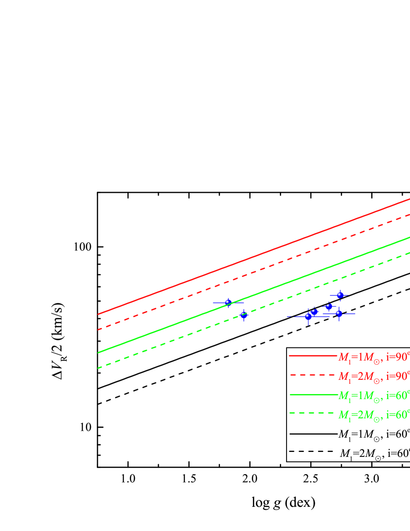
Figure 1: Comparison of the observations (blue circles) with the theoretical results (lines) in the $\Delta V_{R}/2-\log g$ diagram, where $M_{2}=3M_{\sun}$ is adopted for the theoretical calculations.

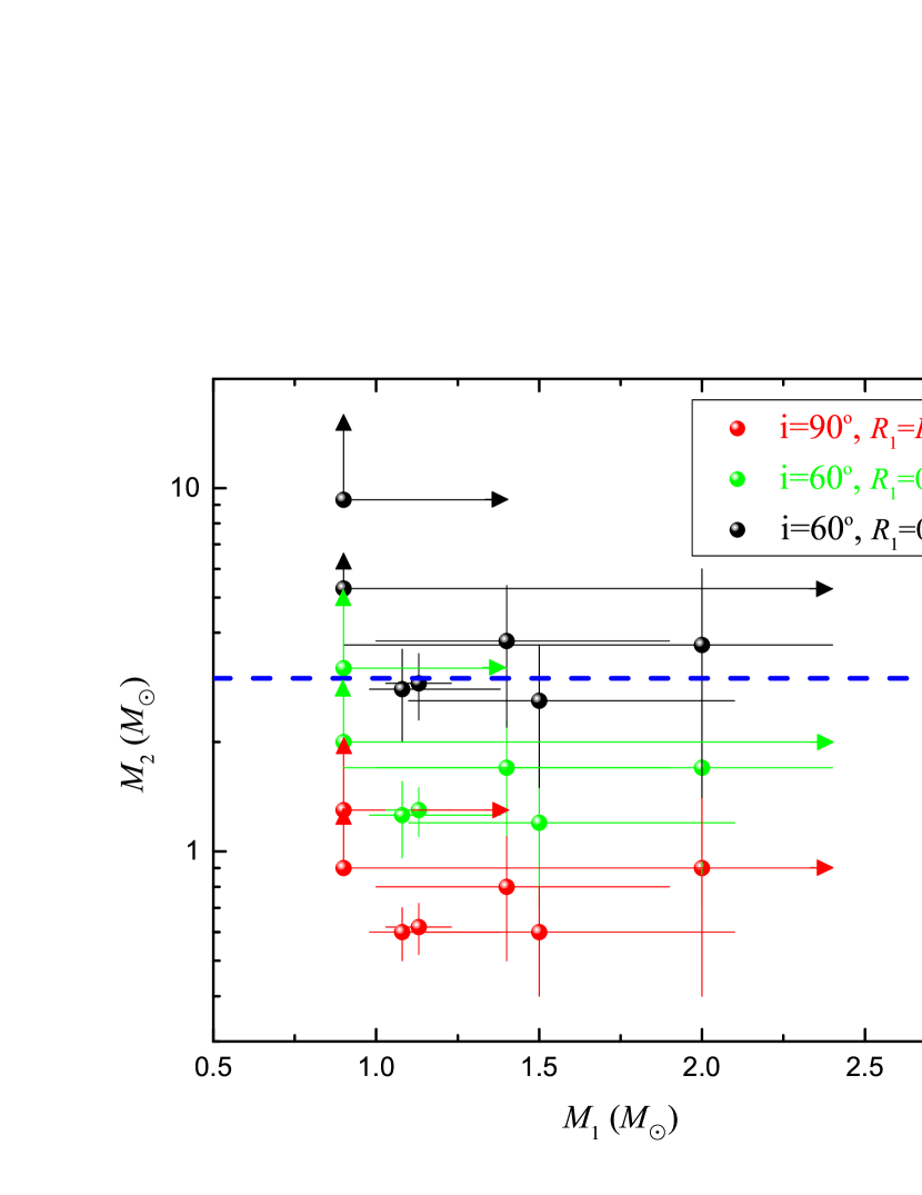
Figure 2: Evaluation of $M_{2}$ for the seven sources in our sample based on Equation (6), where three pairs of ($i$, $\lambda$) are adopted. The blue dashed line represents the critical mass $M_{2}=3M_{\sun}$.

Table 1: Parameters for the sources in our sample.

No.	RA	DEC	UCAC4	Vmag	$T_{\rm eff}$	$\log g$	$\rm[Fe/H]$	$N_{\rm obs}$	$\Delta V_{R}$	$\varpi$	$R_{1}^{\rm G}$	$R_{1}^{\rm LT}$
				(mag)	($\rm K$)	($\rm dex$)	($\rm dex$)		($\rm km~{}s^{-1}$)	($\rm mas$)	($R_{\sun}$)	($R_{\sun}$)
(1)	(2)	(3)	(4)	(5)	(6)	(7)	(8)	(9)	(10)	(11)	(12)	(13)
1	0.839246	38.518578	643-000232	12.736 $\pm$ 0.05	4696 $\pm$ 36	2.65 $\pm$ 0.06	-0.25 $\pm$ 0.03	3	93.5 $\pm$ 5.6	0.505 $\pm$ 0.043	9.15	10.8 $\pm$ 0.2
2	3.887134	38.688854	644-000944	12.665 $\pm$ 0.09	4301 $\pm$ 22	1.95 $\pm$ 0.04	-0.47 $\pm$ 0.02	4	83.7 $\pm$ 6.2	0.379 $\pm$ 0.032	15.82	19.7 $\pm$ 0.3
3	58.561194	45.43539	678-024276	15.054 $\pm$ 0.03	4943 $\pm$ 108	2.48 $\pm$ 0.17	-0.65 $\pm$ 0.10	3	81.9 $\pm$ 9.0	0.148 $\pm$ 0.034	–	14.7 $\pm$ 0.7
4	74.0532211	54.0059047	721-037069	12.784 $\pm$ 0.11	4823 $\pm$ 53	2.74 $\pm$ 0.08	-0.29 $\pm$ 0.05	4	107.5 $\pm$ 7.4	1.068 $\pm$ 0.034	6.34	7.0 $\pm$ 0.2
5	106.45855	13.606334	519-037128	14.51 $\pm$ 0.02	4655 $\pm$ 21	2.53 $\pm$ 0.03	-0.31 $\pm$ 0.02	3	87.5 $\pm$ 5.3	0.122 $\pm$ 0.030	–	18.4 $\pm$ 0.2
6	111.33637	28.067468	591-041200	14.698 $\pm$ 0.07	4832 $\pm$ 83	2.73 $\pm$ 0.13	-0.23 $\pm$ 0.08	6	85.1 $\pm$ 7.6	0.152 $\pm$ 0.032	–	11.9 $\pm$ 0.4
7	169.1288227	55.7284139	729-048720	10.638 $\pm$ 0.17	4191 $\pm$ 80	1.82 $\pm$ 0.12	-0.75 $\pm$ 0.07	3	97.8 $\pm$ 5.8	1.086 $\pm$ 0.031	13.14	17.9 $\pm$ 0.7

Note. — Column (1): Number of the source. Column (2): Right ascension (J2000). Column (3): Declination (J2000). Column (4): UCAC4 recommended identifier. Column (5): V-band magnitude from UCAC4. Column (6): Effective temperature from LDR6. Column (7): Surface gravity from LDR6. Column (8): Metallicity from LDR6. Column (9): Times of observations. Column (10): Observed largest variation of radial velocity. Column (11): Absolute stellar parallax from GDR2. Column (12): Radius of the giant star from GDR2. Column (13): Radius of the giant star based on the relation of the bolometric luminosity and the effective temperature.

Table 2: Evaluation of $M_{2}$ for the sources in our sample.

No.	Age	$M_{1}$	$R_{1}$	$M_{2}^{\rm I}$	$M_{2}^{\rm II}$	$M_{2}^{\rm III}$
	($10^{9}{\rm yr}$)	($M_{\sun}$)	($R_{\sun}$)	($M_{\sun}$)	($M_{\sun}$)	($M_{\sun}$)
(1)	(2)	(3)	(4)	(5)	(6)	(7)
1	$7.3^{+4.7}_{-3.8}$	$1.1^{+0.3}_{-0.1}$	$8.1^{+1.5}_{-0.8}$	0.6 $\pm$ 0.1	1.3 $\pm$ 0.3	2.9 $\pm$ 0.8
$2^{{{\dagger}}}$	$13^{+2.2}_{-0.1}$	$0.9^{+1.5}_{-}$	$17.8^{+0.6}_{-}$	$0.9^{+0.4}_{-}$	$2.0^{+0.7}_{-}$	$5.3^{+0.7}_{-}$
3	$0.97^{+9.64}_{-0.33}$	$2.0^{+0.4}_{-1.1}$	$13.3^{+2.7}_{-3.7}$	0.9 $\pm$ 0.5	1.7 $\pm$ 1.0	3.7 $\pm$ 2.3
4	$3.2^{+7.6}_{-1.9}$	$1.4^{+0.5}_{-0.4}$	$8.2^{+2.2}_{-1.7}$	0.8 $\pm$ 0.3	1.7 $\pm$ 0.6	3.8 $\pm$ 1.6
5	$6.3^{+3.1}_{-1.9}$	$1.1^{+0.1}_{-0.1}$	$9.5^{+0.8}_{-0.6}$	0.6 $\pm$ 0.1	1.3 $\pm$ 0.2	2.9 $\pm$ 0.6
6	$2.6^{+4.4}_{-1.6}$	$1.5^{+0.6}_{-0.4}$	$8.7^{+2.8}_{-1.9}$	0.6 $\pm$ 0.2	1.2 $\pm$ 0.5	2.6 $\pm$ 1.1
$7^{{{\dagger}}}$	$11^{+1}_{-9}$	$0.9^{+0.5}_{-}$	$20.8^{+8.1}_{-}$	$1.3^{+0.7}_{-}$	$3.2^{+1.8}_{-}$	$9.3^{+5.2}_{-}$

Note. — ^† The parameters of the second and the seventh sources cannot be well constrained, where $M_{1}=0.9M_{\sun}$ itself is the lower bound according to the PARSEC model. Column (1): Number of the source. Column (2): Age of the giant star from the PARSEC model. Column (3): Mass of the giant star from the PARSEC model. Column (4): Radius of the giant star from the PARSEC model. All the errors about the PARSEC model are 90% confidence. Column (5): Mass of $M_{2}$ for “$i=90^{\circ}$, $\lambda=1$”. Column (6): Mass of $M_{2}$ for “$i=60^{\circ}$, $\lambda=0.5$”. Column (7): Mass of $M_{2}$ for “$i=60^{\circ}$, $\lambda=0.2$”.

References

- Bolton (1972) Bolton, C. T. 1972, Nature, 235, 271
- Breivik et al. (2017) Breivik, K., Chatterjee, S., & Larson, S. L. 2017, ApJ, 850, L13
- Brown & Bethe (1994) Brown, G. E., & Bethe, H. A. 1994, ApJ, 423, 659
- Casares & Jonker (2014) Casares, J., & Jonker, P. G. 2014, Space Sci. Rev., 183, 223
- Corral-Santana et al. (2016) Corral-Santana, J. M., Casares, J., Muñoz-Darias, T., et al. 2016, A&A, 587, A61
- Cui et al. (2012) Cui, X.-Q., Zhao, Y.-H., Chu, Y.-Q., et al. 2012, Research in Astronomy and Astrophysics, 12, 1197
- Drake et al. (2014) Drake, A. J., Graham, M. J., Djorgovski, S. G., et al. 2014, ApJS, 213, 9
- Duemmler et al. (1997) Duemmler, R., Ilyin, I. V., & Tuominen, I. 1997, A&AS, 123, 209
- Eggleton (1983) Eggleton, P. P. 1983, ApJ, 268, 368
- Fitzpatrick (1999) Fitzpatrick, E. L. 1999, PASP, 111, 63
- Gaia Collaboration et al. (2018) Gaia Collaboration, Brown, A. G. A., Vallenari, A., et al. 2018, A&A, 616, A1
- Giesers et al. (2018) Giesers, B., Dreizler, S., Husser, T.-O., et al. 2018, MNRAS, 475, L15
- Green et al. (2018) Green, G. M., Schlafly, E. F., Finkbeiner, D., et al. 2018, MNRAS, 478, 651
- Guseinov & Zel’dovich (1966) Guseinov, O. K., & Zel’dovich, Y. B. 1966, Soviet Ast., 10, 251
- Høg et al. (2000) Høg, E., Fabricius, C., Makarov, V. V., et al. 2000, A&A, 355, L27
- Liu et al. (2014) Liu, C., Deng, L.-C., Carlin, J. L., et al. 2014, ApJ, 790, 110
- Liu et al. (2015) Liu, C., Fang, M., Wu, Y., et al. 2015, ApJ, 807, 4
- Luo et al. (2015) Luo, A.-L., Zhao, Y.-H., Zhao, G., et al. 2015, Research in Astronomy and Astrophysics, 15, 1095
- Marsh et al. (1994) Marsh, T. R., Robinson, E. L., & Wood, J. H. 1994, MNRAS, 266, 137
- Mashian & Loeb (2017) Mashian, N., & Loeb, A. 2017, MNRAS, 470, 2611
- Masuda & Hotokezaka (2018) Masuda, K., & Hotokezaka, K. 2018, arXiv:1808.10856
- Mazeh & Goldberg (1992) Mazeh, T., & Goldberg, D. 1992, ApJ, 394, 592
- Minniti et al. (2015) Minniti, D., Contreras Ramos, R., Alonso-García, J., et al. 2015, ApJ, 810, L20
- Moe & Di Stefano (2017) Moe, M., & Di Stefano, R. 2017, ApJS, 230, 15
- Paczyński (1971) Paczyński, B. 1971, ARA&A, 9, 183
- Remillard & McClintock (2006) Remillard, R. A., & McClintock, J. E. 2006, ARA&A, 44, 49
- Su & Cui (2004) Su, D.-Q., & Cui, X.-Q. 2004, Chinese J. Astron. Astrophys., 4, 1
- Thompson et al. (2018) Thompson, T. A., Kochanek, C. S., Stanek, K. Z., et al. 2018, arXiv:1806.02751
- Timmes et al. (1996) Timmes, F. X., Woosley, S. E., & Weaver, T. A. 1996, ApJ, 457, 834
- Torres (2010) Torres, G. 2010, AJ, 140, 1158
- Trimble & Thorne (1969) Trimble, V. L., & Thorne, K. S. 1969, ApJ, 156, 1013
- Voges et al. (2000) Voges, W., Aschenbach, B., Boller, T., et al. 2000, IAU Circ., 7432, 1
- Wang et al. (1996) Wang, S.-G., Su, D.-Q., Chu, Y.-Q., Cui, X., & Wang, Y.-N. 1996, Appl. Opt., 35, 5155
- Webster & Murdin (1972) Webster, B. L., & Murdin, P. 1972, Nature, 235, 37
- Wyrzykowski et al. (2016) Wyrzykowski, L., Kostrzewa-Rutkowska, Z., Skowron, J., et al. 2016, MNRAS, 458, 3012
- Yalinewich et al. (2018) Yalinewich, A., Beniamini, P., Hotokezaka, K., & Zhu, W. 2018, MNRAS, 481, 930
- Yamaguchi et al. (2018) Yamaguchi, M. S., Kawanaka, N., Bulik, T., & Piran, T. 2018, ApJ, 861, 21
- Zacharias et al. (2012) Zacharias, N., Finch, C. T., Girard, T. M., et al. 2012, VizieR Online Data Catalog, 1322