kiloparsec-scale Variations in the Star Formation Efficiency of Dense Gas: the Antennae Galaxies (NGC 4038/39)

Abstract

We study the relationship between dense gas and star formation in the Antennae galaxies by comparing ALMA observations of dense gas tracers (HCN, HCO⁺, and HNC $\mathrm{J}=1-0$) to the total infrared luminosity ($\mathrm{L_{TIR}}$) calculated using data from the Herschel Space Observatory and the Spitzer Space Telescope. We compare the luminosities of our SFR and gas tracers using aperture photometry and employing two methods for defining apertures. We taper the ALMA dataset to match the resolution of our $\mathrm{L_{TIR}}$ maps and present new detections of dense gas emission from complexes in the overlap and western arm regions. Using OVRO CO $\mathrm{J}=1-0$ data, we compare with the total molecular gas content, $\mathrm{M(H_{2})_{tot}}$, and calculate star formation efficiencies and dense gas mass fractions for these different regions. We derive HCN, HCO⁺ and HNC upper limits for apertures where emission was not significantly detected, as we expect emission from dense gas should be present in most star-forming regions. The Antennae extends the linear $\mathrm{L_{TIR}-L_{HCN}}$ relationship found in previous studies. The $\mathrm{L_{TIR}-L_{HCN}}$ ratio varies by up to a factor of $\sim$10 across different regions of the Antennae implying variations in the star formation efficiency of dense gas, with the nuclei, NGC 4038 and NGC 4039, showing the lowest SFE_dense (0.44 and 0.70 $\times 10^{-8}$ yr^-1). The nuclei also exhibit the highest dense gas fractions ($\sim 9.1\%$ and $\sim 7.9\%$).

1. Introduction

The Antennae galaxies are the nearest pair of merging galaxies (22 Mpc, Schweizer et al. 2008) and are rich in star formation (e.g. Whitmore et al. 1999), gas (e.g. Wilson et al. 2000, 2003), and dust (e.g. Klaas et al. 2010). The rarity of wet, major mergers (gas-rich galaxies with a mass ratio $\leq$ 3) makes the Antennae a particularly unique environment for studying star formation in interactions. Recent simulations suggest the Antennae is $\sim 40$ Myr after its second pass (Karl et al., 2010), placing it at an intermediate stage in the Toomre sequence. Thus, the Antennae contains multiple generations of stars from merger-induced starburst behavior. The two nuclei exhibit post-starburst populations $\sim$65 Myr old (Mengel et al., 2005), and even younger starburst populations ($\sim 3-10$ Myr) are concentrated in the overlap region and western arm (e.g. Mengel et al. 2001, 2005; Whitmore et al. 2010, 2014). Furthermore, different regions within the Antennae exhibit varying degrees of current ($\leq 100$ Myr, Brandl et al. 2009) star formation, with the overlap region of the Antennae (see Fig. 1) experiencing a particularly violent episode ( Star Formation Rate, SFR $>4$ M_⊙ yr^-1, Brandl et al. 2009; Klaas et al. 2010; this work).

Major mergers are a testbed for the extreme star formation ongoing at high-z, and show fundamental differences in their star formation properties compared with normal star-forming disk galaxies (e.g. Daddi et al. 2010; Tacconi et al. 2018). Futhermore, star formation occurs primarily in the densest regions within Giant Molecular Clouds (GMCs, $\mathrm{n(H_{2})}>10^{4}$ cm^-3 , Lada et al. 1991a, b). The HCN $\mathrm{J}=1-0$ transition has a critical density of $\mathrm{n_{crit}}\sim 10^{5}$ cm^-3, while the CO $\mathrm{J}=1-0$ has $\mathrm{n_{crit}}\sim 10^{2}$ cm^-3. Thus, it is essential to observe molecules such as HCN to constrain the properties of the directly star-forming gas.

Extragalactic studies often use observations of the total infrared luminosity ($\mathrm{L_{IR}}$) and HCN J$=1-0$ molecular luminosity ($\mathrm{L_{HCN}}$) in galaxies to study star formation and dense gas. This has largely been motivated by the seminal work of Gao & Solomon (2004a, b), who found a tight and linear relationship between the global values of $\mathrm{L_{IR}}$ and $\mathrm{L_{HCN}}$ in a sample of 65 galaxies. Their observations were of unresolved systems, thus comparing the Total Infrared (TIR) and HCN luminosities spanning $\mathrm{L_{IR}}\sim 10^{9}-10^{12}$ L_⊙. This sample included normal star-forming galaxies as well as more extreme Luminous and Ultraluminous Infrared Galaxies (LIRGs/ULIRGs), suggesting a direct scaling between the SFR and dense molecular gas content across galaxy types. Other recent studies show that this linear relationship also extends to the scales of individual, massive clumps in the Milky Way and nearby galaxies (e.g. Wu et al. 2005, 2010; Bigiel et al. 2015; Chen et al. 2015), spanning nearly 10 orders of magnitude in luminosity. These observations have motivated density-threshold models of star formation (Lada et al., 2012), which assume that star formation begins once the gas reaches a threshold density ($\mathrm{n(H_{2})}=10^{4}$ cm^-3). These models predict a constant Star Formation Efficiency of dense gas (SFE_dense) that should span all regimes of star formation.

A number of recent studies target the $\mathrm{L_{TIR}-L_{\mathrm{HCN}}}$ relationship on a variety of scales, down to several hundred parsecs (Kepley et al., 2014; Bigiel et al., 2016; Gallagher et al., 2018). These studies fit well within the scatter of the original Gao & Solomon (2004a, b) relationship, extending it down to lower luminosities. Some have also revealed variations in the $\mathrm{L_{IR}}$ and $\mathrm{L_{HCN}}$ relationship at $\sim$kpc scales (e.g. M51 from Chen et al. 2015; Usero et al. 2015). Usero et al. (2015) study $\sim$kpc scales across the disks of normal star-forming galaxies and find a sublinear power-law index ($\sim 0.5$) for their sample of galaxies. Furthermore, evidence exists that (U)LIRGs may turn off the linear portion of the $\mathrm{L_{IR}-L_{HCN}}$ sequence (Graciá-Carpio et al., 2008), suggesting variations at the high luminosity end as well.

A separate class of star formation models that can, to some degree, better explain the variations of the $\mathrm{L_{IR}-L_{HCN}}$ relationship are turbulence-regulated density threshold models (Krumholz & McKee, 2005; Padoan & Nordlund, 2011). These models predict the variation of probability density profiles (PDFs) as a function of turbulence, and show that turbulence acts as a star formation inhibitor and subsequently increases the threshold density of gas required for star formation. Observational evidence of a correlation between stellar mass density and lower $\mathrm{L}_{\mathrm{TIR}}/\mathrm{L}_{\mathrm{HCN}}$ in disk galaxies supports the idea that stellar feedback, in the form of turbulence, etc., can inhibit star formation per unit dense gas mass (Bigiel et al., 2016). Interestingly, there have been observations of increases in the dense gas fraction (often traced by $\mathrm{L}^{{}^{\prime}}_{\mathrm{HCN}}/\mathrm{L}^{{}^{\prime}}_{\mathrm{CO}}$) in the central regions of disk galaxies, where the star formation efficiency of dense gas (traced by $\mathrm{L}_{\mathrm{TIR}}/\mathrm{L}^{{}^{\prime}}_{\mathrm{HCN}}$) appears lowest and stellar density appears highest. The Central Molecular Zone (CMZ) of the Milky Way is the closest example of an environment with low SFE_dense and high dense gas fractions (e.g. Kauffmann et al. 2017b, c) compared to the solar neighborhood. There are a number of possible mechanisms that can explain this, with turbulence being the favored mechanism so far (Federrath & Klessen, 2012; Kruijssen et al., 2014; Rathborne et al., 2014). Federrath & Klessen (2012) compare the expectations of six different star formation with Magnetohydrodynamic (MHD) simulations that vary four fundamental parameters: virial parameter, sonic mach number, turbulent forcing parameter, and Alfven mach number. They find turbulence is the primary regulator of the SFR, and produce star formation efficiencies of the total gas (SFE) that agree well with observations ($1-10\%$).

High-resolution Atacama Large Millimeter/submillimeter Array (ALMA) observations have revealed HCN, HCO⁺, and HNC $\mathrm{J}=1-0$ emission throughout star-forming regions in the Antennae (Schirm et al., 2016). Assuming these transitions trace $\mathrm{n(H_{2})}>10^{4}$ cm^-3, this suggests there is an abundance of dense gas throughout this system. Futhermore, there are interesting variations in the molecular luminosities of these dense gas tracers, suggesting differences in dense gas properties across the system. Schirm et al. (2016) found evidence for variations of the dense gas fraction across the Antennae, evidenced by higher HCN-to-CO luminosity ratios in the two nuclei when compared to the overlap region (see Fig. 1). Bigiel et al. (2015) find that the $\mathrm{L_{IR}-L_{HCN}}$ relationship in the brightest regions of the Antennae galaxies is consistent with the linear relationship revealed by Gao & Solomon (2004a, b), but their sensitivity limits miss a large portion of the star-forming regions in the system (e.g. the western arm and fainter regions in the overlap region). In this paper, we attempt to understand the variations of this relationship in the context of the Antennae galaxies by assessing the variations of the physical properties with $\mathrm{L}_{\mathrm{TIR}}-\mathrm{L}^{{}^{\prime}}_{\mathrm{HCN(1-0)}}$ at subgalactic scales.

In §2, we present the ALMA, Herschel, and Spitzer data used in our study along with the total infrared luminosity calibrations. In §3, we describe our aperture photometry analyses. In §4, we present the luminosity fit results and compare to previous work. In §5, we discuss the variation we see in $\mathrm{SFE_{dense}}$ across the Antennae and explore potential explanations for these variations. The analysis and results of this study are summarized in §6. Molecular and infrared luminosity uncertainties are discussed in more detail in Appendix A. A comparison between total infrared luminosity calbrations from Galametz et al. (2013) is presented in Appendix B.

2. Data

We use Herschel, Spitzer, and ALMA data in our study to compare star formation traced by infrared emission to dense gas traced by high critical-density molecular transitions, HCN, HCO⁺, and HNC $\mathrm{J}=1-0$ (see Figure 1). We also use CO $\mathrm{J}=1-0$ data from the Owens Valley Radio Observatory (OVRO, Wilson et al. 2003) as our bulk molecular gas tracer, and we note that the OVRO data may be missing $\sim 20\%$ of the CO $\mathrm{J}=1-0$ flux (Schirm et al., 2016), likely a diffuse component of the gas, due to the limited range of $u-v$ coverage. Our resolution is limited by the Herschel data ($5.5^{\prime\prime}$ at 70 $\mu$m, and $6.8^{\prime\prime}$ at 100 $\mu$m), and thus our analysis is performed at these resolutions.

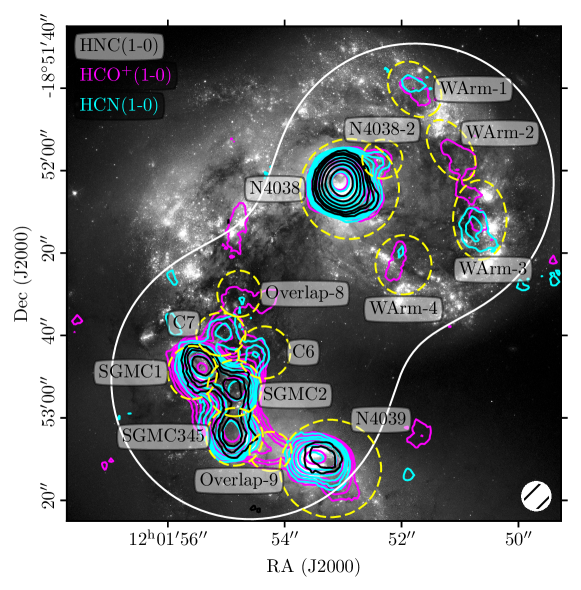
Figure 1.— Magenta, cyan, and black contours (levels = $0.06\times$[4, 6, 8, 12, 17, 24, 34, 49, 70, 100] Jy beam^-1 km s^-1) of the ALMA HCO⁺, HCN, and HNC J$=1-0$ transitions, respectively, overlaid on top of a black and white composite image (435 nm, 550 nm, and 658 nm) from HST. The elliptical apertures are outlined with yellow, dashed curves and labeled according to Tables 3 and LABEL:tab:ell_lumin; the 50$\%$ ALMA primary beam sensitivity is shown as the solid, white curve. The smoothed beam size ($6.8^{\prime\prime}$) of the ALMA data is shown in the lower right.

2.1. ALMA Data

Details on the observations of the ALMA data are available in Schirm et al. (2016). The original reduction scripts were used to apply calibrations to the raw data using the appropriate Common Astronomy Software Applications (CASA) version (CASA 4.2.0, McMullin et al. 2007). The ALMA data were then cleaned and imaged in in CASA 4.7.2. We cleaned using a velocity resolution of $\Delta\mathrm{v_{opt}}=5.2\ \mathrm{km\ s}^{-1}$ at the rest frequency of each transition over an optical velocity range of 1000-2000 km s^-1. We tapered the data to the Full-Width Half-Maximum (FWHM) of the Herschel 70 $\mu$m Point Spread Function using a Briggs weighting of $0.5$ while cleaning. The largest angular scale of the ALMA observations is $\sim 17^{\prime\prime}$ ($\sim 1.8$ kpc). The tapered data reach a root mean square noise level (rms) of $\sigma=1.2\ \mathrm{mJy\ beam}^{-1}$. When working at the $100\ \mu$m resolution, we further smooth the tapered cube to $6.8^{\prime\prime}$.

We create moment zero maps of the molecular lines using CASA’s immoments command. This produces a two-dimensional image of the integrated intensity with units of Jy beam^-1 km s^-1. We require that all pixels going into the final moment map be greater than $2\sigma$, where $\sigma=1.2$ mJy beam^-1 in the $5.5^{\prime\prime}$ maps and $\sigma=1.4$ mJy beam^-1 in the smoothed 6.8^′′ maps. We then convert to molecular luminosities ($\mathrm{L^{\prime}_{mol}}$) using the following equation (Wilson et al., 2008)

$$\frac{\mathrm{L^{\prime}_{mol}}}{\textrm{K km s}^{-1}\ \textrm{pc}^{2}} =3.2546\times 10^{7}\left(\frac{\mathrm{S_{ap}}}{\textrm{Jy km s}^{-1}}\right)\times$$

$$\qquad\left(\frac{\mathrm{D_{L}}}{\textrm{Mpc}}\right)^{2}\left(\frac{\nu_{0}}{\textrm{GHz}}\right)^{-2}(1+\mathrm{z})^{-1}$$ (1)

where $\mathrm{S_{ap}}$ is the flux measured in an aperture in $\textrm{Jy km s}^{-1}$. This gives molecular luminosity in units of $\textrm{K km s}^{-1}\textrm{ pc}^{2}$. We use a redshift of $\mathrm{z}=0.005477$. Details on the uncertainty estimates are given in §3 and Appendix A.I.

2.2. Infrared Data and Total Infrared Luminosities

We obtain user-provided data products of the 70, 100, 160, and 250 $\mu$m maps from the Herschel (Pilbratt et al., 2010) Science Archive. Details on the observations and reduction of the 70, 100, and 160 $\mu$m (Photodetector Array Camera and Spectrometer) PACS (Poglitsch et al., 2010) data are available in Klaas et al. (2010) and reach resolutions of $5.5^{\prime\prime}$, $6.8^{\prime\prime}$, and $11.3^{\prime\prime}$, respectively. The Spectral and Photometric Imaging Receiver (SPIRE) 250 $\mu$m map ($18.1^{\prime\prime}$ resolution, Griffin et al. 2010) was obtained as part of the Very Nearby Galaxies Survey and details on the observations and calibrations can be found in Bendo et al. (2012b). We also retrieve user-provided Spitzer (Werner et al., 2004) 24 $\mu$m Multiband Imaging Photometer (MIPS) data (Rieke et al. 2004, $6.0^{\prime\prime}$ resolution) from the Spitzer Heritage Archive. These data were reprocessed by Bendo et al. (2012a) to provide ancillary data for the Herschel-SPIRE Local Galaxies Guaranteed Time Programs.

We use several calibrations from Galametz et al. (2013) to estimate L_TIR, which is defined in that paper to be:

$$\mathrm{L_{TIR}}=\int_{3\ \mu\mathrm{m}}^{1100\ \mu\mathrm{m}}\mathrm{L}_{\nu}\mathrm{d}\nu.$$

Galametz et al. (2013) derive calibrations of L_TIR using a combination of Herschel and Spitzer data from $8-250\ \mu\mathrm{m}$ as an alternative to fitting the dust spectral energy distribution (SED). They have provided monochromatic calibrations (e.g. 70 $\mu$m), as well as multi-band calibrations (e.g. 24+70+100 $\mu$m). We compare several of these calibrations for the Antennae in Appendix B and show the ratio maps for these calibrations in Figure 6 at the 250 $\mu$m resolution ($18.1^{\prime\prime}$).

In this paper, we use the monochromatic 70 $\mu$m (5.5” $\sim$ 590 pc) and the multi-band $24+70+100\ \mu$m (6.8” $\sim$ 725 pc) calibrations to estimate L_TIR across the Antennae. The 70 $\mu$m calibration is the highest-resolution Herschel band and brackets the warm-dust (30-60 K) Spectral Energy Distribution (SED) peak ($\sim 100\ \mu$m). For multi-band calibrations, Galametz et al. (2013) recommend that any L_TIR estimate using less than 4-5 bands should include the 100 $\mu$m flux or a combination of the $70+160$ bands, which should lead to L_TIR predictions reliable within 25% ($\leq 50\%$ for monochromatic calibrations). Additionally, Galametz et al. (2013) note that including the 24 $\mu$m flux improves calibrations of L_TIR for galaxies with higher 70/100 color, i.e. strongly star-forming environments. The overlap region is known to be vigorously star-forming, which could cause the 70 $\mu$m flux to underestimate L_TIR. Therefore, we include the $24+70+100\ \mu$m calibration as a check for this. Overall, we find our L${}_{\mathrm{TIR}}(70)$ estimates agree well with the L${}_{\mathrm{TIR}}(24+70+100)$ estimates. The L${}_{\mathrm{TIR}}(70)$ estimate for SGMC345 (the combination of SGMCs 3, 4, and 5 from Wilson et al. 2000) is only $\sim 3\%$ lower than the L${}_{\mathrm{TIR}}(24+70+100)$ estimate and agrees within uncertainties.

To estimate L_TIR using multiple IR bands, we converted the Herschel and Spitzer maps to the same units and resolution (i.e. to the FWHM of the beam size of the band with the lowest resolution). The Spitzer MIPS and Herschel SPIRE data were converted to units of Jy pixel^-1 from MJy sr^-1 and Jy beam^-1, respectively (the Herschel PACS data were already in units of Jy pixel^-1). Each dataset was then convolved to a common resolution using the Aniano et al. (2011) kernels. The Galametz et al. (2013) calibrations require infrared measurements be in solar luminosity units ($\text{L}_{\odot}$). We convert the Herschel infrared maps from Jansky units to solar luminosities using the following equation

$$\frac{\nu\mathrm{L}_{\nu}}{\mathrm{L_{\odot}}}=3.1256\times 10^{2}\left(\frac{\mathrm{d_{L}}}{\mathrm{Mpc}}\right)^{2}\left(\frac{\nu}{\mathrm{GHz}}\right)\left(\frac{\mathrm{S}_{\nu}}{\mathrm{Jy}}\right).$$ (2)

The background is then estimated and subtracted from each map. Once the data are formatted properly, we apply the corresponding Galametz et al. (2013) calibrations to create L_TIR maps. We calculate absolute uncertainties on the L_TIR calibrations (see Appendix A.II for details) and find they are much lower than the calibration uncertainties quoted above (25$\%$ uncertainties on the L${}_{\mathrm{TIR}}(24+70+100)$ measurements and $\sim 50\%$ uncertainties on the L_TIR(70) measurements).

3. Aperture Analysis

We compare the emission of our SFR and gas tracers across different regions of the Antennae using aperture photometry. We use two approaches to defining apertures. In our first method, we identify clumps of emission using cprops (Rosolowsky & Leroy, 2006) in each of the dense gas data-cubes; we then manually define elliptical apertures (Table 3) to encompass infrared and integrated intensity dense-gas emission of individual “clumps” or complexes. We vary the radii and position angles of the apertures to encompass potentially-associated emission of the IR and dense-gas tracers. In our second method, we perform a “pixel-by-pixel” analysis by dividing the maps into hexagonal grids that are sampled by the FWHM of the beam (i.e. the incircle diameter of each hexagon is $6.8^{\prime\prime}$). The hexagons are fixed in size across the map (edge = $3.9^{\prime\prime}$; inspired by a similar method employed by Leroy et al. 2016). The elliptical aperture method allows us to contrast the behavior of individual regions, while the hexagonal method eliminates selection bias that can be introduced in the manual-aperture method. Therefore, the hexagonal aperture method provides more robust data for trend-fitting, and the emphasis of the elliptical aperture analysis is region-by-region comparisons.

Table 1Elliptical Apertures

Source	RA	Dec	EW	NS	Area
	(J2000)	(J2000)	(′′)	(′′)	(kpc2)
NGC4038	$12:01:52.895$	$-18:52:04.46$	24.1	24.3	5.23
NGC4039	$12:01:53.22$	$-18:53:12.29$	24.6	23.7	5.22
NGC4038-2	$12:01:52.332$	$-18:51:57.2$	9.8	9.5	0.84
WArm-1	$12:01:51.779$	$-18:51:40.27$	11.4	14.9	1.52
WArm-2	$12:01:51.156$	$-18:51:55.04$	9.5	16.3	1.39
WArm-3	$12:01:50.664$	$-18:52:11.98$	13.0	19.3	2.26
WArm-4	$12:01:51.97$	$-18:52:22.86$	13.6	14.4	1.76
SGMC1	$12:01:55.583$	$-18:52:49.02$	12.0	12.9	1.38
SGMC2	$12:01:54.862$	$-18:52:52.8$	13.1	13.7	1.60
SGMC345	$12:01:54.862$	$-18:53:04.6$	13.8	14.0	1.73
Schirm-C6	$12:01:54.351$	$-18:52:44.13$	12.6	12.7	1.44
Schirm-C7	$12:01:55.094$	$-18:52:39.71$	12.0	10.5	1.12
Overlap-8	$12:01:54.781$	$-18:52:29.88$	10.6	11.2	1.05
Overlap-9	$12:01:54.246$	$-18:53:08.14$	10.2	9.5	0.86

• Note. – The center coordinates and angular extent of the elliptical apertures. The axes are oriented East-West (EW) and North-South (NS) except for WArm-1, WArm-2, and WArm-3 where the position angles (PA) are 42.2^∘, 32.3^∘, and 1.3^∘ east of north.

We perform the luminosity-luminosity fits using the Bayesian linear regression code linmix (Kelly, 2007), which incorporates uncertainties in both x- and y-directions. The linmix routine assumes a linear relationship of the form $\mathrm{log(L_{TIR})=m\times log(L_{dense})+log(b)}$, where m is the slope, and b is the y-intercept. The linmix code also allows us to incorporate upper limits into our fits, therefore we also include upper limits of the molecular luminosities in the fits. We estimate the significance of each correlation by calculating the Spearman rank coefficients of the datasets for each fitted relationship. The one- and two-sigma uncertainties on the fits are estimated via Markov-Chain Monte-Carlo (MCMC), and we take the median values of these iterations as our fit parameters. We compare our results with those of Gao & Solomon (2004a, b) and Liu et al. (2015) and also perform fits of the Antennae data combined with datasets from these studies. We also compare with measurements of $\mathrm{L_{TIR}}$ and $\mathrm{L_{HCN}}$ of the CMZ (Stephens et al., 2016) since we observe similarities between luminosity ratios of the CMZ and the two nuclei (see §5.2.1). The HCN luminosity for the CMZ is derived from the Mopra CMZ 3mm survey, covering a $2.5^{\circ}\times 0.5^{\circ}$ area centered on $\mathit{l}=0.5^{\circ}$, $\mathit{b}=0.0^{\circ}$ (Jones et al., 2012), and the conversion to luminosity assumes a distance of 8.34$\pm$0.16 kpc (Reid et al., 2014). The infrared luminosity of the CMZ is estimated using a combination of 12, 25, 60, and 100 $\mu$m Infrared Astronomical Satellite (IRAS) fluxes and the calibration from Sanders & Mirabel (1996). We note that this region of the Milky Way is very crowded, and these luminosities are likely upper limits and may include emission from other sources along the line of sight. We assume uncertainties of $\sim 30\%$ on $\mathrm{L_{TIR}}$ and $\mathrm{L_{HCN}}$ of the CMZ since these are also the uncertainties prescribed by Liu et al. (2015) to the galaxies in their sample.

To determine upper limits of the Antennae luminosities, we first estimate the contribution of noise into each moment zero map. We approach this differently than applying a simple rms noise limit due to the large physical extent of the apertures (i.e. larger than the GMCs in our beam), and the large velocity range over which our moment maps are created. The moment zero maps are created with a two-sigma cutoff, such that no emission below two-sigma is allowed into the map. Since the noise follows a Gaussian distribution, only $\sim$2$\%$ of the noise should remain above this two-sigma cutoff; choosing a cutoff at two-sigma allows us to eliminate the majority of the noise from the moment zero map without sacrificing a significant amount of real emission. However, because $\sim$2$\%$ of the noise remains, each aperture will contain some signal from the noise proportional to the number of pixels per aperture ($\mathrm{n_{pix}}\simeq 117$ for the hexagonal apertures, and varies for the elliptical apertures) and the total number of channels in the datacube ($\mathrm{n_{chan}}=192$). Furthermore, the noise varies with position in the map according to the response of the primary beam ($\epsilon_{\mathrm{pb}}$). Optimally, the base rms noise is $\sigma=1.2$ mJy beam^-1 (5.5^′′) or $\sigma=1.4$ mJy beam^-1 (6.8^′′) at an efficiency of 100$\%$, and larger as the response decreases towards the edges of the primary beam.

Therefore, the remaining Gaussian noise per aperture in the moment zero maps, $\mathrm{\sigma^{ap}_{Gauss}}$, is

$$\mathrm{\sigma^{ap}_{Gauss}\approx 0.025\times\frac{2\sigma}{\epsilon_{pb}}\times\Delta v\times\mathrm{n_{pix}}\times\mathrm{n_{chan}}\div ppb}$$ (3)

where $\Delta\mathrm{v}=5.2$ km s^-1 and ppb is the number of pixels per beam (to give units of Jy km s^-1). We require the aperture sums from the moment zero maps of the dense gas tracers to be larger than this noise limit to be considered a detection. We set our upper limit to two times this noise limit:

$$\mathrm{\sigma^{ap}_{lim}} =2\times\mathrm{\sigma^{ap}_{Gauss}}$$ (4)

This requires at least $0.025\times 192=5$ channels (per pixel per aperture) to have a signal of four-sigma to be considered a detection. Anything below $\mathrm{\sigma^{ap}_{lim}}$ is considered an upper limit, and we set the values of these apertures to $\mathrm{\sigma^{ap}_{lim}}$ and treat them as upper limits in our fitting routines. The upper limits are shown as the gray arrows in Figure LABEL:fig:hex_pixels. At the 6.8^′′ resolution, the limit per hexagonal aperture is set to be $\mathrm{\sigma^{ap}_{lim}}\approx$ 110 mJy km s^-1 at maximum primary beam efficiency (which corresponds to 0.9 mJy km s^-1 per pixel), and translates to luminosity limits of $\mathrm{log(L_{HCN})}=5.46$, $\mathrm{log(L_{HCO^{+}})}=5.46$, and $\mathrm{log(L_{HNC})}=5.45$.

4. Results

Each approach to defining apertures has its own strengths: the hexagonal-grid approach allows us to optimally sample our datasets without introducing selection bias into our apertures, and the elliptical aperture analysis has the benefit of emphasizing individual source behavior. We therefore focus on the hexagonal aperture results when discussing fits, and then later focus on the results of the elliptical apertures when discussing variations in different regions of the Antennae.

In the tapered ALMA dataset, we detect significant emission from HCN and HCO⁺ in both the nuclei (NGC 4038 and NGC 4039), the overlap region (containing SGMCs 1-5, C6 and C7 from Schirm et al. 2016, and newly-detected sources 8 and 9), and the western arm (containing WArm 1-4). HNC is detected significantly in NGC 4038 and SGMCs in the overlap region, and upper limits are derived elsewhere. HCO⁺ is the overall brightest dense gas tracer in this dataset, and there are several regions where we detect HCO⁺ but not HCN; this includes the“bridge” region (Overlap-8) between SGMCs 3, 4, and 5 (hereafter referred to as one source, SGMC345) and NGC 4039 (the southern nucleus). HCO⁺ is also brightest in one of the regions we study in the western arm (WArm-2).

We plot the $\mathrm{L_{TIR}-L_{dense}}$ Antennae datapoints of the hexagonal and elliptical apertures in Figures LABEL:fig:hex_pixels and LABEL:fig:ell_results, respectively, and we list the luminosities measured within the elliptical apertures in Table LABEL:tab:ell_lumin. We overplot the linmix fits in grayscale (including upper limits) for both the hexagonal and elliptical aperture analyses; for comparison, we also plot fits to the hexagonal aperture luminosities without upper limits (salmon). The slopes and y-intercepts of the fits that includes upper limits are shown in each plot. We list the fits from the hexagonal apertures below. The $\mathrm{L_{TIR}-L_{dense}}$ fits present sub-linear power-law indices (i.e. $\mathrm{m}<1.0$). The Spearman p-values indicate strong correlations ($\mathrm{p}<0.05$) between $\mathrm{L_{TIR}}$ and the dense gas molecular luminosities, except for the HNC fits which shows a weaker correlation ($\mathrm{p}\sim 0.14$) likely due to the lower detection rate of this molecular line.

• Note. – Luminosities measured from the elliptical apertures listed in Table 3. All values are measured at the 100 $\mu$m resolution (6.8^′′). The absolute uncertainties are shown next to each luminosity, except in the case of limits.

• This $\mathrm{L_{TIR}}$ is estimated using the Galametz et al. (2013) calibration that combines the Spitzer 24 and Herschel 70 and 100 $\mu$m maps. See Table B for a comparison with Galametz et al. (2013) monochromatic 70 $\mu$m $\mathrm{L_{TIR}}$ estimates.

The fits from the hexagonal apertures shown in Figure LABEL:fig:hex_pixels are as follows:

$$\mathrm{log}(\mathrm{L_{TIR}}) =6.3^{+0.4}_{-0.5}+0.49^{+0.09}_{-0.08}\mathrm{log}(\mathrm{L_{HCN}})$$ (5)

$$\mathrm{log}(\mathrm{L_{TIR}}) =5.9^{+0.3}_{-0.4}+0.52^{+0.07}_{-0.06}\mathrm{log}(\mathrm{L_{HCO^{+}}})$$ (6)

$$\mathrm{log}(\mathrm{L_{TIR}}) =5.8^{+0.6}_{-0.9}+0.61^{+0.16}_{-0.11}\mathrm{log}(\mathrm{L_{HNC}})$$ (7)

We also fit the $\mathrm{L_{TIR}}$ and $\mathrm{L_{HCN}}$ values from the Antennae hexagonal apertures with those of the sources in Liu et al. (2015); Liu et al. (2015) includes the data from the Gao & Solomon (2004a, b) survey. This fit is presented in Figure 4. The power-law index on this fit is $\mathrm{m}=0.96\pm 0.03$, which is slightly sublinear. The Antennae data extend the datapoints of Gao & Solomon (2004a, b) and Liu et al. (2015) to lower luminosities. This agrees with the findings of Bigiel et al. (2015), who performed a similar analysis on the Antennae using data from the Combined Array for Research in Millimeter-wave Astronomy (CARMA). The median value of the $\mathrm{L_{TIR}/L_{HCN}}$ ratio of the Antennae hexagonal apertures (980 $\mathrm{L_{\odot}}$ (K km s^-1 pc²)^-1) falls within the scatter of other studies (i.e. Gao & Solomon 2004a, b; Liu et al. 2015). The scatter of the Antennae data is also comparable ($\sim$0.4 dex) to these other studies (Table LABEL:tab:stats). Fitting the surface densities of the Liu et al. (2015) and Antennae data also yields a slope $\mathrm{m=1}$ (Fig. 5).

• Note. – We calculate both Gaussian (mean, standard deviation) and non-Gaussian statistics (median, $16^{\mathrm{th}}$, and $84^{\mathrm{th}}$ percentiles), excluding upper limits. Quantities are in units of $\mathrm{L_{\odot}}$ (K km s^-1 pc²)^-1.

• Distance from the median to the $16^{\mathrm{th}}$ percentile.

• Distance from the median to the $84^{\mathrm{th}}$ percentile.

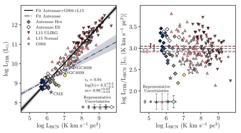
Figure 4.— Left: L_TIR vs. L_HCN datapoints of the Gao & Solomon (2004a, b) sample (gray circles), the Liu et al. (2015) (U)LIRGs (maroon inverted triangles), the Liu et al. (2015) normal star-forming galaxies (salmon triangles), the Antennae hexagonal aperture luminosities (blue-yellow diamonds), and the Antennae elliptical aperture luminosities (white diamonds). We emphasize the datapoints of the two nuclei, NGC 4038 and NGC 4039, as white stars. The hexagonal datapoints are colorized according to HCN luminosity as is done in Fig. LABEL:fig:hex_pixels. We show measurements of the CMZ (as given in Stephens et al. 2016) for comparison as the blue star (see text for more information). We show the fit to the Liu et al. (2015) and Antennae hexagonal data points (black solid line), with the one- (light shade) and two-sigma (dark shade) uncertainties from the MCMC iterations. The resulting fit parameters are listed (assuming $\mathrm{log(L_{TIR})=m\times log(L_{dense})+log(b)}$, where m is the slope, and b is the y-intercept). The fit to the Antennae hexagonal apertures from Fig. LABEL:fig:hex_pixels is shown for comparison as the dash-dot line in blue. Right: $\mathrm{L_{TIR}/L_{HCN}}$ vs. L_HCN. We show the median value (dashed line, see Table LABEL:tab:stats) of the $\mathrm{L_{TIR}/L_{HCN}}$ ratio for each dataset, excluding the Antennae elliptical apertures. At the left end of the dashed lines, we show the statistical uncertainties on the median values. We show representative uncertainties in the lower right corner (left plot) and lower left corner (right plot). Upper limits are excluded. The two nuclei have the lowest $\mathrm{L_{TIR}/L_{HCN}}$ in the Antennae system, despite having the highest dense gas fractions. The CMZ is also known to have a low star formation efficiency of dense gas and very high dense gas fractions.

• Note. – Estimates of physical properties from sources contained within the elliptical apertures (see Table 3). These properties are derived from the luminosities listed in Table LABEL:tab:ell_lumin. See §4 for further information about the conversion from luminosities to these values and the corresponding uncertainties.

We convert the total infrared luminosity to estimates of the star formation rates using the calibration initially published in Kennicutt (1998) and updated in Kennicutt & Evans (2012) with the more recent Kroupa initial mass function and Starburst99 model (Hao et al., 2011; Murphy et al., 2011)

$$\mathrm{log}\ \mathrm{SFR}\ (\mathrm{M_{\odot}\ yr}^{-1}) =\mathrm{log}\ \mathrm{\frac{L_{TIR}}{(L_{\odot})}}-9.83.$$ (8)

The uncertainty on the total infrared luminosities used for the SFR estimates is $\sim 25\%$ (Galametz et al., 2013) and thus we suggest this as a lower limit to the uncertainty on the SFRs derived via Eq. 8 and listed in Table LABEL:tab:ell_props.

We estimate the dense molecular gas content, $\mathrm{M_{dense}}$, from the HCN luminosities using the conversion factor published by Gao & Solomon (2004a), $\mathrm{\alpha_{HCN}}\ \approx 10\ \mathrm{M_{\odot}\ (K\ km\ s^{-1}\ pc^{2})^{-1}}$. We discuss the possibility of variations in the HCN conversion factor in §5.5. To estimate the total molecular gas content, $\mathrm{M_{H_{2}}}$, we adopt a CO-to-$\mathrm{H_{2}}$ conversion factor of $\mathrm{\alpha_{CO}}\ \approx 7\ \mathrm{M_{\odot}\ (K\ km\ s^{-1}\ pc^{2})^{-1}}$ from Schirm et al. (2014). Schirm et al. (2014) estimate the CO abundance and conversion factor in the Antennae by modelling a warm and cold gas component using RADEX (van der Tak et al., 2007) and Herschel Fourier Transform Spectrometer (FTS) data of multiple CO transitions. Using an initial CO abundance of $x_{\mathrm{CO}}\sim 3\times 10^{-4}$, they derive a warm H₂ gas mass that is $~{}10$ times lower than previous estimates from Brandl et al. (2009) based on direct H₂ observations; assuming CO is tracing the same gas as H₂, they adjust their CO abundance to $x\sim 5\times 10^{-5}$. Using this abundance, their cold gas mass estimate is $\mathrm{M_{cold}}\sim 1.5\times 10^{10}$ M_⊙, resulting in the aforementioned CO $\mathrm{J}=1-0$ conversion factor. Wilson et al. (2003) derive a similar conversion factor, $\mathrm{\alpha_{CO}}\ \approx 6.5\ \mathrm{M_{\odot}\ (K\ km\ s^{-1}\ pc^{2})^{-1}}$, by calculating the virial mass of resolved SGMCs using OVRO CO $\mathrm{J}=1-0$ data that we also use in this work.

Estimates of $\alpha_{\mathrm{CO}}$ from Milky Way observations show a factor $\sim 5$ spread, with the typical value of $\mathrm{X_{CO}}\sim 2\times 10^{20}$ cm^-2 (cf. Bolatto et al. 2013), which translates to $\mathrm{\alpha_{CO}}\sim 4$ M_⊙ (K km s^-1 pc²)^-1. Bolatto et al. (2013) suggest a factor of $\sim 2$ uncertainty for $\alpha_{\mathrm{CO}}$ applied to normal star-forming galaxies. Measurements of $\alpha_{\mathrm{CO}}$ in star-bursting galaxies show a spread of at least $\sim 3$ (cf. Bolatto et al. 2013), and are less studied and thus less well-constrained than $\alpha_{\mathrm{CO}}$ in more normal star-forming environments. Therefore, we suggest a factor $\sim 4$ uncertainty on the mass estimates from $\alpha_{\mathrm{CO}}$. The HCN-to-dense H₂ conversion factor, $\alpha_{\mathrm{HCN}}$, is even less well-constrained than $\alpha_{\mathrm{CO}}$, so we suggest a factor of $\sim$10 uncertainty on the dense gas mass estimates.

We estimate the dense molecular gas fraction by taking the ratio of the dense molecular gas mass estimate from $\mathrm{L_{HCN}}$ to the total molecular mass mass from $\mathrm{L_{CO}}$, $\mathrm{f_{dense}}=\mathrm{M_{dense}/M_{H_{2}}}$. Similarly, we calculate the star formation efficiency of dense gas via $\mathrm{SFE_{dense}=SFR/M_{dense}}$ and the star formation efficiency of the total gas via $\mathrm{SFE=SFR/M_{H_{2}}}$. We calculate surface densities of the SFR, $\mathrm{M(H_{2})_{dense}}$, and total $\mathrm{M(H_{2})}$ by dividing these quantities by their elliptical aperture area (Table LABEL:tab:ell_props). The dense gas fraction should be uncertain by a factor of $\sim 10$. The uncertainty on the star formation efficiencies is dominated by the mass uncertainties, and thus are also uncertain by a factor of $\sim 10$ and $\sim 4$ for SFE_dense and SFE, respectively.

5. Discussion

In this paper we study four distinct gas-rich star-forming regions in the Antennae: (1) the nucleus of NGC 4038, (2) the nucleus of NGC 4039, (3) the overlap region, and (4) the western arm. Our primary goals are to constrain the sub-galactic $\mathrm{L_{TIR}-L_{HCN}}$ relation in the Antennae, study how it varies across different regions, and piece together what drives this variation by characterizing the environment and star formation using line ratios and other results from the literature. We include a list of luminosity ratios of regions in Table LABEL:tab:ell_ratio in Appendix C. In the following sections, we discuss the bulk properties of the Antennae observations and then discuss the $\sim$kpc-scale variations of different regions.

A Note on SFRs from $\mathit{L_{TIR}}$: In a merging system such as the Antennae, we can expect to be tracing a variety of stellar populations and SFRs. Models of mergers suggest there will be multiple bursts of star formation over the evolution of the system, with these bursts being triggered within different regions of the system at different times (Mihos & Hernquist, 1996; Mengel et al., 2001). Recent simulations estimate the Antennae system to be 40 Myr after its second pass (Karl et al., 2010), placing it at a later stage in the Toomre sequence than previous estimates (e.g. Toomre 1977). This provides a natural explanation for the different ages and distributions of stellar populations observed across the Antennae, from bursts $<10$ Myr old to ancient globular clusters born in the progenitor galaxies ($\sim 10$ Gyr, Whitmore et al. 1999). Therefore, using SFR tracers at sub-galactic scales in this system requires caution, as the conversion from SFR-tracer luminosity to SFR may not be constant across the system.

The total infrared luminosity traces star formation over the past 100 Myr (Kennicutt & Evans, 2012) and so can be affected by the recent star formation history of a region. In particular, the $\mathrm{L_{TIR}}$ may underestimate the SFR in regions of young starbursts ($\leq 10$ Myr, Brandl et al. 2009; Kennicutt & Evans 2012), or overestimate it in systems with a large population of evolved stars ($\geq 100-200$ Myr) heating the dust. With a particularly violent episode of star formation ongoing in the overlap region, the first process could feasibly affect $\mathrm{L_{TIR}}$ SFR estimates in this region, while the second process may affect $\mathrm{L_{TIR}}$ SFR estimates in the nuclei and outer regions of the Antennae. However, these two effects would only act to enhance the discrepancy we see in SFE_dense between the nuclei and overlap region of the Antennae. Furthermore, many regions in the Antennae galaxies are highly obscured by dust, and so other SFR tracers such as ultraviolet and H$\alpha$ are not reliable due to high extinction. $\mathrm{L_{TIR}}$ is commonly used as an SFR tracer in extragalactic studies and does not suffer from these extinction effects, making it a better SFR tracer in dusty environments. With these considerations, we use $\mathrm{L_{TIR}}$ as our main SFR tracer, but we compare our results with other studies from the literature that target different stages of star formation using observations from other wavebands: radio continuum from the Very Large Array (VLA) (Neff & Ulvestad, 2000), X-ray from Chandra (Zezas et al., 2002), optical/infrared from the Hubble Space Telescope (HST) (Whitmore et al., 2010; Whitmore & Schweizer, 1995), and mm- and sub-mm observations from ALMA (Whitmore et al., 2014; Johnson et al., 2015; Herrera & Boulanger, 2017).

5.1. General Characteristics of the Dense Gas: PDRs

Leroy et al. (2017) show that (for a fixed $\mathrm{T_{kin}}$) the total emissivity of a particular molecular transition is dependent on the width of the density PDF as well as the mean density at which it resides. This is such that even a molecule with a high critical density, like HCN, can emit brightly at low densities if the turbulence widens the density PDF sufficiently. They model emission from a number of molecular transitions, including HCN, HCO⁺, HNC, and ¹²CO J$=1-0$, ratios using RADEX (van der Tak et al., 2007) for lognormal and lognormal+power law density distributions. Throughout the majority of the Antennae, the integrated intensities of the dense gas lines we observe rank $\mathrm{HCO^{+}>HCN>HNC}$. When Leroy et al. (2017) vary only the mean density (and fix $\mathrm{T_{kin}}=25$ K), interestingly, the line ratios are ranked $\mathrm{HCO^{+}>HNC>HCN}$ for low $\mathrm{n_{0}}<10^{3}$ cm^-3, $\mathrm{HCN>HNC>HCO^{+}}$ for high $\mathrm{n_{0}}>10^{3}$ cm^-3, or are all similar in strength at median densities $\mathrm{n_{0}}\sim 10^{3}$ cm^-3. This indicates that density variations alone cannot account for the difference in average lines strengths we observe, especially given that in all regions of the Antennae HNC emission is weaker than both HCO⁺ and HCN.

By default, RADEX takes into account the effect of chemical formation and destruction in the presence of cosmic-ray ionization plus cosmic-ray induced photodissociation on level populations. These rates are computed in a subroutine that can be modified to include a more complex treatment of chemical processes in molecular clouds. Loenen et al. (2008) present models of Photon Dominated Regions (PDRs) and X-ray Dominated Regions (XDRs) that incorporate mechanical heating in addition to the PDR and XDR chemistry models of previous work (i.e. Meijerink & Spaans 2005; Meijerink et al. 2007). Loenen et al. (2008) compare observed HCN, HCO⁺, and HNC line ratios in nearby LIRGs to the results of the PDR and XDR modelling. Their results suggest that the HNC/HCN ratio is able to distinguish XDRs and PDRs, as this ratio never falls below unity for their X-ray dominated models. At higher temperatures ($>100$ K), HNC may be produced more efficiently than HCN in the HNC+H$\rightarrow$HCN+H reaction (Schilke et al., 1992; Talbi et al., 1996). Thus, in the presence of mechanical heating the HNC/HCN ratio is expected to be suppressed. As HNC is consistently weaker than HCN across the Antennae, the chemistry of the HNC- and HCN-emitting gas is likely UV-dominated (rather than X-ray dominated), with some amount of mechanical heating suppressing the HNC emission.

Loenen et al. (2008) also suggest that the HCO⁺/HCN and HCO⁺/HNC ratios can distinguish high-density ($\mathrm{n>10^{5}}$ cm^-3) PDRs from lower-density PDRs. They divide the mechanical heating into: (1) stellar UV-radiation dominated chemistry arising from denser ($\mathrm{n>10^{5}}$ cm^-3) PDR environments with young ($<10$ Myr) star formation, resulting in HNC/HCN $\sim 1$ and weak HCO⁺, and (2) mechanical/supernovae-shock dominated chemistry from more diffuse PDR environments and stellar populations with ages $>10$ Myr, with HNC/HCN $<$ 1 and strong HCO⁺ possible. Loenen et al. (2008) attribute these differences in the HCO⁺/HCN ratio primarily to differences in the density of the gas, rather than abundance variations. Since HCO⁺ has a lower critical density than HCN and HNC, they argue that it is brighter than HCN and HNC in lower-density gas. For the majority of the Antennae, HCO⁺ is stronger than both HCN and HNC (except in NGC4038 and WArm-3 where HCN is actually stronger). Thus, the average ratios across the Antennae are consistent with the lower-density PDRs from Loenen et al. (2008), with some amount of shock heating from supernovae of $>10$ Myr stellar populations.

There is rough agreement between the lower-density models of Loenen et al. (2008) and Leroy et al. (2017) in the sense that HCO⁺ is expected to be brighter than HCN. However, there are still large differences in the actual densities of the models that produce this trend; the lower-density Loenen et al. (2008) models are at more moderate densities, $\mathrm{n}\sim 10^{4.5}$ cm^-3, and the models of Leroy et al. (2017) that produce this trend are $\mathrm{n}<10^{3.5}$ cm^-3. The models of Loenen et al. (2008) (and Meijerink & Spaans 2005; Meijerink et al. 2007) assume a single density for the gas, although there is mounting evidence that variations in the gas density PDF can also significantly alter molecular luminosities (e.g Leroy et al. 2017). Alternately, the Leroy et al. (2017) models do not expand upon the default treatment of chemistry in the RADEX code. Therefore, future modeling of line-ratios should attempt to combine these treatments of gas density PDFs and chemistry for better constraints on the gas properties these line ratios are tracing in extreme environments.

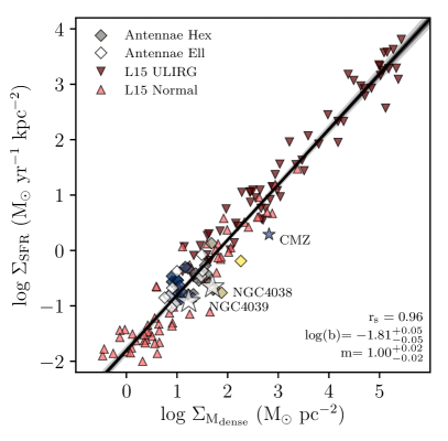
Figure 5.— $\mathrm{\Sigma_{SFR}}$ vs. $\Sigma_{\mathrm{M_{dense}}}$, excluding the data from Gao & Solomon (2004a, b). The symbols and colors are the same as in Figure 4. Liu et al. (2015) calculate source sizes using the radio continuum. Liu et al. (2015) calculate the dense molecular gas mass assuming an HCN conversion factor, $\alpha_{\mathrm{HCN}}=10$ M_⊙ (K km s^-1 pc²). We use the SFRs that Liu et al. (2015) calculate from IR luminosities. The two nuclei of the Antennae have surface densities comparable to those of other regions, and the locus of Antennae points falls in the overlapping regime of normal star-forming galaxies and (U)LIRGs from the Liu et al. (2015) sample. The fit to the Antennae hexagonal datapoints and Liu et al. (2015) datapoints yields a slope of $\mathrm{m}=1.00\pm 0.02$. Upper limits are excluded.

5.2. The nuclei of NGC 4038 and NGC 4039

5.2.1 Low $\mathit{L_{TIR}}/\mathit{L_{dense}}$ and High $\mathit{L_{HCN}}/\mathit{L_{CO}}$

The two nuclei appear to have lower $\mathrm{L_{TIR}}/\mathrm{L_{dense}}$ ratios compared to the ratios of the remaining Antennae regions (see Tables LABEL:tab:ell_lumin, LABEL:tab:ell_props, and LABEL:tab:ell_ratio, and Figure 4). This ratio is taken as a proxy for the star formation efficiency of dense gas, SFE_dense, assuming $\mathrm{L_{TIR}}\propto\mathrm{SFR}$ and $\mathrm{L_{dense}}\propto\mathrm{M_{dense}}$. The estimated SFE_dense for the nuclei are $0.44\times 10^{-8}$ yr^-1 and $0.7\times 10^{-8}$ yr^-1 for NGC 4038 and NGC 4039, respectively, compared to values of $1.1-4.6\times 10^{-8}$ for regions in the overlap and western arm. We compare the $\mathrm{L_{TIR}}/\mathrm{L_{HCN}}$ ratios of the Antennae sources (from elliptical apertures) to those of Gao & Solomon (2004a, b) and Liu et al. (2015) in Figure 4, which shows that the Antennae data, as a whole, span the majority of the range in $\mathrm{L_{TIR}}/\mathrm{L_{HCN}}$ ratios of these two samples of galaxies. This also emphasizes the difference between the two nuclei (white stars) and the overlap and western arm regions (orange diamonds). The nuclei appear on the lower end of the locus of points from Gao & Solomon (2004a, b) and Liu et al. (2015), below the median of the Gao & Solomon (2004a, b) galaxies (850 $\mathrm{L_{\odot}}$ (K km s^-1 pc²)^-1) while the overlap and western arm lie above this value in the typical starburst regime.

The two nuclei also show an enhancement in the $\mathrm{L_{HCN}/L_{CO}}$ ratio relative to the overlap region (Schirm et al., 2016). This line ratio is often used as a proxy for f_dense ($\mathrm{L_{HCN}/L_{CO}\sim M_{dense}/M_{H_{2}}}$), which would indicate that the nuclei have higher dense gas fractions than other regions in the Antennae. Our calculated dense gas fractions are listed in Table LABEL:tab:ell_props, and indeed show that the nuclei have the highest dense gas fractions, with NGC 4038 at $\sim 9.7\%$ and NGC 4039 at $\sim 7.1\%$, compared to $2.2-4.5\%$ for sources in the overlap region. Regions in the western arm exhibit higher dense gas fractions up to $6.9\%$ in WArm-3, although these regions also show higher SFE_dense (e.g. SFE${}_{\mathrm{dense}}=2.19\times 10^{-8}$ yr^-1 in WArm-3), unlike the two nuclei.

This behavior in the nuclei (i.e lower SFE_dense and higher f_dense) is similar to the inner regions of some disk galaxies (e.g. Usero et al. 2015; Bigiel et al. 2016), and could be attributed to an increase in ISM pressure. In some disk galaxies, f_dense has been observed to increase towards the center of the disk/bulge region (e.g. M51 in Bigiel et al. 2016 and the sample of galaxies in Usero et al. 2015), and the star formation efficiency of the dense gas appears to decrease towards the center, showing an inverse correlation with f_dense. This is also coincident with an increase in stellar density and gas fraction observed at the inner radii. If the gas is assumed to be in equilibrium with the hydrostatic pressure in the galaxy then increased ISM pressures arise naturally from this situation (Helfer & Blitz, 1997; Hughes et al., 2013; Bigiel et al., 2016). Then, if the stellar potential were driving up the pressure in the nuclei, we might expect to see overall higher gas surface densities in these regions. Contrary to this, the nuclei appear to have moderate molecular gas surface densities ($\sim$240 and $\sim 510$ M_⊙ pc^-2) compared to the SGMCs in overlap region ($\sim 700-1000$ M_⊙ pc^-2). However, the surface density of the dense gas is higher in the NGC 4038 ($\sim 50$ M_⊙ pc^-2) than in the overlap region ($\sim 30$ M_⊙ pc^-2, while NGC 4039 shows $\Sigma_{\mathrm{Mdense}}=17$ M_⊙ pc^-2. We also note that dynamical equilibrium may not be a valid assumption in a merger system. For example, Renaud et al. (2015) show that cloud-cloud collisions in the Antennae can increase pressure sufficiently through compressive turbulence to be able to produce massive cluster formation. Regardless of the source of increased pressure, it can potentially increase the dense gas content, as well as the mean density of the gas. Loenen et al. (2008) model line ratios in extreme environments such as (U)LIRGs (which are often merger systems) that are consistent with this.

Since the Antennae is a merger system, turbulent pressures are expected to be higher throughout this system (cf. Renaud et al. 2015). Furthermore, the gas in any merger system will be drawn to the higher gravitational potential wells of the nuclei, thus potentially creating an even higher turbulent pressure in these regions. Turbulent pressure may also act to suppress star formation, and is the strongest candidate for explaining the star formation suppression in the Central Molecular Zone (CMZ, Kruijssen et al. 2014). The CMZ is a region known to have high average gas densities ($\mathrm{n(H_{2})>10^{4}}$ cm^-3, Rathborne et al. 2014) despite a relative lack of star formation. Kruijssen et al. (2014) have suggested that the lower SFR is attributed to an overall slower evolution of the gas towards gravitational collapse in the presence of higher turbulence (as the gas density threshold required for star formation is higher). Turbulence is the strongest candidate of the potential star formation suppressors in the CMZ (compared to tidal disruption, gas heating, etc.), and is likely due to gas inflow along the molecular bar or other disk instabilities (Kruijssen et al., 2014). For this scenario to be true, the SFR in the CMZ must be episodic, suggesting that it is currently in a pre-starburst phase. Other evidence suggests that clouds in the CMZ are not strongly self-gravitating (Kauffmann et al., 2017c), but rather are being held together by the stellar potential. This also supports the idea that the SFR in the CMZ may increase in the future as gravitational collapse progresses in this region.

As mentioned previously, starburst episodes are natural in a merger system. If the nuclei are in a pre-(or post-) starburst phase, we may expect to measure higher ISM turbulent pressures from gas inflow (and/or stellar feedback). In the CMZ, pressures are $\mathrm{P/k_{B}}\sim 10^{9}$ K cm^-3 (Rathborne et al., 2014). Previous estimates of the pressure of the warm and cold components of lower-density gas in the Antennae (as measured by CO) show little variation and are $\mathrm{P/k_{B}}\sim 10^{5}$ K cm^-2 (Schirm et al., 2014). However, if mean gas densities are higher in the nuclei, then CO would not adequately trace the bulk properties of gas in these regions. Additionally, HCN/HCO⁺ and HNC/HCN integrated line ratios differ between these sources, indicating that there may be different mechanisms driving the lower SFE_dense and f_dense in each of the two nuclei (Schirm et al., 2016) (NGC 4038 exhibits higher HNC/HCN and HCN/HCO⁺ luminosity ratios than NGC 4039). We investigate variation in the star formation between the two nuclei in §5.2.2.

Rathborne et al. (2014) argue that this lower SFR should be observed in the centers of other galaxies, and more evidence of this behavior is surfacing (e.g. Usero et al. 2015; Bigiel et al. 2016), with more work to come in the future. As discussed above, there are likely a number of sources of turbulence, including stellar feedback. In contrast, enhancements in the $\mathrm{SFE}$ of the total molecular gas content have been observed in the centers of some galaxies (Utomo et al., 2017). Chown et al. (2018) find enhancements in $\mathrm{SFE}$ and central gas concentrations in a number of barred and interacting galaxies, supporting the idea that mass transport can play a significant role in regulating star formation. However, the star formation history of these systems suggest that the enhancements have been sustained over long periods of time. More studies of the dense gas content in these systems will help determine if there is a common relationship between $\mathrm{SFE}$, $\mathrm{SFE_{dense}}$, and $\mathrm{f_{dense}}$ of the centers of barred and interacting galaxies. Overall, the parallels between the CMZ, the centers of disk galaxies, and the nuclei have interesting implications for star formation: processes affecting the SFR and gas PDFs of the CMZ and centers of disk galaxies may also be occurring in disturbed systems such as the Antennae. More work needs to be done to explore the mean density and density profile of the $\mathrm{L_{HCN}}$-emitting gas in these environments.

5.2.2 Star Formation

The two nuclei have the second and third highest L_TIR measurements in the system, below the L_TIR from SGMC345. The SFRs we determine from our L_TIR measurements are 1.14 and 0.63 $\mathrm{M_{\odot}\ yr^{-1}}$, which are higher by a factor $>2$ than the estimates from Brandl et al. (2009). Brandl et al. (2009) use mid-IR fluxes (15 and 30 $\mu$m) to estimate L_TIR, where we use the 24, 70, and 100 $\mu$m fluxes; to compare our estimates with theirs, we apply a scaling factor of 0.86 from Kennicutt & Evans (2012) to their SFR estimates based on the older Kennicutt (1998) SFR calibration. With the scaling factor applied, Brandl et al. (2009) find SFRs to be $0.52$ and $0.27$ M_⊙ yr^-1 for NGC 4038 and NGC 4039, respectively, for L${}_{\mathrm{TIR}}\sim 3.67$ and $1.86\times 10^{9}\ \mathrm{L_{\odot}}$. Using the 70$\ \mu$m flux to estimate L_TIR, Bigiel et al. (2015) find L${}_{\mathrm{TIR}}\sim 8.8$ and $5.5\times 10^{9}\ \mathrm{L_{\odot}}$ for their apertures Nuc. N and Nuc. S, although they do not convert these to SFRs. Our estimates for L_TIR are similar to this, with $\sim 7.67$ and $4.22\times 10^{9}\ \mathrm{L_{\odot}}$. It is likely our apertures are different than those used by Brandl et al. (2009), which may account for some of the differences. Regardless, NGC 4038 appears to have a SFR that is $\sim 2$ times higher than NGC 4039.

NGC 4039 has the characteristics of a post-starburst nucleus with little star formation activity. It hosts an older stellar population ($\sim 65$ Myr from IR spectroscopic results/CO absorption, Mengel et al. 2001) that is dominated by old giants and red supergiants (cf. photospheric absorptions line in the $\sim 2\ \mu$m stellar continuum, Gilbert et al. 2000). Gilbert et al. (2000) found no evidence of Br$\gamma$ emission, which is expected to be present in the atmospheres of young stars. NGC 4039 also has a steep radio spectrum (Neff & Ulvestad, 2000) indicating that the radio emission is originating predominantly from SNe remnants of the $\sim 65$ Myr-starburst. Chandra observations reveal a composite X-ray spectrum that supports this picture: it contains a thermal component (indicating a hot ISM) and steep power-law with $\Gamma\sim 2$ (indicating X-ray binaries, Zezas et al. 2002). Furthermore, Brandl et al. (2009) find evidence that H₂ in NGC 4039 is shock-heated. The lower HNC/HCN ratio we find in NGC 4039 is consistent with these findings and suggests it is driven by the mechanical heating of previous starbust activity and supernovae shocks (Neff & Ulvestad, 2000).

Brandl et al. (2009) find high excitation IR lines in the nucleus of NGC 4039, which is one potential indicator of an accreting stellar black hole binary. They measure a ratio [NIII]/[NII]$\sim 6$ times higher in NGC 4039 than NGC 4038 and strong [S IV], which was not detected in NGC 4038 at all. To determine the source of these high-excitation lines in NGC 4039, Brandl et al. (2009) compare the mid-IR spectral continuum ($\sim 10-30\ \mu$m) to a starburst model template from Groves et al. (2008). They find it matches with a model representative of distributed star formation at solar metallicity, moderate pressures ($\mathrm{P/k_{B}\sim 10^{5}\ K\ cm^{-3}}$), and a PDR fraction indicating star formation is still embedded. Brandl et al. (2009) therefore interpret their line ratios as being consistent with dust emission heated solely by star formation. The [S IV] emission in NGC 4039 may also trace young stars in a $\sim 4-6$ Myr starburst. It is possible an episode of star formation may be in the very early stages in this nucleus. This is again consistent with the picture painted above for the CMZ, as the gas may be in a pre-starburst phase that will eventually go on to form stars at a higher rate. Br$\gamma$ emission is also detected in a circum-nuclear cluster (A1, Gilbert & Graham 2007) which is identified separately from and just north of NGC 4039; however, it falls within our aperture and is likely contributing to our SFR estimates in this region.

NGC 4038 also contains a post-starburst population aged at $\sim 65$ Myr (Mengel et al., 2001). There is evidence of a younger $\sim 6$ Myr population to the north of NGC 4038 (Mengel et al., 2001). NGC 4038 has a very soft X-ray spectrum likely due to thermal emission originating from winds from this region of young star formation (Zezas et al., 2002). Br$\gamma$ emission is detected in the northern nucleus, which provides evidence for young star formation in this region. The X-ray luminosity of NGC 4038 is also lower than that of NGC 4039. Thus, the star formation in NGC 4038 is at a different stage than NGC 4039, and may be at the upswing of a starburst.

5.3. The Western Arm

Whitmore et al. (2010) show that the Antennae presents an interesting number of large- and small-scale patterns related to star formation. One of these regions with such patterns is the western arm. Whitmore et al. (2010) study the population of star clusters in the Antennae using Hubble Space Telescope images from ACS and NICMOS. In the western arm, they designate five knots of clusters (originally discovered by Rubin et al. 1970) that spatially coincide with dense gas emission detected in our study; sources G, L, R, S, and T overlap with our apertures WArm-1 (G), WArm-3 (T, S, and R), and WArm-4 (L). In their study, they note linear spatial age gradients in several clusters, including knots S, T, and L in the western arm. The ages appear to increase towards the inner side of the spiral pattern in the direction of major dust lanes. The dense gas detected along the western arm also appears to be concentrated on the inner portion of the spiral pattern coincident with the dust lanes in this region, excluding WArm-1. (WArm-1 appears more centralized in the northern portion of the spiral pattern.) Whitmore et al. (2010) posit that this gradient may be due either to small-scale processes, such as sequential star formation, or larger-scale processes such as density waves or gas cloud collisions. Either of these processes could also explain the position of the dense gas emission towards the inner portion of the western arm.

The western arm hosts several bright HII regions, as evidenced in the H$\alpha$ image from HST (Fig. 1). The diameters of these hot bubbles are widest along the western arm, indicating slightly more evolved starbursts than the overlap region (Whitmore et al., 2010). The HCN/HCO⁺ ratio varies from $\sim 0.7-1.3$ in this region, with the highest ratio exceeding unity in WArm-3.

WArm-3: The dense gas emission associated with WArm-3 overlaps with the inner edge of the HII region associated with knot S, and likely originates from gas shock-heated by UV winds and SNe. This region also shows bright compact 4- and 6-cm emission with both shallow and steep spectral indices (Neff & Ulvestad, 2000), indicating a combination of thermal emission and synchrotron emission from SN remnants, which could potentially be from the exposed O-star remnants. This is one of the few regions in the Antennae where HCN emission exceeds HCO⁺ (HNC remains very weak/undetected), with HCN also appearing more spatially-extended. The abundance of HCO⁺ can be significantly reduced in environments with a high ionization fraction, while the HCN abundance remains relatively unaffected (Papadopoulos, 2007). This could potentially account for the higher HCN/HCO⁺ ratio here, considering the proximity of this dense gas emission to the HII regions of knots R, S, and T. Or, this region could simply be at an overall higher-density, with mechanical heating continuing to drive down the HNC abundance. Brandl et al. (2009) also study this starbursting region in the western arm (their Peak 4). Age estimates place the stellar population here around $\sim 7$ Myr (Whitmore & Zhang, 2002; Mengel et al., 2005; Brandl et al., 2009). Again, their SFR (0.22 M_⊙ yr^-1) agrees with ours to within $50\%$.

WArm-2: The WArm-2 region, like WArm-3, is coincident with an obscuring dust lane (see Fig. 1). This region does not appear to have compact cm-emission or optical knots associated with it (Neff & Ulvestad, 2000; Whitmore et al., 2010), and it also appears to have the lowest estimated SFR in our sample (0.1 $\mathrm{M_{\odot}}$ yr^-1). There are a few compact HII regions associated with this region (visible in H$\alpha$, Whitmore et al. 2010), indicative of younger, embedded star formation. There is HCO⁺ emission associated with this region, but no detected HCN or HNC. This is consistent with a lower mean density of gas, as both species have higher critical and effective densities than HCO⁺ (Shirley, 2015). It is interesting that HCN is not detected despite there being evidence of star formation in this region. This may indicate that HCN is not an efficient tracer of dense gas at this particular stage of star formation, or perhaps other mechanisms are suppressing the HCN emission that currently remain unclear. It is possible that one or more of these transitions are optically thick and subject to radiative trapping. For example, Jiménez-Donaire et al. (2017) show that radiative trapping can effectively reduce the critical density required to stimulate ¹²C-transitions, thus boosting the intensity of these lines relative to ¹³C-transitions. Something similar could potentially occur between HCO⁺, HCN, and HNC where one or more of these transitions is boosted relative to the other from optical depth variations. However, for optical depth variations to explain HCO⁺ being detected over HCN, HCO⁺ would need a higher optical depth and higher critical density than HCN, which we find unlikely.

Another possible explanation for the detection of HCO⁺ over HCN and HNC is that nitrogen is possibly depleted in WArm-2. A mechanism for this would be low-metallicity gas flowing into the western arm from the outskirts of the galaxy. However, this should affect all regions in the western arm equally, and HCN is detected in WArm-1 and WArm-3. In fact, HCN is brighter than HCO⁺ in WArm-3. Therefore, we find it more likely that the variations we observe are due to excitation effects, such as density variations.

WArm-1: North of WArm-2 is WArm-1, which has visible HCN and HCO⁺ emission. The line ratios for this source are consistent with the average line ratios of the entire system: HCO⁺ is brighter than HCN, and HNC is relatively weak/not detected. There also appear to be optical clusters associated with this region, in particular knot G from Whitmore et al. (2010). Neff & Ulvestad (2000) detect compact radio emission in the vicinity of WArm-1 (their region 13), of which five sources have detections at both 4 and 6 cm and allow for the estimation of their radio spectral indices. Three of these sources have indices $>-0.4$, indicating strong thermal sources, while two have steep non-thermal emission indicated by indices $\sim-0.45$ and $\sim-1.64$. Zezas et al. (2002) detect 18 ultra-luminous X-ray (ULX) sources ($\mathrm{L_{X}}>10^{39}$ erg s^-1) in the Antennae, which they suggest are accreting black hole binaries. One of these sources, their X-ray source 16, is also coincident with the dense gas emission in WArm-1. This is one of three variable ULX sources, which further supports the idea that these are black hole binaries.

WArm-4: The WArm-4 region appears at the southern tail of the spiral pattern. The ratios in this region also follow the average trend of the system. Again, optical clusters (knot L, Whitmore et al. 2010) and compact radio emission (region 8, Neff & Ulvestad 2000) are associated with this region. The region of compact radio emission associated with knot L has a spectral index that indicates thermal emission is the dominant source ($\sim 0.18$, Neff & Ulvestad 2000). There appear to be no medium/hard X-ray sources associated with this region, although there is diffuse soft X-ray emission throughout the Antennae (Zezas et al., 2002).

5.4. The Overlap Region

We find our SFR estimates are systematically lower for the SGMCs in the overlap region than the estimates from Brandl et al. (2009), perhaps related to the different TIR calibrators used. For clouds in the overlap region, Brandl et al. (2009) estimate 0.61 M_⊙ yr^-1 for SGMC 1 (their Peak 3, corrected) and 3.14 M_⊙ yr^-1 for SGMC345 (the addition of their measurements for their Peaks 1 and 2, corrected). Our estimate for SGMC 2 (their Peak 5), 0.63 M_⊙ yr^-1, agrees well with their value of 0.55 M_⊙ yr^-1 (corrected). Brandl et al. (2009) suggest that L_TIR estimates may be high for regions with stellar populations $<10$ Myr; this in particular would affect measurements in the overlap region, which contains stellar populations as young as $\sim 2-5$ Myr (Brandl et al., 2009; Whitmore & Zhang, 2002; Mengel et al., 2005; Gilbert & Graham, 2007; Snijders et al., 2007). Additionally, mid-IR fluxes are more sensitive to younger stellar populations (Kennicutt & Evans, 2012), and these wavelengths may be better tracers of star formation in the overlap region; this could explain the discrepancy between our measurements (from 24, 70, and 100 $\mu$m IR observations) and those from Brandl et al. (2009), implying our estimates may be low.

There are numerous studies on star formation in the overlap region, with recent high-resolution ALMA studies now revealing the formation of super-star clusters (SSCs) (Whitmore et al., 2010; Johnson et al., 2015; Herrera & Boulanger, 2017). At higher resolution, it is easier to distinguish the individual SGMCs, their associated clusters, and the conditions accompanying them. Theoretical studies of SSCs suggest that they require high pressures ($\mathrm{P/k_{B}}\sim 10^{7}-10^{8}$ K cm^-3) are required for their formation (Herrera & Boulanger, 2017). As mentioned above, Schirm et al. (2014) found moderate pressures across the entire system, $\mathrm{P/k_{B}}\sim 10^{5}$ K cm^-3 using an excitation analysis of multiple-$J$ transitions of CO. However, these observations were using lower-resolution data ($\sim 43^{\prime\prime}$) which likely will not capture the conditions necessary to form SSCs, since these form on much smaller scales. The existence of SSCs in the overlap region strongly suggests that gas pressures are higher than these previous estimates.

Our apertures in the overlap region coincide with bright star-forming knots B (our aperture SGMC345), C, and D (Rubin et al. 1970; Whitmore et al. 2010, our SGMC1), and a more extended star-forming region 2 (Whitmore & Schweizer 1995, our SGMC2, C6, C7, and C8*). Our C9* region is adjacent (west) to star-forming knot B and does not coincide with bright optical star-forming regions. The strongest thermal radio source in Neff & Ulvestad (2000) lies in the overlap region and falls within our aperture SGMC345. More specifically, this thermal source is overlapping with SGMCs 4 and 5, with SGMC 3 off further to the west. Neff & Ulvestad (2000) estimate that $\sim 5000$ O5 stars would be required to ionize this gas, resulting in an absolute magnitude of $-15$, or 500,000 B0 resulting in a magnitude of $-18$, bright enough to be detected with HST if the starlight is not obscured by foreground dust or gas. However, Whitmore & Schweizer (1995) do not detect bright cluster emission near this radio source. Therefore, Neff & Ulvestad (2000) suggest that star formation must be embedded in this particular complex, hidden by optical extinction that is at least 4 orders of magnitude. We measure the highest SFR in SGMC345, 1.46 $\mathrm{M_{\odot}}$ yr^-1, which is consistent with this being the most vigorously star-forming complex in the Antennae.

5.5. Conversion Factors

We use the $\mathrm{L_{HCN}/L_{CO}}$ ratio as an estimator of dense gas fraction across the Antennae assuming constant conversion factors, $\alpha_{\mathrm{HCN}}$ and $\alpha_{\mathrm{CO}}$. However, if $\alpha_{\mathrm{HCN}}$ and $\alpha_{\mathrm{CO}}$ vary across the Antennae, the trends we see between $\mathrm{L_{TIR}}$, $\mathrm{L_{HCN}}$, and $\mathrm{L_{CO}}$ may not be a consequence of different dense gas fractions. In particular, the CO conversion factor can vary with several gas properties, including metallicity, CO abundance, temperature, and gas density variations (cf. Bolatto et al. 2013). Using computational models, Narayanan et al. (2011) study the effects of varying physical properties on $\alpha_{\mathrm{CO}}$ in disks and merging systems, and they find $\alpha_{\mathrm{CO}}$ is typically lower in regions of active star formation in merger-driven starbursts. This is primarily due to higher gas temperatures and larger gas velocity dispersions in these systems (from increased thermal dust-gas coupling). They also show that $\alpha_{\mathrm{CO}}$ can either stay low or rebound after the starburst phase ends, depending on H₂ or CO abundances and the time required to revirialize gas. If we extrapolate these results to the $\sim$kpc scales studied in the Antennae, one would expect the overlap region to have a smaller $\alpha_{\mathrm{CO}}$ than the two nuclei, as this is the most vigorously star forming region in the merger.

However, Zhu et al. (2003) find evidence that the CO conversion factor may be 2-3 times lower in NGC 4038 than in the overlap region using Large Velocity Gradient (LVG) modelling of multiple ¹²CO and ¹³CO transitions. They find $\mathrm{X_{CO}}\sim(5.1-6.4)\times 10^{19}(10^{-4}/{x_{\mathrm{CO}}})$ cm^-2 (K km s^-1)^-1 in the overlap region and $\mathrm{X_{CO}}\sim 2.3\times 10^{19}(10^{-4}/{x_{\mathrm{CO}}})$ cm^-2 (K km s${}^{-1})^{-1}$ for NGC 4038, where $\mathrm{X_{CO}}$ is the two-dimensional conversion factor, $\Delta\mathrm{V}$ is the line width, and $x_{\mathrm{CO}}$ is the CO abundance relative to H₂ (the CO abundance is typically $x_{\mathrm{CO}}\sim 10^{-5}-10^{-4}$ in starbursts, Booth & Aalto 1998; Mao et al. 2000). Zhu et al. (2003) argue that the lower conversion factor in NGC 4038 is due to high velocity dispersion, large filling fraction, and low optical depth of the CO-emitting gas. Sandstrom et al. (2013) show that the CO conversion factor is lower by a factor of $\sim 2$ (on average) in the central 1 kpc of a sample of 26 star-forming disk galaxies, and they also find that it can be up to 10 times lower than the standard Milky Way value ($\alpha_{\mathrm{CO}}=4.4$ M_⊙ pc^-2 (K km s^-1)^-1)). Sandstrom et al. (2013) suggest several explanations for this discrepancy in $\alpha_{\mathrm{CO}}$ in the central regions of these galaxies, including differences in ISM pressure, higher molecular gas temperatures, and/or more diffuse ISM molecular gas; optical depth variations can also alter the conversion factor of the gas and can act in accordance with any of the previous effects.

It is possible that the effects on $\alpha_{\mathrm{CO}}$ in galaxy centers observed in the Sandstrom et al. (2013) sample could still apply to the two nuclei in the Antennae. If $\alpha_{\mathrm{CO}}$ is indeed lower in NGC 4038, this would decrease the total molecular mass estimates in that nucleus and would increase the dense gas fraction in NGC 4038, thus exacerbating the difference between this nucleus and the overlap region. Metallicities have been found for young and intermediate stellar clusters across the Antennae ranging from slightly sub-solar to super-solar (Z$=0.9-1.3$ Z_⊙, Bastian et al. 2009), but there are no obvious differences between clusters near the two nuclei vs those in the overlap region. High-resolution observations resolving gas at $\sim$kpc scales of multiple CO transitions have yet to be done in the Antennae and therefore gas properties such as density, temperature, and abundance are not constrained at these scales.

The conversion between HCN luminosity and dense gas mass is not as well studied as the CO conversion factor, but the HCN conversion factor is derived using the same principles assumed for $\alpha_{\mathrm{CO}}$. Thus, $\alpha_{\mathrm{HCN}}$ may also change with metallicity, pressure, temperature, density, etc. Observations of HCN and HCO⁺ lines in (U)LIRGs suggest that HCN can experience a large range of excitation conditions (e.g. Papadopoulos 2007; Papadopoulos et al. 2014), with some of these extreme galaxies showing sub-thermal HCN emission (i.e. Mrk 231, Papadopoulos 2007). Galactic observations of HCN in Orion A also show that HCN can be excited at more moderate densities, $\mathrm{n}\sim 10^{3}$ cm^-3 (Kauffmann et al., 2017a), missing dense gas entirely in some star-forming environments. Shimajiri et al. (2017) directly compare HCN $\mathrm{J}=1-0$ emission and dust column density maps in three Galactic star-forming clumps and find evidence that $\alpha_{\mathrm{HCN}}$ may decrease with increasing local FUV radiation field, $\mathrm{G}_{0}$. In an attempt to calibrate $\alpha_{\mathrm{HCN}}$ numerically, Onus et al. (2018) study the dependence of $\alpha_{\mathrm{HCN}}$ on different physical conditions using simulations of star-forming gas at $\sim 2$ pc scales. They find that variations in HCN abundance ($3.3\times 10^{-9}$ vs $3\times 10^{-8}$) change $\alpha_{\mathrm{HCN}}$ by a factor of $\sim 2$, and that moderate differences in temperature (10 vs 20 K) can also alter $\alpha_{\mathrm{HCN}}$, but less significantly. So far these observations and simulations have been limited to small spatial scales (on the order of $\sim$10 pc). At these smaller scales, there is some expected stochasticity of physical conditions within molecular clouds that may affect $\alpha_{\mathrm{HCN}}$. For applications to extragalactic observations, this work needs to be expanded to larger scales (kiloparsecs) to better estimate $\alpha_{\mathrm{HCN}}$.

5.6. Dense Gas Fractions

Traditionally, the dense gas fraction is estimated as the direct ratio of total molecular mass (traced by CO) to dense gas mass (traced by HCN). This works under the assumption that CO is tracing the mean density of gas, while HCN is tracing only the high-density gas that is more directly associated with star formation. However, recent work on the CMZ suggests that this may be an oversimplification; Kruijssen et al. (2014) show that the overall gas density PDF can be pushed to significantly higher densities via turbulence, while the gas densities more directly associated with star formation are even higher (Rathborne et al., 2014). In this regime, HCN is a better tracer of the mean density of gas. Therefore, our interpretation of the $\mathrm{L_{TIR}}/\mathrm{L_{dense}}$ and $\mathrm{L_{HCN}}/\mathrm{L_{CO}}$ ratios may vary depending on the regime of star formation we are in.

Current turbulent models of star formation predict lognormal gas density PDFs that evolve to have power-law tails once gravitational collapse begins in the process of star formation (e.g. Federrath & Klessen 2012). Gravitational collapse will begin once the gas reaches a threshold density that is high enough to overcome pressure support in the cloud. If the source of pressure is turbulence, it can act to (1) widen the gas density PDF, and/or (2) push the overall mean density of the gas to higher values (Federrath & Klessen, 2012). In this case, we may expect to see an enhancement of luminosities of dense gas tracers, such as HCN, relative to lower-density gas tracers such CO (cf. Leroy et al. 2017).

We suggested in §5.2.1 that similar effects of the gas and star formation in the CMZ may be affecting the two nuclei in the Antennae. If the gas density PDF is indeed shifted to higher densities in the nuclei, this may result in a smaller HCN conversion in these regions, which would decrease the dense gas fraction in these regions. For example, turbulence in the CMZ has the effect of driving up the mean density of gas to $\mathrm{n(H_{2})\sim}10^{4}$ cm^-3, which is 100 times larger than the mean density of GMCs elsewhere in the Milky Way (Rathborne et al., 2014). Similarly, the threshold of gas required for star formation (also referred to as a critical density in some literature) in the CMZ is also higher, $\mathrm{n(H_{2})_{thresh}\sim}10^{6}$ cm^-3 (Rathborne et al., 2014). Therefore, an accurate measure of dense gas fraction in this region is a comparison of the mass at densities $>10^{6}$ cm^-3, M($>10^{6}$ cm^-3), to that of the total molecular gas content. In the CMZ, HCN can be well-excited already at $\mathrm{n(H_{2})\sim}10^{4}$ cm^-3, the mean density of the gas. This makes HCN a better tracer of the mean density of gas in the CMZ, rather than CO. Similar effects likely affect the luminosity measurements in the nuclei of the Antennae.

6. Conclusion

We present a study of the dense gas content and star formation in NGC 4038/9, with detections of HCN, HCO⁺, and HNC J=1-0 emission in four distinct regions of the Antennae: the two nuclei (NGC 4038, NGC 4039), the overlap region, and the western arm. We consider the two nuclei separately as they exhibit differences in dense gas line ratios and star formation activity.

1. The two nuclei show a suppression in the $\mathrm{L_{TIR}/L_{HCN}}$ ratio, despite showing an enhanced $\mathrm{L_{HCN}/L_{CO}}$ ratio, when compared with the overlap and western arm regions. Assuming constant conversion factors, $\alpha_{\mathrm{HCN}}$ and $\alpha_{\mathrm{CO}}$, this suggests the two nuclei have a higher dense gas fraction and lower star formation efficiency of dense gas compared to the rest of the Antennae. One potential explanation for this is an increase in overall turbulence in these regions that acts to suppress star formation while also increasing the overall gas density, similar to what appears to be happening in the CMZ in the Milky Way (Kruijssen et al., 2014). This behavior is expected in the pre-starburst phase of merger systems (Narayanan et al., 2011).

2. The Antennae data extend the $\mathrm{L_{TIR}\ vs.\ L_{HCN}}$ relationship observed by Gao & Solomon (2004a, b) to lower luminosity, consistent with the results from Bigiel et al. (2015). The Antennae datapoints fit within the scatter of the (Gao & Solomon, 2004a, b) and Liu et al. (2015) datapoints. A fit of the Antennae data with that of Liu et al. results in a power-law index of m$\sim$1.

3. A fit to the Antennae $\mathrm{L_{TIR}}$ and $\mathrm{L_{HCN}}$ data shows a sub-linear relationship with a power law index m$\sim$0.5 (hexagonal apertures). Fits with $\mathrm{L_{HCO^{+}}}$ and $\mathrm{L_{HNC}}$ similarly show sub-linear power law indices of m$\sim$0.5 and m$\sim$0.6, respectively. Assuming L${}_{\mathrm{TIR}}\sim$SFR and $\mathrm{L_{HCN}}\sim$M_dense, this indicates of variations in the star formation efficiency of dense gas across this system, such that SFE_dense does not increase directly with M_dense.

4. Except for NGC 4038 and WArm-3, the HCN/HCO⁺ ratio is less than unity for regions in the Antennae, and HNC is significantly weaker than HCN and HCO⁺. These average line ratios of HCN, HCO⁺, and HNC are consistent with a lower-density ($\mathrm{n<10^{5}}$ cm^-3) PDR dominated by mechanical heating from stellar UV- and SNe shock-driven chemistry (Loenen et al., 2008).

5. Schirm et al. (2016) revealed bright, dense gas emission in the overlap region and two nuclei. At the tapered resolution of this study, bright HCN and HCO⁺ J$=1-0$ emission is also detected along the inner portion of the western arm of the Antennae, which also coincides with a dust lane. Stellar clusters show age gradients, increasing in age towards the inner portion of the arm. Since this coincides with bright dense gas emission and dust, this supports the idea that the clusters formed via sequential star formation, or larger-scale processes such as density waves or gas cloud collisions (Whitmore et al., 2014).

Acknowledgements

We thank the referee for their comments which have helped to improve the paper. This paper makes use of the following ALMA data: ADS/JAO.ALMA$\#$2012.1.1.00185.S. ALMA is a partnership of ESO (representing its member states), NSF (USA) and NINS (Japan), together with NRC (Canada), MOST and ASIAA (Taiwan), and KASI (Republic of Korea), in cooperation with the Republic of Chile. The Joint ALMA Observatory is operated by ESO, AUI/NRAO and NAOJ. The National Radio Astronomy Observatory is a facility of the National Science Foundation operated under cooperative agreement by Associated Universities, Inc. This work is based in part on observations made with the Spitzer Space Telescope, which is operated by the Jet Propulsion Laboratory, California Institute of Technology under a contract with NASA. Part of this work is based on observations made with Herschel. Herschel is an ESA space observatory with science instruments provided by European-led Principal Investigator consortia and with important participation from NASA. AB wishes to acknowledge partial support from an Ontario Trillium Scholarship (OTS). CDW acknowledges financial support from the Canada Council for the Arts through a Killam Research Fellowship. The research of CDW is supported by grants from the Natural Sciences and Engineering Research Council of Canada and the Canada Research Chairs program. This research made use of Astropy, a community-developed core Python package for Astronomy The Astropy Collaboration et al. (2018). A significant amount of this research also made use of Matplotlib (Hunter, 2007), Photutils (Bradley et al., 2016), Numpy (Van Der Walt et al., 2011), and Pandas (Mckinney, 2010) Python packages. This research has made use of the NASA/IPAC Extragalactic Database (NED) which is operated by the Jet Propulsion Laboratory, California Institute of Technology, under contract with the National Aeronautics and Space Administration. This research has made use of NASA’s Astrophysics Data System Bibliographic Services.

Appendix A Uncertainties

A.I. Molecular Luminosities

There are three primary sources of uncertainty on the molecular luminosities that we consider: 1. the calibration uncertainty of the ALMA data ($\sim 5\%$ for Band 3, ALMA Technical Handbook for Cycle 1), 2. the rms uncertainty of the moment zero maps, and 3. the uncertainty on the luminosity distance from Schweizer et al. (2008) that we use. The rms uncertainty per aperture is discussed in §3 and given by equation 3. There is a $5\%$ flux calibration uncertainty on each pixel that adds with the distance and aperture rms uncertainties in quadrature:

$$\sigma_{\mathrm{L^{\prime}}} =\mathrm{L^{\prime}}\sqrt{\left(\mathrm{\frac{\sigma_{M_{0},ap}}{M_{0,{ap}}}}\right)^{2}+\mathrm{(0.05)^{2}}+2\left(\mathrm{\frac{\sigma_{D_{L}}}{D_{L}}}\right)^{2}}$$

A.II. Infrared Measurements and Luminosities

Uncertainty maps of the Herschel and Spitzer data are included in each of the downloaded fits files (created by the relevant reduction software) and describe the instrumental uncertainty, such that each pixel has an associated value and uncertainty: $\mathrm{S}_{\nu}\mathrm{(x,y})\pm\sigma_{\mathrm{inst},\nu}\mathrm{(x,y)}$. Each of the instruments have a flux calibration uncertainty that also needs to be folded into the total uncertainty estimate of each pixel, $\sigma_{\mathrm{cal}}$, which are 5%, 5%, and 4% for PACS (Poglitsch et al., 2010), SPIRE (Griffin et al., 2010), and MIPS (Bendo et al., 2012a), respectively. For each of the IR maps, we estimate the background level using three, separate apertures selected within the flat region of the background in each map. The average of this background level is subtracted from our measurements, and the corresponding background-subtraction uncertainty, $\sigma_{\mathrm{back,\nu}}$, is also folded into our final measurement uncertainties. The absolute uncertainty on the flux in a single pixel, $\mathrm{S}_{\nu}$, can be written:

$$\sigma_{\mathrm{S}_{\nu}}\mathrm{(x,y)} =\sqrt{\sigma_{\mathrm{inst},\nu}\mathrm{(x,y)}^{2}+(\sigma_{\mathrm{cal}}\times\mathrm{S}_{\nu}\mathrm{(x,y)})^{2}+\sigma_{\mathrm{back,\nu}}^{2}}$$

We convert IR fluxes to single-band luminosities using Eq. 2, so the absolute uncertainty on these luminosities at pixel (x,y) can be written (incorporating the distance uncertainty) as:

$$\mathrm{\sigma_{\nu L_{\nu}}(\mathrm{x,y})=\nu L_{\nu}(\mathrm{x,y})\sqrt{2\left(\frac{\sigma_{d_{L}}}{d_{L}}\right)^{2}+\left(\frac{\sigma_{S_{\nu}}(\mathrm{x,y})}{S_{\nu}(\mathrm{x,y})}\right)^{2}}}$$

The monochromatic $\mathrm{L_{TIR}}$ calibrations from Galametz et al. (2013) are given in the form $\mathrm{log(L_{TIR})={a_{i}{log}(\nu_{i}L_{\nu,i})+b_{i}}}$, where $\mathrm{a_{i}\pm\sigma_{a_{i}}}$ and $\mathrm{b_{i}\pm\sigma_{b_{i}}}$ are fit parameters and their uncertainties for IR band i. To derive the uncertainty on $\mathrm{log(L_{TIR})}$, we use standard error propagation:

$$\sigma_{\mathrm{log(L_{TIR})}} =\mathrm{\sqrt{\left(log(\nu L_{\nu,i})\sigma_{a,i}\right)^{2}+\sigma_{b,i}^{2}+\left(\frac{a_{i}\sigma_{L_{\nu,i}}}{L_{\nu,i}ln(10)}\right)^{2}}}$$

where the absolute uncertainty on the total infrared luminosity is then:

$$\sigma_{L_{\mathrm{TIR}}}=L_{\mathrm{TIR}}\mathrm{ln}10\sigma_{\mathrm{log}L_{\mathrm{TIR}}}$$

The Galametz et al. (2013) calibrations combining more than one IR band are in the form $\mathrm{L}_{\mathrm{TIR}}=\sum_{i}{c_{i}\nu L_{\nu}(i)}$ where $c_{i}\pm\sigma_{c_{i}}$ are the fit parameters and their uncertainties for band $i$. The uncertainties on $\mathrm{L}_{\mathrm{TIR}}$ are then:

$$\sigma_{\mathrm{L}_{\mathrm{TIR}}} =\sqrt{\sum_{i}\left(c_{i}\sigma_{\nu L_{\nu}(i)}\right)^{2}+\left(\nu L_{\nu}(i)\sigma_{c_{i}}\right)^{2}}$$

Galametz et al. (2013) suggest an uncertainty of $\sim 50\%$ on the monochromatic $\mathrm{L}_{\mathrm{TIR}}$ estimates, and an uncertainty of $\sim 30\%$ on those combining multiple bands. Therefore, we cite the uncertainties that are largest (i.e. the percentage uncertainty from Galametz et al. (2013) vs. our absolute uncertainty derivations).

Appendix B $\mathrm{L_{TIR}}$ Calibrations

We expect the $\mathrm{L_{TIR}}(24+70+100+160+250)$ calibration from Galametz et al. (2013) puts the tightest constraints on the total infrared luminosity estimate since it most precisely reproduces the modelled $\mathrm{L_{TIR}}$ estimates in Galametz et al. (2013) in comparison to the calibrations using fewer bands. Therefore, we compare other calibrations with just the higher-resolution IR data (i.e. 24, 70, and 100 $\mu$m maps) to this calibration to assess their spatial variation across the Antennae. We show ratios of these $\mathrm{L_{TIR}}$ calibrations to the $\mathrm{L_{TIR}}(24+70+100+160+250)$ at the 250 $\mu$m resolution in Figure 6. The $\mathrm{L_{TIR}}(24+100)$ and $\mathrm{L_{TIR}}(24+70+100)$ show the least spatial variation when compared to the $\mathrm{L_{TIR}}(24+70+100+160+250)$ calibration and agree well (ratio$\approx$1) with this estimate. The remaining calibrations tend to predict higher or lower values in the overlap, particularly near SGMC345.

The $\mathrm{L_{TIR}}(24+100)$ weights the 24 $\mu$m and 100 $\mu$m fluxes with coefficients of $2.453\pm 0.085$ and $1.407\pm 0.013$, while the $\mathrm{L_{TIR}}(24+70+100)$ calibration coefficients are $2.192\pm 0.114$, $0.187\pm 0.035$, and $1.314\pm 0.016$ for the 24, 70, and 100 $\mu$m fluxes, respectively. The 24 $\mu$m and 100 $\mu$m fluxes appear to be similarly-weighted across these two calibrations, with the 70 $\mu$m flux being weighted relatively low for $\mathrm{L_{TIR}}(24+70+100)$. In comparison to the other calibrations which use the 70 $\mu$m flux, this is the lowest 70 $\mu$m coefficient. Because of the low/non-dependence of these calibrations on the 70 $\mu$m flux, these appear to reduce the (potential) effect of dust heating in the strong-starbursting environment of SGMC345. See §2.2 for the remainder of our discussion on the variation of different Galametz et al. (2013) calibrations.

Galametz et al. (2013) find the Herschel 100$\mu$m band to be the best monochromatic estimate for L_TIR for their sample of galaxies (it is within $30\%$ of their SED-modelled L_TIR estimates). This calibration also shows little variation when compared with their modelled L_TIR (see Figure 7 in Galametz et al. 2013) as a function of the 70/100 color. The outliers of the 100 $\mu$m relationship were mainly strongly starbursting galaxies, NGC 1377 and NGC 5408, with SED peaks at lower IR wavelengths, $\sim$ 60 and 70 $\mu$m, respectively. Galametz et al. (2013) find the 70 $\mu$m band tends to overestimate lower IR luminosity objects (L${}_{\mathrm{TIR}}<3\times 10^{8}\ \mathrm{L}_{\odot}$) and suggest using the 70 $\mu$m band as an estimator for starbursting objects. Similarly, Galametz et al. (2013) find the 160 $\mu$m calibration tends to underestimate L_TIR for hot objects, like starbursts or low-metallicity objects, and overestimate L_TIR for cooler objects. The 70 and 160 $\mu$m calibrations provide reasonable estimates of L_TIR to within $<50\%$, but Galametz et al. (2013) suggest that the 70 and 160 $\mu$m calibrations are used with caution for hot or cold SEDs. Klaas et al. (2010) plot IR SEDs of several clumps that are identified in $24-160\ \mu$m maps of the Antennae and find that the SED shape agrees well for most regions across this wavelength range, with peaks at $\sim 100\ \mu$m. However, one clump in their study (which corresponds to the region in the overlap with SGMC345) shows a higher $24/70$ ratio ($\sim 0.15$ vs. $\sim 0.04-0.08$), with a hotter SED (peak at $\sim 70\ \mu$m). With this in mind, we compare L_TIR from several multi-band L_TIR calibrations from Galametz et al. (2013) in Figure 6 and Table B.

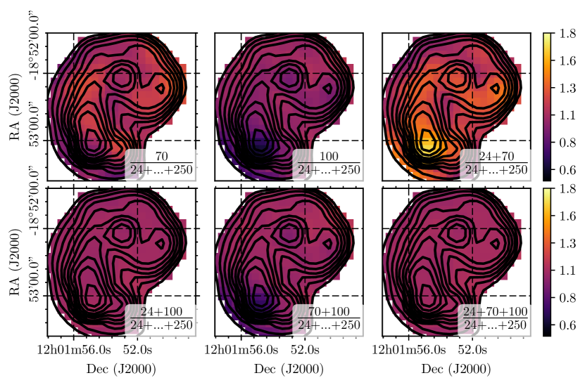
Figure 6.— Ratio maps of Galametz et al. (2013) calibrations at the 250 $\mu$m resolution ($18.1^{\prime\prime}$) with 250 $\mu$m contours overlaid. The $\mathrm{L_{TIR}}(24+70+100+160+250)$ calibration puts the tightest constraints on the total infrared luminosity estimate, therefore we compare combinations of calibrations with just the higher-resolution IR data (i.e. 24, 70, and 100 $\mu$m maps) to this calibration. Top, left to right: $\mathrm{L_{TIR}}(70)/\mathrm{L_{TIR}}(24+70+100+160+250)$, $\mathrm{L_{TIR}}(100)/\mathrm{L_{TIR}}(24+70+100+160+250)$, $\mathrm{L_{TIR}}(24+70)/\mathrm{L_{TIR}}(24+70+100+160+250)$. Bottom, left to right: $\mathrm{L_{TIR}}(70+100)/\mathrm{L_{TIR}}(24+70+100+160+250)$, $\mathrm{L_{TIR}}(24+100)/\mathrm{L_{TIR}}(24+70+100+160+250)$, $\mathrm{L_{TIR}}(24+70+100)/\mathrm{L_{TIR}}(24+70+100+160+250)$.

Table 5Total Infrared Luminosities from Different Calibrations

Appendix C Luminosity Ratios

We include line luminosity ratios in Table LABEL:tab:ell_ratio for the elliptical apertures. The table is divided into three sections: 1. The HCN and HCO⁺ luminosity relative to CO. 2. The total infrared luminosity relative to CO, HCN, and HCO⁺, and 3. Ratios of our three dense gas tracers, HCN, HCO⁺, and HNC.

• Note. – Luminosities measured from the elliptical apertures listed in Table 3. All values are measured at the 100 $\mu$m resolution (6.8^′′). The absolute uncertainties are shown next to each ratio, except in the case of limits. We do not show ratios when both luminosity measurements are limits.

References

- Aniano et al. (2011) Aniano, G., Draine, B. T., Gordon, K. D., & Sandstrom, K. 2011, PASP, 123, 1218
- Bastian et al. (2009) Bastian, N., Trancho, G., Konstantopoulos, I. S., & Miller, B. W. 2009, ApJ, 701, 607
- Bendo et al. (2012a) Bendo, G. J., Galliano, F., & Madden, S. C. 2012a, MNRAS, 423, 197
- Bendo et al. (2012b) Bendo, G. J., Boselli, A., Dariush, A., et al. 2012b, MNRAS, 419, 1833
- Bigiel et al. (2015) Bigiel, F., Leroy, A. K., Blitz, L., et al. 2015, ApJ, 815, 103
- Bigiel et al. (2016) Bigiel, F., Leroy, A. K., Jiménez-Donaire, M. J., et al. 2016, ApJ, 822, L26
- Bolatto et al. (2013) Bolatto, A. D., Wolfire, M., & Leroy, A. K. 2013, ARA&A, 51, 207
- Booth & Aalto (1998) Booth, R. S., & Aalto, S. 1998, The Molecular Astrophysics of Stars and Galaxies, edited by Thomas W. Hartquist and David A. Williams. Clarendon Press, Oxford, 1998., p.437, 4, 437
- Bradley et al. (2016) Bradley, L., Sipocz, B., Robitaille, T., et al. 2016, astropy/photutils: v0.3, doi:10.5281/zenodo.164986
- Brandl et al. (2009) Brandl, B. R., Snijders, L., den Brok, M., et al. 2009, ApJ, 699, 1982
- Chen et al. (2015) Chen, H., Gao, Y., Braine, J., & Gu, Q. 2015, ApJ, 810, 140
- Chown et al. (2018) Chown, R., Li, C., Li, N., et al. 2018, ArXiv e-prints, arXiv:1810.08624
- Daddi et al. (2010) Daddi, E., Elbaz, D., Walter, F., et al. 2010, ApJ, 714, L118
- Federrath & Klessen (2012) Federrath, C., & Klessen, R. S. 2012, ApJ, 761, 156
- Galametz et al. (2013) Galametz, M., Kennicutt, R. C., Calzetti, D., et al. 2013, MNRAS, 431, 1956
- Gallagher et al. (2018) Gallagher, M. J., Leroy, A. K., Bigiel, F., et al. 2018, ApJ, 858, 90
- Gao & Solomon (2004a) Gao, Y., & Solomon, P. M. 2004a, ApJS, 152, 63
- Gao & Solomon (2004b) —. 2004b, ApJ, 606, 271
- Gilbert & Graham (2007) Gilbert, A. M., & Graham, J. R. 2007, ApJ, 668, 168
- Gilbert et al. (2000) Gilbert, A. M., Graham, J. R., McLean, I. S., et al. 2000, ApJ, 533, L57
- Graciá-Carpio et al. (2008) Graciá-Carpio, J., García-Burillo, S., Planesas, P., Fuente, A., & Usero, A. 2008, A&A, 479, 703
- Griffin et al. (2010) Griffin, M. J., Abergel, A., Abreu, A., et al. 2010, A&A, 518, L3
- Groves et al. (2008) Groves, B., Dopita, M. A., Sutherland, R. S., et al. 2008, ApJS, 176, 438
- Hao et al. (2011) Hao, C.-N., Kennicutt, R. C., Johnson, B. D., et al. 2011, ApJ, 741, 124
- Helfer & Blitz (1997) Helfer, T. T., & Blitz, L. 1997, ApJ, 478, 162
- Herrera & Boulanger (2017) Herrera, C. N., & Boulanger, F. 2017, A&A, 600, A139
- Hughes et al. (2013) Hughes, A., Meidt, S. E., Colombo, D., et al. 2013, ApJ, 779, 46
- Hunter (2007) Hunter, J. D. 2007, Computing In Science & Engineering, 9, 90
- Jiménez-Donaire et al. (2017) Jiménez-Donaire, M. J., Bigiel, F., Leroy, A. K., et al. 2017, MNRAS, 466, 49
- Johnson et al. (2015) Johnson, K. E., Leroy, A. K., Indebetouw, R., et al. 2015, ApJ, 806, 35
- Jones et al. (2012) Jones, P. A., Burton, M. G., Cunningham, M. R., et al. 2012, MNRAS, 419, 2961
- Karl et al. (2010) Karl, S. J., Naab, T., Johansson, P. H., et al. 2010, ApJ, 715, L88
- Kauffmann et al. (2017a) Kauffmann, J., Goldsmith, P. F., Melnick, G., et al. 2017a, A&A, 605, L5
- Kauffmann et al. (2017b) Kauffmann, J., Pillai, T., Zhang, Q., et al. 2017b, A&A, 603, A89
- Kauffmann et al. (2017c) —. 2017c, A&A, 603, A90
- Kelly (2007) Kelly, B. C. 2007, ApJ, 665, 1489
- Kennicutt & Evans (2012) Kennicutt, R. C., & Evans, N. J. 2012, ARA&A, 50, 531
- Kennicutt (1998) Kennicutt, Jr., R. C. 1998, ARA&A, 36, 189
- Kepley et al. (2014) Kepley, A. A., Leroy, A. K., Frayer, D., et al. 2014, ApJL, 780, L13
- Klaas et al. (2010) Klaas, U., Nielbock, M., Haas, M., Krause, O., & Schreiber, J. 2010, A&A, 518, L44
- Kruijssen et al. (2014) Kruijssen, J. M. D., Longmore, S. N., Elmegreen, B. G., et al. 2014, MNRAS, 440, 3370
- Krumholz & McKee (2005) Krumholz, M. R., & McKee, C. F. 2005, ApJ, 630, 250
- Lada et al. (2012) Lada, C. J., Forbrich, J., Lombardi, M., & Alves, J. F. 2012, ApJ, 745, 190
- Lada et al. (1991a) Lada, E. A., Bally, J., & Stark, A. A. 1991a, ApJ, 368, 432
- Lada et al. (1991b) Lada, E. A., Depoy, D. L., Evans, II, N. J., & Gatley, I. 1991b, ApJ, 371, 171
- Leroy et al. (2016) Leroy, A. K., Hughes, A., Schruba, A., et al. 2016, ApJ, 831, 16
- Leroy et al. (2017) Leroy, A. K., Usero, A., Schruba, A., et al. 2017, ApJ, 835, 217
- Liu et al. (2015) Liu, L., Gao, Y., & Greve, T. R. 2015, ApJ, 805, 31
- Loenen et al. (2008) Loenen, A. F., Spaans, M., Baan, W. A., & Meijerink, R. 2008, A&A, 488, L5
- Mao et al. (2000) Mao, R. Q., Henkel, C., Schulz, A., et al. 2000, A&A, 358, 433
- Mckinney (2010) Mckinney, W. 2010
- McMullin et al. (2007) McMullin, J. P., Waters, B., Schiebel, D., Young, W., & Golap, K. 2007, in Astronomical Society of the Pacific Conference Series, Vol. 376, Astronomical Data Analysis Software and Systems XVI, ed. R. A. Shaw, F. Hill, & D. J. Bell, 127
- Meijerink & Spaans (2005) Meijerink, R., & Spaans, M. 2005, A&A, 436, 397
- Meijerink et al. (2007) Meijerink, R., Spaans, M., & Israel, F. P. 2007, A&A, 461, 793
- Mengel et al. (2005) Mengel, S., Lehnert, M. D., Thatte, N., & Genzel, R. 2005, A&A, 443, 41
- Mengel et al. (2001) Mengel, S., Lehnert, M. D., Thatte, N., Tacconi-Garman, L. E., & Genzel, R. 2001, ApJ, 550, 280
- Mihos & Hernquist (1996) Mihos, J. C., & Hernquist, L. 1996, ApJ, 464, 641
- Murphy et al. (2011) Murphy, E. J., Condon, J. J., Schinnerer, E., et al. 2011, ApJ, 737, 67
- Narayanan et al. (2011) Narayanan, D., Krumholz, M., Ostriker, E. C., & Hernquist, L. 2011, MNRAS, 418, 664
- Neff & Ulvestad (2000) Neff, S. G., & Ulvestad, J. S. 2000, AJ, 120, 670
- Onus et al. (2018) Onus, A., Krumholz, M. R., & Federrath, C. 2018, ArXiv e-prints, arXiv:1801.09952
- Padoan & Nordlund (2011) Padoan, P., & Nordlund, Å. 2011, ApJ, 730, 40
- Papadopoulos (2007) Papadopoulos, P. P. 2007, ApJ, 656, 792
- Papadopoulos et al. (2014) Papadopoulos, P. P., Zhang, Z.-Y., Xilouris, E. M., et al. 2014, ApJ, 788, 153
- Pilbratt et al. (2010) Pilbratt, G. L., Riedinger, J. R., Passvogel, T., et al. 2010, A&A, 518, L1
- Poglitsch et al. (2010) Poglitsch, A., Waelkens, C., Geis, N., et al. 2010, A&A, 518, L2
- Rathborne et al. (2014) Rathborne, J. M., Longmore, S. N., Jackson, J. M., et al. 2014, ApJ, 795, L25
- Reid et al. (2014) Reid, M. J., McClintock, J. E., Steiner, J. F., et al. 2014, ApJ, 796, 2
- Renaud et al. (2015) Renaud, F., Bournaud, F., & Duc, P.-A. 2015, MNRAS, 446, 2038
- Rieke et al. (2004) Rieke, G. H., Young, E. T., Engelbracht, C. W., et al. 2004, ApJS, 154, 25
- Rosolowsky & Leroy (2006) Rosolowsky, E., & Leroy, A. 2006, PASP, 118, 590
- Rubin et al. (1970) Rubin, V. C., Ford, Jr., W. K., & D’Odorico, S. 1970, ApJ, 160, 801
- Sanders & Mirabel (1996) Sanders, D. B., & Mirabel, I. F. 1996, ARAA, 34, 749
- Sandstrom et al. (2013) Sandstrom, K. M., Leroy, A. K., Walter, F., et al. 2013, ApJ, 777, 5
- Schilke et al. (1992) Schilke, P., Walmsley, C. M., Pineau Des Forets, G., et al. 1992, A&A, 256, 595
- Schirm et al. (2016) Schirm, M. R. P., Wilson, C. D., Madden, S. C., & Clements, D. L. 2016, ApJ, 823, 87
- Schirm et al. (2014) Schirm, M. R. P., Wilson, C. D., Parkin, T. J., et al. 2014, ApJ, 781, 101
- Schweizer et al. (2008) Schweizer, F., Burns, C. R., Madore, B. F., et al. 2008, AJ, 136, 1482
- Shimajiri et al. (2017) Shimajiri, Y., André, P., Braine, J., et al. 2017, AAP, 604, A74
- Shirley (2015) Shirley, Y. L. 2015, PASP, 127, 299
- Snijders et al. (2007) Snijders, L., Kewley, L. J., & van der Werf, P. P. 2007, ApJ, 669, 269
- Stephens et al. (2016) Stephens, I. W., Jackson, J. M., Whitaker, J. S., et al. 2016, ApJ, 824, 29
- Tacconi et al. (2018) Tacconi, L. J., Genzel, R., Saintonge, A., et al. 2018, ApJ, 853, 179
- Talbi et al. (1996) Talbi, D., Ellinger, Y., & Herbst, E. 1996, A&A, 314, 688
- The Astropy Collaboration et al. (2018) The Astropy Collaboration, Price-Whelan, A. M., Sipőcz, B. M., et al. 2018, ArXiv e-prints, arXiv:1801.02634
- Toomre (1977) Toomre, A. 1977, in Evolution of Galaxies and Stellar Populations, ed. B. M. Tinsley & R. B. G. Larson, D. Campbell, 401
- Usero et al. (2015) Usero, A., Leroy, A. K., Walter, F., et al. 2015, AJ, 150, 115
- Utomo et al. (2017) Utomo, D., Bolatto, A. D., Wong, T., et al. 2017, ApJ, 849, 26
- van der Tak et al. (2007) van der Tak, F. F. S., Black, J. H., Schöier, F. L., Jansen, D. J., & van Dishoeck, E. F. 2007, A&A, 468, 627
- Van Der Walt et al. (2011) Van Der Walt, S., Colbert, S. C., & Varoquaux, G. 2011, ArXiv e-prints, arXiv:1102.1523
- Werner et al. (2004) Werner, M. W., Roellig, T. L., Low, F. J., et al. 2004, ApJS, 154, 1
- Whitmore & Schweizer (1995) Whitmore, B. C., & Schweizer, F. 1995, AJ, 109, 960
- Whitmore & Zhang (2002) Whitmore, B. C., & Zhang, Q. 2002, AJ, 124, 1418
- Whitmore et al. (1999) Whitmore, B. C., Zhang, Q., Leitherer, C., et al. 1999, AJ, 118, 1551
- Whitmore et al. (2010) Whitmore, B. C., Chandar, R., Schweizer, F., et al. 2010, AJ, 140, 75
- Whitmore et al. (2014) Whitmore, B. C., Brogan, C., Chandar, R., et al. 2014, ApJ, 795, 156
- Wilson et al. (2000) Wilson, C. D., Scoville, N., Madden, S. C., & Charmandaris, V. 2000, ApJ, 542, 120
- Wilson et al. (2003) —. 2003, ApJ, 599, 1049
- Wilson et al. (2008) Wilson, C. D., Petitpas, G. R., Iono, D., et al. 2008, ApJS, 178, 189
- Wu et al. (2005) Wu, J., Evans, II, N. J., Gao, Y., et al. 2005, ApJ, 635, L173
- Wu et al. (2010) Wu, J., Evans, II, N. J., Shirley, Y. L., & Knez, C. 2010, ApJS, 188, 313
- Zezas et al. (2002) Zezas, A., Fabbiano, G., Rots, A. H., & Murray, S. S. 2002, ApJ, 577, 710
- Zhu et al. (2003) Zhu, M., Seaquist, E. R., & Kuno, N. 2003, ApJ, 588, 243