Modeling microbial abundances and dysbiosis with beta-binomial regression

Abstract

Using a sample from a population to estimate the proportion of the population with a certain category label is a broadly important problem. In the context of microbiome studies, this problem arises when researchers wish to use a sample from a population of microbes to estimate the population proportion of a particular taxon, known as the taxon’s relative abundance. In this paper, we propose a beta-binomial model for this task. Like existing models, our model allows for a taxon’s relative abundance to be associated with covariates of interest. However, unlike existing models, our proposal also allows for the overdispersion in the taxon’s counts to be associated with covariates of interest. We exploit this model in order to propose tests not only for differential relative abundance, but also for differential variability. The latter is particularly valuable in light of speculation that dysbiosis, the perturbation from a normal microbiome that can occur in certain disease conditions, may manifest as a loss of stability, or increase in variability, of the counts associated with each taxon. We demonstrate the performance of our proposed model using a simulation study and an application to soil microbial data.

1 Introduction

Estimating the proportion of a population that belongs to a certain category—the relative abundance—is a problem spanning fields as broad as social science, population health, and ecology. For example, researchers may be interested in estimating the proportion of low-income students who attend competitive higher-education institutions (Bastedo and Jaquette, 2011), child mortality rates in Sub-Saharan African regions (Mercer and others, 2015), or the proportion of diseased leaf tissue in coastal grasslands (Parker and others, 2015). In most of these settings, it is not possible to sample the entire population of interest, and it is necessary to estimate the true proportion based on a sample of individuals from the population. In this paper we consider the general problem of estimating the prevalence of a category within a population when the category labels of the observed individuals may be correlated.

While this problem is of broad interest, our method is particularly motivated by the ever-increasing number of studies of microbiomes. A microbiome is the collection of microscopic organisms (microbes), along with their genes and metabolites, that inhabit an ecological niche (Poussin and others, 2018). Microbes live on and in the human body, and in fact, microbial cells may outnumber human cells (Sender and others, 2016). Because of this, the relative abundance of a microbe—or a taxon, which refers to a biological grouping of microbes—is a common marker of host or environmental health. For example, the species G. vaginalis has been found to correlate with symptomatic bacterial vaginosis (Callahan and others, 2017); different genera of Cyanobacteria flourish in response to precipitation and irrigation run-off (Tromas and others, 2018); and Parkinson’s disease has been associated with reduced levels of the family Prevotellaceae (Hill-Burns and others, 2017). Accurate and precise estimation of microbial abundances is critical for disease diagnosis and treatment (Qin and others, 2014; Grice, 2014; Gevers and others, 2014; Shi and others, 2015).

A particularly challenging aspect of estimating microbial abundances is that the category labels of microbes are known to be correlated. Microbial communities are spatially organized, with a member of one taxon more likely to be observed close to the same taxon than close to a different taxon (Welch and others, 2016). In this paper we argue that a correlated-taxon model is a natural approach to estimating relative abundances in this setting. It successfully explains the large number of unobserved taxa in many samples, as well as overdispersion in the abundance of observed taxa relative to models where the occurrences of individual microbes are uncorrelated.

An additional advantage of our method is that it provides a statistical framework for testing for dysbiosis. Dysbiosis describes a microbial imbalance, or a deviation from a healthy microbiome (Petersen and Round, 2014; Hooks and O’Malley, 2017). In particular, the term is often used to refer to a change in the stability of a microbiome. For example, inflammatory bowel disease (IBD) has been associated with increases in the variability of the gut microbiome (Halfvarson and others, 2017), and the microbiomes of IBD patients are often referred to as dysbiotic (Tamboli and others, 2004). Unlike many methods for modeling relative abundances of microbial taxa, the method that we propose provides a natural framework for hypothesis testing for dysbiosis via the parameters of a heteroskedastic model for taxon abundances. Specifically, we can test whether the variability in a taxon’s counts is associated with some covariate of interest.

Our paper is laid out as follows. In Section 2, we review several existing regression models for microbial abundances. In Section 3, we propose our model, and discuss parameter estimation. We propose approaches for testing for differential abundance and differential variability in Section 4. In Section 5, we show via simulation that our hypothesis testing framework is valid, even with small sample sizes. We apply our method to data from a soil microbiome study in Section 6, and we close with a discussion of our method in Section 7. Software for implementing our model and hypothesis testing procedures is available in the R package corncob, available at github.com/bryandmartin/corncob.

2 Literature Review

Modeling of population proportions, or relative abundances, has a long history in the statistical literature, and includes basic methods such as z-tests for proportions, and logistic regression. However, modeling microbial abundance data brings with it a number of challenges. For example, the dynamic nature of the microbiome commonly gives rise to a large number of microbial taxa that are only present in a small number of samples, but are highly abundant when present (DiGiulio and others, 2015; Dethlefsen and Relman, 2011). Some microbes may be so rare that they consistently evade detection or are observed at low abundances in all samples (Sogin and others, 2006). In addition, the number of taxa (typically on the order of thousands) is generally substantially less than the number of samples (typically less than one hundred). Finally, the number of counts that are observed in each sample may differ substantially, and thus the amount of information contained in each sample may differ.

Thus, we focus our literature review on models for microbial abundances. We broadly categorize these models into two approaches: jointly modeling multiple taxa, and modeling each taxon individually. While our proposal pertains to the latter, both approaches are common and each has its advantages and disadvantages, which we now review.

Jointly modeling multiple taxa is a popular approach because it represents the entire microbial community with a single model. However, since these communities are often very diverse (the total number of taxa is large), and different taxa exhibit differing levels of variability, a large number of parameters is typically needed to obtain a good model fit (Kurtz and others, 2015; Sankaran and Holmes, 2017). Hierarchical models of absolute abundances are often used to constrain the number of parameters (e.g. La Rosa and others (2012); Holmes and others (2012); Chen and Li (2013); Sankaran and Holmes (2017); Cao and others (2017)). However, modeling the variance structure is challenging with few parameters (Sankaran and Holmes, 2017). Many joint taxon models make use of the log-ratio or centered log-ratio transformations to model relative abundances. However, these approaches typically cannot be applied to zero-valued observations (Aitchison, 1986; McMurdie and Holmes, 2014; Willis and Martin, 2018). Since many taxa are typically unobserved in each sample, these methods commonly make use of pseudo-counts to replace zeros, or incorporate a zero-inflation component into their model (Xia and others, 2013; Mandal and others, 2015; Li and others, 2018; Willis and Martin, 2018). In the case of pseudo-counts, parameter estimation depends on an arbitrarily chosen hyperparameter, while zero-inflated models may lack interpretability.

Because simultaneously modeling large numbers of microbial taxa is challenging, an alternative approach is to model individual taxa one-by-one. We further classify individual taxon models into models for observed relative abundances (the proportion of the observed counts that corresponds to the specific taxon), and models for absolute abundances (the number of observed counts of the taxon). A particularly common model for observed relative abundances is the beta distribution, which is a natural choice since it is supported on $(0,1)$. Zero-inflated beta regression models have been proposed to account for the large number of zeros often observed in microbial abundance data, corresponding to the absence of a taxon in a sample (Peng and others, 2016; Chen and Li, 2016; Chai and others, 2018). Non-parametric models for observed relative abundances (White and others, 2009; Segata and others, 2011) and Gaussian models for transformed observed relative abundances (Morgan and others, 2012, 2015) have also been proposed.

Another option is to model the absolute abundance of a taxon. Popular methods originally designed for RNAseq data, such as DESeq2 (Love and others, 2014) and EdgeR (Robinson and others, 2010), make use of the negative binomial distribution. These models can be extended with random effects and a zero-inflation component to account for correlation across subjects and to model additional overdispersion of the counts (Zhang and others, 2017; Fang and others, 2016). Alternative approaches to modeling absolute abundances include the use of transformations such as cumulative sum scaling (Wahba and others, 1995; Paulson and others, 2013), trimmed mean of M-values (Robinson and Oshlack, 2010; Law and others, 2014), and ratio approaches (Sohn and others, 2015; Chen and others, 2018).

All of the papers mentioned thus far focus on an association between mean abundance and covariates. In this paper, we propose a beta-binomial regression model for microbial taxon abundances. To the best of our knowledge, this is the first regression model that allows for an association between the variance of a taxon’s abundance and covariates, rather than only an association between the mean abundance and covariates. In addition, our model can accommodate the absence of a taxon in samples, variability in the total number of counts across samples, and high variability in the observed relative abundances.

3 The Beta-Binomial Regression Model

3.1 A Hierarchical Model for Microbial Abundances

In this section, we present a beta-binomial regression model for microbial abundance data. While the beta-binomial model has been extensively studied in the statistics literature (Skellam, 1948; Kleinman, 1973; Williams, 1975; Prentice, 1986; McCullagh and Nelder, 1989; Aerts and others, 2002; Dolzhenko and Smith, 2014; Wagner and others, 2015), to our knowledge, we are the first to propose a regression framework that can link both discrete and continuous covariates to both a relative abundance parameter and a correlation/overdispersion parameter, as well as the first to apply this model to the analysis of microbial data. We summarize the notation and definitions defined in this section in Table 1.

Notation	Definition
$Y_{i,j}$	indicator that the $j^{th}$ read corresponds to the taxon of interest
$W_{i}$	observed counts, or observed absolute abundance, of the taxon of interest
$M_{i}$	sequencing depth, or total number of counts, across all taxa
$W_{i}/M_{i}$	observed relative abundance of the taxon of interest
$Z_{i}$	latent relative abundance of the taxon of interest
$\mu_{i}$	expected relative abundance of the taxon of interest
$\phi_{i}$	overdispersion, or within-sample correlation of the taxon of interest

Table 1: The notation for the observed random variables, latent random variables, and parameters of our proposed beta-binomial model. The subscript $i$ refers to the $i^{\text{th}}$ sample.

Suppose we have $n$ samples of microbial communities, indexed by $i=1,\ldots,n$. Let $M_{i}$ be the sequencing depth, or the number of total counts (or reads) across all taxa, in the $i^{\text{th}}$ sample. Let $Y_{i,j}$ for $j=1,\ldots,M_{i}$ be an indicator that the $j^{\text{th}}$ read corresponds to the taxon of interest. Therefore, $W_{i}=\sum_{j=1}^{M_{i}}Y_{i,j}$ is the observed absolute abundance of the taxon of interest in the $i^{\text{th}}$ sample.

It is natural to consider the model

$$W_{i}|(Z_{i},M_{i}) \sim\text{Binomial}(M_{i},Z_{i}),$$ (3.1)

and to perform inference on $Z_{i}$, where $Z_{i}$ is the probability of observing the taxon of interest in the $i^{\text{th}}$ sample. However, this model is insufficiently flexible to model microbial abundance data. For example, Figure 1 (left) shows 95% prediction intervals from a binomial model fit to the relative abundance of a strain of Rhizobium in 16 experimental replicates of sampling microbes in soil (see Section 6 for details). We see that the data are substantially overdispersed relative to the binomial model, which provides a very poor fit (see McMurdie and Holmes (2014) for further discussion on overdispersion of microbial abundance data).

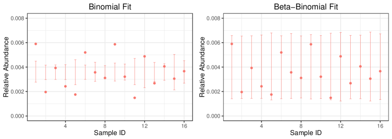
Figure 1: The relative abundance of a strain of Rhizobium in 16 biological replicate samples in a soil microbiology study, and 95% prediction intervals based on a binomial model (left) and the proposed beta-binomial model (right). The data is clearly overdispersed relative to the binomial model, motivating the development of our beta-binomial model.

The overdispersion of the observed relative abundances compared to a binomial model motivates a more flexible model. We propose the following model:

$$W_{i}|(Z_{i},M_{i}) \sim\text{Binomial}(M_{i},Z_{i}),$$ (3.2)

$$Z_{i} \sim\text{Beta}(a_{1,i},a_{2,i}),$$ (3.3)

where $a_{1,i}\in\mathbb{R}_{+}$, $a_{2,i}\in\mathbb{R}_{+}$. In the model (3.2)–(3.3), $Z_{i}$ is itself a random variable, representing the latent relative abundance of the taxon. As we will demonstrate, this hierarchical approach to to modeling relative abundance is a major advantage of our approach.

Using the parameterization

$$\mu_{i} =\frac{a_{1,i}}{a_{1,i}+a_{2,i}},$$ (3.4)

it can be shown that

$$\mathbb{E}(W_{i}|M_{i}) =M_{i}\times\mathbb{E}(Z_{i})=M_{i}\times\mu_{i}.$$ (3.5)

Thus $\mu_{i}\in(0,1)$ is the expected relative abundance of the taxon in the $i^{\text{th}}$ sample. In addition, using the parameterization

$$\phi_{i} =\frac{1}{a_{1,i}+a_{2,i}+1},$$ (3.6)

it can be shown that

$$\text{Var}(W_{i}|M_{i}) =M_{i}\times\mu_{i}\times(1-\mu_{i})\times(1+(M_{i}-1)\times\phi_{i}).$$ (3.7)

The multiplicative factor $(1+(M_{i}-1)\times\phi_{i})$ is therefore the overdispersion of the absolute abundance of the taxon for the $i^{\text{th}}$ sample relative to a binomial random variable. Furthermore,

$$\text{Corr}(Y_{i,j},Y_{i,j^{*}}) =\phi_{i}\text{ for }1\leq j<j^{*}\leq M_{i},$$ (3.8)

so $\phi_{i}$ can also be interpreted as the correlation between the taxon indicator variables within the $i^{\text{th}}$ sample (Prentice, 1986).

We then link the expected relative abundance, $\mu_{i}$, and the overdispersion, $\phi_{i}$, to covariates. We define link functions

$$g(\mu_{i}) =\beta_{0}+\bm{X}_{i}^{T}\bm{\beta},$$ (3.9)

$$h(\phi_{i}) =\beta_{0}^{*}+\bm{X}^{*T}_{i}\bm{\beta}^{*},$$ (3.10)

where $\bm{X}_{i}$, the $i^{\text{th}}$ row of the covariate matrix $\bm{X}=[X_{ij}]\in\mathbb{R}^{n\times k}$, represents covariates associated with $\mu_{i}$; $\bm{X}_{i}^{*}$, the $i^{\text{th}}$ row of the covariate matrix $\bm{X}^{*}=[X^{*}_{ij}]\in\mathbb{R}^{n\times k^{*}}$, represents covariates associated with $\phi_{i}$; $\bm{\beta}=(\beta_{1},\ldots,\beta_{k})^{T}$; and $\bm{\beta}^{*}=(\beta^{*}_{1},\ldots,\beta_{k^{*}}^{*})^{T}$. $\bm{X}$ and $\bm{X}^{*}$ may be identical, or they may be non- or partially-overlapping.

Throughout this paper, we choose the logit transformation for the link functions in (3.9) and (3.10), so that

$$g(x)\equiv h(x) \vcentcolon=\log\left(\dfrac{x}{1-x}\right).$$

This link function is convenient as it is a bijection between $[0,1]$ and $\mathbb{R}$. Other choices for the link functions can be used as well, and the link functions for $\mu_{i}$ and $\phi_{i}$ need not be identical.

This hierarchical model has three key advantages over other approaches. Firstly, the use of a beta random variable as a model for the binomial probability allows us to incorporate overdispersion. Secondly, the overdispersion parameter (rather than just the mean) can be modeled with covariates. As we will see in Section 6, this is a key advantage of our approach. Finally, our model makes direct use of the absolute abundance ($W_{1},\ldots,W_{n}$) and the total number of counts ($M_{1},\ldots,M_{n}$), rather than simply transforming these quantities into the observed relative abundance ($W_{1}/M_{1},\ldots,W_{n}/M_{n}$), which would amount to throwing away valuable information about the sequencing depth across in each sample. We show the 95% prediction intervals from a beta-binomial model for the soil microbiology study in Figure 1 (right).

3.2 Model Fitting

Given $n$ samples from the model (3.2)–(3.3), the log-likelihood is

$$\log L(\bm{\theta}|\bm{W},\bm{M})$$ (3.11)

$$\hskip 5.0pt=\sum_{i=1}^{n}\log\left[\begin{pmatrix}M_{i}\\ W_{i}\end{pmatrix}\frac{B(a_{1,i}+W_{i},\ a_{2,i}+M_{i}-W_{i})}{B(a_{1,i},\ a_{2,i})}\right]$$

$$\hskip 5.0pt=\sum_{i=1}^{n}\log\left[\begin{pmatrix}M_{i}\\ W_{i}\end{pmatrix}\frac{B\left(\dfrac{e^{-\beta_{0}^{*}-\bm{X}_{i}^{*T}\bm{\beta}^{*}}}{1+e^{-\beta_{0}-\bm{X}_{i}^{T}\bm{\beta}}}+W_{i},\ \dfrac{e^{-\beta_{0}^{*}-\bm{X}_{i}^{*T}\bm{\beta}^{*}}}{1+e^{\beta_{0}+\bm{X}_{i}^{T}\bm{\beta}}}+M_{i}-W_{i}\right)}{B\left(\dfrac{e^{-\beta_{0}^{*}-\bm{X}_{i}^{*T}\bm{\beta}^{*}}}{1+e^{-\beta_{0}-\bm{X}_{i}^{T}\bm{\beta}}},\ \dfrac{e^{-\beta_{0}^{*}-\bm{X}_{i}^{*T}\bm{\beta}^{*}}}{1+e^{\beta_{0}+\bm{X}_{i}^{T}\bm{\beta}}}\right)}\right],$$

where $\bm{W}\in\mathbb{R}^{n}$, $\bm{M}\in\mathbb{R}^{n}$, $\bm{\beta}\in\mathbb{R}^{k}$, $\bm{\beta}^{*}\in\mathbb{R}^{k^{*}}$, $\bm{\theta}=(\beta_{0},\bm{\beta}^{T},\beta_{0}^{*},\bm{\beta}^{*T})^{T}$, and $B(\cdot,\cdot)$ is the Beta function given by $B(x,y)=\int_{0}^{1}t^{x-1}(1-t)^{y-1}dt$ for $x\in\mathbb{R}$ and $y\in\mathbb{R}_{+}$. We fit the model by maximum likelihood using the trust region optimization algorithm (Fletcher, 1987; Nocedal and Wright, 1999; Geyer, 2015), which has accelerated computation relative to a line search method.

In this iterative algorithm, a “trust region” is defined around the parameter estimate at each iteration. The algorithm then updates the parameter estimate by minimizing a second-order Taylor series expansion of the objective function, subject to the constraint that the solution is within the trust region. If a proposed update is infeasible (i.e. it is outside of the parameter space), then it is rejected and the trust region shrinks. The minimization of the objective function then repeats with the new constraint. If a proposed update is close to the boundary of the trust region, the trust region expands in the next iteration. We implement the trust algorithm for minimizing the negative log-likelihood using the R package trust (Geyer, 2015).

The log-likelihood is not concave in $\bm{\theta}$ (see Appendix B), so trust region optimization does not guarantee convergence to the global minimum of the objective function. However, under mild conditions, the limit points of the trust algorithm are guaranteed to satisfy the first- and second-order conditions that are necessary for a local minimum (Fletcher, 1987; Nocedal and Wright, 1999). We use multiple initializations and select the estimate that has the largest log-likelihood. In practice, there is little difference in the parameter estimates across initializations.

Each iteration of the trust region optimization algorithm makes use of the gradient and Hessian of (3.11). These are given in Appendix A for the case of logit link functions for $g(\cdot)$ and $h(\cdot)$ in (3.9) and (3.10).

4 Hypothesis Testing

We now discuss inference on $\bm{\theta}$. We consider the null hypothesis that $\bm{A}\bm{\theta}=\bm{b}$, where $\bm{A}\in\mathbb{R}^{r\times(k+k^{*}+2)}$ has full row rank and $r<k+k^{*}+2$, $\bm{b}\in\mathbb{R}^{r}$, and where $\bm{\theta}$ is the parameter vector introduced in (3.11). The Wald test statistic is

$$\hat{T}_{Wald}=n(\bm{A}\hat{\bm{\theta}}-\bm{b})^{T}(\bm{A}\hat{\mathcal{I}}(\hat{\bm{\theta}})_{n}^{-1}\bm{A}^{T})^{-1}(\bm{A}\hat{\bm{\theta}}-\bm{b}),$$ (4.1)

where

$$\hat{\bm{\theta}}=\operatornamewithlimits{argsup}_{\bm{\theta}}\log L(\bm{\theta}|\bm{W},\bm{M})$$ (4.2)

and $\hat{\mathcal{I}}(\hat{\bm{\theta}})_{n}$ is the observed Fisher information evaluated at $\hat{\bm{\theta}}$:

$$\hat{\mathcal{I}}(\hat{\bm{\theta}})_{n}=-\dfrac{1}{n}\sum_{i=1}^{n}\left[\dfrac{\partial^{2}}{\partial\bm{\theta}\partial\bm{\theta}^{T}}\log L(\bm{\theta}|\bm{W},\bm{M})\right]_{\bm{\theta}=\hat{\bm{\theta}}}.$$ (4.3)

Under the null hypothesis that $\bm{A}\bm{\theta}=\bm{b}$, we find empirically that $\hat{T}_{Wald}$ is well-approximated by a $\chi^{2}_{r}$ distribution if $n$ is large (Section 5.1). Alternatively, we can test $\bm{A}\bm{\theta}=\bm{b}$ using a likelihood ratio test statistic, defined as

$$\hat{T}_{LRT}=2\left(\log L(\hat{\bm{\theta}}|\bm{W},\bm{M})-\log L(\hat{\bm{\theta}}_{0}|\bm{W},\bm{M})\right),$$ (4.4)

where

$$\hat{\bm{\theta}}_{0}=\operatornamewithlimits{argsup}_{\bm{\theta}:\bm{A}\bm{\theta}=\bm{b}}\log L(\bm{\theta}|\bm{W},\bm{M}).$$ (4.5)

When $n$ is large and $\bm{A}\bm{\theta}=\bm{b}$, we find that the distribution of $\hat{T}_{LRT}$ is well-approximated by a $\chi^{2}_{r}$ distribution (Section 5.1).

In practice, we often do not have the sample size necessary to use the $\chi^{2}_{r}$ approximation. For this reason, we also implement a parametric bootstrap hypothesis testing procedure. Our parametric bootstrap Wald testing procedure is given in Algorithm 1; the parametric bootstrap likelihood ratio test procedure is provided in Appendix C.

Require: $\bm{W}$, $\bm{M}$, $\bm{X}$, $\bm{X}^{*}$, a large integer $B$ (e.g. $B=10,000$)

1:Estimate $\hat{\bm{\theta}}$ and $\hat{\bm{\theta}}_{0}$ as in (4.2) and (4.5), respectively, with the trust region optimization procedure.

2:Compute $\hat{T}_{Wald}$ as in (4.1) using $\bm{A}$, $\bm{b}$, and $\hat{\bm{\theta}}$.

3:for $b=1,\ldots,B$ do

4:     Simulate $\tilde{\bm{W}}^{b}$ with elements $\tilde{W}_{i}^{b}$ drawn from a beta-binomial distribution with $M_{i}$      draws and parameters $\hat{\bm{\theta}}_{0}$.

5:     Estimate $\tilde{\bm{\theta}}^{b}$ as in (4.2) using $\tilde{\bm{W}}^{b}$ and $\bm{M}$ with the trust region optimization procedure.

6:     Compute $\hat{T}^{b}_{Wald}$ as in (4.1) using $\bm{A}$, $\bm{b}$, and $\tilde{\bm{\theta}}^{b}$.

7:Calculate the p-value:

$$\hat{p}\leftarrow\dfrac{1}{B+1}\left(1+\sum_{b=1}^{B}\mathbbm{1}\left\{\hat{T}^{b}_{Wald}\geq\hat{T}_{Wald}\right\}\right).$$

8:return $\hat{p}$

Algorithm 1 Parametric Bootstrap Wald Test of $H_{0}:\ \bm{A}\bm{\theta}=\bm{b}$

For certain realizations of $\bm{W}$, Wald-type inference is uninformative. For example, if $k=k^{*}=1$, $\bm{X}_{i}=\bm{X}_{i}^{*}\in\left\{0,\ 1\right\}$ for $i=1,\ldots,n$, and $\sum_{i:\ \bm{X}_{i}=1}W_{i}=0$, then a parameter estimate diverges to $-\infty$ (see Lemma D.1 in Appendix D for details). This limitation is not unique to our model, and hypothesis testing using Wald tests in the case of complete or quasi-complete separation in logistic regression is known to have the same issue (see Albert and Anderson (1984); Heinze and Schemper (2002); Heinze (2006) for further discussion). In this case, we instead use the likelihood ratio test to test hypotheses about $\bm{\beta}$, such as $\bm{\beta}=0$. However, in this setting, even the likelihood ratio test does not provide a useful test of certain hypotheses about $\bm{\beta}^{*}$, such as $\bm{\beta}^{*}=0$ (see Appendix D). Since it is often the case that a taxon is unobserved in certain experimental conditions, the default behaviour for our software in this setting is to return a test statistic of zero for Wald-type tests to indicate that inference is uninformative and the null hypothesis should not be rejected.

While (4.4) and Algorithms 1–2 hold for any $\bm{A}$ and $\bm{b}$, they require solving (4.5). This may be difficult to do for certain $\bm{A}$ and $\bm{b}$. In this case, an approximate solution could be obtained by maximizing the likelihood subject to a penalty on $\left\lVert\bm{A}\bm{\theta}-\bm{b}\right\rVert$ (e.g. see Fiacco and McCormick (1968); Ryan (1974)). Alternatively, approximating the distribution of (4.1) with a $\chi^{2}_{r}$ distribution does not require restricted maximum likelihood estimation.

In summary, we implement four hypothesis testing procedures: the Wald test, the likelihood ratio test, the parametric bootstrap Wald test, and the parametric bootstrap likelihood ratio test. The Wald and likelihood ratio tests permit faster inference than the parametric bootstrap tests. However, the parametric bootstrap procedures successfully control Type 1 error in small sample sizes. We now demonstrate the performance of all of these hypothesis testing procedures in simulation.

5 Simulation Study

We now investigate the performance of our approach, which we call count regression for correlated observations with the beta-binomial, or corncob, under simulation. We study the Type I error rate and the power when testing for both differential abundance and differential variability. We generate sequencing depths $\bm{M}\in\mathbb{R}^{n}$ with elements $M_{i}$ simulated from the empirical distribution of the observed sequencing depths in the data set discussed in Section 6, which ranges from $7,821$ to $58,655$. We use sample sizes $n\in\left\{10,30,100\right\}$ and a binary covariate $\bm{X}_{i}=\bm{X}_{i}^{*}=0$ for $i=1,\ldots,n/2-1$ and $\bm{X}_{i}=\bm{X}_{i}^{*}=1$ for $i=n/2,\ldots,n$. We then simulate absolute abundances $\bm{W}\in\mathbb{R}^{n}$ with elements $W_{i}$ simulated under the data generating model (described below). The parameter values were selected by fitting corncob to the genus Thermomonas in the data set discussed in Section 6 so that simulated data are similar to what might be observed in a real-world experiment. For each simulation, we calculate $10,000$ p-values using all four of the hypothesis testing procedures outlined in Section 4: the Wald test, the likelihood ratio test, the parametric bootstrap Wald test, and the parametric bootstrap likelihood ratio test. We use $1,000$ bootstrap iterations for the parametric bootstrap testing procedures.

5.1 Type I Error Rate

We first confirm that corncob controls Type I error at the nominal level. We generate data using the beta-binomial model with logit link functions for mean and overdispersion, under three settings for $\bm{\beta}$. In the first simulation setting, we test the null hypothesis $H_{0}:(\beta_{1},\beta_{1}^{*})=(0,0)$. We generated model parameters by fitting a model to the genus Thermomonas without using soil amendment as a covariate, yielding parameters $(\tilde{\beta}_{0},\tilde{\beta}_{1},\tilde{\beta}_{0}^{*},\tilde{\beta}_{1}^{*})=(-5.75,0,-5.24,0)$. In the second simulation setting, we test the null hypothesis $H_{0}:\beta_{1}^{*}=0$. We generated model parameters by fitting a model to the genus Thermomonas using soil amendment as a covariate for $\mu_{i}$, yielding parameters $(\tilde{\beta}_{0},\tilde{\beta}_{1},\tilde{\beta}_{0}^{*},\tilde{\beta}_{1}^{*})=(-5.36,-1.12,-5.69,0)$. In the third simulation setting, we test the null hypothesis $H_{0}:\beta_{1}=0$. We generated model parameters by fitting a model to the genus Thermomonas using soil amendment as a covariate for $\phi_{i}$, yielding parameters $(\tilde{\beta}_{0},\tilde{\beta}_{1},\tilde{\beta}_{0}^{*},\tilde{\beta}_{1}^{*})=(-5.51,0,-5.38,0.70)$. For all three simulation settings, the null hypotheses are true, so we would expect p-values obtained from testing the null hypotheses to be uniformly distributed.

The results are shown in Figure 2. For sample sizes of $30$ and $100$, all testing procedures resulted in approximately uniform p-values, and Type I error is controlled. This suggests that for this experiment, a sample size of $30$ is sufficient to approximate the distribution of the Wald and likelihood ratio test statistics using a $\chi^{2}$ distribution.

For a sample size of $10$, only the parametric bootstrap procedures resulted in approximately uniform p-values and successful Type I error control. The p-values obtained using the Wald and likelihood ratio tests were anti-conservative, suggesting that for this experiment, a sample size of $10$ is too small to approximate the distribution of the test statistics using a $\chi^{2}$ distribution. Therefore, to obtain reliable inference, we recommend the parametric bootstrap procedure when $n$ is smaller than $30$.

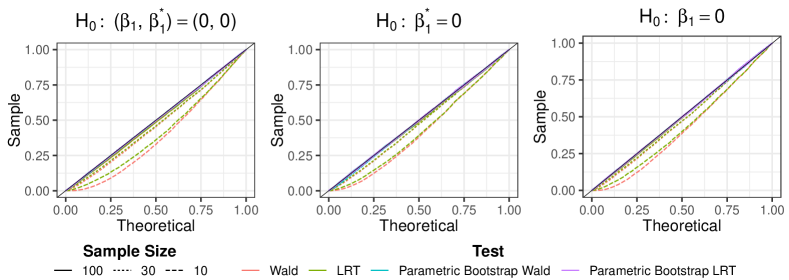
Figure 2: Quantiles of p-values obtained from the Type I error rate simulation settings compared to quantiles of a Uniform$(0,1)$ distribution. We test the null hypotheses $H_{0}:(\beta_{1},\beta_{1}^{*})=(0,0)$ (left), $H_{0}:\beta_{1}^{*}=0$ (middle), and $H_{0}:\beta_{1}=0$ (right). A 45-degree line is shown (black). P-values were obtained using Wald (red), likelihood ratio (green), parametric bootstrap Wald (blue), and parametric bootstrap likelihood ratio (purple) tests. Sample sizes used were 10 (dashed), 30 (dotted), and 100 (solid).

5.2 Power

We now investigate the power of corncob to reject (i) the null hypothesis $H_{0}:\ \beta_{1}=0$, as well as (ii) the null hypothesis $H_{0}:\ \beta_{1}^{*}=0$. We consider two cases: varying the value of $\beta_{1}$, and varying the value of $\beta_{1}^{*}$. For both settings, we generated model parameters by fitting a model to the genus Thermomonas using soil amendment as a covariate for $\mu_{i}$ and $\phi_{i}$, yielding parameters $(\tilde{\beta}_{0},\tilde{\beta}_{1},\tilde{\beta}_{0}^{*},\tilde{\beta}_{1}^{*})=(-5.17,-2.46,-5.13,-3.88)$. In the first case (Setting 4 in Figure 3), we set $(\beta_{0},\beta_{1},\beta_{0}^{*},\beta_{1}^{*})=(\tilde{\beta}_{0},c\tilde{\beta}_{1},\tilde{\beta}_{0}^{*},\tilde{\beta}_{1}^{*})$ using $c\in\left\{0,0.05,\ldots,1\right\}$. In the second case (Setting 5 in Figure 3), we set $(\beta_{0},\beta_{1},\beta_{0}^{*},\beta_{1}^{*})=(\tilde{\beta}_{0},\tilde{\beta}_{1},\tilde{\beta}_{0}^{*},c\tilde{\beta}_{1}^{*})$ using $c\in\left\{0,0.05,\ldots,1\right\}$.

The results of the power analyses are shown in Figure 3. For both null hypotheses, all sample sizes, and all hypothesis testing procedures, the power increases as both the sample size and the magnitude of the coefficient being tested increases. For sample sizes of $30$ and $100$, there is little difference in power across the four testing procedures. This is not surprising, given that in the simulations in Section 5.1, all procedures performed similarly with sample sizes of $30$ and $100$. We do not show results for the procedures that rely on the asymptotic distribution of the test statistics for $n=10$, as we saw in Section 5.1 that these procedures did not properly control Type I error.

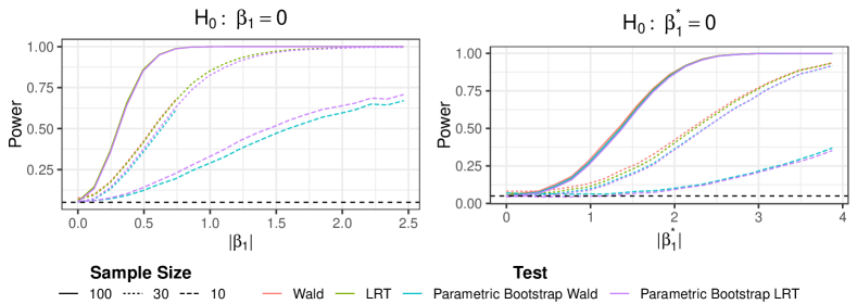
Figure 3: Power curves of p-values obtained from the power simulations. Setting 4 (left) tests $H_{0}:\beta_{1}=0$. Setting 5 (right) tests $H_{0}:\beta_{1}^{*}=0$. A horizontal dashed line is shown at $0.05$. P-values were obtained using Wald (red), likelihood ratio (green), parametric bootstrap Wald (blue), and parametric bootstrap likelihood ratio (purple) tests. Sample sizes used were 10 (dashed), 30 (dotted), and 100 (solid).

6 Application to Soil Data

We now consider a study of the association between soil treatments and soil microbiome composition (Whitman and others, 2016). In this experiment, there are three groups of soil treatments: no additions, biochar additions, and fresh biomass additions. For each treatment group, multiple experimental replicates were taken at three time points: on the first day, after 12 days, and after 82 days. The data include $n=119$ samples with sequencing depths ranging from $8,830$ to $194,356$. After quality control (as described in Whitman and others (2016)), a total of $7,770$ operational taxonomic units were identified using the UPARSE workflow (Edgar, 2013), and taxonomy was assigned using reference databases. Using the assigned taxonomy, we aggregated counts to the genus level, giving $241$ genera.

We are interested in applying our method to compare the microbiome of soil with no additions after 82 days $(n=15)$ to the microbiome of soil with biochar additions after 82 days $(n=16)$. We remove $13$ genera for which the total number of counts in these $31$ samples is zero. We apply corncob using soil addition as a covariate for $\mu_{i}$ and $\phi_{i}$ as in (3.9) and (3.10). We calculate p-values using the parametric bootstrap likelihood ratio test (Algorithm 2) with $B=10^{6}$ bootstrap iterations. We compare the results of corncob to those from DESeq2 (Love and others, 2014), EdgeR (Robinson and others, 2010), metagenomeSeq (Paulson and others, 2013), and a zero-inflated beta (ZIB) regression model (Peng and others, 2016).

6.1 Detection of Differential Abundance

We first compare p-values obtained from testing for differential abundance across soil addition group. Roughly speaking, each of the approaches tests for a difference in abundance of a single taxon across conditions, although the details of the model used vary across methods. In the context of corncob, testing for differential abundance amounts to testing the null hypothesis $H_{0}:\ \bm{\beta}=0$, using the notation defined in (3.9). Scatter plots of the negative log-10 p-values for each approach are shown in Figure 4.

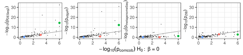
Figure 4: The negative log-10 p-values obtained by testing for differential abundance using corncob ($H_{0}:\bm{\beta}=0$) compared to those from DESeq2 (left-most, Spearman’s correlation coefficient $\rho=0.854$), EdgeR (middle-left, $\rho=0.783$), metagenomeSeq (middle-right, $\rho=0.552$), and ZIB (right-most, $\rho=0.705$). A 45-degree line is shown. We see that the p-values are on a similar scale overall. Thermomonas (green), Flavisolibacter (red), and Myxococcus (blue) are further examined in Figure 6.

Overall, as p-values calculated using corncob decrease, so do those calculated using other approaches. We observe moderate to strong correlations across the different approaches, with Spearman’s correlation coefficients between the p-values obtained from corncob ($H_{0}:\ \bm{\beta}=0$) and DESeq2, edgeR, metagenomeSeq, and ZIB, respectively, of 0.854, 0.783, 0.552, 0.705. corncob calculated a lower p-value for 53.9%, 43.6%, 63.8%, and 58.3% of genera compared to DESeq2, edgeR, metagenomeSeq, and ZIB, respectively. Median p-values across all genera for corncob, DESeq2, edgeR, metagenomeSeq, and ZIB are 0.273, 0.318, 0.297, 0.491, and 0.320, respectively. Therefore, while the p-values produced by corncob are on a similar scale to the other approaches, they may be higher or lower for any given taxon. While each of the approaches uses a different model and makes use of a different test statistic, they are all testing for some difference in the mean abundance of the taxon across the soil addition. Thus, it is unsurprising that the p-values are similar across the approaches.

6.2 Detection of Differential Variability

We now test for differences in the variability of the abundance of a single taxon across conditions, which we refer to as differential variability. Using corncob and the notation in (3.9)–(3.10), this amounts to testing the null hypothesis $H_{0}:\ \bm{\beta}^{*}=0$. As far as we know, corncob is the only approach that explicitly tests for differential variability. Thus, in this section, we investigate whether testing for differential variability allows us to identify new genera beyond what we identify when testing only for differential abundance.

We compare the results of testing for differential variability to the results of testing for differential abundance using the methods investigated in Section 6.1. Figure 5 shows scatter plots of the negative log-10 transformations of the p-values for testing differential abundance from DESeq2, metagenomeSeq, ZIB, and corncob against the p-values for testing differential variability with corncob. We see from Figure 5 that there is only a weak association between the p-values for differential variability obtained using corncob and the p-values for differential abundance obtained using the other approaches. In particular, Spearman’s correlation coefficients are 0.127, 0.234, 0.132, 0.215, and 0.362 between corncob p-values for $H_{0}:\ \bm{\beta}^{*}=0$ and p-values from DESeq2, edgeR, metagenomeSeq, ZIB, and corncob for $H_{0}:\ \bm{\beta}=0$, respectively. We omit from Figure 5 the scatter plot comparing the corncob p-values for $H_{0}:\ \bm{\beta}^{*}=0$ to the edgeR p-values because the p-values from edgeR are similar to those from DESeq2. We conclude that applying corncob to test $H_{0}:\ \bm{\beta}^{*}=0$ leads to the discovery of a very different set of genera than those discovered by applying corncob or other approaches to test for differential abundance.

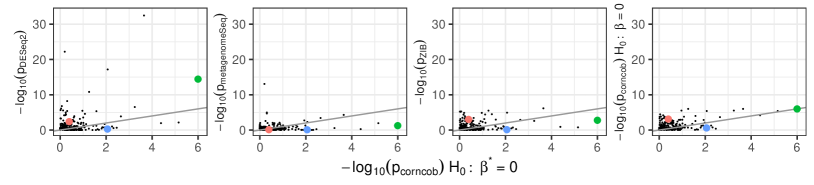
Figure 5: The negative log-10 p-values obtained by testing for differential variability using corncob ($H_{0}:\ \bm{\beta}^{*}=0$) compared to the negative log-10 p-values obtained by testing for differential abundance using DESeq2 (left-most, Spearman’s correlation coefficient $\rho=0.127$), metagenomeSeq (middle-left, $\rho=0.132$), ZIB (middle-right, $\rho=0.215$), and corncob ($H_{0}:\ \bm{\beta}=0$) (right-most, $\rho=0.362$). A 45-degree line is shown. Thermomonas (green), Flavisolibacter (red), and Myxococcus (blue) are further examined in Figure 6. We omit a scatter plot showing p-values for edgeR ($\rho=0.234$); results are similar to DESeq2.

To obtain greater insight into the results shown in Figure 5, we consider the 3 highlighted genera, which we further investigate in Figure 6. The first, Thermomonas, has small p-values for both differential abundance ($p=1.00\times 10^{-6}$) and differential variability ($p=1.00\times 10^{-6}$) using corncob. The second, Flavisolibacter, has a small p-value for differential abundance ($p=7.44\times 10^{-4}$) and a large p-value for differential variability ($p=0.404$). The third, Myxococcus, has a large p-value for differential abundance ($p=0.244$) and a small p-value for differential variability ($p=8.83\times 10^{-3}$), so it would not be identified using the competing approaches (see Figure 6 for p-values from all approaches). Figure 6 indicates a clear visual difference between genera that are identified as differentially abundant but not differentially variable, differentially variable but not differentially abundant, and both differentially abundant and differentially variable. Researchers can use corncob to distinguish between these three possibilities.

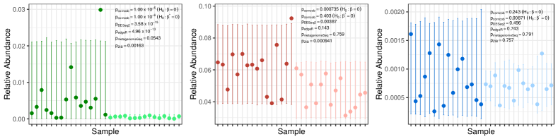
Figure 6: The observed relative abundances of the genera Thermomonas (left), Flavisolibacter (middle), and Myxococcus (right) in 31 soil samples. Each of these genera is highlighted in each panel of Figures 4 and 5. In each panel, the first 16 samples correspond to the biochar additions group (darker color), and the remaining 15 samples correspond to the no additions group (lighter color). 95% prediction intervals for the relative abundances from a corncob fit using soil addition as a covariate for $\mu_{i}$ and $\phi_{i}$ are shown. Using corncob to test $H_{0}:\ \bm{\beta}=0$ and $H_{0}:\ \bm{\beta}^{*}=0$ indicates that Thermomonas is both differentially abundant ($p=1.00\times 10^{-6}$) and differentially variable ($p=1.00\times 10^{-6}$), Flavisolibacter is differentially abundant ($p=7.44\times 10^{-4}$) and not differentially variable ($p=0.404$), and Myxococcus is differentially variable ($p=8.83\times 10^{-3}$) and not differentially abundant ($p=0.244$).

In practice, a data analyst will apply a multiple testing procedure to adjust the p-values for multiple comparisons, so we also investigative the number of genera identified as either differentially abundant or differentially variable after applying the Benjamini-Hochberg procedure (Benjamini and Hochberg, 1995) to the p-values obtained using corncob to test $H_{0}:\ \bm{\beta}=0$ and $H_{0}:\ \bm{\beta}^{*}=0$. The results are shown in Figure 7. We see that for a given false discovery rate, in this data set we detect more genera as being differentially abundant than differentially variable; this can also be seen in the right-most panel of Figure 5. All code for performing this analysis is available in the supplementary materials available at github.com/bryandmartin/corncob_supplementary.

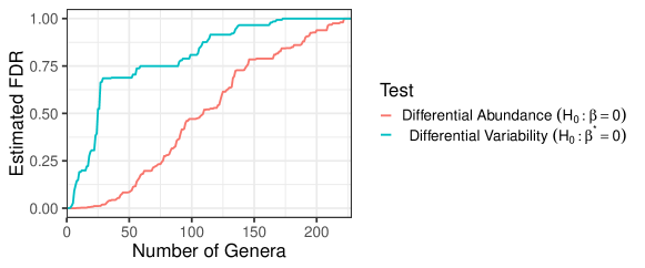
Figure 7: The estimated false discovery rate using the Benjamini-Hochberg procedure, as a function of the number of genera identified as differentially abundant and differentially variable. For a given false discovery rate, we identify fewer genera that are differentially variable than differentially abundant.

7 Discussion

In this paper, we have proposed a beta-binomial regression model for abundance data. Our model extends existing beta-binomial models by allowing discrete and continuous covariates to be linked to both a relative abundance parameter and an overdispersion parameter. Our method is particularly well-suited to modeling microbial abundance data for a number of reasons. First, microbial taxa are commonly unobserved in many samples. For example, in the data set examined in Section 6, 34% of absolute abundances were zero. Our model can accommodate this without requiring a zero-inflation component or pseudo-counts. Second, studies of microbial populations often have small sample sizes. Our simulation study in Section 5 suggests that our parametric bootstrap inference methods (Algorithms 1 and 2) give valid inference even with small samples. Third, the interpretation of $\mu_{i}$ as the expected relative abundance and of $\phi_{i}$ as the within-sample correlation of taxon labels (i.e. $\phi_{i}=\text{Corr}(Y_{ij}=Y_{ij^{\prime}})$, see Section 3) are intuitive and complement ecological theory (Welch and others, 2016). Finally, regression models for contrasting microbial populations commonly focus on differential abundance. By conducting inference about $\phi_{i}$, our model is also able to identify differences in microbial populations associated with differential variability.

Many studies (e.g. see Gerber (2014); Faust and others (2015); Zhou and others (2015), among others) employ a longitudinal design to investigate the dynamics of microbial populations over time. To accommodate this setting, future work could incorporate random effects into (3.9) and (3.10).

Our proposed approach models a single taxon’s abundance. A limitation of this approach is that it does not enforce the compositionality constraint (i.e. the estimated expected relative abundances need not sum to $1$ across all microbes in the population). Future work could consider a multivariate extension of our approach to enforce the compositionality constraint or incorporate between-taxon correlations.

All methods proposed in this paper are implemented in an R package available at github.com/bryandmartin/corncob. Code to reproduce all simulations and data analyses are available at github.com/bryandmartin/corncob_supplementary.

Appendix A Analytic Expressions for the Gradient and Hessian

Let $\gamma_{i}=\frac{\phi_{i}}{1-\phi_{i}}$ for all $i$, and define $\psi(x)=\int_{0}^{\infty}\left(\frac{e^{-t}}{t}-\frac{e^{-xt}}{1-e^{-t}}\right)dt$ for $x\in\mathbb{R}_{+}$ to be the digamma function, the derivative of the logarithm of the gamma function. Define $\bm{Z}_{i}=\begin{pmatrix}1&\bm{X}_{i}\end{pmatrix}$ and $\bm{Z}_{i}^{*}=\begin{pmatrix}1&\bm{X}_{i}^{*}\end{pmatrix}$ to be the design matrices for covariates associated with $\mu_{i}$ and $\phi_{i}$, respectively, including intercept terms. Then the expression for the gradient of (3.11) is given by

$$\dfrac{\partial\log L(\bm{\theta}|\bm{W},\bm{M})}{\partial\bm{\beta}} =\sum_{i=1}^{n}\bigg{\{}\gamma_{i}^{-1}\mu_{i}(1-\mu_{i})\mathbf{Z}_{i}\bigg{[}\psi\left(\dfrac{1-\mu_{i}}{\gamma_{i}}\right)$$ (A.1)

$$\hskip 20.00003pt-\psi\left(M_{i}+\dfrac{1-\mu_{i}-W_{i}\gamma_{i}}{\gamma_{i}}\right)$$

$$\hskip 20.00003pt+\psi\left(W_{i}+\dfrac{\mu_{i}}{\gamma_{i}}\right)-\psi\left(\dfrac{\mu_{i}}{\gamma_{i}}\right)\bigg{]}\bigg{\}},$$

$$\dfrac{\partial\log L(\bm{\theta}|\bm{W},\bm{M})}{\partial\bm{\beta}^{*}} =\sum_{i=1}^{n}\bigg{\{}\gamma_{i}^{-1}\mathbf{Z}^{*}_{i}\bigg{[}\psi\left(M_{i}+\dfrac{1}{\gamma_{i}}\right)-\psi\left(\dfrac{1}{\gamma_{i}}\right)+(\mu_{i}-1)$$ (A.2)

$$\hskip 20.00003pt\bigg{(}\psi\left(M_{i}+\dfrac{1-\mu_{i}-W_{i}\gamma_{i}}{\gamma_{i}}\right)-\psi\left(\dfrac{1-\mu_{i}}{\gamma_{i}}\right)\bigg{)}$$

$$\hskip 20.00003pt+\mu_{i}\left(\psi\left(\dfrac{\mu_{i}}{\gamma_{i}}\right)-\psi\left(W_{i}+\dfrac{\mu_{i}}{\gamma_{i}}\right)\right)\bigg{]}\bigg{\}}.$$

Let $\psi^{(1)}(x)=\dfrac{\partial}{\partial x}\psi(x)$ be the trigamma function. Define $\bm{Y}_{i}=\begin{pmatrix}\bm{Z}_{i}^{T}&\bm{0}\end{pmatrix}^{T}\in\mathbb{R}^{k+k^{*}+2}$ and $\bm{Y}_{i}^{*}=\begin{pmatrix}\bm{0}&\bm{Z}_{i}^{*T}\end{pmatrix}^{T}\in\mathbb{R}^{k+k^{*}+2}$. Then the expression for the Hessian of (3.11), $\bm{H}$, is given by

$$\bm{H}=\sum_{i=1}^{n} \bigg{[}c_{1,i}\mu_{i}^{2}(1-\mu_{i})^{2}\bm{Y}_{i}\bm{Y}_{i}^{T}+c_{2,i}\left(\mu_{i}(1-\mu_{i})\bm{Y}_{i}\gamma_{i}\bm{Y}_{i}^{*T}\right.$$

$$\hskip 20.00003pt\left.+\gamma_{i}\bm{Y}_{i}^{*}\mu_{i}(1-\mu_{i})\bm{Y}_{i}^{T}\right)+c_{3,i}\left(\gamma_{i}\bm{Y}_{i}^{*}\gamma_{i}\bm{Y}_{i}^{*T}\right)$$

$$\hskip 20.00003pt+c_{4,i}\left(\mu_{i}(1-\mu_{i})(1-2\mu_{i})\bm{Y}_{i}\bm{Y}_{i}^{T}\right)+c_{5,i}\left(\gamma_{i}\bm{Y}_{i}^{*}\bm{Y}_{i}^{*T}\right)\bigg{]},$$

where

$$c_{1,i} =\Big{[}\psi^{(1)}\left(M_{i}+(1-\mu_{i}-W_{i}\gamma_{i})/\gamma_{i}\right)-\psi^{(1)}\left((1-\mu_{i})/\gamma_{i}\right)$$

$$\hskip 20.00003pt+\psi^{(1)}\left(W_{i}+\mu_{i}/\gamma_{i}\right)-\psi^{(1)}\left(\mu_{i}/\gamma_{i}\right)\Big{]}\gamma_{i}^{-2},$$

$$c_{2,i} =\Big{[}\gamma_{i}(\psi(M_{i}-(\mu_{i}+W_{i}\gamma_{i}-1)/\gamma_{i})-\psi((1-\mu_{i})/\gamma_{i}))+\gamma_{i}(\psi(\mu_{i}/\gamma_{i})$$

$$\hskip 20.00003pt-\psi(\mu_{i}/\gamma_{i}+W_{i}))+(\mu_{i}-1)(\psi^{(1)}((1-\mu_{i})/\gamma_{i})$$

$$\hskip 20.00003pt-\psi^{(1)}(M_{i}-(\mu_{i}+W_{i}\gamma_{i}-1)/\gamma_{i}))+\psi^{(1)}(\mu_{i}/\gamma_{i})$$

$$\hskip 20.00003pt-\psi^{(1)}(\mu_{i}/\gamma_{i}+W_{i})\Big{]}\gamma_{i}^{-3},$$

$$c_{3,i} =\Big{[}2\gamma_{i}\psi(1/\gamma_{i})+\psi^{(1)}(1/\gamma_{i})-2\gamma_{i}\psi(M_{i}+1/\gamma_{i})-\psi^{(1)}(M_{i}+1/\gamma_{i})$$

$$\hskip 20.00003pt+(\mu_{i}-1)^{2}\psi^{(1)}(M_{i}-(\mu_{i}+W_{i}\gamma_{i}-1)/\gamma_{i})$$

$$\hskip 20.00003pt-2\gamma_{i}(\mu_{i}-1)\psi(M_{i}-(\mu_{i}+W_{i}\gamma_{i}-1)/\gamma_{i})-\mu_{i}^{2}\psi^{(1)}(\mu_{i}/\gamma_{i})$$

$$\hskip 20.00003pt+\mu_{i}^{2}\psi^{(1)}(\mu_{i}/\gamma_{i}+W_{i})-(\mu_{i}-1)^{2}\psi^{(1)}((1-\mu_{i})/\gamma_{i})$$

$$\hskip 20.00003pt+2\gamma_{i}(\mu_{i}-1)\psi((1-\mu_{i})/\gamma_{i})-2\gamma_{i}\mu_{i}\psi(\mu_{i}/\gamma_{i})$$

$$\hskip 20.00003pt+2\gamma_{i}\mu_{i}\psi(\mu_{i}/\gamma_{i}+W_{i})\Big{]}\gamma_{i}^{-4},$$

$$c_{4,i} =\Big{[}\psi((1-\mu_{i})/\gamma_{i})-\psi(M_{i}-(\mu_{i}+W_{i}\gamma_{i}-1)/\gamma_{i})+\psi(\mu_{i}/\gamma_{i}+W_{i})$$

$$\hskip 20.00003pt-\psi(\mu_{i}/\gamma_{i})\Big{]}\gamma_{i}^{-1},$$

$$c_{5,i} =\Big{[}\psi(M_{i}+1/\gamma_{i})-\psi(1/\gamma_{i})+\mu_{i}(\psi(\mu_{i}/\gamma_{i})-\psi(\mu_{i}/\gamma_{i}+W_{i}))$$

$$\hskip 20.00003pt+(\mu_{i}-1)(\psi(M_{i}-(\mu_{i}+W_{i}\gamma_{i}-1)/\gamma_{i})-\psi((1-\mu_{i})/\gamma_{i}))\Big{]}\gamma_{i}^{-2}.$$

Appendix B Non-Concavity of the Beta-Binomial Log-likelihood

We show that (3.11) is not guaranteed to be concave in $\bm{\theta}$. Let $n=1$, $\bm{W}\equiv W_{1}=15$, and $\bm{M}\equiv M_{1}=2000$. Suppose further that $\bm{\theta}=(\beta_{0},\beta_{0}^{*})^{T}$. Let $\bm{\theta}^{1}=\begin{pmatrix}-3&-5\end{pmatrix}^{T}$ and $\bm{\theta}^{2}=\begin{pmatrix}-1&-5\end{pmatrix}^{T}$. Then

$$\log L(\bm{\theta}^{1}|W_{1},M_{1}) =-8.481,$$

$$\log L(\bm{\theta}^{2}|W_{1},M_{1}) =-9.816,$$

$$\log L(0.5\bm{\theta}^{1}+0.5\bm{\theta}^{2}|W_{1},M_{1}) =-9.251.$$

Therefore there exists $\bm{\theta}^{1},$ and $\bm{\theta}^{2}$ such that

$$\log L(0.5\bm{\theta}^{1}+0.5\bm{\theta}^{2}|\bm{W},\bm{M})<0.5\log L(\bm{\theta}^{1}|\bm{W},\bm{M})+0.5\log L(\bm{\theta}^{2}|\bm{W},\bm{M}),$$

which establishes that (3.11) is not concave in $\bm{\theta}$.

Appendix C Parametric Bootstrap Likelihood Ratio Test

We present Algorithm 2 to conduct a parametric bootstrap likelihood ratio test.

Require: $\bm{W}$, $\bm{M}$, $\mathbf{X}$, $\mathbf{X}^{*}$, a large integer $B$ (e.g. $B=10,000$)

1:Estimate $\hat{\bm{\theta}}$ and $\hat{\bm{\theta}}_{0}$ as in (4.2) and (4.5), respectively, with the trust region optimization procedure.

2:Compute $\hat{T}_{LRT}$ as in (4.4) using $\bm{W}$, $\bm{M}$, $\hat{\bm{\theta}}$, and $\hat{\bm{\theta}}_{0}$.

3:for $b=1,\ldots,B$ do

4:     Simulate $\tilde{\bm{W}}^{b}$ with elements $\tilde{W}_{i}^{b}$ drawn from a beta-binomial distribution with $M_{i}$      draws and parameters $\hat{\bm{\theta}}_{0}$.

5:     Estimate $\tilde{\bm{\theta}}^{b}$ as in (4.2) using $\tilde{\bm{W}}^{b}$ and $\bm{M}$ with the trust region optimization procedure.

6:     Estimate $\tilde{\bm{\theta}}_{0}^{b}$ as in (4.5) using $\tilde{\bm{W}}^{b}$ and the trust region optimization procedure.

7:     Compute $\hat{T}^{b}_{LRT}$ as in (4.4) using $\tilde{\bm{W}}^{b}$, $\bm{M}$, $\tilde{\bm{\theta}}^{b}$, and $\tilde{\bm{\theta}}_{0}^{b}$.

8:Calculate the p-value:

$$\hat{p}\leftarrow\dfrac{1}{B+1}\left(1+\sum_{b=1}^{B}\mathbbm{1}\left\{\hat{T}^{b}_{LRT}\geq\hat{T}_{LRT}\right\}\right).$$

9:return $\hat{p}$

Algorithm 2 Parametric Bootstrap Likelihood Ratio Test of $H_{0}:\ \bm{A}\bm{\theta}=\bm{b}$

Appendix D Likelihood Ratio Testing with a Zero-Count Group

We prove that testing the null hypothesis $H_{0}:\ \bm{\beta}^{*}=0$ results in a test statistic of zero under certain conditions. We first prove in Lemma D.1 that the log-likelihood of the model (3.2)–(3.3) is equal to zero under certain conditions. We use this to prove our main claim in Theorem D.2.

Lemma D.1.

Consider the model (3.2)–(3.3) with parameters as in (3.4)–(3.6) and link functions as in (3.9)–(3.10) in the simplified setting with no covariates for $\mu_{i}$, so that $\bm{\theta}=(\beta_{0},\beta_{0}^{*},\bm{\beta}^{*T})^{T}$. Suppose that $\sum_{i}W_{i}=0$. Then

$$\sup_{\beta_{0}}\log L(\bm{\theta}|\bm{W},\bm{M})=0.$$

Proof.

We write the log-likelihood

$$\log L(\bm{\theta}|\bm{W},\bm{M})=\sum_{i=1}^{n}\log\left[\begin{pmatrix}M_{i}\\ W_{i}\end{pmatrix}\frac{B\left(\dfrac{e^{-\beta_{0}^{*}-\bm{X}_{i}^{*T}\bm{\beta}^{*}}}{1+e^{-\beta_{0}}}+W_{i},\ \dfrac{e^{-\beta_{0}^{*}-\bm{X}_{i}^{*T}\bm{\beta}^{*}}}{1+e^{\beta_{0}}}+M_{i}-W_{i}\right)}{B\left(\dfrac{e^{-\beta_{0}^{*}-\bm{X}_{i}^{*T}\bm{\beta}^{*}}}{1+e^{-\beta_{0}}},\ \dfrac{e^{-\beta_{0}^{*}-\bm{X}_{i}^{*T}\bm{\beta}^{*}}}{1+e^{\beta_{0}}}\right)}\right].$$

Substituting $W_{i}=0$, using the definition of $B(\cdot,\cdot)$, and taking the limit in $\beta_{0}$ gives

$$\lim_{\beta_{0}\to-\infty}\log L(\bm{\theta}|\bm{W},\bm{M}) =\lim_{\beta_{0}\to-\infty}\sum_{i=1}^{n}\log\left[\Gamma\left(\dfrac{e^{-\beta_{0}^{*}-\bm{X}_{i}^{*T}\bm{\beta}^{*}}}{1+e^{\beta_{0}}}+M_{i}\right)\right]$$

$$\hskip 20.00003pt+\log\left[\Gamma\left(\dfrac{e^{-\beta_{0}^{*}-\bm{X}_{i}^{*T}\bm{\beta}^{*}}}{1+e^{-\beta_{0}}}+\dfrac{e^{-\beta_{0}^{*}-\bm{X}_{i}^{*T}\bm{\beta}^{*}}}{1+e^{\beta_{0}}}\right)\right]$$

$$\hskip 20.00003pt-\log\left[\Gamma\left(\dfrac{e^{-\beta_{0}^{*}-\bm{X}_{i}^{*T}\bm{\beta}^{*}}}{1+e^{-\beta_{0}}}+\dfrac{e^{-\beta_{0}^{*}-\bm{X}_{i}^{*T}\bm{\beta}^{*}}}{1+e^{\beta_{0}}}+M_{i}\right)\right]$$

$$\hskip 20.00003pt-\log\left[\Gamma\left(\dfrac{e^{-\beta_{0}^{*}-\bm{X}_{i}^{*T}\bm{\beta}^{*}}}{1+e^{\beta_{0}}}\right)\right]$$

$$=0$$

$$\geq\sup_{\beta_{0}}\log L(\bm{\theta}|\bm{W},\bm{M}),$$

where the last inequality is because the log-likelihood associated with a discrete distribution cannot exceed 0.

Therefore,

$$\sup_{\beta_{0}}\log L(\bm{\theta}|\bm{W},\bm{M})=\lim_{\beta_{0}\to-\infty}\log L(\bm{\theta}|\bm{W},\bm{M})=0.$$

∎

Theorem D.2.

Consider the model (3.2)–(3.3) with parameters as in (3.4)–(3.6) and link functions as in (3.9)–(3.10). Assume that $k=k^{*}=1$ and $X_{i}=X_{i}^{*}\in\left\{0,1\right\}$ for $i=1,\ldots,n$. Suppose that $\sum_{i:X_{i}=0}W_{i}=0$ and $\sum_{i:X_{i}=1}W_{i}>0$. Then the likelihood ratio test statistic for testing the null hypothesis that $\beta_{1}^{*}=0$ is equal to $0$.

Proof.

Let $L_{i}$ represent the likelihood of the $i^{\text{th}}$ sample, so that

$$\sum_{i=1}^{n}\log L_{i}(\beta_{0},\beta_{1},\beta_{0}^{*},\beta_{1}^{*}|W_{i},M_{i})\equiv\log L(\beta_{0},\beta_{1},\beta_{0}^{*},\beta_{1}^{*}|\bm{W},\bm{M}).$$ (D.1)

We wish to show that the likelihood ratio test statistic

$$\sup_{\beta_{0},\beta_{1},\beta_{0}^{*},\beta_{1}^{*}} \sum_{i=1}^{n}\log L_{i}(\beta_{0},\beta_{1},\beta_{0}^{*},\beta_{1}^{*}|W_{i},M_{i})$$ (D.2)

$$\hskip 20.00003pt-\sup_{\beta_{0},\beta_{1},\beta_{0}^{*}}\sum_{i=1}^{n}L_{i}(\beta_{0},\beta_{1},\beta_{0}^{*},\beta_{1}^{*}=0|W_{i},M_{i})=0.$$

First, we notice that for all $i$, the parameters $\beta_{0}^{*}$ and $\beta_{1}^{*}$ enter the likelihood $L_{i}(\cdot)$ only though the term $\beta_{0}^{*}+\beta_{1}^{*}X_{i}$. This term is equal to $\beta_{0}^{*}$ for all $i$ such that $X_{i}=0$, and $\beta_{0}^{*}+\beta_{1}^{*}$ for all $i$ such that $X_{i}=1$. Similarly, the parameters $\beta_{0}$ and $\beta_{1}$ enter the likelihood $L_{i}(\cdot)$ only through the term $\beta_{0}$ for all $i$ such that $X_{i}=0$, and $\beta_{0}+\beta_{1}$ for all $i$ such that $X_{i}=1$. Therefore, we can write the first term in (D.2) as the sum of two sub-problems,

$$\sup_{\beta_{0},\beta_{1},\beta_{0}^{*},\beta_{1}^{*}} \sum_{i=1}^{n}\log L_{i}(\beta_{0},\beta_{1},\beta_{0}^{*},\beta_{1}^{*}|W_{i},M_{i})=$$

$$\hskip 20.00003pt\sup_{\beta_{0},\beta_{1},\beta_{0}^{*},\beta_{1}^{*}}\sum_{i:\ X_{i}=0}\log L_{i}(\beta_{0},\beta_{1},\beta_{0}^{*},\beta_{1}^{*}|W_{i},M_{i})$$

$$\hskip 20.00003pt\hskip 20.00003pt+\sup_{\beta_{0},\beta_{1},\beta_{0}^{*},\beta_{1}^{*}}\sum_{i:\ X_{i}=1}\log L_{i}(\beta_{0},\beta_{1},\beta_{0}^{*},\beta_{1}^{*}|W_{i},M_{i})=$$

$$\hskip 20.00003pt\sup_{\beta_{0},\beta_{1},\beta_{0}^{*},\beta_{1}^{*}}\sum_{i:\ X_{i}=1}\log L_{i}(\beta_{0},\beta_{1},\beta_{0}^{*},\beta_{1}^{*}|W_{i},M_{i}),$$

where the last equality results from Lemma D.1. Similarly, we can write the second term in (D.2),

$$\sup_{\beta_{0},\beta_{1},\beta_{0}^{*}} \sum_{i=1}^{n}\log L_{i}(\beta_{0},\beta_{1},\beta_{0}^{*},\beta_{1}^{*}=0|W_{i},M_{i})=\sup_{\beta_{0},\beta_{1},\beta_{0}^{*}}\sum_{i:\ X_{i}=1}\log L_{i}(\beta_{0},\beta_{1},\beta_{0}^{*},\beta_{1}^{*}=0|W_{i},M_{i}).$$

Thus, to show (D.2), it suffices to show that

$$\begin{split}\sup_{\beta_{0},\beta_{1},\beta_{0}^{*},\beta_{1}^{*}}&\sum_{i:\ X_{i}=1}\log L_{i}(\beta_{0},\beta_{1},\beta_{0}^{*},\beta_{1}^{*}|W_{i},M_{i})\\ &\hskip 20.00003pt-\sup_{\beta_{0},\beta_{1},\beta_{0}^{*}}\sum_{i:\ X_{i}=1}\log L_{i}(\beta_{0},\beta_{1},\beta_{0}^{*},\beta_{1}^{*}=0|W_{i},M_{i})=0.\end{split}$$

This follows directly from the fact that the parameters $\beta_{0}^{*}$ and $\beta_{1}^{*}$ enter the likelihood $L_{i}(\cdot)$ only though the term $\beta_{0}^{*}+\beta_{1}^{*}$ for all $i$ such that $X_{i}=1$. This completes our proof of Theorem D.2. ∎

References

- Aerts and others (2002) Aerts, Marc, Molenberghs, Geert, Geys, Helena and Ryan, Louise M. (2002). Topics in Modelling of Clustered Data. Chapman and Hall/CRC.
- Aitchison (1986) Aitchison, John. (1986). The Statistical Analysis of Compositional Data. Chapman and Hall London.
- Albert and Anderson (1984) Albert, Adelin and Anderson, John A. (1984). On the existence of maximum likelihood estimates in logistic regression models. Biometrika 71(1), 1–10.
- Bastedo and Jaquette (2011) Bastedo, Michael N and Jaquette, Ozan. (2011). Running in place: Low-income students and the dynamics of higher education stratification. Educational Evaluation and Policy Analysis 33(3), 318–339.
- Benjamini and Hochberg (1995) Benjamini, Yoav and Hochberg, Yosef. (1995). Controlling the false discovery rate: a practical and powerful approach to multiple testing. Journal of the Royal Statistical Society. Series B (Methodological), 289–300.
- Callahan and others (2017) Callahan, Benjamin J, DiGiulio, Daniel B, Goltsman, Daniela S Aliaga, Sun, Christine L, Costello, Elizabeth K, Jeganathan, Pratheepa, Biggio, Joseph R, Wong, Ronald J, Druzin, Maurice L, Shaw, Gary M, Stevenson, David K, Holmes, Susan P and others. (2017). Replication and refinement of a vaginal microbial signature of preterm birth in two racially distinct cohorts of US women. Proceedings of the National Academy of Sciences, 9966–9971.
- Cao and others (2017) Cao, Yuanpei, Zhang, Anru and Li, Hongzhe. (2017). Microbial composition estimation from sparse count data. arXiv preprint arXiv:1706.02380.
- Chai and others (2018) Chai, Haitao, Jiang, Hongmei, Lin, Lu and Liu, Lei. (2018). A marginalized two-part Beta regression model for microbiome compositional data. PLoS Computational Biology 14(7), e1006329.
- Chen and Li (2016) Chen, Eric Z and Li, Hongzhe. (2016). A two-part mixed-effects model for analyzing longitudinal microbiome compositional data. Bioinformatics 32(17), 2611–2617.
- Chen and Li (2013) Chen, Jun and Li, Hongzhe. (2013). Variable selection for sparse Dirichlet-multinomial regression with an application to microbiome data analysis. The Annals of Applied Statistics 7(1).
- Chen and others (2018) Chen, Li, Reeve, James, Zhang, Lujun, Huang, Shengbing, Wang, Xuefeng and Chen, Jun. (2018). GMPR: A robust normalization method for zero-inflated count data with application to microbiome sequencing data. PeerJ 6, e4600.
- Dethlefsen and Relman (2011) Dethlefsen, Les and Relman, David A. (2011). Incomplete recovery and individualized responses of the human distal gut microbiota to repeated antibiotic perturbation. Proceedings of the National Academy of Sciences 108(Supplement 1), 4554–4561.
- DiGiulio and others (2015) DiGiulio, Daniel B, Callahan, Benjamin J, McMurdie, Paul J, Costello, Elizabeth K, Lyell, Deirdre J, Robaczewska, Anna, Sun, Christine L, Goltsman, Daniela S A, Wong, Ronald J, Shaw, Gary, Stevenson, David K, Holmes, Susan P and others. (2015). Temporal and spatial variation of the human microbiota during pregnancy. Proceedings of the National Academy of Sciences 112(35), 11060–11065.
- Dolzhenko and Smith (2014) Dolzhenko, Egor and Smith, Andrew D. (2014). Using beta-binomial regression for high-precision differential methylation analysis in multifactor whole-genome bisulfite sequencing experiments. BMC Bioinformatics 15(1), 215.
- Edgar (2013) Edgar, Robert C. (2013). UPARSE: highly accurate OTU sequences from microbial amplicon reads. Nature Methods 10(10), 996.
- Fang and others (2016) Fang, R, Wagner, B D, Harris, J K and Fillon, S A. (2016). Zero-inflated negative binomial mixed model: an application to two microbial organisms important in oesophagitis. Epidemiology & Infection 144(11), 2447–2455.
- Faust and others (2015) Faust, Karoline, Lahti, Leo, Gonze, Didier, de Vos, Willem M and Raes, Jeroen. (2015). Metagenomics meets time series analysis: unraveling microbial community dynamics. Current Opinion in Microbiology 25, 56–66.
- Fiacco and McCormick (1968) Fiacco, A V and McCormick, G P. (1968). Nonlinear Programming: Sequential Unconstrained Minimization Techniques. New York: Wiley.
- Fletcher (1987) Fletcher, Roger. (1987). Practical Methods of Optimization, Volume 80. John Wiley & Sons.
- Gerber (2014) Gerber, Georg K. (2014). The dynamic microbiome. FEBS letters 588(22), 4131–4139.
- Gevers and others (2014) Gevers, Dirk, Kugathasan, Subra, Denson, Lee A, Vázquez-Baeza, Yoshiki, Van Treuren, Will, Ren, Boyu, Schwager, Emma, Knights, Dan, Song, Se Jin, Yassour, Moran, Morgan, Xochitl C, Kostic, Aleksandar D, Luo, Chengwei, González, Antonio, McDonald, Daniel, Haberman, Yael, Walters, Thomas, Baker, Susan, Rosh, Joel, Stephens, Michael, Heyman, Melvin, Markowitz, James, Baldassano, Robert, Griffiths, Anne, Sylvester, Francisco, Mack, David, Kim, Sandra, Crandall, Wallace, Hyams, Jeffrey, Huttenhower, Curtis, Knight, Rob and others. (2014). The treatment-naive microbiome in new-onset Crohn’s disease. Cell Host & Microbe 15(3), 382–392.
- Geyer (2015) Geyer, Charles J. (2015). trust: Trust Region Optimization. R package version 0.1-7.
- Grice (2014) Grice, Elizabeth A. (2014). The skin microbiome: potential for novel diagnostic and therapeutic approaches to cutaneous disease. In: Seminars in Cutaneous Medicine and Surgery, Volume 33(2). NIH Public Access. p. 98.
- Halfvarson and others (2017) Halfvarson, Jonas, Brislawn, Colin J, Lamendella, Regina, Vázquez-Baeza, Yoshiki, Walters, William A, Bramer, Lisa M, D’Amato, Mauro, Bonfiglio, Ferdinando, McDonald, Daniel, Gonzalez, Antonio, McClure, Erin E, Dunklebarger, Mitchell F, Knight, Rob and others. (2017). Dynamics of the human gut microbiome in inflammatory bowel disease. Nature Microbiology 2(5), 17004.
- Heinze (2006) Heinze, Georg. (2006). A comparative investigation of methods for logistic regression with separated or nearly separated data. Statistics in Medicine 25(24), 4216–4226.
- Heinze and Schemper (2002) Heinze, Georg and Schemper, Michael. (2002). A solution to the problem of separation in logistic regression. Statistics in Medicine 21(16), 2409–2419.
- Hill-Burns and others (2017) Hill-Burns, Erin M, Debelius, Justine W, Morton, James T, Wissemann, William T, Lewis, Matthew R, Wallen, Zachary D, Peddada, Shyamal D, Factor, Stewart A, Molho, Eric, Zabetian, Cyrus P, Knight, Rob and others. (2017). Parkinson’s disease and Parkinson’s disease medications have distinct signatures of the gut microbiome. Movement Disorders 32(5), 739–749.
- Holmes and others (2012) Holmes, Ian, Harris, Keith and Quince, Christopher. (2012). Dirichlet multinomial mixtures: generative models for microbial metagenomics. PLoS One 7(2), e30126.
- Hooks and O’Malley (2017) Hooks, Katarzyna B and O’Malley, Maureen A. (2017). Dysbiosis and its discontents. MBio 8(5), e01492–17.
- Kleinman (1973) Kleinman, Joel C. (1973). Proportions with extraneous variance: single and independent samples. Journal of the American Statistical Association 68(341), 46–54.
- Kosmidis (2018) Kosmidis, Ioannis. (2018). brglm2: Bias Reduction in Generalized Linear Models. R package version 0.1.8.
- Kurtz and others (2015) Kurtz, Zachary D, Müller, Christian L, Miraldi, Emily R, Littman, Dan R, Blaser, Martin J and Bonneau, Richard A. (2015). Sparse and compositionally robust inference of microbial ecological networks. PLoS Computational Biology 11(5), e1004226.
- La Rosa and others (2012) La Rosa, Patricio S, Brooks, J Paul, Deych, Elena, Boone, Edward L, Edwards, David J, Wang, Qin, Sodergren, Erica, Weinstock, George and Shannon, William D. (2012). Hypothesis testing and power calculations for taxonomic-based human microbiome data. PLoS One 7(12), e52078.
- Law and others (2014) Law, Charity W, Chen, Yunshun, Shi, Wei and Smyth, Gordon K. (2014). voom: Precision weights unlock linear model analysis tools for RNA-seq read counts. Genome Biology 15(2), R29.
- Li and others (2018) Li, Zhigang, Lee, Katherine, Karagas, Margaret R, Madan, Juliette C, Hoen, Anne G, O’Malley, A James and Li, Hongzhe. (2018). Conditional regression based on a multivariate zero-inflated logistic-normal model for microbiome relative abundance data. Statistics in Biosciences, 1–22.
- Love and others (2014) Love, Michael I, Huber, Wolfgang and Anders, Simon. (2014). Moderated estimation of fold change and dispersion for RNA-seq data with DESeq2. Genome Biology 15(12), 550.
- Mandal and others (2015) Mandal, Siddhartha, Van Treuren, Will, White, Richard A, Eggesbø, Merete, Knight, Rob and Peddada, Shyamal D. (2015). Analysis of composition of microbiomes: a novel method for studying microbial composition. Microbial Ecology in Health and Disease 26(1), 27663.
- McCullagh and Nelder (1989) McCullagh, Peter and Nelder, John A. (1989). Generalized Linear Models, Volume 37. CRC Press.
- McMurdie and Holmes (2013) McMurdie, Paul J and Holmes, Susan. (2013). phyloseq: An R package for reproducible interactive analysis and graphics of microbiome census data. PLoS One 8(4), e61217.
- McMurdie and Holmes (2014) McMurdie, Paul J and Holmes, Susan. (2014). Waste not, want not: why rarefying microbiome data is inadmissible. PLoS Computational Biology 10(4), e1003531.
- Mercer and others (2015) Mercer, Laina D, Wakefield, Jon, Pantazis, Athena, Lutambi, Angelina M, Masanja, Honorati and Clark, Samuel. (2015). Space-time smoothing of complex survey data: small area estimation for child mortality. The Annals of Applied Statistics 9(4), 1889.
- Morgan and others (2015) Morgan, Xochitl C, Kabakchiev, Boyko, Waldron, Levi, Tyler, Andrea D, Tickle, Timothy L, Milgrom, Raquel, Stempak, Joanne M, Gevers, Dirk, Xavier, Ramnik J, Silverberg, Mark S and others. (2015). Associations between host gene expression, the mucosal microbiome, and clinical outcome in the pelvic pouch of patients with inflammatory bowel disease. Genome Biology 16(1), 67.
- Morgan and others (2012) Morgan, Xochitl C, Tickle, Timothy L, Sokol, Harry, Gevers, Dirk, Devaney, Kathryn L, Ward, Doyle V, Reyes, Joshua A, Shah, Samir A, LeLeiko, Neal, Snapper, Scott B, Bousvaros, Athos, Korzenik, Joshua, Sands, Bruce E, Xavier, Ramnik J and others. (2012). Dysfunction of the intestinal microbiome in inflammatory bowel disease and treatment. Genome Biology 13(9), R79.
- Nocedal and Wright (1999) Nocedal, Jorge and Wright, Stephen J. (1999). Springer Series in Operations Research. Numerical Optimization. New York: Springer.
- Parker and others (2015) Parker, Ingrid M, Saunders, Megan, Bontrager, Megan, Weitz, Andrew P, Hendricks, Rebecca, Magarey, Roger, Suiter, Karl and Gilbert, Gregory S. (2015). Phylogenetic structure and host abundance drive disease pressure in communities. Nature 520(7548), 542.
- Paulson and others (2013) Paulson, Joseph N, Stine, O Colin, Bravo, Héctor Corrada and Pop, Mihai. (2013). Differential abundance analysis for microbial marker-gene surveys. Nature Methods 10(12), 1200–1202.
- Peng and others (2016) Peng, Xiaoling, Li, Gang and Liu, Zhenqiu. (2016a). Zero-inflated beta regression for differential abundance analysis with metagenomics data. Journal of Computational Biology 23(2), 102–110.
- Peng and others (2016) Peng, Xiaoling, Li, Gang and Liu, Zhenqiu. (2016b). Zero-inflated beta regression for differential abundance analysis with metagenomics data. Journal of Computational Biology 23(2), 102–110.
- Petersen and Round (2014) Petersen, Charisse and Round, June L. (2014). Defining dysbiosis and its influence on host immunity and disease. Cellular Microbiology 16(7), 1024–1033.
- Poussin and others (2018) Poussin, Carine, Sierro, Nicolas, Boué, Stéphanie, Battey, James, Scotti, Elena, Belcastro, Vincenzo, Peitsch, Manuel C, Ivanov, Nikolai V and Hoeng, Julia. (2018). Interrogating the microbiome: experimental and computational considerations in support of study reproducibility. Drug Discovery Today.
- Prentice (1986) Prentice, R L. (1986). Binary regression using an extended beta-binomial distribution, with discussion of correlation induced by covariate measurement errors. Journal of the American Statistical Association 81(394), 321–327.
- Qin and others (2014) Qin, Nan, Yang, Fengling, Li, Ang, Prifti, Edi, Chen, Yanfei, Shao, Li, Guo, Jing, Le Chatelier, Emmanuelle, Yao, Jian, Wu, Lingjiao, Zhou, Jiawei, Ni, Shujun, Liu, Lin, Pons, Nicolas, Batto, Jean Michel, Kennedy, Sean P., Leonard, Pierre, Yuan, Chunhui, Ding, Wenchao, Chen, Yuanting, Hu, Xinjun, Zheng, Beiwen, Qian, Guirong, Xu, Wei, Ehrlich, S. Dusko, Zheng, Shusen and others. (2014). Alterations of the human gut microbiome in liver cirrhosis. Nature 513(7516), 59.
- R Core Team (2018) R Core Team. (2018). R: A Language and Environment for Statistical Computing. R Foundation for Statistical Computing, Vienna, Austria.
- Robinson and others (2010) Robinson, Mark D, McCarthy, Davis J and Smyth, Gordon K. (2010). edgeR: a Bioconductor package for differential expression analysis of digital gene expression data. Bioinformatics 26(1), 139–140.
- Robinson and Oshlack (2010) Robinson, Mark D and Oshlack, Alicia. (2010). A scaling normalization method for differential expression analysis of RNA-seq data. Genome Biology 11(3), R25.
- Ryan (1974) Ryan, D M. (1974). Penalty and barrier functions. Numerical Methods for Constrained Optimization 175.
- Sankaran and Holmes (2017) Sankaran, Kris and Holmes, Susan P. (2017). Latent variable modeling for the microbiome. arXiv preprint arXiv:1706.04969.
- Segata and others (2011) Segata, Nicola, Izard, Jacques, Waldron, Levi, Gevers, Dirk, Miropolsky, Larisa, Garrett, Wendy S and Huttenhower, Curtis. (2011). Metagenomic biomarker discovery and explanation. Genome Biology 12(6), R60.
- Sender and others (2016) Sender, Ron, Fuchs, Shai and Milo, Ron. (2016). Revised estimates for the number of human and bacteria cells in the body. PLoS Biology 14(8), e1002533.
- Shi and others (2015) Shi, Baochen, Chang, Michaela, Martin, John, Mitreva, Makedonka, Lux, Renate, Klokkevold, Perry, Sodergren, Erica, Weinstock, George M, Haake, Susan K and Li, Huiying. (2015). Dynamic changes in the subgingival microbiome and their potential for diagnosis and prognosis of periodontitis. MBio 6(1), e01926–14.
- Skellam (1948) Skellam, J G. (1948). A probability distribution derived from the binomial distribution by regarding the probability of success as variable between the sets of trials. Journal of the Royal Statistical Society. Series B (Methodological) 10(2), 257–261.
- Sogin and others (2006) Sogin, Mitchell L, Morrison, Hilary G, Huber, Julie A, Welch, David Mark, Huse, Susan M, Neal, Phillip R, Arrieta, Jesus M and Herndl, Gerhard J. (2006). Microbial diversity in the deep sea and the underexplored “rare biosphere”. Proceedings of the National Academy of Sciences 103(32), 12115–12120.
- Sohn and others (2015) Sohn, Michael B, Du, Ruofei and An, Lingling. (2015). A robust approach for identifying differentially abundant features in metagenomic samples. Bioinformatics 31(14), 2269–2275.
- Tamboli and others (2004) Tamboli, C P, Neut, C, Desreumaux, P and Colombel, J F. (2004). Dysbiosis in inflammatory bowel disease. Gut 53(1), 1–4.
- Tromas and others (2018) Tromas, Nicolas, Taranu, Zofia E, Martin, Bryan D, Willis, Amy, Fortin, Nathalie, Greer, Charles W and Shapiro, B Jesse. (2018). Niche separation increases with genetic distance among bloom-forming cyanobacteria. Frontiers in Microbiology 9, 438.
- Wagner and others (2015) Wagner, Brandie, Riggs, Paula and Mikulich-Gilbertson, Susan. (2015). The importance of distribution-choice in modeling substance use data: a comparison of negative binomial, beta binomial, and zero-inflated distributions. The American Journal of Drug and Alcohol Abuse 41(6), 489–497.
- Wahba and others (1995) Wahba, Grace, Wang, Yuedong, Gu, Chong, Klein, Ronald and Klein, Barbara. (1995). Smoothing spline ANOVA for exponential families, with application to the Wisconsin Epidemiological Study of Diabetic Retinopathy: the 1994 Neyman Memorial Lecture. The Annals of Statistics 23(6), 1865–1895.
- Welch and others (2016) Welch, Jessica L Mark, Rossetti, Blair J, Rieken, Christopher W, Dewhirst, Floyd E and Borisy, Gary G. (2016). Biogeography of a human oral microbiome at the micron scale. Proceedings of the National Academy of Sciences 113(6), E791–E800.
- White and others (2009) White, James Robert, Nagarajan, Niranjan and Pop, Mihai. (2009). Statistical methods for detecting differentially abundant features in clinical metagenomic samples. PLoS Computational Biology 5(4), e1000352.
- Whitman and others (2016) Whitman, Thea, Pepe-Ranney, Charles, Enders, Akio, Koechli, Chantal, Campbell, Ashley, Buckley, Daniel H and Lehmann, Johannes. (2016). Dynamics of microbial community composition and soil organic carbon mineralization in soil following addition of pyrogenic and fresh organic matter. The ISME Journal 10(12), 2918.
- Wickham (2016) Wickham, Hadley. (2016). ggplot2: Elegant Graphics for Data Analysis. Springer-Verlag New York.
- Williams (1975) Williams, D A. (1975). 394: The analysis of binary responses from toxicological experiments involving reproduction and teratogenicity. Biometrics, 949–952.
- Willis and Martin (2018) Willis, Amy D and Martin, Bryan D. (2018). DivNet: Estimating diversity in networked communities. bioRxiv, 305045.
- Xia and others (2013) Xia, Fan, Chen, Jun, Fung, Wing Kam and Li, Hongzhe. (2013). A logistic normal multinomial regression model for microbiome compositional data analysis. Biometrics 69(4), 1053–1063.
- Yee (2010) Yee, Thomas W. (2010). The VGAM package for categorical data analysis. Journal of Statistical Software 32(10), 1–34.
- Zhang and others (2017) Zhang, Xinyan, Mallick, Himel, Tang, Zaixiang, Zhang, Lei, Cui, Xiangqin, Benson, Andrew K and Yi, Nengjun. (2017). Negative binomial mixed models for analyzing microbiome count data. BMC Bioinformatics 18(1), 4.
- Zhou and others (2015) Zhou, Yanjiao, Shan, Gururaj, Sodergren, Erica, Weinstock, George, Walker, W Allan and Gregory, Katherine E. (2015). Longitudinal analysis of the premature infant intestinal microbiome prior to necrotizing enterocolitis: a case-control study. PLoS One 10(3), e0118632.