Neural Inverse Knitting: From Images to Manufacturing Instructions

Abstract

Motivated by the recent potential of mass customization brought by whole-garment knitting machines, we introduce the new problem of automatic machine instruction generation using a single image of the desired physical product, which we apply to machine knitting. We propose to tackle this problem by directly learning to synthesize regular machine instructions from real images. We create a cured dataset of real samples with their instruction counterpart and propose to use synthetic images to augment it in a novel way. We theoretically motivate our data mixing framework and show empirical results suggesting that making real images look more synthetic is beneficial in our problem setup.

1 Introduction

Advanced manufacturing methods that allow completely automated production of customized objects and parts are transforming today’s economy. One prime example of these methods is whole-garment knitting that is used to mass-produce many common textile products (e.g., socks, gloves, sportswear, shoes, car seats, etc.). During its operation, a whole garment knitting machine executes a custom low-level program to manufacture each textile object. Typically, generating the code corresponding to each design is a difficult and tedious process requiring expert knowledge. A few recent works have tackled the digital design workflow for whole-garment knitting (Underwood, 2009; McCann et al., 2016; Narayanan et al., 2018; Yuksel et al., 2012; Wu et al., 2018a, b). None of these works, however, provide an easy way to specify patterns.

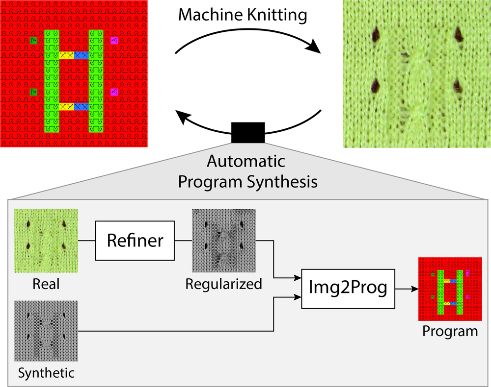
Figure 1: Illustration of our inverse problem and solution. An instruction map (top-left) is knitted into a physical artifact (top-right). We propose a machine learning pipeline to solve the inverse problem by leveraging synthetic renderings of the instruction maps.

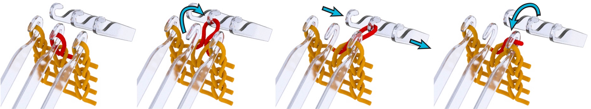
Figure 2: Sample Transfer sequence: move the red center stitch to the opposite bed; rack (move) the back bed 1 needle relative to the front; transfer the red stitch back to its original side. Note that the center front needle is now empty, while the right front needle holds 2 stitches.

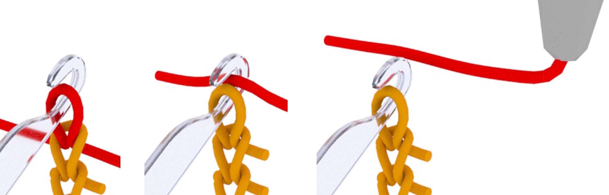
Figure 3: (L to R) Illustration of Knit, Tuck, and Miss operations.

The importance of patterning in textile design is evident in pattern books (Donohue, 2015; Shida & Roehm, 2017), which contain instructions for hundreds of decorative designs that have been manually crafted and tested over time. Unfortunately, these pattern libraries are geared towards hand-knitting and they are often incompatible with the operations of industrial knitting machines. Even in cases when a direct translation is possible, the patterns are only specified in stitch-level operation sequences. Hence, they would have to be manually specified and tested for each machine type similarly to low-level assembly programming.

In this work, we propose an inverse design method using deep learning to automate the pattern design for industrial knitting machines. In our inverse knitting, machine instructions are directly inferred from an image of the fabric pattern. To this end, we collect a paired dataset of knitting instruction maps and corresponding images of knitted patterns. We augment this dataset with synthetically generated pairs obtained using a knitting simulator (Shima Seiki, ). This combined dataset facilitates a learning-based approach. More specifically, we propose a theoretically inspired image-to-program map synthesis method that leverages both real and simulated data for learning. Our contributions include:

• An automatic translation of images to sequential instructions for a real manufacturing process;

• A diverse knitting pattern dataset that provides a mapping between images and instruction programs specified using a new domain-specific language (DSL) (Kant, 2018) that significantly simplifies low-level instructions and can be decoded without ambiguity;

• A theoretically inspired deep learning pipeline to tackle this inverse design problem; and

• A novel usage of synthetic data to learn to neutralize real-world, visual perturbations.

In the rest of the paper, we first provide the necessary background in machine knitting and explain our 2D regular instructions, we then go over our dataset acquisition, detail our learning pipeline making use of synthetic data, and finally go over our experiment results.

2 Knitting Background

Knitting is one of the most common forms of textile manufacturing. The type of knitting machine we are considering in this work is known as a V-bed machine, which allows automatic knitting of whole garments. This machine type uses two beds of individually controllable needles, both of which are oriented in an inverted V shape allowing opposite needles to transfer loops between beds. The basic operations are illustrated in Figures 2 and  3:

• Knit pulls a new loop of yarn through all current loops,

• Tuck stacks a new loop onto a needle,

• Miss skips a needle,

• Transfer moves a needle’s content to the other bed,

• Racking changes the offset between the two beds.

Whole garments (e.g. socks, sweatshirts, hats) can be automatically manufactured by scheduling complex sequences of these basic operations (Underwood, 2009; McCann et al., 2016). Furthermore, this manufacturing process also enables complex surface texture and various types of patterns. Our aim is to automatically generate machine instructions to reproduce any geometric pattern from a single close-up photograph (e.g. of your friend’s garment collection). To simplify the problem, we assume the input image only captures 2D patterning effects of flat fabric, and we disregard variations associated with the 3D shape of garments.

3 Instruction Set

K

P

T

M

FR1

FR2

FL1

FL2

BR1

BR2

BL1

BL2

XR+

XR-

XL+

XL-

S

Figure 4: Top: abstract illustration and color coding of our $17$ instructions. Bottom: instruction codes, which can be interpreted using the initial character of the following names: Knit and Purl (front and back knit stitches), Tuck, Miss, Front, Back, Right, Left, Stack. Finally, X stands for Cross where $+$ and $-$ are the ordering (upper and lower). Move instructions are composed of their initial knitting side (Front or Back), the move direction (Left or Right) and the offset (1 or 2).

General knitting programs are sequences of operations which may not necessarily have a regular structure. In order to make our inverse design process more tractable, we devise a set of $17$ pattern instructions (derived from a subset of the hundreds of instructions from (Shima Seiki, )). These instructions include all basic knitting pattern operations and they are specified on a regular 2D grid that can be parsed and executed line-by-line. We first detail these instructions and then explain how they are sequentially processed.

The first group of instructions are based on the first three operations, namely: Knit, Tuck and Miss.

Then, transfer operations allow moving loops of yarn across beds. This is important because knitting on the opposite side produces a very distinct stitch appearance known as reverse stitch or Purl – our complement instruction of Knit.

Furthermore, the combination of transfers with racking allows moving loops within a bed. We separate such higher-level operations into two groups: Move instructions only consider combinations that do not cross other such instructions so that their relative scheduling does not matter, and Cross instructions are done in pairs so that both sides are swapped, producing what is known as cable patterns. The scheduling of cross instructions is naturally defined by the instructions themselves. These combined operations do not create any new loop by themselves, and thus we assume they all apply a Knit operation before executing the associated needle moves, so as to maintain spatial regularity.

Finally, transfers also allow different stacking orders when multiple loops are joined together. We model this with our final Stack instruction. The corresponding symbols and color coding of the instructions are shown in Figure 4.

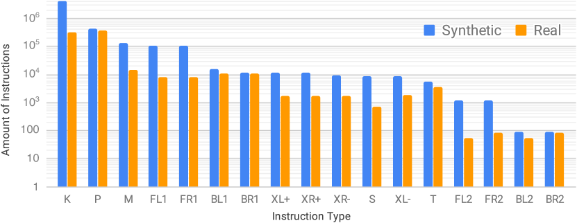
Figure 5: Instruction counts in descending order, for synthetic and real images. Note the logarithmic scale of the Y axis.

3.1 Knitting Operation Scheduling

Given a line of instructions, the sequence of operations is done over a full line using the following steps:

1. The current stitches are transferred to the new instruction side without racking;

2. The base operation (knit, tuck or miss) is executed;

3. The needles of all transfer-related instructions are transferred to the opposite bed without racking;

4. Instructions that involve moving within a bed proceed to transfer back to the initial side using the appropriate racking and order;

5. Stack instructions transfer back to the initial side without racking.

Instruction Side

The only instructions requiring an associated bed side are those performing a knit operation. We thus encode the bed side in the instructions (knit, purl, moves), except for those where the side can be inferred from the local context. This inference applies to Cross which use the same side as past instructions (for aesthetic reasons), and Stack which uses the side of its associated Move instruction. Although this is a simplification of the design space, we did not have any pattern with a different behaviour.

4 Dataset for Knitting Patterns

Before developing a learning pipeline, we describe our dataset and its acquisition process. The frequency of different instruction types is shown in Figure 5.

The main challenge is that, while machine knitting can produce a large amount of pattern data reasonably quickly, we still need to specify these patterns (and thus generate reasonable pattern instructions), and acquire calibrated images for supervised learning.

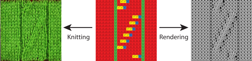
Figure 6: Different parts of our dataset (from left to right): real data images, machine instructions, and black-box rendering.

4.1 Pattern Instructions

We extracted pattern instructions from the proprietary software KnitPaint (Shima Seiki, ). These patterns have various sizes and span a large variety of designs from cable patterns to pointelle stitches, lace, and regular reverse stitches.

Given this set of initial patterns (around a thousand), we normalized the patterns by computing crops of $20\times 20$ instructions with $50\%$ overlap, while using default front stitches for the background of smaller patterns. This provided us with 12,392 individual $20\times 20$ patterns (after pruning invalid patterns since random cropping can destroy the structure).

We then generated the corresponding images in two different ways: (1) by knitting a subset of 1,044 patches, i.e., Real data, and (2) by rendering all of them using the basic pattern preview from KnitPaint, i.e., Simulated data. See Figure 6 for sample images.

4.2 Knitting Many Samples

The main consideration for capturing knitted patterns is that their tension should be as regular as possible so that knitting units would align with corresponding pattern instructions. We initially proceeded with knitting and capturing patterns individually but this proved to not be scalable.

We then chose to knit sets of $25$ patterns over a $5\times 5$ tile grid, each of which would be separated by both horizontal and vertical tubular knit structures. The tubular structures are designed to allow sliding $1/8$ inch steel rods which we use to normalize the tension, as shown in Figure 7. Note that each knitted pattern effectively provides us with two full opposite patterns (the front side, and its back whose instructions can be directly mapped from the front ones). This doubles the size of our real knitted dataset to 2,088 samples after annotating and cropping the knitted samples.

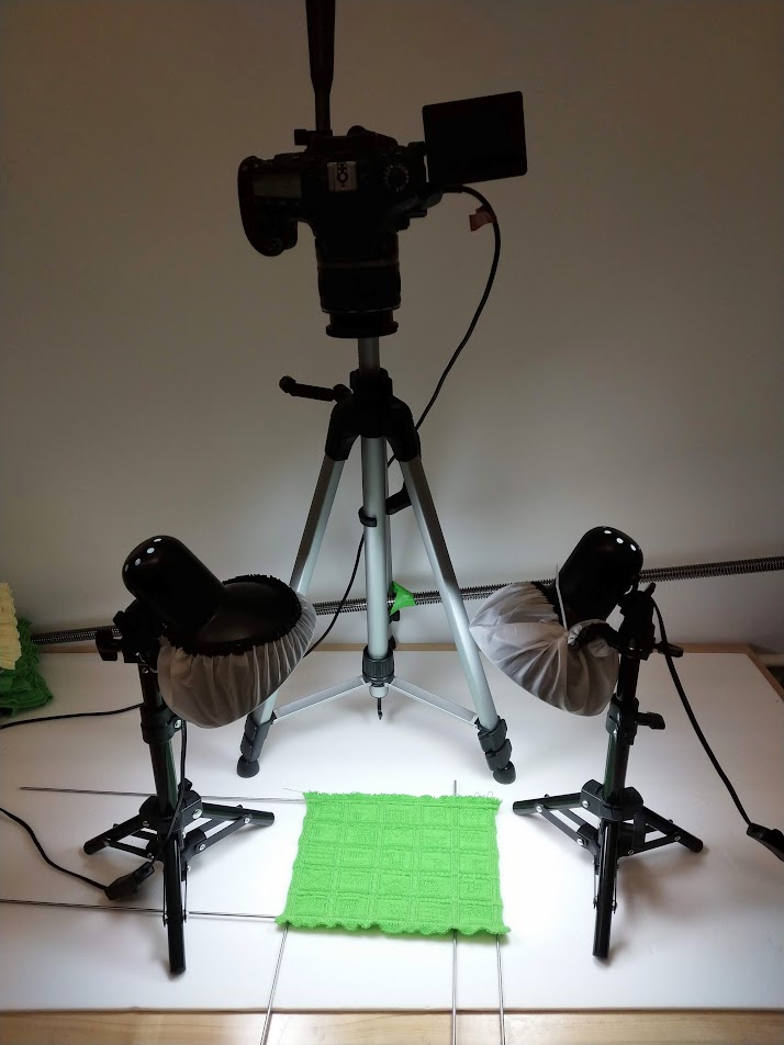
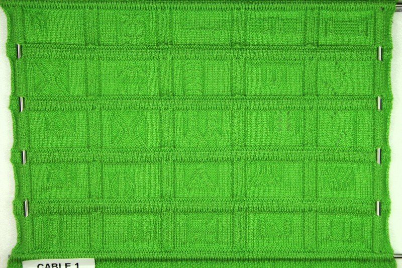
Figure 7: Our basic capture setup and a sample of $5\times 5$ knitted patterns with tension controlled by steel rods.

5 Instruction Synthesis Model

We present our deep neural network model that infers a 2D knitting instruction map from an image of patterns. In this section, we provide the theoretical motivation of our framework, and then we describe the loss functions we used, as well as implementation details.

5.1 Learning from different domains

When we have a limited number of real data, it is appealing to leverage simulated data because high quality annotations are automatically available. However, learning from synthetic data is problematic due to apparent domain gaps between synthetic and real data. We study how we can further leverage simulated data. We are motivated by the recent work, Simulated+Unsupervised (S+U) learning (Shrivastava et al., 2017), but in contrast to them, we develop our framework from the generalization error perspective.

Let ${\mathcal{X}}$ be input space (image), and ${\mathcal{Y}}$ output space (instruction label), and ${\mathcal{D}}$ a data distribution on ${\mathcal{X}}$ paired with a true labeling function $y_{\mathcal{D}}{:}\,{\mathcal{X}}{\rightarrow}{\mathcal{Y}}$. As a typical learning problem, we seek a hypothesis classifier $h{:}\,{\mathcal{X}}{\rightarrow}{\mathcal{Y}}$ that best fits the target function $y$ in terms of an expected loss: ${\mathcal{L}}_{\mathcal{D}}(h,h^{\prime}){=}\mathbb{E}_{x\sim{\mathcal{D}}}[l\left(h(x),h^{\prime}(x)\right)]$ for classifiers $h,h^{\prime}$, where $l{:}\,{\mathcal{Y}}{\times}{\mathcal{Y}}\,{\rightarrow}\,\mathbb{R}_{+}$ denotes a loss function. We denote its empirical loss as ${\hat{\mathcal{L}}_{\hat{\mathcal{D}}}}(h,h^{\prime})=\tfrac{1}{|{\hat{\mathcal{D}}}|}\sum_{i=1}^{|{\hat{\mathcal{D}}}|}l(h(x_{i}),h^{\prime}(x_{i}))$, where $\hat{\mathcal{D}}{=}\{x\}$ is the sampled dataset.

In our problem, since we have two types of data available, a source domain ${\mathcal{D}}_{S}$ and a target domain ${\mathcal{D}}_{T}$ (which is real or simulated as specified later), our goal is to find $h$ by minimizing the combination of empirical source and target losses as $\alpha$-mixed loss, ${\hat{\mathcal{L}}}_{\alpha}(h,y)=\alpha{\hat{\mathcal{L}}}_{S}(h,y)+(1{-}\alpha){\hat{\mathcal{L}}}_{T}(h,y),$ where $0{\leq}\alpha{\leq}1$, and for simplicity we shorten ${\mathcal{L}}_{{\mathcal{D}}_{\{S,T\}}}{=}{\mathcal{L}}_{\{S,T\}}$ and we use the parallel notation ${\mathcal{L}}_{\{S,T\}}$ and $\hat{{\mathcal{L}}}_{\{S,T\}}$. Our underlying goal is to achieve a minimal generalized target loss ${\mathcal{L}}_{T}$. To develop a generalizable framework, we present a bound over the target loss in terms of its empirical $\alpha$-mixed loss, which is a slight modification of Theorem 3 of (Ben-David et al., 2010).

Theorem 1.

Let ${\mathcal{H}}$ be a hypothesis class, and ${\mathcal{S}}$ be a labeled sample of size $m$ generated by drawing $\beta m$ samples from ${\mathcal{D}}_{S}$ and $(1-\beta)m$ samples from ${\mathcal{D}}_{T}$ and labeling them according to the true label $y$. Suppose ${\mathcal{L}}$ is symmetric and obeys the triangle inequality. Let $\hat{h}\in{\mathcal{H}}$ be the empirical minimizer of ${\hat{h}}=\operatornamewithlimits{\arg\min}_{h}{\hat{\mathcal{L}}}_{\alpha}(h,y)$ on ${\mathcal{S}}$ for a fixed $\alpha\in[0,1]$, and $h^{*}_{T}=\operatornamewithlimits{\arg\min}_{h}{\mathcal{L}}_{T}(h,y)$ the target error minimizer. Then, for any $\delta\in(0,1)$, with probability at least $1-\delta$ (over the choice of the samples), we have

$$\tfrac{1}{2}|{\mathcal{L}}_{T}({\hat{h}},y)-{{\mathcal{L}}}_{T}(h^{*}_{T},y)|\leq\alpha\left(\mathrm{disc}_{\mathcal{H}}({\mathcal{D}}_{S},{\mathcal{D}}_{T})+\lambda\right)+\epsilon,$$ (1)

where $\epsilon(m,\alpha,\beta,\delta)=\sqrt{\tfrac{1}{2m}\left(\tfrac{\alpha^{2}}{\beta}+\tfrac{(1-\alpha)^{2}}{1-\beta}\right)\log(\tfrac{2}{\delta})}$, and $\lambda{=}\min_{h\in{\mathcal{H}}}{\mathcal{L}}_{S}(h,y){+}{\mathcal{L}}_{T}(h,y)$.

The proof can be found in the supplementary material. Compared to (Ben-David et al., 2010), Theorem 1 is purposely extended to use a more general definition of discrepancy $\textrm{disc}_{{\mathcal{H}}}(\cdot,\cdot)$ (Mansour et al., 2009) that measures the discrepancy of two distributions (the definition can be found in the supplementary material) and to be agnostic to the model type (simplification), so that we can clearly present our motivation of our model design.

Theorem 1 shows that mixing two sources of data is possible to achieve a better generalization in the target domain. The bound is always at least as tight as either of $\alpha=0$ or $\alpha=1$ (The case that uses either source or target dataset alone). Also, as the total number of the combined data sample $m$ is larger, a tighter bound can be obtained. We consider 0-1 loss for $l$ in this section for simplicity, but not limited to.

A factor that the generalization gap (the right hand side in Eq. (1)) strongly depends on is the discrepancy $\mathrm{disc}_{\mathcal{H}}({\mathcal{D}}_{S},{\mathcal{D}}_{T})$. This suggests that we can achieve a tighter bound if we can reduce $\mathrm{disc}_{\mathcal{H}}({\mathcal{D}}_{S},{\mathcal{D}}_{T})$. We re-parameterize the target distribution ${\mathcal{D}}_{T}$ as ${\mathcal{D}}_{R}$ so that ${\mathcal{D}}_{T}{=}g\circ{\mathcal{D}}_{R}$, where $g$ is a distribution mapping function. Then, we find the mapping $g^{*}$ that leads to the minimal discrepancy for the empirical distribution ${\hat{\mathcal{D}}}_{R}$ as:

$$g^{*}= \operatornamewithlimits{\arg\min}\nolimits_{g}\mathrm{disc}_{\mathcal{H}}({\hat{\mathcal{D}}}_{S},~{}g\circ{\hat{\mathcal{D}}}_{R})$$

$$= \operatornamewithlimits{\arg\min}\nolimits_{g}\max_{h,h^{\prime}\in{\mathcal{H}}}|{\mathcal{L}}_{{\hat{\mathcal{D}}}_{S}}(h,h^{\prime})-{\mathcal{L}}_{g\circ{\hat{\mathcal{D}}}_{R}}(h,h^{\prime})|,$$ (2)

which is a min-max problem. Even though the problem is defined for an empirical distribution, it is intractable to search the entire solution space; thus, motivated by (Ganin et al., 2016), we approximately minimize the discrepancy by generative adversarial networks (GAN) (Goodfellow et al., 2014). Therefore, deriving from Theorem 1, our empirical minimization is formulated by minimizing the convex combination of source and target domain losses as well as the discrepancy as:

$${\hat{h},\hat{g}}=\operatornamewithlimits{\arg\min}_{h\in{\mathcal{H}},g\in{\mathcal{G}}}{\hat{\mathcal{L}}}_{\alpha}(h,y)+\tau\cdot\mathrm{disc}_{\mathcal{H}}({\hat{\mathcal{D}}}_{S},g{\circ}{\hat{\mathcal{D}}}_{R}).$$ (3)

Along with leveraging GAN, our key idea for reducing the discrepancy between two data distributions, i.e., domain gap, is to transfer the real knitting images (target domain, ${\hat{\mathcal{D}}}_{R}$) to synthetic looking data (source domain, ${\hat{\mathcal{D}}}_{S}$) rather than the other way around, i.e., making ${\hat{\mathcal{D}}}_{S}\approx\hat{g}\circ{\hat{\mathcal{D}}}_{R}$. The previous methods have investigated generating realistic looking images to adapt the domain gap. However, we observe that, when simulated data is mapped to real data, the mapping is a one-to-many mapping due to real-world effects, such as lighting variation, geometric deformation, background clutter, noise, etc. This introduces an unnecessary challenge to learn $g(\cdot)$; thus, we instead learn to neutralize the real-world perturbation by mapping from real data to synthetic looking data. Beyond simplifying the learning of $g(\cdot)$, it also allows the mapping to be utilized at test time for processing of real-world images.

We implement $h$ and $g$ using convolutional neural networks (CNN), and formulate the problem as a local instruction classification and represent the output as a 2D array of classification vectors $\mbox{ $\vec{\mathbf{s}}$}_{(i,j)}\in[0;1]^{K}$ (i.e., softmax values over $k\in K$) for our $K=17$ instructions at each spatial location $(i,j)$. In the following, we describe the loss we use to train our model $h\circ g$ and details about our end-to-end training procedure.

Loss function

We use the cross entropy for the loss ${\mathcal{L}}$. We supervise the inferred instruction to match the ground-truth instruction using the standard multi-class cross-entropy $\textrm{CE}(\mbox{ $\vec{\mathbf{s}}$},\mbox{ $\vec{\mathbf{y}}$})=-\sum_{k}y_{k}\log\left({s_{k}}\right)$ where $s_{k}$ is the predicted likelihood (softmax value) for instruction $k$, which we compute at each spatial location $(i,j)$.

For synthetic data, we have precise localization of the predicted instructions. In the case of the real knitted data, human annotations are imperfect and this can cause a minor spatial misalignment of the image with respect to the original instructions. For this reason, we allow the predicted instruction map to be globally shifted by up to one instruction. In practice, motivated by multiple instance learning (Dietterich et al., 1997), we consider the minimum of the per-image cross-entropy over all possibles one-pixel shifts (as well as the default no-shift variant), i.e., our complete cross entropy loss is

$$\mathcal{L}_{\textrm{CE}}=\frac{1}{Z_{CE}}\min_{d}\sum\nolimits_{i,j\in\mathcal{N}_{s}}\textrm{CE}(\mbox{ $\vec{\mathbf{s}}$}_{(i,j)+d},\mbox{ $\vec{\mathbf{y}}$}_{(i,j)}),$$ (4)

where $d\in\{(dx,dy)\,|\,dx,dy\in\{-1,0,+1\}\}$ is the pattern displacement for the real data and $d\in\{(0,0)\}$ for the synthetic data. The loss is accumulated over the spatial domain $\mathcal{N}_{s}=\{2,\dots,w{-}1\}{\times}\{2,\dots,h{-}1\}$ for the instruction map size $w\times h$ reduced by boundary pixels. $Z_{CE}=|\mathcal{N}_{s}|$ is a normalization factor.

5.2 Implementation details

Our base architecture is illustrated in Figure 1. We implemented it using TensorFlow (Abadi et al., 2016). The prediction network Img2prog takes $160{\times}160$ grayscale images as input and generates $20{\times}20$ instruction maps. The structure consists of an initial set of 3 convolution layers with stride 2 that downsample the image to $20{\times}20$ spatial resolution, a feature transformation part made of $6$ residual blocks (He et al., 2016; Zhu et al., 2017), and two final convolutions producing the instructions. The kernel size of all convolution layers is $3{\times}3$, except for the last layer which is $1{\times}1$. We use instance normalization (Ulyanov et al., 2016) for each of the initial down-convolutions, and ReLU everywhere.

We solve the minimax problem of the discrepancy $\textrm{disc}(\cdot,\cdot)$ w.r.t. $g$ using the least-square Patch-GAN (Zhu et al., 2017). Additionally, we add the perceptual loss and style loss (Johnson et al., 2016) between input real images and its generated images and between simulated images and generated images, respectively, to regularize the GAN training, which stably speeds up the training of $g$.

The structure of the Refiner network $g$ and the balance between losses can be found in the supplementary.

Training procedure

We train our network with a combination of the real knitted patterns and the rendered images. We have oversampled the real data to achieve 1:1 mix ratio with several data augmentation strategies, which can be found in the supplementary material. We train with 80% of the real data, withholding 5% for validation and 15% for testing, whereas we use all the synthetic data for training.

According to the typical training method for GAN (Goodfellow et al., 2014), we alternate the training between discriminator and the other networks, $h$ and $g$, but we update the discriminator only every other iteration, and the iteration is counted according to the number of updates for $h$ and $g$.

We trained our model for $150k$ iterations with batch size $2$ for each domain data using ADAM optimizer with initial learning rate $0.0005$, exponential decay rate $0.3$ every $50,000$ iterations. The training took from $3$ to ${4}$ hours (depending on the model) on a Titan Xp GPU.

6 Experiments

We first evaluate baseline models for our new task, along with an ablation study looking at the impact of our loss and the trade-off between real and synthetic data mixing. Finally, we look at the impact of the size of our dataset..

Accuracy Metric

For the same reason our loss in Eq. (4) takes into consideration a 1-pixel ambiguity along the spatial domain, we use a similarly defined accuracy. It is measured by the average of $\max_{d}\tfrac{1}{N_{\textrm{inst}}}\sum_{i,j}\mathbb{I}[{y_{\textrm{GT}}}_{(i,j)}\,{=}\,\operatornamewithlimits{\arg\max}_{k}{s}_{(i,j)+d}^{k}]$ over the whole dataset, where $N_{\textrm{inst}}=Z_{\textrm{CE}}$ is the same normalization constant as in Eq. (4), $y_{\textrm{GT}}$ the ground-truth label, $\mathbb{I}[\cdot]$ is the indicator function that returns 1 if the statement is true, 0 otherwise. We report two variants: FULL averages over all the instructions, whereas FG considers all instructions but the background (i.e., discard the most predominant instruction in the pattern).

Perceptual Metrics

For the baselines and the ablation experiments, we additionally provide perceptual metrics that measure how similar the knitted pattern would look. An indirect method for evaluation is to apply a pre-trained neural network to generated images and calculate statistics of its output, e.g., Inception Score (Salimans et al., 2016). Inspired by this, we learn a separate network to render simulated images of the generated instructions and compare it to the rendering of the ground truth using standard PSNR and SSIM metrics. Similarly to the accuracy, we allow for one instruction shift, which translates to full 8 pixels shifts in the image domain.

6.1 Comparison to Baselines

Table 1 compares the measured accuracy of predicted instructions on our real image test set. We also provide qualitative results in Figure 9.

Table 1: Performance comparison to baseline methods on our real image test dataset. The table shows translation invariant accuracy of the predicted instructions with and without the background and PSNR and SSIM metrics for the image reconstruction where available. More is better for all metrics used.

	Method	Accuracy (%)		Perceptual
		Full	FG	SSIM	PSNR [dB]
(a1)	CycleGAN (Zhu et al., 2017)	57.27	24.10	0.670	15.87
(a2)	Pix2Pix (Isola et al., 2017)	56.20	47.98	0.660	15.95
(a3)	UNet (Ronneberger et al., 2015)	89.65	63.99	0.847	21.21
(a4)	Scene Parsing (Zhou et al., 2018)	91.58	73.95	0.876	22.64
(a5)	S+U (Shrivastava et al., 2017)	91.32	71.00	0.864	21.42
(b1)	Img2prog (real only) with CE	91.57	71.37	0.866	21.62
(b2)	Img2prog (real only) with MILCE	91.74	72.30	0.871	21.58
(c1)	Refiner + Img2prog ($\alpha=0.9$)	93.48	78.53	0.894	23.28
(c2)	Refiner + Img2prog ($\alpha=2/3$)	93.58	78.57	0.892	23.27
(c3)	Refiner + Img2prog ($\alpha=0.5$)	93.57	78.30	0.895	23.24
(c4)	Refiner + Img2prog ($\alpha=1/3$)	93.19	77.80	0.888	22.72
(c5)	Refiner + Img2prog ($\alpha=0.1$)	92.42	74.15	0.881	22.27
(d1)	Refiner + Img2prog++ ($\alpha=0.5$)	94.01	80.30	0.899	23.56

The first 5 rows of Table 1-(a1-5) present results of previous works to provide snippets of other domain methods. For CycleGAN, no direct supervision is provided and the domains are mapped in a fully unsupervised manner. Together with Pix2pix, the two first methods do not use cross-entropy but L1 losses with GAN. Although they can provide interesting image translations, they are not specialized for multi-class classification problems, and thus cannot compete. All baselines are trained from scratch. Furthermore, since their architectures use the same spatial resolution for both input and output, we up-sampled instruction maps to the same image dimensions using nearest neighbor interpolation.

S+U Learning (Shrivastava et al., 2017) used a refinement network to generate a training dataset that makes existing synthetic data look realistic. In this case, our implementation uses our base network Img2prog and approximates real domain transfer by using style transfer. We tried two variants: using the original Neural Style Transfer (Gatys et al., 2016) and CycleGAN (Zhu et al., 2017). Both input data types lead to very similar accuracy (negligible difference) when added as a source of real data. We thus only report the numbers from the first one (Gatys et al., 2016).

Table 2: Performance of Refined+Img2prog++ measured per instruction over the test set. This shows that even though our instruction distribution has very large variations, our network is still capable of learning some representation for the least frequent instructions (3 orders of magnitude difference for FR2, FL2, BR2, BL2 compared to K and P).

Instruction	K	P	T	M	FR1	FR2	FL1	FL2	BR1	BR2	BL1	BL2	XR+	XR-	XL+	XL-	S
Accuracy [%]	96.52	96.64	74.63	66.65	77.16	100.00	74.20	83.33	68.73	27.27	69.94	22.73	60.15	62.33	60.81	62.11	25.85
Frequency [%]	44.39	47.72	0.41	1.49	1.16	0.01	1.23	0.01	1.22	0.02	1.40	0.02	0.22	0.18	0.19	0.22	0.12

6.2 Impact of Loss and Data Mixing Ratio

The second group in Table 1-(b1-2) considers our base network $h$ (Img2prog) without the refinement network $g$ (Refiner) that translates real images onto the synthetic domain. In this case, Img2prog maps real images directly onto the instruction domain. The results generated by all direct image translation networks trained with cross-entropy (a3-5) compare similarly with our base Img2prog on both accuracy and perceptual metrics. This shows our base network allows a fair comparison with the competing methods, and as will be shown, our final performance (c1-5, d1) is not gained from the design of Img2prog but Refiner.

The third group in Table 1-(c1-5) looks at the impact of the mixing ratio $\alpha$ when using our full architecture. In this case, the refinement network $g$ translates our real image into a synthetic looking one, which is then translated by Img2prog into instructions. This combination favorably improves both the accuracy and perceptual quality of the results with the best mixing ratio of $\alpha{=}2/3$ as well as a stable performance regime of $\alpha\in[0.5,0.9]$, which favors more the supervision from diverse simulated data. While $\epsilon$ in Theorem 1 has a minimum at $\alpha{=}\beta$, we have a biased $\alpha$ due to other effects, $\textrm{disc}(\cdot)$ and $\lambda$.

We tried learning the opposite mapping $g$ (from synthetic image to realistic looking), while directly feeding real data to $h$. This leads to detrimental results with mode collapsing. The learned $g$ maps to a trivial pattern and texture that injects the pattern information in invisible noise – i.e., adversarial perturbation – to enforce that $h$ maintains a plausible inference. We postulate this might be due to the non-trivial one-to-many mapping relationship from simulated data to real data, and overburden for $h$ to learn to compensate real perturbations by itself.

In the last row of Table 1-(d1), we present the result obtained with a variant network, Img2prog++ which additionally uses skip connections from each down-convolution of Img2prog to increase its representation power. This is our best model in the qualitative comparisons of Figure 9.

Finally, we check the per-instruction behavior of our best model, shown through the per-instruction accuracy in Table 2. Although there is a large difference in instruction frequency, our method still manages to learn some useful representation for rare instructions but the variability is high. This suggests the need for a systematic way of tackling the class imbalance (Huang et al., 2016; Lin et al., 2018).

6.3 Impact of Dataset Size

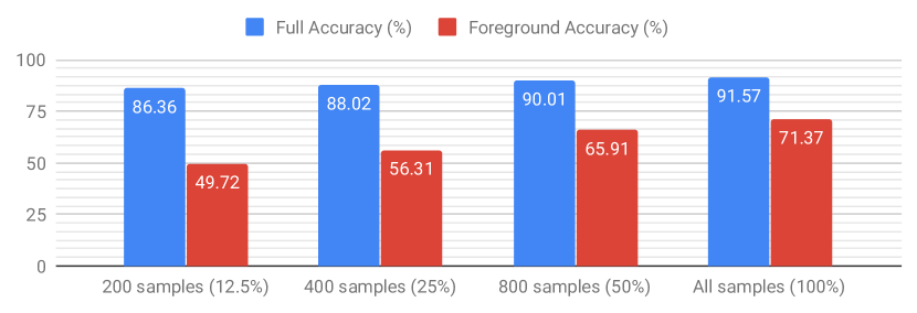
Figure 8: The impact of the amount of real training data (from 12.5% to 100% of the real dataset) over the accuracy.

In Figure 8, we show the impact of the real data amount on accuracy. As expected, increasing the amount of training data helps (and we have yet to reach saturation). With low amounts of data (here $400$ samples or less), the training is not always stable – some data splits lead to overfitting.

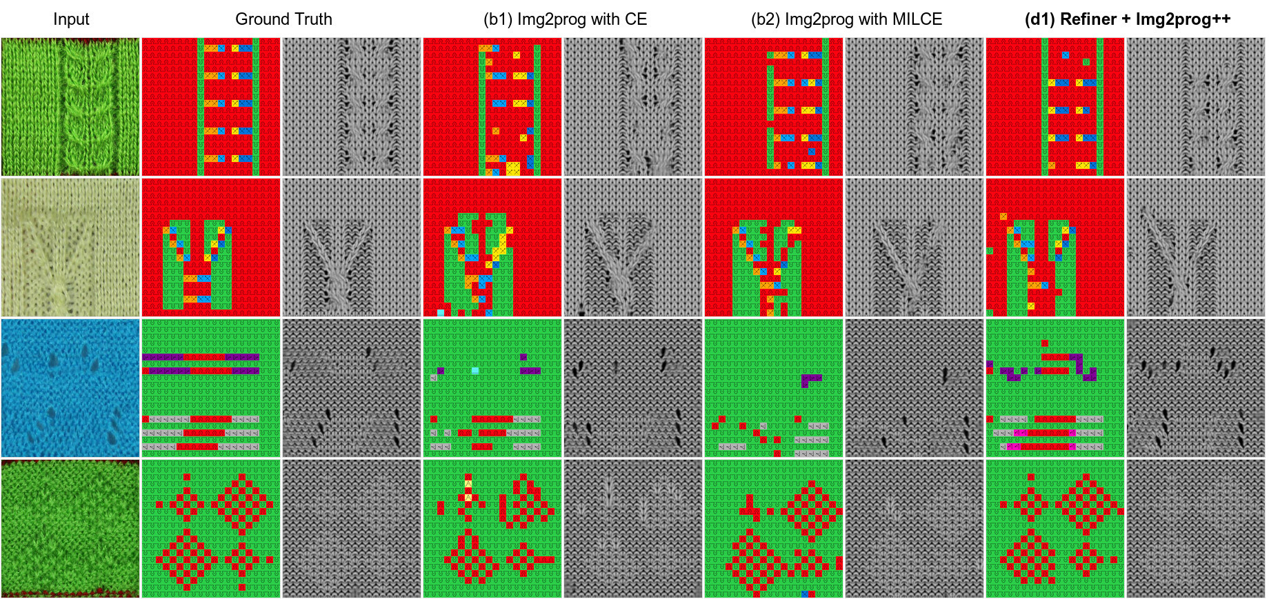
Figure 9: A comparison of instructions predicted by different versions of our method. We present the predicted instructions as well as a corresponding image from our renderer.

7 Discussion and Related Work

Knitting instruction generation We introduce automatic program synthesis for machine kitting using deep images translation. Recent works allow automatic conversion of 3D meshes to machine instructions (Narayanan et al., 2018), or directly model garment patterns on specialized meshes (Yuksel et al., 2012; Wu et al., 2018a), which can then be translated into hand knitting instruction (Wu et al., 2018b). While this does enable a wide range of achievable patterns, the accompanying interface requires stitch-level specification. This can be tedious, requires prior knitting experience and the resulting knits are not machine-knittable. We bypass the complete need of modeling these patterns and allow direct synthesis from image exemplars that are simpler to acquire and also machine knittable.

Simulated data based learning We demonstrate a way to effectively leverage both simulated and real knitting data. There have been a recent surge of adversarial learning based domain adaptation methods (Shrivastava et al., 2017; Tzeng et al., 2017; Hoffman et al., 2018) in the simulation-based learning paradigm. They deploy GANs and refiners to refine the synthetic or simulated data to look real. We instead take the opposite direction to exploit the simple and regular domain properties of synthetic data. Also, while they require multi-step training, our networks are end-to-end trained from scratch and only need a one-sided mapping rather than a two-sided cyclic mapping (Hoffman et al., 2018).

Semantic segmentation Our problem is to transform photographs of knit structures into their corresponding instruction maps. This resembles semantic segmentation which is a per-pixel multi-class classification problem except that the spatial extent of individual instruction interactions is much larger when looked at from the original image domain. From a program synthesis perspective, we have access to a set of constraints on valid instruction interactions (e.g. Stack is always paired with a Move instruction reaching it). This conditional dependency is referred to as context in semantic segmentation, and there have been many efforts to explicitly tackle this by Conditional Random Field (CRF) (Zheng et al., 2015; Chen et al., 2018; Rother et al., 2004). They clean up spurious predictions of a weak classifier by favoring same-label assignments to neighboring pixels, e.g., Potts model. For our problem, we tried a first-order syntax compatibility loss, but there was no noticeable improvement. However we note that (Yu & Koltun, 2016) observed that a CNN with a large receptive field but without CRF can outperform or compare similarly to its counterpart with CRF for subsequent structured guidance (Zheng et al., 2015; Chen et al., 2018). While we did not consider any CRF post processing in this work, sophisticated modeling of the knittability would be worth exploring as a future direction.

Another apparent difference between knitting and semantic segmentation is that semantic segmentation is an easy – although tedious – task for humans, whereas parsing knitting instructions requires vast expertise or reverse engineering.

Finally, we tried to use a state-of-the-art scene parsing network with very large capacity and pretraining (Zhou et al., 2018) which led to similar results to our best performing setup, but with a significantly more complicated model and training time. See the supplementary for details.

Neural program synthesis In terms of returning explicit interpretable programs, our work is closely related to program synthesis, which is a challenging, ongoing problem. The recent advance of deep learning has made notable progress in this domain, e.g., (Johnson et al., 2017; Devlin et al., 2017). Our task would have potentials to extend the research boundary of this field, since it differs from any other prior task on program synthesis in that: 1) while program synthesis solutions adopt a sequence generation paradigm (Kant, 2018), our type of input-output pairs are 2D program maps, and 2) the domain specific language is newly developed and applicable to practical knitting.

Limitations This work has two main limitations: (1) it does not explicitly model the pattern scale; and (2) it does not impose hard constraints on the output semantics, thus the intent of some instructions may be violated. We provide preliminary scale identification results in the supplementary, together with the details on the necessary post-processing that enables machine knitting of any output.

8 Conclusion

We have proposed an inverse process for translating high level specifications to manufacturing instructions based on deep learning. In particular, we have developed a framework that translates images of knitted patterns to instructions for industrial whole-garment knitting machines. In order to realize this framework, we have collected a dataset of machine instructions and corresponding images of knitted patterns. We have shown both theoretically and empirically how we can improve the quality of our translation process by combining synthetic and real image data. We have shown an uncommon usage of synthetic data to develop a model that maps real images onto a more regular domain from which machine instructions can more easily be inferred.

The different trends between our perceptual and semantic metrics bring the question of whether adding a perceptual loss on the instructions might also help improve the semantic accuracy. This could be done with a differentiable rendering system. Another interesting question is whether using higher-accuracy simulations (Yuksel et al., 2012; Wu et al., 2018a) could help and how the difference in regularity affects the generalization capabilities of our prediction.

We believe that our work will stimulate research to develop machine learning methods for design and manufacturing.

– Supplementary Material –
Neural Inverse Knitting: From Images to Manufacturing Instructions

Contents

• Details of the Refiner network.

• Loss balancing parameters.

• Used data augmentation details.

• Pattern scale identification.

• Post-processing details.

• Additional quantitative results.

• Additional qualitative results.

• Lemmas and theorem with the proofs.

Additional Resources

Additional knitting-related resources (the dataset, code and overview videos of the machine knitting process) can be found on our project page:
http://deepknitting.csail.mit.edu/

The Refiner Network

Our refinement network translates real images into regular images that look similar to synthetic images. Its implementation is similar to Img2prog, except that it outputs the same resolution image as input, of which illustration is shown in Figure 10.

Loss Balancing Parameters

When learning our full architecture with both Refiner and Img2prog, we have three different losses: the cross-entropy loss $\mathcal{L}_{CE}$, the perceptual loss $\mathcal{L}_{\textrm{Perc}}$, and the PatchGAN loss.

Our combined loss is the weighted sum

$$\mathcal{L}=\lambda_{\textrm{CE}}\mathcal{L}_{\textrm{CE}}+\lambda_{\textrm{Perc}}\mathcal{L}_{\textrm{Perc}}+\lambda_{\textrm{GAN}}\mathcal{L}_{\textrm{GAN}}$$ (5)

where we used the weights: $\lambda_{\textrm{CE}}=3$, $\lambda_{\textrm{Perc}}=0.02/(128)^{2}$ and $\lambda_{\textrm{GAN}}=0.2$. The losses $\mathcal{L}_{\textrm{Perc}}$ and $\lambda_{\textrm{GAN}}$ are measured on the output of Refiner, while the loss $\lambda_{\textrm{CE}}$ is measured on Img2prog.

The perceptual loss (Johnson et al., 2016) consists of the feature matching loss and style loss (using the gram matrix). If not mentioned here, we follow the implementation details of (Johnson et al., 2016), where VGG-16 (Simonyan & Zisserman, 2014) is used for feature extraction, after replacing max-pooling operations with average-pooling. The feature matching part is done using the pool3 layer, comparing the input real image and the output of Refiner so as to preserve the content of the input data. For the style matching part, we use the gram matrices of the {conv1_2, conv2_2, conv3_3} layers with the respective relative weights {0.3, 0.5, 1.0}. The measured style loss is between the synthetic image and the output of Refiner.

For ${\mathcal{L}}_{\textrm{GAN}}$ and the loss for the discriminator, the least-square Patch-GAN loss (Zhu et al., 2017) is used. We used $\{-1,1\}$ for the regression labels for respective fake and real samples insted of the label $\{0,1\}$ used in (Zhu et al., 2017).

For training, we normalize the loss $\lambda_{\textrm{CE}}$ to be balanced according to the data ratio of a batch. Specifically, for example, suppose a batch consisting of 2 real and 4 synthetic samples, respectively. Then, we inversely weighted the respective cross entropy losses for real and synthetic data by the weights of $\tfrac{4}{6}$ and $\tfrac{2}{6}$, so that the effects from the losses are balanced. This encourages the best performance to be expected at near $\alpha=0.5$ within a batch.

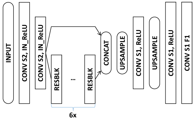
Figure 10: The illustration of the Refiner network architecture, where S$\#N$ denotes the stride size of $\#N$, IN_ReLU indicates the Instance normalization followed by ReLU, Resblk is the residual block that consists of ConvS1-ReLU-ConvS1 with shortcut connection (He et al., 2016), Upsample is the nearest neighbor upsampling with the factor $2\times$, $F$ is the output channel dimension. If not mentioned, the default parameters for all the convolutions are the stride size of 2, $F=64$, and the $3\times 3$ kernel size.

160

200

320

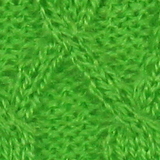
400

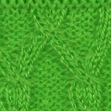
500

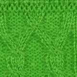
600

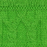
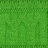
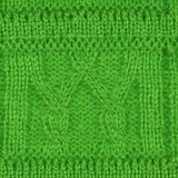
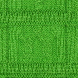
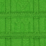
  700 800 900 1000 1500 2000

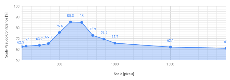
Figure 11: Scale identification experiment. Top row: cropped input image at corresponding scales with the correct pixel scale in bold with a light-gray background. Plot: pseudo-confidence curve showing a peak at the correct pixel scale ($600$).

Data Augmentation

We use multiple types of data augmentation to notably increase the diversity of yarn colors, lighting conditions, yarn tension, and scale:

• Global Crop Perturbation: we add random noise to the location of the crop borders for the real data images, and crop on-the-fly during training; the noise intensity is chosen such that each border can shift at most by half of one stitch;

• Local Warping: we randomly warp the input images locally using non-linear warping with linear RBF kernels on a sparse grid. We use one kernel per instruction and the shift noise is a 0-centered gaussian with $\sigma$ being $1/5$ of the default instruction extent in image space (i.e. $\sigma=8/5$);

• Intensity augmentation: we randomly pick a single color channel and use it as a mono-channel input, so that it provides diverse spectral characteristics. Also note that, in order to enhance the intensity scale invariance, we apply instance normalization (Ulyanov et al., 2016) for the upfront convolution layers of our encoder network.

Pattern scale identification

Our base system assumes that the input image is taken at a specific zoom level designed for our dataset, which is likely not going to be true for a random image. We currently assume this to be solved by the user given proper visual feedback (i.e., the user would see the pattern in real-time as they scan their pattern of interest with a mobile phone).

Here, we investigate the potential of automatically discovering the scale of the pattern. Our base idea is to evaluate the confidence of the output instruction map for different candidate scales and to choose the one with highest confidence. Although the softmax output cannot directly be considered as a valid probability distribution, it can serve as an approximation, which can be calibrated for (Guo et al., 2017). As a proof of concept, we take a full $5\times 5$ pattern image from our dataset and crop its center at different scales from $160$ pixels to $2000$ pixels of width. We then measure the output of the network and compute a scale pseudo-confidence as the average over pixels of the maximum softmax component.

In Figure 11, we show a sample image with crops at various scales, together with the corresponding uncalibrated pseudo-confidence measure, which peaks at around $600$ pixels scale. Coincidentally, this corresponds to the scale of our ground truth crops for that image.

This suggests two potential scenarios: (1) the user takes a much larger image and then that pattern image gets analysed offline to figure out the correct scale to work at using a similar procedure, and then generates a full output by using a tiling of crops at the detected scale, or (2) an interactive system could provide scale information and suggest the user to get closer to (or farther from) the target depending on the confidence gradient.

Table 3: Performance comparison with larger scene parsing network from (Zhou et al., 2018). (d2) uses pre-training on ImageNet (Russakovsky et al., 2015) and a much larger number of parameters (1.4M v.s. 51.4M).

	Method	Accuracy (%)		Perceptual		# Parameters
		Full	FG	SSIM	PSNR [dB]	(in Millions)
(d1)	Refiner + img2prog++ ($\alpha=1/2$)	94.01	80.30	0.899	23.56	1.4
(d2)	Large Scene Parsing w/ pre-training	94.95	83.46	0.908	24.58	51.4

Data post-processing

As mentioned in the main paper, our framework does not enforce hard constraint on the output semantics. This implies that some outputs may not be machine-knittable as-is.

More precisely, the output of our network may contain invalid instructions pairs or a lack thereof. We remedy to these conflicts by relaxing the conflicting instruction, which happens in only two cases:

1. Unpaired Cross instructions – we reduce such instructions into their corresponding Move variants (since Cross are Moves with relative scheduling), and

2. Cross pairs with conflicting schedules (e.g., both pair sides have same priority, or instructions within a pair’s side having different priorities) – in this case, we randomly pick a valid schedule (i.e., its impact is local).

This is sufficient to allow knitting on the machine. Note that Stack are semantically supposed to appear with a Move, but they don’t prevent knitting since their operations lead to the same as Knit when unpaired, and thus do not require any specific post-processing.

Additional quantitative results

The focus of the experiments in the main paper was on assessing specific trends such as the impact of the dataset size, or the different behaviours of baseline networks, the impact of mixing data types and the ratios of these.

As can be noted, we used a standard (residual) architecture and tried to avoid over-engineering our network or its parameters. However, we provide here results that show that we can obviously still do better by using more complex and larger networks, to the detriment of having to train for a longer time and resulting in a much larger model size.

In our baseline, we compared with a sample architecture from (Zhou et al., 2018), which we made small enough to compare with our baseline Img2prog implementation. Furthermore, our baseline implementations were all trained from scratch and did not make use of pre-training on any other dataset.

Here, we provide results for a much larger variant of that network, which we name Large Scene Parsing, and makes use of pre-training on ImageNet (Russakovsky et al., 2015). The quantitative comparison is provided in Table 3, which shows that we can achieve even better accuracy than our best current results using our Refiner+Img2prog++ combination. However, note that this comes with a much larger model size: ours has $1.4M$ parameters, whereas Large Scene Parsing has $51.4M$. Furthermore, this requires pre-training on ImageNet with millions of images (compared to our model working with a few thousands only).

Additional qualitative results

We present additional qualitative results obtained from several networks in Figure 12.

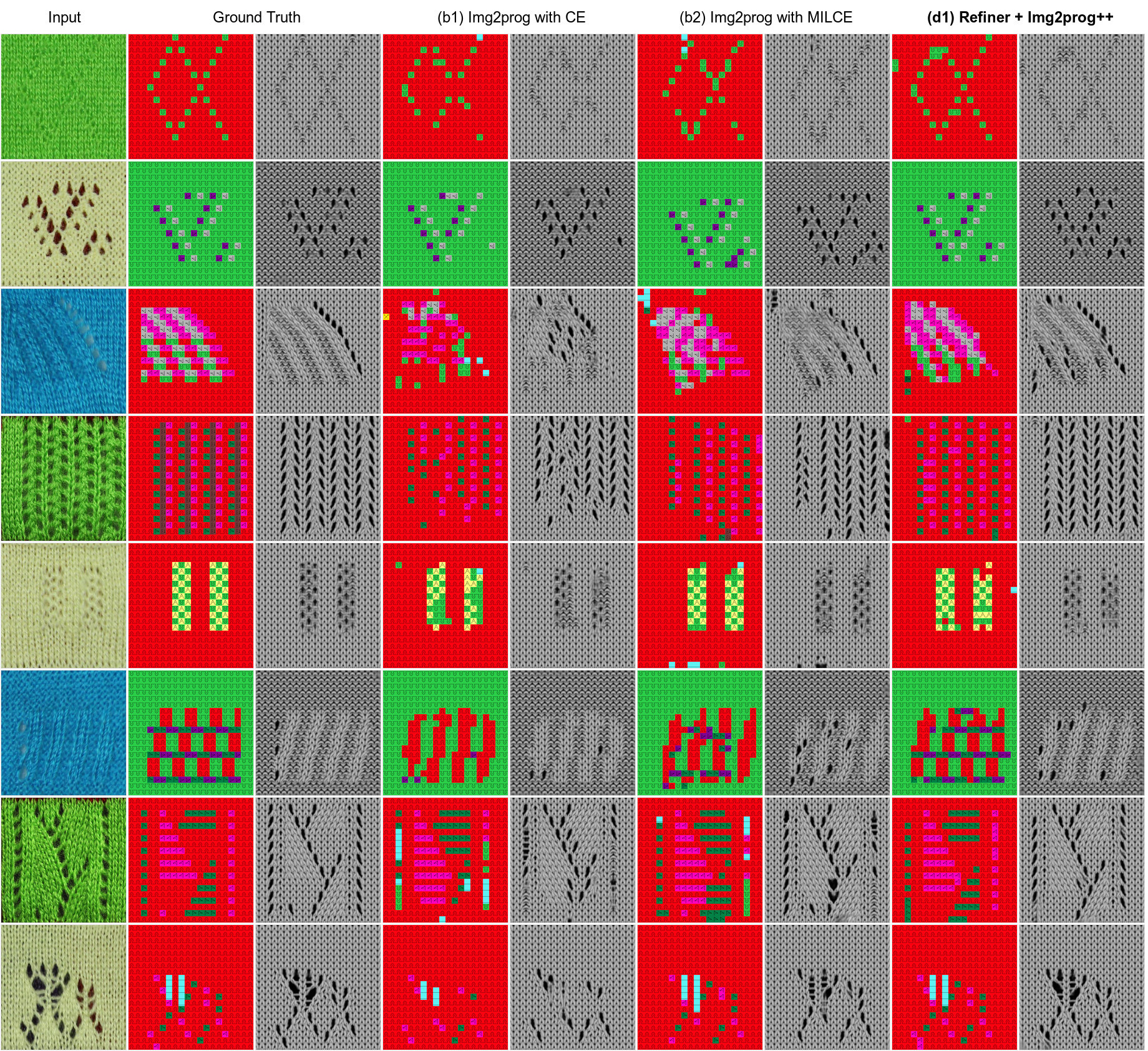
Figure 12: Additional comparisons of instructions predicted by different version of our method. We present the predicted instructions as well as a corresponding image from our renderer.

Proof of Theorem 1

We first describe the necessary definitions and lemmas to prove Theorem 1. We need a general way to measure the discrepancy between two distributions, which we borrow from the definition of discrepancy suggested by (Mansour et al., 2009).

Definition 1 (Discrepancy (Mansour et al., 2009)).

Let ${\mathcal{H}}$ be a class of functions mapping from ${\mathcal{X}}$ to ${\mathcal{Y}}$. The discrepancy between two distribution ${\mathcal{D}}_{1}$ and ${\mathcal{D}}_{2}$ over ${\mathcal{X}}$ is defined as

$$\mathrm{disc}_{\mathcal{H}}({\mathcal{D}}_{1},{\mathcal{D}}_{2})=\max\limits_{h,h^{\prime}{\in}{\mathcal{H}}}\left|{\mathcal{L}}_{{\mathcal{D}}_{1}}(h,h^{\prime})-{\mathcal{L}}_{{\mathcal{D}}_{2}}(h,h^{\prime})\right|.$$ (6)

The discrepancy is symmetric and satisfies the triangle inequality, regardless of any loss function. This can be used to compare distributions for general tasks even including regression.

The following lemma is the extension of Lemma 4 in (Ben-David et al., 2010) to be generalized by the above discrepancy.

Lemma 1.

Let $h$ be a hypothesis in class ${\mathcal{H}}$, and assume that ${\mathcal{L}}$ is symmetric and obeys the triangle inequality. Then

$$|{\mathcal{L}}_{\alpha}(h,y)-{\mathcal{L}}_{T}(h,y)|\leq\alpha\left(\mathrm{disc}_{\mathcal{H}}({\mathcal{D}}_{S},{\mathcal{D}}_{T})+\lambda\right),$$ (7)

where $\lambda{=}{\mathcal{L}}_{S}(h^{*},y){+}{\mathcal{L}}_{T}(h^{*},y)$, and the ideal joint hypothesis $h^{*}$ is defined as $h^{*}{=}\operatornamewithlimits{\arg\min}_{h\in{\mathcal{H}}}{\mathcal{L}}_{S}(h,y){+}{\mathcal{L}}_{T}(h,y)$.

Proof.

The proof is based on the triangle inequality of ${\mathcal{L}}$, and the last inequality follows the definition of the discrepancy.

$$|{\mathcal{L}}_{\alpha}(h,y)-{\mathcal{L}}_{T}(h,y)|$$

$$= \alpha|{\mathcal{L}}_{S}(h,y)-{\mathcal{L}}_{T}(h,y)|$$

$$= \alpha\left|{\mathcal{L}}_{S}(h,y)-{\mathcal{L}}_{S}(h^{*},h)+{\mathcal{L}}_{S}(h^{*},h)\right.$$

$$-{\mathcal{L}}_{T}(h^{*},h)+{\mathcal{L}}_{T}(h^{*},h)-{\mathcal{L}}_{T}(h,y)\left|\right.$$

$$\leq \alpha\big{|}\left|{\mathcal{L}}_{S}(h,y)-{\mathcal{L}}_{S}(h^{*},h)\right|+$$

$$\left|{\mathcal{L}}_{S}(h^{*},h)-{\mathcal{L}}_{T}(h^{*},h)\right|+\left|{\mathcal{L}}_{T}(h^{*},h)-{\mathcal{L}}_{T}(h,y)\right|\big{|}$$

$$\leq \alpha\big{|}{\mathcal{L}}_{S}(h^{*},y){+}|{\mathcal{L}}_{S}(h^{*},h){-}{\mathcal{L}}_{T}(h^{*},h)|{+}{\mathcal{L}}_{T}(h^{*},y)\big{|}$$

$$\leq \alpha\left(\mathrm{disc}_{\mathcal{H}}({\mathcal{D}}_{S},{\mathcal{D}}_{T})+\lambda\right).$$ (8)

We conclude the proof. ∎

Many types of losses satisfy the triangle inequality, e.g., the $0-1$ loss (Ben-David et al., 2010; Crammer et al., 2008) and $l_{1}$-norm obey the triangle inequality, and $l_{p}$-norm ($p>1$) obeys the pseudo triangle inequality (Galanti & Wolf, 2017).

Lemma 1 bounds the difference between the target loss and $\alpha$-mixed loss. In order to derive the relationship between a true expected loss and its empirical loss, we rely on the following lemma.

Lemma 2 ((Ben-David et al., 2010)).

For a fixed hypothesis $h$, if a random labeled sample of size $m$ is generated by drawing $\beta m$ points from ${\mathcal{D}}_{S}$ and $(1-\beta)m$ points from ${\mathcal{D}}_{T}$, and labeling them according to $y_{S}$ and $y_{T}$ respectively, then for any $\delta\in(0,1)$, with probability at least $1-\delta$ (over the choice of the samples),

$$|{\hat{\mathcal{L}}}_{\alpha}(h,y)-{{\mathcal{L}}}_{\alpha}(h,y)|\leq\epsilon(m,\alpha,\beta,\delta),$$ (9)

where $\epsilon(m,\alpha,\beta,\delta)=\sqrt{\tfrac{1}{2m}\left(\tfrac{\alpha^{2}}{\beta}+\tfrac{(1-\alpha)^{2}}{1-\beta}\right)\log(\tfrac{2}{\delta})}$.

The detail function form of $\epsilon$ will be omitted for simplicity. We can fix $m$, $\alpha$, $\beta$, and $\delta$ when the learning task is specified, then we can treat $\epsilon(\cdot)$ as a constant.

Theorem 1.

Let ${\mathcal{H}}$ be a hypothesis class, and ${\mathcal{S}}$ be a labeled sample of size $m$ generated by drawing $\beta m$ samples from ${\mathcal{D}}_{S}$ and $(1-\beta)m$ samples from ${\mathcal{D}}_{T}$ and labeling them according to the true label $y$. Suppose ${\mathcal{L}}$ is symmetric and obeys the triangle inequality. Let $\hat{h}\in{\mathcal{H}}$ be the empirical minimizer of ${\hat{h}}=\operatornamewithlimits{\arg\min}_{h}{\hat{\mathcal{L}}}_{\alpha}(h,y)$ on ${\mathcal{S}}$ for a fixed $\alpha\in[0,1]$, and $h^{*}_{T}=\operatornamewithlimits{\arg\min}_{h}{\mathcal{L}}_{T}(h,y)$ the target error minimizer. Then, for any $\delta\in(0,1)$, with probability at least $1-\delta$ (over the choice of the samples), we have

$$\tfrac{1}{2}|{\mathcal{L}}_{T}({\hat{h}},y)-{{\mathcal{L}}}_{T}(h^{*}_{T},y)|\leq\alpha\left(\mathrm{disc}_{\mathcal{H}}({\mathcal{D}}_{S},{\mathcal{D}}_{T})+\lambda\right)+\epsilon,$$ (10)

where $\epsilon(m,\alpha,\beta,\delta)=\sqrt{\tfrac{1}{2m}\left(\tfrac{\alpha^{2}}{\beta}+\tfrac{(1-\alpha)^{2}}{1-\beta}\right)\log(\tfrac{2}{\delta})}$, and $\lambda{=}\min_{h\in{\mathcal{H}}}{\mathcal{L}}_{S}(h,y){+}{\mathcal{L}}_{T}(h,y)$.

Proof.

We use Lemmas 1 and 2 for the bound derivation with their associated assumptions.

$${\mathcal{L}}_{T}({\hat{h}},y)$$

$$\leq{\mathcal{L}}_{\alpha}({\hat{h}},y)+\alpha\left(\mathrm{disc}_{\mathcal{H}}({\mathcal{D}}_{S},{\mathcal{D}}_{T})+\lambda\right),$$ (11)

(By Lemma 1)

$$\leq{\hat{\mathcal{L}}}_{\alpha}({\hat{h}},y)+\alpha\left(\mathrm{disc}_{\mathcal{H}}({\mathcal{D}}_{S},{\mathcal{D}}_{T})+\lambda\right)+\epsilon,$$ (12)

(By Lemma 2)

$$\leq{\hat{\mathcal{L}}}_{\alpha}(h^{*}_{T},y)+\alpha\left(\mathrm{disc}_{\mathcal{H}}({\mathcal{D}}_{S},{\mathcal{D}}_{T})+\lambda\right)+\epsilon,$$ (13)

$$\hskip 260.17464pt({\hat{h}}=\operatornamewithlimits{\arg\min}_{h\in{\mathcal{H}}}{\hat{\mathcal{L}}}_{\alpha}(h))$$

$$\leq{{\mathcal{L}}}_{\alpha}(h^{*}_{T},y)+\alpha\left(\mathrm{disc}_{\mathcal{H}}({\mathcal{D}}_{S},{\mathcal{D}}_{T})+\lambda\right)+2\epsilon,$$ (14)

(By Lemma 2)

$$\leq{{\mathcal{L}}}_{T}(h^{*}_{T},y)+2\alpha\left(\mathrm{disc}_{\mathcal{H}}({\mathcal{D}}_{S},{\mathcal{D}}_{T})+\lambda\right)+2\epsilon,$$ (15)

(By Lemma 1)

which concludes the proof. ∎

Theorem 1 does not have unnecessary dependencies for our purpose, which are used in (Ben-David et al., 2010) such as unsupervised data and the restriction of the model type to finite VC-dimensions.

References

- Abadi et al. (2016) Abadi et al. Tensorflow: a system for large-scale machine learning. In OSDI, 2016.
- Ben-David et al. (2010) Ben-David, S., Blitzer, J., Crammer, K., Kulesza, A., Pereira, F., and Vaughan, J. W. A theory of learning from different domains. Machine learning, 79(1-2):151–175, 2010.
- Chen et al. (2018) Chen, L.-C., Papandreou, G., Kokkinos, I., Murphy, K., and Yuille, A. L. Deeplab: Semantic image segmentation with deep convolutional nets, atrous convolution, and fully connected crfs. IEEE Transactions on Pattern Analysis and Machine Intelligence, 40(4):834–848, 2018.
- Crammer et al. (2008) Crammer, K., Kearns, M., and Wortman, J. Learning from multiple sources. Journal of Machine Learning Research, 9(Aug):1757–1774, 2008.
- Devlin et al. (2017) Devlin, J., Uesato, J., Bhupatiraju, S., Singh, R., Mohamed, A.-r., and Kohli, P. Robustfill: Neural program learning under noisy i/o. In International Conference on Machine Learning, 2017.
- Dietterich et al. (1997) Dietterich, T. G., Lathrop, R. H., and Lozano-Pérez, T. Solving the multiple instance problem with axis-parallel rectangles. Artificial intelligence, 89(1-2):31–71, 1997.
- Donohue (2015) Donohue, N. 750 Knitting Stitches: The Ultimate Knit Stitch Bible. St. Martin’s Griffin, 2015.
- Galanti & Wolf (2017) Galanti, T. and Wolf, L. A theory of output-side unsupervised domain adaptation. arXiv:1703.01606, 2017.
- Ganin et al. (2016) Ganin, Y., Ustinova, E., Ajakan, H., Germain, P., Larochelle, H., Laviolette, F., Marchand, M., and Lempitsky, V. Domain-adversarial training of neural networks. Journal of Machine Learning Research, 17(1):2096–2030, 2016.
- Gatys et al. (2016) Gatys, L. A., Ecker, A. S., and Bethge, M. Image style transfer using convolutional neural networks. In IEEE Conference on Computer Vision and Pattern Recognition, 2016.
- Goodfellow et al. (2014) Goodfellow, I., Pouget-Abadie, J., Mirza, M., Xu, B., Warde-Farley, D., Ozair, S., Courville, A., and Bengio, Y. Generative adversarial nets. In Advances in Neural Information Processing Systems, 2014.
- Guo et al. (2017) Guo, C., Pleiss, G., Sun, Y., and Weinberger, K. Q. On calibration of modern neural networks. In Proceedings of the 34th International Conference on Machine Learning-Volume 70, pp. 1321–1330. JMLR. org, 2017.
- He et al. (2016) He, K., Zhang, X., Ren, S., and Sun, J. Deep residual learning for image recognition. In IEEE Conference on Computer Vision and Pattern Recognition, 2016.
- Hoffman et al. (2018) Hoffman, J., Tzeng, E., Park, T., Zhu, J.-Y., Isola, P., Saenko, K., Efros, A. A., and Darrell, T. Cycada: Cycle-consistent adversarial domain adaptation. In International Conference on Machine Learning, 2018.
- Huang et al. (2016) Huang, C., Li, Y., Loy, C. C., and Tang, X. Learning deep representation for imbalanced classification. In IEEE Conference on Computer Vision and Pattern Recognition (CVPR), 2016.
- Isola et al. (2017) Isola, P., Zhu, J.-Y., Zhou, T., and Efros, A. A. Image-to-image translation with conditional adversarial networks. In IEEE Conference on Computer Vision and Pattern Recognition, 2017.
- Johnson et al. (2016) Johnson, J., Alahi, A., and Fei-Fei, L. Perceptual losses for real-time style transfer and super-resolution. In European Conference on Computer Vision, 2016.
- Johnson et al. (2017) Johnson, J., Hariharan, B., van der Maaten, L., Hoffman, J., Fei-Fei, L., Zitnick, C. L., and Girshick, R. Inferring and executing programs for visual reasoning. In IEEE International Conference on Computer Vision, 2017.
- Kant (2018) Kant, N. Recent advances in neural program synthesis. arXiv:1802.02353, 2018.
- Lin et al. (2018) Lin, J., Narayanan, V., and McCann, J. Efficient transfer planning for flat knitting. In Proceedings of the 2nd ACM Symposium on Computational Fabrication, pp. 1. ACM, 2018.
- Mansour et al. (2009) Mansour, Y., Mohri, M., and Rostamizadeh, A. Domain adaptation: Learning bounds and algorithms. In Conference on Learning Theory, 2009.
- McCann et al. (2016) McCann, J., Albaugh, L., Narayanan, V., Grow, A., Matusik, W., Mankoff, J., and Hodgins, J. A compiler for 3d machine knitting. ACM Transactions on Graphics, 35(4):49, 2016.
- Narayanan et al. (2018) Narayanan, V., Albaugh, L., Hodgins, J., Coros, S., and McCann, J. Automatic knitting of 3d meshes. ACM Transactions on Graphics, 2018.
- Ronneberger et al. (2015) Ronneberger, O., Fischer, P., and Brox, T. U-net: Convolutional networks for biomedical image segmentation. In International Conference on Medical image computing and computer-assisted intervention. Springer, 2015.
- Rother et al. (2004) Rother, C., Kolmogorov, V., and Blake, A. Grabcut: Interactive foreground extraction using iterated graph cuts. ACM Transactions on Graphics, 23(3):309–314, 2004.
- Russakovsky et al. (2015) Russakovsky, O., Deng, J., Su, H., Krause, J., Satheesh, S., Ma, S., Huang, Z., Karpathy, A., Khosla, A., Bernstein, M., et al. Imagenet large scale visual recognition challenge. International journal of computer vision, 115(3):211–252, 2015.
- Salimans et al. (2016) Salimans, T., Goodfellow, I., Zaremba, W., Cheung, V., Radford, A., and Chen, X. Improved techniques for training gans. In Advances in Neural Information Processing Systems, 2016.
- Shalev-Shwartz & Ben-David (2014) Shalev-Shwartz, S. and Ben-David, S. Understanding machine learning: From theory to algorithms. Cambridge university press, 2014.
- Shida & Roehm (2017) Shida, H. and Roehm, G. Japanese Knitting Stitch Bible: 260 Exquisite Patterns by Hitomi Shida. Tuttle Publishing, 2017.
- (30) Shima Seiki. SDS-ONE Apex3. http://www.shimaseiki.com/product/design/sdsone_apex /flat/. [Online; Accessed: 2018-09-01].
- Shrivastava et al. (2017) Shrivastava, A., Pfister, T., Tuzel, O., Susskind, J., Wang, W., and Webb, R. Learning from simulated and unsupervised images through adversarial training. In IEEE Conference on Computer Vision and Pattern Recognition, 2017.
- Simonyan & Zisserman (2014) Simonyan, K. and Zisserman, A. Very deep convolutional networks for large-scale image recognition. arXiv preprint arXiv:1409.1556, 2014.
- Tzeng et al. (2017) Tzeng, E., Hoffman, J., Saenko, K., and Darrell, T. Adversarial discriminative domain adaptation. In IEEE Conference on Computer Vision and Pattern Recognition, 2017.
- Ulyanov et al. (2016) Ulyanov, D., Vedaldi, A., and Lempitsky, V. Instance normalization: The missing ingredient for fast stylization. arXiv:1607.08022, 2016.
- Underwood (2009) Underwood, J. The design of 3d shape knitted preforms. Thesis, RMIT University, 2009.
- Wu et al. (2018a) Wu, K., Gao, X., Ferguson, Z., Panozzo, D., and Yuksel, C. Stitch meshing. ACM Transactions on Graphics (SIGGRAPH), 37(4):130:1–130:14, 2018a.
- Wu et al. (2018b) Wu, K., Swan, H., and Yuksel, C. Knittable stitch meshes. ACM Transactions on Graphics, 2018b.
- Yu & Koltun (2016) Yu, F. and Koltun, V. Multi-scale context aggregation by dilated convolutions. In International Conference on Learning Representations, 2016.
- Yuksel et al. (2012) Yuksel, C., Kaldor, J. M., James, D. L., and Marschner, S. Stitch meshes for modeling knitted clothing with yarn-level detail. ACM Transactions on Graphics (SIGGRAPH), 31(3):37:1–37:12, 2012.
- Zheng et al. (2015) Zheng, S., Jayasumana, S., Romera-Paredes, B., Vineet, V., Su, Z., Du, D., Huang, C., and Torr, P. H. Conditional random fields as recurrent neural networks. In IEEE International Conference on Computer Vision, 2015.
- Zhou et al. (2018) Zhou, B., Zhao, H., Puig, X., Xiao, T., Fidler, S., Barriuso, A., and Torralba, A. Semantic understanding of scenes through the ade20k dataset. International Journal of Computer Vision, 2018.
- Zhu et al. (2017) Zhu, J.-Y., Park, T., Isola, P., and Efros, A. A. Unpaired image-to-image translation using cycle-consistent adversarial networks. In IEEE International Conference on Computer Vision, 2017.