Decomposition of Plasma Kinetic Entropy into Position and Velocity Space and the Use of Kinetic Entropy in Particle-in-Cell Simulations

Abstract

We describe a systematic development of kinetic entropy as a diagnostic in fully kinetic particle-in-cell (PIC) simulations and use it to interpret plasma physics processes in heliospheric, planetary, and astrophysical systems. First, we calculate kinetic entropy in two forms – the “combinatorial” form related to the logarithm of the number of microstates per macrostate and the “continuous” form related to $f\ln f$, where $f$ is the particle distribution function. We discuss the advantages and disadvantages of each and discuss subtleties about implementing them in PIC codes. Using collisionless PIC simulations that are two-dimensional in position space and three-dimensional in velocity space, we verify the implementation of the kinetic entropy diagnostics and discuss how to optimize numerical parameters to ensure accurate results. We show the total kinetic entropy is conserved to three percent in an optimized simulation of anti-parallel magnetic reconnection. Kinetic entropy can be decomposed into a sum of a position space entropy and a velocity space entropy, and we use this to investigate the nature of kinetic entropy transport during collisionless reconnection. We find the velocity space entropy of both electrons and ions increases in time due to plasma heating during magnetic reconnection, while the position space entropy decreases due to plasma compression. This project uses collisionless simulations, so it cannot address physical dissipation mechanisms; nonetheless, the infrastructure developed here should be useful for studies of collisional or weakly collisional heliospheric, planetary, and astrophysical systems. Beyond reconnection, the diagnostic is expected to be applicable to plasma turbulence and collisionless shocks.

I Introduction

Dissipation of energy in nearly collisionless plasmas is a key component of understanding many fundamental plasma processes, such as magnetic reconnection, plasma turbulence, and collisionless shocks. In magnetic reconnection, dissipation can change magnetic topology (Hesse et al., 2011; Cassak, 2016) and may play a role in thermalizing plasma in the exhausts (Drake et al., 2006). In plasma turbulence, dissipation at kinetic scales is required to terminate the energy cascade (Cranmer, 2002; Parashar et al., 2009). A number of mechanisms for this conversion in weakly collisional plasmas have been discussed, including resonant and non-resonant wave-particle interactions and dissipation in coherent structures (i.e., intermittency) such as through reconnection (Howes, 2018). In collisionless shocks, dissipation is necessary to convert the upstream plasma bulk flow energy into thermal energy (Krall, 1997). These three fundamental processes underlie a staggering array of important applications in heliospheric, planetary, and astrophysical sciences, including supernova shocks (Reynolds, 2008), astrophysical jets (Beall, 2014), pulsar winds (Gaensler and Slane, 2006), interstellar shocks (Draine and McKee, 1993), shocks in galaxy cluster mergers (Enßlin et al., 1998), solar eruptions (Priest and Forbes, 2002), coronal heating (Klimchuk, 2006), solar wind turbulence (Gosling, 2007), solar wind-magnetosphere coupling and magnetospheric storms and substorms (Kivelson and Russell, 1995), and planetary shocks (Tsurutani and Stone, 2013).

The study of dissipation is at the forefront of research in these processes and settings, but it has been challenging to study it observationally, experimentally, numerically, and theoretically (Cassak, 2016; Howes, 2018). Recently, dissipation has become more accessible to study numerically through increases in computer power and observationally through the development of high cadence satellite measurements. For example, the primary objective of the Magnetospheric Multiscale (MMS) mission (Burch et al., 2016a) is dissipation accompanying reconnection (Burch et al., 2016b), and it has also been used to study magnetosheath turbulence (Servidio et al., 2017; Chen, Klein, and Howes, 2019) and the bow shock (Chen et al., 2018). Studying dissipation in solar wind turbulence would have been a key goal of the Turbulence Heating ObserveR (THOR) mission (Vaivads et al., 2016).

From a theoretical perspective, there have been efforts to identify regions where dissipation occurs. These measures have had some success in identifying the electron diffusion region (EDR) (Shay, Drake, and Swisdak, 2007) of magnetic reconnection (Zenitani et al., 2011; Swisdak, 2016; Burch et al., 2016b; Ashour-Abdalla et al., 2016) and dissipation in reconnection exhausts (Sitnov et al., 2018), and dissipation in plasma turbulence (Wan et al., 2016; Yang et al., 2017a, b). However, it is not clear which, if any, uniquely identifies genuine dissipation.

The present study is based on the premise that entropy is a natural candidate to identify and quantify dissipation. Entropy in a closed system is conserved in the absence of dissipation and monotonically increases when dissipation is present (Boltzmann, 1877; Bellan, 2008). Here, we interpret “dissipation” as a process that causes a total entropy increase in a closed, isolated system.

The fluid (thermodynamic) form of the entropy per particle for an isotropic plasma is related to $p/\rho^{\gamma}$, where $p$ is the (scalar) pressure, $\rho$ is the mass density, and $\gamma$ is the ratio of specific heats. This quantity has been studied in various settings for a long time. For example, stability of Earth’s magnetotail plasma sheet to the interchange instability is governed by fluid entropy (Erickson and Wolf, 1980; Borovsky et al., 1998; Kaufmann and Paterson, 2006; Wolf et al., 2006; Birn et al., 2009; Wolf et al., 2009; Johnson and Wing, 2009; Wang et al., 2009; Sanchez et al., 2012; Liu et al., 2014). Fluid entropy was specifically investigated in the context of magnetic reconnection, finding that it is conserved very well in magnetohydrodynamic (MHD) and particle-in-cell (PIC) simulations of reconnecting flux tubes (Birn et al., 2005; Birn, Hesse, and Schindler, 2006). Fluid entropy has been used to identify non-adiabatic heating during reconnection (Hesse et al., 2009; Ma and Otto, 2014). Lyubarsky and Kirk (2001) used fluid entropy in their study of reconnection in pulsar winds. Rowan, Sironi, and Narayan (2017) subtracted adiabatic heating from measured heating in the exhaust of a reconnection event in PIC simulations to find the leftover non-adiabatic contribution. A similar approach was used to study entropy production in collisionless shocks in PIC simulations (Guo, Sironi, and Narayan, 2017, 2018).

Many heliospheric, planetary, and astrophysical settings are only weakly collisional, so the fluid approximation may or may not be applicable. Instead, a kinetic approach is likely necessary in such settings, especially in regions with fine-scale spatial or temporal structures. We follow the convention by Kadanoff (2017) and refer to the version of entropy in kinetic theory as “kinetic entropy”. The theory will be reviewed in Appendix A.1.

Kinetic entropy has been a useful diagnostic in studies using the gyrokinetic model. In this model, the second order perturbed distribution function is related to the perturbed kinetic entropy (Krommes and Hu, 1994; Schekochihin et al., 2009) and the kinetic entropy production rate is related to the heating rate (Howes et al., 2006). Using gyrokinetic and related models, energy dissipation and plasma heating have been studied in simulations of magnetic reconnection (Loureiro, Schekochihin, and Zocco, 2013; Numata and Loureiro, 2015) and plasma turbulence (Watanabe and Sugama, 2004; Tatsuno et al., 2009; TenBarge and Howes, 2012; Nakata, Watanabe, and Sugama, 2012; TenBarge and Howes, 2013; Told et al., 2015; Li et al., 2016; Klein, Howes, and TenBarge, 2017; Grošelj et al., 2017). Kinetic entropy has also been investigated in studies of turbulence using the Vlasov-hybrid (Vlasov ions, fluid electrons) approach (Cerri, Kunz, and Califano, 2018) and in shocks (Margolin, 2017).

Meanwhile, the investigation of kinetic entropy in fully kinetic plasma systems, i.e., without any degrees of freedom integrated out, has been carried out in some observational and theoretical studies. Observational data was used to study kinetic entropy in Earth’s plasma sheet (Kaufmann and Paterson, 2009, 2011) and Earth’s bow shock (Parks et al., 2012). Dynamics of the magnetosphere was investigated using various entropy measures from statistics (Balasis et al., 2009). Generalizations of kinetic entropy to kappa-distributions in the solar wind have been studied (Leubner, 2004). The permutation entropy was used to analyze solar wind turbulence (Olivier, Engelbrecht, and Strauss, 2019). The entropy production in a kinetic-based fluid closure (Hammett and Perkins, 1990) was recently investigated (Sarazin et al., 2009). Kinetic mechanisms for the increase of entropy have been discussed for reconnection with an out-of-plane (guide) magnetic field (Hesse et al., 2017). A recent model of the turbulent cascade employs the kinetic entropy in a renormalization group approach (Eyink, 2018). However, we are not aware of any studies calculating kinetic entropy from first principles in fully kinetic PIC simulations.

There are challenges to use entropy as a diagnostic in a real system. First, the entropy can vary due to inhomogeneous plasma parameters, such as density and temperature, but mere convection should not be mistaken for dissipation. Moreover, equating an entropy increase with dissipation requires a closed system, but naturally occurring systems tend not to be closed. Despite these challenges the present approach is based on the view that studying entropy in fully kinetic models (from collisionless to collisional) in closed systems is useful to understand entropy production. The insights gained can be applied to understanding dissipation in real systems. Therefore, we argue that kinetic entropy can be a useful measure in collisionless systems, and can be crucial in collisional systems to identify dissipation. This is especially the case in the modern age of observational assets like MMS that measure particle distribution functions with a cadence of a fraction of a second and with high resolution in velocity space.

In this work, we describe a systematic development of kinetic entropy as a diagnostic in fully kinetic PIC simulations and investigate some of its uses to interpret plasma physics processes in heliospheric, planetary, and astrophysical systems. We implement two forms of kinetic entropy (Boltzmann, 1877; Planck, 1906) in our PIC code, the “combinatorial” and “continuous” forms. (Mouhot and Villani, 2011; Goldstein and Lebowitz, 2004) We use the kinetic entropy diagnostic on a two-dimensional in position space, three-dimensional in velocity space collisionless PIC simulation of antiparallel magnetic reconnection, though we expect it will be equally useful for simulations of plasma turbulence and collisionless shocks. Here, we summarize the new numerical and physical contributions resulting from this study:

1. We perform the first implementation (that we are aware) of the direct calculation of the combinatorial kinetic entropy in a PIC simulation, and provide a definitive assessment of its advantages and disadvantages relative to the more standard continuous kinetic entropy form.

2. We perform a careful validation of the kinetic entropy diagnostics as a function of numerical parameters, which is important to ensure proper application of this approach in future studies of reconnection or other applications. The discussion includes how to choose the velocity space grid scale and the number of macro-particles per grid cell $PPG$. We point out that macro-particles (also known as super-particles) in a PIC simulation represent a large number of actual particles in the system being simulated, and this needs to be properly accounted for to compare to observations or experiments.

3. We show the kinetic entropy increases by only 3% in a carefully constructed collisionless PIC simulation of magnetic reconnection. This gives the first estimate that we are aware of the fidelity one can expect from a collisionless PIC simulation in conserving kinetic entropy. The impact of this result on physics is that it shows it will be possible to include collisions into a PIC code and expect to be able to resolve its effect on the production of entropy through irreversible collisional processes. This is crucial for PIC studies of irreversible dissipation (which is a topic of future work).

4. We show that kinetic entropy is not reliably produced in simulations with a low number of particles per grid cell. We confirm simulations with a reduced number of particles can reproduce macroscopic quantities like the reconnection rate, but it may (depending on the PIC algorithm) give unphysical results for dissipation. This suggests caution is needed for low macro-particle per grid cell simulations on matters of kinetic entropy production, including particle acceleration and plasma heating. The present study provides a blueprint for how studies with a low number of particles per grid can determine if their numerics are impacting their physical results.

5. We decompose the total kinetic entropy into the sum of a position space and velocity space kinetic entropy. That this decomposition is possible seems to have been known previously in mathematical applications of plasma physics including Landau damping (Mouhot and Villani, 2011; Goldstein and Lebowitz, 2004), but to our knowledge this has not been exploited in applications to magnetized physical processes like magnetic reconnection (or turbulence or shocks). There are significant reasons this contribution is important to studies of entropy and dissipation. We show that this decomposition is helpful to understand the dynamics. For both electrons and ions, the position space entropy decreases in time during reconnection, while the velocity space entropy increases. This result has a clear physical interpretation, as the heating of particles leads to an increase in temperature and therefore an increase in velocity space entropy, while the compression of upstream particles into the current sheet and the magnetic islands leads to a decrease in position space entropy. Therefore, in collisionless systems in which total kinetic entropy is conserved, there is a conversion between the two types of kinetic entropy. This result is potentially important for observational studies of kinetic entropy. It reveals that an increase in the local velocity space kinetic entropy need not be associated with dissipation, as it also includes contributions from reversible energy conversion due to compression. Thus, caution must be employed when studying velocity space kinetic entropy.

   Another reason decomposing kinetic entropy into position and velocity space contributions is useful is that in nearly collisionless plasmas of heliophysical, astrophysical, and planetary interest, particle distributions can become strongly non-Maxwellian. The decomposition of a distribution into a thermal and non-thermal part is not possible for such complicated distributions. In a closed system that does not include collisions, the conservation of total kinetic entropy implies that any increase in velocity space entropy is balanced by an equal decrease to the position space entropy, and vice versa. In a closed collisional system, the two will not be balanced, and the net change of kinetic entropy gives a measure of the rate of dissipation. An example of a use of this is that one can tell by comparing the position and velocity space entropy what portion of the increase in velocity space kinetic entropy is reversible (the part that goes to position space kinetic entropy) and what portion is irreversible. This can be done from a calculation of the distribution function as a whole, without having to break it up into a thermal and non-thermal part, so it even works for distributions that are strongly non- Maxwellian.

It is worth noting that in the present study we develop a framework and perform a preliminary study, but we do not address the physical cause of dissipation because its presence in these simulations is purely numerical. One can show analytically that kinetic entropy increases only in the presence of collisions (Bellan, 2008). Since we use a collisionless PIC code for this study, the small kinetic entropy production we detect is due to numerical effects. We leave studies of mechanisms of dissipation for future work using a collisional PIC model.

This paper is organized as follows: in Sec. II, we briefly list the forms of kinetic entropy that we investigate. The existing theory of kinetic entropy including the fact that kinetic entropy can be decomposed into position and velocity space entropies is reviewed in Appendix A. Appendix B contains a thorough discussion of implementing the kinetic entropy diagnostic into PIC codes. Section III describes the setup of the simulations we employ. Section IV shows the simulation results, including a discussion of how to choose the diagnostic and simulation parameters to achieve robust results and a discussion of using kinetic entropy to obtain physical insights. Finally, conclusions, applications, and future work are discussed in Sec. V.

II Kinetic Entropies in This Study

In this section, we review the forms of kinetic entropy that we calculate in this study. The detailed derivation and discussion of the kinetic entropy expressions are given in Appendix A.

The “combinatorial Boltzmann entropy” $\mathcal{S}$ is defined in Eq. (13) as

$$\mathcal{S}=k_{B}\left[\ln N!-\sum_{j,k}\ln N_{jk}!\right],$$ (1)

where $N_{jk}$ is the number of particles in phase space bin spanning $(\vec{r}_{j},\vec{v}_{k})\rightarrow(\vec{r}_{j}+\Delta\vec{r},\vec{v}_{k}+\Delta\vec{v})$ and $N=\sum_{j,k}N_{jk}$ is the total number of particles. Since the total number of particles in a closed system is fixed, percentage changes in entropy are calculated based solely on the second term.

By using Stirling’s approximation and ignoring constant terms, one obtains the “continuous Boltzmann entropy” $S$ in Eq. (17) as

$$S=-k_{B}\int d^{3}{r}d^{3}vf(\vec{r},\vec{v})\left[\ln f(\vec{r},\vec{v})\right],$$ (2)

where $f(\vec{r},\vec{v})$ is the distribution function at position $\vec{r}$ and velocity $\vec{v}$ in phase space. The continuous Boltzmann entropy per unit volume, i.e., the continuous Boltzmann entropy density $s(\vec{r})$, is defined in Eq. (18) as

$$s(\vec{r})=-k_{B}\int d^{3}vf(\vec{r},\vec{v})\left[\ln f(\vec{r},\vec{v})\right].$$ (3)

The continuous Boltzmann entropy density $s_{M}(\vec{r})$ for a 3D drifting Maxwellian velocity distribution in local thermodynamic equilibrium (LTE) for a species of mass $m$, number density $n(\vec{r})$, bulk flow velocity $\vec{u}(\vec{r})$, and temperature $T(\vec{r})$, with $f(\vec{r},\vec{v})=f_{M}=n(\vec{r})[m/2\pi k_{B}T(\vec{r})]^{3/2}e^{-m[\vec{v}-\vec{u}(\vec{r})]^{2}/2k_{B}T(\vec{r})}$, follows directly. The result is in Eq. (19):

$$s_{M}(\vec{r})=\frac{3}{2}k_{B}n(\vec{r})\left[1+\ln\left(\frac{2\pi k_{B}T(\vec{r})}{mn^{2/3}(\vec{r})}\right)\right].$$ (4)

We use Eq. (4) to validate the implementation of the kinetic entropy diagnostic in our PIC code.

Both the combinatorial and continuous kinetic entropies can be decomposed into a sum of a position space entropy and a velocity space entropy. The derivation and discussion of the physical meaning of these two terms are reviewed in Appendix A.2. We define the combinatorial position space entropy $\mathcal{S}_{\text{position}}$ and velocity space entropy $\mathcal{S}_{\text{velocity}}$ in Eqs. (21) and (22) as

$$\mathcal{S}_{\text{position}}=k_{B}\left[\ln N!-\sum_{j}\ln N_{j}!\right],$$ (5)

$$\mathcal{S}_{\text{velocity}}=\sum_{j}k_{B}\left[\ln N_{j}!-\displaystyle\sum_{k}\ln N_{jk}!\right],$$ (6)

where $N_{j}$ is the total number of particles in the $j$th spatial bin by summing $N_{jk}$ only over velocity space. The continuous position space entropy $S_{\text{position}}$ and velocity space kinetic entropy $S_{\text{velocity}}$ are expressed in Eqs. (27)-(29) as

$$S_{\text{position}} = k_{B}\left[N\ln\left(\frac{N}{\Delta^{3}r}\right)\right.$$ (7)

$$- \left.\int d^{3}rn(\vec{r})\ln n(\vec{r})\right],$$

$$\textit{S}_{\text{velocity}} \int d^{3}rs_{\text{velocity}}(\vec{r}),$$ = (8)

$$s_{\text{velocity}}(\vec{r}) = k_{B}\left[n(\vec{r})\ln\left(\frac{n(\vec{r})}{\Delta^{3}v}\right)\right.$$ (9)

$$- \left.\int d^{3}vf(\vec{r},\vec{v})\ln f(\vec{r},\vec{v})\right],$$

where $\Delta^{3}r$ and $\Delta^{3}v$ are the volumes of the bins in position and velocity space, respectively , and $s_{\text{velocity}}(\vec{r})$ is the continuous velocity space kinetic entropy density whose spatial integral gives $S_{\text{velocity}}$. While it is possible in principle to define a continuous position space kinetic entropy density, it is not unique and it does not have a physical interpretation as the permutation of particles in position space, so we do not define a position space kinetic entropy density. Rather, we point out that the first term in Eq. (7) is a constant, so the time evolution of the position space kinetic entropy is solely determined by the spatial integral of $-n\ln n$.

Details about how to implement kinetic entropy diagnostics into a PIC code are discussed in Appendix B. The discussions include the importance of the actual number of particles per macro-particle, binning particles in phase space, obtaining the distribution function and kinetic entropies, and a comparison between combinatorial and continuous Boltzmann entropies.

III Simulations

Simulations are carried out using the p3d code (Zeiler et al., 2002), though we expect the diagnostic and analysis would be possible with any explicit PIC code. The code uses the relativistic Boris particle stepper (Birdsall and Langdon, 2004) for the particles and trapezoidal leapfrog (Guzdar et al., 1993) on the electromagnetic fields, with the fields allowed to have a smaller time step than the particles (half as big for our simulations). The divergence of the electric field is cleaned (every 10 particle time steps unless otherwise noted for our simulations) using the multigrid approach (Trottenberg, Oosterlee, and Schuller, 2000). Boundary conditions in every direction are periodic. The normalization is based on an arbitrary magnetic field strength $B_{0}$ and density $n_{0}$. Spatial and temporal scales are normalized to the ion inertial length $d_{i}=c/\omega_{pi}$ and the ion cyclotron time $\Omega_{ci}^{-1}$, respectively, where $\omega_{pi}=\sqrt{n_{0}e^{2}/\epsilon_{0}m_{i}}$ is the ion plasma frequency and $\Omega_{ci}=eB_{0}/m_{i}$ is the ion cyclotron frequency based on $n_{0}$ and $B_{0}$. Thus, velocities are normalized to the Alfvén velocity $v_{A}=d_{i}\Omega_{ci}$. Electric fields are normalized to $v_{A}B_{0}$. Pressures and temperatures are normalized to $B_{0}^{2}/\mu_{0}$ and $mv_{A}^{2}/k_{B}$, respectively. Entropies are normalized to Boltzmann’s constant $k_{B}$, though see Appendix B.4 for a discussion of the units of the continuous Boltzmann entropy.

For simplicity in this initial study, we only consider 2D in position space, 3D in velocity space simulations of symmetric anti-parallel magnetic reconnection. The simulation domain is $L_{x}\times L_{y}=51.2\times 25.6$. A double current sheet initial condition is used, with magnetic field given by $B_{x}(y)=\{\tanh[(y-3L_{y}/4)/w_{0}]-\tanh[(y-L_{y}/4)/w_{0}]+1\}$, where $w_{0}=0.5$ is the initial half-thickness of the current sheet. The initial velocity distribution functions are drifting Maxwellians with temperatures $T_{e}=1/12$ and $T_{i}=5/12$ for electrons and ions, respectively; both temperatures are initially uniform over the whole domain. We use these temperature values so that $v_{th,e}$ and $v_{th,i}$ are similar and a common velocity space bin size can be used (see Appendix B.2). The density is set to balance plasma pressure in the fluid sense, with $n(y)={\rm sech}^{2}[(y-L_{y}/4)/w_{0}]+{\rm sech}^{2}[(y-3L_{y}/4)/w_{0}]+n_{b}$, where $n_{b}=0.2$ is the background (lobe) density. Therefore, the total upstream plasma $\beta$ for this simulation is $n_{b}k_{B}(T_{e}+T_{i})/(B_{0}^{2}/2\mu_{0})=0.2$. Unlike the Geospace Environmental Modeling (GEM) magnetic reconnection challenge simulations (Birn et al., 2001), there is only one Maxwellian component in the current sheet. The ion-to-electron mass ratio $m_{i}/m_{e}=25$ and the speed of light $c$ is 15. These choices enforce that the plasma is non-relativistic (the speed of light exceeds the thermal and Alfvén speeds), which is appropriate for the non-relativistic treatment of kinetic entropy being considered here.

We use a small enough spatial grid scale and time step to ensure excellent conservation of energy and minimize numerical dissipation. We employ a time step of $\Delta t=0.001\ \Omega_{ci}^{-1}=0.025\ \Omega_{ce}^{-1}=0.075\ \omega_{pe}^{-1}$, which is a factor of about 2.67 smaller than what would typically be used for these simulation parameters. The smallest electron Debye length for this simulation (based on the maximum density of $1+n_{b}$) is $\lambda_{De}=0.018$. We select a grid scale of $\Delta x=\Delta y=0.0125\approx 0.6944\ \lambda_{De}$, again smaller than what is typically used for these simulation parameters to improve energy conservation.

Additional to the parameters for the PIC simulation, the kinetic entropy diagnostic requires a number of other parameters, which are discussed in detail in Appendix B. These parameters are only for the kinetic entropy diagnostic; they do not influence the rest of the simulation. As discussed in Appendix B.1, in order to calculate the combinatorial Boltzmann entropy $\mathcal{S}$ properly, the number of actual particles per macro-particle $a$ has to be specified at run time.

We first estimate $a$ using the method described in Appendix B.1. For the “base” simulation, the particle weight is proportional to the local density at $t=0$, with a value of $W=0.2/1.44$ in the lobe and $W=1.2/1.44$ at the center of current sheet. We use $PPG=100$ in the base simulation and, as calculated above, a grid scale of $\Delta x=0.6944\ \lambda_{De}$. To relate to the actual number of particles, we appeal to the system of interest being simulated. For a simulation representing the plasma in a solar active region, Table 1 gives $n\lambda_{De}^{3}\simeq 1.3\times 10^{7}$, so Eq. (30) gives $N_{cell}\simeq 4.3\times 10^{6}$ actual particles per grid cell. Using $W=0.2/1.44$, Eq. (32) gives $a=3.13\times 10^{5}$ actual particles per macro-particle. For the plasma sheet in Earth’s magnetotail, Table 1 gives $n\lambda_{De}^{3}\simeq 1.0\times 10^{13}$, so assuming the same weight and grid scale gives $a=2.5\times 10^{11}$. For what we refer to as the “base” simulation, we use $a=3.13\times 10^{5}$.

We also need to choose the velocity space bin size $\Delta v$ and the initial number of macro-particles per grid cell $PPG$ per species. For each, we must optimize these parameters, which is discussed in detail in Secs. IV.4 - IV.6. For the base simulation, we use $\Delta v=1$ and $PPG=100$. The velocity range for binning the particles is from $-12$ to $12$ in each dimension. Since the plasma is in the non-relativistic regime in this simulation, the choice of a broader velocity range than this should not make much difference.

IV Results

The layout of this section is as follows. We start with a validation of the implementation of the kinetic entropy diagnostics in the code in Sec. IV.1. The time evolution and conversion of energy and kinetic entropy is discussed in Sec. IV.2. We discuss the position and velocity space entropies in Sec. IV.3. Sections IV.4-IV.6 contain results on varying $a$, $PPG$, and $\Delta v$, respectively. Unless otherwise noted, the results presented here employ the implementation discussed in Appendix B on the base simulation described in Sec. III.

IV.1 Validation of the Kinetic Entropy Diagnostic

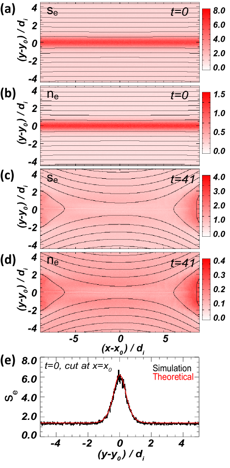
Figure 1: 2D plots, zoomed in near the reconnection X-line at $(x_{0},y_{0})$ of (a) electron kinetic entropy density $s_{e}$ and (b) electron density $n_{e}$ at time $t=0$. (c) and (d) are the same except at $t=41$. (e) A vertical cut of $s_{e}$ through the X-line (black) at $t=0$, with the theoretical prediction (red) overplotted.

Fig. 1(a) shows a 2D plot of the continuous Boltzmann entropy density $s_{e}(\vec{r})$ from Eq. (3) at time $t=0$ for electrons; results for ions are analogous. The center of the plot is shifted to the position of the X-line $(x_{0},y_{0})$ of the top current sheet at $y_{0}=3L_{y}/4$. Panel (b) shows the electron density $n_{e}$ at the same time. The structure of $s_{e}$ is strongly determined by the density, as expected from Eq. (4) for Maxwellian distributions such as those at the initial conditions of the present simulations. Panels (c) and (d) show similar plots, but for $t=41$, showing a similar relationship between kinetic entropy and density even though distribution functions are no longer all Maxwellian at this time.

The initial distribution functions for this simulation are drifting Maxwellians, so we can validate the implementation of the diagnostic by comparing the calculated $s_{e}$ with the analytic calculation in Eq. (4). In the upstream region where the density is 0.2, Eq. (4) predicts a value (in normalized code units) of $(3/2)(0.2)[1+\ln(2\pi(1/12)/(0.04\times 0.2^{2/3}))]=1.39$; in the center of the sheet where the density is 1.2 the analytic prediction is 6.21. Panel (e) shows a vertical cut of the continuous Boltzmann entropy density at $t=0$ in black, with the analytical prediction overplotted as the red line, revealing excellent agreement of the theory and simulations. In Sec. IV.4, we confirm that the combinatorial $\mathcal{S}$ and continuous $S$ Boltzmann entropies are in agreement, as they should be. We conclude that the kinetic entropy diagnostics implemented here successfully determine the kinetic entropy.

IV.2 Energy and Kinetic Entropy Conservation and Conversion

A principal diagnostic of momentum-conserving PIC codes is the conservation of total (particle plus electromagnetic) energy. Departures from perfect conservation occur only as a result of numerical effects including finite time step, finite grid scale, and noise introduced by having a finite number of macro-particles. In a collisionless PIC code, as is the case for the one employed in this study, kinetic entropy should also be conserved (Bellan, 2008), with departures from perfect conservation again only arising due to numerical effects. Here, we investigate energy and kinetic entropy conservation in our base simulation.

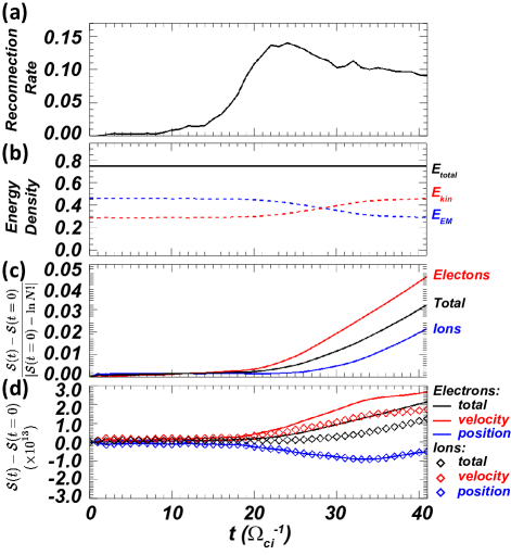
Figure 2: Time histories from the base simulation of the following quantities: (a) reconnection rate, (b) total energy density $E_{total}$ (black solid line), total kinetic energy density $E_{kin}$ (red dashed line), and electromagnetic energy density $E_{EM}$ (blue dashed line), (c) relative change of the non-constant term in the combinatorial Boltzmann entropy $\mathcal{S}(t)$ in Eq. (1) for electrons (red), ions (blue), and total (black), (d) deviation from its initial value of velocity space entropy $\mathcal{S}_{{\rm velocity}}$ (red), position space entropy $\mathcal{S}_{{\rm position}}$ (blue), and total combinatorial Boltzmann $\mathcal{S}$ (black) for electrons (solid curves) and ions (diamonds).

The time evolution of the system is shown using the reconnection rate as a function of time $t$ in Fig. 2(a). The reconnection rate is the time rate of change of magnetic flux between the X-line and O-line, identified at each time $t$ using the saddle and extremum of the magnetic flux function $\psi(\vec{r})$ defined by $\vec{B}=\hat{z}\times\nabla\psi$, where $\vec{B}$ is the magnetic field. As is typical in 2D PIC simulations in periodic domains, the reconnection rate starts to grow from zero (visibly at $t\approx 10$), reaches a peak (at $t\approx 21.5$), and then falls back down to a reasonably steady state (for $t>34$).

Fig. 2(b) shows total energy density $E_{total}$ (black solid curve), total kinetic energy density $E_{kin}$ (red dashed curve) including both bulk and thermal kinetic contributions, and total electromagnetic energy density $E_{EM}$ (blue dashed curve), as a function of time $t$ for the base simulation. The total energy only increases 0.24% by $t=41$; this is excellent total energy conservation. This is the result of our intentional use of a small time step and grid scale. The expected conversion of electromagnetic energy to kinetic energy during the reconnection process (starting in earnest at about $t=20$) is also seen in the time histories.

Now, we investigate how the kinetic entropy changes in time during the simulation, including both relative and absolute changes in kinetic entropy since both provide useful insights. For the relative change of the combinatorial Boltzmann entropy $\mathcal{S}$ in Eq. (1), it is important to note that $[\mathcal{S}(t)-\mathcal{S}(t=0)]/\mathcal{S}(t=0)$ is not a meaningful measure of the relative kinetic entropy change . This is because the combinatorial Boltzmann entropy $\mathcal{S}$ can be written as a sum of two terms [see Eq. (1)], and the first term is a large constant term. Thus, calculating the relative change in kinetic entropy merely as $[\mathcal{S}(t)-\mathcal{S}(t=0)]/\mathcal{S}(t=0)$ would be misleading, because each has a large term that does not change but skews the ratio. For this reason, we subtract out the constant term and report the change in kinetic entropy relative to the initial portion of the combinatorial kinetic entropy that can change, which is $\mathcal{S}(t=0)-k_{B}\ln N!$.

Fig. 2(c) shows the change of the combinatorial Boltzmann entropy in time from Eq. (1) normalized to $\mathcal{S}(t=0)-k_{B}\ln N!$ for the base simulation, with values for electrons in red, ions in blue, and their total in black. The relative changes are about 4.5%, 2.1% and 3.2% by $t$=41 for electrons, ions, and total, respectively. In general, the kinetic entropies are conserved reasonably well, given that reconnection occurs and there is a conversion of nearly one-third of the electromagnetic energy into particle kinetic energy. Interestingly, the kinetic entropy due to numerical effects is monotonically increasing. If the code had physical collisions, one would expect the kinetic entropy would monotonically increase. We find that the numerical effects, in this sense, mimic physical collisions.

The absolute change to the kinetic entropy is now used to study the partition between electrons and ions. Fig. 2(d) shows the total combinatorial Boltzmann entropy $\mathcal{S}$ (in black) for electrons (solid line) and ions (diamonds) as a function of time $t$. Each has its initial value subtracted so that the plotted values are the change relative to the initial time. Notice the change in the absolute kinetic entropies are quite large, at the $10^{13}$ level in code units (corresponding to the $10^{-10}$ level in units of J/K). This ostensibly large number is a result of the number of actual particles represented in the simulation being large. In particular, the base simulation has 100 $PPG$ and 4096 $\times$ 2048 cells, for a total of 838,860,800 macro-particles. With $a=3.13\times 10^{5}$, the total number of particles represented is $N=2.6\times 10^{14}$. The first term in the kinetic entropy in Eq. (14) is $\ln N!$, which is approximately $8.5\times 10^{15}$. This sets the scale of kinetic entropies for this system; we find the total kinetic entropies after the subtraction due to the second term in Eq. (14) are at the $10^{14}$ level, and the change in kinetic entropy in time is at the $10^{13}$ level, as seen in Fig. 2(d).

Comparing the total kinetic entropies for each individual species, we see that both increase in time as might be expected, but the electrons gain more than the ions in an absolute sense. This is very reasonable, as numerical effects arising at small scales are expected to disproportionately affect electrons.

IV.3 Position and Velocity Space Entropies

We now discuss the position and velocity space entropies discussed in Appendix A.2. The two terms are calculated from Eqs. (5) and (6) using the combinatorial Boltzmann entropy $\mathcal{S}$. Their evolution is shown in Fig. 2(d), with position space entropies in blue and velocity space entropies in red with electrons given by the solid lines and ions by the diamonds. First, we note that the position space entropy is essentially the same for electrons and ions. This is consistent with expectations as a result of quasi-neutrality of the plasma.

The velocity space entropy increases for both electrons and ions, a result of a temperature increase of both species due to the reconnection process, as expected from Appendix A.2. The increase in velocity space entropy is associated with a decrease in the position space entropy. If kinetic entropy is perfectly conserved, as the governing equations would have in this closed system, then any increase in velocity space entropy would necessarily be offset by a decrease in position space entropy. In the simulation, total kinetic entropy is not conserved perfectly, but we still observe a decrease in position space entropy for both electrons and ions. Physically, this decrease is associated with the enhanced density in the island as reconnection proceeds and upstream plasma is compressed. Compression leads to more particles in some phase space bins, lowering the position space entropy as discussed in Appendix A.2.

This explanation is predicated on the notion that the temperature increase is physical rather than numerical, so we investigate this here. The increase of total entropy due to numerical effects is less than 5%, as discussed in Sec. IV.2. One might expect the thermal energy change from numerical effects $\Delta E_{th,numerical}$ to scale like $Q_{numerical}\simeq T\Delta S_{numerical}$ from the first law of thermodynamics, so $\Delta E_{th,numerical}$ would be at the 5% level. However, in the simulation, the thermal energy gain for electrons and ions are 103% and 77%, respectively. This implies that physical heating is much more significant than the contribution due to numerical effects.

This result also underscores a point about temperature and entropy that is important to take into account in laboratory and satellite measurements of kinetic entropy. In this simulation, there is a significant increase in thermal energy, but only a small change in kinetic entropy. This shows that a temperature increase is not necessarily associated with an increase in total kinetic entropy.

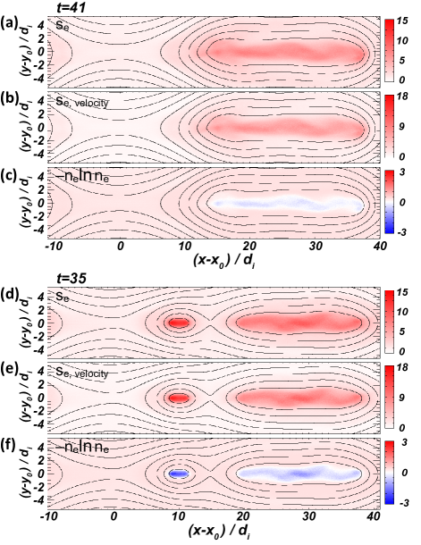
Figure 3: 2D plots of various electron kinetic entropies: (a) continuous Boltzmann entropy density $s_{e}(\vec{r})$, (b) velocity space entropy density $s_{e,{\rm velocity}}(\vec{r})$, (c) the $-n_{e}(\vec{r})\ln n_{e}(\vec{r})$ term that arises in the calculation of $S_{\text{position}}$, all evaluated at $t=41$. (d) - (f) are analogous plots at $t=35$, near the minimum in total position space kinetic entropy when there is a secondary island further compressing the plasma.

To get a sense for what the different kinetic entropies look like as a function of space, Fig. 3 includes plots of (a) continuous Boltzmann entropy density $s_{e}(\vec{r})$ [from Eq. (3)], (b) velocity space entropy density $s_{e,{\rm velocity}}(\vec{r})$ [from Eq. (9)], and (c) the $-n_{e}(\vec{r})\ln n_{e}(\vec{r})$ density related to the position space entropy [from Eq. (7)], each evaluated at $t=41$. These plots are all for electrons and are showing the whole domain in $x$ and are zoomed in to the upper current sheet in $y$.

Caution is needed in interpreting these plots. The regions of highest entropy in panels (a) and (b) do not necessarily reflect regions of increased kinetic entropy because the kinetic entropy at $t=0$ is not uniform in space since the plasma density is higher close to the center of the initial current sheet, as is shown near the current sheet in Fig. 1(a). Similarly, assessing the temporal change in total kinetic entropy, as plotted in Fig. 2 is non-trivial solely from these plots, because Fig. 2 represents the total kinetic entropy integrated over all space. Thus, assessing the change in total kinetic entropy at later times requires integrating the 2D plots in Fig. 3 over all space and comparing with the initial integrated kinetic entropy.

Panels (a) and (b) reveal elevated levels of kinetic entropy in the islands, which is the combined result of the higher density (higher entropy) plasma initially in the current sheet getting corralled into the island, and the plasma in the island being heated which increases its velocity space kinetic entropy. The blue swath in the island in panel (c) shows that the change in the position space kinetic entropy is negative there, which is consistent with the plasma being compressed in the island.

Further evidence of this interpretation is shown in Figs. 3(d)-(f) which has plots analogous to panels (a) - (c) but evaluated at $t=35$, near the global minimum in position space kinetic entropy as seen in Fig. 2(d). There is clearly a secondary island clearly present near $(x-x_{0},y-y_{0})=(10,0)$, and the island has a significant decrease of $-n_{e}(\vec{r})\ln n_{e}(\vec{r})$ where compression is most significant. This justifies the stated comment that compression in the islands leads to a decrease in position space kinetic entropy. For the parameters in the base simulation, the difference between $s_{e}(\vec{r})$ and $s_{e,{\rm velocity}}(\vec{r})$ is at about the 10% level.

IV.4 Importance of Including Actual Particles Per Macro-particle for the Combinatorial Boltzmann Entropy

As discussed in Appendix B.1, to calculate the combinatorial Boltzmann entropy $\mathcal{S}$, one must include the number of actual particles per macro-particle $a$. Here, we show this is the case in the simulations. Furthermore, since the combinatorial $\mathcal{S}$ and continuous $S$ Boltzmann entropies should be nearly identical for a large number of particles, and the two are coded in separately rather than $S$ following from $\mathcal{S}$ from the explicit use of Stirling’s approximation, we can use this as a further test of the implementation of the diagnostics.

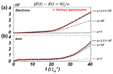
Figure 4: Combinatorial Boltzmann entropy deviations from their initial value normalized to $a$, i.e., $[\mathcal{S}(t)-\mathcal{S}(t=0)]/a$ for (a) electrons and (b) ions. Solid, dashed, and dotted lines are for $a=3.13\times 10^{5},10^{2}$ and 1, respectively. The red diamond symbols indicate the value for the continuous Boltzmann entropy $S$ from Eq. (2).

We perform three simulations that are identical except for the use of different values of $a$. An $a=1$ case has each macro-particle representing a single particle, and we also use values of $a=100$ and the base simulation using $a=3.13\times 10^{5}$. The $a=1$ case warrants further discussion; one could be concerned that there are not enough particles to maintain the plasma approximation. However, that is not the case for our simulations. Our simulations employ $PPG=100$ for each species. The (position space) grid cell in our simulation is about $(2/3)\lambda_{De}$. Thus, these 2D simulations have approximately $(3/2)^{2}\times 100=225$ particles per Debye sphere. This is much larger than 1, as is required for the plasma approximation, and is only a factor of two or so lower than the number of particles per Debye sphere in the MRX experiment and Earth’s ionosphere, as shown in Table 1. Thus, the plasmas being simulated continue to satisfy the plasma approximation, even with $a=1$.

Fig. 4 contains results for the time evolution of the total combinatorial Boltzmann entropy $\mathcal{S}(t)$ integrated over the entire computational domain, shown as a difference from its initial value $S(t=0)$ and divided by $a$, for the three simulations. Panel (a) is for electrons and panel (b) is for ions. The reason to divide by $a$ is that we know from Eq. (35) that the continuous Boltzmann entropy $S$ is directly proportional to $a$ in the limit of large number of particles, so dividing by $a$ allows us to directly compare simulations that use different values of $a$. The red diamonds show the corresponding value of the kinetic entropy from Eq. (2), which follows after employing the Stirling approximation.

First, we note that there is excellent agreement in the large $a$ simulation between the combinatorial $\mathcal{S}$ and continuous $S$ Boltzmann entropies as there should be, which provides additional evidence for the proper implementation of the diagnostic. For the $a=100$ case, a significant difference between the two is observed, especially for the electrons. For the $a=1$ case, the difference is at least an order of magnitude. The results show that if $a$ is not included, or is too low, the combinatorial Boltzmann entropy $\mathcal{S}$ does not agree with the continuous Boltzmann entropy $S$.

To be more specific, a typical maximum value of macro-particles in a phase space bin is approximately 3 in the base simulation. Taking into account the particle weight of $W=0.2/1.44$, analogous to the discussion in Appendix B.1 leading to Eq. (31), for a simulation with $a=100$ implies that there are a maximum of about $3\times(0.2/1.44)\times 100\simeq 40$ actual particles in any phase space bin. The error due to the Stirling approximation for an argument of 40 is about 1%. While this is reasonably good, it represents the minimum error in any cell. Bins with fewer particles contribute higher errors (4 actual particles has a 15% error), leading to the larger errors approaching 30% we see for the $a=100$ simulation. For $a=3.13\times 10^{5}$, the maximum particles per cell is 130,000, for which the error introduced by the Stirling approximation is exceedingly small ($3\times 10^{-4}\%$). This motivates the approximate level of disagreement for the $a=100$ simulation and why the larger $a$ gives good agreement. We note that there are a number of physical systems for which $a$ would be of order 100 for $PPG$ near 100 and a weight of $W=1$, such as Earth’s ionosphere, the MRX reconnection experiment, and high energy density laser plasmas, as seen in Table 1, so there are physical systems for which errors could be introduced by using the Stirling approximation.

Fig. 4 indicates that use of the combinatorial form of the kinetic entropy requires the use of the number of real particles per macro-particle $a$ to get physically appropriate results for real systems. In contrast, the continuous $f\ln f$ form of kinetic entropy does not require inclusion of $a$ to get physical appropriate results. (Fig. 4 also provides validation that the implementation of the $a$ factor in the PIC code was carried out successfully.) A corollary of this is that it would not be appropriate to run a PIC simulation with the idea that macro-particles represent single particles. Instead, one must take into account the fact that macro-particles represent a large number of real particles in physical plasma systems, or one gets a wrong answer for the combinatorial kinetic entropy. Given that the combinatorial version of the kinetic entropy is a perfectly viable approach to calculate the entropy, it is important to make this point here.

IV.5 Dependence on Macro-particles Per Grid Cell ($PPG$)

The limited number of macro-particles in PIC simulations leads to a worse statistical representation of phase space than in the actual system being simulated. Here, we investigate how this impacts the calculation of kinetic entropy by comparing simulations with different numbers of macro-particles per grid cell, keeping the actual number of particles fixed by keeping $a$ times $PPG$ constant. This ensures there are a sufficient number of particles to avoid accuracy issues as discussed in Sec. IV.4. We carry out simulations with $PPG$ of 1, 25, 50, and the base simulation of 100. For $PPG=50,25,$ and 1, we use $a=6.27\times 10^{5}$, $1.25\times 10^{6}$, and $3.13\times 10^{7}$, respectively. The reasons we include a case with $PPG$=1 are (1) some studies have used low $PPG$ in PIC simulations and (2) we can test what happens to the kinetic entropy calculation when the statistics are poor.

Some extra details for the $PPG=1$ case are warranted. Since numerical PIC noise is expected to be significant, we start by performing a simulation with the same divergence cleaning frequency as the other simulations (every 10 particle time steps). We find the time history of the reconnection rate is very different than the higher $PPG$ simulations due to the numerical noise and relatively bad energy conservation. Then, we perform another simulation with divergence cleaning at every time step, which reduces the impact of the noise. The total energy change in this simulation is 7.3%, and the reconnection rate evolution is similar to the higher $PPG$ simulations. We find the magnitude of the kinetic entropy change is similar to the $PPG=1$ case with less frequent divergence cleaning. Consequently, we use the $PPG=1$ simulation with the higher cadence divergence cleaning in what follows.

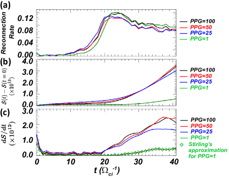
Figure 5: (a) Reconnection rate, (b) deviation of the total combinatorial Boltzmann entropy $\mathcal{S}$ from its initial value, and (c) time rate of change of the total combinatorial Boltzmann entropy $\mathcal{S}$ for simulations with different $PPG$ of 100 (black), 50 (red), 25 (blue), and 1 (green). In (c), the diamonds show the corresponding value using the continuous Boltzmann entropy $S$ instead of the combinatorial Boltzmann entropy $\mathcal{S}$ for the $PPG$=1 case to confirm it is calculated properly.

Fig. 5(a) shows the reconnection rate as a function of time for the four simulations, with the colors defined in the plot and caption. The plot clearly shows that the reconnection rate is quite insensitive to $PPG$, even for a value of $PPG$ = 1 (with additional divergence cleaning). That the reconnection rate can be accurately simulated in PIC simulations with few particles has been previously noted in astrophysical PIC simulation studies of reconnection (Sironi and Spitkovsky, 2014; Sironi, Giannios, and Petropoulou, 2016; Ball, Sironi, and Özel, 2018).

Panel (b) shows the deviation of the combinatorial Boltzmann entropy $\mathcal{S}$ from its initial value for the four simulations with different $PPG$. The $PPG$=1 case deviates from the others significantly, but the results of the other three cases are similar. In order to examine the differences among $PPG$=100, 50 and 25, we further plot the time rate of change of the combinatorial Boltzmann entropy $d\mathcal{S}/dt$ in panel (c). The results for the $PPG$ = 50 and 100 cases are quite similar. This suggests that these numbers for $PPG$ are sufficient to give a relatively stable regime of the kinetic entropy calculation for our simulations.

In contrast, the $PPG=25$ results differ from the higher $PPG$ results, showing that adverse numerical effects from the worse particle statistics take place, especially late in time after reconnection occurs. It is even more dramatic for $PPG=1$, where there is a large discrepancy approaching an order of magnitude. Moreover, a 2D plot of the kinetic entropy density of the $PPG=1$ simulation (not shown) is very similar to the density, as expected, but the departure of the distribution from a Maxwellian has very large noise which swamps out all other structures (since a Maxwellian is not well described by a single macro-particle). These important differences suggest that even though a $PPG$ of 1 can be made to reasonably produce the reconnection rate, one must proceed with caution on matters related to kinetic entropy, including effects such as particle acceleration and plasma heating. A convergence test of kinetic entropy and the effect of small $PPG$ on energization, heating, and energy partitioning would be useful in testing such simulations.

It may seem counter-intuitive that the change of kinetic entropy decreases with fewer $PPG$ since the simulation should be more noisy when $PPG$ is low and one might think this would increase the entropy. However, there is a subtle reason this is not the case, as we can see with an extreme example. Consider a simulation with only a single macro-particle corresponding to $a$ real particles. All $a$ real particles corresponding to that macro-particle are in the same cell in phase space. The kinetic entropy of this macro-particle is equal to that of all $a$ particles in a single cell of phase space (which is zero). Now let time evolve. The macro-particle moves to a new cell in phase space. Since the macro-particle still corresponds to all $a$ particles, all $a$ particles move to the same new cell in phase space. Thus, their contribution to the kinetic entropy at this later time is exactly the same – it is still zero. Consequently, kinetic entropy is perfectly conserved for this simulation even though the number of macro-particles is only 1. Moreover, the low number of macro-particles makes the total entropy smaller than it would be if there were more $PPG$. Thus, a decrease in $PPG$ counter-intuitively leads to a decrease in the change of kinetic entropy despite the increase in particle noise.

IV.6 Dependence on $\Delta v$

While the kinetic entropy should not depend on grid scale for the continuous form in Eqs. (2) and (17), the discrete form in Eq. (16) is required for implementation in PIC and therefore is dependent on the grid scale. Here, we discuss how to choose the size of the velocity space bin size $\Delta v$. The dependence on spatial grid size could be determined using the same approach, but this is left for future work. We choose the optimal $\Delta v$ by comparing simulation results for different $\Delta v$ to analytical results for known Maxwellian distributions at $t=0$ in the base simulation.

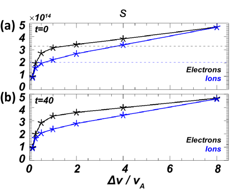
Figure 6: Continuous Boltzmann entropy $S$ for electrons (black) and ions (blue) in seven simulations with $\Delta v/v_{A}=0.125,0.25,0.5,1.0,2.0,4.0,8.0$ (a) at $t=0$ and (b) at $t=40$. The dashed lines in (a) indicate the analytical values at $t=0$ for electrons (black) and ions (blue).

We show results from multiple simulations using velocity bin sizes $\Delta v$ of $0.125,0.25,0.5,1.0,2.0,4.0,$ and 8.0 relative to the ion Alfvén speed $v_{A}$. Fig. 6(a) shows the continuous Boltzmann entropy $S$ at the initial time $t=0$ for both electrons (black) and ions (blue) as a function of the velocity space grid scale $\Delta v$ normalized to the ion Alfvén speed $v_{A}$. As expected, the continuous Boltzmann entropy $S$ of both species increases with $\Delta v$ for sufficiently large values. Below $\Delta v/v_{A}$ of about 0.5 or 1, the variation strongly depends on $\Delta v$.

Also in panel (a) are black and blue horizontal dashed lines corresponding to the analytical prediction of the continuous Boltzmann entropy of electrons and ions, respectively, for the initial conditions from the spatial integral of Eq. (4). By inspection, we see that the numerically calculated value of electron kinetic entropy agrees well with the analytical value for a velocity grid scale just over 1 $v_{A}$. This suggests an appropriate value to use for the velocity space grid of electrons. Similarly, the ion kinetic entropy agrees with the analytical value for a velocity grid just under 1 $v_{A}$. These two results motivated our choice of a grid scale of $\Delta v=1v_{A}$, which is $\approx 0.69\ v_{th,e}$ in terms of the initial electron thermal speed $v_{th,e}$ for this simulation. That this is slightly less than the electron thermal speed is consistent with expectations, as discussed in Appendix B.2. Note, for both electrons and ions, the velocity grid scale that gives best agreement with the analytical calculation is near the species thermal speed ($1.44\ v_{A}$ for electrons, $0.65\ v_{A}$ for ions). Also, the base simulation used the same velocity space grid scale for ions and electrons; this is not a requirement and could be relaxed.

While this approach can be used at $t=0$ when all the distribution functions are Maxwellian and exact solutions are known, there is no assurance that the velocity space grid scale will continue to be sufficient at later times. One way to address this would be to test systems for which the distribution functions are known analytically as a function of time, such as the bump on tail instability (O’neil, 1965; Valentini et al., 2012). We leave such an approach for future work. More generally, given that phase space evolution can lead to very sharp structures in velocity space, this is a very fundamental issue that has previously arisen in Vlasov modeling (Servidio et al., 2015; Camporeale et al., 2016; Roytershteyn and Delzanno, 2018), and it likely has no general solution.

That said, we perform further analysis to assess whether the velocity space resolution adversely impacts our study at later times. First, we note that the temperature (i.e., the spread of the distribution function in velocity space) in this reconnecting system tends to increase in time throughout the domain, so this suggests the resolution at $t=0$ may remain sufficient at later times, at least in these simulations. That this is the case can be seen in Fig. 6(b), which is analogous to panel (a) but at $t=40$. The results are quite similar to those at $t=0$, suggesting only a minor global effect. Indeed, the global change in kinetic entropy is at the 3% level for this simulation.

A more careful approach is to identify the most non-Maxwellian electron distribution in the system at the end of the simulation, $t=41$, and test the effect of the velocity space grid scale in finding its kinetic entropy density. For the base simulation, the most non-Maxwellian distribution occurs at the X-line at late time, when the electrons undergo meandering orbits and produce familiar characteristic distributions like those in Fig. 4 of Ng et al.(Ng et al., 2011) This distribution function has sharp structure and therefore is the hardest to resolve in velocity space, so the error of its kinetic entropy density should be the most.

Using this local distribution in a single grid cell, we calculate the electron kinetic entropy density as a function of velocity space grid scale (not shown), which represents the local counterpart to the global result in Fig. 6. As in the global results, we find that there is a medium range between about $0.5v_{A}$ and $2v_{A}$ where the entropy is not strongly dependent on the velocity space grid. The uncertainty in the kinetic entropy density as a result of the velocity space grid scale is approximately 15%, in spite of the fact that the late time distribution function has structures in velocity space that are not likely to be completely resolved.

The key point to assess this result is that the change in the kinetic entropy between $t$ = 0 and $t$ = 41 is approximately a factor of 2, from about 1.3 (for the electrons far upstream of the current sheet at $t=0$) to about 0.7 (for the meandering electrons at the X-point $t=41$). Thus, the 15% uncertainty introduced by even the worst velocity space grid resolution in our entire simulation is considerably smaller than the physical change in entropy of nearly a factor of 2. This shows that the velocity space grid scale resolution is sufficient for the purposes of this study. However, we emphasize that a careful convergence study is important for future studies and in other plasma applications.

V Discussion and Conclusion

V.1 Summary

This manuscript presents a study of how to implement two forms of the kinetic entropy into fully kinetic particle-in-cell simulations and how to use these quantities to diagnose the physical system. The two forms are the combinatorial Boltzmann entropy $\mathcal{S}=k_{B}\ln\Omega$ and the continuous Boltzmann entropy $S=-k_{B}\int d^{3}rd^{3}vf\ln f$. These forms of kinetic entropy, can be decomposed into a sum of two terms describing the kinetic entropy in position space and velocity space separately.

We then discuss how to implement the diagnostic into PIC simulations, including considerations such as the optimal size of the velocity space grid scale, the number of macro-particles per grid cell, and the number of actual particles per macro-particle. We compare and contrast the merits of each of the two measures of kinetic entropy.

Then, we validate the implementation using two-dimensional in position space, three-dimensional in velocity space collisionless PIC simulations of anti-parallel symmetric magnetic reconnection. The initial conditions contain only drifting Maxwellian distributions which has an analytical solution for the kinetic entropy. This allows for a careful validation of the implementation at the initial time and provides an avenue for optimizing the velocity space grid size. Finally, we discuss the interpretation of the results and how to extract physical understanding from the kinetic entropy.

The results of the present study include the following:

1. The “base” simulation with very low $\Delta t$ demonstrates good conservation of the total kinetic entropy (to 3.2%). The increase in kinetic entropy is purely numerical, but increases monotonically as would be expected for physical collisions and increases faster when reconnection proceeds. The level of increase of kinetic entropy is small enough that simulations with a collision operator should produce entropy at a level high enough to be resolved in future studies.

2. Electrons and ions show different kinetic entropy production rates, with electrons gaining more than ions in the base simulation because their dynamics occurs at smaller scales and therefore are disproportionately impacted by numerical effects.

3. We apply the decomposition of kinetic entropy into position space and velocity space portions to a numerical system and use it to interpret the physics of the system for the first time. Although the total kinetic entropy is nearly conserved, the position and velocity space entropies $S_{{\rm position}}$ and $S_{{\rm velocity}}$ vary noticeably in time. For both electrons and ions, $S_{{\rm position}}$ decreases in time (for most of the simulation), while $S_{{\rm velocity}}$ increases in time. This is physically related to the electrons and ions getting heated during reconnection (increasing their velocity space entropy) and getting compressed (decreasing their position space entropy). This approach will be useful for distinguishing reversible and irreversible dissipation in future studies that incorporate a collision operator, even for distribution functions that are strongly non-Maxwellian.

4. Calculating the combinatorial Boltzmann entropy $\mathcal{S}$ requires specifying the number of actual particles per macro-particle $a$ for the calculation, while the continuous Boltzmann entropy only needs this quantity to convert to real units for comparison with observations or experiments.

5. We show how to choose the number of macro-particles per grid cell $PPG$. For these simulations, a bin size that is close to the electron thermal speed is a good size, and we need at least 50 $PPG$ to get reliable kinetic entropy values for our choice of time step and spatial grid scale. The minimum $PPG$ that is sufficient to reliably calculate the kinetic entropy likely depends on these quantities.

6. We show how to choose the velocity space bin size at the initial time when the simulation has distributions such as Maxwellians for which the entropy is attainable analytically. We find a grid scale slightly smaller than the species thermal speed is a good bin size for our base simulation. There is no clear path for ensuring the velocity space bin size remains adequate for later times because sharp velocity space structures are common in weakly collisional systems. However, for the present study, we have shown that the least resolved distribution at late time introduces only a 15% error in our simulation, far smaller than the physical difference in the kinetic entropy, so the velocity bin resolution is good enough for the purposes of this study. Future work on this issue, for reconnection and for other problems in plasma physics, will be very important.

7. We show that the kinetic entropy is not reliably produced in simulations with a low number of particles per grid, even though the same simulations can be made to reliably produce the reconnection rate. This has important implications about studies of heating and dissipation in systems with few particles per grid cell.

Our study shows that kinetic entropy can serve as a diagnostic of the fidelity of a collisionless PIC code, alongside the often used energy, but also can give key physical insights about the dynamics of a system. The diagnostic developed here should be applicable to any explicit PIC simulation, which should make it useful in many heliospheric, planetary, and astrophysical processes including magnetic reconnection, plasma turbulence, and collisionless shocks. It is useful for systems with distributions with a thermal core and non-thermal tails, but also more broadly for systems with strongly non-Maxwellian distributions.

V.2 Other Insights and Applications

This work provides a number of other insights that are important for applying the kinetic entropy diagnostic for applications. Kinetic entropy in a PIC simulation is sensitive to the phase space bin size, both in position and velocity space. This is because the calculation is discretized on a finite grid. Comparisons between different times in a given simulation, between two different simulations, and between simulations and data should be done with a fixed position and velocity space grid scale to the extent possible.

An interesting result is that one needs to be careful to ensure the bins in phase space have a large number of (actual) particles to obtain accurate kinetic entropy values. Stirling’s approximation is good to within 1% when the number of actual particles in a bin is 40 but has 15% error for 4 actual particles in a bin. Thus, computational and observational studies alike should monitor the number of particles per phase space bin. It is possible in either setting to have insufficient counts to render the Stirling approximation valid. In such cases, the combinatorial Boltzmann entropy $\mathcal{S}$ in Eq. (10) is needed over the continuous Boltzmann entropy $S$ in Eqs. (2) and (17). As discussed in Sec. IV.4, this is the case for some important plasma settings, potentially including laboratory experiments, Earth’s ionosphere, and laser plasmas.

We point out the importance of ensuring a stable regime of the kinetic entropy with the number of numerical macro-particles per grid cell $PPG$. For the base simulation with small time step and well-resolved grid, we find we need at least 50 for $PPG$ to have a stable regime of the kinetic entropy. There have been a number of studies, especially in the plasma astrophysics community, with smaller $PPG$ including as low as 1-4 (Sironi and Spitkovsky, 2014; Sironi, Giannios, and Petropoulou, 2016; Ball, Sironi, and Özel, 2018). We confirm their results that one can get a reasonable reconnection rate in such systems, but for our code the low $PPG$ is insufficient to get a proper kinetic entropy. The Ball, Sironi, and Özel (2018) study tested convergence of particle energy spectra with $PPG$ of 4 and 16; it would be interesting to also check stability of the kinetic entropy diagnostic. We suggest that using kinetic entropy to test for stability for low $PPG$ simulations is a useful technique which is potentially important for studies of particle acceleration and plasma heating in reconnection, turbulence, and shocks.

One challenge for applications is that the conservation of kinetic entropy in ideal (collisionless) systems is only valid for closed, isolated systems. This can easily be accomplished in idealized simulations, but it is unlikely to be the case in naturally occurring systems. The expectation of this line of research is that the dissipation physics can be studied using idealized simulations, and then the insights obtained from the simulations can be compared to real systems. This is already being carried out with data from MMS and will be the subject of future publications.

Another challenge is that typically the continuous Boltzmann entropy density $s=-\int d^{3}vf\ln f$ is mostly proportional to the number density, so a plot of kinetic entropy density by itself is unlikely to reveal any new insights. We will demonstrate in a follow up study that kinetic entropy can be useful for identifying non-Maxwellian distributions for electrons and ions and furthermore that the kinetic entropy can be used to estimate the effective numerical collisionality of a collisionless PIC code.

The initial implementation of the kinetic entropy diagnostic has many ways to be improved, which we outline here. First, our treatment is non-relativistic, but the PIC code in use and many natural systems relevant to study with this tool are relativistic (Kaniadakis, 2009). In addition, comparisons to implicit PIC simulations (which can employ much larger spatial grids and time steps) and Vlasov simulations (which have no PIC noise) would be interesting. More in depth studies into the dependence of the kinetic entropy diagnostic on spatial grid scale and time step would be useful, along with higher macro-particles per grid cell $PPG$. Significant work is needed to choose velocity space bin sizes that do not introduce larger errors after the initial time. Our work used only the linear shape function; it would be interesting to test other shape functions. It would also be interesting to examine kinetic entropy in PIC simulations with open boundary conditions. The present simulations are 2D in position space and 3D in velocity space; simulations that are 3D in both position and velocity space should be carried out. Most importantly, this work employs only collisionless PIC simulations, which means that any dissipation (i.e., any increase of total kinetic entropy) that occurs is through numerical effects. Thus, we are unable to address physical mechanisms for dissipation in the present study. Using a collisional PIC code would allow for an investigation of the physical mechanisms of dissipation with the kinetic entropy diagnostic.

There are also numerous physics topics that are important for future work. Future work should also address parametric studies of kinetic entropy in magnetic reconnection, as well as in plasma turbulence and collisionless shocks. Generalizations to other forms of entropy, such as the Tsallis entropy which describes long-range interactions and contains memory effects (Tsallis, 1988), should also be undertaken. Whether chaotic behavior is sufficient to produce an entropy increase should also be the subject of future work. It is important to see if numerical kinetic entropy production can impact other physical processes like particle acceleration and heating.

Appendix A Theory of Kinetic Entropy

In this section, we discuss the theoretical background of kinetic entropy and its decomposition into position space entropy and velocity space entropy.

A.1 Background on Kinetic Entropy

For a closed system (which in Nature could be thermally insulated, but in a simulation can also be periodic), the form of kinetic entropy $\mathcal{S}$ in a kinetic framework is (Boltzmann, 1877; Planck, 1906)

$$\mathcal{S}(t)=k_{B}\ln\Omega(t),$$ (10)

where $k_{B}$ is Boltzmann’s constant and $\Omega(t)$ is the number of microstates of the system that produce the system’s macrostate at a time $t$. In what follows, we suppress the time dependence to simplify the notation. Each individual plasma species has its own associated kinetic entropy, so there is an implicit subscript $e$ or $i$ for electrons or ions, respectively, that is suppressed for clarity when possible. Following the nomenclature in Frigg and Werndl (2011), we refer to the kinetic entropy in this form as the “combinatorial Boltzmann entropy.” This is one form of kinetic entropy we implement in our PIC code.

To elucidate the meaning of kinetic entropy in this form, consider a plasma with a fixed number of charged particles $N$ for each species. We treat classical, non-relativistic systems (even though the PIC code we use is fully relativistic).

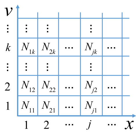
Figure 7: Sketch of phase space $(x,v)$ for a 1D system, discretized into a grid. The number of particles in the bin spanning position $x_{j}$ to $x_{j}+\Delta x$ and velocity $v_{k}$ to $v_{k}+\Delta v$ is $N_{jk}$. This can be suitably extended to higher dimensional systems.

For a three-dimensional (3D) system, phase space is 6D with each particle described by its position and velocity $(\vec{r},\vec{v})$. To calculate kinetic entropy, phase space is discretized into domains we call bins. Fig. 7 shows the discretization of an analogous 1D system. Define $N_{jk}$ as the number of particles in the phase space bin spanning positions $\vec{r}_{j}$ to $\vec{r}_{j}+\Delta\vec{r}$ and velocities $\vec{v}_{k}$ to $\vec{v}_{k}+\Delta\vec{v}$ at a given time $t$, where the components of $\Delta\vec{r}$ and $\Delta\vec{v}$ describe the extent of the bin in each direction in phase space. At this point, we nominally take these bins as finite in size (i.e., not infinitesimal) with an eye to calculating kinetic entropy in PIC simulations. The volumes of the bins in position and velocity space are $\Delta^{3}r$ and $\Delta^{3}v$, respectively. In a 1D system, subscripts $j$ and $k$ signify the bin in position space and velocity space, respectively. In 3D, we continue to use $j$ and $k$ as shorthand to identify the bin, even though we actually need to specify each component of the position and velocity to identify a bin. Thus, we think of $j$ to mean $j_{x},j_{y},j_{z}$ for the $x$,$y$,$z$ directions in position space and $k$ to mean $k_{x},k_{y},k_{z}$ for the $v_{x}$,$v_{y}$,$v_{z}$ directions in velocity space. By definition,

$$N=\sum_{j,k}N_{jk}.$$ (11)

A given macrostate is defined by the collection of all the $N_{jk}$, which via integration yields all the fluid quantities of the system. A microstate is a possible way to choose the particles in the system to produce a given macrostate, treating individual particles classically as distinguishable.

Using this construct, the number $\Omega$ of possible microstates for a given macrostate is calculated using combinatorics (Bellan, 2008); it is the number of permutations that produce the macrostate with $N_{jk}$ particles in the $jk$th cell by swapping individual distinguishable particles between any of the bins, i.e.,

$$\Omega=\frac{N!}{\prod_{j,k}N_{jk}!}.$$ (12)

Inserting this expression into Eq. (10) and simplifying gives the combinatorial Boltzmann entropy $\mathcal{S}$ in terms of the $N_{jk}$:

$$\mathcal{S}=k_{B}\left[\ln N!-\sum_{j,k}\ln N_{jk}!\right].$$ (13)

The first term is a constant assuming the total number of particles $N$ in the closed system is fixed. Since only changes in entropy are physically important, we can drop the first term if desired (though we retain it in the calculation of the combinatorial Boltzmann entropy in our PIC simulations). Note, however, that whether the first term is retained or not, quantities like percentage changes in entropy should be calculated solely relative to the second term.

It is common to approximate Eq. (13) using Stirling’s approximation $\ln N_{jk}!\approx N_{jk}\ln N_{jk}-N_{jk}$, which is valid when $N_{jk}\gg 1$, as is typically the case but may have exceptions. A short calculation using Eq. (11) yields

$$S=k_{B}\left[N\ln N-\sum_{j,k}N_{jk}\ln N_{jk}\right],$$ (14)

where we write the approximate entropy as $S$ instead of $\mathcal{S}$. For use in a kinetic description of a fluid or plasma, one writes the kinetic entropy in terms of the distribution function $f(\vec{r},\vec{v})$. The distribution function at position $\vec{r}_{j}$ and velocity $\vec{v}_{k}$ is approximated as

$$f(\vec{r}_{j},\vec{v}_{k})\approx\frac{N_{jk}}{\Delta^{3}r\Delta^{3}v}.$$ (15)

Replacing $N_{jk}$ in Eq. (14) with this expression and simplifying gives

$$S= k_{B} \left[N\ln\left(\frac{N}{\Delta^{3}r\Delta^{3}v}\right)\right.$$ (16)

$$\left.-\sum_{j,k}(\Delta^{3}r\Delta^{3}v)f(\vec{r}_{j},\vec{v}_{k})\left[\ln f(\vec{r}_{j},\vec{v}_{k})\right]\right].$$

As in Eq. (13), the first term is a constant (for a fixed phase space bin size) and can be discarded. In the limit in which $\Delta\vec{r}$ and $\Delta\vec{v}$ are small, the second term yields the commonly used form of the kinetic entropy

$$S=-k_{B}\int d^{3}{r}d^{3}vf(\vec{r},\vec{v})\left[\ln f(\vec{r},\vec{v})\right],$$ (17)

where $d^{3}r$ and $d^{3}v$ are the infinitesimal spatial and velocity space volumes. Following the nomenclature of Frigg and Werndl (2011), we refer to Eq. (17) as the “continuous Boltzmann entropy” to distinguish it from the combinatorial Boltzmann entropy $\mathcal{S}$. This is the second form of kinetic entropy we implement in our PIC code. Note that in dropping the first term of Eq. (16), there is an issue with the units of $S$ in that the second term is no longer formally dimensionless. Therefore, care is necessary when the continuous Boltzmann entropy is desired in proper units. We discuss this in more detail in Appendix B.4.

We note in passing that one can alternately normalize $f$ to be a probability density rather than a phase space density. In this convention, the entropy would be related to the Shannon entropy and information theory (Shannon, 1948; Jaynes, 1963). We do not employ this convention here with an eye to experiments and observations that directly measure distribution functions.

The continuous Boltzmann entropy density, i.e., the continuous Boltzmann entropy per unit volume, is denoted by $s(\vec{r})$ and given by

$$s(\vec{r})=-k_{B}\int d^{3}vf(\vec{r},\vec{v})\left[\ln f(\vec{r},\vec{v})\right].$$ (18)

We point out that the continuous Boltzmann entropy density $s_{M}(\vec{r})$ for a 3D drifting Maxwellian distribution in local thermodynamic equilibrium (LTE) for a species of mass $m$, number density $n(\vec{r})$, bulk flow velocity $\vec{u}(\vec{r})$, and temperature $T(\vec{r})$, with $f(\vec{r},\vec{v})=f_{M}=n(\vec{r})[m/2\pi k_{B}T(\vec{r})]^{3/2}e^{-m[\vec{v}-\vec{u}(\vec{r})]^{2}/2k_{B}T(\vec{r})}$, is exactly solvable with

$$s_{M}(\vec{r})=\frac{3}{2}k_{B}n(\vec{r})\left[1+\ln\left(\frac{2\pi k_{B}T(\vec{r})}{mn^{2/3}(\vec{r})}\right)\right].$$ (19)

This result shows the fluid entropy per particle $s/n$ is related to $p/\rho^{\gamma}$, where $p=nk_{B}T$ is the (scalar) pressure, $\rho=mn$ is the mass density, and $\gamma=5/3$ is the ratio of specific heats. In an adiabatic process, conservation of $s/n$ is synonymous with conservation of $p/\rho^{\gamma}$, which is typically used in fluid models. Equation (19) is useful for validating the implementation of the kinetic entropy diagnostic into kinetic codes.

A.2 Decomposition of Kinetic Entropy into Position and Velocity Space Entropies

Boltzmann’s kinetic entropy is defined in terms of permutations of particles with any position and velocity in phase space. It is tempting to interpret the kinetic entropy density in Eq. (18) as the entropy purely associated with permuting particles in velocity space, but this is only correct if the plasma density is uniform. If the density is non-uniform (i.e., $n$ is a function of $\vec{r}$), it has been shown that the total kinetic entropy can be decomposed into a sum of a position space entropy and a velocity space entropy (Mouhot and Villani, 2011; Goldstein and Lebowitz, 2004), as we now review.

By adding and subtracting a common term in Eq. (13), $k_{B}\sum_{j}\ln N_{j}!$, where $N_{j}=\sum_{k}N_{jk}$ is the total number of particles in spatial cell $j$, i.e., with any velocity, the combinatorial Boltzmann entropy $\mathcal{S}$ can be written as

$$\mathcal{S} = k_{B}\left[\ln N!-\sum_{j}\ln N_{j}!\right]$$ (20)

$$+ k_{B}\sum_{j}\left[\ln N_{j}!-\sum_{k}\ln N_{jk}!\right].$$

The first two terms have the same form as Eq. (13), except that the second term has $N_{j}!$ instead of $N_{jk}!$, so they are defined as the position space kinetic entropy,

$$\mathcal{S}_{\text{position}}=k_{B}\left[\ln N!-\sum_{j}\ln N_{j}!\right].$$ (21)

Similarly, the last two terms in Eq. (20) have the same form as Eq. (13) with $N$ replaced by $N_{j}$ and the summation being only over velocity space, so they are defined as the velocity space kinetic entropy

$$\mathcal{S}_{\text{velocity}}=\sum_{j}k_{B}\left[\ln N_{j}!-\displaystyle\sum_{k}\ln N_{jk}!\right].$$ (22)

Consequently, Eq. (20) can be written as

$$\mathcal{S}=\mathcal{S}_{\text{position}}+\mathcal{S}_{\text{velocity}},$$ (23)

so the combinatorial Boltzmann entropy is decomposed into a sum of position space kinetic entropy and velocity space kinetic entropy.

Note that there is an asymmetry between the treatment of position and velocity space in this definition of the position space entropy and velocity space entropy. The number of microstates per macrostate is calculated in velocity space for each spatial cell to obtain velocity space entropy, while the position space entropy is obtained by summing over velocity space first. Alternatively, one could interchange the treatment of position and velocity space in this calculation. Therefore, the decomposition used here is not unique. However, the decomposition employed here and elsewhere gives meaningful information about local velocity space entropy changes that are indicative of heating or dissipation, which makes it a preferred decomposition.

As in Appendix A.1, one can readily derive expressions for the position and velocity space kinetic entropies in terms of the distribution function and analogous expressions in terms of the plasma density $n$; using Stirling’s approximation assuming there are a large number of particles, one obtains the discrete forms of the continuous Boltzmann position and velocity space kinetic entropies as

$$S_{\text{position}} = k_{B}\left[N\ln\left(\frac{N}{\Delta^{3}r}\right)\right.$$ (24)

$$- \left.\sum_{j}(\Delta^{3}r)n(\vec{r}_{j})\ln n(\vec{r}_{j})\right],$$

$$S_{\text{velocity}} \equiv \sum_{j}(\Delta^{3}r)s_{\text{velocity}}(\vec{r}_{j}),$$ (25)

$$s_{\text{velocity}}(\vec{r}_{j}) = k_{B}\left[n(\vec{r}_{j})\ln\left(\frac{n(\vec{r}_{j})}{\Delta^{3}v}\right)\right.$$ (26)

$$- \left.\sum_{k}(\Delta^{3}v)f(\vec{r}_{j},\vec{v}_{k})\ln f(\vec{r}_{j},\vec{v}_{k})\right],$$

where $n(\vec{r}_{j})=N_{j}/\Delta^{3}r$ is the number density at spatial cell $j$. Expressions in terms of continuous variables come from taking the limit of small bin size gives

$$S_{\text{position}} = k_{B}\left[N\ln\left(\frac{N}{\Delta^{3}r}\right)\right.$$ (27)

$$- \left.\int d^{3}rn(\vec{r})\ln n(\vec{r})\right],$$

$$S_{\text{velocity}} \equiv \int d^{3}rs_{\text{velocity}}(\vec{r}),$$ (28)

$$s_{\text{velocity}}(\vec{r}) = k_{B}\left[n(\vec{r})\ln\left(\frac{n(\vec{r})}{\Delta^{3}v}\right)\right.$$ (29)

$$- \left.\int d^{3}vf(\vec{r},\vec{v})\ln f(\vec{r},\vec{v})\right].$$

Note, the second term in $s_{\text{velocity}}(\vec{r})$ is merely $s(\vec{r})$ from Eq. (18), so the two differ by the first term. The key point is that the kinetic entropy density $-k_{B}\int d^{3}vf\ln f$ is not the velocity space entropy because of this extra term. Only in the limit in which $n(\vec{r})$ is uniform are the two effectively the same. .

The physical meaning of the position and velocity space entropies are given by analogies with the combinatorial Boltzmann entropy $\mathcal{S}$. The position space entropy describes the entropy arising from permutations of particles in position space without regard to their velocity. For example, there is only one way to have all the particles in a single bin in position space; $\Omega=1$ for that system and the position space entropy is zero. In contrast, a uniform density has the largest number of microstates that produce that macrostate, so it is the configuration with the largest position space entropy. Therefore, compressing a plasma increases the local density, so is associated with a local decrease in position space entropy.

The velocity space entropy has a similar interpretation – it is the entropy associated with the permutation of particles in velocity space at a fixed cell in phase space, then summed over all spatial bins. As with the position space entropy, more distributed particles in velocity space are associated with higher velocity space entropy, while sharper (colder) distributions have lower velocity space entropies. Increases in density and temperature both lead to an increase in velocity space entropy, as is seen explicitly for a Maxwellian distribution in Eq. (19). Note, for an adiabatic process for a system in local thermodynamic equilibrium, the total entropy is conserved. However, the position and velocity space entropies can change, with kinetic entropy converted between them. During adiabatic compression, for example, the position space entropy decreases as described above. This decrease is perfectly balanced by adiabatic heating which increases the velocity space entropy. We find the decomposition into position and velocity space entropies provides useful insights in the analysis of the PIC simulations.

Appendix B Implementation of Kinetic Entropy Diagnostic in PIC Simulations

Table 1: Representative values of the plasma parameter $n\lambda_{De}^{3}$ in a number of plasma settings (Ji and Daughton, 2011; Rosenberg et al., 2015; Naval Research Laboratory Plasma Physics Division, 2018).

Setting	Density $({\rm cm}^{-3})$	$T_{e}$ (eV)	$n\lambda_{De}^{3}$
Solar active region	$10^{9}$	100	$1.3\times 10^{7}$
Magnetotail	0.2	500	$1.0\times 10^{13}$
MRX reconnection experiment	(0.1 - 1) $\times 10^{14}$	5-15	450-7,000
Solar wind at 1 AU	10	10	$4.1\times 10^{9}$
Magnetosheath	20	50	$3.2\times 10^{10}$
Earth’s ionosphere	$10^{6}$	0.01-0.1	410-13,000
High energy density laser plasma	$10^{20}$	1000	1,300

In this section, we provide a detailed summary of how we implement the kinetic entropy diagnostic into our PIC code p3d (Zeiler et al., 2002), although the approach should be applicable to any explicit PIC code. We emphasize that we use periodic boundary conditions so that the system is closed and one can unambiguously determine if there are global changes in kinetic entropy (as opposed to open systems where the kinetic entropy can change via dynamics at the boundary). In what follows, we break down the procedure into steps and discuss each in turn.

B.1 Macro-particles vs. Actual Particles

As discussed in Appendix A.1, calculating the combinatorial $\mathcal{S}$ or continuous $S$ Boltzmann entropies requires a knowledge of the number of particles in each cell in phase space. In a PIC simulation, the “particles” are actually macro-particles, each representing a chunk of phase space containing a large number of actual particles. Therefore, there is a difference between the number of particles and number of macro-particles in each cell. As we show here, the relative structure of the continuous Boltzmann entropy $S$ is not sensitive to this difference. However, when converting $S$ from a PIC simulation into real units, the results are sensitive to this difference. Moreover, the combinatorial Boltzmann entropy $\mathcal{S}$ is sensitive to the number of actual particles represented by each macro-particle.

Here, we discuss how to relate the number of macro-particles to the number of actual particles. We define a constant $a$ as the number of actual particles per macro-particle. The approach to estimate $a$ is to find the number of actual particles, say, electrons, that would be in a given grid cell in the simulation. For a system with a known number density $n$, the number of electrons $N_{cell}$ in a spatial volume $\Delta^{3}r$ corresponding to a grid cell in PIC is

$$N_{cell}\sim n\Delta^{3}r.$$ (30)

A typical grid size for an explicit PIC simulation is close to the electron Debye length $\lambda_{De}=(\epsilon_{0}k_{B}T_{e}/n_{e}e^{2})^{1/2}$. Thus, $N_{cell}$ is on a similar scale as the plasma parameter $n\lambda_{De}^{3}$. For reference, representative values for the plasma parameter in various settings are provided in Table 1, though of course these are merely representative and may differ for particular applications.

To get a comparable number for the PIC code in order to find $a$, we note that many PIC codes, including the one in use here, allow for macro-particles to be assigned a different weight $W$, which improves the statistics in systems with non-uniform initial densities. This must be accounted for in the estimation of $N_{cell}$. We now estimate $N_{cell}$ using the initial conditions of the simulations carried out for the present study. At $t=0$ in our simulations, $W$ is same for all macro-particles in each grid cell and is proportional to the local density. Thus, $PPG\times W$ represents the effective number of macro-particles per grid cell, so at $t=0$ the number of actual particles in a cell is

$$N_{cell}=PPG\times W\times a.$$ (31)

Equating the two expressions for $N_{cell}$ from Eqs. (30) and (31) gives

$$a=\frac{n\Delta^{3}r}{PPG\times W}.$$ (32)

In simulations for which $W$ is not a constant for all particles in each cell, a generalization of this approach is necessary.

It is important to note when and how including $a$ is necessary in calculating kinetic entropy. Define $\mathcal{N}_{jk}$ as the number of weighted macro-particles in the $jk$th bin in phase space; then

$$N_{jk}=a\mathcal{N}_{jk}.$$ (33)

The value for $\mathcal{N}_{jk}$ is what one gets from the code when counting weighted macro-particles, but does not take into account the number of actual particles per macro-particle. Physically, because the limited number of macro-particles in a PIC simulation implies that there is a small number of macro-particles per phase space bin, the number of permutations of the macro-particles is much smaller than the number of permutations of actual particles. Therefore, if one uses $\mathcal{N}_{jk}$ instead of $N_{jk}$ to calculate Eq. (13), the result is much smaller than that of actual system. More importantly, the Stirling approximation and thus the continuous Boltzmann entropy $S$ definition would be invalid since $\mathcal{N}_{jk}$ is small. The importance of including $a$ can be seen analytically, as well. Writing Eq. (13) in terms of $\mathcal{N}_{jk}$ gives $\mathcal{S}=k_{B}[\ln(a\mathcal{N})!-\sum_{j,k}\ln(a\mathcal{N}_{jk})!]$, which is not equal to $ak_{B}[\ln\mathcal{N}!-\sum_{j,k}\ln\mathcal{N}_{jk}!]$. Thus, the value for $a$ must be included at calculation time to get the proper value of the combinatorial Boltzmann entropy $\mathcal{S}$.

In contrast, the kinetic entropy (i.e., after using the Stirling approximation) is simply linear in $a$. Using $N=a\mathcal{N}$ and $N_{jk}=a\mathcal{N}_{jk}$ in Eq. (14) gives

$$S=k_{B}\left[a\mathcal{N}\ln(a\mathcal{N})-\sum_{j,k}a\mathcal{N}_{jk}\ln(a\mathcal{N}_{jk})\right].$$ (34)

Carrying out simple manipulations gives

$$S=ak_{B}\left[\mathcal{N}\ln\mathcal{N}-\sum_{j,k}\mathcal{N}_{jk}\ln\mathcal{N}_{jk}\right].$$ (35)

Thus, one can simply calculate the continuous Boltzmann entropy using macro-particles in the simulation, and then scale the result by $a$ to get a value for $S$. The same result holds for the forms in terms of the distribution function $f$ [i.e., Eq. (17) and (18)]. In other words, if comparing $f$ or $S$ between a PIC simulation and observations or experiments and an absolute comparison is desired, one must multiply the raw $f$ and $S$ from the simulation by $a$ to convert it to a physical result.

B.2 Binning Macro-Particles in Phase Space

In order to obtain the distribution function, one has to discretize phase space (with bins from $\vec{r}_{j},\vec{v}_{k}$ to $\vec{r}_{j}+\Delta\vec{r},\vec{v}_{k}+\Delta\vec{v}$) and calculate the contribution of each macro-particle to every phase space bin. There are numerous approaches to representing the number density of a macro-particle in a PIC code, referred to as its shape (Birdsall and Langdon, 2004). The approach used in p3d, and therefore applied here, is a linear shaping function that assumes the charge density from each macro-particle drops linearly from its maximum to zero a distance one spatial grid cell away in each direction. Therefore, in any PIC simulation without a $\delta$-function shaping function, a macro-particle contributes to the density in each of the surrounding cells. To calculate kinetic entropy, we use the same shape function for each particle in velocity space (i.e., linear). Therefore, the number of macro-particles in a phase space bin at any given time is typically not an integer. We suggest that the implementation of the kinetic entropy calculation should employ the same particle shape as what is employed in the code in use, but leave further investigation to future work.

Here is the procedure we use for determining the number of macro-particles in each phase space bin:

• Without using the kinetic entropy diagnostic, optimize the numerical parameters on a test simulation to ensure proper spatial and temporal resolution. Using the output from this simulation, find the maximum speed $v_{max}$ among all macro-particles for all times, which should be $\ll c$ in the non-relativistic limit. Then, the range of velocity space to be discretized is restricted to $[-v_{max},v_{max}]$. We use the same velocity range for each velocity component and for all time. (One could choose $v_{max}=c$ without doing a test simulation first, but for non-relativistic systems one would have many phase space cells with no particles, which leads to wasted memory and longer computational times for fixed velocity space bin size.)

• Discretize velocity space by defining a velocity bin size $\Delta v$, which we choose to be the same in each direction in velocity space. The velocity space bin size should be small enough to resolve typical velocity distribution functions, but large enough to preserve reasonably good statistics without many bins lacking particles, which leads to longer computational times. If the velocity distributions in a system have known theoretical kinetic entropy values, a good way to determine $\Delta v$ is to compare the results using different $\Delta v$ with the predicted values, as we discuss further in Sec. IV.6. We find that using a velocity space bin size comparable to the thermal speed is a good choice for the parameters of our simulation.

  Since $\Delta v$ determines the constant terms in Eqs. (16), (26) and (29), an absolute comparison of kinetic entropies of species with different $\Delta v$ would not be meaningful. Instead, only relative changes to kinetic entropy should be used in such a case. Therefore, for this initial study, we choose parameters so that the ion and electron thermal speeds are comparable, so we can use the same $\Delta v$ for both electrons and ions and be able to make direct comparisons. For systems for which $v_{th,e}$ and $v_{th,i}$ are different, one should use different bin sizes for each species. It is important to note that once the velocity space bin size for each species is set, it should be held fixed for the duration of the simulation and should be the same size for all grid cells. These constraints are necessary to be able to compare kinetic entropies at different times and at different locations.

• Choose a spatial bin size $\Delta x$. In principle, this need not be the same as the grid scale $\Delta x$, but this is the most logical choice and what we employ here.

• Cycle over every macro-particle and find the number density contribution to each spatial bin using the particle shape in the code, and increment its contribution to the number of macro-particles in the appropriate phase space bin based on the three components of the macro-particle’s velocity. The end result after counting all macro-particle contributions to every phase space bin is the total number of macro-particles in every bin $\mathcal{N}_{jk}$. Recall, this typically is not an integer.

• If one wants to calculate the combinatorial Boltzmann entropy $\mathcal{S}$, then multiply $\mathcal{N}_{jk}$ in each bin by $a$ to get $N_{jk}$. As discussed in Appendix B.1, multiplying by $a$ at calculation time is not necessary for the continuous Boltzmann entropy $S$, but it would lead to an incorrect value of the combinatorial Boltzmann entropy $\mathcal{S}$.

Spatial cells at the boundary of a computational domain need to get information from other processors for macro-particles in nearby cells that contribute to $N_{jk}$. This leads to an increase in run time; for the present study, the “base” simulation takes $13\%$ more time than the same simulation without calculating the kinetic entropy. We believe this performance could be improved, but leave that for future work.

B.3 Calculating Distribution Functions and Kinetic Entropies

The distribution function $f(\vec{r}_{j},\vec{v}_{k})$ at bin $\vec{r}_{j}$ and $\vec{v}_{k}$ is immediately approximated from $N_{jk}$ using Eq. (15). Once $f$ is obtained for all velocity space bins in all spatial cells, the forms of continuous Boltzmann entropy are readily calculated, such as Eq. (16) for $S$, the discretized version of Eq. (18) for $s(\vec{r}_{j})=-k_{B}\sum_{k}(\Delta^{3}v)f(\vec{r}_{j},\vec{v}_{k})\ln[f(\vec{r}_{j},\vec{v}_{k})]$, and Eq. (26) for $s_{\text{velocity}}$. Note $S_{\text{position}}$ in Eq. (24) does not require the distribution function.

To find the combinatorial Boltzmann entropy $\mathcal{S}$, use Eq. (13). Since the $N_{jk}$ are not integers, the factorial in Eq. (13) needs to be reinterpreted using the $\Gamma$ function for which $\Gamma(N+1)=N!$ for integer $N$ (Arfken and Weber, 1995) as

$$\mathcal{S}=k_{B}\left[\ln[\Gamma(N+1)]-\sum_{j,k}\ln[\Gamma(N_{jk}+1)]\right].$$ (36)

Note that $N_{jk}$ need not be large in every cell, so the non-integer part should not be ignored. Fortuitously, many programming languages contain an intrinsic function for $\ln[\Gamma(x)]$, so the calculation is efficient and there are no issues with performing this calculation for large argument [while calculating $\Gamma(N+1)$ separately would lead to numerical problems for large arguments]. A similar calculation can be used to get the combinatorial Boltzmann entropy for position and velocity space from Eqs. (21) and (22), respectively.

B.4 Merits of Combinatorial vs. Continuous Boltzmann Entropy

We close this section with a discussion of the relative merits between the combinatorial $\mathcal{S}$ and continuous $S$ Boltzmann kinetic entropies. Three advantages of the combinatorial Boltzmann entropy are that it is the most accurate form of kinetic entropy (it does not rely on assuming $N_{jk}\gg 1$), it is automatically in appropriate units, and the intrinsic lngamma function in many coding languages makes the calculations efficient and more importantly can be calculated for large argument, whereas a direct calculation taking the factorial of a large number is not possible. A drawback of the combinatorial Boltzmann entropy is that the value of $a$, describing the number of actual particles per macro-particle, must be included from the beginning in the calculation. Thus, if one wants to see how the combinatorial Boltzmann entropy changes between two different values of $a$, one must redo the calculation of kinetic entropy with a different $a$ value.

The continuous Boltzmann entropy $S$ has the advantage that one does not need to specify $a$ at run-time. Therefore, finding the kinetic entropy for the same simulation but with a different $a$ is trivial and does not require redoing the calculation. A disadvantage of the continuous Boltzmann entropy is that one has to make sure that $a$ is large enough that the errors in Stirling’s approximation are small, which is discussed further in Sec. IV.4. Another disadvantage is that the results are not in appropriate units because the argument of the natural logarithm in $S=-k_{B}\int d^{3}rd^{3}vf\ln f$ from Eq. (17) is not dimensionless. This comes about because a term is dropped from Eq. (16), and the dropped term contains information about the units inside the natural log. So, to convert the simulated continuous Boltzmann entropy to real units for comparison to observations or experiments, one must either (a) include the dropped term or (b) choose a reference value of continuous Boltzmann entropy at a particular location and time and present all values as a change in kinetic entropy relative to that reference. This enforces that the quantities have the appropriate units.

References

- Hesse et al. (2011) M. Hesse, T. Neukirch, K. Schindler, M. Kuznetsova, and S. Zenitani, “The diffusion region in collisionless magnetic reconnection,” Space Sci. Rev. 160, 3 (2011).
- Cassak (2016) P. A. Cassak, “Inside the black box: Magnetic reconnection and the magnetospheric multiscale mission,” Space Weather 14, 186 (2016).
- Drake et al. (2006) J. F. Drake, M. Swisdak, K. M. Schoeffler, B. N. Rogers, and S. Kobayashi, “Formation of secondary islands during magnetic reconnection,” Geophys. Res. Lett. 33, L13105 (2006).
- Cranmer (2002) S. R. Cranmer, “Coronal holes and the high-speed solar wind,” Space Sci. Rev. 101, 229 (2002).
- Parashar et al. (2009) T. N. Parashar, M. A. Shay, P. A. Cassak, and W. H. Matthaeus, “Kinetic dissipation and anisotropic heating in a turbulent collisionless plasma,” Phys. Plasmas 16, 032310 (2009).
- Howes (2018) G. G. Howes, “Laboratory space physics: Investigating the physics of space plasmas in the laboratory,” Phys. Plasmas 25, 055501 (2018).
- Krall (1997) N. A. Krall, “What do we really know about collisionless shocks?” Adv. Space Res. 20, 715 (1997).
- Reynolds (2008) S. P. Reynolds, “Supernova remnants at high energy,” Ann. Rev. Astron. Astrophys. 46, 89 (2008).
- Beall (2014) J. H. Beall, “A review of astrophysical jets,” Acta Polytechnica CTU Proceedings 1, 259 (2014).
- Gaensler and Slane (2006) B. M. Gaensler and P. O. Slane, “The evolution and structure of pulsar wind nebulae,” Ann. Rev. Astron. Astrophys. 44, 17 (2006).
- Draine and McKee (1993) B. T. Draine and C. F. McKee, “Theory of interstellar shocks,” Annual review of astronomy and astrophysics 31, 373–432 (1993).
- Enßlin et al. (1998) T. A. Enßlin, P. L. Biermann, U. Klein, and S. Kohle, “Cluster radio relics as a tracer of shock waves of the large-scale structure formation,” Astron. Astrophys. 332, 395 (1998).
- Priest and Forbes (2002) E. R. Priest and T. R. Forbes, “The magnetic nature of solar flares,” Astron. Astrophs. Rev. 10, 313–377 (2002).
- Klimchuk (2006) J. A. Klimchuk, “On solving the coronal heating problem,” Solar Phys. 234, 41–77 (2006).
- Gosling (2007) J. T. Gosling, “Encyclopedia of the solar wind,” (Elsevier, 2007) Chap. 12.
- Kivelson and Russell (1995) M. G. Kivelson and C. T. Russell, eds., Introduction to Space Physics (Cambridge University Press, 1995).
- Tsurutani and Stone (2013) B. T. Tsurutani and R. G. Stone, eds., Collisionless Shocks in the Heliosphere: Reviews of Current Research, Volume 35, Geophysical Monograph Series (American Geophysical Union, 2013).
- Burch et al. (2016a) J. L. Burch, T. E. Moore, R. B. Torbert, and B. L. Giles, “Magnetospheric multiscale overview and science objectives,” Space Sci. Rev. 199, 5 (2016a).
- Burch et al. (2016b) J. L. Burch, R. B. Torbert, T. D. Phan, L.-J. Chen, T. E. Moore, R. E. Ergun, J. P. Eastwood, D. J. Gershman, P. A. Cassak, M. R. Argall, S. Wang, M. Hesse, C. J. Pollock, B. L. Giles, R. Nakamura, B. H. Mauk, S. A. Fuselier, C. T. Russell, R. J. Strangeway, J. F. Drake, M. A. Shay, Y. V. Khotyaintsev, P.-A. Lindqvist, G. Marklund, F. D. Wilder, D. T. Young, K. Torkar, J. Goldstein, J. C. Dorelli, L. A. Avanov, M. Oka, D. N. Baker, A. N. Jaynes, K. A. Goodrich, I. J. Cohen, D. L. Turner, J. F. Fennell, J. B. Blake, J. Clemmons, M. Goldman, D. Newman, S. M. Petrinec, K. J. Trattner, B. Lavraud, P. H. Reiff, W. Baumjohann, W. Magnes, M. Steller, W. Lewis, Y. Saito, V. Coffey, and M. Chandler, “Electron-scale measurements of magnetic reconnection in space,” Science 352, 6290 (2016b).
- Servidio et al. (2017) S. Servidio, A. Chasapis, W. Matthaeus, D. Perrone, F. Valentini, T. Parashar, P. Veltri, D. Gershman, C. Russell, B. Giles, et al., “Magnetospheric multiscale observation of plasma velocity-space cascade: Hermite representation and theory,” Physical review letters 119, 205101 (2017).
- Chen, Klein, and Howes (2019) C. Chen, K. Klein, and G. Howes, “Evidence for electron landau damping in space plasma turbulence,” Nature communications 10, 740 (2019).
- Chen et al. (2018) L.-J. Chen, S. Wang, L. B. Wilson, S. Schwartz, N. Bessho, T. Moore, D. Gershman, B. Giles, D. Malaspina, F. D. Wilder, R. E. Ergun, M. Hesse, H. Lai, C. Russell, R. Strangeway, R. B. Torbert, A. F.-Vinas, J. Burch, S. Lee, C. Pollock, J. Dorelli, W. Paterson, N. Ahmadi, K. Goodrich, B. Lavraud, O. Le Contel, Y. V. Khotyaintsev, P.-A. Lindqvist, S. Boardsen, H. Wei, A. Le, and L. Avanov, “Electron bulk acceleration and thermalization at earth’s quasiperpendicular bow shock,” Phys. Rev. Lett. 120, 225101 (2018).
- Vaivads et al. (2016) A. Vaivads, A. Retinó, J. Soucek, Y. V. Khotyaintsev, F. Valentini, C. P. Escoubet, O. Alexandrova, M. André, S. D. Bale, M. Balikhin, and et al., “Turbulence heating observer - satellite mission proposal,” Journal of Plasma Physics 82, 905820501 (2016).
- Shay, Drake, and Swisdak (2007) M. A. Shay, J. F. Drake, and M. Swisdak, “Two-scale structure of the electron dissipation region during collisionless magnetic reconnection,” Phys. Rev. Lett. 99, 155002 (2007).
- Zenitani et al. (2011) S. Zenitani, M. Hesse, A. Klimas, and M. Kuznetsova, “New measure of the dissipation region in collisionless magnetic reconnection,” Phys. Rev. Lett. 106, 195003 (2011).
- Swisdak (2016) M. Swisdak, “Quantifying gyrotropy in magnetic reconnection,” Geophys. Res. Lett. 43, 43 (2016).
- Ashour-Abdalla et al. (2016) M. Ashour-Abdalla, G. Lapenta, R. Walker, M. El-Alaoui, H. Liang, M. Zhou, J. Berchem, and M. L. Goldstein, “Identifying the electron diffusion region in a realistic simulation of earth’s magnetotail,” Geophysical Research Letters 43, 6005–6011 (2016).
- Sitnov et al. (2018) M. I. Sitnov, V. G. Merkin, V. Roytershteyn, and M. Swisdak, “Kinetic dissipation around a dipolarization front,” Geophys. Res. Lett. 45, 4639 (2018).
- Wan et al. (2016) M. Wan, W. H. Matthaeus, V. Roytershteyn, T. N. Parashar, P. Wu, and H. Karimabadi, “Intermittency, coherent structures and dissipation in plasma turbulence,” Physics of Plasmas 23, 042307 (2016).
- Yang et al. (2017a) Y. Yang, W. H. Matthaeus, T. N. Parashar, P. Wu, M. Wan, Y. Shi, S. Chen, V. Roytershteyn, and W. Daug hton, “Energy transfer channels and turbulence cascade in vlasov-maxwell turbulence,” Phys. Rev. E 95, 061201 (2017a).
- Yang et al. (2017b) Y. Yang, W. H. Matthaeus, T. N. Parashar, C. C. Haggerty, V. Roytershteyn, W. Daughton, M. Wan, Y. Shi, and S. Chen, “Energy transfer, pressure tensor, and heating of kinetic plasma,” Physics of Plasmas 24, 072306 (2017b).
- Boltzmann (1877) L. Boltzmann, “Über die beziehung dem zweiten haubtsatze der mechanischen wärmetheorie und der wahrscheinlichkeitsrechnung resp. dem sätzen über das wäarmegleichgewicht,” Wiener Berichte 76, 373–435 (1877), in (Boltzmann 1909) Vol. II, paper 42.
- Bellan (2008) P. M. Bellan, Fundamentals of Plasma Physics (Cambridge University Press, 2008).
- Erickson and Wolf (1980) G. M. Erickson and R. A. Wolf, “Is steady convection possible in the earth’s magnetotail?” Geophys. Res. Lett. 7, 897 (1980).
- Borovsky et al. (1998) J. E. Borovsky, M. F. Thomsen, R. C. Elphic, T. E. Cayton, and D. J. McComas, “The transport of plasma sheet material from the distant tail to geosynchronous orbit,” J. Geophys. Res. 103, 20,297 (1998).
- Kaufmann and Paterson (2006) R. L. Kaufmann and W. R. Paterson, “Magnetic flux and particle transport in the plasma sheet,” J. Geophys. Res. 111, A10214 (2006).
- Wolf et al. (2006) R. A. Wolf, V. Kumar, F. R. Toffoletto, G. M. Erickson, A. M. Savoie, C. X. Chen, and C. L. Lemon, “Estimating local plasma sheet from single-spacecraft measurements,” J. Geophys. Res. 111, A12218 (2006).
- Birn et al. (2009) J. Birn, M. Hesse, K. Schindler, and S. Zaharia, “Role of entropy in magnetotail dynamics,” J. Geophys. Res. 114, A00D03 (2009).
- Wolf et al. (2009) R. A. Wolf, Y. Wan, X. Xing, J.-C. Zhang, and S. Sazykin, “Entropy and plasma sheet transport,” J. Geophys. Res. 114, A00D05 (2009).
- Johnson and Wing (2009) J. R. Johnson and S. Wing, “Northward interplanetary magnetic field plasma sheet entropies,” J. Geophys. Res. 114, A00D08 (2009).
- Wang et al. (2009) C.-P. Wang, L. R. Lyons, R. A. Wolf, T. Nagai, J. M. Weygand, and A. T. Y. Lui, “Plasma sheet and and associated plasma and energy transport for different convection strengths and levels,” J. Geophys. Res. 114, A00D02 (2009).
- Sanchez et al. (2012) E. R. Sanchez, S. Wing, E. Spanswick, and E. Donovan, “Entropy conservation and rate of propagation of bubbles in the earth’s magnetotail: A case study,” J. Geophys. Res. 117, A05226 (2012).
- Liu et al. (2014) Y.-H. Liu, J. Birn, W. Daughton, M. Hesse, and K. Schindler, “Onset of reconnection in the near magnetotail: Pic simulations,” J. Geophys. Res. 119, 9773 (2014).
- Birn et al. (2005) J. Birn, K. Galsgaard, M. Hesse, M. Hoshino, J. Huba, G. Lapenta, P. Pritchett, K. Schindler, L. Yin, J. Büchner, T. Neukirch, and E. Priest, “Forced magnetic reconnection,” Geophys. Res. Lett. 32, L06105 (2005), 10.1029/2004GL022058.
- Birn, Hesse, and Schindler (2006) J. Birn, M. Hesse, and K. Schindler, “Entropy conservation in simulations of magnetic reconnection,” Phys. Plasmas 13, 092117 (2006).
- Hesse et al. (2009) M. Hesse, S. Zenitani, M. Kuznetsova, and A. Klimas, “A simple, analytical model of collisionless magnetic reconnection in a pair plasma,” Phys. Plasmas 16, 102106 (2009).
- Ma and Otto (2014) X. Ma and A. Otto, “Nonadiabatic heating in magnetic reconnection,” J. Geophys. Res. 119, 5575 (2014).
- Lyubarsky and Kirk (2001) Y. Lyubarsky and J. G. Kirk, “Reconnection in a striped pulsar wind,” Ap. J. 547, 437 (2001).
- Rowan, Sironi, and Narayan (2017) M. E. Rowan, L. Sironi, and R. Narayan, “Electron and proton heating in transrelativistic magnetic reconnection,” Ap. J. 850, 29 (2017).
- Guo, Sironi, and Narayan (2017) X. Guo, L. Sironi, and R. Narayan, “Electron heating in low-mach-number perpendicular shocks. i. heating mechanism,” The Astrophysical Journal 851, 134 (2017).
- Guo, Sironi, and Narayan (2018) X. Guo, L. Sironi, and R. Narayan, “Electron heating in low mach number perpendicular shocks. ii. dependence on the pre-shock conditions,” The Astrophysical Journal 858, 95 (2018).
- Kadanoff (2017) L. P. Kadanoff, “Entropy is in flux v3.4,” Journal of Statistical Physics 167, 1039–1079 (2017).
- Krommes and Hu (1994) J. A. Krommes and G. Hu, “The role of dissipation in the theory and simulations of homogeneous plasma turbulence, and resolution of the entropy paradox,” Physics of plasmas 1, 3211–3238 (1994).
- Schekochihin et al. (2009) A. Schekochihin, S. Cowley, W. Dorland, G. Hammett, G. Howes, E. Quataert, and T. Tatsuno, “Astrophysical gyrokinetics: kinetic and fluid turbulent cascades in magnetized weakly collisional plasmas,” The Astrophysical Journal Supplement Series 182, 310 (2009).
- Howes et al. (2006) G. G. Howes, S. C. Cowley, W. Dorland, G. W. Hammett, E. Quataert, and A. A. Schekochihin, “Astrophysical gyrokinetics: basic equations and linear theory,” The Astrophysical Journal 651, 590 (2006).
- Loureiro, Schekochihin, and Zocco (2013) N. F. Loureiro, A. A. Schekochihin, and A. Zocco, “Fast collisionless reconnection and electron heating in strongly magnetized plasmas,” Phys. Rev. Lett. 111, 025002 (2013).
- Numata and Loureiro (2015) R. Numata and N. F. Loureiro, “Ion and electron heating during magnetic reconnection in weakly collisional plasmas,” J. Plasma Physics 81, 305810201 (2015).
- Watanabe and Sugama (2004) T.-H. Watanabe and H. Sugama, “Kinetic simulation of steady states of ion temperature gradient driven turbulence with weak collisionality,” Phys. Plasmas 11, 1476 (2004).
- Tatsuno et al. (2009) T. Tatsuno, W. Dorland, A. Schekochihin, G. Plunk, M. Barnes, S. Cowley, and G. Howes, “Nonlinear phase mixing and phase-space cascade of entropy in gyrokinetic plasma turbulence,” Physical review letters 103, 015003 (2009).
- TenBarge and Howes (2012) J. M. TenBarge and G. G. Howes, “Evidence of critical balance in kinetic alfvén wave turbulence simulations,” Phys. Plasmas 19, 055901 (2012).
- Nakata, Watanabe, and Sugama (2012) M. Nakata, T.-H. Watanabe, and H. Sugama, “Nonlinear entropy transfer via zonal flows in gyrokinetic plasma turbulence,” Phys. Plasmas 19, 022303 (2012).
- TenBarge and Howes (2013) J. M. TenBarge and G. G. Howes, “Current sheets and collisionless damping in kinetic plasma turbulence,” Ap. J. Lett. 771, L27 (2013).
- Told et al. (2015) D. Told, F. Jenko, J. TenBarge, G. Howes, and G. Hammett, “Multiscale nature of the dissipation range in gyrokinetic simulations of alfvénic turbulence,” Phys. Rev. Lett. 115, 025003 (2015).
- Li et al. (2016) T. C. Li, G. G. Howes, K. G. Klein, and J. M. TenBarge, “Energy dissipation and landau damping in two- and three-dimensional plasma turbulence,” Ap. J. Lett. 832, L24 (2016).
- Klein, Howes, and TenBarge (2017) K. G. Klein, G. G. Howes, and J. M. TenBarge, “Diagnosing collisionless energy transfer using field–particle correlations: gyrokinetic turbulence,” Journal of Plasma Physics 83, 535830401 (2017).
- Grošelj et al. (2017) D. Grošelj, S. S. Cerri, A. B. Navarro, C. Willmott, D. Told, N. F. Loureiro, F. Califano, and F. Jenko, “Fully kinetic versus reduced-kinetic modeling of collisionless plasma turbulence,” The Astrophysical Journal 847, 28 (2017).
- Cerri, Kunz, and Califano (2018) S. S. Cerri, M. W. Kunz, and F. Califano, “Dual phase-space cascades in 3d hybrid-vlasov–maxwell turbulence,” Ap. J. 856, L13 (2018).
- Margolin (2017) L. G. Margolin, “Nonequilibrium entropy in a shock,” Entropy 19, 368 (2017).
- Kaufmann and Paterson (2009) R. L. Kaufmann and W. R. Paterson, “Boltzmann function and entropy in the plasma sheet,” J. Geophys. Res. 114, A00D04 (2009).
- Kaufmann and Paterson (2011) R. L. Kaufmann and W. R. Paterson, “Entropy distribution in the plasma sheet,” J. Geophys. Res. 116, A08206 (2011).
- Parks et al. (2012) G. K. Parks, E. Lee, M. McCarthy, M. Goldstein, S. Y. Fu, J. B. Cao, P. Canu, N. Lin, M. Wilber, I. Dandouras, H. Réme, and A. Fazakerley, “Entropy generation across earth’s collisionless bow shock,” Phys. Rev. Lett. 106, 061102 (2012).
- Balasis et al. (2009) G. Balasis, I. A. Daglis, C. Papadimitriou, M. Kalimeri, A. Anastasiadis, and K. Eftaxias, “Investigating dynamical complexity in the magnetosphere using various entropy measures,” J. Geophys. Res. 114, A00D06 (2009).
- Leubner (2004) M. P. Leubner, “Fundamental issues on kappa-distributions in space plasmas and interplanetary proton distributions,” Phys. Plasmas 11, 1308 (2004).
- Olivier, Engelbrecht, and Strauss (2019) C. P. Olivier, N. E. Engelbrecht, and R. D. Strauss, “Permutation entropy analysis of magnetic field turbulence at 1au revisited,” J. Geophys. Res. Space Phys. 124, 4–18 (2019).
- Hammett and Perkins (1990) G. W. Hammett and F. W. Perkins, “Fluid moment models for landau damping with application to the ion-temperature-gradient instability,” Phys. Rev. Lett. 64, 3019 (1990).
- Sarazin et al. (2009) Y. Sarazin, G. Dif-Pradalier, D. Zarzoso, X. Garbet, P. Ghendrih, and V. Grandgirard, “Entropy production and collisionless fluid closure,” Plasma Phys. Control. Fusion 51, 115003 (2009).
- Hesse et al. (2017) M. Hesse, L. J. Chen, Y.-H. Liu, N. Bessho, and J. L. Burch, “Population mixing in asymmetric magnetic reconnection with a guide field,” Phys. Rev. Lett. 118, 145101 (2017).
- Eyink (2018) G. L. Eyink, “Cascades and dissipative anomalies in nearly collisionless plasma turbulence,” Physical Review X 8, 041020 (2018).
- Planck (1906) M. Planck, “Entropie und warscheinlichkeit, in vorlesungen uber die theorie der wurmestrahlung,” (J. A Barth: Leipzig, Germany, 1906) Chap. Section 134.
- Mouhot and Villani (2011) C. Mouhot and C. Villani, “On landau damping,” Acta mathematica 207, 29–201 (2011).
- Goldstein and Lebowitz (2004) S. Goldstein and J. L. Lebowitz, “On the (boltzmann) entropy of non-equilibrium systems,” Physica D: Nonlinear Phenomena 193, 53–66 (2004).
- Zeiler et al. (2002) A. Zeiler, D. Biskamp, J. F. Drake, B. N. Rogers, M. A. Shay, and M. Scholer, “Three-dimensional particle simulations of collisionless magnetic reconnection,” J. Geophys. Res. 107, 1230 (2002).
- Birdsall and Langdon (2004) C. K. Birdsall and A. B. Langdon, Plasma Physics via Computer Simulation (Taylor & Francis, 2004).
- Guzdar et al. (1993) P. N. Guzdar, J. F. Drake, D. McCarthy, A. B. Hassam, and C. S. Liu, “Three-dimensional fluid simulations of the nonlinear drift-resistive ballooning modes in tokamak edge plasmas,” Phys. Fluids B 5, 3712–3727 (1993).
- Trottenberg, Oosterlee, and Schuller (2000) U. Trottenberg, C. W. Oosterlee, and A. Schuller, Multigrid (Academic Press, San Diego, 2000).
- Birn et al. (2001) J. Birn, J. F. Drake, M. A. Shay, B. N. Rogers, R. E. Denton, M. Hesse, M. Kuznetsova, Z. W. Ma, A. Bhattacharjee, A. Otto, and P. L. Pritchett, “Geospace Environmental Modeling (GEM) magnetic reconnection challenge,” J. Geophys. Res. 106, 3715–3720 (2001).
- Sironi and Spitkovsky (2014) L. Sironi and A. Spitkovsky, “Relativistic reconnection: An efficient source of non-thermal particles,” Ap. J. Lett. 783, L21 (2014).
- Sironi, Giannios, and Petropoulou (2016) L. Sironi, D. Giannios, and M. Petropoulou, “Plasmoids in relativistic reconnection, from birth to adulthood: first they grow, then they go,” Monthly Notices of the Royal Astronomical Society 462, 48–74 (2016).
- Ball, Sironi, and Özel (2018) D. Ball, L. Sironi, and F. Özel, “Electron and proton acceleration in trans-relativistic magnetic reconnection: Dependence on plasma beta and magnetization,” The Astrophysical Journal 862, 80 (2018).
- O’neil (1965) T. O’neil, “Collisionless damping of nonlinear plasma oscillations,” The physics of fluids 8, 2255–2262 (1965).
- Valentini et al. (2012) F. Valentini, D. Perrone, F. Califano, F. Pegoraro, P. Veltri, P. J. Morrison, and T. O’Neil, “Undamped electrostatic plasma waves,” Physics of Plasmas 19, 092103 (2012).
- Servidio et al. (2015) S. Servidio, F. Valentini, D. Perrone, A. Greco, F. Califano, W. Matthaeus, and P. Veltri, “A kinetic model of plasma turbulence,” Journal of Plasma Physics 81, 325810107 (2015).
- Camporeale et al. (2016) E. Camporeale, G. L. Delzanno, B. Bergen, and J. D. Moulton, “On the velocity space discretization for the vlasov–poisson system: Comparison between implicit hermite spectral and particle-in-cell methods,” Computer Physics Communications 198, 47–58 (2016).
- Roytershteyn and Delzanno (2018) V. Roytershteyn and G. L. Delzanno, “Spectral approach to plasma kinetic simulations based on hermite decomposition in the velocity space,” Frontiers in Astronomy and Space Sciences 5, 27 (2018).
- Ng et al. (2011) J. Ng, J. Egedal, A. Le, W. Daughton, and L.-J. Chen, “Kinetic structure of the electron diffusion region in antiparallel magnetic reconnection,” Physical review letters 106, 065002 (2011).
- Kaniadakis (2009) G. Kaniadakis, “Relativistic entropy and related boltzmann kinetics,” Eur. Phys. J. A 40, 275 (2009).
- Tsallis (1988) C. Tsallis, “Possible generalization of boltzmann-gibbs statistics,” J. Stat. Phys. 52, 479 (1988).
- Frigg and Werndl (2011) R. Frigg and C. Werndl, “Entropy - a guide for the perplexed,” in Probabilities in Physics, edited by C. Beisbart and S. Hartmann (Oxford University Press, 2011) p. 115.
- Shannon (1948) C. E. Shannon, “A mathematical theory of communication,” The Bell System Technical Journal 27, 379 (1948).
- Jaynes (1963) E. T. Jaynes, “Information theory and statistical mechanics,” (New York: Benjamin, 1963) Chap. 3, p. 219, in Brandeis University Summer Institute Lectures in Theoretical Physics / 1962 lectures, edited by K. W. Ford.
- Ji and Daughton (2011) H. Ji and W. Daughton, “Phase diagram for magnetic reconnection in heliophysical, astrophysical, and laboratory plasmas,” Phys. Plasmas 18, 111207 (2011).
- Rosenberg et al. (2015) M. J. Rosenberg, C. K. Li, W. Fox, A. B. Zylstra, C. Stoeckl, F. H. Séguin, J. A. Frenje, and R. D. Petrasso, “Slowing of magnetic reconnection concurrent with weakening plasma inflows and increasing collisionality in strongly driven laser-plasma experiments,” Phys. Rev. Lett. 114, 205004 (2015).
- Naval Research Laboratory Plasma Physics Division (2018) Naval Research Laboratory Plasma Physics Division, ed., NRL Plasma Formulary, NRL/PU/6790–18-640 (Naval Research Laboratory, 2018).
- Arfken and Weber (1995) G. B. Arfken and H. J. Weber, Mathematical Methods for Physicists, 4th ed. (Academic Press, 1995).