Lossless convexification of non-convex optimal control problems with disjoint semi-continuous inputs

Abstract

This paper presents a convex optimization-based method for finding the globally optimal solutions of a class of mixed-integer non-convex optimal control problems. We consider problems that are non-convex in the input norm, which is a semi-continuous variable that can be zero or lower- and upper-bounded. Using lossless convexification, the non-convex problem is relaxed to a convex problem whose optimal solution is proved to be optimal almost everywhere for the original problem. The relaxed problem can be solved using second-order cone programming, which is a subclass of convex optimization for which there exist numerically reliable solvers with convergence guarantees and polynomial time complexity. This is the first lossless convexification result for mixed-integer optimization problems. An example of spacecraft docking with a rotating space station corroborates the effectiveness of the approach and features a computation time almost three orders of magnitude shorter than a mixed-integer programming formulation.

, ,

1 Introduction

We present a convex programming solution to a class of optimal control problems with semi-continuous control input norms. Semi-continuous variables are a particular type of binary non-convexity.

Definition 1.

Variable $x\in\mathbb{R}$ is semi-continuous if $x\in\{0\}\cup[a,b]$ with $0<a\leq b$ [1].

The constraint $az\leq x\leq bz$ with $z\in\{0,1\}$ models semi-continuity. We consider systems that have multiple inputs which may not all be simultaneously active, which point in dissimilar directions in the input space, and whose norms are semi-continuous. Although mixed-integer convex programming (MICP) is applicable, it is an $\mathcal{NP}$-hard optimization class [2, 3] and solving a practical path planning problem such as rocket landing or spacecraft rendezvous can take hours. This paper proposes an algorithm based on lossless convexification that solves these problems to global optimality in seconds.

Non-convex lower-bound constraints on the input norm have been handled in past research using convex optimization via lossless convexification. In this method the original problem is relaxed to a convex one via a slack variable, enabling the use of second-order cone programming (SOCP) to solve the original problem to global optimality in polynomial time. The method was introduced in [4] for minimum-fuel rocket landing and was later expanded to fairly general non-convex input sets [5]. Extensions of the method were introduced in [6, 7, 8] to handle minimum-error rocket landing and non-convex pointing constraints. The method was used in [9] for satellite docking trajectory generation. More recently, lossless convexification was rigorously shown to handle affine and quadratic state constraints [10, 11], culminating in [12] which has to-date been the most general formulation. However, a recurring assumption is that there is a single input which cannot be turned off.

Our interest is in problems with multiple such inputs, which are allowed to turn off and which may not all be simultaneously active. Such problems can be solved directly by wrapping existing lossless convexification results in a mixed-integer program. Binary variables would decide which inputs are active. Similar ideas were explored in [13, 14]. However, the $\mathcal{NP}$-hard nature of MICP makes the approach computationally expensive and without a real-time guarantee.

An alternative solution is through successive convexification, where non-linearities are linearized and a sequence of convex programs is solved until convergence [15, 16, 17, 18, 19]. Lossless convexification can similarly be embedded to handle input non-convexity [20]. Although the method was originally devised for optimal control problems with continuous variables, an effective way has recently been found to embed binary decisions in a continuous formulation [21, 22, 23, 24]. Although successive convexification is faster than mixed-integer programming, it is a local optimizer and is not guaranteed to converge to a feasible solution.

Our main contribution is to extend lossless convexification to directly handle a class of mixed-integer non-convex optimal control problems with multiple inputs and semi-continuous input norms in the sense of Definition 1. Unlike mixed-integer programming, lossless convexification solves the problem in polynomial time. Unlike successive convexification, it finds the global optimum and is guaranteed to converge. The approach is amenable to real-time onboard optimization for autonomous systems or for rapid design trade studies.

The paper is organized as follows. Section 2 defines the class of optimal control problems that our method handles. Section 3 then proposes our solution method. Section 5 proves that our method finds the globally optimal solution based on the necessary conditions of optimality presented in Section 4. Section 6 presents an example which corroborates the method’s effectiveness for practical control problems. Section 7 outlines future work and Section 8 summarizes the result.

Notation: sets are calligraphic, e.g. $\mathcal{S}$. Operator $\circ$ denotes the element-wise product. Given a function $f:\mathbb{R}^{n}\times\mathbb{R}^{m}\to\mathbb{R}^{p}$, we use the shorthand $f[t]\equiv f(x(t),y(t))$. In text, functions are referred to by their letter (e.g. $f$) and conflicts with another variable are to be understood from context. The gradient of $f$ with respect an argument $x$ is denoted $\nabla_{x}f\in\mathbb{R}^{p\times n}$. Similarly, if $f$ is nonsmooth then its subdifferential with respect to $x$ is $\partial_{x}f\subseteq\mathbb{R}^{1\times n}$. The normal cone at $x$ to $\mathcal{S}\subseteq\mathbb{R}^{n}$ is denoted $\mathcal{N}_{\mathcal{S}}(x)\subseteq\mathbb{R}^{n}$. Given vectors $x_{i}\in\mathbb{R}^{n}$, $\operatorname{cone}\{x_{1},x_{2},\dots\}\subseteq\mathbb{R}^{n}$ denotes their conical hull. When we refer to an interval, we mean some time interval $[t_{1},t_{2}]$ of non-zero duration, i.e. $t_{1}<t_{2}$. We call the Eucledian projection of $y\in\mathbb{R}^{n}$ onto $\mathcal{S}\subseteq\mathbb{R}^{n}$ the magnitude of the 2-norm projection of $y$:

$$\mathcal{P}_{\mathcal{S}}(y)\triangleq\big{\|}\textstyle\operatorname*{argmin}_{z\in\mathcal{S}}\|y-z\|_{2}\big{\|}_{2}.$$ (1)

2 Problem Statement

We consider mixed-integer non-convex optimal control problems that extend the problem class defined in [5]:

Problem 2.1 ($\mathcal{O}$).

#˙x(t) = Ax(t)+B∑i=1Mui(t)+w, x(0) = x0, # γi(t)ρ1 ≤∥ui(t)∥2≤γi(t)ρ2 i=1,…,M, # γi(t)∈{0,1} i=1,…,M, # ∑i=1Mγi(t) ≤K, # Ciui(t)≤0 i=1,…,M, # b(tf,x(tf)) = 0,

$$\min_{u_{i},\gamma_{i},t_{f}}~{}m(t_{f},x(t_{f}))~{}\mathrm{s.t.} \mathcal{O}$$ (.a)

$$\forloop{k}{0}{0<\listlen\mylist[]} \mathcal{O}$$ [1] (.b)

where $x(t)\in\mathbb{R}^{n}$ is the state, $u_{i}(t)\in\mathbb{R}^{m}$ is the $i$-th input, and $w\in\mathbb{R}^{n}$ is a known external input. Convex functions $m:\mathbb{R}\times\mathbb{R}^{n}\to\mathbb{R}$ and $b:\mathbb{R}\times\mathbb{R}^{n}\to\mathbb{R}^{n_{b}}$ define the terminal cost and the terminal manifold respectively. The input directions are constrained to polytopic cones called input pointing sets:

$$\mathcal{U}_{i}\triangleq\{u\in\mathbb{R}^{m}:C_{i}u\leq 0\}, \mathcal{O}$$ (.b)

where $C_{i}\in\mathbb{R}^{p_{i}\times m}$ is a matrix with $C_{i,j}$ the $j$-th row, such that $C_{i,j}^{\scriptscriptstyle\mathsf{T}}$ defines the outward-facing normal of the $j$-th facet. The constraint (LABEL:eq:ocp_f) allows at most $K\leq M$ inputs to be turned on simultaneously.

Assumption 1.

The pointing set interiors do not overlap, i.e. $\mathrm{int}(\mathcal{U}_{i})\cap\mathrm{int}(\mathcal{U}_{j})=\emptyset$ for all $i\neq j$.

Assumption 2.

Matrices $C_{i}$ in (LABEL:eq:ocp_f) are full row rank and the terminal cost is non-trivial, i.e. $\nabla m\neq 0$.

Assumption 3.

The control norm bounds in (LABEL:eq:ocp_c) are distinct, i.e. $\rho_{1}<\rho_{2}$.

3 Lossless Convexification

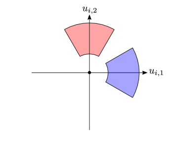
(a) Original non-convex disjoint input sets defined by (LABEL:eq:ocp_c)-(LABEL:eq:ocp_f).

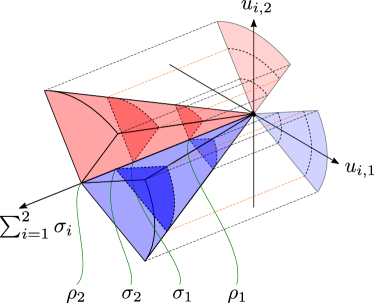
(b) The non-convexity is removed by relaxing (LABEL:eq:ocp_c) to (LABEL:eq:rcp_c)-(LABEL:eq:rcp_d).

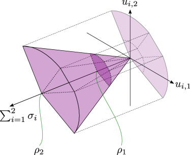
(c) The mutual exclusivity is removed by relaxing (LABEL:eq:ocp_d) to (LABEL:eq:rcp_e).

Figure 1: Problem 3.2 convexifies the input set of Problem 2.1, here shown for $M=2$, $K=1$ and $m=2$. The relaxation consists of three steps: 1(a)) (LABEL:eq:ocp_c)-(LABEL:eq:ocp_f) originally constrain each input to non-convex disjoint sets; 1(b)) by relaxing (LABEL:eq:ocp_c) to (LABEL:eq:rcp_c)-(LABEL:eq:rcp_d), individual input sets are convexified to 3D slices; 1(c)) by relaxing (LABEL:eq:ocp_d) to (LABEL:eq:rcp_e), a convex hull is obtained.

This section presents Theorem 3.3, which is the main result of the paper and states that Problem 2.1 can be solved via convex optimization under certain conditions.

Problem 2.1 is non-convex due to the input norm lower-bound in (LABEL:eq:ocp_c) and is mixed-integer due to (LABEL:eq:ocp_d). Figure 1(a) illustrates the non-convex mixed-integer nature of the problem due to the input sets being non-convex and disjoint. Consider the following convex relaxation of Problem 2.1:

Problem 3.2 ($\mathcal{R}$).

#˙x(t) = Ax(t)+B∑i=1Mui(t)+w, x(0) = x0, # γi(t)ρ1 ≤σi(t)≤γi(t)ρ2 i=1,…,M, # ∥ui(t)∥2≤σi(t) i=1,…,M, # 0≤γi(t)≤1 i=1,…,M, # ∑i=1Mγi(t) ≤K, # Ciui(t)≤0 i=1,…,M, # b(tf,x(tf)) = 0.

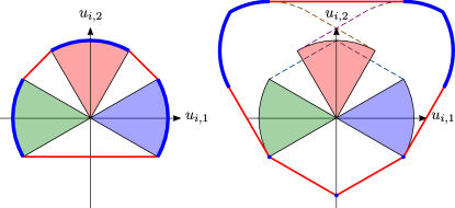
Figure 2: The relaxed input set of Problem 3.2 is the convex hull of the Minkowski sums for every combination of $K$ or fewer of the individual input sets (each one relaxed via (LABEL:eq:rcp_c)-(LABEL:eq:rcp_e)). For $M=3$, $K=2$ and $m=2$, (left) shows the case of one- and (right) shows the case of two-input set combinations, with the relaxed set shown in bold red and the boundaries of the constituent Minkowski sums shown as dashed lines. The optimal solution takes values from the extreme points, shown as blue segments. The origin is also an extreme point, corresponding to a combination of zero input sets (not shown).

By replacing (LABEL:eq:ocp_c)-(LABEL:eq:ocp_d) with (LABEL:eq:rcp_c)-(LABEL:eq:rcp_e), the input set of Problem 3.2 becomes the convex hull of the Minkowski sums of every combination of at most $K$ of the relaxed individual input sets of Problem 2.1. Figure 1 illustrates the convex relaxation for $M=2$ and $K=1$, where it is possible to also visualize the $\sigma_{i}$ slack variables to elucidate the convex lifting. Figure 2 shows the case of $M=3$ and $K=2$, where the input set is projected onto the $u_{i}$ space. It will be shown in Section 5 that the optimal solution is extremal, hence it will take values among the extreme points of the input set of Problem 3.2 with at most $K$ inputs active.

Consider the following conditions, which are sufficient to eliminate degenerate optimal solutions of Problem 3.2 that may be infeasible for Problem 2.1. To state the conditions, define an adjoint system whose output $y(t)\in\mathbb{R}^{m}$ is called the primer vector:

$$\dot{\lambda}(t)=-A^{\scriptscriptstyle\mathsf{T}}\lambda(t),\quad y(t)=B^{\scriptscriptstyle\mathsf{T}}\lambda(t). \mathcal{R}$$ (.c)

Furthermore, it will be seen in the proof of Lemma 5.6 that we are interested in “how much” $y(t)$ projects onto the $i$-th input pointing set. This is given by the following input gain measure:

$$\Gamma_{i}(t)\triangleq\mathcal{P}_{\mathcal{U}_{i}}(y(t)). \mathcal{R}$$ (.d)

Condition 1.

The adjoint system ($\mathcal{R}$.c) is observable.

Condition 2.

The adjoint system ($\mathcal{R}$.c) and pointing cone geometry (LABEL:eq:ocp_f) satisfy either:

1. $\Gamma_{i}(t)\neq 0~{}\text{a.e. }[0,t_{f}]$ $\forall i$ s.t. $y(t)\notin\mathrm{int}(\mathcal{N}_{\mathcal{U}_{i}}(0))$;

2. on any interval where $\Gamma_{i}(t)=0$, $\Gamma_{j}(t)>0$ for at least $K$ other inputs.

Condition 3.

The adjoint system ($\mathcal{R}$.c) and pointing cone geometry (LABEL:eq:ocp_f) satisfy either:

1. $\Gamma_{i}(t)\neq\Gamma_{j}(t)~{}\text{a.e. }[0,t_{f}]$ $\forall i$ s.t. $y(t)\notin\mathrm{int}(\mathcal{N}_{\mathcal{U}_{i}}(0))$;

2. on any interval where $\Gamma_{i}(t)=\Gamma_{j}(t)$, there exist $K$ inputs with $\Gamma_{k}(t)>\Gamma_{i}(t)$ or $M-K$ inputs where $\Gamma_{k}(t)<\Gamma_{i}(t)$.

Condition 4.

The following intersection holds:

$$\operatorname{range}\begin{bmatrix}\nabla_{x}b[t_{f}]^{\scriptscriptstyle\mathsf{T}}\\ \nabla_{t}b[t_{f}]^{\scriptscriptstyle\mathsf{T}}\end{bmatrix}\cap\operatorname{cone}\begin{bmatrix}\nabla_{x}m[t_{f}]^{\scriptscriptstyle\mathsf{T}}\\ \nabla_{t}m[t_{f}]\end{bmatrix}=\{0\}. \mathcal{R}$$ (.e)

We now state the main result of this paper, which claims that Problem 3.2 solves Problem 2.1 under the above conditions. The theorem is proved in Section 5.

Theorem 3.3.

The solution of Problem 3.2 is globally optimal $\text{a.e. }[0,t_{f}]$ for Problem 2.1 if Conditions 1-4 hold.

3.1 Discussion of Conditions 1-4 and Special Cases

(a) General Condition 4 requirement.

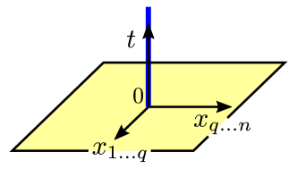
(b) Minimum-time.

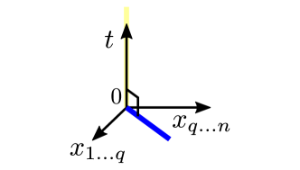
(c) Minimum-error.

Figure 3: Condition 4 for the general and two special cases.

This section describes situations when Conditions 1-4 are easy to verify. First, Condition 1 is readily verified by checking if the pair $\{-A^{\scriptscriptstyle\mathsf{T}},B^{\scriptscriptstyle\mathsf{T}}\}$ in ($\mathcal{R}$.c) is observable [25].

Condition 4 originates from the maximum principle transversality requirement ($\mathcal{G}$.l). Figure 3(a) illustrates the general requirement. As shown in Figure 3(b), the condition is satisfied for a minimum-time problem with a fixed or (partially) free terminal state. As shown in Figure 3(c), the condition is also satisfied for a fixed- or free-time problem with a (partially) penalized terminal state. Note that Assumption 2 must hold.

Conditions 2 and 3 are illustrated in Figure 4. Both conditions can be checked via matrix algebra in the special case of ray cones $\mathcal{U}_{i}=\operatorname{cone}n_{i}$ for some direction $n_{i}\in\mathbb{R}^{m}$. In this case, $\mathrm{bdry}\left(\mathcal{N}_{\mathcal{U}_{i}}(0)\right)=\{u\in\mathbb{R}^{m}:n_{i}^{\scriptscriptstyle\mathsf{T}}u=0\}$ which is a hyperplane. Consider the adjoint system ($\mathcal{R}$.c) with the “projected” primer vector:

$$n_{i}^{\scriptscriptstyle\mathsf{T}}y(t)=(Bn_{i})^{\scriptscriptstyle\mathsf{T}}\lambda(t). \mathcal{R}$$ (.f)

If the pair $\{-A^{\scriptscriptstyle\mathsf{T}},(Bn_{i})^{\scriptscriptstyle\mathsf{T}}\}$ is observable then Condition 2 case (a) holds. If not, let $\mathcal{V}_{i}$ be the unobservable subspace and consider the special case $\operatorname{range}B^{\scriptscriptstyle\mathsf{T}}(-A^{\scriptscriptstyle\mathsf{T}})^{k}\mathcal{V}_{i}\subseteq\operatorname{range}z_{i}$ $\forall k=0,\dots,n-1$ for some $z_{i}\in^{m}$. If $\mathcal{P}_{\mathcal{U}_{k}}(z_{i})>0$ and $\mathcal{P}_{\mathcal{U}_{k}}(-z_{i})>0$ for $K$ or more input pointing sets, then Condition 2 case (b) holds. Similarly, for Condition 3 we consider the projected primer vector:

$$(n_{i}-n_{j})^{\scriptscriptstyle\mathsf{T}}y(t)=\big{(}B(n_{i}-n_{j})\big{)}^{\scriptscriptstyle\mathsf{T}}\lambda(t). \mathcal{R}$$ (.g)

If the pair $\{-A^{\scriptscriptstyle\mathsf{T}},\big{(}B(n_{i}-n_{j})\big{)}^{\scriptscriptstyle\mathsf{T}}\}$ is observable then Condition 3 case (a) holds. If not, let $z_{i}\in\mathbb{R}^{m}$ be defined as before with $\mathcal{V}_{i}$ the unobservable subspace for this new system. If $\mathcal{P}_{\mathcal{U}_{k}}(z_{i})>\mathcal{P}_{\mathcal{U}_{i}}(z_{i})$ for $K$ other inputs or $\mathcal{P}_{\mathcal{U}_{k}}(z_{i})<\mathcal{P}_{\mathcal{U}_{i}}(z_{i})$ for $M-K$ other inputs, then Condition 3 case (b) holds.

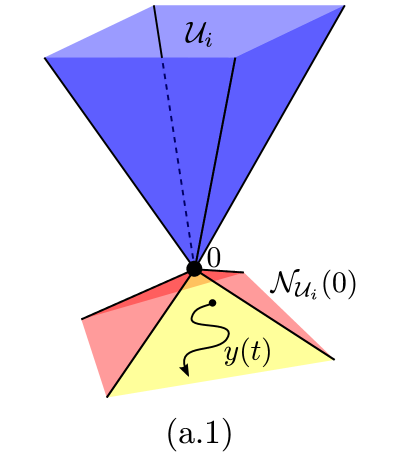
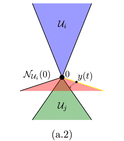
(a) When case (a) of Condition 2 fails, $y(t)$ can evolve on the normal cone boundary (a.1). Case (b) then holds if $y(t)\in\mathrm{bdry}\left(\mathcal{N}_{\mathcal{U}_{i}}(0)\right)$ projects positively onto at least $K$ other input pointing sets. For $K=1$, (a.2) illustrates a case where $y(t)$ projects positively onto $\mathcal{U}_{j}$.

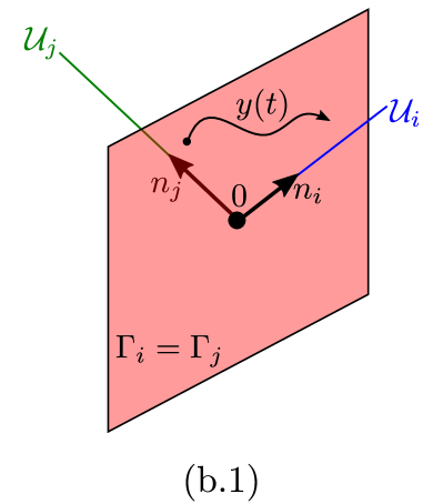
(b) When case (a) of Condition 3 fails, $y(t)$ can evolve on the manifold $\Gamma_{i}(t)=\Gamma_{j}(t)$ as shown in (b.1) for ray cones. Case (b) then holds if, for example, $y(t)$ projects more positively onto $K$ other cones. For $K=1$, (b.2) shows a situation where $y(t)$ projects more positively onto $\mathcal{U}_{k}$.

Figure 4: Visualization of Conditions 2 and 3 when their case (a) fails. In such circumstances, the conditions can nevertheless hold given the right input pointing set geometry.

4 Nonsmooth Maximum Principle

This section states a nonsmooth version of the maximum principle that we shall use for proving Theorem 3.3. Consider the following general optimal control problem:

Problem 4.4 ($\mathcal{G}$).

#˙x(t) = f(t,x(t),u(t)), x(0)=x_0, # g(t,u(t))≤0, # b(t_f,x(t_f)) = 0.

where the state trajectory $x(\cdot)$ is absolutely continuous and the control trajectory $u(\cdot)$ is measurable. The dynamics $f:\mathbb{R}\times\mathbb{R}^{n}\times\mathbb{R}^{m}\to\mathbb{R}^{n}$ are convex and continuously differentiable. The terminal cost $m:\mathbb{R}\times\mathbb{R}^{n}\to\mathbb{R}$, the input constraint $g:\mathbb{R}\times\mathbb{R}^{m}\to\mathbb{R}^{n_{g}}$, and the terminal constraint $b:\mathbb{R}\times\mathbb{R}^{n}\to\mathbb{R}^{n_{b}}$ are convex. Let us denote the terminal manifold as $\mathcal{T}\triangleq\{x\in\mathbb{R}^{n}:\textnormal{\eqref{eq:ocp_general_d} holds}\}$. The Hamiltonian function is defined as:

$$H(t,x(t),u(t),\lambda(t))\triangleq\lambda(t)^{\scriptscriptstyle\mathsf{T}}f[t], \mathcal{G}$$ (.h)

where $\lambda(\cdot)$ is the adjoint variable trajectory. We now state the nonsmooth maximum principle, due to [26, Theorem 8.7.1] (see also [27, 28]), which specifies the necessary conditions of optimality for Problem 4.4.

Theorem 4.5.

[Maximum Principle] Let $x(\cdot)$ and $u(\cdot)$ be optimal on the interval $[0,t_{f}]$. There exist an abnormal multiplier $\alpha\leq 0$ and an absolutely continuous $\lambda(\cdot)$ such that the following conditions are satisfied:

1. Non-triviality:

   $$(\alpha,\lambda(t))\neq 0~{}\forall t\in[0,t_{f}]; \mathcal{G}$$ (.i)

2. Pointwise maximum:

   $$u(t)=\operatorname*{argmax}_{v\in\textnormal{\eqref{eq:ocp_general_c}}}H(t,x(t),v,\lambda(t))~{}\text{a.e. }[0,t_{f}]; \mathcal{G}$$ (.j)

3. The differential equations:

   $$\dot{x}(t)=\nabla_{\lambda}H[t]^{\scriptscriptstyle\mathsf{T}}~{}\text{a.e. }[0,t_{f}], \mathcal{G}$$ (.ka)

   $$\dot{\lambda}(t)=-\nabla_{x}H[t]^{\scriptscriptstyle\mathsf{T}}~{}\text{a.e. }[0,t_{f}], \mathcal{G}$$ (.kb)

   $$\dot{H}[t]=\nabla_{t}H[t]~{}\text{a.e. }[0,t_{f}]; \mathcal{G}$$ (.kc)

4. Transversality:

   $$\lambda(t_{f})\in\alpha\partial_{x}m[t_{f}]^{\scriptscriptstyle\mathsf{T}}+\mathcal{N}_{\mathcal{T}}(x(t_{f})), \mathcal{G}$$ (.la)

   $$0\in H[t_{f}]+\alpha\partial_{t}m[t_{f}]+\mathcal{N}_{\mathcal{T}}(t_{f}). \mathcal{G}$$ (.lb)

5 Lossless Convexification Proof

This section proves Theorem 3.3 in two steps. First, the output of Problem 3.2 is shown to be feasible for Problem 2.1 via a maximum principle argument. Second, this solution is shown to also be globally optimal via an equal cost function argument.

Lemma 5.6.

The solution of Problem 3.2 is feasible $\text{a.e. }[0,t_{f}]$ for Problem 2.1 if Conditions 1-4 hold.

Proof. The proof uses the maximum principle from Theorem 4.5. For Problem 3.2, the adjoint and Hamiltonian dynamics follow from ($\mathcal{G}$.kb) and ($\mathcal{G}$.kc):

$$\dot{\lambda}(t)=-A^{\scriptscriptstyle\mathsf{T}}\lambda(t)~{}\text{a.e. }[0,t_{f}], \mathcal{G}$$ (.ma)

$$\dot{H}[t]=0~{}\text{a.e. }[0,t_{f}], \mathcal{G}$$ (.mb)

Using the subdifferential basic chain rule [29, Theorem 10.6], the transversality condition ($\mathcal{G}$.l) yields:

$$\lambda(t_{f})=\nabla_{x}m[t_{f}]^{\scriptscriptstyle\mathsf{T}}\alpha+\nabla_{x}b[t_{f}]^{\scriptscriptstyle\mathsf{T}}\beta, \mathcal{G}$$ (.na)

$$H[t_{f}]=-\nabla_{t}m[t_{f}]\alpha-\nabla_{t}b[t_{f}]^{\scriptscriptstyle\mathsf{T}}\beta, \mathcal{G}$$ (.nb)

for some $\beta\in\mathbb{R}^{n_{b}}$. Due to ($\mathcal{G}$.mb), ($\mathcal{G}$.nb) and absolute continuity, we have [30, Theorem 9]:

$$H[t]=-\nabla_{t}m[t_{f}]\alpha-\nabla_{t}b[t_{f}]^{\scriptscriptstyle\mathsf{T}}\beta,~{}\forall t\in[0,t_{f}]. \mathcal{G}$$ (.o)

We claim that the primer vector $y(t)\neq 0~{}\text{a.e. }[0,t_{f}]$. Since $y(t)$ is the output of ($\mathcal{R}$.c), it is an analytic function and $y(t)=0$ either $\forall t\in[0,t_{f}]$ or at a countable number of instances [5, 7]. By contradiction, suppose that $y(t)=0$ $\forall t\in[0,t_{f}]$. Since Condition 1 holds, $\lambda(0)=0$. Since ($\mathcal{G}$.ma) is homogeneous, $\lambda(t)=0$ $\forall t\in[0,t_{f}]$. The transversality condition ($\mathcal{G}$.n) hence simplifies to:

$$\begin{bmatrix}\nabla_{x}m[t_{f}]^{\scriptscriptstyle\mathsf{T}}\\ \nabla_{t}m[t_{f}]\end{bmatrix}(-\alpha)=\begin{bmatrix}\nabla_{x}b[t_{f}]^{\scriptscriptstyle\mathsf{T}}\\ \nabla_{t}b[t_{f}]^{\scriptscriptstyle\mathsf{T}}\end{bmatrix}\beta, \mathcal{G}$$ (.p)

and since Condition 4 holds, $\alpha=0$. Hence $(\alpha,\lambda(t))=0$ $\forall t\in[0,t_{f}]$, which violates non-triviality ($\mathcal{G}$.i). Therefore it must be that $y(t)\neq 0~{}\text{a.e. }[0,t_{f}]$. Because the necessary conditions are scale-invariant, we can set $\alpha=-1$ without loss of generality. The pointwise maximum condition ($\mathcal{G}$.j) implies that the following must hold $\text{a.e. }[0,t_{f}]$: #constraints (LABEL:eq:rcp_c)-(LABEL:eq:rcp_g) hold.

We shall now analyze the optimality conditions of ($\mathcal{G}$.q). For concise notation, the time argument $t$ shall be omitted. Expressing ($\mathcal{G}$.q) as a minimization and treating constraints (LABEL:eq:rcp_e) and (LABEL:eq:rcp_f) implicitly, we can write the Lagrangian of ($\mathcal{G}$.q) [31]:

$$\mathcal{L}(u_{i},\gamma_{i},\sigma_{i},\lambda_{1\dots 4}^{i})=\textstyle\sum_{i=1}^{M}-y^{\scriptscriptstyle\mathsf{T}}u_{i}+\lambda_{1}^{i}(\|u_{i}\|_{2}- \mathcal{G}$$ (.qr)

$$\hskip 28.45274pt\sigma_{i})+\lambda_{2}^{i}(\gamma_{i}\rho_{1}-\sigma_{i})+\lambda_{3}^{i}(\sigma_{i}-\gamma_{i}\rho_{2})+{\lambda_{4}^{i}}^{\scriptscriptstyle\mathsf{T}}C_{i}u_{i},$$

where $\lambda_{j}^{i}\geq 0$ are Lagrange multipliers satisfying the following complementarity conditions:

$$\lambda_{1}^{i}(\|u_{i}\|_{2}-\sigma_{i})=0, \mathcal{G}$$ (.qsa)

$$\lambda_{2}^{i}(\gamma_{i}\rho_{1}-\sigma_{i})=0, \mathcal{G}$$ (.qsb)

$$\lambda_{3}^{i}(\sigma_{i}-\gamma_{i}\rho_{2})=0, \mathcal{G}$$ (.qsc)

$$\lambda_{4}^{i}\circ C_{i}u_{i}=0. \mathcal{G}$$ (.qsd)

Next, the Lagrange dual function is given by:

$$g(\lambda_{1\dots 4}^{i})=\inf_{u_{i},\gamma_{i},\sigma_{i}}\mathcal{L}(u_{i},\gamma_{i},\sigma_{i},\lambda_{1\dots 4}^{i})$$

$$\phantom{g(\lambda_{1\dots 4}^{i})}=\textstyle\sum_{i=1}^{M}\inf_{\sigma_{i}}\left[(\lambda_{3}^{i}-\lambda_{2}^{i}-\lambda_{1}^{i})\sigma_{i}\right]-$$

$$\phantom{g(\lambda_{1\dots 4}^{i})=}\textstyle\sum_{i=1}^{M}\sup_{u_{i}}\left[(y-C_{i}^{\scriptscriptstyle\mathsf{T}}\lambda_{4}^{i})^{\scriptscriptstyle\mathsf{T}}u_{i}-\lambda_{1}^{i}\|u_{i}\|_{2}\right]+$$

$$\phantom{g(\lambda_{1\dots 4}^{i})=}\textstyle\inf_{\textnormal{\eqref{eq:rcp_e},\eqref{eq:rcp_f}}}\textstyle\sum_{i=1}^{M}(\lambda_{2}^{i}\rho_{1}-\lambda_{3}^{i}\rho_{2})\gamma_{i}. \mathcal{G}$$ (.qt)

The dual function bounds the primal optimal cost from above. A non-trivial upper-bound requires:

$$\|y-C_{i}^{\scriptscriptstyle\mathsf{T}}\lambda_{4}^{i}\|_{2}\leq\lambda_{1}^{i}, \mathcal{G}$$ (.qua)

$$\lambda_{3}^{i}-\lambda_{2}^{i}-\lambda_{1}^{i}=0, \mathcal{G}$$ (.qub)

where the first inequality is akin to the $\|\cdot\|_{2}$ conjugate function [31, Example 3.26]. However, note that if ($\mathcal{G}$.qua) is strict then $\|u_{i}\|_{2}=0$ is optimal, which is trivially feasible for Problem 2.1. Substituting ($\mathcal{G}$.qub) into ($\mathcal{G}$.qua) gives the following condition for non-trivial solutions:

$$\|y-C_{i}^{\scriptscriptstyle\mathsf{T}}\lambda_{4}^{i}\|_{2}=\lambda_{3}^{i}-\lambda_{2}^{i}. \mathcal{G}$$ (.qv)

Next, note that a non-trivial solution implies $\gamma_{i}>0$. Due to Assumption 3, ($\mathcal{G}$.qsb) and ($\mathcal{G}$.qsc), a non-trivial solution cannot have $\lambda_{2}^{i}>0$ and $\lambda_{3}^{i}>0$ simultaneously. Furthemore, ($\mathcal{G}$.qt) reveals that $\gamma_{i}>0$ is not sub-optimal if and only if $\lambda_{2}^{i}\rho_{1}-\lambda_{3}^{i}\rho_{2}\leq 0$. Hence $\lambda_{2}^{i}=0$ and $\lambda_{3}^{i}\geq 0$ are necessary for optimality. As a result ($\mathcal{G}$.qv) simplifies to:

$$\|y-C_{i}^{\scriptscriptstyle\mathsf{T}}\lambda_{4}^{i}\|_{2}=\lambda_{3}^{i}. \mathcal{G}$$ (.qw)

Next, note that at optimality the left-hand side of ($\mathcal{G}$.qw) equals the Eucledian projection onto $\mathcal{U}_{i}$, i.e. $\|y-C_{i}^{\scriptscriptstyle\mathsf{T}}\lambda_{4}^{i}\|_{2}=\mathcal{P}_{\mathcal{U}_{i}}(y)$. This can be shown by contradiction using Assumption 2, ($\mathcal{G}$.qsd) and that it is optimal to choose $u_{i}=\|u_{i}\|_{2}(y-C_{i}^{\scriptscriptstyle\mathsf{T}}\lambda_{4}^{i})/\|y-C_{i}^{\scriptscriptstyle\mathsf{T}}\lambda_{4}^{i}\|_{2}$ in ($\mathcal{G}$.qt). Note that the degenerate case of $u_{i}\neq 0$ and $\|y-C_{i}^{\scriptscriptstyle\mathsf{T}}\lambda_{4}^{i}\|_{2}=0$ is eliminated by Condition 2, as discussed below. Thus ($\mathcal{G}$.qw) simplifies to the following relationship, which we call the characteristic equation of non-trivial solutions to ($\mathcal{G}$.q):

$$\mathcal{P}_{\mathcal{U}_{i}}(y)=\lambda_{3}^{i}. \mathcal{G}$$ (.qx)

Note that when $\lambda_{3}^{i}>0$ then $\|u_{i}\|_{2}=\sigma_{i}=\gamma_{i}\rho_{2}$ due to ($\mathcal{G}$.qsc) and ($\mathcal{G}$.qub). Substituting ($\mathcal{G}$.qx) into ($\mathcal{G}$.qt) yields:

$$g(\lambda_{1\dots 4}^{i})=-\rho_{2}\textstyle\sup_{\textnormal{\eqref{eq:rcp_e},\eqref{eq:rcp_f}}}\textstyle\sum_{i=1}^{K^{\prime}}\mathcal{P}_{\mathcal{U}_{i}}(y)\gamma_{i}, \mathcal{G}$$ (.qy)

where we assume that the characteristic equation ($\mathcal{G}$.qx) does not hold for $i=K^{\prime}+1,\dots,M$ such that $\gamma_{i>K^{\prime}}=0$. To facilitate discussion, define the $i$-th input gain as in ($\mathcal{R}$.d). Note that $\Gamma_{i}\geq 0$ due to ($\mathcal{G}$.qx). Thus ($\mathcal{G}$.qy) becomes:

$$g(\lambda_{1\dots 4}^{i})=-\rho_{2}\textstyle\sup_{\textnormal{\eqref{eq:rcp_e},\eqref{eq:rcp_f}}}\textstyle\sum_{i=1}^{K^{\prime}}\Gamma_{i}\gamma_{i}. \mathcal{G}$$ (.qz)

Without loss of generality, assume a descending ordering $\Gamma_{i}\geq\Gamma_{j}$ for $i>j$. Let $K^{\prime\prime}\triangleq\min\{K,K^{\prime}\}$. By inspection of ($\mathcal{G}$.qz), the condition:

$$\Gamma_{K^{\prime\prime}}>0~{}\land~{}\Gamma_{K^{\prime\prime}}>\Gamma_{K^{\prime\prime}+1}, \mathcal{G}$$ (.qaa)

is sufficient to ensure that it is optimal to set

$$\gamma_{i}=\begin{cases}1&\text{for }i\leq K^{\prime\prime},\\ 0&\text{otherwise.}\end{cases} \mathcal{G}$$ (.qab)

The lemma is proved if ($\mathcal{G}$.qaa) holds $\text{a.e. }[0,t_{f}]$. However, this holds by assumption due to Conditions 2 and 3. In particular, Condition 2 case (a) assures that $\Gamma_{K^{\prime\prime}}>0~{}\text{a.e. }[0,t_{f}]$. If on some interval $\Gamma_{k}=0$, Condition 2 case (b) assures that $k>K^{\prime\prime}$. Next, if $K^{\prime\prime}<K$ then due to $\Gamma_{K^{\prime\prime}}>0$ and the definition of $K^{\prime}$, it must be that $\Gamma_{K^{\prime\prime}+1}=0\Rightarrow\Gamma_{K^{\prime\prime}}>\Gamma_{K^{\prime\prime}+1}$. On the other hand, if $K^{\prime\prime}=K$ then Condition 3 case (a) assures that $\Gamma_{K}>\Gamma_{K+1}~{}\text{a.e. }[0,t_{f}]$. If on some interval $\Gamma_{k}=\Gamma_{k+1}$, Condition 3 case (b) assures that $k\neq K$.

Thus, ($\mathcal{G}$.qaa) holds $\text{a.e. }[0,t_{f}]$ and the lemma is proved. From ($\mathcal{G}$.qab), the structure of the optimal solution is bang-bang with at most $K$ inputs active $\text{a.e. }[0,t_{f}]$. ∎

Lemma 5.6 guarantees that solving Problem 3.2 yields a feasible solution of Problem 2.1. We will now show that this solution is globally optimal, thus proving Theorem 3.3.

Proof of Theorem 3.3. The solution of Problem 3.2 is feasible $\text{a.e. }[0,t_{f}]$ for Problem 2.1 due to Lemma 5.6. Furthermore, the cost functions of Problems 2.1 and 3.2 are the same. The optimal costs thus satisfy $J_{\mathcal{O}}^{*}\leq J_{\mathcal{R}}^{*}$. However, any solution of Problem 2.1 is feasible for Problem 3.2 by setting $\sigma_{i}(t)=\|u_{i}(t)\|_{2}$, thus $J_{\mathcal{R}}^{*}\leq J_{\mathcal{O}}^{*}$. Therefore $J_{\mathcal{R}}^{*}=J_{\mathcal{O}}^{*}$ so the solution of Problem 3.2 is globally optimal for Problem 2.1 $\text{a.e. }[0,t_{f}]$. ∎

Theorem 3.3 implies that Problem 2.1 is solved in polynomial time by an SOCP solver applied to Problem 3.2. This can be done efficiently with several numerically reliable SOCP solvers [32]. This demonstrates that the class of $\mathcal{NP}$-hard optimal control problems defined by Problem 2.1 under Conditions 1-4 is in fact of $\mathcal{P}$ complexity.

6 Numerical Example

This section shows how a trajectory for spacecraft docking to a rotating space station can be computed more efficiently via Problem 3.2 versus a standard MICP approach. Python source code for this example is available online. Figure 5 illustrates the scenario. The spacecraft’s dynamics are described in the rotating frame by:

$$\dot{x}(t)=A(\omega)x(t)+B\textstyle\sum_{i=1}^{M}u_{i}(t), \mathcal{G}$$ (.qac)

where $x(t)=(r(t),v(t)):\mathbb{R}_{+}\to\mathbb{R}^{6}$ is the position and velocity state, $\omega\in\mathbb{R}^{3}$ is the space station’s constant angular velocity vector, and

$$A(\omega)\triangleq\begin{bmatrix}0&I\\ -S(\omega)^{2}&-2S(\omega)\end{bmatrix},~{}B\triangleq\begin{bmatrix}0\\ I\end{bmatrix}, \mathcal{G}$$ (.qad)

where $S(\omega)\in\mathbb{R}^{3\times 3}$ is the skew-symmetric matrix representation of the cross product $\omega\times(\cdot)$.

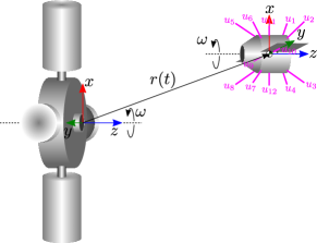
Figure 5: Spacecraft docking to a rotating space station is modelled in the space station’s rotating frame. The spacecraft is assumed to have matched the space station angular velocity.

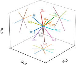
Figure 6: The spacecraft’s reaction control system is capable of producing up to $K=4$ out of $M=12$ acceleration vectors, acting through the center of mass.

We assume that the spacecraft is equipped with a reaction control system capable of producing up to $K=4$ acceleration vectors from a total of $M=12$ distinct directions, as illustrated in Figure 6. Acceleration vectors along the positive $z$-axis point with a pitch and roll of $40$ degrees. Along the negative $z$-axis, the pitch and roll is $30$ degrees. The docking port is positioned at the origin and rotates with the space station. The spacecraft is assumed to rotate with the same angular velocity $\omega$ and is tasked to perform translation control to berth with the docking port. We use the parameters:

$$\omega=(0,0,1)~{}\text{rpm},~{}\rho_{1}=1~{}$\mathrm{mm}\text{\,}{\mathrm{s}}^{-2}$,~{}\rho_{2}=10~{}$\mathrm{mm}\text{\,}{\mathrm{s}}^{-2}$,$$

$$m[t_{f}]=t_{f},~{}r(0)=(5,5,100)~{}$\mathrm{m}$,~{}v(0)=(0,0,0)~{}$\mathrm{m}\text{\,}{\mathrm{s}}^{-1}$,$$

$$r(t_{f})=(0,0,0)~{}$\mathrm{m}$,~{}v(t_{f})=(0,0,-0.01)~{}$\mathrm{m}\text{\,}{\mathrm{s}}^{-1}$,$$

where the initial velocity choice makes the spacecraft’s inertial velocity $\omega\times r(0)$ $\mathrm{m}\text{\,}{\mathrm{s}}^{-1}$. A more realistic setting would be $v(0)=-\omega\times r(0)$ which makes the inertial velocity zero. The motivation for the present choice is to enrich the solution. Since the cost is linear in $t_{f}$, both bisection and golden search can be applied to find the minimum $t_{f}$ [6, 33].

Conditions 1-4 are satisfied by this problem. Condition 1 is satisfied since $\{-A(\omega)^{\scriptscriptstyle\mathsf{T}},B^{\scriptscriptstyle\mathsf{T}}\}$ is observable. Condition 4 is satisfied according to the minimum-time special case in Figure 3(b). Conditions 2 and 3 hold following the discussion in Section 3.1 and noting that the primer vector $y(\cdot)$ in ($\mathcal{R}$.c) can only be persistently normal to $\omega$ or to vectors normal to $\omega$. The conditions are checked automatically via a script in the public source code.

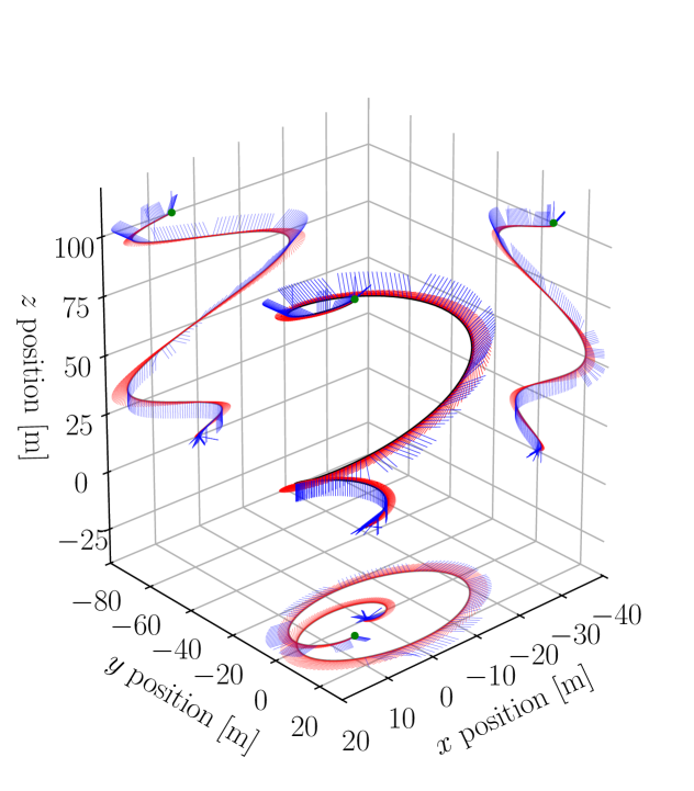
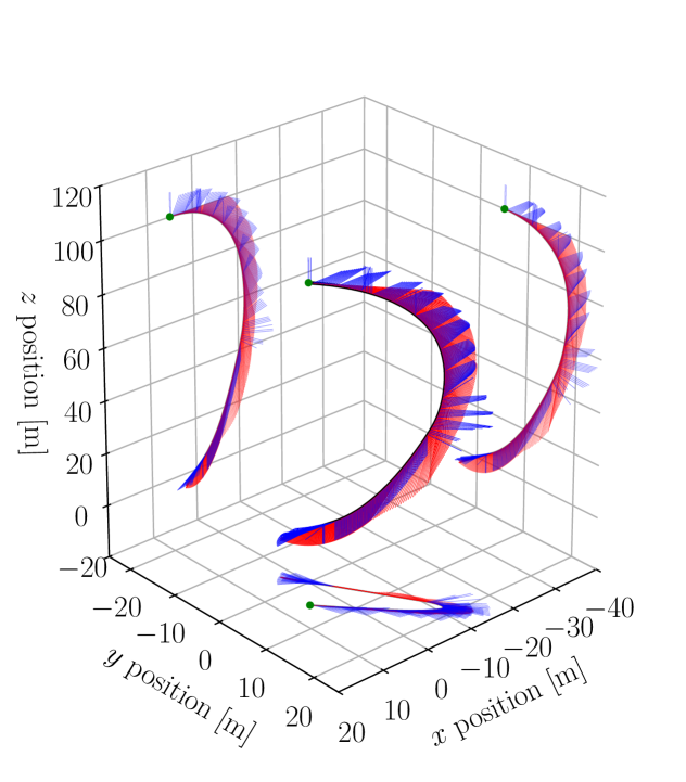
(a) Trajectory in the space station rotating frame (top), and the inertial frame (bottom). Time of flight $t_{f}=135~{}$\mathrm{s}$$.

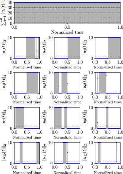
(b) Optimal input norm history in $\mathrm{mm}\text{\,}{\mathrm{s}}^{-2}$. The bang-bang nature of the solution is clearly visible. Blue markers show $\sigma_{i}(t)$.

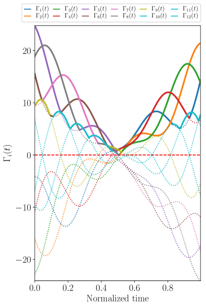
(c) Time history of the input gain ($\mathcal{R}$.d). Bold lines show when the corresponding input is active.

Figure 7: Optimal docking trajectory (7(a)) together with the input (7(b)) and dual variable (7(c)) histories. In (7(a)), red vectors show the scaled velocity, blue vectors show the scaled thrust (negative of acceleration), and the green marker shows the initial position.

The dynamics ($\mathcal{G}$.qac) are discretized using zeroth-order hold over a uniform temporal grid of 300 nodes. Python 2.7.15 with ECOS 2.0.7.post1 [34] is used for implementation on a Ubuntu 18.04.1 64-bit platform with a 2.5 GHz Intel Core i5-7200U CPU and 8 GB of RAM. The solution and runtime are compared to a mixed-integer formulation where (LABEL:eq:ocp_d) is implemented directly as a binary constraint using Gurobi 8.1 [35].

Figure 7 shows the resulting state, input and input gain trajectories for the globally optimal solution. The solution is obtained in $20~{}$\mathrm{s}$$ via Problem 3.2, whereas MICP takes an intractable $6200~{}$\mathrm{s}$$. This is expected, since solving Problem 3.2 relies on an SOCP solver with polynomial time complexity, whereas MICP has exponential time complexity.

Figure 7(b) confirms that the constraints (LABEL:eq:ocp_c)-(LABEL:eq:ocp_e) are satisfied. In particular, the thrust magnitude is bang-bang as predicted in Lemma 5.6. The intermediate thrusts occuring at rising and falling edges are discretization artifacts since the lossless convexification guarantee is only “almost everywhere” in nature. These artifacts have been observed since the early days of the lossless convexification method [4]. Figure 7(c) confirms the optimal input structure ($\mathcal{G}$.qab). In particular, for the minimum-time solution it is always the inputs corresponding to the largest $K=4$ gain values $\Gamma_{i}(t)$ that are active.

7 Future Work

The primary focus of future work is to expand the class of problems that can be handled. This includes using different norm types and bounds in (LABEL:eq:ocp_c), adding a lower-bound constraint to (LABEL:eq:ocp_e) (i.e. minimum number of active inputs), relaxing Assumption 1 to non-overlapping input pointing sets, considering linear time-varying dynamics in (LABEL:eq:ocp_b), and introducing state constraints. A minor caveat of the Lemma 5.6 proof is that conditions which are proven to hold “almost everywhere” are assumed not to fail on nowhere dense sets of positive measure (e.g. the fat Cantor set) [36]. We do not expect this pathology to occur for any practical problem, and in the future we seek to rigorously eliminate this pathology.

8 Conclusion

This paper presented a lossless convexification method for solving a class of optimal control problems with semi-continuous input norms. Such problems are inherently mixed-integer in nature. By relaxing the problem to a convex one and proving that the relaxed solution is globally optimal for the original problem, solutions can be found via convex optimization in polynomial time. Our result thus shows that a practical class of $\mathcal{NP}$-hard optimal control problems is in fact of $\mathcal{P}$ complexity. The algorithm is amenable to real-time onboard implementation and can be used to accelerate design trade studies.

9 Acknowledgements

We thank Emma Hansen for conducting preliminary simulations.

References

- [1] MOSEK ApS, MOSEK Modeling Cookbook, 3.1 ed., July 2019.
- [2] A. Bemporad and M. Morari, “Control of systems integrating logic, dynamics, and constraints,” Automatica, vol. 35, pp. 407–427, mar 1999.
- [3] T. H. Cormen, C. E. Leiserson, R. L. Rivest, and C. Stein, Introduction to Algorithms. MIT Press, 3 ed., 2009.
- [4] B. Açıkmeşe and S. R. Ploen, “Convex programming approach to powered descent guidance for Mars landing,” Journal of Guidance, Control, and Dynamics, vol. 30, pp. 1353–1366, sep 2007.
- [5] B. Açıkmeşe and L. Blackmore, “Lossless convexification of a class of optimal control problems with non-convex control constraints,” Automatica, vol. 47, pp. 341–347, feb 2011.
- [6] L. Blackmore, B. Açıkmeşe, and D. P. Scharf, “Minimum-landing-error powered-descent guidance for Mars landing using convex optimization,” Journal of Guidance, Control, and Dynamics, vol. 33, pp. 1161–1171, jul 2010.
- [7] J. M. Carson III, B. Açıkmeşe, and L. Blackmore, “Lossless convexification of powered-descent guidance with non-convex thrust bound and pointing constraints,” in Proceedings of the 2011 American Control Conference, IEEE, jun 2011.
- [8] B. Açıkmeşe, J. M. Carson III, and L. Blackmore, “Lossless convexification of nonconvex control bound and pointing constraints of the soft landing optimal control problem,” IEEE Transactions on Control Systems Technology, vol. 21, pp. 2104–2113, nov 2013.
- [9] C. A. Pascucci, M. Szmuk, and B. Açıkmeşe, “Optimal real-time force rendering for on-orbit structures assembly,” in 10th International ESA Conference on Guidance, Navigation & Control Systems, ESA, may 2017.
- [10] M. W. Harris and B. Açıkmeşe, “Lossless convexification for a class of optimal control problems with linear state constraints,” in 52nd IEEE Conference on Decision and Control, IEEE, dec 2013.
- [11] M. W. Harris and B. Açıkmeşe, “Lossless convexification for a class of optimal control problems with quadratic state constraints,” in 2013 American Control Conference, IEEE, jun 2013.
- [12] M. W. Harris and B. Açıkmeşe, “Lossless convexification of non-convex optimal control problems for state constrained linear systems,” Automatica, vol. 50, pp. 2304–2311, sep 2014.
- [13] L. Blackmore, B. Açıkmeşe, and J. M. Carson III, “Lossless convexification of control constraints for a class of nonlinear optimal control problems,” Systems & Control Letters, vol. 61, pp. 863–870, aug 2012.
- [14] Z. Zhang, J. Wang, and J. Li, “Lossless convexification of nonconvex MINLP on the UAV path-planning problem,” Optimal Control Applications and Methods, vol. 39, pp. 845–859, dec 2017.
- [15] Y. Mao, M. Szmuk, and B. Açıkmeşe, “Successive convexification of non-convex optimal control problems and its convergence properties,” in 2016 IEEE 55th Conference on Decision and Control (CDC), IEEE, dec 2016.
- [16] Y. Mao, D. Dueri, M. Szmuk, and B. Açıkmeşe, “Successive Convexification of Non-Convex Optimal Control Problems with State Constraints,” arXiv e-prints, p. arXiv:1701.00558, Jan. 2017.
- [17] D. Dueri, Y. Mao, Z. Mian, J. Ding, and B. Açıkmeşe, “Trajectory optimization with inter-sample obstacle avoidance via successive convexification,” in 2017 IEEE 56th Annual Conference on Decision and Control (CDC), IEEE, dec 2017.
- [18] Y. Mao, M. Szmuk, and B. Açıkmeşe, “Successive Convexification: A Superlinearly Convergent Algorithm for Non-convex Optimal Control Problems,” arXiv e-prints, p. arXiv:1804.06539, Apr. 2018.
- [19] R. Bonalli, A. Cauligi, A. Bylard, and M. Pavone, “GuSTO: Guaranteed sequential trajectory optimization via sequential convex programming,” in 2019 IEEE International Conference on Robotics and Automation (ICRA), IEEE, may 2019.
- [20] M. Szmuk, B. Açıkmeşe, and A. W. Berning, “Successive convexification for fuel-optimal powered landing with aerodynamic drag and non-convex constraints,” in AIAA Guidance, Navigation, and Control Conference, American Institute of Aeronautics and Astronautics, jan 2016.
- [21] M. Szmuk, T. P. Reynolds, and B. Açıkmeşe, “Successive Convexification for Real-Time 6-DoF Powered Descent Guidance with State-Triggered Constraints,” arXiv e-prints, p. arXiv:1811.10803, Nov. 2018.
- [22] M. Szmuk, T. P. Reynolds, B. Açıkmeşe, M. Mesbahi, and J. M. Carson III, “Successive Convexification for 6-DoF Powered Descent Guidance with Compound State-Triggered Constraints,” arXiv e-prints, p. arXiv:1901.02181, Jan. 2019.
- [23] T. Reynolds, M. Szmuk, D. Malyuta, M. Mesbahi, B. Açıkmeşe, and J. M. Carson III, “A state-triggered line of sight constraint for 6-DoF powered descent guidance problems,” in AIAA Scitech 2019 Forum, American Institute of Aeronautics and Astronautics, jan 2019.
- [24] D. Malyuta, T. P. Reynolds, M. Szmuk, B. Açıkmeşe, and M. Mesbahi, “Fast trajectory optimization via successive convexification for spacecraft rendezvous with integer constraints,” in Scitech Forum (accepted), p. arXiv:1906.04857, AIAA, jan 2019.
- [25] P. Antsaklis and A. Michel, A Linear Systems Primer. Boston, MA: Birkhauser, 2007.
- [26] R. Vinter, Optimal Control. Birkhauser, 2000.
- [27] F. Clarke, “The Pontryagin maximum principle and a unified theory of dynamic optimization,” Proceedings of the Steklov Institute of Mathematics, vol. 268, pp. 58–69, Apr. 2010.
- [28] R. F. Hartl, S. P. Sethi, and R. G. Vickson, “A survey of the maximum principles for optimal control problems with state constraints,” SIAM Review, vol. 37, pp. 181–218, jun 1995.
- [29] R. T. Rockafellar and R. J. B. Wets, Variational Analysis. Springer Berlin Heidelberg, 1998.
- [30] D. E. Varberg, “On absolutely continuous functions,” The American Mathematical Monthly, vol. 72, p. 831, Oct. 1965.
- [31] S. Boyd and L. Vandenberghe, Convex Optimization. Cambridge University Press, 2004.
- [32] D. Dueri, J. Zhang, and B. Açıkmeşe, “Automated custom code generation for embedded, real-time second order cone programming,” IFAC Proceedings Volumes, vol. 47, no. 3, pp. 1605–1612, 2014.
- [33] M. J. Kochenderfer and T. A. Wheeler, Algorithms for Optimization. Cambridge, Massachusetts: The MIT Press, 2019.
- [34] A. Domahidi, E. Chu, and S. Boyd, “ECOS: An SOCP solver for embedded systems,” in 2013 European Control Conference (ECC), IEEE, jul 2013.
- [35] L. Gurobi Optimization, “Gurobi optimizer reference manual,” 2018.
- [36] J. C. Morgan II, Point Set Theory. CRC Press, 1990.