Fast Transient Simulation of High-Speed Channels Using Recurrent Neural Network

Abstract

Generating eye diagrams by using a circuit simulator can be very computationally intensive, especially in the presence of nonlinearities. It often involves multiple Newton-like iterations at every time step when a SPICE-like circuit simulator handles a nonlinear system in the transient regime. In this paper, we leverage machine learning methods, to be specific, the recurrent neural network (RNN), to generate black-box macro-models and achieve significant reduction of computation time. Through the proposed approach, an RNN model is first trained and then validated on a relatively short sequence generated from a circuit simulator. Once the training completes, the RNN can be used to make predictions on the remaining sequence in order to generate an eye diagram. The training cost can also be amortized when the trained RNN starts making predictions. Besides, the proposed approach requires no complex circuit simulations nor substantial domain knowledge. We use two high-speed link examples to demonstrate that the proposed approach provides adequate accuracy while the computation time can be dramatically reduced. In the high-speed link example with a PAM4 driver, the eye diagram generated by RNN models shows good agreement with that obtained from a commercial circuit simulator. This paper also investigates the impacts of various RNN topologies, training schemes, and tunable parameters on both the accuracy and the generalization capability of an RNN model. It is found out that the long short-term memory (LSTM) network outperforms the vanilla RNN in terms of the accuracy in predicting transient waveforms.

I Introduction

In the area of signal integrity, eye diagrams have become important metrics to assess the performance of a high-speed channel. In order to generate an eye diagram, transient waveforms are first obtained from a circuit simulator and then overlaid. Generating eye diagrams by using a circuit simulator can be very computationally intensive, especially in the presence of nonlinearities. As shown in Figure 1, there are often multiple Newton-like iterations involved at every time step when a SPICE-like circuit simulator handles a nonlinear system in the transient regime [1]. Given the size of a practical and large-scale circuit, the runtime of a circuit simulator on modern processors can be hours, days, or even weeks. There are many efforts in seeking novel numerical techniques to improve the computation efficiency of a circuit simulator. For example, people are using hardware accelerators including FPGAs [1] and GPUs [2] to achieve the acceleration of matrix factorization in a circuit simulator. There are also works in efficiently generating eye diagrams, for example, using shorter bit patterns instead of the pseudo-random bit sequence as input sources to simulate the worst-case eye diagram [3]. In this work, we propose taking a different route and using machine learning methods, to be specific, recurrent neural network (RNN), to improve the efficiency of a circuit simulator.

Figure 1: Flow chart of a circuit simulator [1].

Recently, many remarkable results are reported on modern time-series techniques by using RNN in the fields such as language modeling, machine translation, chatbot, and forecasting [4, 5, 6, 7, 8]. There are also a number of prior attempts in incorporating RNN into modeling and simulating electronic devices and systems. For example, researchers propose combining a NARX (nonlinear auto-regressive network) topology with a feedforward neural network in modeling nonlinear RF devices [9]. A variant of RNN, known as Elman RNN (ERNN), is applied in simulating digital designs [10, 11]. More recently, researchers present an ERNN-based model in simulating electrostatic discharge (ESD) [12]. The aforementioned two topologies, to be specific, NARX-RNN and ERNN, will be discussed in details in the following sections. It is also worth mentioning that machine learning methods in general have been seen into many applications related to electronic designs such as modeling high-speed channels [13, 14, 15], replacing computationally expensive full-wave electromagnetic simulations [16, 17], and building macro-model from S-parameters [18, 19].

Through the proposed approach, a modern ERNN is first trained and then validated on a relatively short sequence generated from a circuit simulator. Once the training completes, the RNN can be used to make predictions on the remaining sequence in order to generate an eye diagram. The training cost can also be amortized when the trained RNN starts making predictions. As the time-domain waveforms are generated from RNN through inference instead of iterations of solving linear systems involved in a circuit simulator, it significantly improves the computation efficiency. Besides, the proposed approach requires no complex circuit simulations nor substantial domain knowledge. We demonstrate through two examples that the proposed approach can meet the accuracy of transistor-level simulation while the run time can be dramatically reduced.

In this work, we also investigate the performance of ERNNs built with different recurrent units, to be specific, vanilla recurrent neural network (VRNN), long short-term memory (LSTM) unit, and gated recurrent unit (GRU) in generating accurate eye diagrams. It is shown that the LSTM network outperforms VRNN in terms of both convergence and accuracy. The numerical issue of gradient vanishing or explosion during back propagation in the VRNN is also well resolved in the LSTM network. The activation function in this work is chosen as the rectified linear unit (ReLU) [20] as it enables better numerical stability and higher efficiency in training. Adam [21] optimizer is found to stand out among investigated optimizers such as Stochastic Gradient Descent (SGD) [22], Root Mean Square Propagation (RMSProp) [23] for fast convergence in training. It is also shown that with the training scheme proposed in this paper, training sample length plays an important role to the convergence of the RNN.

II Recurrent neural network

Understanding RNN cannot be separated from the feed-forward neural network (FNN), which consists of multiple layers of neurons. Unlike a FNN, in which the signal flows unidirectionally from the input to the output, a RNN has, in addition, a feedback loop from the output to the input. The FNN is a universal approximator, which can be written as the following

$$y=f_{L}\circ f_{L-1}\circ...\circ f_{1}\circ x,$$ (1)

where $x\in\mathbb{R}^{n}$ and $y\in\mathbb{R}^{m}$ represent the input and the output, respectively, $f_{l}\thinspace$ ($l=1,2...,L$) is the weighted activation, and $\circ$ denotes the composition operation. As a comparison, the RNN can be understood as a universal Turing machine in the form of

$$\left\{\begin{array}[]{ccl}h_{t}&\!\!\!=\!\!\!&g_{h}\left(x_{t},h_{t-1}\right)\\ y_{t}&\!\!\!=\!\!\!&g_{o}\left(h_{t}\right),\end{array}\right.$$ (2)

where $h_{t}$ and $x_{t}$ are the hidden state and the input at time $t$, respectively, and $g_{h}$ and $g_{o}$ are weighted activations.

Similar to that in a dynamical system, the concept of state is employed to describe the temporal evolution of a system, the power of a RNN in dealing with time-series tasks arises from the special variable, namely, the hidden (internal) state $h_{t}$. In system identification, the mappings including both $g_{h}$ and $g_{o}$ in Equation (2) are learnt via a least-square alike approximation process during which a set of pre-defined parameters are tuned. Similar models to the one described by Equation (2) can be found in autoregressive (AR) family, which are also very popular for time-series tasks. The models of a AR family can often be implemented with

$$y_{t}=g\left(x_{t-i},y_{t-j}\right)\ \ \ 0\leq i\leq K_{x},0\leq j<K_{y},$$ (3)

where $K_{x}$ and $K_{y}$ are known as the memory length of the input and output, respectively. It can be seen from Equation (3) that there is no explicit hidden state; instead, the feedback comes from the delayed versions of the output. In order to differentiate the mechanism described in Equation (3), the RNN with explicitly defined hidden states are often called the Elman RNN (ERNN) [24]. In this work, we use RNN to denote ERNN for simplicity. The term NARX-RNN and output-feedback RNN will be used interchangbly to refer to AR-based RNN.

It is often beneficial to unroll a RNN, which will ease the understanding for why the learning process of a RNN could be computationally intractable and how it is made tractable. As shown in Figure 2, the RNN is unrolled such that it can be fed with an input sequence of $K$ time steps. The signal propagating through a unit in the unrolled RNN can thus be written as

$$h_{t}=\phi_{h}\left(W_{ih}x_{t}+W_{hh}h_{t-1}\right)$$ (4)

and the output of the RNN unit is given by

$$y_{t}=h_{t},$$ (5)

where $\phi_{h}$ is the nonlinear activation function and $W$ contains the tunable weights. It is worth mentioning that one can always add a fully connected layer to $y_{t}$ in Equation (5) to transform it into the desired form, which is also the reason why modern formulation of RNN takes the current state as the output.

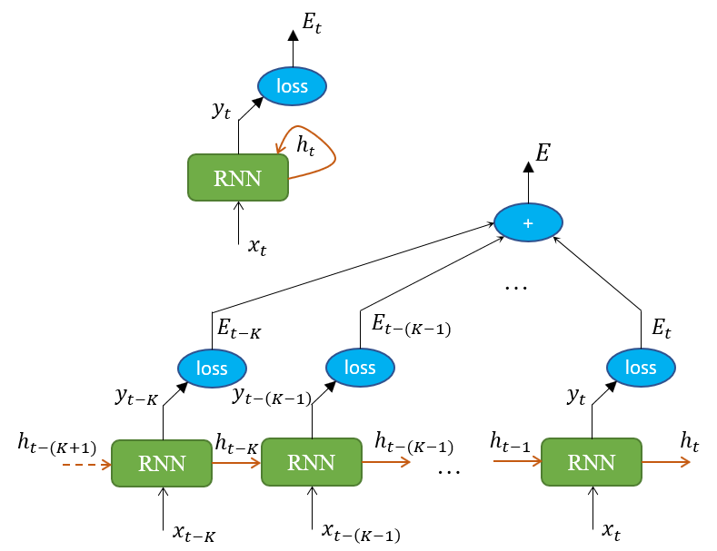
Figure 2: An unrolled RNN with input sequence of K steps with $\tilde{y}_{\tau}$ and $E_{\tau}$ representing the prediction and the corresponding loss (error) at time step $\tau$.

The unrolled RNN looks likes a deep FNN (DNN), but the weights are shared across the units over time. It is an advantage of RNN over FNN as by unrolling the RNN, one obtains a DNN of the same number of layers but with much fewer parameters. Unfortunately, this also leads to disadvantages of RNN, which can be understood in the following. The gradient of the loss $E$ at output with respect to a parameter $\theta$ can be written as

$$\frac{\partial E}{\partial\theta}=\sum_{\tau=1}^{K}\frac{\partial E_{\tau}}{\partial\theta},$$ (6)

where

$$\frac{\partial E_{\tau}}{\partial\theta}=\sum_{j=1}^{\tau}\frac{\partial E_{\tau}}{\partial\tilde{y}_{\tau}}\frac{\partial\tilde{y}_{\tau}}{\partial h_{\tau}}\frac{\partial h_{\tau}}{\partial h_{j}}\frac{\partial h_{j}}{\partial\theta}.$$ (7)

The parameters in the RNN are updated through the backpropagation of the calculated gradients. The backpropagation of the gradients from time $\tau$ are done through all possible routes toward the past, which is also known as backpropagation through time (BPTT).

One disadvantage on BPTT is the computation efficiency because at any time step $\tau$, the calculation of the loss $E_{\tau}$ depend on all previous quantities. It can be seen that with BPTT, the longer the sequence with which the RNN is trained, the more challenging the computation becomes considering both the degraded convergence rate and the increased demand on computing resources. Another numerical issue associated with the gradients with BPTT is that as the span of the temporal dependencies increases, the gradients tend to vanish or explode. The Jacobian term in the gradient of the loss function, ${\displaystyle\frac{\partial h_{\tau}}{\partial h_{j}}}$ in Equation (7) can be proved to be upper bounded by a geometric series [25]:

$$\left\|\frac{\partial h_{\tau}}{\partial h_{j}}\right\|<\gamma^{\tau-j},$$ (8)

where $\gamma$ is a constant determined by the norm of the nonlinearity in RNN. When the hyperbolic tangent function $\tanh$ is chosen as the activation function, we have $\gamma\!=\!1$, and for the sigmoid function, $\gamma\!=\!0.25$ [25]. Therefore, the gradient either explodes or vanishes. We can use a numerical experiment to demonstrate the gradient vanishing and explosion. As shown in Figure 3, an input signal whose magnitude ranges from $-10$ to $10$ is passed through various types of activation functions in multiple times. After the third time, the signal is flattened when the sigmoid function is taken as the activation function. Due to the vanishing of the gradients, the sigmoid function cannot be used as the activation function in a RNN unit. In contrast, as shown in Figure 3(c) when ReLU is taken as the activation function, the signal remains as its original shape after being passed through the unit for iterations, which is also the reason why ReLU is very popular in modern RNN structures.

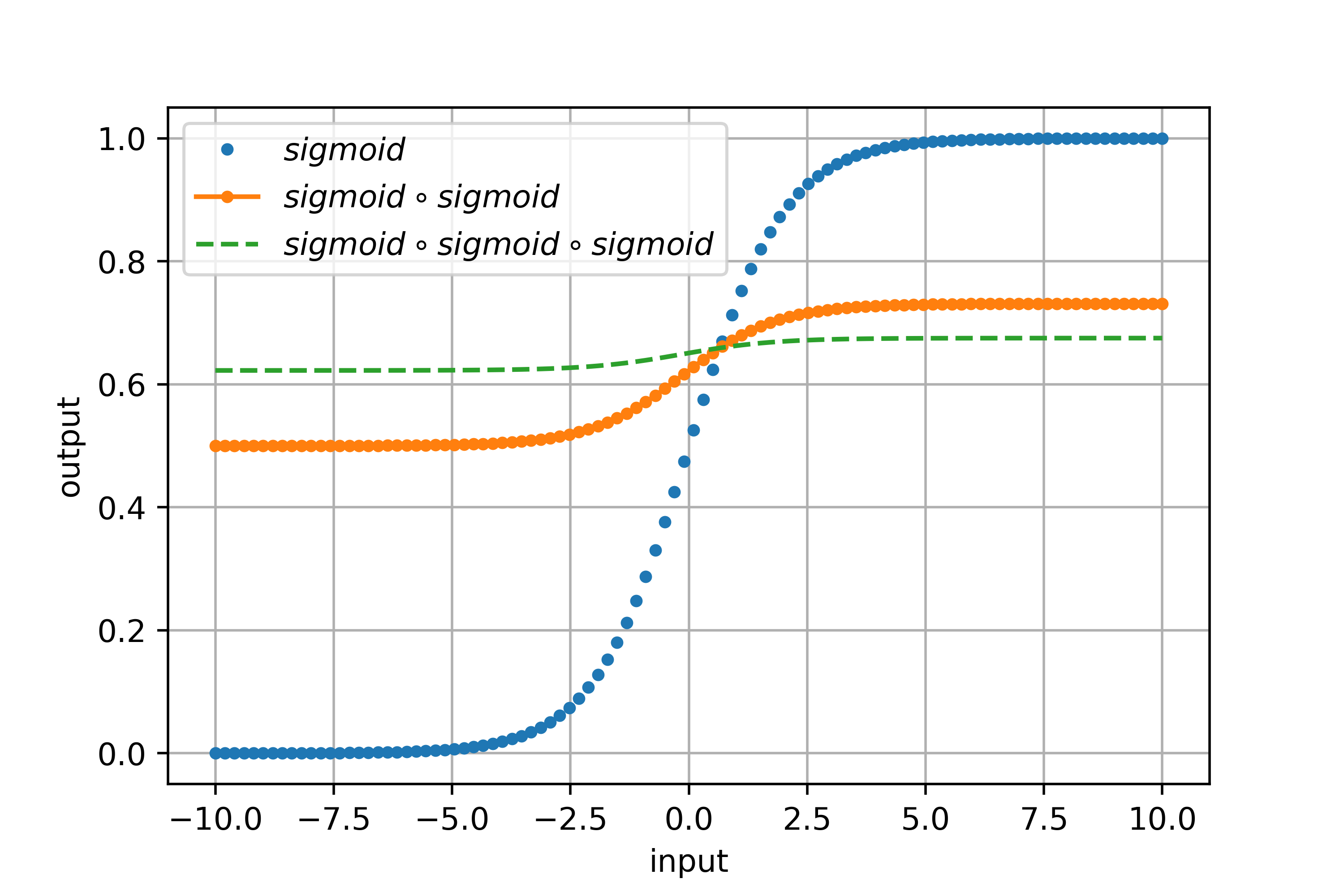
(a) Sigmoid

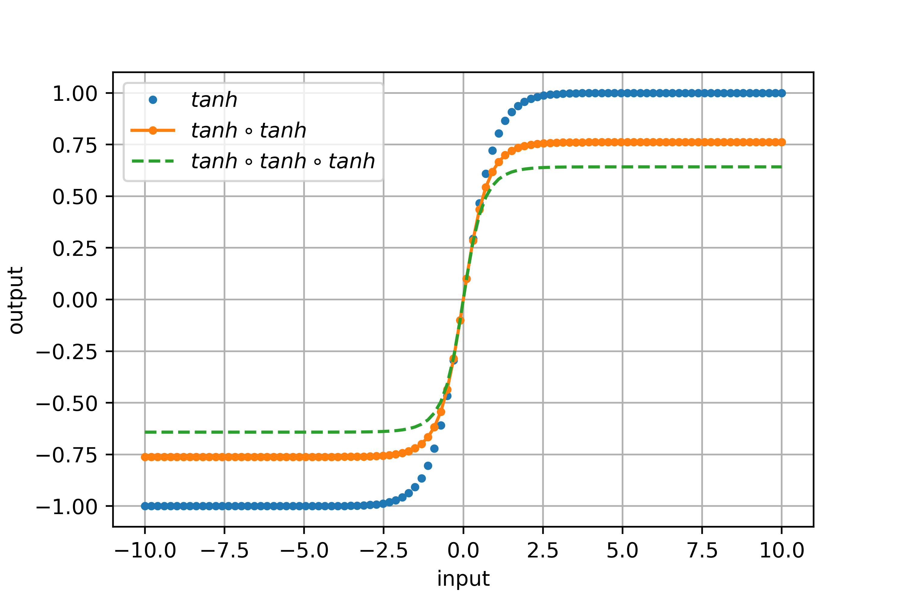
(b) Tanh

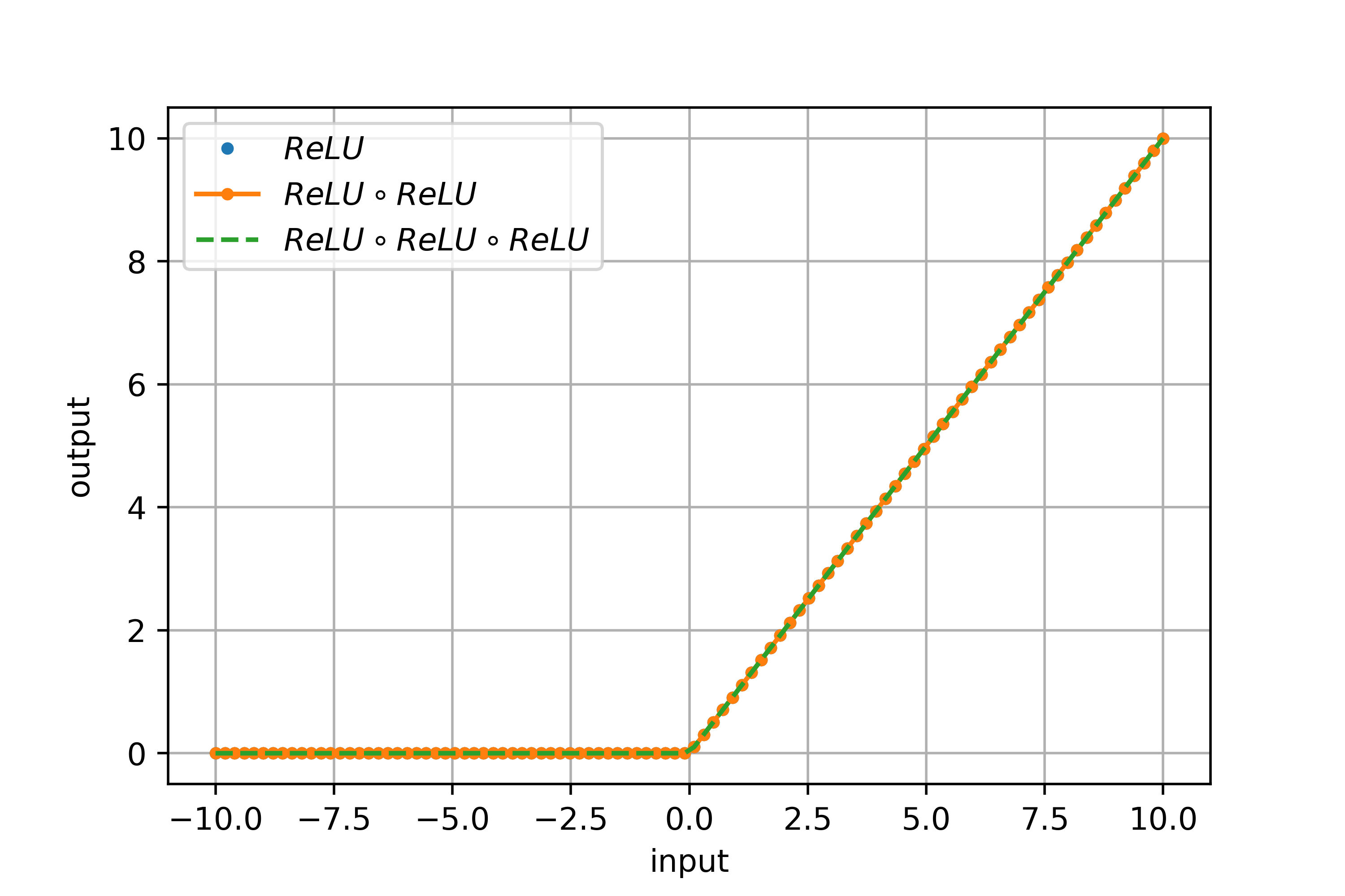
(c) ReLU

Figure 3: Multiple passes through the same activation function.

One remedy to the problem of gradient vanishing or exploding is known as truncated backpropagation through time (TBPTT) [26, 27], which is a modified version of BPTT. A TBPTT processes the sequence one step at a time, and after every $k_{1}$ time steps, it calls BPTT for $k_{2}$ time steps. A common configuration of TBPTT is that the forward and backward processes share the same number of steps such that $k_{1}\!=\!k_{2}$. Another remedy utilizes a more sophisticated activation function with gating units to deal with problem of gradient vanishing or explosion, for example, the long short-term memory (LSTM) unit [28] and the gated recurrent unit (GRU) [29]. Both LSTM unit and GRU own gates, which allow the RNN cell to forget. The working mechanism of a LSTM network is based on

$$\left\{\begin{array}[]{ccl}i_{t}\!\!\!\!&=&\!\!\!\!\sigma\left(W_{ii}x_{t}+W_{hi}h_{t-1}\right)\\ f_{t}\!\!\!\!&=&\!\!\!\!\sigma\left(W_{if}x_{t}+W_{hf}h_{t-1}\right)\\ g_{t}\!\!\!\!&=&\!\!\!\!\tanh\left(W_{ig}x_{t}+W_{hg}h_{t-1}\right)\\ o_{t}\!\!\!\!&=&\!\!\!\!\sigma\left(W_{io}x_{t}+W_{ho}h_{t-1}\right)\\ c_{t}\!\!\!\!&=&\!\!\!\!f_{t}c_{t-1}+i_{t}g_{t}\\ h_{t}\!\!\!\!&=&\!\!\!\!o_{t}\tanh\left(c_{t}\right),\end{array}\right.$$ (9)

where $h_{t}$ is hidden state at time $t$, $c_{t}$ is the cell state, and $i_{t},f_{t},g_{t},o_{t}$ are the input, forget, cell and output gates respectively.

As a comparison to a LSTM unit, there is no cell component in GRU and the working mechanism of a GRU network is as follows

$$\left\{\begin{array}[]{ccl}r_{t}\!\!\!\!&=&\!\!\!\!\sigma\left(W_{ir}x_{t}+W_{hr}h_{t-1}\right)\\ z_{t}\!\!\!\!&=&\!\!\!\!\sigma\left(W_{iz}x_{t}+W_{hz}h_{t-1}\right)\\ n_{t}\!\!\!\!&=&\!\!\!\!\tanh\left(W_{in}x_{t}+r_{t}W_{hn}h_{t-1}\right)\\ h_{t}\!\!\!\!&=&\!\!\!\!\left(1-z_{t}\right)n_{t}+z_{t}h_{t-1},\end{array}\right.$$ (10)

where $z_{t}$ and $r_{t}$ are called the update and the reset gates. Both $z_{t}$ and $r_{t}$ function as control signals within the unit. The GRU employs a new way to calculate the memory $n_{t}$ by using the current input and the past hidden state. It can be seen that a LSTM unit requires a more complex implementation on the gating functions than a GRU. However, both LSTM unit and GRU are able to store and retrieve relevant information from the past by using gating control signal, which resolves the issue of gradient vanishing or explosion [28].

III Training an RNN

In this section, we will review three different training schemes, namely, readout, teacher force, and professor force. The most trivial way to train an RNN is the readout training as shown in Figure 4. By taking advantage of the recurrent nature of an RNN, the readout training takes the output at previous time steps as the input. The ground-truth $\tilde{y}_{k}$ is only used in calculating loss with the corresponding prediction $y_{k}$. The RNN is fed with what it generated, which is also the reason it is called readout. Readout technique is mostly adopted in inference, i.e. when predictions are being made on the unseen data. However, training in readout mode often takes longer time on convergence because the model has to make a lot of mistakes, being penalized for many times before it eventually learns to generate accurate predictions. Therefore, teacher force training is often preferred over readout. In teacher force training as illustrated in Figure 5, the ground-truth values are fed into an RNN as input. Teacher forcing can ensure an RNN learn faster but not necessarily better.

Figure 4: Readout training.

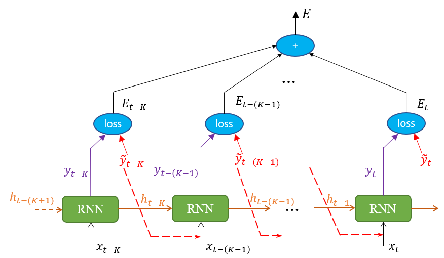
Figure 5: Teacher force training.

Similar to the mechanism behind overfitting, the underlying distribution of the input data in teacher force training may be very different from that during its readout mode inference. In that case, teacher force training may have worse performance on unseen data comparing to its performance on the training set. To filter out the potential bias in training, a scheduling process can be adopted [30]. A good analogy of the scheduling process is the event of flipping a coin: we can imagine that a coin is flipped every time before the previous output is fed into an RNN as the input. The coin used in the scheduling process is biased: for the first few training epochs, the coin is biased towards the training data distribution such that the training is more into a teacher force mode; as the training evolves, the coin becomes biased towards the distribution of the predicted data, in other words, in a readout mode. The scheduling technique has lead to a significant improvement on the generalization capability of an RNN model in speech recognition [31]. In this paper, we use the teach force training with scheduling for the transient channel simulation example shown in Section IV.

There is an another training scheme called professor force [32] technique which enforces the similar behaviors of the network during training and test. The professor force training uses the concept from generative modeling, to be specific, generative adversarial network (GAN) to fill the gap between the training distribution and the predictive distribution, providing better generalization performance.

IV Numerical examples

The robustness of the proposed method using RNN to model high-speed channels will be illustrated through two different types of RNN presented in Section II using a PAM2 and a PAM4 driver circuit. Different training conditions such as optimization method, memory length and recurrent cell topology etc. will be investigated.

IV-A PAM2 channel simulation with output-feedback RNN (NARX-RNN)

In this section, we illustrate the training procedures of the RNN, with which the predictions can be made on the voltage waves arriving at the receiver of a high-speed channel using NARX-RNN. As demonstrated in Equation (3), the NARX-RNN does not have a hidden state explicitly defined in the model. The current output response is determined only using the current and past values of the input and the past values of the output. The set up is shown in Figure 6: $V_{TX0}$ is the output voltage of the transmitter (TX) when it is terminated with a 50 Ohm resistor; and $V_{TX}$ and $V_{RX}$ are voltages at the immediate output of TX and the input of RX in the presence of the channel. In this example, we use $V_{TX}$ and $V_{TX0}$ of the current time step and $V_{RX}$ of the past to predict $V_{RX}$ of the current time step.

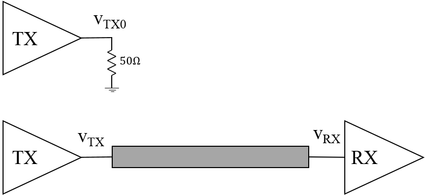
Figure 6: Simulation setup for data collection..

The data is normalized and segmented into sequences of length $K$. Sample sequences after normalization of all the signals of interest are depicted in Figure 7. This number $K$ represents the memory dependency of the system. The larger the $K$ is, the longer the memory the system keeps. A portion of the data ($10\%$) is reserved for test. In this example, a stack of four LSTM cells of 20 hidden units is used. The optimization method used is Adam with 0.3 dropout regularization. Throughout our experiments, increasing $K$ not only improves the convergence but also achieves higher accuracy. However, once $K$ reaches the underlying memory length of the system under learning, a further increase does not offer better convergence nor higher accuracy. We use $K=10$ in the following numerical experiments. The time steps for training is 11,000 and the model converges in about 48 epochs. Accurate predictions are achieved on unseen sequence as shown in Figure 8.

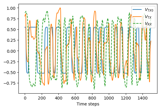
Figure 7: Training data collected with the setup shown in Figure 6.

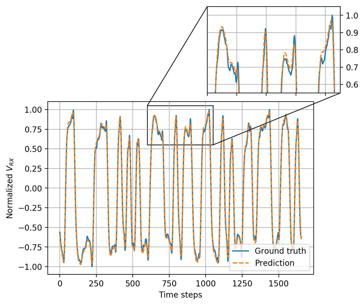
Figure 8: Predicted voltage at the receiver $V_{RX}$ with a LSTM network.

Figure 9 and Figure 10 show the comparison between LSTM network and vanilla RNN in terms of their capability of handling the long-term memory. The same network architecture is adopted in this comparison including the number of layers, the layer width, and the regularization. It is shown that when the memory is relatively short with $K=4$, the vanilla RNN cells fails to capture the signal evolution whereas the LSTM network makes pretty accurate predictions. When the memory is sufficiently long, the vanilla RNN starts making comparably accurate predictions as the LSTM network does, which is shown in Figure 10. From this comparison, it also reveals that training with Adam optimizer achieves better performance than the SGD optimizer regardless of the memory length.

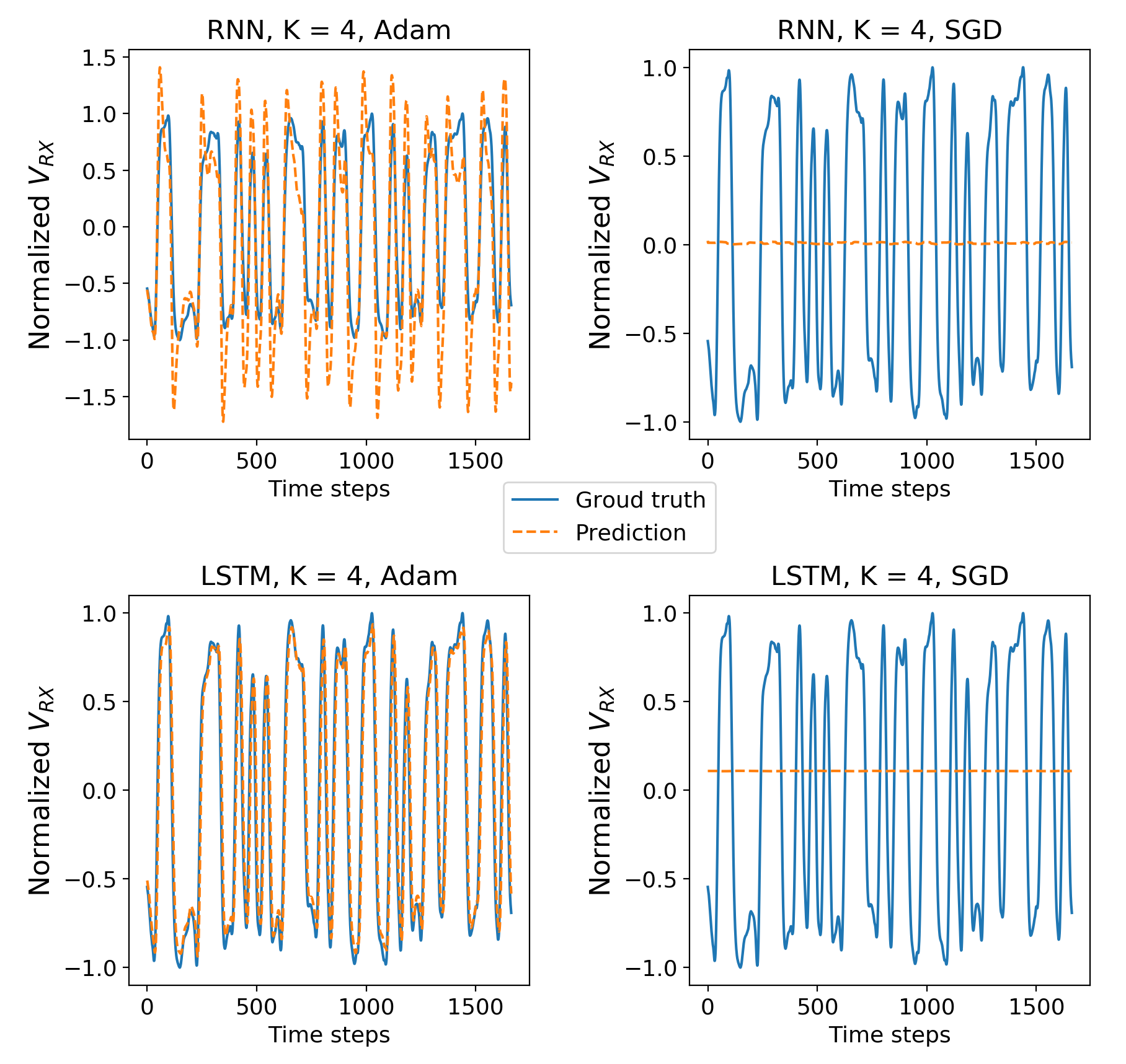
Figure 9: Comparison between vanilla RNN and LSTM network in handling relative short memory when the memory length $K$ is chosen as 4.

It is worth mentioning that while using the LSTM and GRU networks, one needs to pay particular attention upon the selection of activation functions. For example, the gating signals $f_{t}$ and $i_{t}$ in Equation (9) controls the percentage of the memory passing through the gates, which ranges from 0 to 1. In this case, the activation function associated with $f_{t}$ and $i_{t}$ has to be the sigmoid function. Besides, the gating signal $g_{t}$ in Equation (9) allows both addition and subtraction operations between the input and the forget gates and the hyperbolic tangent function is appropriate. As for a VRNN, the selection of activation functions is only based on the nonlinearities. As shown in Figure 11, using the hyperbolic tangent function as the activation function in a vanilla RNN achieves more accurate predictions than that with ReLU.

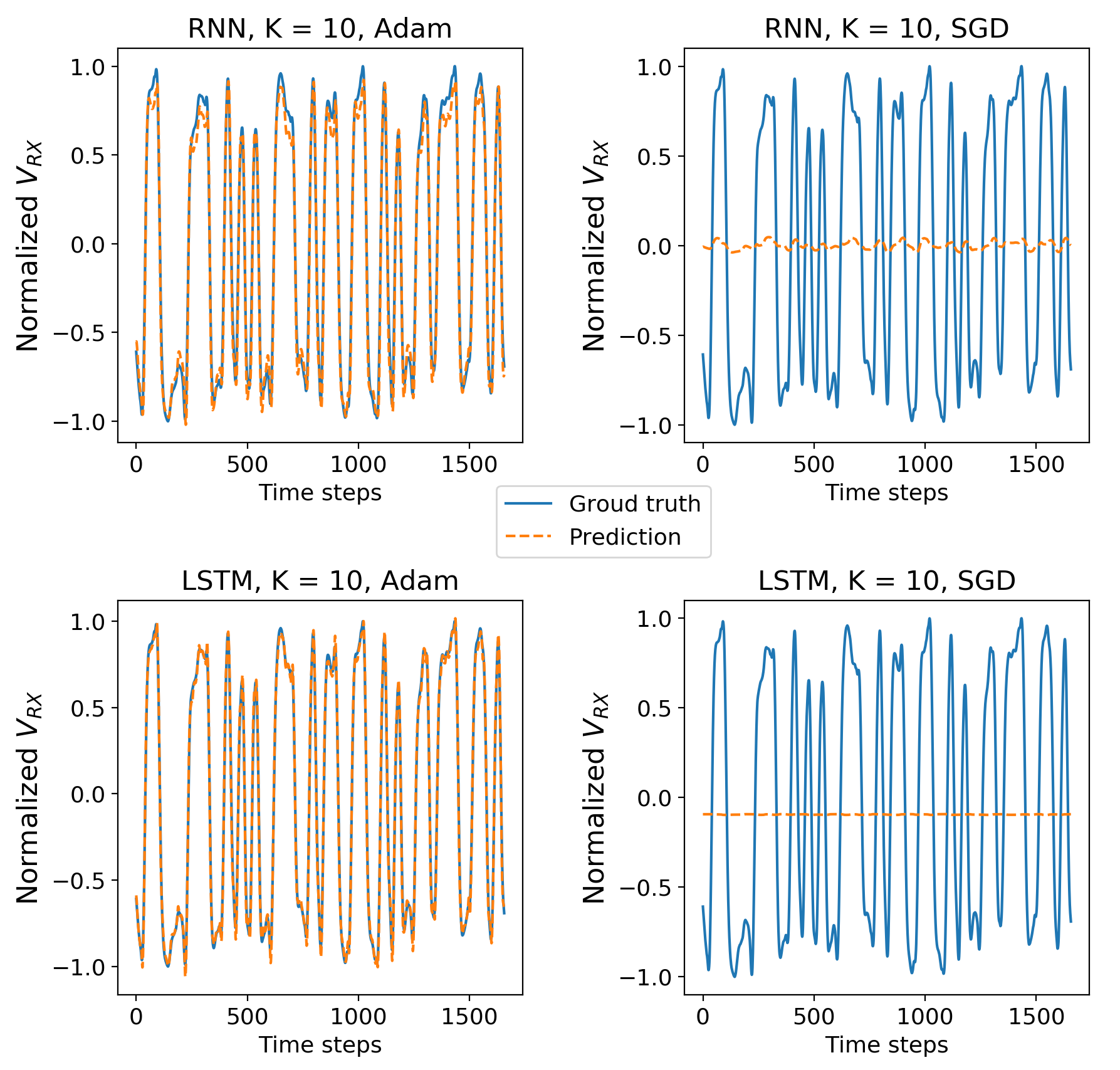
Figure 10: Comparison between vanilla RNN and LSTM network in handling sufficiently long memory when the memory length $K$ is chosen as 10.

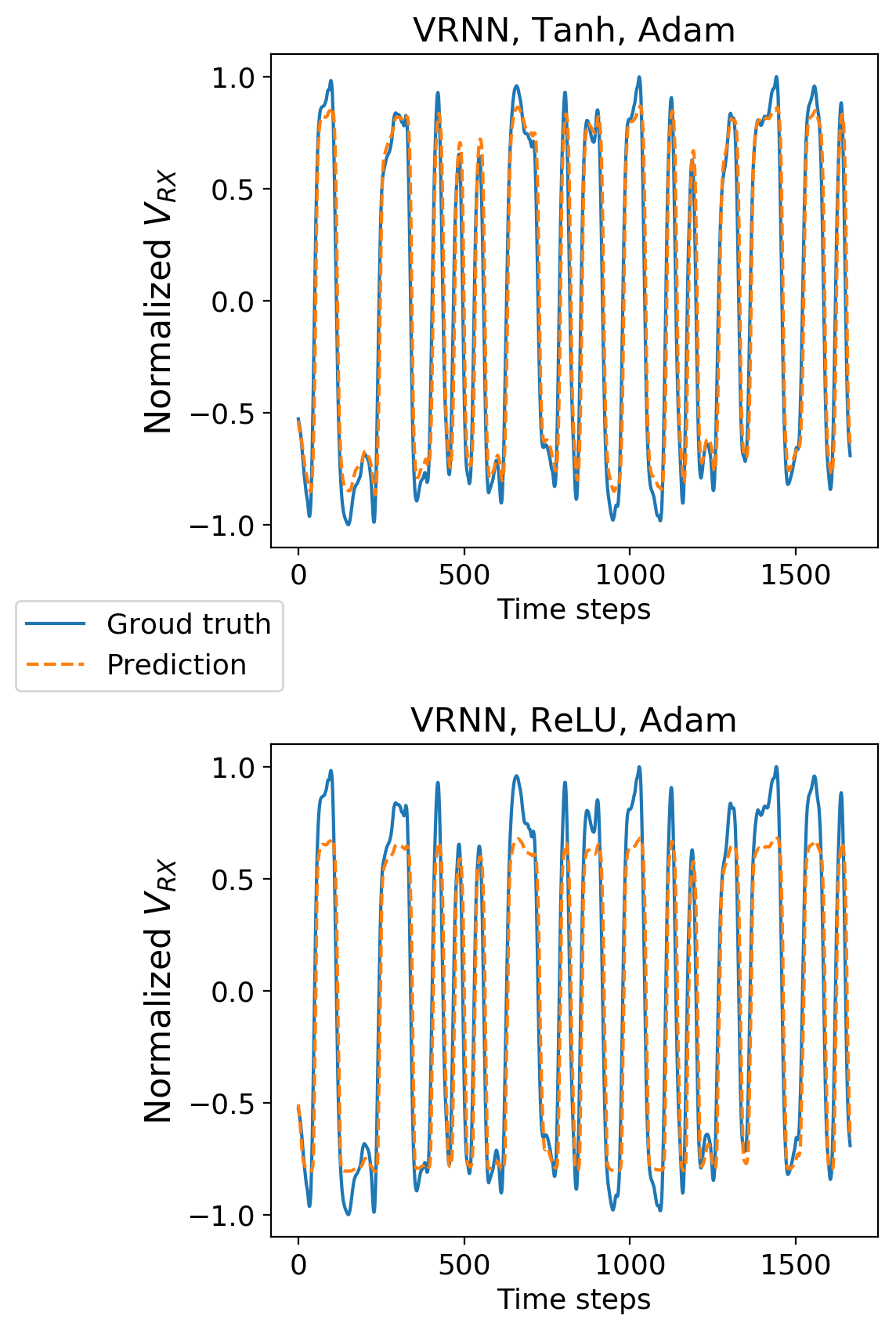
Figure 11: The impact from different types of activation functions on the prediction accuracy in a vanilla RNN.

In addition, SGD optimizer does not work for the proposed RNN structure under the aforementioned settings for training. Adding momentum for SGD does not help the learning process either. However, Adam optimizer achieves accurate predictions. We also investigate RMSProp optimizer, which has been used for RNNs long before Adam is invented, to train the same architecture in terms of both VRNN and LSTM network. It is found that for short memory such as $K=4$, using RMSProp optimizer does not achieve convergence; as the memory length $K$ goes beyond 5, RMSProp optimizer performs as well as Adam. The result shown in Figure 12 confirms that for $K=5$, networks trained by RMSProp make accurate predictions on the output waveform. However, setting a high momentum to deploy adaptive learning rate degrades the performance of the network; as can be seen in Figure 12, the prediction accuracy becomes worse with momentum added in RMSProp.

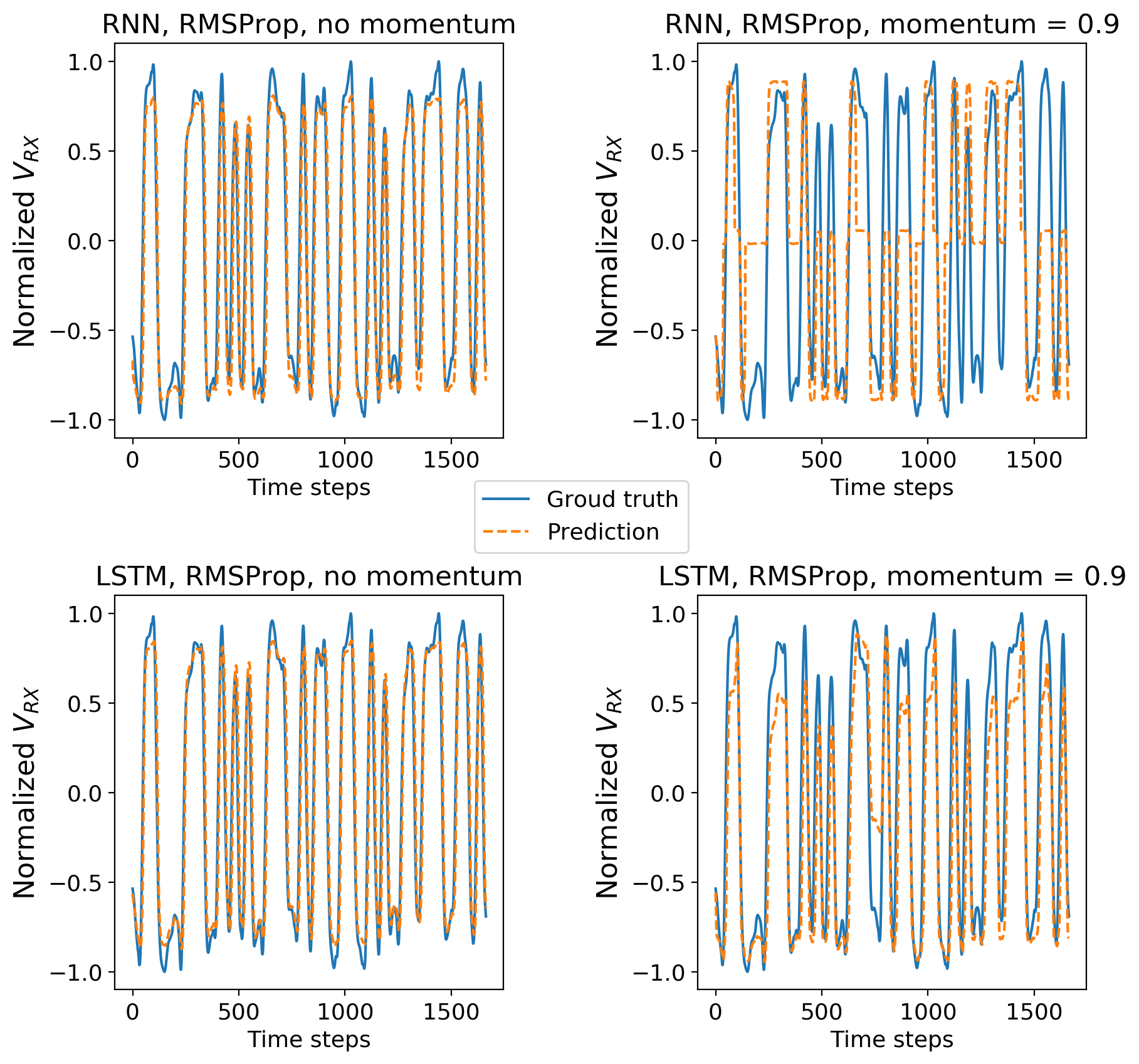
Figure 12: Performance of the same architecture using different RNN cells, trained by RMSProp when $K=5$

IV-B PAM4 channel simulation with ERNN

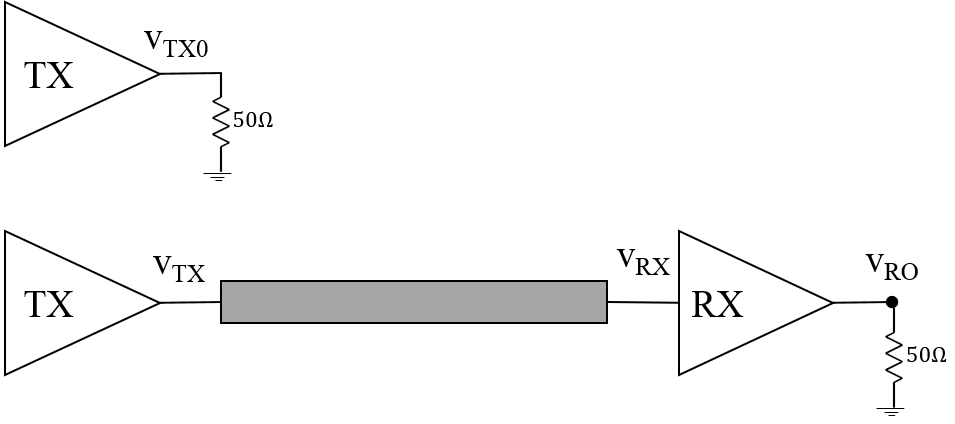
Figure 13: Setup to obtain training data for PAM4 example.

The limitation of the output-feedback RNN used in the PAM2 example is that it strictly requires the output of the current time step before it can make predictions on one future time step, which can be seen from Equation (3). The neural network model, while being used in this way, cannot utilize batch inference. In this example, it is shown that using a deeper and wider network, an RNN-based model can be developed to utilize batch inference, which can dramatically reduce the run time for long transient simulation.

To prepare the training data, first, the transmitter output is measured when it is opened, denoted as $V_{TX0}$. This signal is the Thevenin source to the combined “channel and receiver” system of interest. When the transmitter is connected to the channel and the receiver, the input to the channel from the transmitter $V_{TX}$ and the input to the receiver after the channel $V_{RX}$ are both collected for training purpose. Besides, the output voltage from the receiver $V_{RO}$ is also captured and included in the training set. The setup for data collection is shown in Figure 13. The data in this example comes from a PAM4 transceiver circuit transmitting data at 28 Gbps. An LSTM network is trained on about $10,000$ time points of time domain response of as shown in Figure 14. A training waveform sample is shown in Figure 15.

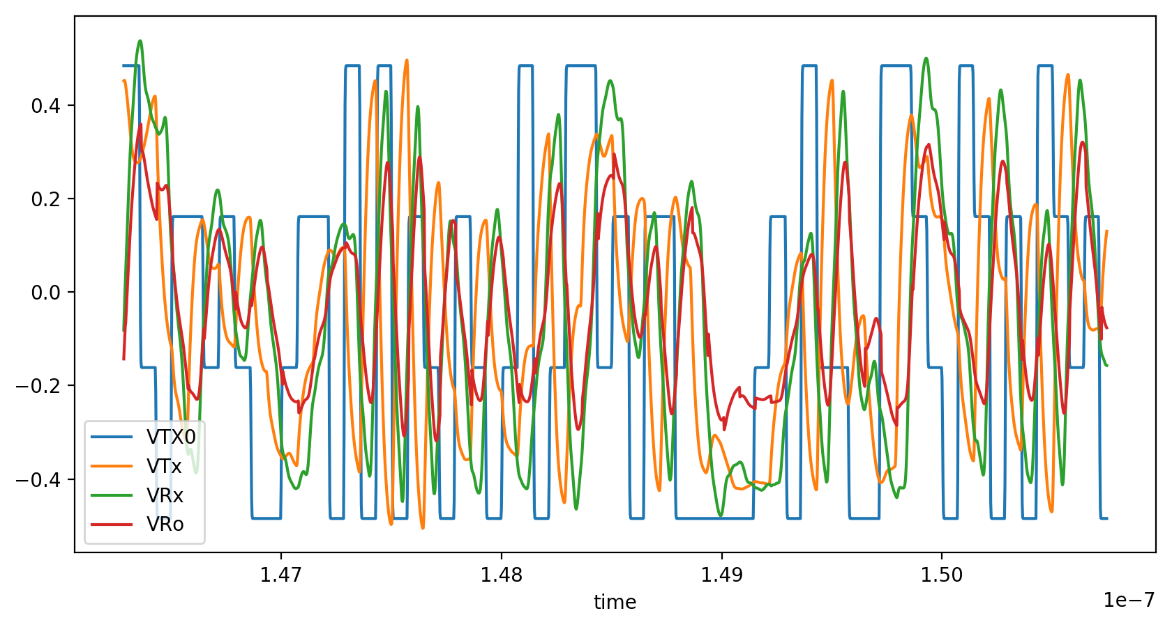
Figure 14: Voltages used to train ERNN in PAM4 example.

We first investigate the impact from memory length on the training process. The memory length depends on not only the nonlinearity of the transmitter and receiver but also the delay of the channel. As for the training setup, Adam is used as the optimizer with initial learning rate of 0.001 and dropout regularization is fixed at 0.3. The LSTM network has six layers each with 30 hidden units. The memory length $K$ is varied with everything else remaining the same. Figure 16 demonstrates the training performance under various memory lengths with the same network topology. By showing the results at different epochs, Figure 16 also reveals the fact that the learning ability of the LSTM network evolves as the training progresses. For example, at the $100^{\textrm{th}}$ epoch, the LSTM network learned the switching pattern of the waveforms; at the $1000^{\textrm{th}}$ epoch, the same network is able to make accurate predictions on $V_{TX}$ in terms of both the pattern and the amplitude.

With the memory length chosen as $K\!=\!50$ and at the $1000^{\textrm{th}}$ epoch, the predictions made with the LSTM network on $V_{RO}$ are less accurate than those on $V_{TX}$, as shown in Figure 16. The reason that obtaining accurate predictions on $V_{RO}$ is more challenging than that for $V_{TX}$ is because the former requires a much better knowledge of the delay imposed by the channel. It seems the memory length set by $K\!=\!50$ dose not provide adequate data on the channel delay. After the memory length is increased to $K=90$, the predictions on $V_{RO}$ become much more accurate, as shown in Figure 16c. A further increase of the memory length to $K\!=\!100$ does not further improve the performance as shown in Figure 16d. It is worth mentioning that the increase of memory length demands more computation resources.

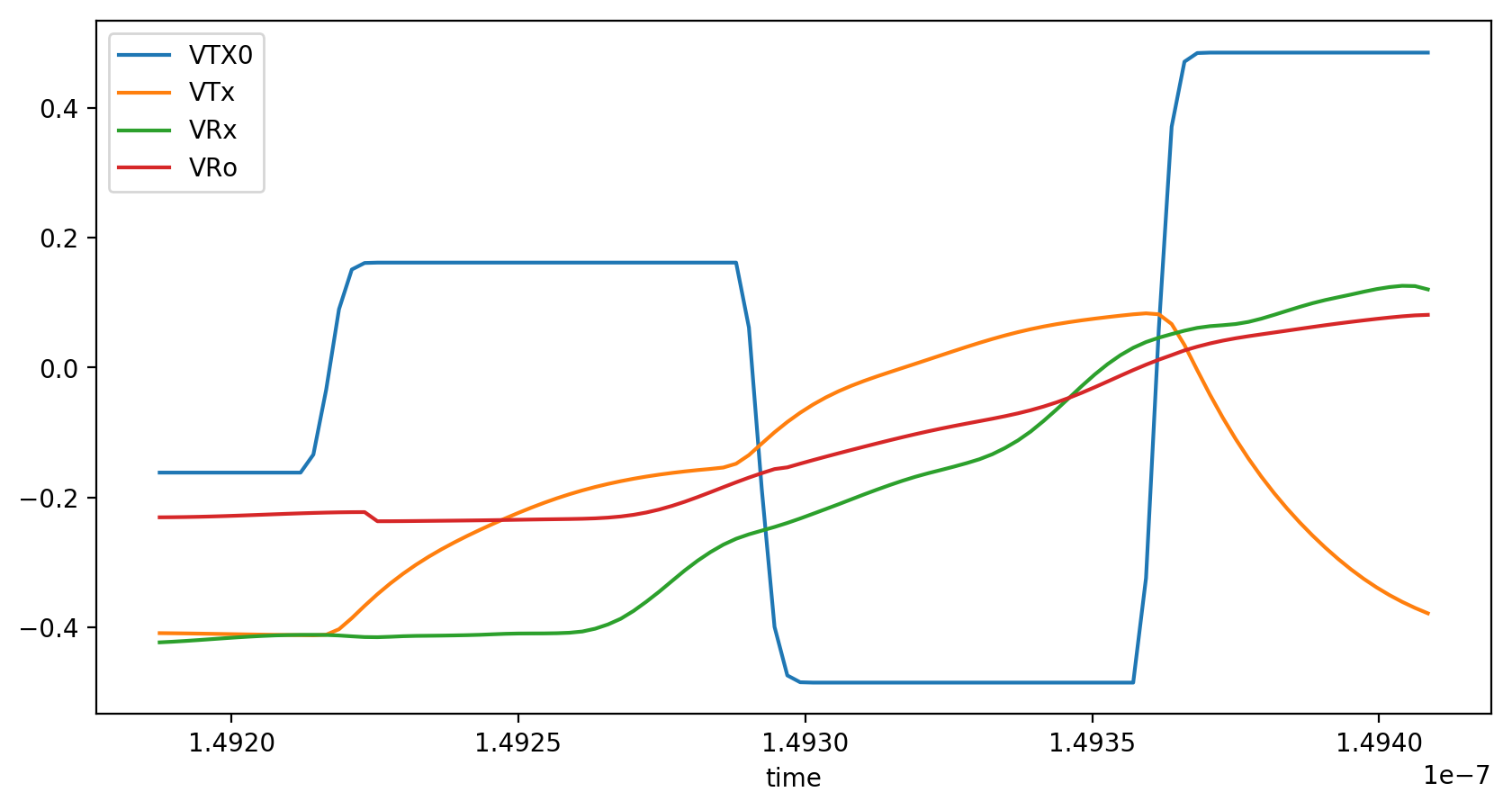
Figure 15: A training sample by windowing the training sequence with $K=100$.

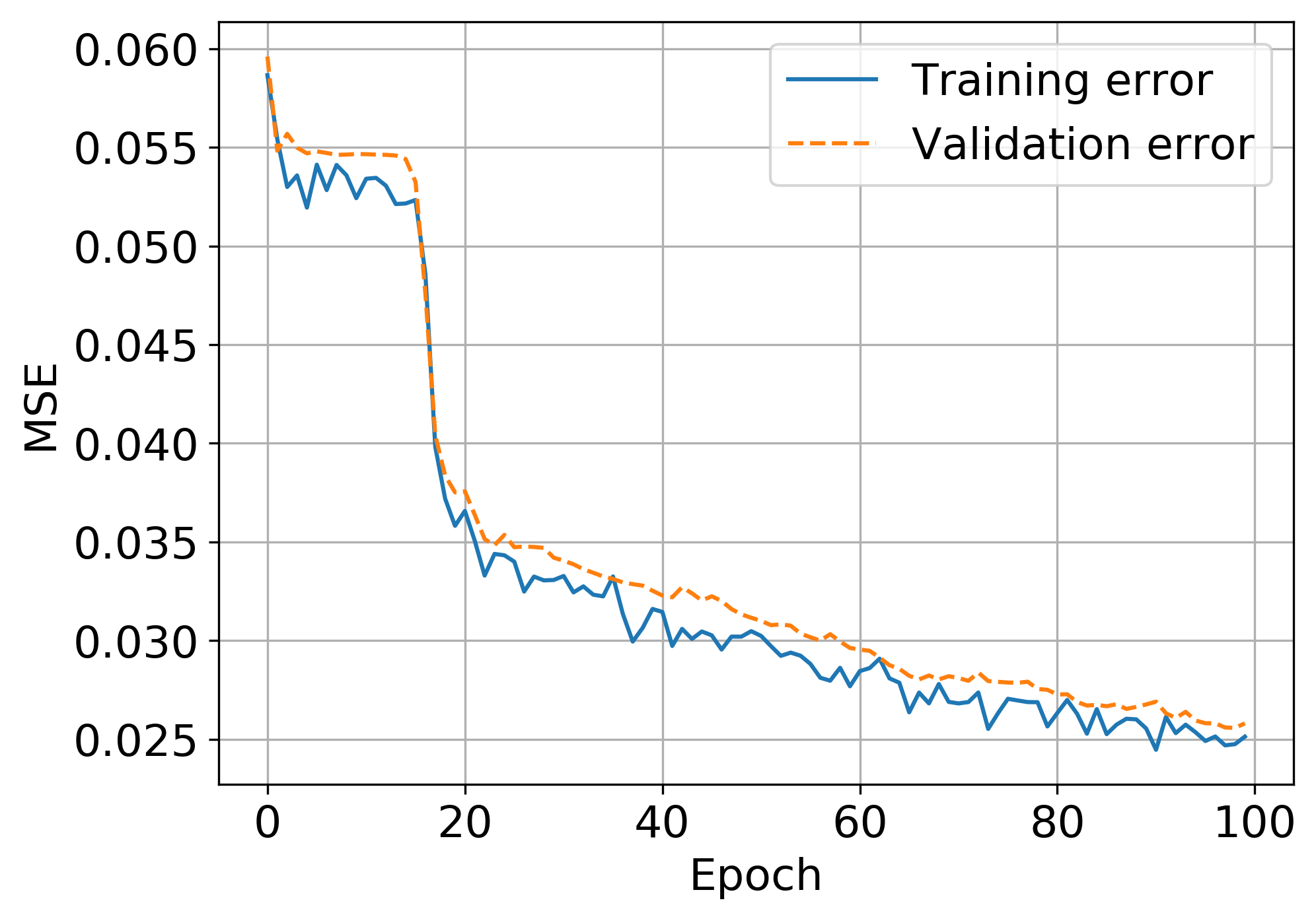
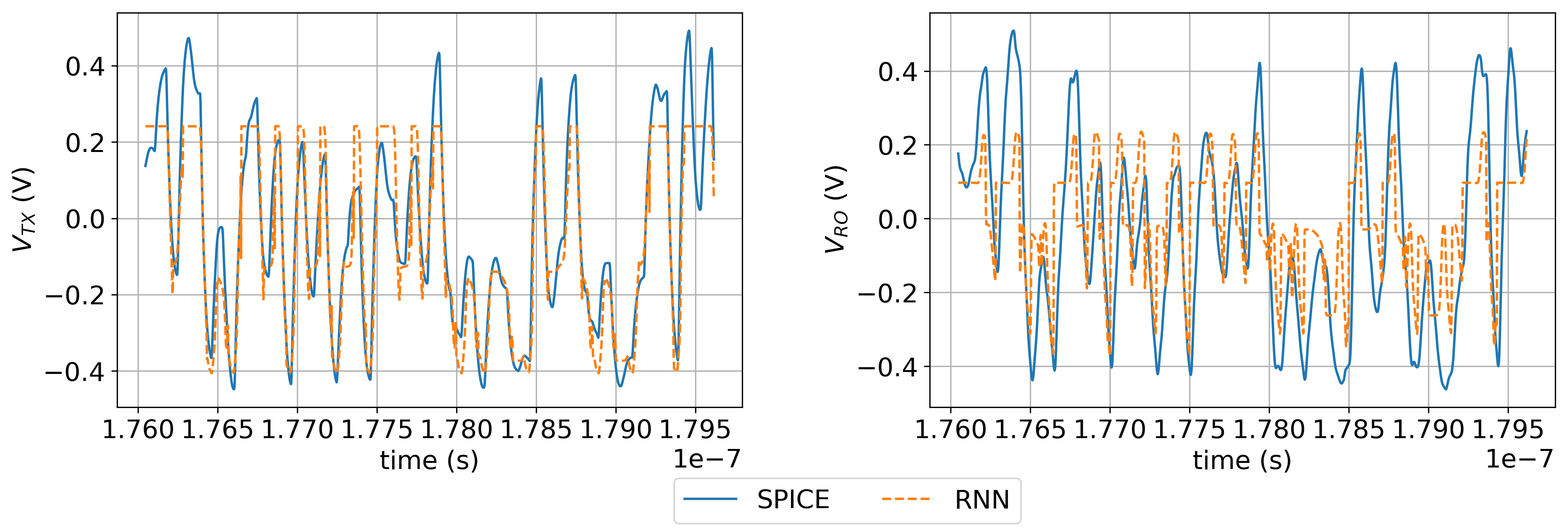
(a) When $K=50$, trained in 100 epochs.

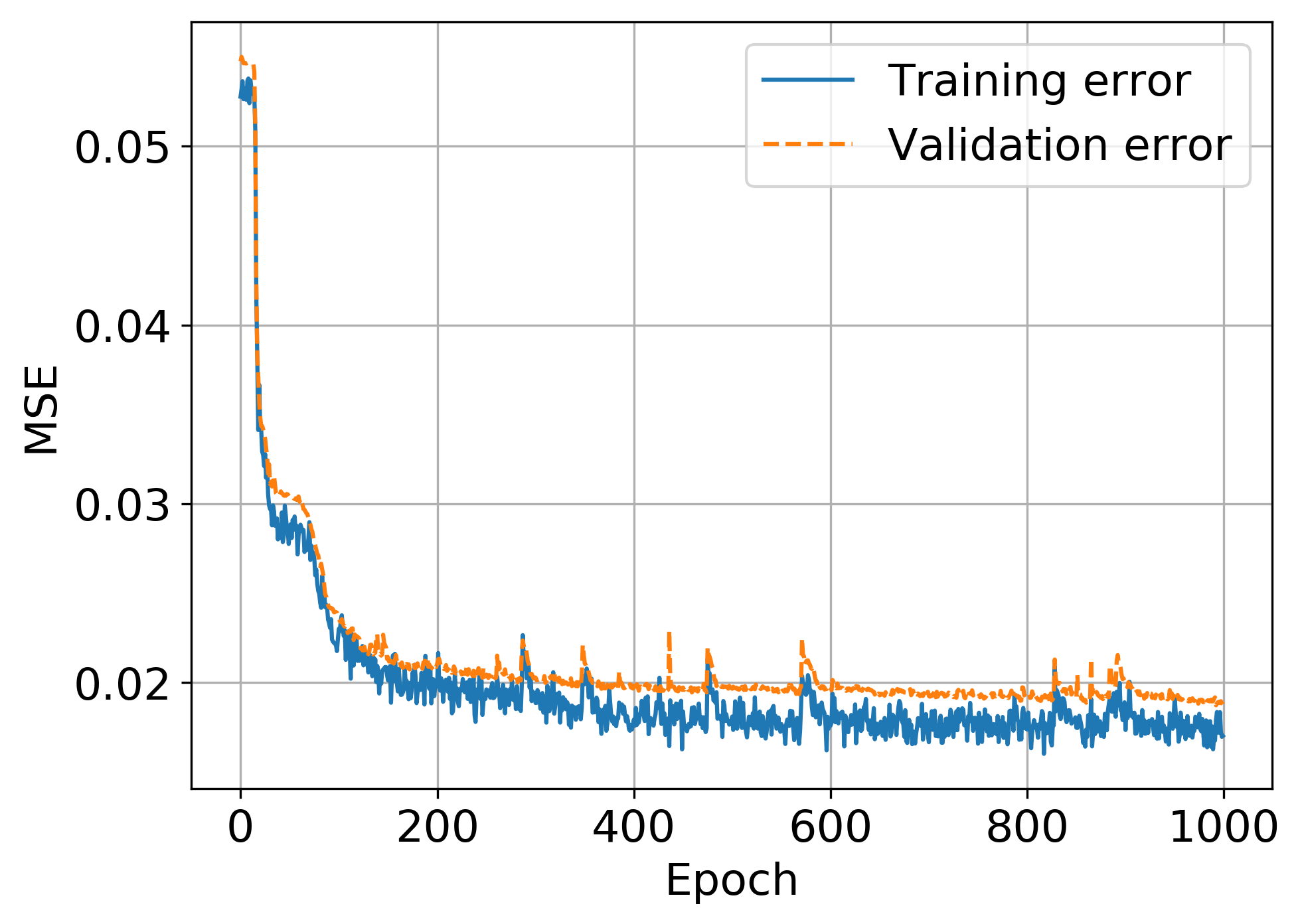
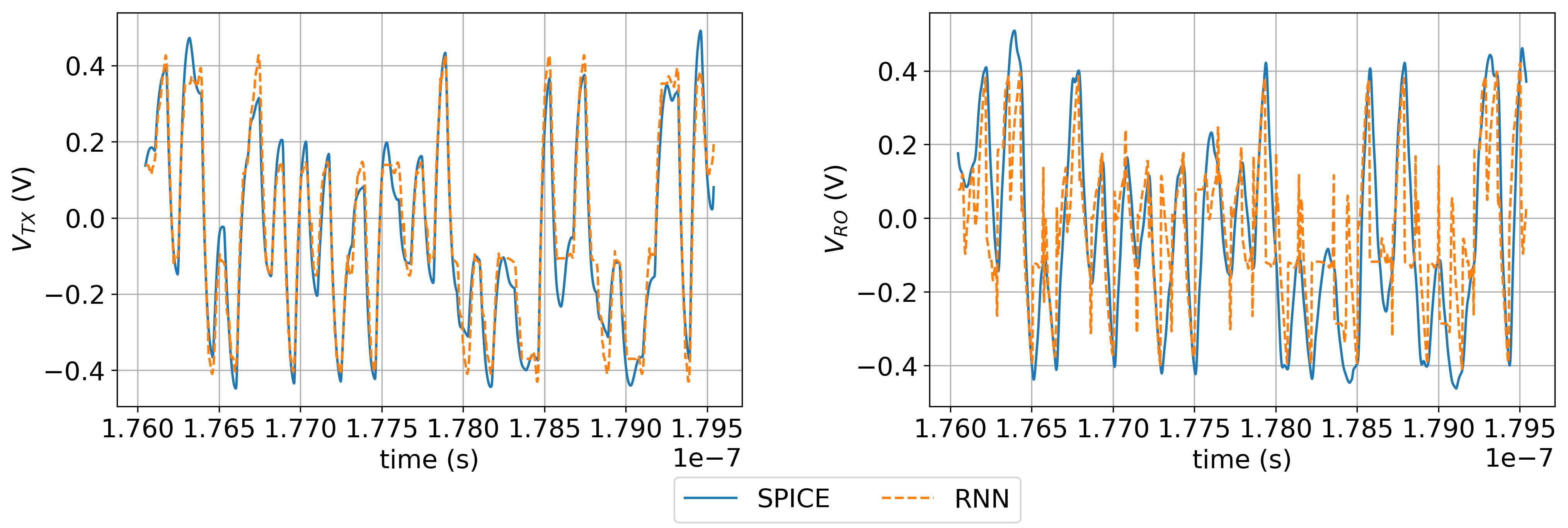
(b) When $K=50$, trained in 1,000 epochs.

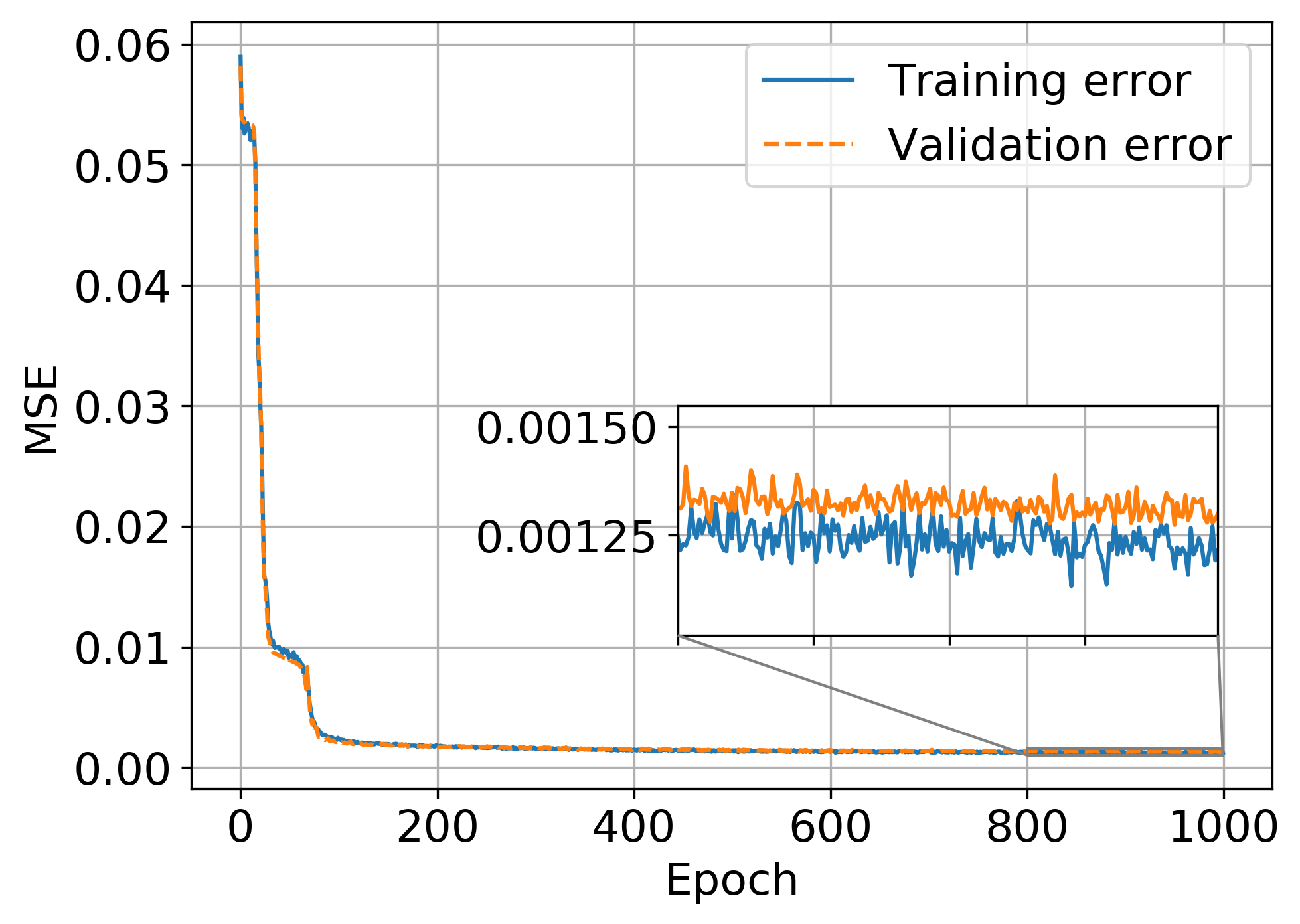
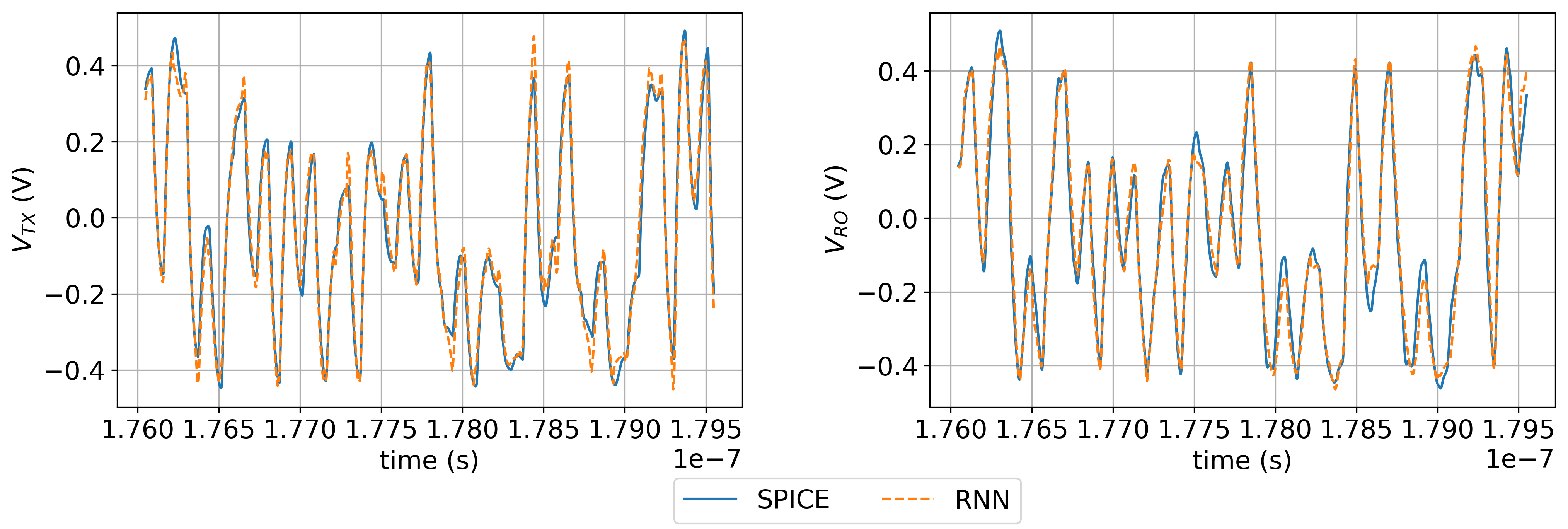
(c) When $K=90$ trained in 1,000 epochs.

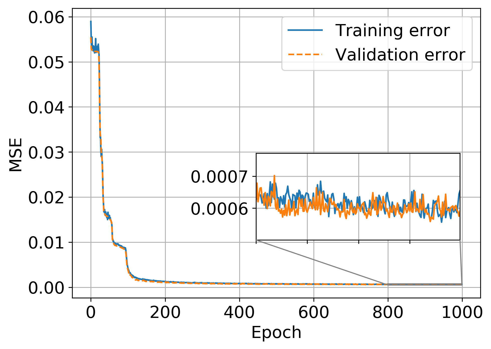
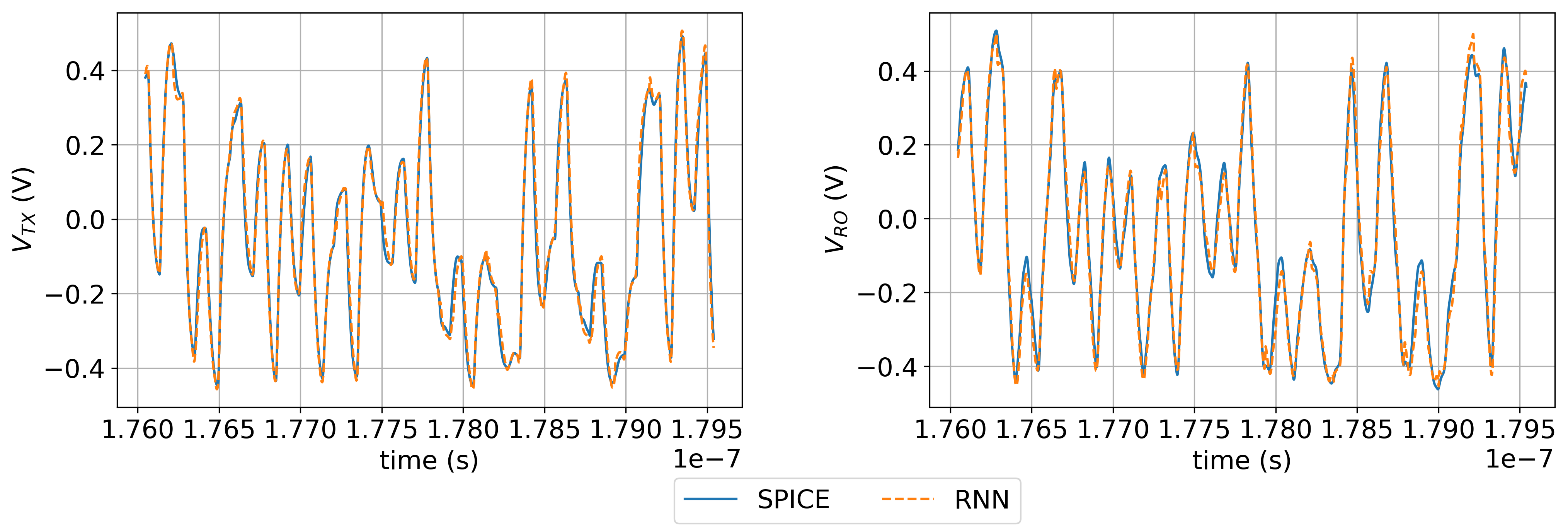
(d) When $K=100$, trained in 1,000 epochs.

Figure 16: Training error (most left) and test performance of RNN model in PAM4 transceiver example.

To further validate the model, we employ a much longer PRBS than the training one and generate eye diagrams. In Figure 17, it shows a very good agreement between the eye diagram generated from traditional SPICE-like simulation and the one from the proposed RNN-based model. For example, both eye diagrams point out that the optimal sampling point is about 14.662 $\mu s$.

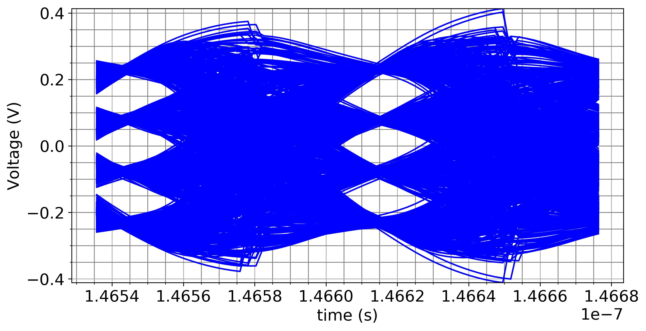
(a) From SPICE

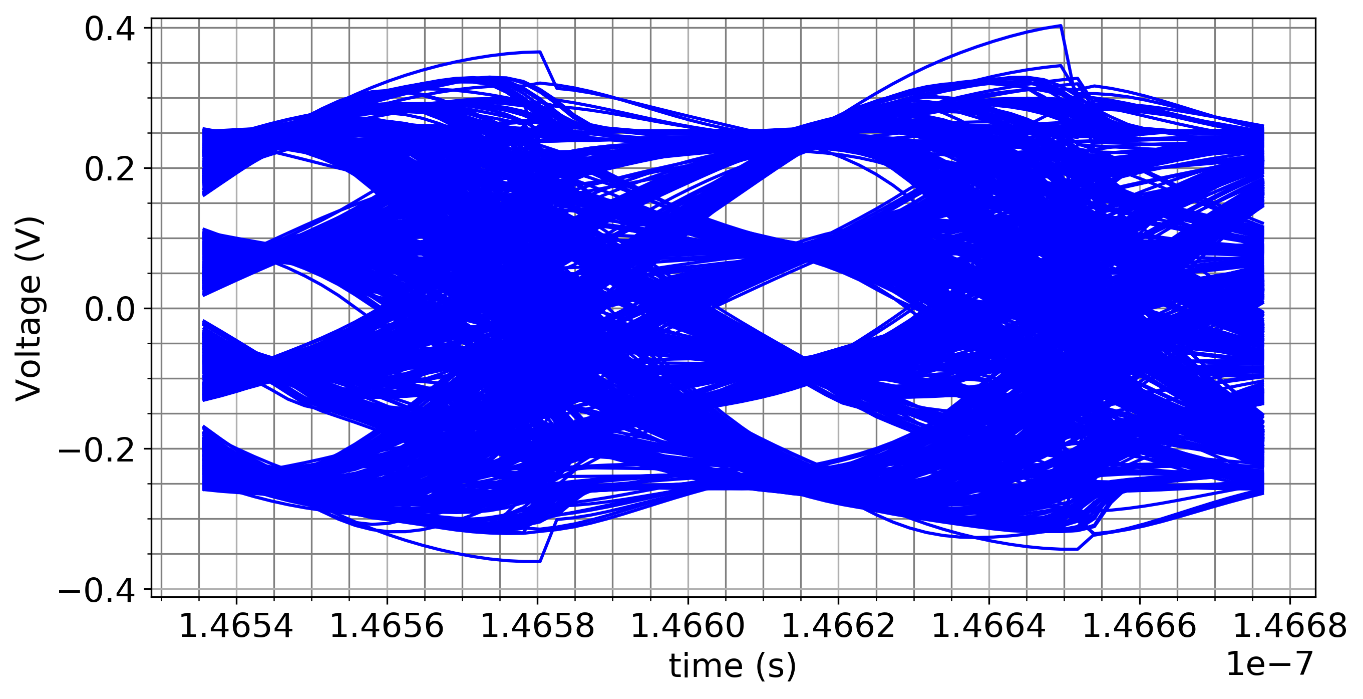
(b) From RNN

Figure 17: Eye diagram obtained in PAM4 transceiver example.

IV-C Accumulation of numerical error

One limitation of the proposed method with RNN is the accumulation of numerical error. During the training process, TBPTT gives a noisy gradient information to the optimizer, which translates to the numerical error in the solution. This numerical error, though initially very small, gradually accumulates as the prediction goes on with the input sequence. A longer input sequence leads to a larger numerical error in the predicted results. Figure 18 shows the performance of the trained model in the previous section on a very long PRBS. Initially, the predicted results from the RNN model agree well with those obtained from the circuit simulation. However, as the prediction progresses, the numerical error due to TBPTT accumulates and degrades the performance of the RNN model. The accumulation of the numerical error is a well-known limitation of RNN trained by TBPTT, which at the same time leaves room for improvement in the future work on the proposed method with advanced techniques for sequence modeling such as attention mechanism [33].

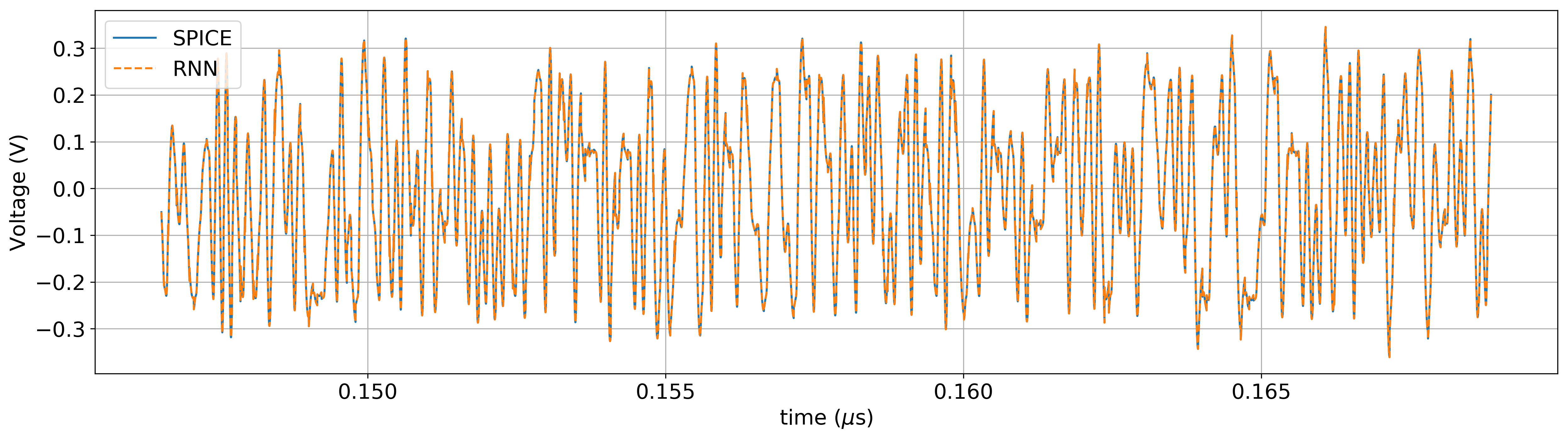
(a) Initially

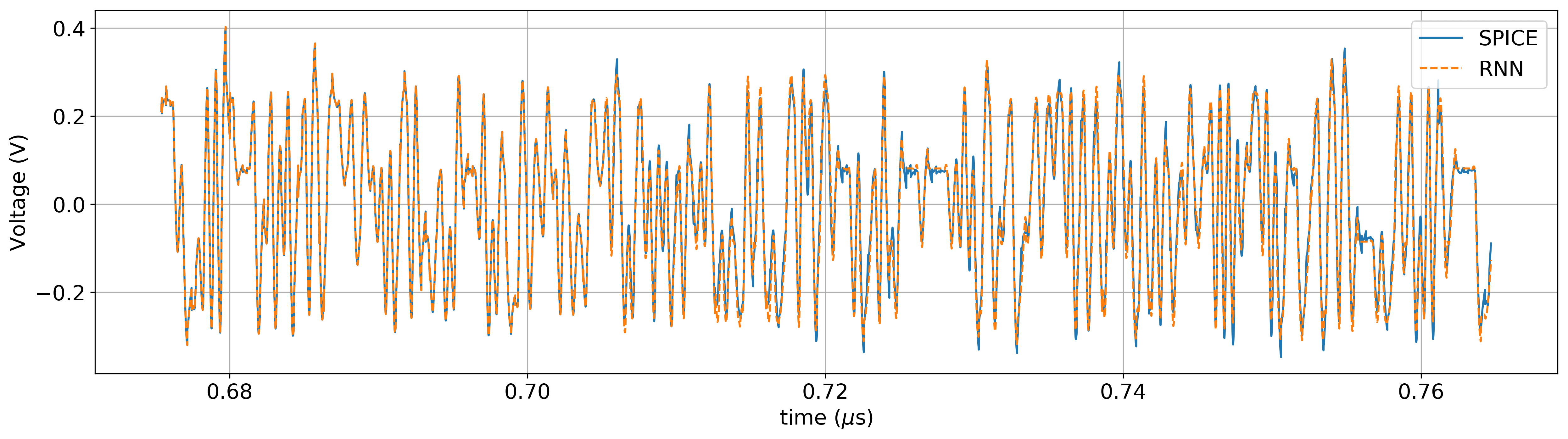
(b) After tens of thousands of bits

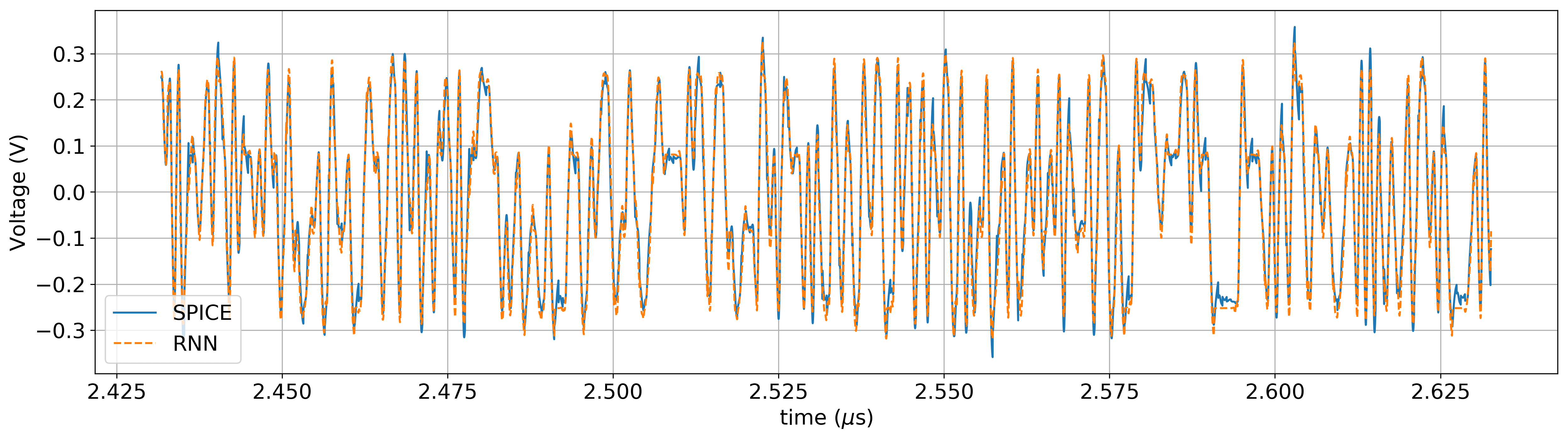
(c) After hundreds of thousands of bits

Figure 18: Waveform comparison between SPICE simulation and RNN prediction on PAM4 example with another PRBS

.

V Conclusion and Future work

In this paper, we propose using RNN for transient high-speed link simulation. It shows that using RNN-based model for circuit simulation is promising in terms of both the accuracy and the capability of improving computation efficiency. Through the proposed approach, an RNN model is trained and validated on a relatively short sequence generated from a circuit simulator. After the training completes, the RNN can be used to make predictions on the remaining sequence to generate an eye diagram. Using RNN model significantly enhances the computation efficiency because the transient waveforms are produced through inference, which saves iterations in solving nonlinear systems required by a circuit simulator. An RNN differs from a FNN by the fact that its parameters are shared across time. This is an advantage of an RNN because the number of tunable parameters is significantly reduced comparing to a FNN. However, it also becomes a challenge to train an RNN as the regular back-prop does not work anymore; instead, back-prop through time must be employed. Two topologies of the RNN, namely, ERNN and NARX-RNN, are investigated and compared in terms of the performance in high-speed link simulation. Through examples, it is demonstrated that ERNN without output feed-back is preferable in high-speed link simulation owing to its capability of batch learning and inference. It is also found out that LSTM network outperforms the vanilla RNN in terms of accuracy. We also investigates the impacts of training schemes and tunable parameters on both the accuracy and the generalization capability of an RNN model through examples.

Understanding the memory length of the data for training is important in achieving a balance between the computational cost and the accuracy of an RNN model. This remains an open problem in causal inference domain and the selection of a sufficient memory length to train an RNN model heavily relies on prior experience and substantial domain knowledge. One future work is to divide the full-channel modeling task into blocks where each block is represented by a standalone RNN model. Individual blocks can thus be swapped in and out to combine with different channel designs without retraining the RNN. Another future work is to take the equalization settings as inputs such that the RNN models can completely replace the transceivers circuit models.

References

- [1] N. Kapre and A. DeHon, “Parallelizing sparse matrix solve for SPICE circuit simulation using FPGAs,” in 2009 International Conference on Field-Programmable Technology, Dec 2009, pp. 190–198.
- [2] X. Chen, L. Ren, Y. Wang, and H. Yang, “GPU-Accelerated Sparse LU Factorization for Circuit Simulation with Performance Modeling,” IEEE Transactions on Parallel and Distributed Systems, vol. 26, no. 3, pp. 786–795, March 2015.
- [3] W. D. Guo, J. H. Lin, C. M. Lin, T. W. Huang, and R. B. Wu, “Fast methodology for determining eye diagram characteristics of lossy transmission lines,” IEEE Transactions on Advanced Packaging, vol. 32, no. 1, pp. 175–183, Feb 2009.
- [4] L. Zhu and N. Laptev, “Deep and confident prediction for time series at Uber,” in 2017 IEEE International Conference on Data Mining Workshops (ICDMW), vol. 00, Nov. 2018, pp. 103–110. [Online]. Available: doi.ieeecomputersociety.org/10.1109/ICDMW.2017.19
- [5] K. Cho, B. van Merrienboer, Ç. Gülçehre, F. Bougares, H. Schwenk, and Y. Bengio, “Learning phrase representations using RNN encoder-decoder for statistical machine translation,” CoRR, vol. abs/1406.1078, 2014. [Online]. Available: http://arxiv.org/abs/1406.1078
- [6] I. Sutskever, O. Vinyals, and Q. V. Le, “Sequence to sequence learning with neural networks,” in Proceedings of the 27th International Conference on Neural Information Processing Systems - Volume 2, ser. NIPS’14. Cambridge, MA, USA: MIT Press, 2014, pp. 3104–3112. [Online]. Available: http://dl.acm.org/citation.cfm?id=2969033.2969173
- [7] J. Ba, V. Mnih, and K. Kavukcuoglu, “Multiple object recognition with visual attention,” CoRR, vol. abs/1412.7755, 2014. [Online]. Available: http://arxiv.org/abs/1412.7755
- [8] A. Graves, “Generating sequences with recurrent neural networks,” CoRR, vol. abs/1308.0850, 2013. [Online]. Available: http://arxiv.org/abs/1308.0850
- [9] W. Liu, W. Na, L. Zhu, and Q. J. Zhang, “A review of neural network based techniques for nonlinear microwave device modeling,” in 2016 IEEE MTT-S International Conference on Numerical Electromagnetic and Multiphysics Modeling and Optimization (NEMO), July 2016, pp. 1–2.
- [10] A. Beg, P. W. C. Prasad, M. M. Arshad, and K. Hasnain, “Using recurrent neural networks for circuit complexity modeling,” in 2006 IEEE International Multitopic Conference, Dec 2006, pp. 194–197.
- [11] W.-T. Hsieh, C.-C. Shiue, and C. N. J. Liu, “A novel approach for high-level power modeling of sequential circuits using recurrent neural networks,” in 2005 IEEE International Symposium on Circuits and Systems, May 2005, pp. 3591–3594 Vol. 4.
- [12] Z. Chen, M. Raginsky, and E. Rosenbaum, “Verilog-A compatible recurrent neural network model for transient circuit simulation,” in 2017 IEEE 26th Conference on Electrical Performance of Electronic Packaging and Systems (EPEPS), Oct 2017, pp. 1–3.
- [13] T. Lu, J. Sun, K. Wu, and Z. Yang, “High-Speed Channel Modeling With Machine Learning Methods for Signal Integrity Analysis,” IEEE Transactions on Electromagnetic Compatibility, pp. 1–8, 2018.
- [14] N. Ambasana, G. Anand, D. Gope, and B. Mutnury, “S-Parameter and Frequency Identification Method for ANN-Based Eye-Height/Width Prediction,” IEEE Transactions on Components, Packaging and Manufacturing Technology, vol. 7, no. 5, pp. 698–709, May 2017.
- [15] C. Goay, P. Goh, N. Ahmad, and M. Ain, “Eye-height/width prediction using artificial neural networks from S-Parameters with vector fitting,” Journal of Engineering Science and Technology, vol. 13, no. 3, pp. 625–639, Mar. 2018.
- [16] G. Xue-lian, C. Zhen-nan, F. Nan, Z. Xiao-yu, and H. Jian-hong, “An artificial neural network model for S-parameter of microstrip line,” in 2013 Asia-Pacific Symposium on Electromagnetic Compatibility (APEMC), May 2013, pp. 1–4.
- [17] X. Zhang, Y. Cao, and Q. J. Zhang, “A combined transfer function and neural network method for modeling via in multilayer circuits,” in 2008 51st Midwest Symposium on Circuits and Systems, Aug 2008, pp. 73–76.
- [18] T. Nguyen and J. Schutt-Aine, “A Pseudo-supervised Machine Learning Approach to Broadband LTI Macro-Modeling,” in 2018 Joint Electromagnetic Compatibility (EMC) and Asia-Pacific Electromagnetic Compatibility (APEMC) Symposium, 2018.
- [19] F. Feng, C. Zhang, J. Ma, and Q. J. Zhang, “Parametric Modeling of EM Behavior of Microwave Components Using Combined Neural Networks and Pole-Residue-Based Transfer Functions,” IEEE Transactions on Microwave Theory and Techniques, vol. 64, no. 1, pp. 60–77, Jan. 2016.
- [20] X. Glorot, A. Bordes, and Y. Bengio, “Deep sparse rectifier neural networks,” in Proceedings of the Fourteenth International Conference on Artificial Intelligence and Statistics, ser. Proceedings of Machine Learning Research, G. Gordon, D. Dunson, and M. DudÃk, Eds., vol. 15. Fort Lauderdale, FL, USA: PMLR, 11–13 Apr 2011, pp. 315–323. [Online]. Available: http://proceedings.mlr.press/v15/glorot11a.html
- [21] D. P. Kingma and J. Ba, “Adam: A method for stochastic optimization,” CoRR, vol. abs/1412.6980, 2014. [Online]. Available: http://arxiv.org/abs/1412.6980
- [22] H. Robbins and S. Monro, “A Stochastic Approximation Method,” The Annals of Mathematical Statistics, vol. 22, no. 3, pp. 400–407, 1951.
- [23] T. Tieleman and G. Hinton, “Rmsprop gradient optimization,” URL http://www. cs. toronto. edu/tijmen/csc321/slides/lecture_slides_lec6. pdf, 2014.
- [24] J. L. Elman, “Finding structure in time,” COGNITIVE SCIENCE, vol. 14, no. 2, pp. 179–211, 1990.
- [25] R. Pascanu, T. Mikolov, and Y. Bengio, “Understanding the exploding gradient problem,” CoRR, vol. abs/1211.5063, 2012. [Online]. Available: http://arxiv.org/abs/1211.5063
- [26] R. J. Williams and J. Peng, “An Efficient Gradient-Based Algorithm for On-Line Training of Recurrent Network Trajectories,” Neural Computation, vol. 2, no. 4, pp. 490–501, Dec 1990.
- [27] I. Sutskever, “Training recurrent neural networks,” University of Toronto, Toronto, Ont., Canada, 2013. [Online]. Available: http://www.cs.utoronto.ca/~ilya/pubs/ilya_sutskever_phd_thesis.pdf
- [28] C. Olah. Understanding LSTM Networks. [Online]. Available: http://colah.github.io/posts/2015-08-Understanding-LSTMs/
- [29] K. Cho, B. van Merrienboer, Ç. Gülçehre, F. Bougares, H. Schwenk, and Y. Bengio, “Learning phrase representations using RNN encoder-decoder for statistical machine translation,” CoRR, vol. abs/1406.1078, 2014. [Online]. Available: http://arxiv.org/abs/1406.1078
- [30] S. Bengio, O. Vinyals, N. Jaitly, and N. Shazeer, “Scheduled Sampling for Sequence Prediction with Recurrent Neural Networks,” CoRR, vol. abs/1506.03099, 2015. [Online]. Available: http://arxiv.org/abs/1506.03099
- [31] Y. Cui, M. R. Ronchi, T.-Y. Lin, P. Dollr, and L. Zitnick, “Microsoft COCO captioning challenge,” 2015. [Online]. Available: http://cocodataset.org/#captions-challenge2015
- [32] A. Goyal, A. Lamb, Y. Zhang, S. Zhang, A. C. Courville, and Y. Bengio, “Professor Forcing: A New Algorithm for Training Recurrent Networks,” in Advances in Neural Information Processing Systems 29: Annual Conference on Neural Information Processing Systems 2016, December 5-10, 2016, Barcelona, Spain, 2016, pp. 4601–4609. [Online]. Available: http://papers.nips.cc/paper/6099-professor-forcing-a-new-algorithm-for-training-recurrent-networks
- [33] A. Vaswani, N. Shazeer, N. Parmar, J. Uszkoreit, L. Jones, A. N. Gomez, L. Kaiser, and I. Polosukhin, “Attention is all you need,” CoRR, vol. abs/1706.03762, 2017. [Online]. Available: http://arxiv.org/abs/1706.03762