Anisotropic pressure of deconfined QCD matter in presence of strong magnetic field within one-loop approximation

Abstract

Considering the general structure of the two point functions of quarks and gluons, we compute the free energy and pressure of a strongly magnetized hot and dense QCD matter created in heavy-ion collisions. In the presence of a strong magnetic field we found that the deconfined QCD matter exhibits a paramagnetic nature. One gets different pressures in directions parallel and perpendicular to the magnetic field due to the magnetization acquired by the system. We obtain both longitudinal and transverse pressures, and magnetization of hot deconfined QCD matter in the presence of the magnetic field. We have used hard thermal loop approximation for the heat bath. We obtained completely analytic expressions for pressure and magnetization under certain approximations. Various divergences appearing in free energy are regulated using appropriate counterterms. The obtained anisotropic pressure may be useful for a magnetohydrodynamics description of a hot and dense deconfined QCD matter produced in heavy-ion collisions.

I Introduction

Quantum chromodynamics (QCD) is the theory of the strong interaction that has two important features. One is the feeble interaction of quarks and gluons at high energy, and the other one is the confinement in which the interaction strength becomes strong at low energy. A transition between these two phases, namely confined to a deconfined state of hadronic matter known as quark-gluon plasma (QGP), is supposed to occur at around the energy scale or temperature $160$ MeV. In the early universe such a state of matter is presumed to be created after a few microseconds of big-bang. It can also exist in the core of neutron stars as matter density is much higher than the normal nuclear matter density. Various high energy heavy-ion experiments are underway in laboratories (LHC at CERN and RHIC at BNL) to study the formation of QGP and its properties for unraveling the characteristics of the QCD phase diagram. Future experiments are also planned in FAIR at GSI and NICA at Dubna to explore the high baryon density domain of the QCD phase diagram.

In recent years much attention has been paid in non-central heavy-ion collisions (HIC) where a magnetic field as high as $(10-30)m_{\pi}^{2}$ can be generated in a direction perpendicular to the reaction plane. This magnetic field is primarily created when the spectators recede from each other. This magnetic field strength, however, also decreases very fast to $(1-2)m_{\pi}^{2}$ after a timescale of $(4-5)$fm/c. The presence of an external magnetic field introduces an extra energy scale in the system in addition to the scales ($gT$ and $T$; $g$ is the strong coupling) associated with a heat bath. One can work with two limiting cases: the strong magnetic field limit $(eB>T^{2})$ and the weak magnetic field limit $(eB<T^{2})$. We note that the presence of an anisotropic magnetic field in the medium requires an appropriate modification of the present theoretical tools to investigate various properties of QGP. In recent years numerous activities have been in progress such as magnetic catalysis Alexandre:2000yf ; Gusynin:1997kj ; Lee:1997zj , inverse magnetic catalysis Bali:2011qj ; Bornyakov:2013eya ; Mueller:2015fka ; Ayala:2014iba ; Farias:2014eca ; Ayala:2014gwa ; Ayala:2016sln ; Ayala:2015bgv ; Mukherjee:2018ebw and chiral magnetic effect Kharzeev:2007jp ; Fukushima:2008xe ; Kharzeev:2009fn at finite temperature, and the chiral- and color-symmetry broken/restoration phase Avancini:2016fgq ; Fayazbakhsh:2010bh ; Fayazbakhsh:2010gc ; Andersen:2012zc ; Andersen:2014xxa . Also in progress is the study related to the equation of state (EoS) in thermal perturbative QCD (pQCD) models Bandyopadhyay:2017cle ; Rath:2017fdv , holographic models Rougemont:2015oea ; Finazzo:2016mhm and various thermodynamic properties Andersen:2012zc ; Andersen:2014xxa ; Strickland:2012vu ; Farias:2016gmy , refractive indices and decay constant of hadrons Fayazbakhsh:2012vr ; Fayazbakhsh:2013cha ; Bandyopadhyay:2016cpf ; Bandyopadhyay:2018gbw ; Chakraborty:2017vvg ; Islam:2018sog ; Ghosh:2018xhh ; Ghosh:2019fet ; soft photon production from conformal anomaly Basar:2012bp ; Ayala:2016lvs in HIC; modification of dispersion properties in a magnetized hot QED Sadooghi:2015hha ; Karmakar:2018aig and QCD Karmakar:2018aig ; Ayala:2018ina ; Das:2017vfh ; Hattori:2017xoo medium; and various transport coefficients Kurian:2018qwb ; Kurian:2018dbn ; Kurian:2017yxj , properties of quarkonia Singh:2017nfa ; Hasan:2018kvx , synchroton radiation Tuchin:2013prc2 , dilepton production from a hot magnetized QCD plasma Bandyopadhyay:2016fyd ; Tuchin:2013prc ; Tuchin:2013prc2 ; Tuchin:2013ie ; Sadooghi:2016jyf ; Bandyopadhyay:2017raf and in strongly coupled plasma in a strong magnetic field Mamo:2013efa .

The EoS is an important quantity and is of phenomenological importance for studying the hot and dense QCD matter, QGP, created in the relativistic heavy-ion collisions. This is because the EoS determines the thermodynamic properties of a hot and dense medium. Also the time evolution of the hot and dense fireball is studied through hydrodynamic models that require an EoS of the deconfined QCD matter as an input. In the absence of a magnetic field the EoS has systematically been computed in lattice QCD (LQCD) Gunther:2016vcp ; Bazavov:2017dus ; Bazavov:2017dsy and in hard thermal loop perturbation theory (HTLpt) within two loop [next-to-leading order (NLO)] Haque:2012my and three loop [next-to-NLO (NNLO)] 3loopglue1 ; 3loopglue2 ; 3loopqcd1 ; 3loopqcd2 ; 3loopqcd3 ; najmul3 ; Haque:2014rua at finite temperature and chemical potential. On the other hand as high magnetic fields are being produced in noncentral HIC, they subsequently decrease with the expansion of the fireball. Such systems, i.e. the expansion dynamics of a thermomagnetic medium, are governed by magnetohydrodynamics Inghirami:2016iru ; Roy:2017yvg that require a magnetic field dependent EoS as an input. In view of this, a systematic determination of EOS for a magnetized hot QCD medium is of great importance. Some LQCD effort has been made in Ref. Bali:2014kia that is limited to the temperature range (100-300)MeV. Recently we have computed Bandyopadhyay:2017cle the thermomagnetic EoS for the hot magnetized QCD medium within the weak magnetic field and HTL approximation. Also using HTL approximation, some thermodynamic quantities in lowest Landau level (LLL) within the strong field approximation has been numerically computed in Ref. Rath:2017fdv . However, for the gluonic case, this calculation assumes that the only effect of the magnetic field is to shift the Debye mass without any change in the general structure of two point functions at the finite temperature. It has explicitly been shown Karmakar:2018aig ; Ayala:2018ina ; Das:2017vfh ; Hattori:2017xoo that the presence of an external magnetic field breaks the rotational symmetry and the situation is quite different from what has been assumed in Ref. Rath:2017fdv . This seeks an improvement of the general structure of two point functions used in Ref. Rath:2017fdv .

In view of this we systematically compute the EoS within strong field approximation by exploiting the general structure of effective propagator of quarks and gluons in a thermomagnetic QCD medium. In the strong field limit, the magnetic field pushes higher Landau levels (HLL) to infinity compared to the lowest Landau level (LLL) Bandyopadhyay:2016fyd . Thus we work with the LLL approximation along with a scale hierarchy $eB>T^{2}>m_{f}^{2}$, where $m_{f}$ is the intrinsic mass scale associated with quarks. We also compute the magnetization which indicates that the deconfined hot and dense QCD matter is paramagnetic in nature. We further note that, in the presence of a strong magnetic field, we take into account the anisotropy between longitudinal and transverse pressures which is created due to the fact that the system acquires a magnetization along the field direction and is likely to elongate more along the direction of the magnetic field. We obtain a completely analytic expression for anisotropic (both longitudinal and transverse) pressures and magnetization under a certain approximation.

The paper has been organized as follows. In Sec. II we describe the basic setup for the computation of the free energy in this manuscript. In Sec. III we discuss the general structure of fermion self-energy in the presence of a strong magnetic field, the effective fermion propagator and associated form factors, and the quark free energy in one loop up to $\mathcal{O}(g^{4})$. The hard and soft contributions of gluon free energy up to $\mathcal{O}(g^{4})$ are also calculated in Sec. IV within one-loop HTL approximation. In Sec. V the pressure of an anisotropic system is discussed. We discuss our results in Sec. VI. Finally, we conclude in Sec. VII.

II Setup

The total thermodynamic free energy up to one-loop order in HTLpt in the presence of a background magnetic field, $B$, can be written as

$$F = F_{q}+F_{g}+F_{0}+\Delta{\mathcal{E}}^{0}_{T}+\Delta{\mathcal{E}}_{T}^{B}$$ (1)

where $F_{q}$ and $F_{g}$ are, respectively, the quark and gluon part of the free energy which will be computed in presence of magnetic field with an HTL approximation. $F_{0}$ is the tree level contribution due to the constant magnetic field, given as

$$F_{0}\rightarrow\frac{1}{2}B^{2}+\Delta{\mathcal{E}}_{0}^{B^{2}},$$ (2)

where $\Delta{\mathcal{E}}_{0}^{B^{2}}$ is a counterterm of ${\mathcal{O}}{[(q_{f}B)^{2}]}$ from vacuum as we will see later. The $\Delta{\mathcal{E}}_{T}$ is a counterterm independent of the magnetic field (viz. ${\mathcal{O}}[(q_{f}B)^{0}T^{4}]$ )as

$$\Delta{\mathcal{E}}^{0}_{T} = \Delta{\mathcal{E}}^{\mbox{\tiny{HTL}}}_{T}+\Delta{\mathcal{E}}_{T},$$ (3)

where $\Delta{\mathcal{E}}^{\mbox{\tiny{HTL}}}_{T}$ is the HTL counterterm najmul3 ; Haque:2014rua . The counterterm $\Delta{\mathcal{E}}_{T}$ arises due to the quark loop in the gluonic two point function in presence of magnetic field but the field dependence explicitly gets canceled from the denominator and numerator as we will see later. Finally, the counterterm $\Delta{\mathcal{E}}_{T}^{B}$ is of order ${\mathcal{O}}[(q_{f}B)T^{2}]$ and ${\mathcal{O}}[(q_{f}B)^{3}/T^{2}]$ .

The pressure of a system is defined as

$$P=-F.$$ (4)

We also note the QCD Casimir numbers are $C_{A}=N_{c}$, $d_{A}=N_{c}^{2}-1$, $d_{F}=N_{c}N_{f}$ and $C_{F}=(N_{c}^{2}-1)/2N_{c}$ where $N_{c}$ is the number of color and $N_{f}$ is the number of quark flavor.

III Quarks in a strong magnetic field

III.1 General structure of fermion self-energy in strong field approximation

It is established that the presence of a heat bath breaks the Lorentz(boost) invariance, whereas the presence of a magnetic field, $B$, breaks the rotational symmetry of the system. In such a situation one needs to construct a manifestly covariant structure of the self-energy. The presence of a heat bath introduces a four vector $u^{\mu}$, which is the velocity of the heat bath in addition to $P^{\mu}$, the four momentum of the external fermion. Now, in the case of noncentral heavy ion collisions, when QGP can be generally identified by the presence of external anisotropic magnetic and electric fields, the said heat bath is further considered to be in the vicinity of an external electromagnetic field. In this case one can construct two more four vectors in the comoving frame of the heat bath, i.e., $n^{\mu}$ and $e^{\mu}$, thereby characterizing the previously mentioned magnetic and electric fields, respectively. This is done by combining the electromagnetic field tensor $F^{\mu\nu}$ or its dual $\tilde{F}^{\mu\nu}$ with the fluid velocity $u^{\mu}$ as

$$n_{\mu}\equiv\frac{1}{2B}\epsilon_{\mu\nu\rho\lambda}\,u^{\nu}F^{\rho\lambda} = \frac{1}{B}u^{\nu}{\tilde{F}}_{\mu\nu}=(0,0,0,1),$$ (5)

$$e_{\mu} = \frac{1}{E}u^{\nu}F_{\mu\nu}=(0,1,0,0),$$ (6)

where the external magnetic and electric fields are considered to be in the $z$ and $x$ directions, respectively. This can further be justified by the structure of the electromagnetic field tensor

$$F^{\mu\nu}=\left({\begin{array}[]{cccc}0&E&0&0\\ -E&0&-B&0\\ 0&B&0&0\\ 0&0&0&0\\ \end{array}}\right)$$ (11)

which has been projected out along the four velocity, i.e. the rest frame of heat bath as $u^{\mu}=(1,0,0,0)$. This also uniquely establishes a connection between the heat bath, the external magnetic field along the $z$ direction and the external electric field along the $x$ direction. The general expression of $F^{\mu\nu}$ in terms of the four vectors $u^{\mu}$, $e^{\mu}$ and $n^{\mu}$ in the local rest frame of the heat bath is given by

$$F^{\mu\nu} = E\big{(}e^{\mu}u^{\nu}-e^{\nu}u^{\mu}\big{)}+B\epsilon^{\mu\nu\rho\lambda}u_{\rho}n_{\lambda}.$$ (12)

At this point we would also like to mention that in the rest part of our manuscript, following the ideal magnetohydrodynamics approximation we consider $e_{\mu}=0$, assuming the plasma in scrutiny has an infinite electrical conductivity Inghirami:2016iru .

The fermion self-energy $\Sigma(P)$ is $4\times 4$ matrix that can be constructed from Dirac $\gamma$ matrices. The self-energy will also depend on four vectors $P^{\mu}$, $u^{\mu}$ and $n^{\mu}$. In the presence of the magnetic field one can generally define

$$P_{\perp}^{\mu} = P^{\mu}-(P\cdot u)u^{\mu}+(P\cdot n)n^{\mu},$$ (13)

$$P_{\shortparallel}^{\mu} = (P\cdot u)u^{\mu}-(P\cdot n)n^{\mu},$$ (14)

$$p_{\perp}^{2} = (P^{\mu}u_{\mu})^{2}-(P^{\mu}n_{\mu})^{2}-P^{\mu}P_{\mu}$$ (15)

$$= p_{1}^{2}+p_{2}^{2}=-P_{\perp}^{2}.$$

As mentioned in the Introduction, in the present work we will be dealing with very strong external anisotropic magnetic fields, which are of relevance for initial stages of a noncentral heavy-ion collisions. In the presence of such strong magnetic fields ($q_{f}B\gg T^{2}$), we usually confine ourselves in the LLL. The reason for this assumption can be simply understood by looking at the dispersion relation in the presence of an external magnetic field along $z$ direction, i.e. $E_{n}=p_{0}=\sqrt{p_{3}^{2}+m_{f}^{2}+2neB}$, with $n$ representing the number of Landau levels. As can be seen from the above expression, for LLL, i.e. for $n=0$, the dispersion relation is independent of $eB$; hence a higher value of $eB$ does not affect it, instead pushing all other HLLs ($n\neq 0$) far away from LLL (see Fig.1 of Ref Bandyopadhyay:2016fyd ). So, for strong enough $eB$, the energy gap becomes too large for a fermion to hop out of LLL and realistically we can work only with LLL. In LLL with a strong field approximation ($q_{f}B\gg T^{2}$), an effective dimensional reduction takes place for fermions from (3+1) to (1+1) whereas gluons move in usual (3+1) dimension Gusynin:1995nb . In addition one has also a scale associated with the current quark mass $m_{f}$. In LLL the electrical conductivity is very sensitive to $m_{f}$ as it becomes infinite in the massless limit. This is because in the massless limit ($m_{f}=0$) due to chirality conservation the scattering processes are forbidden such that the electrical conductivity diverges without scattering Hattori:2016cnt . We will also see below in Eq. (74) that the gluons acquire a screening mass $m_{D}^{s}\sim g\sqrt{q_{f}B}$ ($g$ is the QCD coupling). Since we are interested in finite temperature effect, we can consider $T\gg m_{D}^{s},m_{f}$. In this paper we will work in the following hierarchy $q_{f}B\gg T^{2}\gg(m_{D}^{s})^{2},m_{f}^{2}$.

In the LLL the transverse component of the momentum, $P_{\perp}=0$. Thus, $P^{\mu}$ reduces to $P_{\shortparallel}^{\mu}$. $P_{\shortparallel}^{\mu}$ can be written as a linear combination of $u^{\mu}$ and $n^{\mu}$. In the chiral limit the general structure of fermion self-energy in lowest Landau level can be written as

$$\Sigma(p_{0},p_{3}) = a/\!\!\!u+b/\!\!\!n+c\gamma_{5}/\!\!\!u+d\gamma_{5}/\!\!\!n,$$ (16)

where $/\!\!\!{u}=\gamma_{0}$ and $/\!\!\!{n}=\gamma^{3}n_{3}=\gamma^{3}$. Now, the various form factors can be obtained as

$$a = \frac{1}{4}\operatorname{\text{Tr}}[\Sigma/\!\!\!u],$$ (17)

$$b = -\frac{1}{4}\operatorname{\text{Tr}}[\Sigma/\!\!\!n],$$ (18)

$$c = \frac{1}{4}\operatorname{\text{Tr}}[\gamma_{5}\Sigma/\!\!\!u],$$ (19)

$$d = -\frac{1}{4}\operatorname{\text{Tr}}[\gamma_{5}\Sigma/\!\!\!n].$$ (20)

Finally, using the chirality projectors we can express the general structure of the fermion self-energy as,

$$\Sigma(P)=\mathcal{P}_{R}\ /\!\!\!\!{A}\ \mathcal{P}_{L}+\mathcal{P}_{L}\ /\!\!\!\!{B}\ \mathcal{P}_{R},$$ (21)

where

$$/\!\!\!\!{A}=(a+c)/\!\!\!{u}+(b+d)/\!\!\!{n},$$ (22)

$$/\!\!\!\!{B}=(a-c)/\!\!\!{u}+(b-d)/\!\!\!{n},$$ (23)

$$\mathcal{P}_{R}=\frac{1}{2}(\mathbbm{1}+\gamma_{5}),$$ (24)

$$\mathcal{P}_{L}=\frac{1}{2}(\mathbbm{1}-\gamma_{5}).$$ (25)

III.2 One loop quark self-energy in presence of a strong magnetic field

Using the modified fermion propagator in strong field approximation, one can right away write down the quark self-energy in Feynman gauge from Fig. 1 as

$$\Sigma(P) = -ig^{2}C_{F}\int\frac{d^{4}K}{(2\pi)^{4}}\gamma_{\mu}S(K)\gamma^{\mu}\Delta(K-P),$$ (26)

where the unmodified gluonic propagator is given as

$$\Delta(K-P)=\frac{1}{(k_{0}-p_{0})^{2}-(k-p)^{2}}=\frac{1}{(K-P)_{\shortparallel}^{2}-(k-p)_{\perp}^{2}}.$$ (27)

and the modified fermion propagator in LLL is given by

$$iS(K)=ie^{-{k_{\perp}^{2}}/{q_{f}B}}~{}~{}\frac{/\!\!\!\!{K}_{\shortparallel}+m_{f}}{K_{\shortparallel}^{2}-m_{f}^{2}}\left(\mathbbm{1}-i\gamma_{1}\gamma_{2}\right).$$ (28)

Figure 1: Self-energy diagram for a quark in a strong magnetic field approximation. The double line indicates the modified quark propagator in presence of strong magnetic field.

Now, the thermo-magnetic self-energy $\Sigma(P)$ can be written from Eq. (26) as

$$\Sigma(P) = -ig^{2}C_{F}\int\frac{d^{4}K}{(2\pi)^{4}}e^{-k_{\perp}^{2}/q_{f}B}\gamma_{\mu}\frac{(/\!\!\!\!{K}_{\shortparallel}+m_{f})}{(K_{\shortparallel}^{2}-m_{f}^{2})}\left(\mathbbm{1}-i\gamma_{1}\gamma_{2}\right)\gamma^{\mu}\Delta(K-P)$$ (29)

$$= -ig^{2}C_{F}\int\frac{d^{4}K}{(2\pi)^{4}}e^{-k_{\perp}^{2}/q_{f}B}\gamma_{\mu}/\!\!\!\!{K}_{\shortparallel}\left(\mathbbm{1}-i\gamma_{1}\gamma_{2}\right)\gamma^{\mu}\tilde{\Delta}_{\shortparallel}(K)\Delta(K-P)$$

$$= -2g^{2}C_{F}\sum\!\!\!\!\!\!\!\!\!\!\int\limits_{\{K\}}e^{-k_{\perp}^{2}/q_{f}B}\left[\left(\mathbbm{1}+i\gamma_{1}\gamma_{2}\right)/\!\!\!\!{K}_{\shortparallel}\right]\tilde{\Delta}_{\shortparallel}(K)\Delta(K-P),$$

where

$$\tilde{\Delta}_{\shortparallel}(K)=\frac{1}{k_{0}^{2}-k_{3}^{2}}$$ (30)

Also at finite temperature, the loop integration measure is replaced by

$$\int\frac{d^{4}K}{(2\pi)^{4}}\longrightarrow iT\sum\limits_{\{k_{0}\}}\int\frac{d^{3}k}{(2\pi)^{3}}\ \longrightarrow iT\sum\limits_{\{k_{0}\}}\int\frac{dk_{3}}{2\pi}\int\frac{d^{2}k_{\perp}}{(2\pi)^{2}}\hskip 5.69046pt.$$ (31)

Now the expressions of form factors for a particular flavor $f$ become

$$a=\frac{1}{4}\operatorname{\text{Tr}}[\Sigma\,/\!\!\!\!{u}] = -\frac{2g^{2}C_{F}}{4}\sum\!\!\!\!\!\!\!\!\!\!\int\limits_{\{K\}}e^{-\frac{k_{\perp}^{2}}{q_{f}B}}\operatorname{\text{Tr}}\bigg{[}(\mathbbm{1}+i\gamma_{1}\gamma_{2})\,/\!\!\!\!{k}_{\shortparallel}\,/\!\!\!\!{u}\bigg{]}\tilde{\Delta}_{\shortparallel}(K)\Delta(K-P)$$ (32)

$$= -2g^{2}C_{F}\sum\!\!\!\!\!\!\!\!\!\!\int\limits_{\{K\}}e^{-\frac{k_{\perp}^{2}}{q_{f}B}}k^{0}\tilde{\Delta}_{\shortparallel}(K)\Delta(K-P),$$

$$b=-\frac{1}{4}\operatorname{\text{Tr}}[\Sigma\>/\!\!\!\!{n}] = \frac{2g^{2}C_{F}}{4}\sum\!\!\!\!\!\!\!\!\!\!\int\limits_{\{K\}}e^{-\frac{k_{\perp}^{2}}{q_{f}B}}\operatorname{\text{Tr}}\bigg{[}\left(\mathbbm{1}+i\gamma_{1}\gamma_{2}\right)\,/\!\!\!\!{k}_{\shortparallel}\,/\!\!\!\!{n}\bigg{]}\tilde{\Delta}_{\shortparallel}(K)\Delta(K-P)$$ (33)

$$= 2g^{2}C_{F}\sum\!\!\!\!\!\!\!\!\!\!\int\limits_{\{K\}}e^{-\frac{k_{\perp}^{2}}{q_{f}B}}k^{3}\tilde{\Delta}_{\shortparallel}(K)\Delta(K-P),$$

$$c=\frac{1}{4}\operatorname{\text{Tr}}[\gamma_{5}\Sigma\,/\!\!\!\!{u}] = -\frac{2g^{2}C_{F}}{4}\sum\!\!\!\!\!\!\!\!\!\!\int\limits_{\{K\}}e^{-\frac{k_{\perp}^{2}}{q_{f}B}}\operatorname{\text{Tr}}\bigg{[}\gamma_{5}\left(\mathbbm{1}+i\gamma_{1}\gamma_{2}\right)\,/\!\!\!\!{k}_{\shortparallel}\,/\!\!\!\!{u}\bigg{]}\tilde{\Delta}_{\shortparallel}(K)\Delta(K-P)$$ (34)

$$= -2g^{2}C_{F}\sum\!\!\!\!\!\!\!\!\!\!\int\limits_{\{K\}}e^{-\frac{k_{\perp}^{2}}{q_{f}B}}k^{3}\tilde{\Delta}_{\shortparallel}(K)\Delta(K-P),$$

$$d=-\frac{1}{4}\operatorname{\text{Tr}}[\gamma_{5}\Sigma\,/\!\!\!\!{n}] = \frac{2g^{2}C_{F}}{4}\sum\!\!\!\!\!\!\!\!\!\!\int\limits_{\{K\}}e^{-\frac{k_{\perp}^{2}}{q_{f}B}}\operatorname{\text{Tr}}\bigg{[}\gamma_{5}(\mathbbm{1}+i\gamma_{1}\gamma_{2})\,/\!\!\!\!{k}_{\shortparallel}\,/\!\!\!\!{n}\bigg{]}\tilde{\Delta}_{\shortparallel}(K)\Delta(K-P)$$ (35)

$$= 2g^{2}C_{F}\sum\!\!\!\!\!\!\!\!\!\!\int\limits_{\{K\}}e^{-\frac{k_{\perp}^{2}}{q_{f}B}}k^{0}\tilde{\Delta}_{\shortparallel}(K)\Delta(K-P).$$

From the above four expressions it can be noted that $b=-c$ and $d=-a$. These form factors will be calculated in Appendix A.

III.3 Effective propagator and dispersion relation

The transverse momentum of the fermion becomes zero, i.e., $P_{\perp}=0$, in LLL. Thus the effective fermion propagator can be written using the Dyson-Schwinger equation as

$$S_{\text{eff}}(P_{\shortparallel})=\frac{1}{/\!\!\!\!{P_{\shortparallel}}+\Sigma}.$$ (36)

Subsequently the inverse fermion propagator can be written as

$$S^{-1}_{\text{eff}}(P) ={/\!\!\!\!{P_{\shortparallel}}+\Sigma}$$ (37)

$$=\mathcal{P}_{R}/\!\!\!\!{L}\mathcal{P}_{L}+\mathcal{P}_{L}/\!\!\!\!{R}\mathcal{P}_{R},$$ (38)

where

$$/\!\!\!\!{L}=/\!\!\!\!{P}+(a+c)/\!\!\!{u}+(b+d)/\!\!\!{n},$$ (39)

$$/\!\!\!\!{R}=/\!\!\!\!{P}+(a-c)/\!\!\!{u}+(b-d)/\!\!\!{n}.$$ (40)

Now the effective propagator can be written as

$${S}_{\text{eff}}(P_{\shortparallel})=\mathcal{P}_{R}\frac{/\!\!\!\!{R}}{R^{2}}\mathcal{P}_{L}+\mathcal{P}_{L}\frac{/\!\!\!\!{L}}{L^{2}}\mathcal{P}_{R}.$$ (41)

We have

$$L^{2}=(p_{0}+(a+c))^{2}-\big{(}p_{3}-(b+d)\big{)}^{2},$$ (42)

$$R^{2}=(p_{0}+(a-c))^{2}-\big{(}p_{3}-(b-d)\big{)}^{2}.$$ (43)

Now putting $a=-d$ and $b=-c$, one gets

$$L^{2}=p_{0}^{2}-p_{3}^{2}+2(a-b)(p_{0}-p_{3})=(p_{0}-p_{3})(p_{0}+p_{3}+2(a-b)),$$ (44)

$$R^{2}=p_{0}^{2}-p_{3}^{2}+2(a+b)(p_{0}+p_{3})=(p_{0}+p_{3})(p_{0}-p_{3}+2(a+b)).$$ (45)

Various discrete symmetries of the effective two-point functions are discussed in detail in Ref. Das:2017vfh . The form factors are calculated in Appendix A and given as

$$a=-d=-\frac{g^{2}C_{F}}{4\pi^{2}}\bigg{[}\sum_{f}q_{f}B\frac{p_{0}}{p_{0}^{2}-p_{3}^{2}}\ln 2-\sum_{f}\left(q_{f}B\right)^{2}\frac{\zeta^{\prime}(-2)}{2T^{2}}\frac{p_{0}(p_{0}^{2}+p_{3}^{2})}{(p_{0}^{2}-p_{3}^{2})^{2}}\bigg{]},$$ (46)

$$b = -c=\frac{g^{2}C_{F}}{4\pi^{2}}\bigg{[}\sum_{f}q_{f}B\frac{p_{3}}{p_{0}^{2}-p_{3}^{2}}\ln 2-\sum_{f}q_{f}B\frac{p_{3}}{2T^{2}}\zeta^{\prime}(-2)$$ (47)

$$-\sum_{f}\left(q_{f}B\right)^{2}\frac{\zeta^{\prime}(-2)}{T^{2}}\frac{p_{0}^{2}p_{3}}{(p_{0}^{2}-p_{3}^{2})^{2}}\bigg{]}.$$

The magnetic mass is found by taking the dynamic limit of $R^{2}$ and $L^{2}$ in Eq. (41), i.e., $R^{2}|_{p\rightarrow 0,p_{0}=0}=L^{2}|_{p\rightarrow 0,p_{0}=0},$ and is given by

$$M_{\text{sfa}}^{2}=\frac{g^{2}C_{F}}{4\pi^{2}T^{2}}\left(\sum_{f}(q_{f}B)~{}T^{2}\ln{4}-\sum_{f}\left(q_{f}B\right)^{2}\zeta^{\prime}(-2)\right).$$ (48)

One can notice that the magnetic mass is dependent on both magnetic field and temperature.

Now we discuss the dispersion properties of fermions in a hot magnetized medium. The dispersion curves are obtained by solving, $L^{2}=0$ and $R^{2}=0$ given in Eq. (41), numerically. There are four modes, two come from $L^{2}=0$ and two from $R^{2}=0$. In LLL only two modes are allowed Das:2017vfh : one $L$ mode with energy $\omega_{L}$ of a positively charged fermion having spin up and another one from $R$ mode with energy $\omega_{R}$ of a negatively charged fermion having spin-down. These two modes are plotted in Fig. 2. In the LLL aproximation the transverse momentum of fermion becomes zero. Thus the dynamics of the system becomes two dimensional. At high $p_{z}$ both the modes of dispersion resembles the free dispersion mode. We also note that the reflection symmetry is broken in the presence of a magnetic field Das:2017vfh .

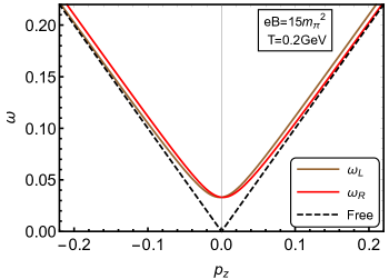
Figure 2: Dispersion relation of the fermion in the presence of a strong magnetic field

III.4 One-loop quark free energy in the presence of a strongly magnetized medium

The quark free energy can be written as

$$F_{q}=-d_{F}\sum\!\!\!\!\!\!\!\!\!\!\int\limits_{\{p_{0}\}}~{}\frac{d^{3}p}{(2\pi)^{3}}\ln{\left(\det[S^{-1}_{\text{eff}}(p_{0},p_{3})]\right)}.$$ (49)

Effective fermion self-energy can be written as

$$S^{-1}_{\text{eff}}=/\!\!\!\!{P_{\shortparallel}}+\Sigma = (p_{0}+a)/\!\!\!{u}+(b-p_{3})/\!\!\!{n}+c\gamma_{5}/\!\!\!{u}+d\gamma_{5}/\!\!\!{n}$$ (50)

$$= (p_{0}+a)\gamma^{0}+(b-p_{3})\gamma^{3}+c\gamma_{5}\gamma^{0}+d\gamma_{5}\gamma^{3}.$$

Now we evaluate the determinant as

$$\det[S^{-1}_{\text{eff}}] = \bigg{(}(b+c-p_{3})^{2}-(a+d+p_{0})^{2}\bigg{)}\bigg{(}(-b+c+p_{3})^{2}-(a-d+p_{0})^{2}\bigg{)}$$ (51)

$$= (p_{0}^{2}-p_{3}^{2})\bigg{(}(p_{0}+2a)^{2}-(p_{3}-2b)^{2}\bigg{)}$$

$$= P_{\shortparallel}^{2}\left(P_{\shortparallel}^{2}+4ap_{0}+4bp_{3}+4a^{2}-4b^{2}\right)$$

$$= P_{\shortparallel}^{4}\left(1+\frac{4a^{2}-4b^{2}+4ap_{0}+4bp_{3}}{P_{\shortparallel}^{2}}\right),$$

where we have used $d=-a$ and $c=-b$.

So Eq. (49) becomes

$$F_{q} = -d_{F}\sum\!\!\!\!\!\!\!\!\!\!\int\limits_{\{p_{0}\}}~{}\frac{d^{3}p}{(2\pi)^{3}}\ln\bigg{[}P_{\shortparallel}^{4}\left(1+\frac{4a^{2}-4b^{2}+4ap_{0}+4bp_{3}}{P_{\shortparallel}^{2}}\right)\bigg{]}$$ (52)

$$= -2d_{F}\sum\!\!\!\!\!\!\!\!\!\!\int\limits_{\{p_{0}\}}~{}\frac{d^{3}p}{(2\pi)^{3}}\ln{(-P_{\shortparallel}^{2})}-d_{F}\sum\!\!\!\!\!\!\!\!\!\!\int\limits_{\{p_{0}\}}~{}\frac{d^{3}p}{(2\pi)^{3}}\ln\bigg{[}1+\frac{4a^{2}-4b^{2}+4ap_{0}+4bp_{3}}{P_{\shortparallel}^{2}}\bigg{]}$$

$$= F^{\text{ideal}}_{q}+F^{\prime}_{q},$$

where the free energy of free quarks Strickland:2012vu

$$F^{\text{ideal}}_{q} = -2d_{F}\sum\!\!\!\!\!\!\!\!\!\!\int\limits_{\{p_{0}\}}~{}\frac{d^{3}p}{(2\pi)^{3}}\ln{(-P_{\shortparallel}^{2})}=-2d_{F}\sum_{f}\frac{q_{f}B}{(2\pi)^{2}}\sum\!\!\!\!\!\!\!\!\!\!\int\limits_{\{p_{0}\}}dp_{3}\ln{(-P_{\shortparallel}^{2})}$$ (53)

$$= -d_{F}\sum_{f}\frac{q_{f}BT^{2}}{12},$$

and

$$F^{\prime}_{q} = -d_{F}\sum\!\!\!\!\!\!\!\!\!\!\int\limits_{\{p_{0}\}}~{}\frac{d^{3}p}{(2\pi)^{3}}\ln\bigg{[}1+\frac{4a^{2}-4b^{2}+4ap_{0}+4bp_{3}}{P_{\shortparallel}^{2}}\bigg{]}$$ (54)

$$= -d_{F}\sum\!\!\!\!\!\!\!\!\!\!\int\limits_{\{p_{0}\}}~{}\frac{d^{3}p}{(2\pi)^{3}}\bigg{[}\frac{4\left(ap_{0}+bp_{3}\right)}{P_{\shortparallel}^{2}}+\frac{4\left(a^{2}P^{2}-b^{2}P^{2}-2a^{2}p_{0}^{2}-2b^{2}p_{3}^{2}-4abp_{0}p_{3}\right)}{P_{\shortparallel}^{4}}$$

$$\hskip 113.81102pt+\mathcal{O}(g^{6})\bigg{]},$$

where we have kept terms up to $\mathcal{O}(g^{4})$ to obtain the analytic exprssion of free energy. The expansion made above is valid for $g^{2}(q_{f}B/T^{2})<1$, which can be realized as $(q_{f}B)/T^{2}\gtrsim 1$ and $g\ll 1$.

As in the strong field approximation, the fermion is considered to be in LLL. So Eq. (54) becomes,

$$F^{\prime}_{q} = -d_{F}\sum_{f}\frac{q_{f}B}{(2\pi)^{2}}\sum\!\!\!\!\!\!\!\!\!\!\int\limits_{\{p_{0}\}}~{}dp_{3}~{}\bigg{[}\frac{4\left(ap_{0}+bp_{3}\right)}{P_{\shortparallel}^{2}}+\frac{4\left(a^{2}P^{2}-b^{2}P^{2}-2a^{2}p_{0}^{2}-2b^{2}p_{3}^{2}-4abp_{0}p_{3}\right)}{P_{\shortparallel}^{4}}$$ (55)

$$\hskip 128.0374pt+\mathcal{O}(g^{6})\bigg{]}.$$

The sum-integrals are calculated in Appendix (B), and the expression for the quark free energy up to $\mathcal{O}(g^{4})$ is given by

$$F_{q} = -d_{F}\sum_{f}\frac{q_{f}BT^{2}}{12}-4d_{F}\sum_{f}\frac{\left(q_{f}B\right)^{2}}{(2\pi)^{2}}\frac{g^{2}C_{F}}{4\pi^{2}}\left(\frac{\Lambda}{4\pi T}\right)^{2\epsilon}\Bigg{[}\frac{1}{8\epsilon}\left(4\ln{2}-q_{f}B\frac{\zeta^{{}^{\prime}}(-2)}{T^{2}}\right)$$ (56)

$$+\frac{1}{24576}\Bigg{\{}12288\ln{2}(3\gamma_{E}+4\ln{2}-\ln{\pi})+\frac{256\zeta[3]}{\pi^{4}T^{2}}\Big{(}2\pi^{4}T^{2}-3g^{2}C_{F}(q_{f}B)\ln{2}$$

$$+3\pi^{2}(q_{f}B)(2+3\gamma_{E}+4\ln{2}-\ln{\pi})\Big{)}-\frac{8g^{2}C_{F}}{\pi^{6}T^{4}}(q_{F}B)^{2}\zeta[3]^{2}(4+105\ln{2})$$

$$+\frac{7245g^{2}C_{F}}{\pi^{8}T^{6}}(q_{F}B)^{3}\zeta[3]^{3}\Bigg{\}}\Bigg{]}$$

$$= -d_{F}\sum_{f}\frac{q_{f}BT^{2}}{12}-4d_{F}\sum_{f}\frac{\left(q_{f}B\right)^{2}}{(2\pi)^{2}}\frac{g^{2}C_{F}}{4\pi^{2}}\Bigg{[}\frac{1}{8\epsilon}\left(4\ln{2}-q_{f}B\frac{\zeta^{{}^{\prime}}(-2)}{T^{2}}\right)+\frac{1}{24576}$$

$$\Bigg{\{}12288\ln 2\left(3\gamma_{E}+2\ln\hat{\Lambda}+\ln 4-\ln\pi\right)+\frac{256\zeta[3]}{\pi^{4}T^{2}}\bigg{(}-3C_{F}g^{2}q_{f}B\ln 2$$

$$+6\pi^{2}q_{f}B\ln\hat{\Lambda}+3\pi^{2}q_{f}B(2+3\gamma_{E}+\ln 4-\ln\pi)+2\pi^{4}T^{2}\bigg{)}-\frac{8g^{2}C_{F}}{\pi^{6}T^{4}}(q_{f}B)^{2}$$

$$\times\zeta[3]^{2}(4+105\ln{2})+\frac{7245g^{2}C_{F}}{\pi^{8}T^{6}}(q_{f}B)^{3}\zeta[3]^{3}\Bigg{\}}\Bigg{]},$$

where $\hat{\Lambda}=\Lambda/2\pi T$. The quark free energy has ${\mathcal{O}}[\left(q_{f}B\right)^{2}/\epsilon]$ and ${\mathcal{O}}[\left(q_{f}B\right)^{3}/T^{2}\epsilon]$ divergences.

IV Gluons in a strong magnetic field

IV.1 General structure of gauge boson free energy

The partition function for a gluon can generally be written in Euclidean space Bandyopadhyay:2017cle as

$${\mathcal{Z}}_{g}={\cal Z}{\cal Z}^{\textrm{ghost}},~{}~{}{\mathcal{Z}}=N_{\xi}\prod_{n,\bm{p}}\sqrt{\frac{(2\pi)^{D}}{\det D_{\mu\nu,E}^{-1}}},~{}~{}{\mathcal{Z}}^{\textrm{ghost}}=\prod_{n,\bm{p}}P_{E}^{2},$$ (57)

where the product over $\bm{p}$ is for the spatial momentum whereas that over $n$ is for the discrete bosonic Matsubara frequencies ($\omega_{n}=2\pi n\beta;\,\,n=0,1,2,\cdots$) due to Euclidean time, $D$ is the spacetime dimension of the theory. $D_{\mu\nu,E}^{-1}$ is the inverse gauge boson propagator in Euclidean space with $P_{E}^{2}=\omega_{n}^{2}+p^{2}$ the square of four momentum. $N_{\xi}=1/(2\pi\xi)^{D/2}$ is the normalization that originates from the introduction of a Gaussian integral at each location of position while averaging over the gauge condition function with a width $\xi$, the gauge fixing parameter. Gluon free energy can now be written Bandyopadhyay:2017cle as

$$F_{g}=-d_{A}\frac{T}{V}\ln{\cal Z}_{g}=d_{A}\left[\frac{1}{2}\sum\!\!\!\!\!\!\!\!\!\int\limits_{P_{E}}~{}\ln\Big{[}\textsf{det}\left(D_{\mu\nu,E}^{-1}(P_{E})\right)\Big{]}-\sum\!\!\!\!\!\!\!\!\!\int\limits_{P_{E}}~{}\ln P_{E}^{2}\right].$$ (58)

We note that the presence of the normalization factor $N_{\xi}$ eliminates the gauge dependence explicitly.

For an ideal case $\textsf{det}\left(D_{\mu\nu,E}^{-1}(P)\right)=(P_{E}^{2})^{4}/\xi$, and hence the free energy for $d_{A}$ massless spin one gluons yields as

$$F_{g}^{\textrm{ideal}}=d_{A}\sum\!\!\!\!\!\!\!\!\!\int\limits_{P_{E}}~{}\ln P_{E}^{2}=d_{A}\sum\!\!\!\!\!\!\!\!\!\int\limits_{P}~{}\ln\left(-P^{2}\right)=-d_{A}\frac{\pi^{2}T^{4}}{45},$$ (59)

where $P$ is four-momentum in Minkowski space and can be written as $P^{2}=p_{0}^{2}-p^{2}.$

In the presence of thermal background medium Lebellac;1996 ; Kapusta:1989tk ; Karmakar:2018aig one can have

$$\textsf{det}\left(D_{\mu\nu,E}^{-1}(P_{E})\right)=\frac{P_{E}^{2}}{\xi}\left(P_{E}^{2}+\Pi_{T}\right)^{2}\left(P_{E}^{2}+\Pi_{L}\right),$$ (60)

which has four eigenvalues. Those are, respectively, $P_{E}^{2}/\xi$, $(P_{E}^{2}+\Pi_{L})$, and twofold degenerate $(P_{E}^{2}+\Pi_{T})$ where $\Pi_{T}$ and $\Pi_{L}$, respectively, are the transverse and longitudinal part of the gluon self-energy in a heat bath. Also we considered $D=4$, and the spatial dimension, $d=3$ throughout this manuscript. From now on, we use Minkowski momentum $P$. Eventually the free energy becomes Bandyopadhyay:2017cle

$$F_{g}^{\textrm{th}} = \frac{1}{2}\left[\sum\!\!\!\!\!\!\!\!\!\int\limits_{P}~{}\ln\left(-P^{2}\right)+2\sum\!\!\!\!\!\!\!\!\!\int\limits_{P}~{}\ln\left(-P^{2}+\Pi_{T}\right)+\sum\!\!\!\!\!\!\!\!\!\int\limits_{P}~{}\ln\left(-P^{2}+\Pi_{L}\right)\right]-\sum\!\!\!\!\!\!\!\!\!\int\limits_{P}~{}\ln\left(-P^{2}\right),$$ (61)

$$= \sum\!\!\!\!\!\!\!\!\!\int\limits_{P}~{}\ln\left(-P^{2}+\Pi_{T}\right)+\frac{1}{2}\sum\!\!\!\!\!\!\!\!\!\int\limits_{P}~{}\ln\left(1-\frac{\Pi_{L}}{P^{2}}\right)$$

$$= d_{A}\left[(d-1)F_{g}^{T}+F_{g}^{L}\right],$$ (62)

Also, $F_{g}^{L}$ and $F_{g}^{T}$ are, respectively, the longitudinal and transverse part of the gluon free energy. Using general structure of two-0point functions of the gauge boson, both of them are evaluated in Refs. Lebellac;1996 ; Kapusta:1989tk ; Karmakar:2018aig .

Now, the general structure of the inverse propagator of a gauge boson in ther presence of a hot magnetized medium is computed in Ref. Karmakar:2018aig as

$$\left(\mathcal{D}_{\mu\nu}\right)^{-1}=\frac{P^{2}}{\xi}\eta_{\mu\nu}+\left(P_{m}^{2}-b\right)B_{\mu\nu}+\left(P_{m}^{2}-c\right)R_{\mu\nu}+\left(P_{m}^{2}-d\right)Q_{\mu\nu},$$ (63)

where

$$P_{m}^{2}=P^{2}\frac{\xi-1}{\xi}$$ (64)

and $b$, $c$, $d$ are the form factors corresponding to the three projection tensors $B^{\mu\nu}$,$R^{\mu\nu}$ and $Q^{\mu\nu}$, respectively for gauge boson self-energy Karmakar:2018aig . The determinant of the inverse of the gauge boson propagator can be evaluated from Eq. (63) as

$$\textsf{det}\left(D_{\mu\nu,E}^{-1}(P)\right)=-\frac{P^{2}}{\xi}\left(-P^{2}+b\right)\left(-P^{2}+c\right)\left(-P^{2}+d\right),$$ (65)

which has four eigenvalues: $-P^{2}/\xi,\,\left(-P^{2}+b\right),\,\left(-P^{2}+c\right),\,{\mbox{and}}\,\left(-P^{2}+d\right)$. We note here that one has two distinct transverse modes coming from $(-P^{2}+c)=0$ and $(-P^{2}+d)=0$ respectively, in a thermomagnetic medium instead of a two fold degenerate transverse mode $(-P^{2}+\Pi_{T})=0$ in thermal medium in Eq. (60).

Using Eq. (65) in Eq. (58), the one-loop gluon free energy for hot magnetized medium is given Karmakar:2018aig by

$$F_{g}=d_{A}\left[\mathcal{F}_{g}^{1}+\mathcal{F}_{g}^{2}+\mathcal{F}_{g}^{3}\right],$$ (66)

where

$$\mathcal{F}_{g}^{1} =\frac{1}{2}\sum\!\!\!\!\!\!\!\!\!\int\limits_{P}~{}\ln\left(1-\frac{b}{P^{2}}\right),$$ (67a)

$$\mathcal{F}_{g}^{2} =\frac{1}{2}\sum\!\!\!\!\!\!\!\!\!\int\limits_{P}~{}\ln\left(-P^{2}+c\right),$$ (67b)

$$\mathcal{F}_{g}^{3} =\frac{1}{2}\sum\!\!\!\!\!\!\!\!\!\int\limits_{P}~{}\ln\left(-P^{2}+d\right).$$ (67c)

The various structure functions are obtained in Ref. Karmakar:2018aig in both strong and weak field approximation. In the following sections we obtain the gluon free energy in strong field approximation.

IV.2 Gluon free energy in a strongly magnetized hot and dense medium

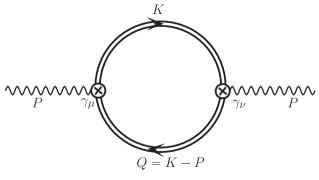
Figure 3: Self-energy diagram for a gluon in the strong magnetic field approximation. The double line indicates the modified quark propagator in the presence of a strong magnetic field.

Within the strong field approximation ($m_{f}^{2}<T^{2}<q_{f}B$) the expressions for the different contributions of the gluon free energy in LLL can now be obtained from Eqs. (66). Combining Eqs. (67a), (67b), and (67c) with Eq. (66), the total one-loop free energy expanded up to ${\mathcal{O}}[g^{4}]$ is given by

$$F_{g} \approx d_{A}\left[\sum\!\!\!\!\!\!\!\!\!\int\limits_{P}~{}\ln\left(-P^{2}\right)-\frac{b+c+d}{2P^{2}}-\frac{b^{2}+c^{2}+d^{2}}{4P^{4}}\right],$$ (68)

where the expansion is made to obtain analytical expression for free energy which is valid for $g^{2}(q_{f}B/T^{2})<1$, and it can be realized as $(q_{f}B)/T^{2}\gtrsim 1$ and $g\ll 1$.

Now the various structure functions involved therein are obtained in Ref. Karmakar:2018aig . For simplicity we consider $m_{f}=0$ with a hierarchy of scales as $m_{f}^{2}\sim m^{2}_{\textrm{th}}\sim g^{2}T^{2}<T^{2}<q_{f}B$ and write down those structure functions Karmakar:2018aig as

$$b =\frac{C_{A}g^{2}T^{2}}{3\bar{u}^{2}}\left[1-\mathcal{T}_{P}(p_{0},p)\right]-\sum_{f}\frac{g^{2}q_{f}B}{4\pi^{2}\bar{u}^{2}}e^{{-p_{\perp}^{2}}/{2q_{f}B}}~{}\frac{p_{3}^{2}}{p_{0}^{2}-p_{3}^{2}},$$ (69a)

$$c =\frac{C_{A}g^{2}T^{2}}{3}\frac{1}{2}\left[\frac{p_{0}^{2}}{p^{2}}-\frac{P^{2}}{p^{2}}\mathcal{T}_{P}(p_{0},p)\right],$$ (69b)

$$d =\frac{C_{A}g^{2}T^{2}}{3}\frac{1}{2}\left[\frac{p_{0}^{2}}{p^{2}}-\frac{P^{2}}{p^{2}}\mathcal{T}_{P}(p_{0},p)\right]+\sum_{f}\frac{g^{2}q_{f}B}{4\pi^{2}\bar{u}^{2}}e^{{-p_{\perp}^{2}}/{2q_{f}B}}~{}\frac{p_{3}^{2}}{p_{0}^{2}-p_{3}^{2}},$$ (69c)

where ${\bar{u}}^{2}=-p^{2}/P^{2}$, $\mathcal{T}_{P}(p_{0},p)=\frac{p_{0}}{2p}\ln\frac{p_{0}+p}{p_{0}+p}$.

Now we write down various terms in Eq. (68) as

$$\sum\!\!\!\!\!\!\!\!\!\int\limits_{P}\,\,\frac{b+c+d}{2P^{2}} = \frac{C_{A}g^{2}T^{2}}{6}\sum\!\!\!\!\!\!\!\!\!\int\limits_{P}\frac{1}{P^{2}}$$

$$\sum\!\!\!\!\!\!\!\!\!\int\limits_{P}\,\,\frac{b^{2}+c^{2}+d^{2}}{4P^{4}} = \left(\frac{C_{A}g^{2}T^{2}}{3}\right)^{2}\frac{1}{4}\sum\!\!\!\!\!\!\!\!\!\int\limits_{P}\Bigg{\{}\frac{3\mathcal{T}_{p}^{2}}{2p^{4}}+\frac{1}{2P^{4}}+\frac{1}{p^{2}P^{2}}-\frac{3\mathcal{T}_{p}}{p^{4}}-\frac{\mathcal{T}_{p}}{p^{2}P^{2}}\Bigg{\}}$$ (70)

$$+ \frac{1}{2}\sum_{f_{1},f_{2}}\left(\frac{g^{2}B}{4\pi^{2}}\right)^{2}q_{f_{1}}q_{f_{2}}\sum\!\!\!\!\!\!\!\!\!\int\limits_{P}\,\,e^{-\frac{p_{\perp}^{2}}{2q_{f_{1}}B}}e^{-\frac{p_{\perp}^{2}}{2q_{f_{2}}B}}\frac{p_{3}^{4}}{p^{4}\left(p_{0}^{2}-p_{3}^{2}\right)^{2}}$$

$$+ \sum_{f}\frac{g^{2}q_{f}B}{4\pi^{2}}\frac{C_{A}g^{2}T^{2}}{3}\sum\!\!\!\!\!\!\!\!\!\int\limits_{P}\,e^{-\frac{p_{\perp}^{2}}{2q_{f}B}}\frac{p_{3}^{2}}{4\left(p_{0}^{2}-p_{3}^{2}\right)}\left(\frac{3\mathcal{T}_{p}}{p^{4}}-\frac{3}{p^{4}}-\frac{1}{p^{2}P^{2}}\right).$$

In the strong field limit Eq. (68) becomes

$$F_{g} = d_{A}\Bigg{[}\sum\!\!\!\!\!\!\!\!\!\int\limits_{P}~{}\ln\left(-P^{2}\right)-\frac{C_{A}g^{2}T^{2}}{6}\sum\!\!\!\!\!\!\!\!\!\int\limits_{P}\frac{1}{P^{2}}-\left(\frac{C_{A}g^{2}T^{2}}{3}\right)^{2}\frac{1}{4}\sum\!\!\!\!\!\!\!\!\!\int\limits_{P}\Bigg{\{}\frac{3\mathcal{T}_{p}^{2}}{2p^{4}}+\frac{1}{2P^{4}}$$ (71)

$$+\frac{1}{p^{2}P^{2}}-\frac{3\mathcal{T}_{p}}{p^{4}}-\frac{\mathcal{T}_{p}}{p^{2}P^{2}}\Bigg{\}}-\frac{1}{2}\sum_{f_{1},f_{2}}\left(\frac{g^{2}B}{4\pi^{2}}\right)^{2}q_{f_{1}}q_{f_{2}}\sum\!\!\!\!\!\!\!\!\!\int\limits_{P}\,\,e^{-\frac{p_{\perp}^{2}}{2q_{f_{1}}B}}e^{-\frac{p_{\perp}^{2}}{2q_{f_{2}}B}}$$

$$\times\frac{p_{3}^{4}}{p^{4}\left(p_{0}^{2}-p_{3}^{2}\right)^{2}}-\sum_{f}\frac{g^{2}q_{f}B}{4\pi^{2}}\frac{C_{A}g^{2}T^{2}}{3}\sum\!\!\!\!\!\!\!\!\!\int\limits_{P}\,e^{-\frac{p_{\perp}^{2}}{2q_{f}B}}\frac{p_{3}^{2}}{4\left(p_{0}^{2}-p_{3}^{2}\right)}\Big{(}\frac{3\mathcal{T}_{p}}{p^{4}}-\frac{3}{p^{4}}$$

$$-\frac{1}{p^{2}P^{2}}\Big{)}\Bigg{]}.$$

The first term in Eq. (71) gives us the free case. Using the sum-integrals listed in Eqs. (138) -(147), the hard contribution of the one-loop gluon free energy in a strongly magnetized hot medium is calculated in Appendix C and can be written as

$$F_{g}^{\text{hard}} = \frac{d_{A}}{(4\pi)^{2}}\Bigg{[}\frac{1}{\epsilon}\Bigg{\{}-\frac{1}{8}\left(\frac{C_{A}g^{2}T^{2}}{3}\right)^{2}+\frac{g^{4}T^{4}}{96}\sum_{f_{1},f_{2}}\frac{q_{f_{1}}B}{q_{f_{2}}B}+\frac{N_{f}^{2}g^{4}T^{4}}{96}+\frac{C_{A}N_{f}g^{4}T^{4}}{36}$$

$$- \sum_{f_{1},f_{2}}\frac{g^{4}(q_{f_{1}}B)(q_{f_{2}}B)}{64\pi^{4}}+N_{f}\sum_{f}\frac{g^{4}T^{2}q_{f}B}{32\pi^{2}}-\sum_{f}\frac{1}{4\pi^{2}}\frac{C_{A}g^{4}T^{2}q_{f}B}{6}\left(1+\ln 2\right)\Bigg{\}}$$

$$- \frac{16\pi^{4}T^{4}}{45}+\frac{2C_{A}g^{2}\pi^{2}T^{4}}{9}+\frac{1}{12}\left(\frac{C_{A}g^{2}T^{2}}{3}\right)^{2}\left(8-3\gamma_{E}-\pi^{2}+4\ln 2-3\ln\frac{\hat{\Lambda}}{2}\right)$$

$$+ \frac{N_{f}\pi^{2}T^{2}}{2}\left(\frac{g^{2}}{4\pi^{2}}\right)^{2}\sum_{f}q_{f}B\bigg{(}\frac{2\zeta^{\prime}(-1)}{\zeta(-1)}-1+2\ln\hat{\Lambda}\bigg{)}+\left(N_{f}^{2}+\sum_{f_{1},f_{2}}\frac{q_{f_{1}}B}{q_{f_{2}}B}\right)$$

$$\times \frac{g^{4}T^{4}}{32}\left(\frac{2}{3}\ln\frac{\hat{\Lambda}}{2}-\frac{60\zeta^{\prime}[4]}{\pi^{4}}-\frac{1}{18}(25-12\gamma_{E}-12\ln 4\pi)\right)-\frac{1}{2}\left(\frac{g^{2}}{4\pi^{2}}\right)^{2}$$

$$\times \sum_{f_{1},f_{2}}q_{f_{1}}Bq_{f_{2}}B\bigg{(}\ln\frac{\hat{\Lambda}}{2}+\gamma_{E}+\ln 2\bigg{)}-\frac{C_{A}N_{f}g^{4}T^{4}}{36}\bigg{(}1-2\frac{\zeta^{\prime}(-1)}{\zeta(-1)}-2\ln\frac{\hat{\Lambda}}{2}\bigg{)}$$

$$- \sum_{f}\frac{C_{A}g^{4}T^{2}q_{f}B}{144\pi^{2}}\bigg{(}\pi^{2}-4+12\ln\frac{\hat{\Lambda}}{2}-2\ln 2\left(6\gamma_{E}+4+3\ln 2-6\ln\frac{\hat{\Lambda}}{2}\right)+12\gamma_{E}\bigg{)}\Bigg{]}.$$

As it can be seen, $F_{g}^{\text{hard}}$ has an ${\cal O}(1/\epsilon)$ divergence from the HTL approximation as well as from the thermomagnetic contribution.

We get the soft contribution of gluon free energy by considering soft gluon momentum $(P\sim gT)$ with $p_{0}=0$,

$$F_{g}^{\text{soft}} \approx d_{A}\bigg{[}-\frac{(m_{D}^{s})^{3}T}{12\pi}+\mathcal{O}[\epsilon]\bigg{]},$$ (73)

where the Debye mass in a strong field Bandyopadhyay:2017cle is given by

$$({m_{D}^{s}})^{2}=\frac{g^{2}N_{c}T^{2}}{3}+\sum_{f}\frac{g^{2}q_{f}B}{4\pi^{2}}.$$ (74)

The total gluonic contribution becomes

$$F_{g}=F_{g}^{\text{hard}}+F_{g}^{\text{soft}}.$$ (75)

V Anisotropic pressure of deconfined QCD matter in a strong magnetic field

V.1 Renormalized free energy in a strong field approximation

Combining Eq. (1) and Eq. (75) one-loop free energy of deconfined QCD matter in the presence of a strong magnetic field can be written as

$$F = F_{q}+F^{\text{hard}}_{g}+F_{g}^{\text{soft}}+F_{0}+\Delta{\mathcal{E}}^{0}_{T}+\Delta{\mathcal{E}}_{T}^{B},$$ (76)

which has ${\mathcal{O}}[1/\epsilon]$ divergences in various orders $(q_{f}B)$. The $\mathcal{O}[(q_{f}B)^{2}]$ divergences present in the free energy are regulated by redefining the tree level free energy $B^{2}/2$ as

$$F_{0}=\frac{B^{2}}{2} \rightarrow \frac{B^{2}}{2}\underbrace{+4d_{F}\sum_{f}\frac{(q_{f}B)^{2}}{(2\pi)^{2}}\frac{g^{2}C_{F}}{4\pi^{2}}\frac{\ln{2}}{2\epsilon}+\frac{d_{A}}{(4\pi)^{2}}\sum_{f_{1},f_{2}}\frac{g^{4}q_{f_{1}}Bq_{f_{2}}B}{64\pi^{4}\epsilon}}_{\Delta{\mathcal{E}}^{B^{2}}}$$ (77)

$$\rightarrow \frac{B^{2}}{2}+{\Delta{\mathcal{E}}^{B^{2}}}.$$

Now the other divergences of $\mathcal{O}[(q_{f}B)^{0}T^{4}]$, $\mathcal{O}[T^{2}(q_{f}B)]$, and $\mathcal{O}[(q_{f}B)^{3}/T^{2}]$ are renormalized by adding suitable counterterms as follows: the $\mathcal{O}[(q_{f}B)^{0}T^{4}]$ divergences are regulated through counterterms as

$$\Delta{\mathcal{E}}^{0}_{T} = \Delta{\mathcal{E}}^{\mbox{\tiny{HTL}}}_{T}+\Delta{\mathcal{E}}_{T}$$ (78)

$$= \underbrace{d_{A}\frac{m_{D}^{4}}{128\pi^{2}\epsilon}}_{\Delta{\mathcal{E}}^{\mbox{\tiny{HTL}}}_{T}}\underbrace{-\frac{d_{A}}{(4\pi)^{2}}\left[\frac{g^{4}T^{4}}{96\epsilon}\sum_{f_{1},f_{2}}\frac{q_{f_{1}}B}{q_{f_{2}}B}+\frac{N_{f}^{2}g^{4}T^{4}}{96\epsilon}+\frac{C_{A}N_{f}g^{4}T^{4}}{36\epsilon}\right]}_{\Delta{\mathcal{E}}_{T}},$$

where $m_{D}$ is the Debye screening mass in the HTL approximation. Now the $\mathcal{O}[T^{2}(q_{f}B)]$ and $\mathcal{O}[(q_{f}B)^{3}/T^{2}]$ divergences are regulated through counterterms

$$\Delta{\mathcal{E}}_{T}^{B} = -4d_{F}\sum_{f}\frac{\left(q_{f}B\right)^{3}}{(2\pi)^{2}}\frac{g^{2}C_{F}}{4\pi^{2}}\frac{\zeta^{{}^{\prime}}(-2)}{8T^{2}\epsilon}-\frac{d_{A}}{(4\pi)^{2}\epsilon}\Bigg{[}\frac{N_{f}g^{4}T^{2}}{32\pi^{2}}\sum_{f}q_{f}B$$ (79)

$$-\sum_{f}\frac{1}{4\pi^{2}}\frac{C_{A}g^{4}T^{2}q_{f}B}{6}\left(1+\ln 2\right)\Bigg{]}.$$

Now using Eqs. (56), (LABEL:gluon_hard), (73), (77), (78) and (79) in Eq. (76), one obtains renormalized one-loop quark-gluon free energy in the presence of a strong magnetic field as

$$F=F^{r}_{q}+F^{r}_{g}+\frac{B^{2}}{2},$$ (80)

where renormalized quark free energy $F_{q}^{r}$ is given by

$$F_{q}^{r} = -d_{F}\sum_{f}\frac{q_{f}BT^{2}}{12}-4d_{F}\sum_{f}\frac{\left(q_{f}B\right)^{2}}{(2\pi)^{2}}\frac{g^{2}C_{F}}{4\pi^{2}}\Bigg{[}\frac{1}{24576}\Bigg{\{}12288\ln 2\big{(}3\gamma_{E}$$ (81)

$$+2\ln\hat{\Lambda}+\ln 16\pi\big{)}+\frac{256\zeta[3]}{\pi^{4}T^{2}}\bigg{(}-3C_{F}g^{2}q_{f}B\ln 2+6\pi^{2}q_{f}B\ln\hat{\Lambda}+3\pi^{2}q_{f}B$$

$$\times (2+3\gamma_{E}+\ln 16\pi)+2\pi^{4}T^{2}\bigg{)}-\frac{8g^{2}C_{F}}{\pi^{6}T^{4}}(q_{f}B)^{2}\zeta[3]^{2}(4+105\ln{2})$$

$$+\frac{7245g^{2}C_{F}}{\pi^{8}T^{6}}(q_{f}B)^{3}\zeta[3]^{3}\Bigg{\}}\Bigg{]},$$

and the renormalized total gluon free energy containing both hard and soft contributions is given as

$$F_{g}^{r} = \frac{d_{A}}{(4\pi)^{2}}\Bigg{[}-\frac{16\pi^{4}T^{4}}{45}+\frac{2C_{A}g^{2}\pi^{2}T^{4}}{9}+\frac{1}{12}\left(\frac{C_{A}g^{2}T^{2}}{3}\right)^{2}\bigg{(}8-3\gamma_{E}-\pi^{2}+4\ln 2$$ (82)

$$-3\ln\frac{\hat{\Lambda}}{2}\bigg{)}+\frac{N_{f}\pi^{2}T^{2}}{2}\left(\frac{g^{2}}{4\pi^{2}}\right)^{2}\sum_{f}q_{f}B\bigg{(}\frac{2\zeta^{\prime}(-1)}{\zeta(-1)}-1+2\ln\hat{\Lambda}\bigg{)}$$

$$+\bigg{(}N_{f}^{2}+\sum_{f_{1},f_{2}}\frac{q_{f_{1}}B}{q_{f_{2}}B}\bigg{)}\frac{g^{4}T^{4}}{32}\left(\frac{2}{3}\ln\frac{\hat{\Lambda}}{2}-\frac{60\zeta^{\prime}[4]}{\pi^{4}}-\frac{1}{18}(25-12\gamma_{E}-12\ln 4\pi)\right)$$

$$-\frac{1}{2}\left(\frac{g^{2}}{4\pi^{2}}\right)^{2}\sum_{f_{1},f_{2}}q_{f_{1}}Bq_{f_{2}}B\bigg{(}\ln\frac{\hat{\Lambda}}{2}+\gamma_{E}+\ln 2\bigg{)}-\frac{C_{A}N_{f}g^{4}T^{4}}{36}\bigg{(}1-2\frac{\zeta^{\prime}(-1)}{\zeta(-1)}$$

$$-2\ln\frac{\hat{\Lambda}}{2}\bigg{)}-\sum_{f}\frac{C_{A}g^{4}T^{2}q_{f}B}{144\pi^{2}}\bigg{(}\pi^{2}-4+12\ln\frac{\hat{\Lambda}}{2}-2\ln 2\bigg{(}6\gamma_{E}+4+3\ln 2$$

$$-6\ln\frac{\hat{\Lambda}}{2}\bigg{)}+12\gamma_{E}\bigg{)}\Bigg{]}-\frac{d_{A}(m_{D}^{s})^{3}T}{12\pi}.$$

V.2 Longitudinal and transverse pressures

In the thermal background one can calculate QCD pressure from the free energy of the system and the pressure is isotropic. Now in the presence of thermo-magnetic background, one has another extensive parameter as external magnetic field $B$. In this case free energy can be written as

$$\mathcal{F}(T,V,B)=E^{\text{total}}-TS-eB\cdot\mathcal{M},$$

where ${\cal M}$ is the magnetization. Free energy density in a finite spatial volume $V$ is given by

$$F=\mathcal{F}/V=\epsilon^{\text{total}}-Ts-eB\cdot M,$$ (83)

where $\epsilon^{\text{total}}$ is the total energy density and, the entropy density is given by

$$s=-\frac{\partial F}{\partial T},$$ (84)

and the magnetization per unit volume is given by

$$M=-\frac{\partial F}{\partial(eB)}$$ (85)

and the total energy density $\epsilon^{\text{total}}=\epsilon+\epsilon^{\text{field}}$. $\epsilon$ is the energy density of the medium and $\epsilon^{\text{field}}=eB\cdot M$. In the presence of a strong magnetic field the space becomes anisotropic, and one gets different pressures PerezMartinez:2007kw for directions parallel and perpendicular to the magnetic field. Longitudinal and transverse pressures are given as

$$P_{z}=-F,\,\,\,P_{\perp}=-F-eB\cdot M=P_{z}-eB\cdot M.$$ (86)

V.3 Pressure of ideal quark and gluon gas in a strong magnetic field

The free energy of an ideal quark-gluon gas in the absence of a magnetic field is given as

$$F_{T}^{\text{ideal}}=-d_{F}\frac{7\pi^{2}T^{4}}{180}-d_{A}\frac{\pi^{2}T^{4}}{45},$$ (87)

and the corresponding pressure reads as

$$P_{T}^{\text{i}}\equiv P_{T}^{\text{ideal}} = d_{F}\frac{7\pi^{2}T^{4}}{180}+d_{A}\frac{\pi^{2}T^{4}}{45}$$ (88)

$$\equiv (P_{T}^{q})^{\text{i}}+(P_{T}^{g})^{\text{i}}.$$

The free energy of an ideal quark-gluon gas in the presence of a magnetic field is given by

$$F^{\text{ideal}} = F_{q}^{\text{ideal}}+F_{g}^{\text{ideal}}$$ (89)

$$= -d_{F}\sum_{f}(q_{f}B)\frac{T^{2}}{12}-d_{A}\frac{\pi^{2}T^{4}}{45}.$$

As seen the quarks are affected by the magnetic field whereas the electric charge less gluons are not affected by the magnetic field. The quark contribution in the presence of a strong magnetic field makes the ideal quark-gluon gas pressure anisotropic. The ideal longitudinal pressure is given by

$$P_{z}^{\text{i}}\equiv P_{z}^{\text{ideal}} = -F^{\text{ideal}}$$ (90)

$$= d_{F}\sum_{f}(q_{f}B)\frac{T^{2}}{12}+d_{A}\frac{\pi^{2}T^{4}}{45}$$

$$\equiv (P_{z}^{q})^{\text{i}}+(P_{z}^{g})^{\text{i}}.$$

Magnetization of the ideal quark-gluon gas is calculated using Eq. (85) as

$$M^{\text{ideal}} = -\frac{\partial F^{\text{ideal}}}{\partial(eB)}$$ (91)

$$= d_{F}\sum_{f}\frac{q_{f}T^{2}}{12}.$$

As found, the magnetization of a ideal quark-gluon gas in LLL in the presence of a strong magnetic field is independent of the magnetic field. In LLL positive charge particles with spin-up align along the magnetic field direction, whereas negative charge particles with spin-down align opposite to the magnetic field direction. Because of this the system remains in a minimum free energy configuration with respect to $eB$. Now even if one increases the magnetic field the spin alignment does not change; thus for given a $T$ the ideal quark-gluon gas acquires a constant magnetization. However, if one increases $T$, the spin alignment in LLL again does not change but the increased thermal motion along the field direction can result in an increase of magnetization.

Now the ideal transverse pressure of the quark-gluon gas can be written using Eq. (86) as

$$P_{\perp}^{\text{i}}\equiv P_{\perp}^{\text{ideal}} = d_{A}\frac{\pi^{2}T^{4}}{45}$$ (92)

We note that the transverse pressure of ideal magnetized quark-gluon gas is independent of the magnetic field and is the same as the ideal gluon pressure. As discussed above the gluons are not affected by the magnetic field and contribute to this isotropic pressure. On the other hand quarks have momenta only along the $z$ direction in LLL and contribute only to the longitudinal pressure.

VI Results

We use one-loop running coupling constant that evolves on both the momentum transfer and the magnetic field Ayala:2018wux as

$$\alpha_{s}(\Lambda^{2},|eB|) = \frac{\alpha_{s}(\Lambda^{2})}{1+b_{1}\,\alpha_{s}(\Lambda^{2})\ln\left(\frac{{\Lambda^{2}}}{{\Lambda^{2}\ +\ |eB|}}\right)},$$ (93)

in the strong magnetic field domain $|eB|>\Lambda^{2}$. The one-loop running coupling in the absence of a magnetic field at the renormalization scale is given as

$$\alpha_{s}(\Lambda^{2}) = \frac{1}{b_{1}\,\ln\left({\Lambda^{2}}/{\Lambda_{\overline{{\rm MS}}}^{2}}\right)},$$ (94)

where $b_{1}={(11N_{c}-2N_{f})}/{12\pi}$ and $\Lambda_{\overline{{\rm MS}}}=176~{}{\rm MeV}$ Beringer:1900zz at $\alpha_{s}(1.5\,{\mbox{GeV}})=0.326$ for $N_{f}=3$. The renormalization scale is chosen as $\Lambda=2\pi T$. The renormalization scale can be varied by a factor of $2$ with respect to its central value. Furthermore, we are interested in the thermomagnetic correction here and hence we will drop the tree level vacuum contribution $B^{2}/2$ from our discussion. We also note that some orders of coupling $g$ are not complete in one-loop HTL calculation. To have a complete picture of pressure up to a specific order of $g$, one needs to perform higher loop order calculation. However, as a first effort we confine ourselves in one loop calculation here.

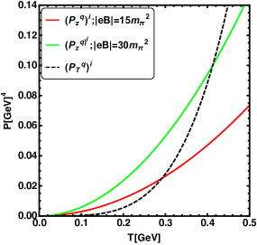
Figure 4: Variation of ideal quark pressure with and without a magnetic field as a function of temperature.

For ideal quark-gluon gas the gluons remain unaffected but quarks are strongly affected in the presence of a magnetic field. So in Fig. 4 we display a variation of the ideal quark pressure with [($P_{z}^{q})^{\text{i}}$ in Eq. (90)] and without [($P_{T}^{q})^{\text{i}}$ in Eq. (88)] magnetic field as a function of temperature. The ideal quark pressure,$(P_{z}^{q})^{\text{i}}$ , in the presence of a magnetic field is proportional to $(eB)T^{2}$ whereas that in the absence of a magnetic field, $(P_{T}^{q})^{\text{i}}$, is proportional to $T^{4}$. For a given magnetic field, $T^{2}$ dominates at low T whereas $T^{4}$ dominates at high $T$, and thus a crossing takes place at an intermediate temperature as seen in Fig. 4. Also the ideal longitudinal pressure increases linearly with the increase of the magnetic field as can be seen from Eq. (90).

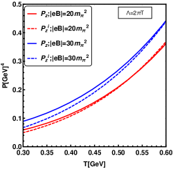
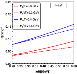
Figure 5: Variation of one-loop longitudinal pressure as a function of temperature for different values of the magnetic field (left panel) and as a function of the magnetic field at different temperatures (right panel) for $N_{f}=3$ and the central value of the renormalization scale, $\Lambda=2\pi T$. Dashed curves represent ideal longitudinal pressure.

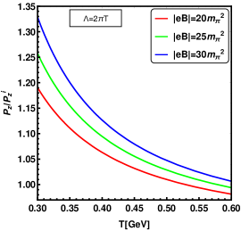
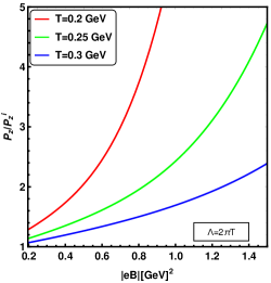
Figure 6: Variation of the one-loop longitudinal pressure scaled with the ideal longitudinal pressure as a function of temperature (left panel) for different values of the magnetic field and as a function of the magnetic field (right panel) for different temperatures with $N_{f}=3$.

The left panel of Fig. 5 displays a comparison of one-loop longitudinal pressure (solid curve) and ideal pressure (dashed curve) with temperatures for different values of field strength, whereas the right panel displays the same but with the strength of the magnetic field for different temperatures. In both cases one-loop pressure increases with the increase in temperature and field strength, respectively. However, the one-loop interacting pressure is higher than that of the ideal one in both panels. This enhancement can be understood as follows: in one-loop order both the effective quark two-point function and the effective gluon two-point function containing a quark loop are strongly affected in the presence of the magnetic field, which contribute to the additional pressure compared to the ideal case. For a given magnetic field this enhancement is stronger in the temperature domain $(300-500)$ MeV as can be seen from the scaled pressure with with ideal one ($P_{z}/P_{z}^{\text{i}}$) in the left panel of Fig. 6. However, this enhancement gradually decreases with increase of temperature and approaches to ideal value at high temperature. For a given temperature the ratio ($P_{z}/P_{z}^{\text{i}}$) increases with the increase of magnetic field strength as found in the right panel of Fig. 6. This is because $P_{z}^{\text{i}}$ has linear dependence on $eB$ whereas $P_{z}$ has a higher power dependence on $eB$.

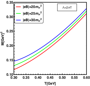
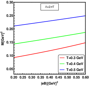
Figure 7: Variation of magnetization with temperatures for different magnetic fields (left panel) and with magnetic fields for various temperatures (right panel).

The magnetization of an ideal quark-gluon gas in the presence of a magnetic field has already been discussed in Sec. V.3. Now the magnetization of an interacting quark-gluon system is calculated using Eq. (85) and it is proportional to $[aT^{2}+b(eB)+c(eB)^{2}/T^{2}+d(eB)^{3}/T^{4}+f(eB)^{4}/T^{6}]$ which is plotted in Fig. 7. So for a given value of $eB$, at low $T$ limit $1/T^{n}$ with $n=2,4,6$ terms dominate but are restricted by the scale $gT$, whereas at high $T$, $T^{2}$ terms dominate which is seen from the left panel. In contrast to the ideal quark-gluon gas the magnetization of an interacting quark-gluon system increases with the magnetic field that is displayed in the right panel. This trend is in agreement with LQCD results Bali:2013owa . In the strong magnetic field approximation $g^{2}T^{2}<T^{2}<eB$, the magnetization acquires positive values with range $0<M<1$. So the deconfined QCD matter in the presence of a strong magnetic field within one-loop HTL approximation shows a paramagnetic nature (i.e., magnetization is parallel to the field direction) Bali:2013owa . Since the magnetization in a strong field limit increases with the magnetic field, it causes an increase in pressure of the system along the field direction, i.e., longitudinal direction. This in turn also strongly affects the transverse pressure as we would see below.

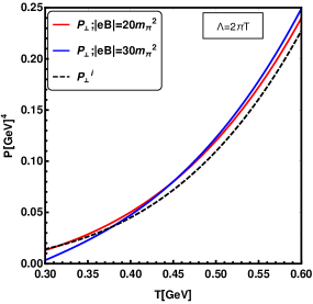
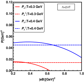
Figure 8: Variation of the one-loop transverse pressure as a function of temperature for various magnetic fields (left panel) and as a function of magnetic fields for different temperatures (right panel). Dashed curves represent the ideal transverse pressure.

One-loop transverse pressure is calculated using Eq. (86). It is evident from Eq. (86) and from the left panel of Fig. 8 that the one-loop transverse pressure increases with temperature and shows a nature similar to longitudinal pressure (left panel of Fig. 5) but lower in magnitude. Dashed lines represent the transverse ideal pressure which is independent of a magnetic field as given in Eq. (92). For a given high value of a magnetic field the pressure starts with a lower value than that of the ideal gas particularly at low $T$, and then a crossing takes place. This could also be understood from the right panel. In the right panel the transverse pressure is displayed as a function of the magnetic field for two different temperatures. Also the dashed lines here represent the ideal transverse pressure that is independent of the magnetic field. The transverse pressure for the interacting case is given in Eq. (86) as $P_{\perp}=P_{z}-eB\cdot M$. Now for a given temperature its variation is very slow (or almost remain unaltered) with a lower value of the magnetic field because there is a competition between $P_{z}$ and $eBM$. Since the magnetization $M$ increases steadily with magnetic the field (right panel of Fig. 7) the transverse pressure, $P_{\perp}$, tends to decrease, falls below the ideal gas value and may even go to negative values for low $T$ at a large value of the magnetic field. This is an indication that the system may shrink in the transverse direction Bali:2013owa .

VII Conclusion

We consider the deconfined QCD matter in the presence of the strong background magnetic field within the HTL approximation. Quarks are directly affected by the external magnetic field. In strong field approximation we assume the quarks are in the lowest Landau level. Gluons are affected through the quark loop in the gluon two-point function. Hard and soft contributions of quark-gluon free energy are calculated within the one-loop HTL approximation. Various divergent terms are eliminated by choosing appropriate counterterms in the $\overline{MS}$ renormalization scheme. In the presence of a strong magnetic field the hot QCD matter acquires paramagnetic nature. The presence of magnetization makes the system anisotropic and one gets different pressures in direction parallel and perpendicular to the magnetic field. Both longitudinal (along magnetic field direction) and transverse (perpendicular to the magnetic field direction) pressures are evaluated completely analytically by calculating the magnetization of the system. Various thermodynamic properties can be studied using the obtained free energy here. Moreover, the anisotropic pressure obtained here may be useful for a magnetohydrodynamics description and analysis of elliptic flow of hot and dense deconfined QCD matter created in heavy-ion collisions. Finally we note that since we have considered the one-loop HTL perturbation theory up to $\mathcal{O}[g^{4}]$, $\mathcal{O}[g^{2}]$ and $\mathcal{O}[g^{4}]$ are incomplete. The present result could be improved by going to higher loop orders.

VIII Acknowledgments

B.K., R.G., and M.G.M. were funded by Department of Atomic Energy (DAE), India via the project TPAES. A.B. acknowledges the support from the research grants from Conselho Nacional de Desenvolvimento Científico e Tecnológico (CNPq), under grant Coordenação de Aperfeiçoamento de Pessoal de Nível Superior (CAPES), Govt of Brazil. N.H. was funded by DAE, India. B.K. acknowledges helpful discussions with Anwesha Chattopadhyay.

Appendix A Calculation of form factors

Before computing the quark form factors, we first decompose the transverse and the longitudinal parts from the expression of the self-energy in Eq. (29). Considering the transverse parts of the fermionic momenta to be relatively weaker in the strong field limit, we make an assumption that $(K-P)_{\perp}<(K-P)_{\shortparallel}$. Then we can write down the gluonic propagator as

$$\Delta(K-P) = \frac{1}{(K-P)_{\shortparallel}^{2}-(k-p)_{\perp}^{2}}=\frac{1}{(K-P)_{\shortparallel}^{2}}\left[1-\frac{(k-p)_{\perp}^{2}}{(K-P)_{\shortparallel}^{2}}\right]^{-1}$$ (95)

$$\approx \frac{1}{(K-P)_{\shortparallel}^{2}}\left(1+\frac{(k-p)_{\perp}^{2}}{(K-P)_{\shortparallel}^{2}}\right)$$

$$= \Delta_{\shortparallel}(K-P)+(k-p)_{\perp}^{2}\Delta_{\shortparallel}^{2}(K-P).$$

A.1 Calculation of quark form factor $a$

We calculate the form factor $a$ by using Eqs. (32) and (95) as

$$a=\frac{1}{4}\operatorname{\text{Tr}}[\Sigma/\!\!\!\!u] = -2g^{2}C_{F}\sum\!\!\!\!\!\!\!\!\!\!\int\limits_{\{K\}}e^{-\frac{k_{\perp}^{2}}{q_{f}B}}\left[\frac{k_{0}}{K_{\shortparallel}^{2}(K-P)^{2}_{\shortparallel}}+(k-p)_{\perp}^{2}\frac{k_{0}}{K_{\shortparallel}^{2}(K-P)^{4}_{\shortparallel}}\right]$$ (96)

$$= -2g^{2}C_{F}\int\frac{d^{3}k}{(2\pi)^{3}}e^{-\frac{k_{\perp}^{2}}{q_{f}B}}\left[T_{2}+(k-p)_{\perp}^{2}T_{4}\right]$$

$$= -2g^{2}C_{F}\int_{-\infty}^{\infty}\frac{dk_{3}}{2\pi}\left[\frac{q_{f}B}{4\pi}T_{2}+\frac{q_{f}B}{4\pi}(p_{\perp}^{2}+q_{f}B)\hskip 5.69046ptT_{4}\right]$$

$$= -\frac{g^{2}C_{F}(q_{f}B)}{4\pi^{2}}\int_{-\infty}^{\infty}dk_{3}\left[T_{2}+(p_{\perp}^{2}+q_{f}B)\hskip 5.69046ptT_{4}\right],$$

where

$$T_{2} = \sum\frac{k_{0}}{K_{\shortparallel}^{2}(K-P)^{2}_{\shortparallel}},$$

$$T_{4} = \sum\frac{k_{0}}{K_{\shortparallel}^{2}(K-P)^{4}_{\shortparallel}}=-\frac{1}{2k_{3}}\frac{\partial T_{2}}{\partial p_{3}}.$$ (97)

Here we also note that in LLL, $p_{\perp}=0$. Now

$$T_{2} = -\frac{1}{4q_{3}}\Bigg{[}\left(1+n_{B}(q_{3})-n_{F}(k_{3})\right)\left(\frac{1}{p_{0}+k_{3}+q_{3}}+\frac{1}{p_{0}-k_{3}-q_{3}}\right)$$ (98)

$$+\big{(}n_{B}(q_{3})+n_{F}(k_{3})\big{)}\left(\frac{1}{p_{0}-k_{3}+q_{3}}+\frac{1}{p_{0}+k_{3}-q_{3}}\right)\Bigg{]}$$

$$\approx -\frac{1}{4k_{3}}\Bigg{[}\left(n_{B}(k_{3})-p_{3}\frac{\partial n_{B}(k_{3})}{\partial k_{3}}+n_{F}(k_{3})\right)\left(\frac{1}{p_{0}-p_{3}}+\frac{1}{p_{0}+p_{3}}\right)\Bigg{]}$$

$$= -\frac{1}{4k_{3}}\Bigg{[}n_{F}(k_{3})+\left(n_{B}(k_{3})-p_{3}\frac{\partial n_{B}(k_{3})}{\partial k_{3}}\right)\Bigg{]}\frac{2p_{0}}{p_{0}^{2}-p_{3}^{2}}.$$

$$\int_{-\infty}^{\infty}dk_{3}\,T_{2} = \frac{2p_{0}}{p_{0}^{2}-p_{3}^{2}}\bigg{[}-\frac{1}{4}\int\frac{dk_{3}}{k_{3}}\left(n_{F}(k_{3})+n_{B}(k_{3})-p_{3}\frac{\partial n_{B}}{\partial k_{3}}\right)\bigg{]}$$ (99)

$$\approx \frac{2p_{0}}{p_{0}^{2}-p_{3}^{2}}\bigg{[}-\frac{1}{2}\int_{0}^{\infty}dk_{3}\,\frac{n_{F}}{k_{3}}-\frac{1}{2}\int_{0}^{\infty}dk_{3}\,\frac{n_{B}}{k_{3}}\bigg{]}$$

$$= \frac{p_{0}}{p_{0}^{2}-p_{3}^{2}}\bigg{[}\left(\frac{1}{4\epsilon}+\frac{\gamma_{E}}{2}+\frac{1}{2}\ln{\frac{2}{\pi}}\right)+\left(-\frac{1}{4\epsilon}-\frac{\gamma_{E}}{2}+\frac{1}{2}\ln{2\pi}\right)\bigg{]}+\mathcal{O}[\epsilon]$$

$$= \frac{p_{0}}{p_{0}^{2}-p_{3}^{2}}\ln 2.$$

Similarly, we get

$$\int_{-\infty}^{\infty}dk_{3}\,T_{4} = -\frac{1}{2}\frac{\partial}{\partial p_{3}}\int_{-\infty}^{\infty}\frac{dk_{3}}{k_{3}}T_{4}$$ (100)

$$= -\frac{\zeta^{\prime}(-2)}{2T^{2}}\frac{p_{0}(p_{0}^{2}+p_{3}^{2})}{(p_{0}^{2}-p_{3}^{2})^{2}}.$$

So

$$a=-d=-\frac{g^{2}C_{F}(q_{f}B)}{4\pi^{2}}\bigg{[}\frac{p_{0}}{p_{0}^{2}-p_{3}^{2}}\ln 2-q_{f}B\frac{\zeta^{\prime}(-2)}{2T^{2}}\frac{p_{0}(p_{0}^{2}+p_{3}^{2})}{(p_{0}^{2}-p_{3}^{2})^{2}}\bigg{]}.$$ (101)

A.2 Calculation of quark form factor $b$

Similarly, one can calculate $b$ from Eqs. (33) and (95) as

$$b=-\frac{1}{4}\operatorname{\text{Tr}}[\Sigma/\!\!\!\!n] = 2g^{2}C_{F}\sum\!\!\!\!\!\!\!\!\!\!\int\limits_{\{K\}}e^{-\frac{k_{\perp}^{2}}{q_{f}B}}\left[\frac{k_{3}}{K_{\shortparallel}^{2}(K-P)^{2}_{\shortparallel}}+(k-p)_{\perp}^{2}\frac{k_{3}}{K_{\shortparallel}^{2}(K-P)^{4}_{\shortparallel}}\right]$$ (102)

$$= 2g^{2}C_{F}\int\frac{d^{3}k}{(2\pi)^{3}}e^{-\frac{k_{\perp}^{2}}{q_{f}B}}\,k_{3}\,\left[T_{1}+(k-p)_{\perp}^{2}T_{3}\right]$$

$$= 2g^{2}C_{F}\int_{-\infty}^{\infty}\frac{dk_{3}}{2\pi}\,k_{3}\,\left[\frac{q_{f}B}{4\pi}T_{1}+\frac{q_{f}B}{4\pi}(q_{f}B)\hskip 5.69046ptT_{3}\right]$$

$$= \frac{g^{2}C_{F}(q_{f}B)}{4\pi^{2}}\int_{-\infty}^{\infty}dk_{3}\hskip 5.69046ptk_{3}\left[T_{1}+q_{f}B\hskip 5.69046ptT_{3}\right],$$

where

$$T_{1} = \sum\frac{1}{K_{\shortparallel}^{2}(K-P)^{2}_{\shortparallel}},$$

$$T_{3} = \sum\frac{1}{K_{\shortparallel}^{2}(K-P)^{4}_{\shortparallel}}=-\frac{1}{2k_{3}}\frac{\partial T_{1}}{\partial p_{3}}.$$ (103)

Now

$$T_{1} = \frac{1}{4k_{3}q_{3}}\Bigg{[}\left(1+n_{B}(q_{3})-n_{F}(k_{3})\right)\left(\frac{1}{p_{0}+k_{3}+q_{3}}-\frac{1}{p_{0}-k_{3}-q_{3}}\right)$$ (104)

$$+\left(n_{B}(q_{3})+n_{F}(k_{3})\right)\left(\frac{1}{p_{0}+k_{3}-q_{3}}-\frac{1}{p_{0}-k_{3}+q_{3}}\right)\Bigg{]}$$

$$\approx \frac{1}{4k_{3}^{2}}\Bigg{[}\left(n_{B}(k_{3})-p_{3}\frac{\partial n_{B}(k_{3})}{\partial k_{3}}-n_{F}(k_{3})\right)\frac{1}{k_{3}}+\bigg{(}n_{B}(k_{3})-p_{3}\frac{\partial n_{B}(k_{3})}{\partial k_{3}}$$

$$+n_{F}(k_{3})\bigg{)}\left(\frac{1}{p_{0}+p_{3}}-\frac{1}{p_{0}-p_{3}}\right)\Bigg{]}$$

$$= \frac{1}{4k_{3}^{2}}\Bigg{[}\left(n_{B}(k_{3})-p_{3}\frac{\partial n_{B}(k_{3})}{\partial k_{3}}-n_{F}(k_{3})\right)\frac{1}{k_{3}}$$

$$+\left(n_{B}(k_{3})-p_{3}\frac{\partial n_{B}(k_{3})}{\partial k_{3}}+n_{F}(k_{3})\right)\left(\frac{-2p_{3}}{p_{0}^{2}-p_{3}^{2}}\right)\Bigg{]}.$$

$$\mbox{Let\,\,\,}\int_{-\infty}^{\infty}dk_{3}\hskip 5.69046ptk_{3}\,T_{1} = I_{1}\,\,{\mbox{with}}$$ (105)

$$I_{1} = \int_{-\infty}^{\infty}dk_{3}\frac{1}{4k_{3}}\Bigg{[}\left(n_{B}(k_{3})-p_{3}\frac{\partial n_{B}(k_{3})}{\partial k_{3}}-n_{F}(k_{3})\right)\frac{1}{k_{3}}$$ (106)

$$~{}~{}~{}~{}~{}~{}~{}~{}~{}~{}~{}~{}~{}~{}~{}~{}~{}~{}~{}~{}~{}~{}~{}+\left(n_{B}(k_{3})-p_{3}\frac{\partial n_{B}(k_{3})}{\partial k_{3}}+n_{F}(k_{3})\right)\left(\frac{-2p_{3}}{p_{0}^{2}-p_{3}^{2}}\right)\Bigg{]}.$$

The fermion part of $I_{1}$ can be written as

$$-\int_{-\infty}^{\infty}dk_{3}\frac{n_{F}(k_{3})}{4k_{3}}\left(\frac{1}{k_{3}}+\frac{2p_{3}}{p_{0}^{2}-p_{3}^{2}}\right) \approx -\int_{0}^{\infty}dk_{3}\,\,\frac{1}{4}\left(\frac{2n_{F}}{k_{3}}\frac{2p_{3}}{p_{0}^{2}-p_{3}^{2}}\right)$$ (107)

$$= \frac{p_{3}}{p_{0}^{2}-p_{3}^{2}}\left[\frac{1}{4\epsilon}+\frac{\gamma_{E}}{2}+\frac{1}{2}\ln{\frac{2}{\pi}}\right]+\mathcal{O}[\epsilon].$$

The bosonic part of $I_{1}$ is given as

$$\int_{-\infty}^{\infty}dk_{3}\,\frac{1}{4k_{3}}\left(n_{B}(k_{3})-p_{3}\frac{dn_{B}}{dk_{3}}\right)\left(\frac{1}{k_{3}}-\frac{2p_{3}}{p_{0}^{2}-p_{3}^{2}}\right)$$ (108)

$$\approx \frac{1}{4}\left[-2\int_{0}^{\infty}dk_{3}\,\frac{n_{B}(k_{3})}{k_{3}}\frac{2p_{3}}{p_{0}^{2}-p_{3}^{2}}-2\int_{0}^{\infty}dk_{3}\,\frac{p_{3}}{k_{3}^{2}}\frac{dn_{B}}{dk_{3}}\right]$$

$$= \frac{1}{4}\left[-2\int_{0}^{\infty}dk_{3}\,\frac{n_{B}(k_{3})}{k_{3}}\frac{2p_{3}}{p_{0}^{2}-p_{3}^{2}}-\frac{2p_{3}}{T}\frac{\partial}{\partial\beta}\int_{0}^{\infty}dk_{3}\,\frac{n_{B}(k_{3})}{k_{3}^{3}}\right]$$

$$= \frac{p_{3}}{p_{0}^{2}-p_{3}^{2}}\left(-\frac{1}{4\epsilon}-\frac{\gamma_{E}}{2}+\frac{1}{2}\ln{2\pi}\right)-\frac{p_{3}\zeta^{\prime}[-2]}{2T^{2}}+\mathcal{O}[\epsilon].$$

After combining (107) and (108), $I_{1}$ can be written as

$$I_{1} = \frac{p_{3}}{p_{0}^{2}-p_{3}^{2}}\ln{2}-\frac{p_{3}\zeta^{\prime}[-2]}{2T^{2}},$$ (109)

$$\int_{-\infty}^{\infty}dk_{3}\hskip 5.69046ptk_{3}\,T_{3} = -\frac{1}{2}\frac{\partial}{\partial p_{3}}\int dk_{3}\,T_{1}$$ (110)

$$\approx -\frac{1}{2}\frac{\partial}{\partial p_{3}}\Bigg{[}-\frac{1}{2}\int_{0}^{\infty}dk_{3}\,\frac{n_{F}(k_{3})}{k_{3}^{3}}+\frac{1}{2}\int_{0}^{\infty}dk_{3}\,\,\frac{n_{B}(k_{3})}{k_{3}^{3}}$$

$$+\frac{p_{3}}{T(p_{0}^{2}-p_{3}^{2})}\frac{\partial}{\partial\beta}\int_{0}^{\infty}dk_{3}\,\frac{n_{B}(k_{3})}{k_{3}^{3}}\Bigg{]}$$

$$= -\frac{\zeta[-2]}{T^{2}}\frac{p_{0}^{2}p_{3}}{(p_{0}^{2}-p_{3}^{2})^{2}}.$$

So,

$$b=-c=\frac{g^{2}C_{F}(q_{f}B)}{4\pi^{2}}\bigg{[}\frac{p_{3}}{p_{0}^{2}-p_{3}^{2}}\ln 2-\frac{p_{3}}{2T^{2}}\zeta^{\prime}(-2)-q_{f}B\frac{\zeta^{\prime}(-2)}{T^{2}}\frac{p_{0}^{2}p_{3}}{(p_{0}^{2}-p_{3}^{2})^{2}}\bigg{]}.$$ (111)

Appendix B One-loop sum-integrals for quark free energy

We write the form factors $a$ and $b$ as

$$a = c_{1}\bigg{[}\frac{p_{0}}{p_{0}^{2}-p_{3}^{2}}c_{2}-d_{1}\frac{p_{0}(p_{0}^{2}+p_{3}^{2})}{(p_{0}^{2}-p_{3}^{2})^{2}}\bigg{]}$$

$$= c_{1}\bigg{[}\frac{p_{0}}{P^{2}}c_{2}-d_{1}\left(\frac{p_{0}}{P^{2}}+\frac{2p_{0}p_{3}^{2}}{P^{4}}\right)\bigg{]},$$

$$b = -c_{1}\bigg{[}\frac{p_{3}}{p_{0}^{2}-p_{3}^{2}}c_{2}-p_{3}d_{2}-2d_{1}\frac{p_{0}^{2}p_{3}}{(p_{0}^{2}-p_{3}^{2})^{2}}\bigg{]}$$ (112)

$$= -c_{1}\bigg{[}\frac{p_{3}}{P^{2}}c_{2}-p_{3}d_{2}-2d_{1}\left(\frac{p_{3}}{P^{2}}+\frac{p_{3}^{3}}{P^{4}}\right)\bigg{]},$$

where

$$c_{1} = -\frac{g^{2}C_{F}(q_{f}B)}{4\pi^{2}}\,\,,\,\,c_{2}=\ln{2}\,\,,\,\,d_{1}=q_{f}B\frac{\zeta^{\prime}(-2)}{2T^{2}}\,\,,\,\,d_{2}=\frac{1}{2T^{2}}\zeta^{\prime}(-2).$$ (113)

Now one can write the following frequency sum as ‌

$$\sum\!\!\!\!\!\!\!\!\!\!\int\limits_{\{p_{0}\}}~{}\frac{ap_{0}}{P_{\shortparallel}^{2}} = c_{1}\sum\!\!\!\!\!\!\!\!\!\!\int\limits_{\{p_{0}\}}\bigg{[}\left(c_{2}-d_{1}\right)\frac{1}{P_{\shortparallel}^{2}}+\left(c_{2}-d_{1}\right)\frac{p_{3}^{2}}{P_{\shortparallel}^{4}}-2d_{1}\left(\frac{p_{3}^{2}}{P_{\shortparallel}^{4}}+\frac{p_{3}^{4}}{P_{\shortparallel}^{6}}\right)\bigg{]},$$ (114)

$$\sum\!\!\!\!\!\!\!\!\!\!\int\limits_{\{p_{0}\}}~{}\frac{bp_{3}}{P_{\shortparallel}^{2}} = -c_{1}\sum\!\!\!\!\!\!\!\!\!\!\int\limits_{\{p_{0}\}}\bigg{[}\left(c_{2}-2d_{1}\right)\frac{p_{3}^{2}}{P_{\shortparallel}^{4}}-d_{2}\frac{p_{3}^{2}}{P_{\shortparallel}^{2}}-2d_{1}\frac{p_{3}^{4}}{P_{\shortparallel}^{6}}\bigg{]},$$ (115)

$$\sum\!\!\!\!\!\!\!\!\!\!\int\limits_{\{p_{0}\}}\frac{a^{2}}{P_{\shortparallel}^{2}} = c_{1}^{2}\sum\!\!\!\!\!\!\!\!\!\!\int\limits_{\{p_{0}\}}\bigg{[}\frac{p_{0}^{2}}{P_{\shortparallel}^{6}}(\ln 2)^{2}+d_{1}^{2}\,\frac{p_{0}^{2}(p_{0}^{2}+p_{3}^{2})^{2}}{P^{10}}-2d_{1}\frac{p_{0}^{2}(p_{0}^{2}+p_{3}^{2})}{P_{\shortparallel}^{8}}\ln 2\bigg{]}$$ (116)

$$= c_{1}^{2}\sum\!\!\!\!\!\!\!\!\!\!\int\limits_{\{p_{0}\}}\bigg{[}(c_{2}-d_{1})^{2}\frac{1}{P_{\shortparallel}^{4}}+\left(c_{2}^{2}+5d_{1}^{2}-6c_{2}d_{1}\right)\frac{p_{3}^{2}}{P_{\shortparallel}^{6}}+4d_{1}\left(2d_{1}-c_{2}\right)$$

$$~{}~{}~{}~{}~{}~{}~{}~{}~{}\times\frac{p_{3}^{4}}{P_{\shortparallel}^{8}}+4d_{1}^{2}\frac{p_{3}^{6}}{P_{\shortparallel}^{10}}\bigg{]},$$

$$\sum\!\!\!\!\!\!\!\!\!\!\int\limits_{\{p_{0}\}}\frac{b^{2}}{P_{\shortparallel}^{2}} = c_{1}^{2}\sum\!\!\!\!\!\!\!\!\!\!\int\limits_{\{p_{0}\}}\bigg{[}\left(c_{2}-2d_{1}\right)^{2}\frac{p_{3}^{2}}{P_{\shortparallel}^{6}}+4d_{1}^{2}\frac{p_{3}^{6}}{P_{\shortparallel}^{10}}+4d_{1}\left(2d_{1}-c_{2}\right)\frac{p_{3}^{4}}{P_{\shortparallel}^{8}}$$ (117)

$$~{}~{}~{}~{}~{}~{}~{}+2d_{2}\left(2d_{1}-c_{2}\right)\frac{p_{3}^{2}}{P_{\shortparallel}^{4}}+4d_{1}d_{2}\frac{p_{3}^{4}}{P_{\shortparallel}^{6}}\bigg{]},$$

$$\sum\!\!\!\!\!\!\!\!\!\!\int\limits_{\{p_{0}\}}~{}\frac{a^{2}p_{3}^{2}}{P_{\shortparallel}^{4}} = c_{1}^{2}\sum\!\!\!\!\!\!\!\!\!\!\int\limits_{\{p_{0}\}}\bigg{[}(c_{2}-d_{1})^{2}\frac{p_{3}^{2}}{P_{\shortparallel}^{6}}+\left(c_{2}^{2}+5d_{1}^{2}-6c_{2}d_{1}\right)\frac{p_{3}^{4}}{P_{\shortparallel}^{8}}+4d_{1}\left(2d_{1}-c_{2}\right)$$ (118)

$$~{}~{}~{}~{}~{}~{}~{}~{}\times\frac{p_{3}^{6}}{P_{\shortparallel}^{10}}+4d_{1}^{2}\frac{p_{3}^{8}}{P_{\shortparallel}^{12}}\bigg{]},$$

$$\sum\!\!\!\!\!\!\!\!\!\!\int\limits_{\{p_{0}\}}~{}\frac{b^{2}p_{3}^{2}}{P_{\shortparallel}^{4}} = c_{1}^{2}\sum\!\!\!\!\!\!\!\!\!\!\int\limits_{\{p_{0}\}}\bigg{[}\left(c_{2}-2d_{1}\right)^{2}\frac{p_{3}^{4}}{P_{\shortparallel}^{8}}+4d_{1}^{2}\frac{p_{3}^{8}}{P_{\shortparallel}^{12}}+4d_{1}\left(2d_{1}-c_{2}\right)\frac{p_{3}^{6}}{P_{\shortparallel}^{10}}$$ (119)

$$~{}~{}~{}~{}~{}~{}~{}+2d_{2}\left(2d_{1}-c_{2}\right)\frac{p_{3}^{4}}{P_{\shortparallel}^{6}}+4d_{1}d_{2}\frac{p_{3}^{6}}{P_{\shortparallel}^{8}}\bigg{]},$$

$$\sum\!\!\!\!\!\!\!\!\!\!\int\limits_{\{p_{0}\}}~{}\frac{abp_{0}p_{3}}{P_{\shortparallel}^{4}} = c_{1}^{2}\sum\!\!\!\!\!\!\!\!\!\!\int\limits_{\{p_{0}\}}\bigg{[}\left(c_{2}-d_{1}\right)\left(c_{2}-2d_{1}\right)\frac{p_{3}^{2}}{P_{\shortparallel}^{6}}-d_{2}\left(c_{2}-d_{1}\right)\frac{p_{3}^{2}}{P_{\shortparallel}^{4}}$$ (120)

$$~{}~{}~{}~{}~{}~{}~{}~{}+\{\left(c_{2}-d_{1}\right)\left(c_{2}-6d_{1}\right)+2d_{1}^{2}\}\frac{p_{3}^{4}}{P_{\shortparallel}^{8}}+d_{2}\left(3d_{1}-c_{2}\right)\frac{p_{3}^{4}}{P_{\shortparallel}^{6}}$$

$$~{}~{}~{}~{}~{}~{}~{}~{}~{}+2d_{1}\left(5d_{1}-2c_{2}\right)\frac{p_{3}^{6}}{P_{\shortparallel}^{10}}+2d_{1}d_{2}\frac{p_{3}^{6}}{P_{\shortparallel}^{8}}+4d_{1}^{2}\frac{p_{3}^{8}}{P_{\shortparallel}^{12}}\bigg{]}.$$

So $F^{\prime}_{q}$ in Eq. (54) becomes

$$F^{\prime}_{q} = -4d_{F}\sum_{f}\frac{q_{f}B}{(2\pi)^{2}}\sum\!\!\!\!\!\!\!\!\!\!\int\limits_{\{p_{0}\}}dp_{3}~{}\bigg{[}\frac{ap_{0}}{P_{\shortparallel}^{2}}+\frac{bp_{3}}{P_{\shortparallel}^{2}}-\frac{a^{2}}{P_{\shortparallel}^{2}}-\frac{b^{2}}{P_{\shortparallel}^{2}}-\frac{2a^{2}p_{3}^{2}}{P_{\shortparallel}^{4}}-\frac{2b^{2}p_{3}^{2}}{P_{\shortparallel}^{4}}$$ (122)

$$~{}~{}~{}~{}~{}~{}~{}~{}~{}~{}~{}~{}~{}~{}~{}~{}~{}~{}~{}~{}~{}~{}~{}~{}~{}~{}~{}~{}~{}~{}~{}~{}~{}-\frac{4abp_{0}p_{3}}{P_{\shortparallel}^{4}}\bigg{]}$$

$$= -4d_{F}\sum_{f}\frac{q_{f}B}{(2\pi)^{2}}\bigg{[}c_{1}(c_{2}-d_{1})~{}\sum\!\!\!\!\!\!\!\!\!\!\int\limits_{\{p_{0}\}}~{}\frac{1}{P_{\shortparallel}^{2}}-c_{1}\big{(}d_{1}-6c_{1}c_{2}d_{2}$$

$$+8c_{1}d_{1}d_{2}\big{)}\sum\!\!\!\!\!\!\!\!\!\!\int\limits_{\{p_{0}\}}~{}\frac{p_{3}^{2}}{P_{\shortparallel}^{4}}+8c_{1}^{2}d_{2}\left(c_{2}-3d_{1}\right)\sum\!\!\!\!\!\!\!\!\!\!\int\limits_{\{p_{0}\}}~{}\frac{p_{3}^{4}}{P_{\shortparallel}^{6}}-16c_{1}^{2}d_{1}d_{2}\sum\!\!\!\!\!\!\!\!\!\!\int\limits_{\{p_{0}\}}~{}\frac{p_{3}^{6}}{P_{\shortparallel}^{8}}$$

$$+c_{1}d_{2}\sum\!\!\!\!\!\!\!\!\!\!\int\limits_{\{p_{0}\}}~{}\frac{p_{3}^{2}}{P_{\shortparallel}^{2}}-c_{1}^{2}\left(c_{2}-d_{1}\right)^{2}\sum\!\!\!\!\!\!\!\!\!\!\int\limits_{\{p_{0}\}}~{}\frac{1}{P_{\shortparallel}^{4}}-c_{1}^{2}\left(8c_{2}^{2}-26c_{2}d_{1}+19d_{1}^{2}\right)$$

$$\sum\!\!\!\!\!\!\!\!\!\!\int\limits_{\{p_{0}\}}~{}\frac{p_{3}^{2}}{P_{\shortparallel}^{6}}-2c_{1}^{2}\left(2c_{2}-11d_{1}\right)\left(2c_{2}-3d_{1}\right)\sum\!\!\!\!\!\!\!\!\!\!\int\limits_{\{p_{0}\}}~{}\frac{p_{3}^{4}}{P_{\shortparallel}^{8}}-16c_{1}^{2}d_{1}\left(-2c_{2}+5d_{1}\right)$$

$$\times\sum\!\!\!\!\!\!\!\!\!\!\int\limits_{\{p_{0}\}}~{}\frac{p_{3}^{6}}{P_{\shortparallel}^{10}}-32c_{1}^{2}d_{1}^{2}\sum\!\!\!\!\!\!\!\!\!\!\int\limits_{\{p_{0}\}}~{}\frac{p_{3}^{8}}{P_{\shortparallel}^{12}}\bigg{]}.$$

Now we calculate the frequency sums as

$$\sum_{\{p_{0}\}}\frac{1}{P_{\shortparallel}^{4}} = \frac{1}{2p_{3}}\frac{\partial}{\partial p_{3}}\sum_{\{p_{0}\}}\frac{1}{P_{\shortparallel}^{2}},$$

$$\sum_{\{p_{0}\}}\frac{1}{P_{\shortparallel}^{6}} = \frac{1}{4p_{3}}\frac{\partial}{\partial p_{3}}\sum_{\{p_{0}\}}\frac{1}{P_{\shortparallel}^{4}},$$

$$\sum_{\{p_{0}\}}\frac{1}{P_{\shortparallel}^{8}} = \frac{1}{6p_{3}}\frac{\partial}{\partial p_{3}}\sum_{\{p_{0}\}}\frac{1}{P_{\shortparallel}^{6}},$$

$$\sum_{\{p_{0}\}}\frac{1}{P_{\shortparallel}^{10}} = \frac{1}{8p_{3}}\frac{\partial}{\partial p_{3}}\sum_{\{p_{0}\}}\frac{1}{P_{\shortparallel}^{8}}.$$ (123)

One can calculate

$$\sum_{\{p_{0}\}}\frac{1}{P_{\shortparallel}^{2}} = -\frac{1}{2p_{3}}\bigg{(}1-2\,n_{F}(p_{3})\bigg{)},$$ (124)

Thus using Eq. (124) in Eq. (B), one can write

$$\sum_{\{p_{0}\}}\frac{1}{P_{\shortparallel}^{4}}\! = \!\frac{1}{2p_{3}}\frac{\partial}{\partial p_{3}}\bigg{(}\sum_{\{p_{0}\}}\frac{1}{P_{\shortparallel}^{2}}\bigg{)}\!\approx\!\frac{1}{2p_{3}}\frac{\partial}{\partial p_{3}}\bigg{[}\frac{n_{F}(p_{3})}{p_{3}}\bigg{]}\!\!=\!\!\frac{1}{2p_{3}}\bigg{[}\frac{\beta}{p_{3}^{2}}\frac{\partial n_{F}(p_{3})}{\partial\beta}-\frac{n_{F}(p_{3})}{p_{3}^{2}}\bigg{]}.$$ (125)

Now we perform the sum-integrals in Eq. (122) as

$$\sum\!\!\!\!\!\!\!\!\!\!\int\limits_{\{p_{0}\}}\,\frac{1}{P_{\shortparallel}^{4}} = \left(\frac{e^{\gamma_{E}}\Lambda^{2}}{4\pi}\right)^{\epsilon}\int_{-\infty}^{\infty}d^{1-2\epsilon}p_{3}\left(\beta\frac{\partial}{\partial\beta}-1\right)\frac{n_{F}(p_{3})}{2p_{3}^{3}}$$ (126)

$$\approx 2\left(\frac{e^{\gamma_{E}}\Lambda^{2}}{4\pi}\right)^{\epsilon}\int_{0}^{\infty}d^{1-2\epsilon}p_{3}\left(\beta\frac{\partial}{\partial\beta}-1\right)\frac{n_{F}(p_{3})}{2p_{3}^{3}}$$

$$\approx \left(\frac{\Lambda}{4\pi T}\right)^{2\epsilon}\left[-\frac{7}{2}\frac{\zeta^{{}^{\prime}}(-2)}{T^{2}}+O(\epsilon)\right],$$

$$\sum\!\!\!\!\!\!\!\!\!\!\int\limits_{\{p_{0}\}}\,\frac{p_{3}^{2}}{P_{\shortparallel}^{6}} = \left(\frac{e^{\gamma_{E}}\Lambda^{2}}{4\pi}\right)^{\epsilon}{\int_{-\infty}^{\infty}d^{1-2\epsilon}p_{3}\left(\beta^{2}\frac{\partial^{2}}{\partial\beta^{2}}-3\beta\frac{\partial}{\partial\beta}+3\right)\frac{n_{F}(p_{3})}{8p_{3}^{3}}}$$ (127)

$$\approx \left(\frac{\Lambda}{4\pi T}\right)^{2\epsilon}\left[{\frac{7}{8}\frac{\zeta^{{}^{\prime}}(-2)}{T^{2}}+O(\epsilon)}\right],$$

$$\sum\!\!\!\!\!\!\!\!\!\!\int\limits_{\{p_{0}\}}\,\frac{p_{3}^{4}}{P_{\shortparallel}^{8}} = \left(\frac{e^{\gamma_{E}}\Lambda^{2}}{4\pi}\right)^{\epsilon}\int_{-\infty}^{\infty}d^{1-2\epsilon}p_{3}\left(\beta^{3}\frac{\partial^{3}}{\partial\beta^{3}}-6\beta^{2}\frac{\partial^{2}}{\partial\beta^{2}}+15\beta\frac{\partial}{\partial\beta}-15\right)\frac{n_{F}(p_{3})}{48p_{3}^{3}}$$ (128)

$$\approx \left(\frac{\Lambda}{4\pi T}\right)^{2\epsilon}\left[-\frac{7}{16}\frac{\zeta^{{}^{\prime}}(-2)}{T^{2}}+O(\epsilon)\right],$$

$$\sum\!\!\!\!\!\!\!\!\!\!\int\limits_{\{p_{0}\}}\,\frac{p_{3}^{6}}{P_{\shortparallel}^{10}} = \left(\frac{e^{\gamma_{E}}\Lambda^{2}}{4\pi}\right)^{\epsilon}\int_{-\infty}^{\infty}d^{1-2\epsilon}p_{3}\bigg{(}\beta^{4}\frac{\partial^{4}}{\partial\beta^{4}}-10\beta^{3}\frac{\partial^{3}}{\partial\beta^{3}}+45\beta^{2}\frac{\partial^{2}}{\partial\beta^{2}}-105\beta\frac{\partial}{\partial\beta}$$ (129)

$$+105\bigg{)}\frac{n_{F}(p_{3})}{384p_{3}^{3}}$$

$$\approx \left(\frac{\Lambda}{4\pi T}\right)^{2\epsilon}\left[\frac{35}{256}\frac{\zeta^{{}^{\prime}}(-2)}{T^{2}}+O(\epsilon)\right],$$

$$\sum\!\!\!\!\!\!\!\!\!\!\int\limits_{\{p_{0}\}}\,\frac{p_{3}^{8}}{P_{\shortparallel}^{12}} = \left(\frac{e^{\gamma_{E}}\Lambda^{2}}{4\pi}\right)^{\epsilon}\int_{-\infty}^{\infty}d^{1-2\epsilon}p_{3}\bigg{(}\beta^{5}\frac{\partial^{5}}{\partial\beta^{5}}-15\beta^{4}\frac{\partial^{4}}{\partial\beta^{4}}+105\beta^{3}\frac{\partial^{3}}{\partial\beta^{3}}$$ (130)

$$-420\beta^{2}\frac{\partial^{2}}{\partial\beta^{2}}+945\beta\frac{\partial}{\partial\beta}-945\bigg{)}\frac{n_{F}(p_{3})}{3840p_{3}^{3}}$$

$$\approx \left(\frac{\Lambda}{4\pi T}\right)^{2\epsilon}\left[-\frac{49}{256}\frac{\zeta^{\prime}(-2)}{T^{2}}+O(\epsilon)\right].$$

Similarly one can calculate

$$\sum\!\!\!\!\!\!\!\!\!\!\int\limits_{\{p_{0}\}}\,\frac{1}{P_{\shortparallel}^{2}} = \left(\frac{e^{\gamma_{E}}\Lambda^{2}}{4\pi}\right)^{\epsilon}\int_{-\infty}^{\infty}d^{1-2\epsilon}p_{3}\,\frac{n_{F}(p_{3})}{p_{3}}$$ (132)

$$\approx \left(\frac{\Lambda}{4\pi T}\right)^{2\epsilon}\left[-\frac{1}{2\epsilon}-\frac{1}{2}\left(3\gamma_{E}+4\ln{2}-\ln{\pi}\right)+O(\epsilon)\right],$$

$$\sum\!\!\!\!\!\!\!\!\!\!\int\limits_{\{p_{0}\}}\,\frac{p_{3}^{2}}{P_{\shortparallel}^{4}} = \left(\frac{e^{\gamma_{E}}\Lambda^{2}}{4\pi}\right)^{\epsilon}\int_{-\infty}^{\infty}d^{1-2\epsilon}p_{3}\,\left(\beta\frac{\partial}{\partial\beta}-1\right)\frac{n_{F}(p_{3})}{2p_{3}}$$ (133)

$$\approx \left(\frac{\Lambda}{4\pi T}\right)^{2\epsilon}\left[\frac{1}{4\epsilon}+\frac{1}{4}\left(-2+3\gamma_{E}+4\ln{2}-\ln{\pi}\right)+O(\epsilon)\right],$$

$$\sum\!\!\!\!\!\!\!\!\!\!\int\limits_{\{p_{0}\}}\,\frac{p_{3}^{4}}{P_{\shortparallel}^{6}} = \left(\frac{e^{\gamma_{E}}\Lambda^{2}}{4\pi}\right)^{\epsilon}\int_{-\infty}^{\infty}d^{1-2\epsilon}p_{3}\,\left(\beta^{2}\frac{\partial^{2}}{\partial\beta^{2}}-3\beta\frac{\partial}{\partial\beta}+3\right)\frac{n_{F}(p_{3})}{8p_{3}}$$ (134)

$$\approx \left(\frac{\Lambda}{4\pi T}\right)^{2\epsilon}\left[-\frac{3}{16\epsilon}-\frac{3}{16}\left(-\frac{8}{3}+3\gamma_{E}+4\ln{2}-\ln{\pi}\right)+O(\epsilon)\right],$$

$$\sum\!\!\!\!\!\!\!\!\!\!\int\limits_{\{p_{0}\}}\,\frac{p_{3}^{6}}{P_{\shortparallel}^{8}} = \left(\frac{e^{\gamma_{E}}\Lambda^{2}}{4\pi}\right)^{\epsilon}\int_{-\infty}^{\infty}d^{1-2\epsilon}p_{3}\,\left(\beta^{3}\frac{\partial^{3}}{\partial\beta^{3}}-6\beta^{2}\frac{\partial^{2}}{\partial\beta^{2}}+15\beta\frac{\partial}{\partial\beta}-15\right)\frac{n_{F}}{48p_{3}}$$ (135)

$$\approx \left(\frac{\Lambda}{4\pi T}\right)^{2\epsilon}\left[\frac{5}{32\epsilon}+\frac{5}{32}\left(-\frac{46}{15}+3\gamma_{E}+4\ln{2}-\ln{\pi}\right)+O(\epsilon)\right],$$

$$\sum\!\!\!\!\!\!\!\!\!\!\int\limits_{\{p_{0}\}}\,\frac{p_{3}^{2}}{P_{\shortparallel}^{2}} = \left(\frac{\Lambda}{4\pi T}\right)^{2\epsilon}\left[\frac{\pi^{2}T^{2}}{6}+O(\epsilon)\right].$$ (136)

Using the above sum-integrals in Eq. (122) $F^{\prime}_{q}$ up to $\mathcal{O}(g^{4})$ can be written as,

$$F^{\prime}_{q} = -4d_{F}\sum_{f}\frac{\left(q_{f}B\right)^{2}}{(2\pi)^{2}}\frac{g^{2}C_{F}}{4\pi^{2}}\left(\frac{\Lambda}{4\pi T}\right)^{2\epsilon}\Bigg{[}\frac{1}{8\epsilon}\left(4\ln{2}-q_{f}B\frac{\zeta^{{}^{\prime}}(-2)}{T^{2}}\right)+\frac{1}{24576}$$ (137)

$$\times\bigg{\{}12288\ln{2}(3\gamma_{E}+4\ln{2}-\ln{\pi})+\frac{256\zeta[3]}{\pi^{4}T^{2}}\Big{(}2\pi^{4}T^{2}-3g^{2}C_{F}(q_{f}B)\ln{2}$$

$$+3\pi^{2}(q_{f}B)(2+3\gamma_{E}+4\ln{2}-\ln{\pi})\Big{)}-\frac{8g^{2}C_{F}}{\pi^{6}T^{4}}(q_{F}B)^{2}\zeta[3]^{2}(4+105\ln{2})$$

$$+\frac{7245g^{2}C_{F}}{\pi^{8}T^{6}}(q_{F}B)^{3}\zeta[3]^{3}\bigg{\}}\Bigg{]}.$$

Appendix C HTL One-loop sum-integrals for gluon free energy

$$\sum\!\!\!\!\!\!\!\!\!\int\limits_{P}\frac{1}{P^{2}} = -\frac{T^{2}}{12}\left(\frac{\Lambda}{4\pi T}\right)^{2\epsilon}\Bigg{[}1+2\epsilon\left(1+\frac{\zeta^{\prime}(-1)}{\zeta(-1)}\right)\Bigg{]}+\mathcal{O}[\epsilon]^{2},$$ (138)

$$\sum\!\!\!\!\!\!\!\!\!\int\limits_{P}\frac{1}{p^{2}P^{2}} = -\frac{2}{(4\pi)^{2}}\left(\frac{\Lambda}{4\pi T}\right)^{2\epsilon}\Bigg{[}\frac{1}{\epsilon}+2\gamma_{E}+2+\epsilon\left(4+4\gamma_{E}+\frac{\pi^{2}}{4}-4\gamma_{1}\right)\Bigg{]}$$ (139)

$$+\mathcal{O}[\epsilon]^{2},$$

$$\sum\!\!\!\!\!\!\!\!\!\int\limits_{P}\frac{1}{P^{4}} = \frac{1}{(4\pi)^{2}}\left(\frac{\Lambda}{4\pi T}\right)^{2\epsilon}\left[\frac{1}{\epsilon}+2\gamma_{E}+\epsilon\left(\frac{\pi^{2}}{4}-4\gamma_{1}\right)\right]+\mathcal{O}[\epsilon]^{2},$$ (140)

$$\sum\!\!\!\!\!\!\!\!\!\int\limits_{P}\frac{\mathcal{T}_{p}}{p^{2}P^{2}} = \sum\!\!\!\!\!\!\!\!\!\int\limits_{P}\left\langle\frac{1-c^{2\epsilon+1}}{1-c^{2}}\right\rangle_{c}\frac{1}{p^{2}P^{2}}$$ (141)

$$= -\frac{2}{(4\pi)^{2}}\left(\frac{\Lambda}{4\pi T}\right)^{2\epsilon}\left(\ln 2+\left(\frac{\pi^{2}}{6}-(2-\ln 2)\ln 2\right)\epsilon\right)\Bigg{[}\frac{1}{\epsilon}+2\gamma_{E}+2$$

$$+\epsilon\bigg{(}4+4\gamma_{E}+\frac{\pi^{2}}{4}-4\gamma_{1}\bigg{)}\Bigg{]}$$

$$= -\frac{2}{(4\pi)^{2}}\left(\frac{\Lambda}{4\pi T}\right)^{2\epsilon}\Bigg{[}\frac{1}{\epsilon}\ln 2+\frac{\pi^{2}}{6}+\left(\ln 2\right)^{2}+2\gamma_{E}\ln 2\Bigg{]},$$

$$\sum\!\!\!\!\!\!\!\!\!\int\limits_{P}\frac{\mathcal{T}_{p}}{p^{4}} = \sum\!\!\!\!\!\!\!\!\!\int\limits_{P}\left\langle c^{2\epsilon+1}\right\rangle_{c}\frac{1}{p^{2}P^{2}}$$ (142)

$$= -\frac{2}{(4\pi)^{2}}\left(\frac{\Lambda}{4\pi T}\right)^{2\epsilon}\left\{\frac{1}{2}+\left(-1+\ln 2\right)\epsilon\right\}\Bigg{[}\frac{1}{\epsilon}+2\gamma_{E}+2$$

$$+\epsilon\bigg{(}4+4\gamma_{E}+\frac{\pi^{2}}{4}-4\gamma_{1}\bigg{)}\Bigg{]}$$

$$= -\frac{2}{(4\pi)^{2}}\left(\frac{\Lambda}{4\pi T}\right)^{2\epsilon}\Bigg{[}\frac{1}{2\epsilon}+\left(\gamma_{E}+\ln 2\right)\Bigg{]},$$

$$\sum\!\!\!\!\!\!\!\!\!\int\limits_{P}\frac{\mathcal{T}_{p}^{2}}{p^{4}} = \sum\!\!\!\!\!\!\!\!\!\int\limits_{P}\left\langle\frac{c_{1}^{2\epsilon+3}-c_{2}^{2\epsilon+3}}{c_{1}^{2}-c_{2}^{2}}\right\rangle_{c}\frac{1}{p^{2}P^{2}}$$ (143)

$$= -\frac{2}{(4\pi)^{2}}\left(\frac{\Lambda}{4\pi T}\right)^{2\epsilon}\left(\frac{1}{3}(1+2\ln 2)+\frac{2}{9}\left(-5+\ln 2\left(5+3\ln 2\right)\right)\epsilon\right)$$

$$\times\Bigg{[}\frac{1}{\epsilon}+2\gamma_{E}+2+\epsilon\left(4+4\gamma_{E}+\frac{\pi^{2}}{4}-4\gamma_{1}\right)\Bigg{]}$$

$$= -\frac{2}{(4\pi)^{2}}\left(\frac{\Lambda}{4\pi T}\right)^{2\epsilon}\Bigg{[}\frac{1}{3\epsilon}\left(1+2\ln 2\right)+\frac{2}{9}\bigg{(}-2+3\left(\ln 2\right)^{2}$$

$$+\gamma_{E}(3+6\ln 2)+11\ln 2\bigg{)}\Bigg{]}.$$

$$\sum\!\!\!\!\!\!\!\!\!\int\limits_{P}e^{{-p_{\perp}^{2}}/{2q_{f}B}}\frac{1}{p^{2}P^{2}}\frac{p_{3}^{2}}{\left(p_{0}^{2}-p_{3}^{2}\right)}$$ (144)

$$= \sum\!\!\!\!\!\!\!\!\!\int\limits_{P}e^{{-p_{\perp}^{2}}/{2q_{f}B}}\frac{p_{3}^{2}}{p^{2}\left(p^{2}-p_{3}^{2}\right)}\left\{\frac{1}{P^{2}}-\frac{1}{p_{0}^{2}-p_{3}^{2}}\right\}$$

$$= \sum\!\!\!\!\!\!\!\!\!\int\limits_{P}e^{{-p_{\perp}^{2}}/{2q_{f}B}}\frac{p_{3}^{2}}{p^{2}\left(p^{2}-p_{3}^{2}\right)P^{2}}-\sum\!\!\!\!\!\!\!\!\!\int\limits_{P}e^{{-p_{\perp}^{2}}/{2q_{f}B}}\frac{p_{3}^{2}}{p^{2}\left(p^{2}-p_{3}^{2}\right)\left(p_{0}^{2}-p_{3}^{2}\right)}$$

$$= \left(\frac{e^{\gamma_{E}}\Lambda^{2}}{4\pi}\right)^{\epsilon}\int\frac{d^{3-2\epsilon}p}{(2\pi)^{3-2\epsilon}}\Bigg{[}-e^{{-p_{\perp}^{2}}/{2q_{f}B}}\frac{p_{3}^{2}}{p^{3}\left(p^{2}-p_{3}^{2}\right)}n_{B}(p)+e^{{-p_{\perp}^{2}}/{2q_{f}B}}$$

$$~{}~{}~{}~{}~{}~{}~{}~{}~{}~{}~{}~{}~{}~{}~{}\times\frac{p_{3}}{p^{2}\left(p^{2}-p_{3}^{2}\right)}n_{B}(p_{3})\Bigg{]}$$

$$\approx \left(\frac{\Lambda}{4\pi T}\right)^{2\epsilon}\frac{1}{(4\pi)^{2}9q_{f}B}\bigg{[}\frac{1}{\epsilon}\bigg{(}18q_{f}B-3\pi^{2}T^{2}-18q_{f}B\ln 2\bigg{)}+\bigg{\{}-3qfB$$

$$\bigg{(}-12+\pi^{2}+6(\ln 2)^{2}+6\gamma_{E}(-2+2\ln 2)\bigg{)}-\pi^{2}T^{2}\bigg{(}-8+6\ln 2$$

$$+6\left(1+\frac{\zeta^{\prime}[-1]}{\zeta[-1]}\right)\bigg{)}\bigg{\}}\bigg{]}+O\bigg{[}\frac{1}{(q_{f}B)^{2}}\bigg{]}.$$

$$\sum\!\!\!\!\!\!\!\!\!\int\limits_{P}e^{{-p_{\perp}^{2}}/{2q_{f_{1}}B}}e^{{-p_{\perp}^{2}}/{2q_{f_{2}}B}}\frac{p_{3}^{4}}{p^{4}\left(p_{0}^{2}-p_{3}^{2}\right)^{2}}$$ (145)

$$= -\left(\frac{e^{\gamma_{E}}\Lambda^{2}}{4\pi}\right)^{\epsilon}\int\frac{d^{3-2\epsilon}p}{(2\pi)^{3-2\epsilon}}e^{{-p_{\perp}^{2}}/{2q_{f_{1}}B}}e^{{-p_{\perp}^{2}}/{2q_{f_{2}}B}}\frac{p_{3}}{2p^{4}}\left(\beta\frac{\partial}{\partial\beta}-1\right)n_{B}(p_{3})$$

$$\approx -\left(\frac{\Lambda}{4\pi T}\right)^{2\epsilon}\frac{1}{(4\pi)^{2}}\bigg{[}\frac{T^{4}}{36(q_{f_{1}}B)^{2}(q_{f_{2}}B)^{2}\epsilon}\bigg{\{}-\frac{18{(q_{f_{1}}B)}^{2}{(q_{f_{2}}B)}^{2}}{T^{4}}+\frac{18\pi^{2}{(q_{f_{1}}B)}{q_{f_{2}}B}}{T^{2}}$$

$$\left({q_{f_{1}}B}+{q_{f_{2}}B}\right)+6\pi^{4}\left({(q_{f_{1}}B)}^{2}+{(q_{f_{2}}B)}^{2}\right)+12\pi^{4}{q_{f_{1}}B}{q_{f_{2}}B}\bigg{\}}+\frac{1}{36(q_{f_{1}}B)^{2}(q_{f_{2}}B)^{2}}$$

$$\bigg{\{}-18\bigg{(}{(q_{f_{1}}B)}^{2}\left({(q_{f_{2}}B)}^{2}\ln 4+12{q_{f_{2}}B}T^{2}\zeta^{\prime}[2]+60T^{4}\zeta^{\prime}[4]\right)+12{q_{f_{1}}B}{q_{f_{2}}B}T^{2}$$

$$\left({q_{f_{2}}B}\zeta^{\prime}[2]+10T^{2}\zeta^{\prime}[4]\right)+60{(q_{f_{2}}B)}^{2}T^{4}\zeta^{\prime}[4]\bigg{)}+12\gamma_{E}\big{(}{(q_{f_{1}}B)}^{2}\Big{(}-3{(q_{f_{2}}B)}^{2}$$

$$+3\pi^{2}{q_{f_{2}}B}T^{2}+\pi^{4}T^{4}\Big{)}+\pi^{2}{q_{f_{1}}B}{q_{f_{2}}B}T^{2}\left(3{q_{f_{2}}B}+2\pi^{2}T^{2}\right)+\pi^{4}{(q_{f_{2}}B)}^{2}T^{4}\big{)}$$

$$+\pi^{4}T^{4}(12\ln(4\pi)-25)({q_{f_{1}}B}+{q_{f_{2}}B})^{2}+18\pi^{2}{q_{f_{1}}B}{q_{f_{2}}B}T^{2}(-3+2\ln(4\pi))$$

$$({q_{f_{1}}B}+{q_{f_{2}}B})\bigg{\}}\bigg{]}+O\bigg{[}\frac{1}{(q_{f}B)^{3}}\bigg{]}.$$

$$\sum\!\!\!\!\!\!\!\!\!\int\limits_{P}e^{{-p_{\perp}^{2}}/{2q_{f}B}}\frac{p_{3}^{2}}{p^{4}\left(p_{0}^{2}-p_{3}^{2}\right)}=-\left(\frac{e^{\gamma_{E}}\Lambda^{2}}{4\pi}\right)^{\epsilon}\int\frac{d^{3-2\epsilon}p}{(2\pi)^{3-2\epsilon}}e^{{-p_{\perp}^{2}}/{2q_{f}B}}\frac{p_{3}}{p^{4}}n_{B}(p_{3})$$ (146)

$$\approx -\left(\frac{\Lambda}{4\pi T}\right)^{2\epsilon}\frac{1}{(4\pi)^{2}}\bigg{[}\frac{1}{\epsilon}\left(1-\frac{\pi^{2}T^{2}}{3q_{f}B}\right)+\frac{1}{3}\bigg{\{}-\frac{\pi^{2}T^{2}}{q_{f}B}\left(2\left(1+\frac{\zeta^{\prime}[-1]}{\zeta[-1]}\right)-3+2\ln 2\right)$$

$$+6\gamma_{E}+6\ln 2\bigg{\}}\bigg{]}+O\bigg{[}\frac{1}{(q_{f}B)^{2}}\bigg{]}.$$

$$\sum\!\!\!\!\!\!\!\!\!\int\limits_{P}e^{{-p_{\perp}^{2}}/{2q_{f}B}}\frac{p_{3}^{2}\mathcal{T}_{p}}{p^{4}\left(p_{0}^{2}-p_{3}^{2}\right)}$$ (147)

$$= \left(\frac{e^{\gamma_{E}}\Lambda^{2}}{4\pi}\right)^{\epsilon}\int\frac{d^{3-2\epsilon}p}{(2\pi)^{3-2\epsilon}}e^{{-p_{\perp}^{2}}/{2q_{f}B}}\Bigg{\langle}-\frac{p_{3}n_{B}(p_{3})}{p^{4}}-\frac{p_{3}c^{2}n_{B}(p_{3})}{p^{2}\left(p_{3}^{2}-p^{2}c^{2}\right)}+\frac{p_{3}^{2}cn_{B}(pc)}{p^{3}\left(p_{3}^{2}-p^{2}c^{2}\right)}\Bigg{\rangle}_{c}$$

$$\approx \left(\frac{\Lambda}{4\pi T}\right)^{2\epsilon}\frac{1}{(4\pi)^{2}}\bigg{[}\frac{1}{\epsilon}\bigg{(}\frac{1}{3}-\frac{2\pi^{2}T^{2}}{9q_{f}B}\bigg{)}+\frac{1}{27q_{f}B}\bigg{\{}\pi^{2}T^{2}\bigg{(}-12\left(1+\frac{\zeta^{\prime}[-1]}{\zeta[-1]}\right)$$

$$+17+12\ln 2\bigg{)}-3q_{f}B\left(-8+12(\ln 2)^{2}+18\ln 2+6\gamma_{E}(4\ln 2-1)+8\ln 2\right)\bigg{\}}\bigg{]}$$

$$+O\bigg{[}\frac{1}{(q_{f}B)^{2}}\bigg{]}.$$

Using Eqs. (138)-(147) in Eq. (71) one can get an expression for gluon free energy in a strongly magnetized medium computed up to $\mathcal{O}[g^{4}]$ as

$$F_{g} = d_{A}\frac{1}{(4\pi)^{2}}\Bigg{[}\frac{1}{\epsilon}\Bigg{\{}-\frac{1}{8}\left(\frac{C_{A}g^{2}T^{2}}{3}\right)^{2}+\sum_{f_{1},f_{2}}\frac{g^{4}T^{4}}{192(q_{f_{1}}B)(q_{f_{2}}B)}\bigg{(}{(q_{f_{1}}B)}^{2}+{(q_{f_{2}}B)}^{2}\bigg{)}$$ (148)

$$+\frac{N_{f}^{2}g^{4}T^{4}}{96}+\frac{C_{A}N_{f}g^{4}T^{4}}{36}-\sum_{f_{1},f_{2}}\frac{g^{4}(q_{f_{1}}B)(q_{f_{2}}B)}{64\pi^{4}}+\sum_{f_{1},f_{2}}\frac{g^{4}T^{2}}{64\pi^{2}}\Big{(}{q_{f_{1}}B}+{q_{f_{2}}B}\Big{)}$$

$$-\sum_{f}\frac{1}{4\pi^{2}}\frac{C_{A}g^{4}T^{2}q_{f}B}{6}\left(1+\ln 2\right)\Bigg{\}}-\frac{16\pi^{4}T^{4}}{45}+\frac{2C_{A}g^{2}\pi^{2}T^{4}}{9}+\left(\frac{C_{A}g^{2}T^{2}}{3}\right)^{2}$$

$$\times\frac{1}{12}\Big{(}8-3\gamma_{E}-\pi^{2}+7\ln 2-3\ln\hat{\Lambda}\Big{)}+\frac{1}{2}\sum_{f_{1},f_{2}}\left(\frac{g^{2}}{4\pi^{2}}\right)^{2}\Bigg{\{}\frac{1}{2}\pi^{2}T^{2}\bigg{(}2\left(1+\frac{\zeta^{\prime}[-1]}{\zeta[-1]}\right)$$

$$-3+2\ln 2\bigg{)}(q_{f_{1}}B+q_{f_{2}}B)+(2\ln 2-2\ln\hat{\Lambda})\bigg{(}-\frac{\pi^{4}T^{4}}{6(q_{f_{1}}B)(q_{f_{2}}B)}\Big{(}{(q_{f_{1}}B)}^{2}$$

$$+{(q_{f_{2}}B)}^{2}\Big{)}-\frac{1}{2}\pi^{2}T^{2}(q_{f_{1}}B+q_{f_{2}}B)+\frac{(q_{f_{1}}B)(q_{f_{2}}B)}{2}-\frac{\pi^{4}T^{4}}{3}\bigg{)}-\frac{30T^{4}\zeta^{\prime}[4]}{(q_{f_{1}}B)(q_{f_{2}}B)}$$

$$\times\big{(}(q_{f_{1}}B)^{2}+(q_{f_{2}}B)^{2}\big{)}+\frac{\pi^{4}T^{4}}{36q_{f_{1}}Bq_{f_{2}}B}(-25+12\gamma_{E}+12\ln(4\pi))\Big{(}(q_{f_{1}}B)^{2}$$

$$+(q_{f_{2}}B)^{2}\Big{)}-q_{f_{1}}Bq_{f_{2}}B(\gamma_{E}+\ln 2)-60T^{4}\zeta^{\prime}[4]+\frac{1}{18}\pi^{4}T^{4}(-25+12\gamma_{E}$$

$$+12\ln(4\pi))\Bigg{\}}-\sum_{f}\frac{g^{2}q_{f}B}{4\pi^{2}}\frac{C_{A}g^{2}T^{2}}{12}\Bigg{\{}\frac{T^{2}}{3q_{f}B}\bigg{(}12\pi^{2}-8\pi^{2}\left(1+\frac{\zeta^{\prime}[-1]}{\zeta[-1]}\right)$$

$$-8\pi^{2}\ln\frac{\hat{\Lambda}}{2}\bigg{)}+\frac{1}{3}\bigg{(}4(3+3\ln 2)\ln\frac{\hat{\Lambda}}{2}+\pi^{2}-4-6(\ln 2)^{2}-6\gamma_{E}(2\ln 2-2)$$

$$-8\ln 2\bigg{)}\Bigg{\}}\Bigg{]}.$$

References

• (1) J. Alexandre, K. Farakos and G. Koutsoumbas, Magnetic catalysis in QED(3) at finite temperature: Beyond the constant mass approximation, Phys. Rev. D 63, 065015 (2001) [hep-th/0010211].
• (2) V. P. Gusynin and I. A. Shovkovy, Chiral symmetry breaking in QED in a magnetic field at finite temperature, Phys. Rev. D 56, 5251 (1997) [hep-ph/9704394].
• (3) D. S. Lee, C. N. Leung and Y. J. Ng, Chiral symmetry breaking in a uniform external magnetic field, Phys. Rev. D 55, 6504 (1997) doi:10.1103/PhysRevD.55.6504 [hep-th/9701172].
• (4) G. S. Bali, F. Bruckmann, G. Endrodi, Z. Fodor, S. D. Katz, S. Krieg, A. Schafer and K. K. Szabo, The QCD phase diagram for external magnetic fields, JHEP 1202, 044 (2012) [arXiv:1111.4956 [hep-lat]].
• (5) V. G. Bornyakov, P. V. Buividovich, N. Cundy, O. A. Kochetkov and A. Schäfer, Deconfinement transition in two-flavor lattice QCD with dynamical overlap fermions in an external magnetic field, Phys. Rev. D 90, 034501 (2014) [arXiv:1312.5628 [hep-lat]].
• (6) N. Mueller and J. M. Pawlowski, Magnetic catalysis and inverse magnetic catalysis in QCD, Phys. Rev. D 91, 116010 (2015) [arXiv:1502.08011 [hep-ph]].
• (7) A. Ayala, M. Loewe, A. Z. Mizher and Zamora, R., Inverse magnetic catalysis for the chiral transition induced by thermo-magnetic effects on the coupling constant, Phys. Rev.D 90, 036001 (2014)
• (8) R. L. S. Farias, K. P. Gomes, G. I. Krein and M. B. Pinto, Importance of asymptotic freedom for the pseudocritical temperature in magnetized quark matter, Phys. Rev. C 90, 025203 (2014) [arXiv:1404.3931 [hep-ph]].
• (9) A. Ayala, M. Loewe and R. Zamora, Inverse magnetic catalysis in the linear sigma model with quarks, Phys. Rev. D 91, 016002 (2015) [arXiv:1406.7408 [hep-ph]].
• (10) A. Ayala, M. Loewe and R. Zamora, Inverse magnetic catalysis in the linear sigma model, J. Phys. Conf. Ser.  720, 012026 (2016).
• (11) A. Ayala, C. A. Dominguez, L. A. Hernandez, M. Loewe and R. Zamora, Inverse magnetic catalysis from the properties of the QCD coupling in a magnetic field, Phys. Lett. B 759, 99 (2016), [arXiv:1510.09134 [hep-ph]].
• (12) A. Mukherjee, S. Ghosh, M. Mandal, S. Sarkar and P. Roy, Effect of external magnetic fields on nucleon mass in a hot and dense medium: Inverse magnetic catalysis in the Walecka model, Phys. Rev. D 98, no. 5, 056024 (2018).
• (13) D. E. Kharzeev, L. D. McLerran and H. J. Warringa, The Effects of topological charge change in heavy ion collisions: Event by event P and CP violation, Nucl. Phys. A 803, 227 (2008) [arXiv:0711.0950 [hep-ph]].
• (14) K. Fukushima, D. E. Kharzeev and H. J. Warringa, The Chiral Magnetic Effect, Phys. Rev. D 78, 074033 (2008) [arXiv:0808.3382 [hep-ph]].
• (15) D. E. Kharzeev, Topologically induced local P and CP violation in QCD x QED, Annals Phys.  325, 205 (2010) [arXiv:0911.3715 [hep-ph]].
• (16) S. S. Avancini, R. L. S. Farias, M. B. Pinto, W. R. Tavares and V. S. Timóteo, $\pi_{0}$ pole mass calculation in a strong magnetic field and lattice constraints, Phys. Lett. B 767, 247-252 (2017) [arXiv:1606.05754 [hep-ph]].
• (17) S. Fayazbakhsh and N. Sadooghi, Phase diagram of hot magnetized two-flavor color superconducting quark matter, Phys. Rev. D 83, 025026 (2011) [arXiv:1009.6125 [hep-ph]].
• (18) S. Fayazbakhsh and N. Sadooghi, Color neutral 2SC phase of cold and dense quark matter in the presence of constant magnetic fields, Phys. Rev. D 82, 045010 (2010) [arXiv:1005.5022 [hep-ph]].
• (19) J. O. Andersen, Chiral perturbation theory in a magnetic background - finite-temperature effects, JHEP 1210, 005 (2012) [arXiv:1205.6978 [hep-ph]].
• (20) J. O. Andersen, W. R. Naylor and A. Tranberg, Phase diagram of QCD in a magnetic field: A review, Rev. Mod. Phys.  88, 025001 (2016) [arXiv:1411.7176 [hep-ph]].
• (21) A. Bandyopadhyay, B. Karmakar, N. Haque and M. G. Mustafa, The pressure of a weakly magnetized hot and dense deconfined QCD matter in one-loop Hard-Thermal-Loop perturbation theory, arXiv:1702.02875 [hep-ph].
• (22) S. Rath and B. K. Patra, One-loop QCD thermodynamics in a strong homogeneous and static magnetic field, JHEP 1712, 098 (2017) [arXiv:1707.02890 [hep-th]].
• (23) R. Rougemont, R. Critelli and J. Noronha, Holographic calculation of the QCD crossover temperature in a magnetic field, Phys. Rev. D 93, 045013 (2016) [arXiv:1505.07894 [hep-th]].
• (24) S. I. Finazzo, R. Critelli, R. Rougemont and J. Noronha, Momentum transport in strongly coupled anisotropic plasmas in the presence of strong magnetic fields, Phys. Rev. D 94, 054020 (2016) [arXiv:1605.06061 [hep-ph]].
• (25) M. Strickland, V. Dexheimer and D. P. Menezes, Bulk Properties of a Fermi Gas in a Magnetic Field, Phys. Rev. D 86, 125032 (2012) [arXiv:1209.3276 [nucl-th]].
• (26) R. L. S. Farias, V. S. Timoteo, S. S. Avancini, M. B. Pinto and G. Krein, Thermo-magnetic effects in quark matter: Nambu–Jona-Lasinio model constrained by lattice QCD, Eur. Phys. J. A 53 no.5, 101 (2017) [arXiv:1603.03847 [hep-ph]].
• (27) S. Fayazbakhsh, S. Sadeghian and N. Sadooghi, Properties of neutral mesons in a hot and magnetized quark matter, Phys. Rev. D 86, 085042 (2012) [arXiv:1206.6051 [hep-ph]].
• (28) S. Fayazbakhsh and N. Sadooghi, Weak decay constant of neutral pions in a hot and magnetized quark matter, Phys. Rev. D 88, 065030 (2013) [arXiv:1306.2098 [hep-ph]].
• (29) A. Bandyopadhyay and S. Mallik, Rho meson decay in the presence of a magnetic field, Eur. Phys. J. C 77, 771 (2017) [arXiv:1610.07887 [hep-ph]].
• (30) A. Bandyopadhyay, R. L. S. Farias and R. O. Ramos, Effect of the magnetized medium on the decay of neutral scalar bosons, arXiv:1807.06515 [hep-ph].
• (31) P. Chakraborty, Meson spectral function and screening masses in magnetized quark gluon plasma, arXiv:1711.04404 [nucl-th].
• (32) C. A. Islam, A. Bandyopadhyay, P. K. Roy and S. Sarkar, Spectral function and dilepton rate from a strongly magnetised hot and dense medium in light of mean field model arXiv:1812.10380 [hep-ph].
• (33) S. Ghosh and V. Chandra, Electromagnetic spectral function and dilepton rate in a hot magnetized QCD medium, Phys. Rev. D 98, no. 7, 076006 (2018).
• (34) S. Ghosh, A. Mukherjee, P. Roy and S. Sarkar, General structure of neutral $\rho$ meson self-energy and its spectral properties in hot and dense magnetized medium arXiv:1901.02290 [hep-ph].
• (35) G. Basar, D. Kharzeev, D. Kharzeev and V. Skokov, Conformal anomaly as a source of soft photons in heavy ion collisions, Phys. Rev. Lett.  109, 202303 (2012) [arXiv:1206.1334 [hep-ph]].
• (36) A. Ayala, J. D. Castano-Yepes, C. A. Dominguez and L. A. Hernandez, Thermal photon production from gluon fusion induced by magnetic fields in relativistic heavy-ion collisions, arXiv:1604.02713 [hep-ph].
• (37) N. Sadooghi and F. Taghinavaz, Magnetized plasminos in cold and hot QED plasmas, Phys. Rev. D 92, 025006 (2015) [arXiv:1504.04268 [hep-ph]].
• (38) B. Karmakar, A. Bandyopadhyay, N. Haque and M. G. Mustafa, General structure of gauge boson propagator and its spectra in a hot magnetized medium, arXiv:1804.11336 [hep-ph].
• (39) A. Ayala, C. A. Dominguez, S. Hernandez-Ortiz, L. A. Hernandez, M. Loewe, D. M. Paret and R. Zamora, Gluon polarization tensor in a thermo-magnetic medium, arXiv:1805.07344 [hep-ph].
• (40) A. Das, A. Bandyopadhyay, P. K. Roy and M. G. Mustafa, General structure of fermion two-point function and its spectral representation in a hot magnetized medium, Phys. Rev. D 97, 034024 (2018) [arXiv:1709.08365 [hep-ph]].
• (41) K. Hattori and D. Satow, Gluon spectrum in a quark-gluon plasma under strong magnetic fields, Phys. Rev. D 97, 014023 (2018) doi:10.1103/PhysRevD.97.014023 [arXiv:1704.03191 [hep-ph]].
• (42) M. Kurian, S. Mitra and V. Chandra, Transport coefficients of hot magnetized QCD matter, arXiv:1805.07313 [nucl-th].
• (43) M. Kurian and V. Chandra, Bulk viscosity of a hot QCD/QGP medium in strong magnetic field within relaxation-time approximation, arXiv:1802.07904 [nucl-th].
• (44) M. Kurian and V. Chandra, Effective description of hot QCD medium in strong magnetic field and longitudinal conductivity, Phys. Rev. D 96, 114026 (2017) [arXiv:1709.08320 [nucl-th]].
• (45) B. Singh, L. Thakur and H. Mishra, Heavy quark complex potential in a strongly magnetized hot QGP medium, arXiv:1711.03071 [hep-ph].
• (46) M. Hasan, B. K. Patra, B. Chatterjee and P. Bagchi, Landau Damping in a strong magnetic field: Dissociation of Quarkonia, arXiv:1802.06874 [hep-ph].
• (47) K. Tuchin, Electromagnetic radiation by quark-gluon plasma in a magnetic field, Phys. Rev. C 87, 024912 (2013),
• (48) A. Bandyopadhyay, C. A. Islam and M. G. Mustafa, Electromagnetic spectral properties and Debye screening of a strongly magnetized hot medium, Phys. Rev. D 94, 114034 (2016) [arXiv:1602.06769 [hep-ph]].
• (49) N. Sadooghi and F. Taghinavaz, Dilepton production rate in a hot and magnetized quark-gluon plasma, Annals Phys.  376, 218 (2017) [arXiv:1601.04887 [hep-ph]].
• (50) K. Tuchin, Magnetic contribution to dilepton production in heavy-ion collisions, Phys. Rev. C 88, 024910 (2013), [arXiv:1305.0545 [nucl-th]].
• (51) K. Tuchin, Particle production in strong electromagnetic fields in relativistic heavy-ion collisions, Adv. High Energy Phys.  2013, 490495 (2013) [arXiv:1301.0099 [hep-ph]].
• (52) A. Bandyopadhyay and S. Mallik, Effect of magnetic field on dilepton production in a hot plasma, Phys. Rev. D 95, 074019 (2017) [arXiv:1704.01364 [hep-ph]].
• (53) K. A. Mamo, Enhanced thermal photon and dilepton production in strongly coupled $\mathcal{N}=4$ SYM plasma in strong magnetic field, JHEP 1308, 083 (2013) [arXiv:1210.7428 [hep-th]].
• (54) J. N. Guenther, R. Bellwied, S. Borsanyi, Z. Fodor, S. D. Katz, A. Pasztor, C. Ratti and K. K. Szabó, Nucl. Phys. A 967, 720 (2017).
• (55) A. Bazavov et al., Phys. Rev. D 95, no. 5, 054504 (2017) [arXiv:1701.04325 [hep-lat]].
• (56) A. Bazavov, P. Petreczky and J. H. Weber, Phys. Rev. D 97, no. 1, 014510 (2018) [arXiv:1710.05024 [hep-lat]].
• (57) N. Haque, M. G. Mustafa and M. Strickland, Two-loop hard thermal loop pressure at finite temperature and chemical potential, Phys. Rev. D 87, no. 10, 105007 (2013).
• (58) J. O. Andersen, M. Strickland and N. Su, Gluon Thermodynamics at Intermediate Coupling, Phys. Rev. Lett. 104, 122003 (2010).
• (59) J. O. Andersen, M. Strickland, and N. Su, Three-loop HTL gluon thermodynamics at intermediate coupling, JHEP 1008, 113 (2010).
• (60) J.O. Andersen, L.E. Leganger, M. Strickland and N. Su, NNLO hard-thermal-loop thermodynamics for QCD, Phys. Lett. B 696, 468 (2011).
• (61) J. O. Andersen, L. E. Leganger, M. Strickland and N. Su, Three-loop HTL QCD thermodynamics, JHEP 1108, 053 (2011).
• (62) J. O. Andersen, L. E. Leganger, M. Strickland and N. Su, The QCD trace anomaly, Phys. Rev. D 84, 087703 (2011).
• (63) N. Haque, J. O. Andersen, M. G. Mustafa, M. Strickland, and N. Su, Three-loop HTLpt Pressure and Susceptibilities at Finite Temperature and Density, Phys. Rev. D 89, 061701 (2014). arXiv:1309.3968 [hep-ph].
• (64) N. Haque, A. Bandyopadhyay, J. O. Andersen, M. G. Mustafa, M. Strickland and N. Su, Three-loop HTLpt thermodynamics at finite temperature and chemical potential, JHEP 1405, 027 (2014) [arXiv:1402.6907 [hep-ph]].
• (65) G. Inghirami, L. Del Zanna, A. Beraudo, M. H. Moghaddam, F. Becattini and M. Bleicher, Eur. Phys. J. C 76, no. 12, 659 (2016) doi:10.1140/epjc/s10052-016-4516-8 [arXiv:1609.03042 [hep-ph]].
• (66) V. Roy, S. Pu, L. Rezzolla and D. H. Rischke, Phys. Rev. C 96, no. 5, 054909 (2017) doi:10.1103/PhysRevC.96.054909 [arXiv:1706.05326 [nucl-th]].
• (67) V. P. Gusynin, V. A. Miransky and I. A. Shovkovy, Nucl. Phys. B 462, 249 (1996) doi:10.1016/0550-3213(96)00021-1 [hep-ph/9509320].
• (68) G. S. Bali, F. Bruckmann, G. Endrödi, S. D. Katz and A. Schäfer, The QCD equation of state in background magnetic fields JHEP 1408, 177 (2014) doi:10.1007/JHEP08(2014)177
• (69) K. Hattori and D. Satow, Phys. Rev. D 94, no. 11, 114032 (2016) doi:10.1103/PhysRevD.94.114032 [arXiv:1610.06818 [hep-ph]].
• (70) M. Le Bellac, Thermal Field Theory (Cambridge Monographs on Mathematical Physics), Cambridge University Press, 1996.
• (71) J. I. Kapusta, Charles Gale, Finite Temperature Field Theory, Second Edition, Cambridge University Press.
• (72) Perez Martinez, A. and Perez Rojas, H. and Mosquera Cuesta, H., Anisotropic Pressures in Very Dense Magnetized Matter,10.1142/S0218271808013741,Int. J. Mod. Phys.(2008)
• (73) A. Ayala, C. A. Dominguez, S. Hernandez-Ortiz, L. A. Hernandez, M. Loewe, D. Manreza Paret and R. Zamora, Thermo-magnetic evolution of the QCD strong coupling, Phys. Rev. D 98, 031501(R)(2018).
• (74) J. Beringer et al. [Particle Data Group], Phys. Rev. D 86, 010001 (2012).
• (75) G. S. Bali, F. Bruckmann, G. Endrodi and A. Schafer, Paramagnetic squeezing of QCD matter, Phys. Rev. Lett. 112, 042301 (2014).