11institutetext:
Univ. Bordeaux, CNRS, Laboratoire Ondes et Matière d’Aquitaine
(LOMA), UMR 5798, F-33400 Talence, France
Laboratoire de Physique de l’Ecole Normale Supérieure,
PSL University, CNRS, Sorbonne Universités,
24 rue Lhomond, 75231 Paris, France.
LPTMS, CNRS, Univ. Paris-Sud, Université Paris-Saclay, 91405 Orsay, France
Fermion systems and electron gas
Nonequilibrium dynamics of noninteracting fermions in a trap
David S. Dean
11Pierre Le Doussal
22Satya N. Majumdar
33Grégory Schehr
33112233
Abstract
We consider the real time dynamics of noninteracting fermions in .
They evolve in a trapping potential , starting from the equilibrium state in a potential .
We study the time evolution of the Wigner function in the phase space , and the associated kernel which encodes all correlation functions. At the Wigner function for large is
uniform in phase space inside the Fermi volume, and vanishes at the Fermi surf over a
scale being described by a universal scaling function related to the Airy function.
We obtain exact solutions for the Wigner function, the
density, and the correlations in the case of harmonic and inverse square potentials, for several
. In the large limit, near the edges where the
density vanishes, we obtain limiting kernels (of the Airy or Bessel types) that retain the form found
in equilibrium, up to a time dependent rescaling.
For non-harmonic traps the evolution
of the Fermi volume is more complex. Nevertheless we show that, for
intermediate times, the Fermi surf is still described by the same
equilibrium scaling function, with a non-trivial time and space dependent width
which we compute analytically. We discuss the multi-time correlations and obtain
their explicit scaling forms valid near the edge for the harmonic oscillator. Finally,
we address the large time limit where relaxation to the Generalized Gibbs Ensemble (GGE) was found to occur in the
”classical” regime . Using the diagonal ensemble we compute the
Wigner function in the quantum case (large , fixed ) and show that it agrees with the GGE. We also obtain the higher order (non-local) correlations in the diagonal ensemble.
pacs:
05.30.Fk
There was recent progress in the theoretical study of noninteracting fermions in a
confining trap at equilibrium [1, 2, 3, 4, 5, 6, 7, 8, 9, 10], motivated in part by progress
in manipulating and imaging cold atoms [11, 12, 13, 14, 15].
Although they are
noninteracting, because of Pauli exclusion they exhibit non trivial quantum
correlations. In particular at zero temperature
and in one dimension ,
it was shown that the correlations are universal and related to random matrix theory (RMT) [16, 17].
For instance, for fermions in a harmonic trap ,
the positions are in one-to-one correspondence with the eigenvalues of an
random matrix drawn from the Gaussian unitary ensemble. This implies that
the average density (with unit normalization) is given for large by the Wigner semi-circle ,
(1)
which has edges at , . In the bulk, i.e. away from the edges, the density correlations
are described by the sine-kernel which can be obtained through the local density approximation
(LDA) [2] or in a more controlled way using the connection to RMT [8].
Near the edge, within a scale , the fluctuations are enhanced and are described by the
so-called Airy kernel [4, 5, 6]. This result extends to a large class of smooth potentials [8].
In presence of hard edges, similar results were shown in terms of the Bessel kernel
[18, 19, 20].
Both kernels are well known to describe soft and hard edges in RMT. Extensions
to finite temperature , and interactions were studied in [6, 21, 7, 22, 23, 24].
It is natural to ask how these properties behave under real time quantum dynamics.
For equilibrium dynamics this was studied in [25], and related to
the extended Sine and Airy processes in imaginary time. Here we consider
non-equilibrium quantum quenches, first from zero temperature , and later from
finite temperature) and study the time evolution of the
density and correlations. In the quench, the many body system is prepared in the ground state of a given
Hamiltonian and evolves under the Hamiltonian .
Such quantum quenches in traps have been studied in a number of works,
however most of them focus on interacting bosons, in particular in in the Tonks-Girardeau limit of infinite repulsion [27, 26, 29, 28] and were studied for finite .
Although in this limit
there is a formal relation to noninteracting fermions
[18, 30], the correlations, beyond the density, are
different. For instance, the possible edge universality of the time dependent fermion problem
at large has not been addressed. Very recently the evolution
in the bulk was investigated in the limit ,
(which we call here ”classical”), and
at large time thermalization was found to occur for a one-particle
observable [31].
We consider noninteracting fermions in the quantum regime for fixed .
The initial and evolution many body Hamiltonians
thus take the forms and ,
in terms of the single particle Hamiltonians (below we work in units where )
(2)
A convenient way to study noninteracting fermions [32, 33] is via the Wigner function
(see definition below) which plays the role of a (quasi-)probability density in the phase space
[34].
In particular , the time dependent number density.
We choose the initial condition as the
Wigner function associated to the ground state of ,
studied in [35, 36, 37] for various
potentials . It was shown that in the large limit
it takes the form in the bulk
(3)
with the Heaviside step function.
It depends on only through , the Fermi energy, i.e. the energy of the highest occupied single particle state,
which is an increasing function of .
The curve where in (3) vanishes, i.e. , defines an edge
in phase space (the Fermi surf , enclosing the Fermi volume ). At large , i.e. for large the step has a finite width , i.e.
near the edge and for smooth potentials , the Wigner
function takes the universal scaling form
(4)
in terms of the scaled distance to the Fermi surf
(5)
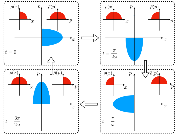
Figure 1: Sketch of the ( periodic) time evolution of the support of the Wigner function (in blue) for
the quench from a half-oscillator to an oscillator. Red: densities in () and in
().
Our goal in this paper is to study the time dependent Wigner function starting from this initial condition,
e.g. (3), (4),
and to understand how its bulk and edge properties evolve
with time, in particular whether their universality is
preserved under nonequilibrium dynamics.
We
obtain exact solutions for time dependent harmonic and inverse square potentials, and calculate the Wigner function and the density for various . For large , near the edges
where the density vanishes,
we obtain limiting kernels (of the Airy or Bessel types) that retain the form found
in the statics, up to a time dependent rescaling. It implies the occurrence of the
Tracy-Widom distribution [38]
for the position of the rightmost fermion [6].
For generic non-harmonic traps,
at large and intermediate times, the Wigner function is still uniform on the Fermi volume,
whose evolution can be more complex. We show that at generic points the
Fermi surf is still described by the same universal function as in
equilibrium (4), (33), with a space and time dependent
width that we calculate. We express multi-point and multi-time correlations
in terms of the Wigner function and its associated kernel. In the infinite time limit, we obtain exact
formula for the Wigner function under a thermalization hypothesis, which we show coincide
with the prediction of the Generalized Gibbs Ensemble (GGE) [39, 40].
The time evolved body wave function keeps the form of a Slater determinant
(6)
where the are the solutions of with initial condition , where , , are the single particles eigenstates of in increasing order
of energies .
We are interested in the quantum probability
,
described by the time dependent kernel
(7)
where the ’s form an orthonormal basis for all .
All -point correlations are determinants, ,
i.e. the ’s form a determinantal point process [41, 42].
One defines the -body Wigner function
Using the Schrödinger equation for the in (7) we
see that the kernel satisfies
(10)
which, via Fourier transformation, leads to the evolution equation
for , i.e. the Wigner equation (WE)
(11)
Although derived here for any , this equation does not explicitly depend on , hence
it is identical to the equation for [34]. It was also obtained
in second quantized form in [43, 31]. The crucial difference
thus lies in the initial condition, discussed above in the large limit, see
(3)-(4)-(5) at .
In the classical limit, i.e. setting in the WE, one obtains the Liouville equation (LE)
(12)
It verifies along the classical trajectories
and . Denoting , the
initial conditions (at ) as functions of the final ones (at ),
the general solution of the LE can thus be written as
where
is the initial Wigner function.
Let us start with the simplest solvable case of the harmonic oscillator, .
Since , the WE (11), reduces to the LE (12). Hence the solution is
(13)
which is a simple rotation in phase space of the initial Wigner function and is valid for any .
Let us specify the
initial Hamiltonian to be a harmonic oscillator, i.e.
in (2).
Hence the initial density is the semi-circle (1) for
large with .
Substituting the initial condition (3) into (13) one immediately
finds that for large the density remains a semicircle with
(14)
and . In fact a solution of the general time
dependent harmonic oscillator, ,
can be obtained for the same initial condition using the ‘rescaling’ method
[44, 45]. The wave functions are given by
(15)
where and
satisfies Ermakov’s equation
(16)
with , . The kernel and the density are
thus given in terms of their initial values, for any by
(17)
and .
In addition we obtain [46] the exact formula for
(18)
which reduces to (13) for .
Hence we see that for large the density remains a semi-circle
with an edge at , formula (14)
being recovered in the case . For the kernel,
the scaling forms obtained at equilibrium, namely the sine-kernel (in the bulk) and the
Airy kernel (at the edge) [8], are preserved, up to a
change in the scale. In particular the density at the
edge reads
(19)
with and a width
and .
The Wigner function method allows to study a variety of initial conditions.
One example is given by the harmonic oscillator restricted to
with an impenetrable wall at . The initial kernel, ,
is obtained
via the image method .
The associated Wigner function in the bulk is unity on the half-ellipse
with . Under evolution with , this
half ellipse rotates clockwise (see Fig. 1). Consider for
simplicity . Defining , ,
where ,
the density reads for
(20)
and in addition satisfies
and is time periodic of period .
Hence it is not a semi-circle, and there is now a moving front
(e.g. at for )
where the density vanishes linearly (see [46] for details).
A formula for can also be obtained for any and arbitrary initial condition (see [46]).
It is possible to extend the exact solution
to the case of an additional wall at , following [47]. Consider
(21)
and denote . The
initial kernel has an explicit expression [46] in terms of
Laguerre polynomials for any .
At large , the density in the bulk is a time-dependent half semi-circle
(22)
where is the same
solution of (16), e.g. for .
Near the wall the kernel takes the form
(23)
up to a phase factor, where
, , in terms of the Bessel kernel
(24)
characteristic of the ”hard-edge” universality class of RMT [22], thus
preserved by the dynamics in this case.
Consider now generic smooth confining potentials , , with .
Our strategy is as follows.
We first argue that, for large (or equivalently large ), obeys Liouville equation (12)
(and at is a theta function, i.e.
takes value in ). We then study the solution to the LE, leading to Burgers equation
and fermion hydrodynamics. Finally, we obtain the leading (quantum) corrections to that picture, of foremost
importance near the Fermi surf.
Let us expand (11) to the first ”quantum” order as
(25)
To check that the quantum terms are subdominant, we can
evaluate each term at using the initial condition (4)-(5). The derivatives
are non-zero only near the Fermi-surf: consider a generic point there, ,
such that , leading to . As increases,
we assume that and its derivatives still scale the same
way as , i.e. . Each order in brings acting on
and acting on , hence, using the scaling form (4)-(5),
a factor either or
. The latter dominates, but is
at large .
Under the Liouville equation the Fermi volume and surf are simply
transported by the (phase-space area preserving)
classical equation of motion, i.e.
(26)
There are several parametrizations to describe the
transported (and possibly wildly deformed) Fermi volume [46].
In the simplest case one can write
(27)
for the (single) support of the
number density .
For , each must then satisfy the Burgers equation
[48]
(28)
It recovers the standard free fermion hydrodynamics with a velocity field
with
, and
the local kinetic energy density
[46].
The equilibrium is recovered for with
(29)
and is time independent. The form (27) using (28)
automatically satisfies Liouville equation.
We now study the behavior of the Wigner function near the transported
Fermi-surf . We know that at it is given by (4)-(5)
and has a thickness . We thus look for a solution of (25) for of the form
(30)
with a time-dependent thickness , and .
Remarkably, plugging this form
into Eq.(25) allows to determine uniquely [46]
(31)
and , which is obeyed by . It also provides the correct matching with the initial condition,
since
on the Fermi surf. The solution corresponding to is obtained similarly
with . Furthermore
we show [46] that for smooth potentials, adding the missing higher order terms
in of the WE in Eq.(25) does not change the result.
Thus derivatives up to and including determine the
dynamical width, while only and enter the static width .
Hence we have found the universal scaling form near a generic
point of the transported Fermi-surf .
The width (31) can be calculated for any solving the Burgers equation (28)
with initial condition . Note that related
results were obtained
[49, 50, 51, 52] for a single particle in the
semi-classical limit, and for fermions at equilibrium
[35, 36]. Other expressions can be
obtained [46] at non-generic points, e.g. when
[51, 53, 37].
We assumed here that
the Fermi surf maintained its integrity, which in some cases
requires finite time. More generally, the section
of (such that iff )
can contain multiple intervals
which merge or disappear as varies. Locally, however,
as in the statics as long as one can find a smooth local parametrization
of the Fermi surf, similar scaling form as (30) should hold. This dynamical
scenario remains valid over a time scale when the Fermi surf does not change drastically from the initial
condition. Beyond this time scale, the dynamics
becomes quite different, as discussed later. However, it is hard to estimate precisely this time scale.
The above results can be extended to a quench from an initial system
prepared at finite temperature , in the grand canonical (GC)
ensemble with chemical potential . The equal time correlations
are again determinantal with the GC kernel (overbars denote GC averages)
(32)
with the mean occupation number of
the energy level of . The GC Wigner function
(defined in [37]) is again the Fourier transform of the GC kernel,
as in (9). It is clear from (32) that it obeys (10)
hence still the solution of (11), albeit with a different initial
condition. For large , in the bulk it reads
Introducing the important dimensionless parameter ,
the (same) Fermi surf is still well defined at low (with
) and Eq. (4) still applies with
(33)
a universal function depending only on
the dimensionless parameter (with in the limit).
Formula (13), (17), (18),
readily apply with, for large , these new initial conditions.
Eqs. (20), (24), (19)
admit extensions [46].
From the linearity of the W-equation (11) one can
express its solution at in terms of the solution as
(34)
since it holds at (equilibrium) as shown in [37].
At low near the Fermi surf, it allows to generalize Eq. (30)
(35)
where the dependence in of is indicated explicitly,
and the parameter acquires a dependence in , which
however disappears for the harmonic
oscillator for which ,
as for equilibrium.
We now study the multi-time quantum correlations.
As for equilibrium dynamics [25]
one shows from the Eynard-Mehta theorem [42] that
they are determinants based on the non-equilibrium space-time
extended kernel [54]
(36)
with for and for .
For instance the density-density correlation for reads
.
Consider now to be the -harmonic oscillator
and use the rescaling method. If is the
-harmonic oscillator, one easily obtains, up to a phase factor [46]
(37)
where obeys (16), and .
For , then as given in (14)
and .
Here is the equilibrium two time kernel of the
-harmonic oscillator studied in [25],
given by (36) with . This relation between and is
special to the harmonic oscillator.
is periodic in both times of
period , and of period .
Within a period decays very fast
in with a time scale in the bulk and at the edge
[25]. One can thus expand near and one obtains
the following scaling forms for . In the bulk
(38)
where is the real time continuation of the equilibrium extended sine kernel
given at e.g. in Eq. (70-71) of [25] and [46].
The width
and the velocity are new features of the
non-equilibrium dynamics ( at equilibrium). Near the edge
it takes the scaling form
(39)
where is the velocity of the edge and
is the equilibrium extended Airy kernel
(continued to real time)
given e.g. in Eq. (156) of [25] and [46].
Finally we discuss the large time behavior. In the ”classical” limit
, , it was shown recently [31] that
for generic confining potentials, e.g. different from the HO,
the Wigner function has a large time stationary limit. It was found
to coincide with the prediction of the GGE. Here we investigate this
question for fixed . Starting from the time-dependent kernel
(32), and expanding on the basis of the eigenfunctions
of (of energies )
we obtain
For a confining potential the spectrum of is non-degenerate,
hence the only non-oscillating terms are . Keeping only these
terms one obtains
(40)
where the are ”effective mean occupation numbers”,
with (i.e. at ),
as expected from particle number conservation. This is
the so-called diagonal approximation (DA) [39]
which, in the present case, can
also be obtained as a time average, i.e.
.
Under certain conditions, including absence of time periodicity, the large time limit exists
and then
. Let us define a fonction
such that
for all . Then one can obtain the diagonal Wigner function
(41)
in terms of the Wigner function, , associated to the ground state
of i.e to the kernel
(one first shows that and are related via (41), which implies
(41) for their Wigner functions). Note that if one defines
,
then ,
where is the density of states.
The above holds for arbitrary .
For large , we insert in
(41) the known form of the Wigner function
from (4), (5), (33), i.e.
and obtain one of our main result
(42)
where at , .
If one neglects the quantum width of the edge, for
fixed , it is equivalent to insert instead
in (41). This leads to
(43)
an approximation valid when
is much smaller than the width over which the
effective occupation number
drops from (for )
to (for ). This is the case in the
classical limit which we now consider
[55]. We note that is the probability density of the energy
of a single particle in the initial state. In the classical limit it is evaluated through
a phase space average over the initial Wigner function , which together with
(43) leads to
(44)
where is the semi-classical density of states.
This is our result in the classical limit . In the simplest
case considered in [31] (i.e. and a single orbit at each energy )
one has where
is the period of the classical orbit at energy . Inserting
, integrating over in
(44), and putting all together [46], one recovers
the large time limit result of [31] (obtained by a quite
different method)
valid in the classical case. Our formula (41)
is thus a good candidate for the large time limit of the Wigner function
in the quantum regime.
The GGE thermalization hypothesis [39, 40, 56] states that for local observables ,
,
where the density matrix involves an extensive
number of conserved quantities. For non-interacting fermions, as discussed in [39, 31],
these are the occupation numbers
of single particle energy levels of . The natural candidate is thus
where the are determined from the initial condition. One has
, where the are exactly the
ones obtained in (40) [46].
Hence one finds .
Thus we find that at the level of the single particle observables (the kernel and
Wigner function) the result of the GGE is identical to the diagonal
approximation.
What about the multi-point time dependent correlations ?
Since for any initial state equal to an eigenstate of , labeled by a set
of occupation numbers, , the time evolved state is determinantal,
correlations in this state have the form
Expanding on the eigenstates of now involves a sum over two sets of -fermion eigenstates
of .
The DA restricts that sum to identical eigenstates in both sets,
and one obtains [46] (after a grand canonical average)
(45)
where
.
This DA for differs from the prediction of the
simplest GGE ansatz discussed above. Indeed, the latter predicts
that the -point correlation is equal to the determinant
built from the kernel given in (40).
Agreement would hold only if
one could neglect the off-diagonal terms in the determinant
in (45), i.e. replace ,
as implied by the Cauchy-Binet identity. This occurs in some models, see a bosonic example in
[40] which has translational invariance and the GGE was shown to hold.
Here, connecting to the GGE (possibly in an inhomogeneous version
involving local Lagrange multipliers
) remains open.
In conclusion we studied the evolution of the Wigner function
for noninteracting fermions in after a quantum quench.
At times such that the integrity of the Fermi surf is retained, we found that
it is described by the same universal function as
at equilibrium, although with a space time dependent width that we calculated.
We obtained an exact candidate formula for the large time limit of the Wigner function
for generic (e.g. non-harmonic) confining potentials, and showed
that it agrees with the GGE. We calculated the diagonal approximation
to the many point correlations.
It would be interesting to
explore and detect these predictions in cold atom experiments.
Note added: at completion of this work we became aware
of the recent work in [57] which studies a related problem.
Acknowledgements.
We thank P. Calabrese for remarks and references, A. Borodin,
B. Doyon, A. de Luca and M. Fagotti for discussions,
and A. Krajenbrink for useful interactions at the initial stage of this work.
We acknowledge support from ANR grant ANR-17-CE30-0027-01 RaMaTraF.
References
[1]
S. Giorgini, L. P. Pitaevski, S. Stringari, Theory of ultra-cold Fermi gas,
Rev. Mod. Phys. 80, 1215 (2008).
[2]Y. Castin, Basic theory tools for degenerate Fermi gases in Ultra-cold Fermi Gases, ed. by
M. Inguscio, W. Ketterle, and C. Salomon, (2006), see also arXiv:0612613.
[3]
W. Kohn, A. E. Mattsson, Edge electron gas, Phys. Rev. Lett. 81 3487 (1998).
[4]
V. Eisler, Universality in the full counting statistics of trapped fermions, Phys. Rev. Lett. 111, 080402 (2013).
[5]
R. Marino, S. N. Majumdar, G. Schehr, P. Vivo, Phase transitions and edge scaling of number variance in Gaussian random matrices, Phys. Rev. Lett. 112, 254101 (2014).
[6]
D. S. Dean, P. Le Doussal, S. N. Majumdar, G. Schehr, Finite-temperature free fermions and the Kardar-Parisi-Zhang equation at finite time, Phys. Rev. Lett. 114, 110402 (2015).
[7]
D. S. Dean, P. Le Doussal, S. N. Majumdar, G. Schehr, Universal ground state properties of free fermions in a d-dimensional trap, Europhys. Lett. 112, 60001 (2015)
[8]
D. S. Dean, P. Le Doussal, S. N. Majumdar, G. Schehr, Non-interacting fermions at finite temperature in a d-dimensional trap: universal correlations, Phys. Rev. A 94, 063622 (2016).
[9]
N. Allegra, J. Dubail, J.-M. Stéphan, J. Viti, Inhomogeneous field theory inside the arctic circle, J. Stat. Mech. 053108 (2016).
[10]
J. Dubail, J. M. Stephan, J. Viti, P. Calabrese, Conformal field theory for inhomogeneous one-dimensional quantum systems: the example of non-interacting Fermi gases, SciPost Physics 2, 002 (2017).
[11]
I. Bloch, J. Dalibard, W. Zwerger, Many-body physics with ultracold gases, Rev. Mod. Phys. 80, 885 (2008).
[12]
L. W. Cheuk, M. A. Nichols, M. Okan, T. Gersdorf, R.Vinay, W. Bakr, T. Lompe, M. Zwierlein, Quantum-Gas Microscope for Fermionic Atoms, Phys. Rev. Lett. 114, 193001, (2015).
[13]
E. Haller, J. Hudson, A. Kelly, D. A. Cotta, B. Peaudecerf, G. D. Bruce, S. Kuhr, Single-atom imaging of fermions in a quantum-gas microscope, Nature Physics 11, 738 (2015).
[14]
M. F. Parsons, F. Huber, A. Mazurenko, C. S. Chiu, W. Setiawan, K. Wooley-Brown, S. Blatt, M. Greiner, Site-Resolved Imaging of Fermionic 6Li in an Optical Lattice, Phys. Rev. Lett. 114, 213002 (2015).
[15]
A. Omran, M. Boll, T. A. Hilker, K. Kleinlein, G. Salomon, I. Bloch, C. Gross, Microscopic observation of Pauli blocking in degenerate fermionic lattice gases, Phys. Rev. Lett. 115, 263001 (2015).
[16]
M. L. Mehta, Random Matrices, 2nd ed. (New York: Academic), (1991).
[17] P. J. Forrester,
Log-Gases and Random Matrices
(London Mathematical Society monographs, 2010).
[18]
P. J. Forrester, N. E. Frankel, T. M. Garoni, N. S. Witte, Painlevé transcendent evaluations of finite system density matrices for 1d impenetrable bosons, Commun. Math. Phys. 238, 257 (2003).
[19]
B. Lacroix-A-Chez-Toine, P. Le Doussal, S. N. Majumdar, G. Schehr, Statistics of fermions in a d-dimensional box near a hard wall, EPL 120,
10006 (2017).
[20]
F. D. Cunden, F. Mezzadri, N. O’ Connell, Free fermions and the classical compact groups, J. Stat. Phys. 171, 768 (2018).
[21]
K. Liechty, D. Wang, Asymptotics of free fermions in a quadratic well at finite temperature and the Moshe-Neuberger-Shapiro random matrix model, preprint arXiv:1706.06653.
[22]
B. Lacroix-A-Chez-Toine, P. Le Doussal, S. N. Majumdar, G. Schehr, Non-interacting fermions in hard-edge potentials, J. Stat. Mech. 123103 (2018).
[23]
A. Scardicchio, C. E. Zachary, S. Torquato, Statistical properties of determinantal point processes in high-dimensional Euclidean spaces, Phys. Rev. E 79, 041108 (2009).
[24]
J.-M. Stéphan, Free fermions at the edge of interacting systems, preprint arXiv:1901.02770.
[25]
P. Le Doussal, S. N. Majumdar, G. Schehr, Periodic Airy process and equilibrium dynamics of edge fermions in a trap
, Ann. Phys. 383, 312 (2017).
[26]
E. Quinn, M. Haque, Modulated trapping of interacting bosons in one dimension, Phys. Rev. A 90, 053609 (2014).
[27]
A. Minguzzi, D. M. Gangardt, Exact coherent states of a harmonically confined Tonks-Girardeau gas, Phys. Rev. Lett. 94, 240404 (2005).
[28]
M. Collura, M. Kormos, P. Calabrese, Quantum quench in a harmonically trapped one-dimensional Bose gas,
Phys. Rev. A 97, 033609 (2018).
[29]
M. Collura, S. Sotiriadis and P. Calabrese, Equilibration of a tonks-girardeau gas following a trap release,
Phys. Rev. Lett. 110, 245301 (2013), and Quench dynamics of a tonks-girardeau gas released
from a harmonic trap, Journal of Statistical Mechanics: Theory and Experiment 2013(09), P09025 (2013).
[30]
Y. Y. Atas, D. M. Gangardt, I. Bouchoule, K. V. Kheruntsyan, Exact nonequilibrium dynamics of finite-temperature Tonks-Girardeau gases, Phys. Rev. A 95, 043622 (2017).
[31]
M. Kulkarni, G. Mandal, T. Morita, Quantum quench and thermalization of one-dimensional Fermi gas via phase-space hydrodynamics, Phys. Rev. A 98, 043610 (2018).
[32]
E. Bettelheim, P. B. Wiegmann, Universal Fermi distribution of semiclassical nonequilibrium Fermi states, Phys. Rev. B 84, 085102 (2011).
[33]
E. Bettelheim, L. Glazman, Quantum ripples over a semiclassical shock, Phys. Rev. Lett. 109, 260602 (2012).
[34]
W. B. Case, Wigner functions and Weyl transforms for pedestrians, Am. J. Phys. 76, 937 (2008).
[35]
N. L. Balazs, G. G. Jr. Zipfel, Quantum oscillations in the semiclassical fermion -space density, Ann. Phys. 77, 139 (1973).
[36]
N. L. Balazs, G. G. Jr. Zipfel, The semiclassical fermion -space density in three dimensions, J. Math. Phys. 15, 2086 (1974).
[37]
D. S. Dean, P. Le Doussal, S. N. Majumdar, G. Schehr, Wigner function of noninteracting trapped fermions, Phys. Rev. A 97, 063614 (2018).
[38]
C. A. Tracy, H. Widom, Level-spacing distributions and the Airy kernel, Commun. Math. Phys. 159, 151 (1994).
[39]
For a review see F. H. Essler, M. Fagotti, Quench dynamics and relaxation in isolated integrable quantum spin chains, J. Stat. Mech. 064002 (2016).
[40]
S. Sotiriadis, P. Calabrese, Validity of the GGE for quantum quenches from interacting to noninteracting models, J. Stat. Mech. 07024 (2014).
[41]
See e.g. K. Johansson, Random matrices and determinantal processes, in Lecture Notes of the Les
Houches Summer School 2005 (A. Bovier, F. Dunlop, A. van Enter,
F. den Hollander, and J. Dalibard, eds.), Elsevier Science, (2006); arXiv:math-ph/0510038.
[42]
A. Borodin, Determinantal point processes, in The Oxford Handbook of Random Matrix Theory,
G. Akemann, J. Baik, P. Di Francesco (Eds.), Oxford University Press, Oxford (2011).
[43]
A. Dhar, G. Mandal, and S. R. Wadia, Classical Fermi fluid and geometric action for ,
Int. J. Mod. Phys. A 8, 325 (1993) and hep-th/9204028; A. Dhar, G. Mandal, and S. R. Wadia, Nonrelativistic fermions, coadjoint orbits of
and string field theory at , Mod. Phys. Lett. A 7, 3129 (1992) and [hep-th/9207011]; A. Dhar, G. Mandal, and S. R. Wadia, coherent states and path integral derivation of bosonization of nonrelativistic fermions in one-dimension, Mod. Phys. Lett. A 8, 3557 (1993) and [hep-th/9309028].
[44]
V. S. Popov, A. M. Perelomov, Parametric excitation of a quantum oscillator II, JETP 30, 910 (1969).
[45]
V. Gritsev, P. Barmettler, E. Demler, Scaling approach to quantum non-equilibrium dynamics of many-body systems, New J. Phys. 12, 113005 (2010).
[46]
D. S. Dean, P. Le Doussal, S. N. Majumdar, G. Schehr, Supplementary Material.
[47]
H. Kanasugi, H. Okada, Systematic treatment of general time-dependent harmonic oscillator in classical and quantum mechanics, Prog. Theor. Phys. 93, 949 (1995).
[48]
It is also the derivative of the eikonal equation for
the semi-classical action (with ),
see [46].
[49]
M. V. Berry, Semi-classical mechanics in phase space: a study of Wigner’s function, Phil. Trans. R. Soc. Lond. A 287, 237 (1977).
[50]
M. V. Berry, N. L. Balazs, Evolution of semiclassical quantum states in phase space, J. Phys. A: Math. Gen. 12, 625 (1979).
[51]
S. Filippas, G. N. Makrakis, Semiclassical Wigner function and geometrical optics,
Multiscale Model. Sim. , 674 (2003).
[52]
S. Filippas, G. N. Makrakis, On the evolution of the semi-classical Wigner function in higher dimensions, Eur. J. Appl. Math. 17, 33 (2006).
[53]
P. Le Doussal, S. N. Majumdar, G. Schehr, Multicritical edge statistics for the momenta of fermions in non-harmonic traps, Phys. Rev. Lett. 121, 030603 (2018).
[54]
Also equal to the expectation
(in second quantized notations).
[55]
At the relation between and is through
, leading to for a potential .
More generally with fixed corresponds to fixed ,
in which case .
[56]
C. Murthy, M. Srednicki, On relaxation to gaussian and generalized gibbs states in systems of particles with quadratic hamiltonians, arXiv:1809.03681.
[57]
P. Ruggiero, Y. Brun, J. Dubail,
Conformal field theory on top of a breathing one-dimensional gas of hard core bosons, preprint arXiv:1901.08132.