Optimal design strategy for non-Abelian geometric phases using Abelian gauge fields based on quantum metric

Abstract

Geometric phases, which are ubiquitous in quantum mechanics, are commonly more than only scalar quantities. Indeed, often they are matrix-valued objects that are connected with non-Abelian geometries. Here we show how generalized, non-Abelian geometric phases can be realized using electromagnetic waves travelling through coupled photonic waveguide structures. The waveguides implement an effective Hamiltonian possessing a degenerate dark subspace, in which an adiabatic evolution can occur. The associated quantum metric induces the notion of a geodesic that defines the optimal adiabatic evolution. We exemplify the non-Abelian evolution of an Abelian gauge field by a Wilson loop.

I Introduction

Geometry and quantum mechanics are inextricably linked. Whenever a quantum system evolves in Hilbert space, its wavefunction acquires a phase that solely depends on the path the quantum system has taken. This concept of geometric phases was introduced by Sir Michael Berry Berry who pointed out that there are instances in which these emerging phase factors cannot be removed by some gauge transformation. A famous example is the Aharonov–Bohm effect Aharonov in which the wavefunction of a charged particle travelling in a loop around a solenoidal magnetic field acquires a phase proportional to the flux through the surface enclosed by the loop, i.e. a line integral over the (Abelian) vector potential. Here the emerging (Abelian) phase is merely a complex number.

However, any quantum system with degenerate energy levels possesses a far richer structure as matrix-valued geometric phases Wilczek , known as non-Abelian holonomies. These can occur as soon as the emerging phase depends on the order of consecutive paths. In contrast to the vector potential in the Aharonov–Bohm scenario, a non-Abelian gauge field is responsible for the appearance of these matrix-valued phases. Such phases are crucial for topological quantum computation Zanardi ; Pachos , non-Abelian anyon statistics Nayak , and the quantum simulation of Yang–Mills theories. Non-Abelian synthetic gauge fields are usually realized in systems where coupled energy levels naturally lead to the required degeneracy such as in cold atomic samples Dalibard and artifical atoms in superconducting circuits Abdumalikov . In the case of electromagnetic fields, due to their intrinsic Abelian nature the required degeneracy is more intricate to design. One succesful scheme utilized the spin-orbit coupling of polarized light in asymmetric microcavities Ma .

In our work, we focus on a different degree of freedom and synthesize a non-Abelian geometric phase by implementing adiabatic population transfer Unanyan of light. We employ an integrated photonic structure possessing dark states, in which a non-Abelian geometric phase associated with a U(2) group transformation is realized. The quantum metric spanned by the subspace of the dark states induces a geodesic that defines the optimal adiabatic evolution of these non-Abelian phases.

II Theory

Gauge fields naturally arise in the context of field theories when demanding the invariance of a field under some transformation. Invariance under multiplication by a scalar phase factor leads to the concept of Abelian gauge fields, such as the four-vector potential of electromagnetism, with commuting components. In contrast, matrix-valued phases entail non-Abelian gauge fields where the commutator of the individual components involves the structure constants of the underlying Lie algebra. A famous example are Yang–Mills theories of particle physics Cheng .

A wavepacket evolving in the presence of a gauge field acquires a geometric phase. For Abelian gauge fields, this is the famous Berry–Pancharatnam phase Berry ; Pancharatnam . The non-Abelian generalization is known as the Wilson loop

$$W_{\mathcal{C}}=\mathrm{Tr}\left[\mathcal{P}\mathrm{exp}\left(-\oint_{\mathcal{C}}\mathbf{A}_{\nu}\mathrm{d}x^{\nu}\right)\right],$$ (1)

which is the trace of the path-ordered ($\mathcal{P}$) exponential of the non-Abelian gauge field $\mathbf{A}_{\nu}$ Wilson . Our system is a non-trivial collection of interacting Abelian subsystems and, thus, non-Abelian, being characterized by a Wilson loop $W_{\mathcal{C}}<2$ Goldman ; GoldmanSpielman .

In order to implement this concept, one seemingly requires a non-Abelian gauge field. However, this is not necessary, as a non-Abelian structure naturally appears whenever the evolution of a quantum system is confined to a degenerate subspace of some Hamiltonian Wilczek . As a consequence, generating non-Abelian geometric phases is not connected to the presence of a non-Abelian gauge fields, but to the existence of a degenerate subspace.

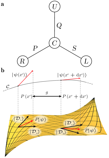
Figure 1: a Scheme of the four-waveguide system. b Visualization of changing dark subspace projector along curve $\mathcal{C}$. The change of the dark subspace projectors of the system is given by the quantum metric $g$.

In our work, we consider the system sketched in Fig. 1 that consists of four potential wells $C,U,R,L$ that are coupled with time-dependent hopping constants $Q,S,P$. The Schrödinger equation for the field amplitudes $a_{\textrm{\footnotesize{L}}},a_{\textrm{\footnotesize{U}}},a_{\textrm{\footnotesize{R}}},a_{\textrm{\footnotesize{C}}}$ in the individual wells reads, therefore,

$$\mathrm{i}\,\partial_{t}\left({\begin{array}[]{c}a_{\textrm{\footnotesize{L}}}\\ a_{\textrm{\footnotesize{R}}}\\ a_{\textrm{\footnotesize{U}}}\\ a_{\textrm{\footnotesize{C}}}\\ \end{array}}\right)=\left({\begin{array}[]{cccc}0&0&0&S\\ 0&0&0&P\\ 0&0&0&Q\\ S&P&Q&0\\ \end{array}}\right)\cdot\left({\begin{array}[]{c}a_{\textrm{\footnotesize{L}}}\\ a_{\textrm{\footnotesize{R}}}\\ a_{\textrm{\footnotesize{U}}}\\ a_{\textrm{\footnotesize{C}}}\\ \end{array}}\right)$$ (2)

This Hamiltonian supports two dark states with zero eigenvalue:

$$|\mathcal{D}_{1}\rangle =\sin\theta|w_{\textrm{\footnotesize{L}}}\rangle-\cos\theta|w_{\textrm{\footnotesize{R}}}\rangle,$$ (3)

$$|\mathcal{D}_{2}\rangle =\cos\theta\sin\phi|w_{\textrm{\footnotesize{L}}}\rangle+\sin\theta\sin\phi|w_{\textrm{\footnotesize{R}}}\rangle-\cos\phi|w_{\textrm{\footnotesize{U}}}\rangle,$$ (4)

where $|w_{\textrm{\footnotesize{U,R,L}}}\rangle$ are the eigenmodes of the potential wells $U,R,L$ respectively, with the angle parameterization $\theta=\arctan(P/S)$ and $\phi=\arctan(Q/\sqrt{S^{2}+P^{2}})$. Notably, they do not involve the eigenstate $|w_{\textrm{\footnotesize{C}}}\rangle$ to which all other states are coupled. These dark states span a (dark) subspace in which the adiabatic evolution of a wavefunction along a closed path can be described by a non-Abelian geometric phase (1) with the gauge field

$$(\mathbf{A}_{\nu})_{ki}=\langle\mathcal{D}_{k}|\frac{\partial}{\partial x^{\nu}}|\mathcal{D}_{i}\rangle,$$ (5)

written in the coordinates $\{x^{\nu}\}=\{S,P,Q\}$ (for details, see Supplementary Materials). In the context of adiabatic evolution, the Hamiltonian (2) is a generalization Unanyan of the STIRAP (STImulated Raman Adiabatic Passage) protocol STIRAP . What is required is to ensure adiabaticity of the evolution.

Interestingly, adiabatic transport is equivalent to parallel transport in a curved (metric) space via vanishing covariant derivative Liu , i.e. along a geodesic defined in our parameter manifold. The quantum metric $g_{\mu\nu}=\mathrm{Tr}\left(\partial_{\mu}P\partial_{\nu}P\right)$ is constructed from infinitesimal changes of the dark subspace projector $P(x^{\nu})=\sum_{i}|\mathcal{D}_{i}(x^{\nu})\rangle\langle\mathcal{D}_{i}(x^{\nu})|$ (see Fig. 1 B). This is the real part of a quantity known as the quantum geometric tensor Provost ; Rezakhani ; Nakahara ; Liu , whose imaginary part is the field strength tensor of the (non-Abelian) gauge field, $\mathbf{F}_{\mu\nu}=\partial_{\mu}\mathbf{A}_{\nu}-\partial_{\nu}\mathbf{A}_{\mu}-[\mathbf{A}_{\mu},\mathbf{A}_{\nu}]$.

The coordinates $x^{\nu}(z)$ in parameter space themselves are a function of the propagation distance $z$. The quantum metric $g_{\mu\nu}$ defines a path length (action) along the curve $\mathcal{C}$ in the parameter manifold from the input facet $z_{\textrm{\footnotesize{i}}}$ to the output facet $z_{\textrm{\footnotesize{f}}}$,

$$L=\int_{z_{\textrm{\footnotesize{i}}}}^{z_{\textrm{\footnotesize{f}}}}\sqrt{g_{\mu\nu}\partial_{z}x^{\mu}\partial_{z}x^{\nu}}\mathrm{d}z.$$ (6)

The principle of least action defines a geodesic that describes the evolution with the least diabatic error through parameter space Rezakhani . As a consequence, the notion of adiabaticity is intimately connected to the concept of the quantum metric. This defines the optimal strategy for determining the time dependence of the parameters for adiabatic evolution in parameter space. Starting from the desire to realize non-Abelian geometric phases, one first has to find a Hamiltonian with a degenerate subspace Wilczek on which a metric can be defined. The geodesic induced by this metric then specifies the variation of the parameters of the Hamiltonian such that the evolution through parameter space occurs with the least diabatic error. A closed path along the geodesic in parameter space then necessarily results in a non-Abelian geometric phase. In our experimental implementation, we minimize $L$ under the constraint of a given pulse shape, which provides the curves with the least diabatic error for a given total length $z_{\textrm{\footnotesize{f}}}-z_{\textrm{\footnotesize{i}}}$ (see Supplementary Materials).

III Experiment

In order to implement our findings, we employ a photonic platform manifested in the form of integrated coupled waveguides. Using the analogy between the quantum evolution of a wavefunction and the propagation of an optical wavepacket in the paraxial approximation Longhi , the quantum wells in our structure can be replaced by optical waveguides. The temporal evolution of the light amplitudes in those waveguides is governed by Eq. (2) with the sole difference that the time evolution is replaced by the evolution along the waveguides described by the spatial coordinate $z$ (see Fig. 2 A). Our design protocol yields a spatial evolution of the intersite hoppings $Q$, $S$, $P$ with an example depicted in Fig. 2 B. The hoppings $S$ and $P$ resemble the Stokes and pump pulses of Gaussian shape in the counterintuitive sequence known from STIRAP STIRAP , with $Q$ as an additional constant coupling. The evolution of the parameters in parameter space is chosen to form a closed-loop trajectory as shown in Fig. 2 C. Therefore, this evolution results in a geometric phase.

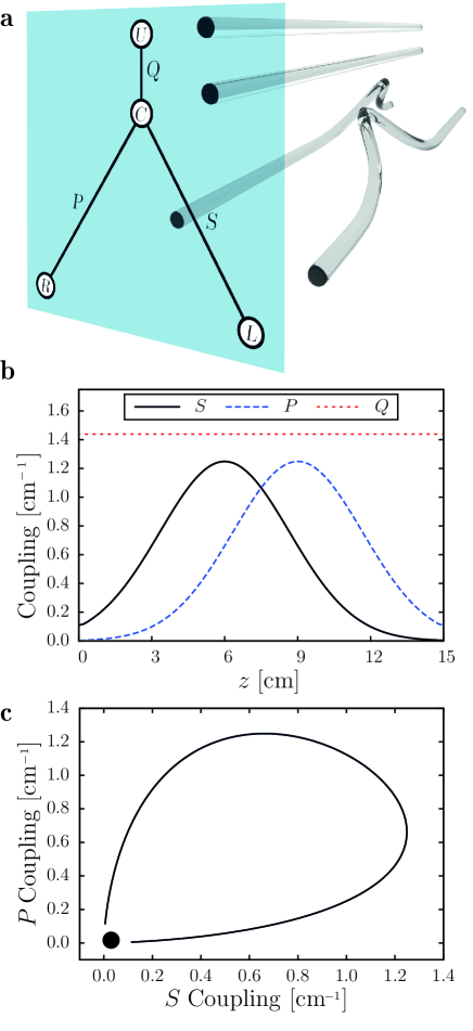
Figure 2: a 3D-rendering of the waveguides for one realization. b Coupling variation along propagating distance $z$. c Curve in the parameter manifold $\{S,P,Q\}$ ($Q=\textrm{const}$).

In the following, we will describe the measurement protocol for retrieving the Wilson loop. From the choice of the temporal evolution of the parameters $S$ and $P$, we have at the input facet $z_{\textrm{\footnotesize{i}}}$ and the output facet $z_{\textrm{\footnotesize{f}}}$ the relations $P(z_{\textrm{\footnotesize{i}}})/S(z_{\textrm{\footnotesize{i}}})\simeq 0\simeq S(z_{\textrm{\footnotesize{f}}})/P(z_{\textrm{\footnotesize{f}}})$. Hence, the dark states at both facets simply become $|\mathcal{D}_{1}(z_{\textrm{\footnotesize{i}}})\rangle=-|w_{\textrm{\footnotesize{R}}}\rangle$, $|\mathcal{D}_{2}(z_{\textrm{\footnotesize{i}}})\rangle=|w_{\textrm{\footnotesize{L}}}\rangle$ and $|\mathcal{D}_{1}(z_{\textrm{\footnotesize{f}}})\rangle=|w_{\textrm{\footnotesize{L}}}\rangle$, $|\mathcal{D}_{2}(z_{\textrm{\footnotesize{f}}})\rangle=|w_{\textrm{\footnotesize{R}}}\rangle$. As a consequence, launching light into the waveguides $L$ and $R$ excites only the dark states of the system. Also, measuring the light intensity emanating from the waveguides $L$ and $R$ at the output facet provides the information about the population transfer between the dark states. An initial superposition of the dark states evolves according to a unitary evolution $\mathbf{\mathcal{U}}$. As we show in the Supplementary Materials, the elements of this unitary matrix can be expressed in terms of the amplitudes of the dark states at the input and output facet. Moreover, the value of the Wilson loop is given by $W_{\mathcal{C}}=\mathrm{Tr}\left[\mathbf{\mathcal{U}}\right]$. Measuring the field intensities yields the absolute values of the matrix elements $|\mathcal{U}_{ki}|$, and hence the absolute value $|W_{\mathcal{C}}|$ as shown in the Supplementary Materials.

For the fabrication of our samples, we use the femtosecond laser writing technique Szameit . Details of the fabrication are given in the Methods section. We realize several structures with varying temporal profiles of the coupling parameters $S$ and $P$, resulting in different values of the Wilson loop. An example of the evolution along the waveguides recorded by fluorescence microscopy (see Methods) is shown in Fig. 3 A. Launching light into waveguide $L$ excites only the dark state $|\mathcal{D}_{2}(z_{\textrm{\footnotesize{i}}})\rangle$. During the evolution, the light is coupled to the waveguides $R$ and $U$ without ever populating $C$ (see Fig. 3 B). Hence, the evolution indeed remains in the dark subspace for all times as required for adiabaticity.

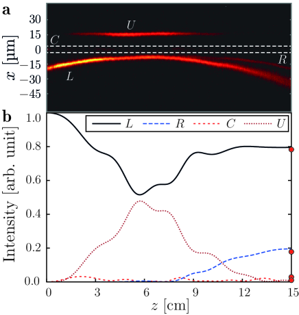
Figure 3: Intensity distribution in the four waveguides along the propagation distance. a Experimentally measured fluorescence signal which is proportional to the intensity in the waveguides. The waveguide L was excited, thus the second dark state. The central waveguide C is located between the dashed lines, highlighting the almost vanishing intensity. b Theoretically predicted intensity from the coupled-mode theory using Eq. (2). Red dots at the end facet are the experimentally measured intensities (compare Fig. 4).

For retrieving the elements of $\mathbf{\mathcal{U}}$, we measure the intensities at the output facet. A representative example is shown in Fig. 4 A. In our experiments, we realized Wilson loops by implementing three different sets of parameters (details of which are given in the Supplementary Materials). The results are summarized in Tab. 1, where the theoretical predictions and the experimental results are shown to agree well. In all three cases, the (absolute) value of the Wilson loop is well above $0$, thus proving the non-Abelian character of the underlying contour.

Table 1: Experimental results and corresponding theoretical Wilson loops for three different coupling variations. For detailed description of the used parameters and pulse shapes see the Supplementary Materials.

$|W_{\mathcal{C}}^{\textrm{\footnotesize{theo}}}|$	$|W_{\mathcal{C}}^{\textrm{\footnotesize{exp}}}|$
0.88	0.87
0.97	1.00
1.07	1.13

In order to prove that waveguide $C$ is part of the full eigenspace, we specifically launched light into $C$ and excited states in the bright subspace that extend over all waveguides (see Fig. 4 B). From our measurements, we find that at the output facet, all waveguides are bright such that one can conclude that, indeed, waveguide $C$ has to reside within the bright subspace.

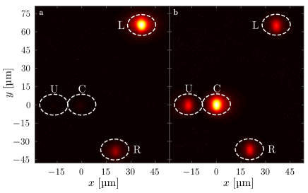
Figure 4: Measured intensities at the end facet. a Intensity distribution for dark-state excitation. This is for the same set of parameters as seen in Fig. 3. The result is clearly restricted to the dark subspace. b Intensity distribution for bright-state distribution. The waveguide C and U, and with that the bright states, are dominantly excited.

IV Conclusion

We employed evanescently coupled photonic waveguides to simulate the action of a non-Abelian gauge field on the dark subspace of the associated Hamiltonian. The non-Abelian nature of the process was verified by measurement of the gauge invariant Wilson loop. As the present implementation of the Wilson loop requires an adiabatic evolution within the dark subspace, the quantum metric is the appropriate tool to quantify the diabatic error.

Our results lay the foundations for the simulation of non-Abelian gauge fields using Abelian systems such as sound waves, matter waves or, in our case, light. In particular, within this construction principle, the implementation of non-Abelian gauge fields that transform under SU($N$) could be realized with $N+2$ coupled sites containing an $N$-dimensional dark subspace. Moreover, the use of geodesics of the quantum metric to quantify adiabaticity sheds new light on the optimization of all STIRAP-type processes.

The implementation of non-Abelian Abelian gauge fields prompts various important questions. One of them concerns the simulation of lattice gauge field theories such as Yang–Mills theories where Wilson loops are the observable quantities. In another context, using nonclassical light, our proposed setting is conducive to realize holonomic quantum operations as quantum logical gates can be defined as the action of non-Abelian geometric phases on the space of degenerate states, i.e. the dark subspace Pachos . Finally, the definition of a quantum metric induced by parametric changes of the waveguide couplings allows to study the evolution of a quantum system on curved manifolds.

V Acknowledgments

The authors acknowledge funding from the Deutsche Forschungsgemeinschaft (grants SCHE 612/6-1, SZ 276/20-1, SZ 276/15-1, BL 574/13-1, SZ 276/9-2) and the Krupp von Bohlen and Halbach foundation.

See pages 1 of SupplementalMaterials.pdf See pages 2 of SupplementalMaterials.pdf See pages 3 of SupplementalMaterials.pdf See pages 4 of SupplementalMaterials.pdf See pages 5 of SupplementalMaterials.pdf See pages 6 of SupplementalMaterials.pdf See pages 7 of SupplementalMaterials.pdf See pages 8 of SupplementalMaterials.pdf See pages 9 of SupplementalMaterials.pdf See pages 10 of SupplementalMaterials.pdf See pages 11 of SupplementalMaterials.pdf

References

- (1) M. V. Berry, Proc. Roy. Soc., Ser. A 392, 45 (1984).
- (2) Y. Aharonov and D. Bohm, Phys. Rev. 115, 485 (1959).
- (3) F. Wilczek and A. Zee, Phys. Rev. Lett. 52, 2111 (1984).
- (4) P. Zanardi and M. Rasetti, Phys. Lett. A 264, 94 (1999).
- (5) J. K. Pachos, Introduction to Topological Quantum Computation (Cambridge University Press, Cambridge, 2012).
- (6) C. Nayak, S.H. Simon, A. Stern, M. Freedman, and S. Das Sarma, Rev. Mod. Phys. 80, 1083 (2008).
- (7) J. Dalibard, F. Gerbier, G. Juzeliūnas, and P. Öhberg, Rev. Mod. Phys. 83, 1523 (2011).
- (8) A. A. Abdumalikov Jr., J. M. Fink, K. Juliusson, M. Pechal, S. Berger, A. Wallraff, and S. Filipp, Nature 496, 482 (2013).
- (9) L. B. Ma, S. L. Li, V. M. Fomin, M. Hentschel, J. B. Götte, Y. Yin, M. R. Jorgensen, and O. G. Schmidt, Nat. Commun. 7, 10983 (2016).
- (10) R. G. Unanyan, B. W. Shore, and K. Bergmann, Phys. Rev. A 59, 2910 (1999).
- (11) T.-P. Cheng and L.-F. Li, Gauge theory of elementary particle physics (Oxford University Press, Oxford, 1984).
- (12) S. Pancharatnam, Proc. Indian Acad. Sci. A. 44, 247 (1956).
- (13) K. G. Wilson, Phys. Rev. D 10, 2445 (1974).
- (14) K. Bergmann, H. Theuer, and B.W. Shore, Rev. Mod. Phys. 70, 1003 (1998).
- (15) J. P. Provost and G. Vallee, Commun. Math. Phys. 76, 289 (1980).
- (16) A. T. Rezakhani, D. F. Abasto, D. A. Lidar, and P. Zanardi, Phys. Rev. A 82, 012321 (2010).
- (17) S. Tanimura, M. Nakahara, and D. Hayashi, J. Math. Phys. 46, 022101 (2005).
- (18) Y.-Q. Ma, S. Chen, H. Fan, and W.-M. Liu, Phys. Rev. B 81, 245129 (2010).
- (19) S. Longhi, Laser & Photon. Rev. 3, 243 (2009).
- (20) A. Szameit and S. Nolte, J. Phys. B: At. Mol. Opt. Phys. 43, 163001 (2010).
- (21) N. Goldman, A. Kubasiak, P. Gaspard, and M. Lewenstein, Phys. Rev. A 79, 023624 (2009).
- (22) N. Goldman, G. Juzeliunas, P. Öhberg, and I. B. Spielman, Rep. Prog. Phys. 77, 126401 (2014).
- (23) J. Dell, J. L. deLyra, and L. Smolin, Phys. Rev. D 34, 3012 (1986).